A local constitutive model for the discrete element method. … · 2015-05-25 · A local...

Computational Particle Mechanics(will be inserted by the editor)

A local constitutive model for the discrete element method. Application togeomaterials and concrete

Eugenio Onate · Francisco Zarate · Juan Miquel · MiquelSantasusana · Miguel Angel Celigueta · Ferran Arrufat ·Raju Gandikota · Khaydar Valiullin · Lev Ring

Received: date / Accepted: date

Abstract This paper presents a local constitutive model for modelling the linear and non linear behavior ofsoft and hard cohesive materials with the discrete element method (DEM). We present the results obtained inthe analysis with the DEM of cylindrical samples of cement, concrete and shale rock materials under a uniaxialcompressive strength (UCS) test, different triaxial tests, a uniaxial strain compaction (USC) test and a braziliantensile strength (BTS) test. DEM results compare well with the experimental values in all cases.

Keywords Local constitutive model · Discrete element method · Geomaterials · Concrete

1 INTRODUCTION

Extensive research work on the discrete element method (DEM) has been carried out in the last decades sincethe first ideas were presented by Cundall and [11]. Much of the research efforts have focused on the developmentof adequate DEM models for accurately reproducing the correct behaviour of non cohesive and cohesive granularassemblies [1, 6, 8, 11, 20, 24, 29, 42, 45–47], as well as of solid materials [13, 14, 16–18, 22, 23, 28, 31, 32, 34–36, 42, 43]. In recent years the DEM has also been effectively applied to the study of multifracture and failure ofgeomaterials (soils and rocks), concrete, masonry and ceramic materials, among others.

The analysis of solids with the DEM poses a number of difficulties for adequate reproducing the correctconstitutive behaviour of the material under linear (elastic) and non linear conditions.

Within the analysis of solids with the DEM the material is typically represented as a collection of rigidparticles (spheres in three dimensions (3D) and discs in two dimensions (2D)) interacting among themselves atthe contact interfaces in the normal and tangential directions. Material deformation is assumed to be concentratedat the contact points. Appropriate contact laws are defined in order to obtain the desired macroscopic materialproperties. The contact law can be seen as the formulation of the material model of the underlying continuumat the microscopic level. For frictional cohesive material the contact law takes into account the cohesive bondsbetween rigid particles. Cohesive bonds can be broken, thus allowing to simulate fracture of the material and itspropagation.

E. Onate, F. Zarate, J. MiquelCentre Internacional de Metodes Numerics en Enginyeria (CIMNE)Campus Norte UPC, 08034 Barcelona, SpainUniversitat Politecnica de Catalunya (UPC)Tel.: +34-93-2057016Fax: +34-93-4016517E-mail: onate,zarate,[email protected]

M. Santasusana, M.A. Celigueta, F. ArrufatCentre Internacional de Metodes Numerics en Enginyeria (CIMNE)E-mail: msantasusana,maceli,[email protected]

R. GandikotaIndependent Consultant on Advanced Numerical Analysis E-mail: [email protected]

K. Valiullin, L. RingWeatherford InternationalE-mail: Khaydar.Valiullin,[email protected]

2 E. Onate, F. Zarate, J. Miquel, M. Santasusana, M.A. Celigueta, F. Arrufat, R. Gandikota, K. Valiullin, L. Ring

Fig. 1: Model of the contact interface in the DEM

A challenge in the failure analysis of solid materials, such as cement, shale rock and concrete, with the DEMis the definition of the limit strengths in the normal and shear directions at the contact interfaces, and thecharacterization of the non linear relationship between forces and displacements at these interfaces beyond theonset of fracture, accounting for frictional effects, damage and plasticity.

In this work we present a local constitutive model for failure analysis of solid materials typical in geomechanicsand concrete applications with the DEM. The model is validated in the analysis of cement, concrete and shalerock samples for several laboratory strength tests. The tests considered include the uniaxial compression strength(UCS) test, triaxial compressive strength tests, the uniaxial strain compaction (USC) test and the brazilian tensilestrength (BTS) test. DEM results compare well with experimental data provided by Weatherford for the cementand shale rock samples [19, 33] and the Technical University of Catalonia (UPC) for the concrete samples [37].

2 CONSTITUTIVE MODELS FOR THE DEM

Standard constitutive models in the DEM are typically characterized by the following parameters:

Local parameters– Normal and shear stiffness parameters Kn and Ks.– Normal and shear strength parameters Fn and Fs.– Coulomb friction coefficient µ.– Local damping coefficient Cn.

Global parameters– Global damping coefficient for the translational motion, αt.– Global damping coefficient for the rotational motion, αn.

Figure 1 shows an scheme of some DEM parameters for a 2D model.The challenge in DEM models for analysis of solids is finding an objective and accurate relationship between

the DEM parameters and the standard constitutive parameters of a continuum mechanics model (hereafter called“continuum parameters”): the Young modulus E, the Poisson ratio ν and the tension and shear failure stresses

σft and τf , respectively.Two different approaches can be followed for determining the DEM constitutive parameters for a cohesive

material, namely the global approach and the local approach. In the global approach uniform global DEM propertiesare assumed for each contact interface in the whole discrete element assembly. The values of the global DEMparameters can be found via different procedures. Some authors haver derived analytical relationships betweencontinuum and global DEM parameters [24, 25]. Others have used numerical experiments for determining therelationships between DEM and continuum parameters expressed in dimensionless form [14, 17, 18]. This methodhas been used by the authors in previous works [21–23, 31, 34–36]. Other procedures are based on relating theglobal DEM and continuum parameters via laboratory tests using inverse analysis techniques [29].

The local approach used in this work assumes that the DEM parameters depend on the local properties ofthe interacting particles, namely their radii and the continuum parameters at each interaction point. Differentalternatives for defining the DEM parameters via a “local approach” have been reported in recent years [13, 14,16, 31, 32, 42, 43]. A comparative study of several global and local approaches for estimating the DEM constitutiveparameters is presented in [36].

In this work we present a new procedure for defining the DEM parameters for a cohesive material in theframework of the local approach. In the next section we describe how the local elastic parameters can be found.Then we define appropriate local failure criteria at the contact interface using an elasto-damage model for the

A local constitutive model for the discrete element method. Application to geomaterials and concrete 3

Fig. 2: Motion of a rigid particle

normal tensile stress and the shear stress, and an elasto-plastic model for the normal compressive stress. Theaccuracy of the local DEM constitutive model is verified in the analysis of laboratory strength tests for differentcohesive materials.

The DEM model presented here can be considered as an extension of that proposed by Donze and co-workers[13, 16, 38, 43]. Among the distinct features of our model we note the inclusion of the effect of the size ofthe interacting spheres in the normal and shear parameters, the introduction of a parameter in the constitutivelaw accounting for the number of contacts and the packaging of particles, the definition of the failure criteria,the estimation of the limit compressive stress at the contact interface, the effect of damage and plasticity in theevolution of the normal and shear parameters and the definition of the material parameters in terms of the uniaxialstress-strain curve obtained from strength tests.

Clearly, the local DEM constitutive model presented in this work is also applicable to standard non-cohesivegranular material, as a particular case of the more general expressions for the cohesive case. In this sense, the modelis able to simulate the frictional behaviour of the particulate material that forms once the bonds are broken.

3 BASIC EQUATIONS

3.1 Equations of motion

The translational and rotational motion of rigid spherical or cylindrical particles is described by means of thestandard equations of rigid body dynamics. For the i-th particle we have (Figure 2)

miui = Fi , (1)

Iiωi = Ti , (2)

where ui is the particle centroid displacement in a fixed (inertial) coordinate frame X, ωi – the angular velocity,m – the particle mass, Ii – the moment of inertia, Fi – the resultant force, and Ti – the resultant moment aboutthe central axes. Vectors Fi and Ti are sums of: (i) all forces and moments applied to the i-th particle due toexternal loads, Fexti and Text

i , respectively, (ii) contact interactions with neighbouring particles Fij (Figure 3),j = 1, · · · , nci , where nci is the number of particles being in contact with the i-th particle, (iii) forces and moments


Fig. 3: Force Fij at the contact interface between particles i and j

resulting from external damping, Fdampi and Tdampi , respectively. Thus, we can be write as

Fi = Fexti +

nci∑

j=1

Fij + Fdampi (3)

Ti = Texti +

nci∑

j=1

rijc Fij + Tdampi (4)

where rcij is the vector connecting the centroid of the i-th particle with the contact point c at the interface betweenparticles i and j (Figure 3).

The form of the rotational equation (2) holds for spheres and cylinders (in 2D) and is simplified with respectto a general form for an arbitrary rigid body with the rotational inertial properties represented by a second ordertensor. In the general case it is more convenient to describe the rotational motion with respect to a co-rotationalframe x which is embedded at each element, since in this frame the tensor of inertia is constant.

3.2 Integration of the equations of motion

Equations (1) and (2) are integrated in time using a standard central difference scheme [31, 48]. The time integrationoperator for the translational motion at the n-th time step is as follows:

uni =Fnimi

, (5)

un+1/2i = u

n−1/2i + uni ∆t (6)

un+1i = uni +∆ui with ∆ui = u

n+1/2i ∆t (7)

The first two steps in the integration scheme for the rotational motion are identical to those given by Eqs.(5) and(6):

ωni =Tni

Ii, (8)

ωn+1/2i = ω

n−1/2i + ωni ∆t (9)

The vector of incremental rotation ∆θ = [∆θx, ∆θy, ∆θz]T is calculated for the ith particle as

∆θi = ωn+1/2i ∆t (10)

Knowledge of the incremental rotation suffices to update the tangential contact forces. It is also possible to trackthe rotational position of particles, if necessary. Then the rotation matrices between the moving frames embedded


in the particles and the fixed global frame must be updated incrementally using an adequate multiplicative scheme[23, 31, 48].

Explicit integration in time yields high computational efficiency and it enables the solution of large models.The disadvantage of the explicit integration scheme is its conditional numerical stability imposing the limitationon the time step ∆t [48], i.e.

∆t ≤ ∆tcr (11)

where ∆tcr is a critical time step determined by the highest natural frequency of the system ωmax as

∆tcr =2

ωmax(12)

If damping exists, the critical time increment is given by

∆tcr =2

ωmax

(√1 + ξ2 − ξ

)(13)

where ξ is the fraction of the critical damping corresponding to the highest frequency ωmax. Exact calculationof the highest frequency ωmax requires the solution of the eigenvalue problem defined for the whole system ofconnected rigid particles. In an approximate solution procedure, an eigenvalue problem can be defined separatelyfor every rigid particle using the linearized equations of motion

miai + kiai = 0 (14)

wheremi = {mi,mi,mi, Ii, Ii, Ii}T , ai = {(ux)i, (uy)i, (uz)i, (θx)i , (θy)i , (θz)i}T (15)

and ki is the stiffness matrix accounting for the contributions from all the interface constraints that are active forthe i-th particle.

4 FRICTIONAL CONTACT CONDITIONS

4.1 Contact interface

Let us assume that an individual particle is connected to the adjacent ones by appropriate relationships at thecontact interfaces. These relationships define either a perfectly bond or a frictional sliding situation at the interface.

Particles are assumed to be spherical and can have very different sizes. Each particle i is characterized by thesphere radius ri. We will assume that particles i and j are in contact at a point c located at a distance (1 + β)rior (1 + β)rj from the centers of particles i and j, respectively (Figure 4) where β is a positive number (typically)0 ≤ β ≤ 0.20. We define the interaction domain between the two particles that share the contact point c as acylinder of radius equal to the radius of the smaller of the two particles in contact. The circular section at point cof radius rc is the contact interface between particles i and j.

This definition of the contact interface and the interaction domain is motivated by the fact that the twointeracting particles can have very different radius for an arbitrary distribution of the particle sizes. The contactinterface is thus limited by the size of the smaller of the two particles in contact.

4.2 Interaction range

The overall behaviour of a material can be reproduced by associating a simple constitutive law to each contactinterface. The interaction between spherical (in 3D) or circular (2D) particles i and j with radius ri and rj ,respectively is defined within an interaction range. This range allows for a certain gap or an overlapping betweenthe particles. Then two particles will interact if

1− β ≤ dijri + rj

≤ 1 + β (16)

where dij is the distance between the centroids of particles i and j and β is the interaction range parameter (Figures3 and 4). This choice is made so that the DEM can simulate materials other than simple granular materials, in


Fig. 4: Definition of contact interface. (a) β 6= 0. (b) β = 0

particular those which involve a matrix, as it is found for instance in concrete, cement and rock. A value of β > 0is chosen in order to model the effect of this matrix that may glue two aggregates which are not themselves incontact. In this manner the model can handle the presence of gaps and overlappings generated by most of thesphere meshers. Simply, the contact search is extended using a value of β > 0 and the equilibrium position of thecontact point is then set for its initial configuration (which is not always a tangential contact of particles). Thisworks inwards for particle inclusions or outwards for gaps. For the problems solved in this work we have takenβ = 0.10.

From Eq.(16) we deduce

dij = (1± β)(ri + rj) (17)

where the plus and minus sign accounts for the gap and overlapping between the two particles, respectively.

4.3 Contact search algorithm

Changing contact pairs of elements during the analysis are automatically detected. The simple approach to identifyinteraction pairs by checking every particle against every other one would be very inefficient, as the computationaltime is proportional to n2, where n is the number of elements. In our formulation the search is performed usinga grid-based algorithm. In this case the computation time of the contact search is proportional to n lnn, whichallows us to solve large frictional contact systems involving many particles [23].

4.4 Decomposition of the contact force

Once contact between a pair of particles has been detected, the forces occurring at the contact point are calculated.The interaction between the two interacting particles can be represented by the contact forces Fij and Fji, whichsatisfy the following relation:

Fij = −Fji (18a)


Fig. 5: Decomposition of the contact force into its normal and tangential components

Fig. 6: Forces and stresses acting on a contact interface section Aij . Definition of normal and shear directions

We decompose Fij into its normal and shear components, Fijn and Fijs , respectively (Figure 5)

Fij = Fijn + Fijs = Fnnij + Fijs (18b)

where nij is the unit vector normal to the contact interface between particles i and j and Fn is the modulus ofthe normal force at the interface. Eq.(18b) implies that the normal force lies along the line connecting the centersof the two particles in contact and directed outwards from particle i (Figure 5).

The shear force Fijs along the shear direction (Figure 6) can be written as

Fijs = Fs1s1 + Fs2s2 (19a)

where Fs1 and Fs2 are the shear force components along the shear directions s1 and s2, and s1 and s2 are unitvectors in these directions. Vector s1 is taken in an arbitrary direction orthogonal to the normal vector. Thens2 = nij × s1.

The shear force modulus Fs is obtained as

F ijs = |Fijs | = (F 2s1 + F 2

s2)1/2 (19b)

The relationship between the contact forces Fn, Fs1 and Fs2 and the particle displacements are obtained usingthe local constitutive model described in the next section.

4.5 Definition of the contact law

In this work we have assumed a proportionality between the normal force at each contact interfaces and therelative displacement and the relative velocity of the contact point. As for the shear force, this has been assumedto be proportional to the relative sliding motion at the contact point. The proportionality coefficients have been


estimated starting from the one-dimensional stress-strain relationship for the cylindrical contact domain of Figure4. This approach has been preferred versus the contact laws proposed by Hertz [15] and Mindlin [27] for modellingthe contact interaction between two spheres in the normal and tangential directions, respectively. These laws havebeen used to model the contact force in granular material with the DEM [4, 46]. For the solids material consideredin this work, the existence of a matrix between grains (modelled via a gap distance, Eq.(16)) prevents in mostcases the direct contact between particles, which justifies the more “diffusive” contact model chosen in this work.

A comparison of different contact has shown that simple models in the DEM contact models such as thatpresented here lead to equivalent and, sometimes even better, results than more sophisticated models [12].

5 LOCAL DEFINITION OF DEM ELASTIC CONSTITUTIVE PARAMETERS

5.1 Normal force parameters

The normal force Fn at the contact interface between particles i and j is obtained as

F ijn = σnAij (20)

where σn is the normal stress at the contact interface and Aij is the effective area at the interface computed as

Aij = αijAij with Aij = πr2c (21)

Recall that rc is the radius of the smaller of the two particles interacting at the interface ij (Figure 4).In Eq.(21) αij is a parameter that accounts for the fact that the number of contacts and the packaging of

particles are not optimal. Clearly, αij is a local parameter for the ij interface. In this work, however, we haveconsidered the case of spherical particles only and used a global definition of αij as

αij = α = 40P

Nc(22)

where Nc and P are the average number of contacts per sphere and the average porosity for the whole particleassembly. Eq.(22) has been deduced by defining the optimal values for the number of contacts per sphere and forthe global porosity equal to 10 and 25%, respectively. Clearly α ' 1 for quasi-optimal packaging distributions, asit is the case for the particle meshes using in the examples solved in this work.

The normal stress σn is related to the normal strain between the interacting spheres, εn, by a visco-elastic lawas

σn = Eεn + cεn (23)

where E is the Young modulus of the solid material.We note that the Young modulus is assumed to be an intrinsic property of the material. As such it is typically

characterized from axial tests on cylindrical samples. Thus, the Young modulus obtained from the experimentalaxial stress-strain relationship is used for defining the local normal stress-strain relationship at a macroscopic level(23) at the contact interfaces. The same applies to the definition of the Poisson’s ratio of the material used fordefining the local shear constitutive relationship in Section 5.2.

The normal strain and the normal strain rate are defined as

εn =undij

, εn =undij

(24)

where dij is given by Eq.(17).Substituting Eq.(24) into (23) gives

σn =1

dij[Eun + cun] (25)

In Eqs.(24) and (25), c is a local damping coefficient per unit length and un and un are the normal (relative)displacement and the normal (relative) velocity at the contact point defined as

un = (xj − xi) · nij − dij , un = (uj − ui) · nij (26)

where xi and xj are the position vectors of the centroids of particles i and j. Note that un and un express therelative (incremental) motion between the centroids of the interacting particles.


The damping coefficient c is taken as a fraction ξ of the critical damping c per unit length for the system oftwo rigid spherical bodies with masses mi and mj connected by a spring of stiffness Kn [23, 31], i.e.

c =ξc

rc= 2

ξ

rc

√mijKn (27)

with 0 < ξ ≤ 1 and mij is the reduced mass of the contact,

mij =mimj

mi +mj(28)

In our work we have taken ξ = 0.9.From Eqs.(20) and (25) we deduce the relationship between the normal force and normal relative motion at

the interface between particles i and j as

F ijn =Aij

dij(Eun + cun) = Knun + Cnun (29)

Substituting Eqs.(21) and (27) into (29) we find the expression of the normal stiffness and normal viscous(damping) coefficients at the contact interface as

Kn =αijπr

2c

dijE Cn =

2πrcαijξ

dij

√mijKn (30)

Eq.(29) is assumed to hold in the elastic regime for both the normal tensile force Fnt and the normal compressiveforce Fnc

.

5.2 Shear force parameters

A similar approach is followed for obtaining the relationship between the shear forces and the relative tangentialdisplacements at each contact interface.

The shear forces in the s1 and s2 directions (Figure 6) are given by

Fs1 = τ1Aij , Fs2 = τ2A

ij (31)

where τ1 and τ2 are the shear stresses at the contact interface. These stresses are linearly related to the shearstrains γ1 and γ2 at the interface by

τ1 = Gγ1 , τ2 = Gγ2 (32)

where G is the shear modulus.A simple definition of the shear strains is

γ1 =us1dij

, γ2 =us2dij

(33)

where us1 and us2 are the components in the s1 and s2 directions of the relative tangential displacement vectorat the contact point given by (Figure 6)

uijs = [us1 , us2 ]T = uij − (uij · nij)nij (34a)

withuij =

(∆ui + (ωωωωωωωωωωωωωωi × rci)∆t

)−(∆uj + (ωωωωωωωωωωωωωωj × rcj )∆t

)(34b)

where ∆ui and ∆uj are the displacement increments of the centroids of particles i and j, respectively (Eq.(7))and rci and rcj are the vectors connecting the particle centers with the contact point (Figure 5).

Substituting Eqs.(32) and (33) into (31) we find

Fs1 = Ks1us1 and Fs2 = Ks2us2 (35)

with

Ks1 = Ks2 = Ks =Kn

2(1 + ν)(36)


where ν is the Poisson ratio.From Eqs.(35) we can obtain a relationship between the modulus of the shear force and the modulus of the

shear displacement vector asFs = Ksus (37)

withFs = |Fijs | =

[(Fs1)2 + (Fs2)2

]1/2, us = |uijs | =

[(us1)2 + (us2)2

]1/2(38)

The sign of Fsk (k = 1, 2) in Eqs.(35) depends on the sign of the velocity component usk , while in Eq.(37) onlythe modulus of vectors Fijs and uijs are involved.

For convenience the upper indices i, j are omitted hereonwards in the expression of the normal and shear forcevectors Fijn and Fijs at a contact interface.

6 GLOBAL BACKGROUND DAMPING FORCE

A quasi-static state of equilibrium for the assembly of particles can be achieved by application of an adequateglobal damping to all particles. This damping adds to the local one introduced at the contact interface (Section5.1). We have considered the following non-viscous type global damping terms

Fdampi = −αt|Fext

i + Fij | ui|ui|

(39)

Tdampi = −αr|Ti|

ωi|ωi|

(40)

The definition of the translational and rotational damping parameters αt and αr is a topic of research. Apractical alternative is to define αt and αr as a fraction of the stiffness parameters Kn and Ks, respectively. Inour work we have taken αt = αr = 0.1. Alternative a viscous type damping can be used, as described in [23, 31].

7 ELASTO-DAMAGE MODEL FOR TENSION AND SHEAR FORCES

7.1 Normal and shear failure

In this model, cohesive bonds at a contact interface are assumed to start breaking when the interface strength isexceeded in the normal direction by the tensile contact force, or in the tangential direction by the shear force. Theuncoupled failure (decohesion) criterion for the normal and tangential directions at the contact interface betweenparticles i and j is written as

Fnt ≥ Fnt , Fs ≥ Fs (41)

where Fntand Fs are the interface strengths for pure tension and shear-compression conditions, respectively, Fnt

is the normal tensile force and Fs is the modulus of the shear force vector defined in Eq.(38).The interface strengths are defined as

Fnt= σft A

ij , Fs = τf Aij + µ1|Fnc| (42)

where σft and τf are the tensile and shear failure stresses, respectively (also called tensile and shear strengths), Fnc

is the compressive normal force at the contact interface and µ1 = tanφ1 is a (static) friction parameter, where φ1 isan internal friction angle. These values are assumed to be an intrinsic property of the material and are determinedexperimentally. In our work σft is taken as the tensile strength of the material measured in a bending-tensile (BT)

test (i.e. σft = (σft )BT ). The value of σft can also be obtained from the failure stresses in a Brazilian TensileStrength (BTS) test using the relationship between the tensile strength in BTS and BT tests. For the examples

presented in this paper we have accepted that σtf = (σft )BT = 1.60(σft )BTS [2, 5].

In absence of values from specific tensile strength tests the tensile strength σft can also be estimated from themaximum compressive stress, (σfnc

)UCS, in a uniaxial compressive strength (UCS) test in a cylindrical sample. Atypical relationship for concrete, used in this work, is

σft = 0.464[(σfnc

)UCS]2/3

(43)


There is a big discrepancy in the literature for the value of the shear strength τf for frictional cohesive materials.In our work we have estimated the value of τf as a percentage of the maximum compressive stress in an UCS test,(σfnc

)UCS , as

τf = β(σfnc)UCS (44)

where β is a parameter that is calibrated in numerical experiments via UCS and BTS tests. In our numericalexperiments for cement, concrete and shale rock materials the value of β used has ranged from 0.4 < β < 0.55.The corresponding value of τf is in agreement with the experimental results of Talbot [41] and Anderson et al.[3] for estimating the shear strength of cement and concrete materials more than are century ago, as well as withmore recent experimental data for concrete and rocks [9, 10, 39, 40, 44].

Following tension failure, the constitutive behavior in the shear direction is governed by the standard Coulomblaw

Fs = µ2|Fnc| us|us|

with µ2 = tanφ2 (45)

where µ2 is a dynamic Coulomb friction coefficient and φ2 is the post-failure internal friction angle. Both µ2 andφ2 are determined from experimental tests.

Figure 7a shows the graphical representation of the failure criterium described by Eqs.(41), (42) and (45). Thiscriterium assumes that the tension and shear forces contribute to the failure of the contact interface in a decoupledmanner. On the other hand, shear failure under normal compressive forces follows a failure line that is a functionof the shear failure stress, the compression force and the internal friction angle.

Indeed, a coupled failure model in the tension-shear zone can also be used, as shown in Figure 7b. For thenumerical tests presented in the paper the uncoupled model has been used.

Figure 8 shows the evolution of the normal tension force Fntand the shear force Fs at a contact interface until

failure in terms of the relative normal and tangential displacements. The effect of damage in the two constitutivelaws is also shown in the figure. The method for introducing damage in the constitutive equations is explained inthe next section.

Fig. 7: Failure line in terms of normal and shear forces. (a) uncoupled failure model. (b) Coupled failure model

7.2 Damage evolution law

Elastic damage under tensile and shear conditions has been taken into account in this work by assuming a linearsoftening behaviour defined by the softening moduli Hn and Ht introduced into the force-displacement relationshipsin the normal (tensile) and shear directions, respectively (Figure 8).


Fig. 8: Undamaged and damaged elastic moduli under tension (a) and shear (b) forces

The constitutive relationships for the elasto-damage model are written as

Normal (tensile) direction

For 0 < dn ≤ 1 : Fnt = (1− dn)Knulnunun = Kd

nun with Kdn = (1− dn)

ulnunKn

For dn ≥ 1 : Fnt = 0

Shear direction

For 0 < ds ≤ 1 : Fs = (1− ds)Ksulsusus = Kd

sus with Kds = (1− ds)

ulsusKs

For ds > 1 : Fs = µ2|Fnc|

(46)

where dn and ds are scalar damage parameters in the normal (tensile) and shear directions at the contact interface,respectively and Kd

n and Kds are damaged elastic stiffness parameters. The damage parameters dn and ds are a

measure of the loss of mechanical strength at each contact interface. For the undamaged state dn = 0 and ds = 0,while for a damaged state 0 < dn ≤ 1 and 0 < ds ≤ 1.

Damage effects are assumed to start when the strength failure conditions (41) are satisfied. The evolution ofthe damage parameters from the value zero to one can be defined in a number of ways using fracture mechanicsarguments. A key issue is that the area under the line defining the force (relative) displacement relationship in thedamaged region (the shadowed area in Figure 8) equals the specific fracture energy of the material [26, 30, 31].

The following damage parameters are defined for convenience

δn =ufn − ulnuln

, δs =ufs − ulsuls

(47)

where ufn and ufs are values of the interface displacement increments in the normal and shear directions at failurecomputed as

ufn = dijεfn , ufs =

√Aijγfs (48)

where εfn and γfs are respectively the failure normal strain and the failure shear strain. These strains are an intrinsicproperty of the material that has to be obtained experimentally.

In our work we have defined dn and ds using a simple linear strain softening law as

dn =

0 for un < uln =

Fnt

Kn1

δn

(unuln− 1

)for uln ≤ un < ufn

1 for un ≥ ufn

(49a)

ds =

0 for us < uls =

FsKs

1

δs

(usuls− 1

)for uls ≤ us < ufs

1 for us ≥ ufs

(49b)


The failure conditions evolve due to damage as follows

Fnt≥ Fdnt

, Fs ≥ Fds (50)

with Fdnt= Fnt

−Hn

(un − uln

)Fds = Fs −Ht

(us − uls

) (51)

where (Fnt,Fdnt

) and (Fs,Fds ) are the undamaged and damage interface strengths for pure tension and pure shearconditions, respectively.

Figure 9 shows the evolution of the failure lines from the undamaged to the fully damaged state for theuncoupled model of Figure 7a.

Fig. 9: Evolution of the failure lines due to damage for uncoupled normal and shear failure

8 ELASTO-PLASTIC MODEL FOR COMPRESSION FORCES

The compressive stress-strain behaviour in the normal direction at the contact interface for frictional cohesivematerials, such as cement, rock and concrete, is typically governed by an initial elastic law followed by a non-linearconstitutive equation that varies for each material. The compressive normal stress increases under linear elasticconditions until it reaches the limit normal compressive stress σlnc

(also called yield stress). This is defined as theaxial stress level where the experimental curve relating the axial stress and the axial strain starts to deviate fromthe linear elastic behaviour. After this point the material is assumed to yield under elastic-plastic conditions.

The elasto-plastic relationships in the normal compressive direction are defined as

Loading path

dFnc= KTn

dun (52a)

Unloading pathdFnc

= Kn0dun (52b)

In Eqs.(52) dFnc and dun are respectively the increment of the normal compressive force and the normal(relative) displacement, Kn0

is the initial (elastic) compressive stiffness for a value of E = E0 (Figure 10), andKTn

is the tangent compressive stiffness given by

KTn=ETE0

Kn0(53)

where ET is the slope of the normal stress-strain curve in the elastoplastic branch (i.e. KT = E1, E2, E3 in Figure10).

Plasticity effects in the normal compressive direction also affect the evolution of the tangential forces at theinterface, as the interface shear strength is related to the normal compression force by Eq.(42).


Figure 10 shows the diagram relating the compressive axial stress and the compressive axial strain used formodelling the elasto-plastic constitutive behaviour at the contact interfaces. The form of each diagram is typicallyobtained from experimental tests on cylindrical samples with the adjustment explained in the next section.

The diagram in Figure 10 will be used for modelling with the DEM the tests in cement, concrete and shalerock material in this work.

LCS1 = σlnc: limit compressive stress defining the onset of elastoplastic behaviour at the contact interface

Fig. 10: Compressive axial stress-compressive axial strain diagram for elastoplastic material

9 LIMIT COMPRESSIVE STRESS AT THE CONTACT INTERFACE. EXPERIMENTALADJUSTMENT

The limit compressive stress at the contact interface is obtained by correcting the experimental value of the limitcompressive stress obtained in a UCS test. The correction is needed for taking into account the micro-macrorelationship that relates the limit normal stress at the contact interfaces with the limit compressive stress obtainedfrom experimental tests.

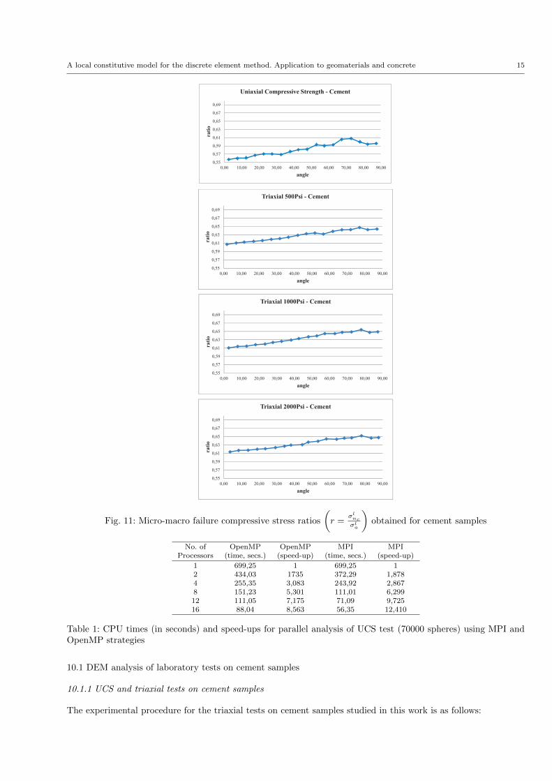
Figure 11 shows the average values of the ratio r =σlnc

σla

at all the contact interfaces in terms of the angle that

the normal vector to the interface forms with the horizontal axis for different triaxial tests on cement samples.In the expression of r, σlnc

is the limit normal compressive stress at the contact interface and σla is the limitcompressive stress obtained in a UCS test. The results displayed in Figures 14 show that the values of r rangeform 0.55–0.65 for UCS and triaxial tests.

The conclusion of this study is that the limit normal compressive stress at the contact interface, σlnc, is a

proportion of the actual limit compressive stress in a experimental test. In our work we have computed σlncas

σlnc= 0.6.(σlnc

)UCS , where (σlnc)UCS is the yield stress obtained in a UCS test.

10 NUMERICAL EXPERIMENTS

The DEM model presented in the previous sections has been implemented in the DEMPACK code (www.cimne.com/dempack), based on routines from the open-source object-oriented software platform KRATOS (www.cimne.com/kratos) and the pre-postprocessing system GiD (www.gidhome.com). DEMPACK is a fully parallelized DEM code.Table 1 shows the computer times and speed-ups for the analysis of a UCS test with a DEM mesh of 70000 spheresand 1000 time steps using different processors in a Intel Xeon ES-2670 machine (2×8 = cores) using OpenMP andMPI parallel computing strategies. Typically, the MPI strategy provided a better speed up in all cases. Note thatthe problem was solved in some 56 seconds using 16 processors. Indeed, this speed can be improved by enhancingthe parallel computing features of the code.


0,55

0,57

0,59

0,61

0,63

0,65

0,67

0,69

0,00 10,00 20,00 30,00 40,00 50,00 60,00 70,00 80,00 90,00

rati

o

angle

Uniaxial Compressive Strength - Cement

0,55

0,57

0,59

0,61

0,63

0,65

0,67

0,69

0,00 10,00 20,00 30,00 40,00 50,00 60,00 70,00 80,00 90,00

rati

o

angle

Triaxial 500Psi - Cement

0,55

0,57

0,59

0,61

0,63

0,65

0,67

0,69

0,00 10,00 20,00 30,00 40,00 50,00 60,00 70,00 80,00 90,00

rati

o

angle


0,55

0,57

0,59

0,61

0,63

0,65

0,67

0,69

0,00 10,00 20,00 30,00 40,00 50,00 60,00 70,00 80,00 90,00

rati

o

angle


Fig. 11: Micro-macro failure compressive stress ratios

(r =

σlnc

σla

)obtained for cement samples

No. of OpenMP OpenMP MPI MPIProcessors (time, secs.) (speed-up) (time, secs.) (speed-up)

1 699,25 1 699,25 12 434,03 1735 372,29 1,8784 255,35 3,083 243,92 2,8678 151,23 5,301 111,01 6,29912 111,05 7,175 71,09 9,72516 88,04 8,563 56,35 12,410

Table 1: CPU times (in seconds) and speed-ups for parallel analysis of UCS test (70000 spheres) using MPI andOpenMP strategies

10.1 DEM analysis of laboratory tests on cement samples

10.1.1 UCS and triaxial tests on cement samples

The experimental procedure for the triaxial tests on cement samples studied in this work is as follows:


Fig. 12: Uniaxial strain compaction test in cement sample [19]. Normal total compressive stress-axial strain rela-tionship

1. A right cylindrical plug is cut from the sample core and its ends ground parallel each other within 0.001 inch.Physical dimensions and weight of the specimen are recorded. The dimensions of the cylindrical samples are 1inch diameter and 2 inches height. The specimen is tested under saturated condition with water.

2. The specimen is then placed between two endcaps and a heat-shrink jacket is placed over the specimen.3. Axial strain and radial strain devices are mounted in the endcaps and on the lateral surface of the specimen,

respectively.4. The specimen assembly is placed into the pressure vessel and the pressure vessel is filled with hydraulic oil.5. Confining pressure is increased to the desired hydrostatic testing pressure.6. Specimen assembly is brought into the contact with a loading piston that allows application of axial load.7. Increase axial load at a constant rate until the specimen fails or axial strain reaches a desired amount of strain

while confining pressure is held constant.8. Reduce axial stress to the initial hydrostatic condition after sample fails or reaches a desired axial strain.9. Reduce confining pressure to zero and disassemble sample.

The simulation of a triaxial test with the DEM reproduces the experiment as follows.

a) The confining pressure is applied up to the desired hydrostatic testing pressure.b) A prescribed axial motion is applied at the top of the specimen until this fail, or the axial compressive strain

strain reaches a desired amount of strain while confining pressure is held constant.

For the UCS test the process starts by step (b) above described with zero confinement pressure.We note that the goal of this study was to reproduce with the DEM model presented the structural behaviour

of the sample during the axial compression phase. For this purpose an average Young modulus (deduced from theuniaxial strain compaction (USC) test) was chosen for modelling the the hydrostatic compaction of the sampleduring the application of the confining pressure. A more detailed study of the non linear behaviour of the cementsample under an hydrostatic load will be presented in a subsequent work.

Figure 12 shows the normal stress-strain relationship for a cement material as deduced from the USC testpresented in [19]. The curve shows an initial elastic branch and a (elasto-plastic) hardening branch.

Figure 13 shows the so-called “differential stress” computed as the difference between the applied axial stressand the confinement pressure during the USC test for the same cement material [19]. The curve shows the initiallinear elastic part, a limit axial stress of around 10 Mpa and the subsequent non linear branch. The non linearregion has a flat part which indicates the compaction of the cement material for that stress level. This is followedby a hardening branch which evidences the recovery of the material stiffness for high compaction values.

For completeness, Figure 14 shows the evolution of confinement pressure during the USC test. We note thatthe curve in Figure 13 is the difference between the curves of Figures 12 and 14.

The stress in the curve in Figure 13 coincides with the effective stress only if we accept that the water pressurein the pores is the same as the external pressure required to enforce the uniaxial strain conditions during the test.

In our work we have used the stress-strain curve obtained in the USC test as the basis for computing thenormal compressive force at the contact interfaces (σa) for the cement material examples. Note that for saturatedconditions this curve already accounts for the effect of water pressure at the pores.


Fig. 13: Uniaxial strain compaction test in cement sample [19]. Differential stress between the applied axial stressand the confinement pressure

Fig. 14: Uniaxial strain compaction test in cement sample [19]. Confinement pressure versus axial deformation

ρ µ1 µ2 E0 ν σft τf(g/cc) (GPa) (MPa) (MPa)

1.70 0.30 0.40 3.80 0.20 4.80 8.50

Table 2: Material parameters for cement

LCS1 LCS2 LCS3 YRC1 YRC2 YRC3 δn δs α(MPa) (MPa) (MPa)

8.5 9.0 11 3 9 24 0.20 0.2 1.0

Table 3: DEM constitutive parameters for the UCS, USC and BTS tests on cement samples

Tables 2–4 show the material and DEM parameters for the cement material studied in this work. Table 2 showsthe basic material parameters reported in [19]. The tensile strength σft has been deduced from the BTS test value

of (σft )BTS = 2.92 MPa [19] using the relationship σft = 1.60(σft )BTS ' 4.80 MPa as mentioned in Section 7.1. Onthe other hand, τf has been taken as τf = 1

2 (σfnc)UCS = 8.50 MPa, where (σfnc

)UCS is the maximum compressivestress obtained in the UCS test.


Confining LCS1 LCS2 LCS3 YRC1 YRC2 YRC3 δn δs αpressure (Psi) (MPa) (MPa) (MPa)

500 9.5 11 13 3 9 24 0.20 0.2 1.01000 10 11 14 3 9 24 0.20 0.2 1.02000 13 14 15 3 9 24 0.20 0.2 1.04000 21 23 26 3 9 24 0.20 0.2 1.0

Table 4: DEM constitutive parameters for triaxial tests on cement samples

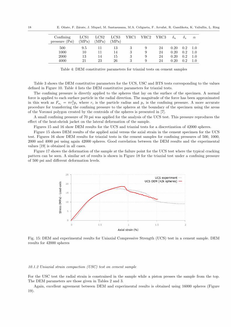
Table 3 shows the DEM constitutive parameters for the UCS, USC and BTS tests corresponding to the valuesdefined in Figure 10. Table 4 lists the DEM constitutive parameters for triaxial tests.

The confining pressure is directly applied to the spheres that lay on the surface of the specimen. A normalforce is applied to each surface particle in the radial direction. The magnitude of the force has been approximatedin this work as Fni

= πr2i pc where ri is the particle radius and pc is the confining pressure. A more accurateprocedure for transferring the confining pressure to the spheres at the boundary of the specimen using the areasof the Voronoi polygon created by the centroids of the spheres is presented in [7].

A small confining pressure of 70 psi was applied for the analysis of the UCS test. This pressure reproduces theeffect of the heat-shrink jacket on the lateral deformation of the sample.

Figures 15 and 16 show DEM results for the UCS and triaxial tests for a discretization of 42000 spheres.

Figure 15 shows DEM results of the applied axial versus the axial strain in the cement specimen for the UCStest. Figures 16 show DEM results for triaxial tests in the cement samples for confining pressures of 500, 1000,2000 and 4000 psi using again 42000 spheres. Good correlation between the DEM results and the experimentalvalues [19] is obtained in all cases.

Figure 17 shows the deformation of the sample at the failure point for the UCS test where the typical crackingpattern can be seen. A similar set of results is shown in Figure 18 for the triaxial test under a confining pressureof 500 psi and different deformation levels.

Fig. 15: DEM and experimental results for Uniaxial Compressive Strength (UCS) test in a cement sample. DEMresults for 42000 spheres

10.1.2 Uniaxial strain compaction (USC) test on cement sample

For the USC test the radial strain is constrained in the sample while a piston presses the sample from the top.The DEM parameters are those given in Tables 2 and 3.

Again, excellent agreement between DEM and experimental results is obtained using 16000 spheres (Figure19).


(a) Confining pressure = 500psi

(b) Confining pressure = 1000psi

Fig. 16: Triaxial tests in cement samples. DEM-Drill and experimental results for confining pressures of a) 500psi,b) 1000psi. DEM results for 42000 spheres

10.1.3 Brasilian tensile strength (BTS) test on cement sample

The BTS test was carried out for a sample of 1.487in diameter and 0.863in thickness. The density of the materialwas 1.70g/cm3. The experimental value of the maximum load in the BTS test was 847 lb which corresponds to a

value of (σft )BTS = 420 psi ≈2.9 MPa. Hence, σft = 1.6(σft )BTS = 4.8 Mpa (Section 7.1).

The DEM parameters used are given in Tables 2 and 3.

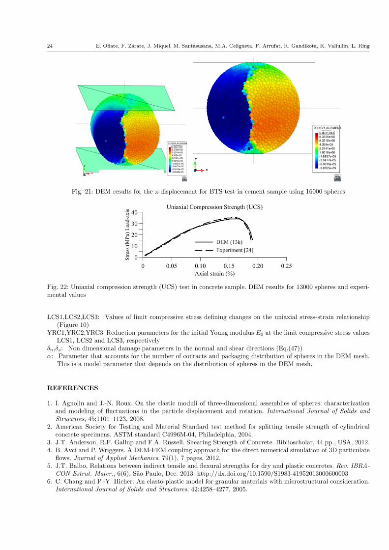
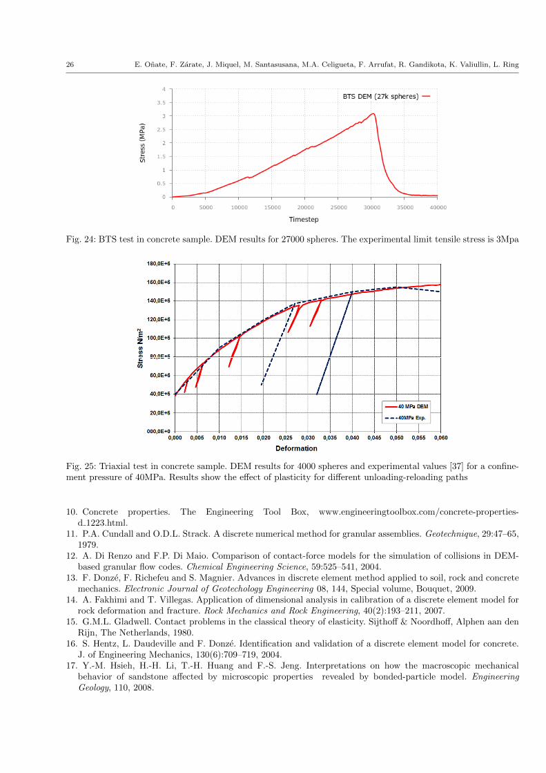
The DEM analysis was carried out using a discretization of 16000 spheres. The stress-displacement curveobtained with the DEM is displayed in Figure 20. The maximum tensile strength computed is 3.0 MPa. Theagreement with the experimental value of 2.9MPa is within 3.5% of relative error.

Figure 21 shows the x-displacement field on the sample once it has broken.

10.2 DEM analysis of laboratory tests on concrete samples

The experimental tests were carried out at the laboratories of the Technical University of Catalonia (UPC) inBarcelona, Spain. Details of the test are given in [37]. The concrete used in the experimental study was designed tohave a characteristic compressive strength of between 32.8 and 38 MPa at 28 days. Standard cylindrical specimens(of 150 mm diameter and 300 mm height) were cast in metal molds and demolded after 24 hours for storage in afog room.

The triaxial tests were prepared with a 3-mm-thick butyl sleeve placed around the cylinder and an impermeableneoprene sleeve fitted over it. Before placing the sleeves, two pairs of strain gages were glued on the surface of the


(c) Confining pressure = 2000psi

(d) Confining pressure = 4000psi

Fig. 16: (Cont.) Triaxial tests in cement samples. DEM and experimental results for confining pressures of c)2000psi and d) 4000psi. DEM results for 42000 spheres

specimen at mid-height. Steel loading platens were placed at the flat ends of the specimen and the sleeves weretightened over them with metal scraps to avoid the ingress of oil.

The tests were performed using a servo-hydraulic testing machine with a compressive load capacity of 4.5 MNand a pressure capacity of 140 MPa. The axial load from the testing machine is transmitted to the specimen bya piston that passes through the top of the cell. Several levels of confining pressure ranging from 1.5 MPa to 60MPa were used in order to study the brittle-ductile transition of the response. First the prescribed hydrostaticpressure was applied in the cell, and then the axial compressive load was increased at a constant displacementrate of 0.0006 mm/s.

Two specimens were tested at each confining pressure, and all tests were performed at ages of more than 50days to minimize the effect of aging response. In addition to the triaxial tests, uniaxial compression tests were alsoperformed.

Concrete samples were tested in dry conditions. For our computations the limit compressive normal stress wasestimated as the stress level of the axial stress-deformation curve where elasto-plastic behaviour initiates in theUCS test [37] (Figure 22) and taking into account the correction mentioned in Section 9. This gives σlnc

= 15 Mpa.

On the other hand, the value of σft was estimated using Eq.(43) for a value of (σfnc)UCS = 37 MPa. This gives

σft ' 5 MPa. As for τf we have taken τf = 0.45(σfnf)UCS ' 16 MPa.

The DEM constitutive parameters for the analysis of the concrete samples are shown in Table 5. Figures 22and 23 respectively show DEM results for the UCS and triaxial tests for confining pressures of 4.5, 9.0 and 60MPa using a discretization of 13000 spheres. Results for the BTS test are shown in Figure 24. Good agreementwith the experimental results [37] was found in all cases.


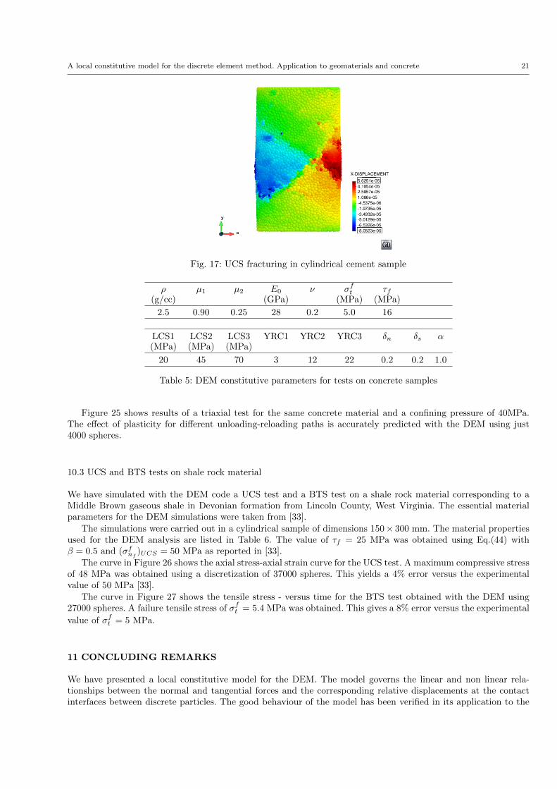
Fig. 17: UCS fracturing in cylindrical cement sample


2.5 0.90 0.25 28 0.2 5.0 16


20 45 70 3 12 22 0.2 0.2 1.0

Table 5: DEM constitutive parameters for tests on concrete samples

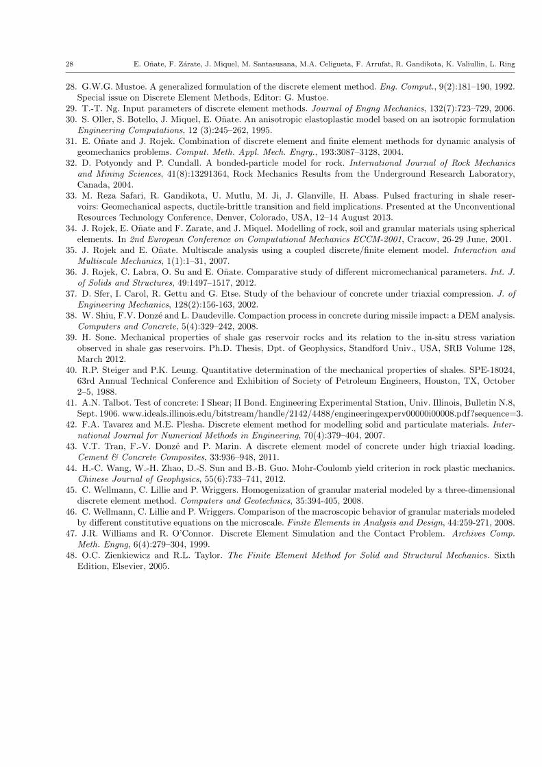
Figure 25 shows results of a triaxial test for the same concrete material and a confining pressure of 40MPa.The effect of plasticity for different unloading-reloading paths is accurately predicted with the DEM using just4000 spheres.

10.3 UCS and BTS tests on shale rock material

We have simulated with the DEM code a UCS test and a BTS test on a shale rock material corresponding to aMiddle Brown gaseous shale in Devonian formation from Lincoln County, West Virginia. The essential materialparameters for the DEM simulations were taken from [33].

The simulations were carried out in a cylindrical sample of dimensions 150× 300 mm. The material propertiesused for the DEM analysis are listed in Table 6. The value of τf = 25 MPa was obtained using Eq.(44) withβ = 0.5 and (σfnf

)UCS = 50 MPa as reported in [33].

The curve in Figure 26 shows the axial stress-axial strain curve for the UCS test. A maximum compressive stressof 48 MPa was obtained using a discretization of 37000 spheres. This yields a 4% error versus the experimentalvalue of 50 MPa [33].

The curve in Figure 27 shows the tensile stress - versus time for the BTS test obtained with the DEM using27000 spheres. A failure tensile stress of σft = 5.4 MPa was obtained. This gives a 8% error versus the experimental

value of σft = 5 MPa.

11 CONCLUDING REMARKS

We have presented a local constitutive model for the DEM. The model governs the linear and non linear rela-tionships between the normal and tangential forces and the corresponding relative displacements at the contactinterfaces between discrete particles. The good behaviour of the model has been verified in its application to the


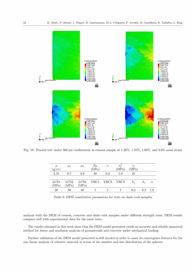
Fig. 18: Triaxial test under 500 psi confinement in cement sample at 1.28%, 1.55%, 1.80%, and 2.0% axial strain


2.55 0.7 0.6 30 0.2 5.0 25


20 30 40 1 1 1 0.2 0.2 1.0

Table 6: DEM constitutive parameters for tests on shale rock samples

analysis with the DEM of cement, concrete and shale rock samples under different strength tests. DEM resultscompare well with experimental data for the same tests.

The results obtained in this work show that the DEM model presented yields an accurate and reliable numericalmethod for linear and nonlinear analysis of geomaterials and concrete under mechanical loading.

Further validation of the DEM model presented is still needed in order to asses its convergence features for thenon linear analysis of cohesive material in terms of the number and size distribution of the spheres.


Fig. 19: DEM results for Uniaxial Strain Compaction (USC) test on cement sample using 16000 spheres

Fig. 20: DEM results for Brasilian Strength (BTS) test in cement sample using 16000 spheres

12 ACKNOWLEDGEMENTS

This work was carried out with financial support from Weatherford, the Advanced Grant Projects SAFECON andCOMDESMAT of the European Research Council and the BALAMED project (BIA2012-39172) of MINECO,Spain.

The support of CIMNE for making available the codes DEMPACK (www.cimne.com/dempack) and KRATOS(www.cimne.com/kratos) and GiD (www.gidhome.com) is gratefully acknowledged.

ANNEX

We list below the key analysis parameters involved in the DEM model presented. All the parameters, except α aremacroscopic material parameters that should be determined from experimental tests.

ρ: Densityµ1: Static (Coulomb) friction coefficientµ2: Dynamic (Coulomb) friction coefficientE0: Young modulus at the onset of the uniaxial compression testsν: Poisson’s ratioσft : Tensile failure stressτf : Shear failure stress


Fig. 21: DEM results for the x-displacement for BTS test in cement sample using 16000 spheres

Fig. 22: Uniaxial compression strength (UCS) test in concrete sample. DEM results for 13000 spheres and experi-mental values

LCS1,LCS2,LCS3: Values of limit compressive stress defining changes on the uniaxial stress-strain relationship(Figure 10)

YRC1,YRC2,YRC3 Reduction parameters for the initial Young modulus E0 at the limit compressive stress valuesLCS1, LCS2 and LCS3, respectively

δn,δs: Non dimensional damage parameters in the normal and shear directions (Eq.(47))α: Parameter that accounts for the number of contacts and packaging distribution of spheres in the DEM mesh.

This is a model parameter that depends on the distribution of spheres in the DEM mesh.

REFERENCES

1. I. Agnolin and J.-N. Roux, On the elastic moduli of three-dimensional assemblies of spheres: characterizationand modeling of fluctuations in the particle displacement and rotation. International Journal of Solids andStructures, 45:1101–1123, 2008.

2. American Society for Testing and Material Standard test method for splitting tensile strength of cylindricalconcrete specimens. ASTM standard C4996M-04, Philadelphia, 2004.

3. J.T. Anderson, R.F. Gallup and F.A. Russell. Shearing Strength of Concrete. Biblioscholar, 44 pp., USA, 2012.4. B. Avci and P. Wriggers. A DEM-FEM coupling approach for the direct numerical simulation of 3D particulate

flows. Journal of Applied Mechanics, 79(1), 7 pages, 2012.5. J.T. Balbo, Relations between indirect tensile and flexural strengths for dry and plastic concretes. Rev. IBRA-

CON Estrut. Mater., 6(6), Sao Paulo, Dec. 2013. http://dx.doi.org/10.1590/S1983-419520130006000036. C. Chang and P.-Y. Hicher. An elasto-plastic model for granular materials with microstructural consideration.

International Journal of Solids and Structures, 42:4258–4277, 2005.


(a) Triaxial Load - 4.5MPa Pressure

(b) Triaxial Load - 9.0MPa Pressure

(c) Triaxial Load - 60MPa Pressure

Fig. 23: Triaxial tests in concrete samples. DEM results for 13000 spheres and experimental values for confinementpressures of (a) 4.5MPa, (b) 9.0MPa, (c) 60 MPa

7. G. Cheung and C. O’Sullivan. Effective simulation of flexible lateral boundaries in two- and three dimensionalDEM simulations. Particuology, 6:483–500, 2008.

8. P.W. Cleary. Industrial particle flow modelling using DEM. Engineering Computations, 29:698–793, 2009.9. J.M. Cook, M.C. Sheppard and O.H. Houwen. Effects of strain rate and confining pressure on the deformation

and failure of shale. SPE Drilling Engineering, pp. 100–104, June 1991.


Fig. 24: BTS test in concrete sample. DEM results for 27000 spheres. The experimental limit tensile stress is 3Mpa

Fig. 25: Triaxial test in concrete sample. DEM results for 4000 spheres and experimental values [37] for a confine-ment pressure of 40MPa. Results show the effect of plasticity for different unloading-reloading paths

10. Concrete properties. The Engineering Tool Box, www.engineeringtoolbox.com/concrete-properties-d 1223.html.

11. P.A. Cundall and O.D.L. Strack. A discrete numerical method for granular assemblies. Geotechnique, 29:47–65,1979.

12. A. Di Renzo and F.P. Di Maio. Comparison of contact-force models for the simulation of collisions in DEM-based granular flow codes. Chemical Engineering Science, 59:525–541, 2004.

13. F. Donze, F. Richefeu and S. Magnier. Advances in discrete element method applied to soil, rock and concretemechanics. Electronic Journal of Geotechology Engineering 08, 144, Special volume, Bouquet, 2009.

14. A. Fakhimi and T. Villegas. Application of dimensional analysis in calibration of a discrete element model forrock deformation and fracture. Rock Mechanics and Rock Engineering, 40(2):193–211, 2007.

15. G.M.L. Gladwell. Contact problems in the classical theory of elasticity. Sijthoff & Noordhoff, Alphen aan denRijn, The Netherlands, 1980.

16. S. Hentz, L. Daudeville and F. Donze. Identification and validation of a discrete element model for concrete.J. of Engineering Mechanics, 130(6):709–719, 2004.

17. Y.-M. Hsieh, H.-H. Li, T.-H. Huang and F.-S. Jeng. Interpretations on how the macroscopic mechanicalbehavior of sandstone affected by microscopic properties revealed by bonded-particle model. EngineeringGeology, 110, 2008.


Fig. 26: Axial stress-axial strain curve for UCS test in shale rock material. DEM results using 37000 spheres

Fig. 27: Tensile stress-time curve for BTS test in shale rock material. DEM results using 27000 spheres

18. H. Huang. Discrete element modeling of tool-rock interaction. Ph.D. Thesis, December, University of Min-nesota, 1999.

19. O. Kwon. Rock mechanics testing & analyses. Cement mechanical testing. Weatherford Laboratories Report,WFT Labs RH-45733, March 2010.

20. N. Kruyt, and L. Rothenburg. Kinematic and static assumptions for homogenization in micromechanics ofgranular materials. Mechanics of Materials, 36(12):1157–1173, 2004.

21. C. Labra and E. Onate. High-density sphere packing for discrete element method simulations. Communicationsin Numerical Methods in Engineering, 25(7):837–849, 2009.

22. C. Labra, J. Rojek, E. Onate and F. Zarate. Advances in discrete element modelling of underground excavations. Acta Geotechnica, 3(4):317–322, 2009.

23. C. Labra. Advances in the development of the discrete element method for excavation processes. Ph.D. Thesis.Technical University of Catalonia, UPC, July 2012.

24. C.-L. Liao, T.-C. Chan, D.-H. Young and C.S. Chang. Stress-strain relationship for granular material basedon the hypothesis of best fit. Int. J. Solids and Structures, 34(31-32):4087–4100, 1995.

25. C.-L. Liao and T.-C. Chan. A generalized constitutive relation for a randomly packed particle assembly.Computers and Geomechanics, 20(3-4):345–363, 1997.

26. J. Lubliner, S. Oller, J. Oliver and E. Onate. A plastic damage model for concrete. Int. Journal of Solids andStructures, 25(3):299–326, 1989.

27. R.D. Mindlin. Compliance of elastic bodies in contact. J. Appl. Mech., 16:259-268, 1949.


28. G.W.G. Mustoe. A generalized formulation of the discrete element method. Eng. Comput., 9(2):181–190, 1992.Special issue on Discrete Element Methods, Editor: G. Mustoe.

29. T.-T. Ng. Input parameters of discrete element methods. Journal of Engng Mechanics, 132(7):723–729, 2006.30. S. Oller, S. Botello, J. Miquel, E. Onate. An anisotropic elastoplastic model based on an isotropic formulation

Engineering Computations, 12 (3):245–262, 1995.31. E. Onate and J. Rojek. Combination of discrete element and finite element methods for dynamic analysis of

geomechanics problems. Comput. Meth. Appl. Mech. Engrg., 193:3087–3128, 2004.32. D. Potyondy and P. Cundall. A bonded-particle model for rock. International Journal of Rock Mechanics

and Mining Sciences, 41(8):13291364, Rock Mechanics Results from the Underground Research Laboratory,Canada, 2004.

33. M. Reza Safari, R. Gandikota, U. Mutlu, M. Ji, J. Glanville, H. Abass. Pulsed fracturing in shale reser-voirs: Geomechanical aspects, ductile-brittle transition and field implications. Presented at the UnconventionalResources Technology Conference, Denver, Colorado, USA, 12–14 August 2013.

34. J. Rojek, E. Onate and F. Zarate, and J. Miquel. Modelling of rock, soil and granular materials using sphericalelements. In 2nd European Conference on Computational Mechanics ECCM-2001, Cracow, 26-29 June, 2001.

35. J. Rojek and E. Onate. Multiscale analysis using a coupled discrete/finite element model. Interaction andMultiscale Mechanics, 1(1):1–31, 2007.

36. J. Rojek, C. Labra, O. Su and E. Onate. Comparative study of different micromechanical parameters. Int. J.of Solids and Structures, 49:1497–1517, 2012.

37. D. Sfer, I. Carol, R. Gettu and G. Etse. Study of the behaviour of concrete under triaxial compression. J. ofEngineering Mechanics, 128(2):156-163, 2002.

38. W. Shiu, F.V. Donze and L. Daudeville. Compaction process in concrete during missile impact: a DEM analysis.Computers and Concrete, 5(4):329–242, 2008.

39. H. Sone. Mechanical properties of shale gas reservoir rocks and its relation to the in-situ stress variationobserved in shale gas reservoirs. Ph.D. Thesis, Dpt. of Geophysics, Standford Univ., USA, SRB Volume 128,March 2012.

40. R.P. Steiger and P.K. Leung. Quantitative determination of the mechanical properties of shales. SPE-18024,63rd Annual Technical Conference and Exhibition of Society of Petroleum Engineers, Houston, TX, October2–5, 1988.

41. A.N. Talbot. Test of concrete: I Shear; II Bond. Engineering Experimental Station, Univ. Illinois, Bulletin N.8,Sept. 1906. www.ideals.illinois.edu/bitstream/handle/2142/4488/engineeringexperv00000i00008.pdf?sequence=3.

42. F.A. Tavarez and M.E. Plesha. Discrete element method for modelling solid and particulate materials. Inter-national Journal for Numerical Methods in Engineering, 70(4):379–404, 2007.

43. V.T. Tran, F.-V. Donze and P. Marin. A discrete element model of concrete under high triaxial loading.Cement & Concrete Composites, 33:936–948, 2011.

44. H.-C. Wang, W.-H. Zhao, D.-S. Sun and B.-B. Guo. Mohr-Coulomb yield criterion in rock plastic mechanics.Chinese Journal of Geophysics, 55(6):733–741, 2012.

45. C. Wellmann, C. Lillie and P. Wriggers. Homogenization of granular material modeled by a three-dimensionaldiscrete element method. Computers and Geotechnics, 35:394-405, 2008.

46. C. Wellmann, C. Lillie and P. Wriggers. Comparison of the macroscopic behavior of granular materials modeledby different constitutive equations on the microscale. Finite Elements in Analysis and Design, 44:259-271, 2008.

47. J.R. Williams and R. O’Connor. Discrete Element Simulation and the Contact Problem. Archives Comp.Meth. Engng, 6(4):279–304, 1999.

48. O.C. Zienkiewicz and R.L. Taylor. The Finite Element Method for Solid and Structural Mechanics. SixthEdition, Elsevier, 2005.

A local constitutive model for the discrete element method. … · 2015-05-25 · A local...

Documents

Transcript of A local constitutive model for the discrete element method. … · 2015-05-25 · A local...