A link queue model of network traffic flow

Wen-Long Jin∗

July 31, 2013

Abstract

Fundamental to many transportation network studies, traffic flow models can beused to describe traffic dynamics determined by drivers’ car-following, lane-changing,merging, and diverging behaviors. In this study, we develop a deterministic queueingmodel of network traffic flow, in which traffic on each link is considered as a queue.In the link queue model, the demand and supply of a queue are defined based on thelink’s fundamental diagram, and its in- and out-fluxes are computed from junction fluxfunctions corresponding to macroscopic merging and diverging rules. We demonstratethat the model is well defined and can be considered as a continuous approximation tothe kinematic wave model on a road network. From careful analytical and numericalstudies, we conclude that the model is physically meaningful, computationally efficient,always stable, and mathematically tractable for network traffic flow. As an addition tothe multiscale modeling framework of network traffic flow, the model strikes a balancebetween mathematical tractability and physical realism and can be used for analyzingtraffic dynamics, developing traffic operation strategies, and studying drivers’ routechoice and other behaviors in large-scale road networks.

Keywords: Network traffic flow, kinematic wave models, cell transmission model, linktransmission model, fundamental diagram, link demand and supply, junction flux functions,macroscopic merging and diverging rules, link queue model

1 Introduction

Fundamental to many transportation network studies, traffic flow models can be used todescribe traffic dynamics determined by drivers’ car-following, lane-changing, merging, anddiverging behaviors, subject to constraints in network infrastructure and control measures.

∗Department of Civil and Environmental Engineering, California Institute for Telecommunications andInformation Technology, Institute of Transportation Studies, 4000 Anteater Instruction and Research Bldg,University of California, Irvine, CA 92697-3600. Tel: 949-824-1672. Fax: 949-824-8385. Email: wjin@uci.edu.Corresponding author

1

arX

iv:1

209.

2361

v2 [

mat

h.D

S] 3

0 Ju

l 201

3

For a network traffic flow model, its inputs include initial traffic conditions, traffic controlsignals, and traffic demands determined by drivers’ choice behaviors in routes, destinations,departure times, modes, and trips, and its outputs include vehicles’ trajectories and traveltimes as well as congestion patterns.

A traffic flow system, which is highly complex due to heterogeneous and stochasticcharacteristics of and interactions among drivers, road networks, and control measures, canbe modeled at different spatio-temporal scales: at the vehicle level, microscopic models havebeen proposed to describe movements of individual vehicles (Gazis et al., 1961; Gipps, 1986;Nagel and Schreckenberg, 1992; Hidas, 2005); at the cell level, the LWR model (Lighthill andWhitham, 1955; Richards, 1956), higher-order continuum models (Payne, 1971; Whitham,1974), and gas kinetic models (Prigogine and Herman, 1971) have been proposed to describethe evolution of densities, speeds, and flow-rates inside road segments; at the link level,models based on variational formulations (Newell, 1993; Daganzo, 2006), exit flow functions(Merchant and Nemhauser, 1978; Friesz et al., 1993; Astarita, 1996), and delay functions(Friesz et al., 1993) have been proposed to describe the evolution of traffic volumes onindividual links; and at the regional level, the two-fluid model (Herman and Prigogine,1979) and macroscopic fundamental diagrams (Daganzo and Geroliminis, 2008; Geroliminisand Daganzo, 2008) have been proposed for static traffic characteristics, and continuousmodels have been proposed to describe the dynamical evolution of the traffic density on atwo-dimensional plane (Beckmann, 1952; Ho and Wong, 2006). These models have differentlevels of detail and form a multiscale modeling framework of network traffic flow (Ni, 2011):different models can describe different traffic phenomena at different spatio-temporal scales,and models at a coarser scale are usually consistent with those at a finer scale on average.

Traditional vehicle- and cell-based traffic flow models have been widely applied in studieson traffic dynamics, operations, and planning (Daganzo, 1996; Lo, 1999). But they are toodetailed to be mathematically tractable for many transportation problems in large-scale roadnetworks, such as dynamic traffic assignment problems (Peeta and Ziliaskopoulos, 2001). Incontrast, existing link-based network loading models are more amenable to mathematicalanalyses but fail to capture critical interactions among different traffic streams when queuesspill back at oversaturated intersections (Daganzo, 1995a).

In this study, we attempt to fill the gap between kinematic wave models and networkloading models by proposing a link-based deterministic queueing model. The model isconsistent with both kinematic wave models and existing link-based models but strikes abalance between mathematical tractability and physical realism for network traffic flow. Herewe consider traffic on each link as a queue, and the state of a queue is either its density(the number of vehicles per unit length) on a normal link or the number of vehicles on anorigin link. Based on the fundamental diagram of the link, we define the demand (maximumsending flow) and supply (maximum receving flow) of a queue. Then the out-fluxes ofupstream queues and in-fluxes of downstream queues at a network junction are determined bymacroscopic merging and diverging rules, which were first introduced in network kinematicwave models. Hereafter we refer to this model as a link queue model.

2

It is well known that a traffic system can be approximated by a deterministic networkqueueing system, in which traffic dynamics are dictated by link characteristics and interactionsamong traffic streams at merging, diverging, and other bottlenecks (Newell, 1982). In thetransportation literature, point queue models have been used to model traffic dynamics on aroad link (Vickrey, 1969; Drissi-Kaıtouni and Hameda-Benchekroun, 1992; Kuwahara andAkamatsu, 1997). Point queue models are similar to fluid queue models for dam processesproposed in 1950s (Kulkarni, 1997). For stochastic queueing models of network traffic flow,refer to (Osorio et al., 2011) and references therein. Different from existing queueing models,the link queue model is deterministic, link-based, and highly related to kinematic wavemodels by incorporating the fundamental diagrams and macroscopic merging and divergingrules of the latter. The model captures important capacity constraints imposed by linksand junctions but ignores the detailed dynamics on individual links. Therefore, the model issuitable for analyzing traffic dynamics, developing traffic operation strategies, and studyingdrivers’ route choice and other behaviors in large-scale road networks.

In a sense, the relationship between the link queue model and the kinematic wave modelresembles that between the LWR model and car-following or higher-order continuum models.In steady states, the LWR model and car-following or higher-order continuum models are thesame as the fundamental diagram (Greenshields, 1935; Gazis et al., 1959); but car-followingor higher-order continuum models can be unstable on a road link and demonstrate clusteringand hysteresis effects (Gazis et al., 1961; Payne, 1971; Treiterer and Myers, 1974; Kernerand Konhauser, 1993), but the LWR model is devoid of such higher-order effects and isalways stable on a single road. That is, the LWR model can be considered as a continuousapproximation of car-following or higher-order continuum models on a road. In this study, wewill demonstrate that the link queue model can be considered as a continuous approximationof the LWR model on a network.

The rest of the paper is organized as follows. In Section 2, we review link-based modelsand kinematic wave models of network traffic flow. In Section 3, we present the link queuemodel and discuss its analytical properties and a numerical discrete form. In Section 4, weexamine the relationships between the model and existing models. In Section 5, we applyit to simulate traffic dynamics in a simple road network and compare the model with thekinematic wave model. In Section 6, we discuss future research topics.

2 Review of network traffic flow models

For a general road network, e.g., a grid network shown in Figure 1, the sets of unidirectionallinks and junctions are denoted by A and J , respectively. If link a ∈ A is upstream to ajunction j ∈ J , we denote a→ j; if link a is downstream to a junction j, we denote j → a.The set of upstream links of junction j is denoted by A→j = a ∈ A | a→ j, and the set ofdownstream links of junction j is denoted by Aj→ = a ∈ A | j → a. If a /∈ Aj→ for anyj ∈ J , link a is an origin link; if a /∈ A→j for any j ∈ J , link a is a destination link. We denotethe sets of origin and destination links by O and R, respectively. We have that O ∩R = ∅,

3

Figure 1: A grid network

O ⊂ A, and R ⊂ A. We denote the set of normal links by A′, where A′ = A \ (O ∪R). Fora ∈ A′, its length is denoted by La. Here origin and destination links are dummy links withno physical lengths.

In a traffic system, vehicles can be categorized into commodities based on their attributessuch as destinations, paths, classes, etc. The set of commodities in the whole network isdenoted by Ω. If commodity ω ∈ Ω uses link a ∈ A, we denote ω ∼ a. The set of commoditiesusing link a is denoted by Ωa; i.e., Ωa = ω ∈ Ω | ω ∼ a. Then a unidirectional trafficnetwork can be characterized by ∆ = (A,O,R, J, (A→j, Aj→) : j ∈ J, Ωa : a ∈ A).

2.1 A link-based modeling framework based on traffic conserva-tion

For a traffic network ∆, we denote the average density on a normal link a ∈ A′ at time tby ka(t) and denote the in-flux and out-flux of link a by fa(t) and ga(t), respectively. Forcommodity ω on link a, we denote its average density by ka,ω(t), in-flux by fa,ω(t), andout-flux by ga,ω(t). Thus we have for a ∈ A′: ka(t) =

∑ω∈Ωa

ka,ω(t), fa(t) =∑

ω∈Ωafa,ω(t),

and ga(t) =∑

ω∈Ωaga,ω(t). For an origin link o ∈ O, we denote the queue length at time

t by Ko(t) and denote the arrival rate (in-flux) and departure rate (out-flux) by fo(t) andgo(t), respectively. For commodity ω on link o, we denote its queue length by Ko,ω(t),in-flux by fo,ω(t), and out-flux by ga,ω(t). Thus we have for o ∈ O: Ko(t) =

∑ω∈Ωo

Ko,ω(t),

4

fo(t) =∑

ω∈Ωofo,ω(t), and go(t) =

∑ω∈Ωo

go,ω(t).From traffic conservation on normal and origin links, we have the following dynamical

system for a traffic network ∆: (a ∈ A′ and o ∈ O)

dka(t)

dt=

1

La(fa(t)− ga(t)) , (1a)

dka,ω(t)

dt=

1

La(fa,ω(t)− ga,ω(t)) , (1b)

dKo(t)

dt= fo(t)− go(t), (1c)

dKo,ω(t)

dt= fo,ω(t)− go,ω(t). (1d)

Further, from traffic conservation at a junction j, we have∑a∈A→j

ga(t) =∑b∈Aj→

fb(t), (2a)

∑a∈A→j

ga,ω(t) =∑b∈Aj→

fb,ω(t). (2b)

Here we assume that there is no queue on a destination link r ∈ R, and its in-flux equals theout-flux all the time. Then (1) and (2) constitute a general link-based model of the queueingnetwork ∆. It is a finite-dimensional dynamical system, whose dimension equals the totalnumber of commodities on all origin and normal links. The link-based model, (1) and (2), isonly based on traffic conservation on all links and junctions, and all traffic flow models ona network ∆ should satisfy these conditions, whether they are vehicle-, cell-, or link-basedmodels. Note that, the in-fluxes and out-fluxes, except the origin arrival rates, in (1) and (2)are under-determined, and additional relationships between densities and fluxes are neededto complement them. Ideally, the relationships are consistent with vehicles’ car-following,lane-changing, merging, and divering behaviors on links and at junctions.

2.2 Review of link-based network loading models

Link-based traffic flow models, (1) and (2), satisfying the path FIFO principle are usuallycalled network loading models for traffic assignment problems, in which selfish drivers choosetheir paths to minimize their own travel times (Wardrop, 1952).

In the literature, there have been several existing network loading models, which differfrom each other in the ways of complementing (1) and (2). The link performance functionsin the static traffic assignment problem can be interpretated as a network loading modelby assuming that the origin arrival rates and traffic queue lengths on all links are constantduring a peak period, there are no origin queues, and there exists a link travel time functionin link fluxes. Various extensions have been proposed in the literature to address many

5

limitations of the static traffic flow model, and the corresponding traffic assignment problemsbecome asymmetric, multi-class, and capacitated (Boyce et al., 2005). In (Friesz et al., 1993),a delay function model was proposed to complement (1) and (2) by introducing a dynamiclink performance function. (Daganzo, 1995a; Nie and Zhang, 2005; Carey and Ge, 2007). In(Merchant and Nemhauser, 1978), an exit flow function was defined in link densities. Morediscussions on this model can be found in (Carey, 1986; Friesz et al., 1989) and referencestherein. In (Carey, 2004), some extensions of exit flow functions were proposed to incorporatequeue spillbacks, but they are limited without considering merging and diverging behaviorsat network junctions. In (Vickrey, 1969; Drissi-Kaıtouni and Hameda-Benchekroun, 1992;Kuwahara and Akamatsu, 1997), a point queue model is derived based on the assumptionthat vehicles always travel at the free-flow speed on a link but wait at the downstream endbefore leaving the link.

The aforementioned models are of finite-dimensional and amenable to mathematicalformulations and analysis for network problems. However, these models cannot captureinteractions among traffic streams at junctions, queue spillbacks, or capacity constraints onin- and out-fluxes.

2.3 Review of network kinematic wave models

In network kinematic wave models, which are extensions of the LWR model (Lighthill andWhitham, 1955; Richards, 1956), traffic dynamics inside a link can be described by theevolution of traffic densities at all locations. For link a ∈ A′ in a network ∆, we can introducelink coordinates xa, and any location can be uniquely determined by the link coordinate(a, xa). For a ∈ A′, at a point (a, xa) and time t, we denote the total density, speed, andflow-rate by ρa(xa, t), va(xa, t), and qa(xa, t), respectively; we denote density, speed, andflow-rate of commodity ω ∈ Ωa by ρa,ω(xa, t), va,ω(xa, t), and qa,ω(xa, t), respectively. Here0 ≤ ρa(xa, t) ≤ ρa,j(xa), where ρa,j(xa) is the jam density at xa.

For single-class, single-lane-group network traffic flow, vehicles of different commoditieshave the same characteristics, and there is a single lane-group on each link. Thus vehicles atthe same location share the same speed with a speed-density relation of va,ω = va = Va(xa, ρa).The corresponding flow-density relation is qa = Qa(xa, ρa) = ρaVa(xa, ρa), and qa,ω = ξa,ωqa,where commodity ω’s proportion is ξa,ω = ρa,ω/ρa. Generally, Qa(xa, ρa) is a unimodalfunction in ρa and reaches its capacity, Ca(xa), when traffic density equals the critical densityρa,c(xa) (Greenshields, 1935; Del Castillo and Benitez, 1995). Then we have the followingcommodity-based LWR model

∂ρa,ω∂t

+∂ρa,ωVa(xa, ρa)

∂xa= 0, (3a)

∂ρa∂t

+∂ρaVa(xa, ρa)

∂xa= 0, (3b)

which is a system of hyperbolic conservation laws on a network structure (Garavello andPiccoli, 2006).

6

A new approach to solving (3) was proposed within the framework of Cell TransmissionModel (CTM) (Daganzo, 1995b; Lebacque, 1996). In this framework, two new variables,traffic demand (sending flow) and supply (receiving flow), can be defined at (x, t) as follows:

da = Da(xa, ρa) ≡ Qa(xa,minρa, ρa,c(xa)), (4a)

sa = Sa(xa, ρa) ≡ Qa(xa,maxρa, ρa,c(xa)), (4b)

where the demand da increases in ρa, and the supply sa decreases in ρa. Furthermore, com-modity demands are proportional to commodity densities; i.e., da,ω(xa, t) = da(xa, t)

ρa,ω(xa,t)

ρa(xa,t).

Then at a junction j, out-fluxes, gj(t), and in-fluxes, fj(t), can be computed from upstreamcommodity demands, dj(t), and downstream supplies, sj(t), using the following flux function:

(gj(t), fj(t)) = FF(dj(t), sj(t)), (5)

which should be consistent with macroscopic merging and diverging behaviors at differentjunctions. In (Jin, 2012b), it was shown that (5) serves as an entropy condition to pick outunique, physical solutions to (3). Therefore, (3), (4), and (5) constitute a complete kinematicwave theory of network traffic flow.

Compared with the aforementioned link-based network loading models, the kinematicwave model can describe shock and rarefactions waves, capture a link’s storage capacity andinteractions among traffic streams at junctions. It has been used to study traffic dynamics,operations, and assignment problems (Daganzo, 1996; Lo, 1999; Jin, 2009). However, themodel does not capture drivers’ delayed responses, hysteresis in speed-density relations, orother properties of microscopic car-following models. More importantly, being an infinite-dimensional dynamical system, it is both computationally and analytically demanding fortransportation network studies.

2.4 Review of two link-based models incorporating junction fluxfunctions

In the literature, there have been several attempts to introduce demand and supply functionsand junction flux functions into link-based models. In (Nie and Zhang, 2002; Zhang and Nie,2005), the so-called spatial queue model was introduced as an extension to the point queuemodel. In this model, however, the demand of a link is defined as a delayed function in thein-flux.

In (Yperman et al., 2006), a discrete link transmission model was proposed based on thevariational version of the LWR model by (Newell, 1993). In their model, link demands andsupplies are defined by cumulative flows, and the fundamental diagrams and merging anddiverging rules are also consistent with those in the kinematic wave models. But as in thespatial queue model, such demands and supplies are defined as delayed functions in in- andout-fluxes.

7

Although the number of state variables is finite, and interactions among traffic streamsare properly captured in these two models, the resulted dynamical system (1) is a systemof delay differential equations, since the link demands and supplies are defined in terms ofhistorical out- and in-fluxes, respectively. Therefore, the link transmission model is stillinfinite-dimensional and not as mathematically tractable as traditional link-based models.

3 A link queue model

In this section, we present a new link-based model to complement (1) and (2). We considertraffic on a link as a single queue and call this model as a link queue model. For each linkqueue, the state variable is the link density, ka(t) (a ∈ A′), or the link volume, Ko(t) (o ∈ O).In this model, in-fluxes, out-fluxes, and travel times can be computed from link densities.This model inherits two major features from network kinematic wave models: first, the localfundamental diagram is used to define the demand and supply of a link queue; second, fluxfunctions are used to determine in- and out-fluxes from link demands and supplies at alljunctions.

3.1 The link queue model for single-class, single-lane-group traffic

In this subsection, we consider single-class, single-lane-group network traffic and furtherassume that a normal link a (a ∈ A′) is homogeneous1 with a local fundamental diagramqa = Qa(ρa) at all locations for ρa ∈ [0, ka,j], where ka,j is the jam density on link a. Inaddition, Qa(ρa) is a unimodal function in ρa, and the capacity Ca is attained at criticaldensity ka,c; i.e., Ca = Qa(ka,c) ≥ Qa(ρa). For a normal link queue a (a ∈ A′), we extend thedefinitions of local demands and supplies in (4) and define its demand by

da(t) = Qa(minka(t), ka,c) =

Qa(ka(t)), ka(t) ∈ [0, ka,c]Ca, ka(t) ∈ (ka,c, ka,j]

(6a)

and its supply by

sa(t) = Qa(maxka(t), ka,c) =

Ca, ka(t) ∈ [0, ka,c]Qa(ka(t)), ka(t) ∈ (ka,c, ka,j]

(6b)

For commodity ω, its proportion is denoted by ξa,ω(t) = ka,ω(t)/ka(t), and its demand isproportional to ξa,ω(t).

For an origin link o ∈ O, if we omit the origin queue, then its demand, da(t), and thecommodity proportions, ξa,ω(t), should be given as boundary conditions. Otherwise, if thearrival rates fo(t) and fo,ω(t) at the origin are given as boundary conditions, a point queuecan develop at the origin, and we define its demand by

do(t) = fo(t) + IKo(t)>0 =

∞, Ko(t) > 0fo(t), Ko(t) = 0

(6c)

1An inhomogneous road can be divided into a number of homogeneous ones.

8

where the indicator function IKo(t)>0 is infinity if Ko(t) > 0 and zero otherwise. For adestination link r ∈ R, its supply, sr(t), is given as boundary conditions: if the destinationlink is not blocked, we can set sr(t) =∞.

At a junction j, we apply (5) to calculate corresponding in- and out-fluxes from upstreamdemands and downstream supplies

(gj(t), fj(t)) = FF(dj(t), sj(t)), (7)

where dj(t) is the set of upstream commodity demands, sj(t) the set of downstream supplies,gj(t) the set of out-fluxes from all upstream links, and fj(t) the set of in-fluxes to alldownstream links.

Therefore, completing (1) by demand-supply functions in (6) and well-defined fluxfunctions in (7), we obtain the following link queue model of network traffic flow (a ∈ A′ ando ∈ O):

dka(t)

dt=

1

La(fa(k(t))− ða(k(t))) , (8a)

dka,ω(t)

dt=

1

La(fa,ω(k(t))− ða,ω(k(t))) , (8b)

dKo(t)

dt= fo(t)− ðo(k(t)), (8c)

dKo,ω(t)

dt= fo,ω(t)− ðo,ω(k(t)), (8d)

(8e)

where k(t) is the set of all link densities or volumes, and fa(t) = fa(k(t), ga(t) = ða(k(t)),fa,ω(t) = fa,ω(k(t)), ga,ω(t) = ða,ω(k(t)), go(t) = ðo(k(t)), and go,ω(t) = ðo,ω(k(t)) arecomputed from k(t) with (6) and (7). The link queue model, (8), is a system of first-order,nonlinear ordinary differential equations, and the number of state variables equals the numberof commodities on all normal and origin links,

∑a∈A′ |Ωa| +

∑o∈O |Ωo|. When the initial

states and boundary conditions are given, state variables at all times can be calculated from(8).

3.2 Some examples of junction flux functions

A flux function (7) should be consistent with physically meangingful merging and divergingrules. A well-defined flux function in (7) should have the following properties:

1. Traffic conservation at a junction, (2), is automatically satisfied.

2. A link’s out-flux is not greater than its demand. As a special case, if a link’s demand iszero, its out-flux is zero.

9

1 2

(a) A linear junction

1

2

3

(b) A merge

2

1

0

(c) A diverge

1

m

(d) A general junction

m+n

m+1

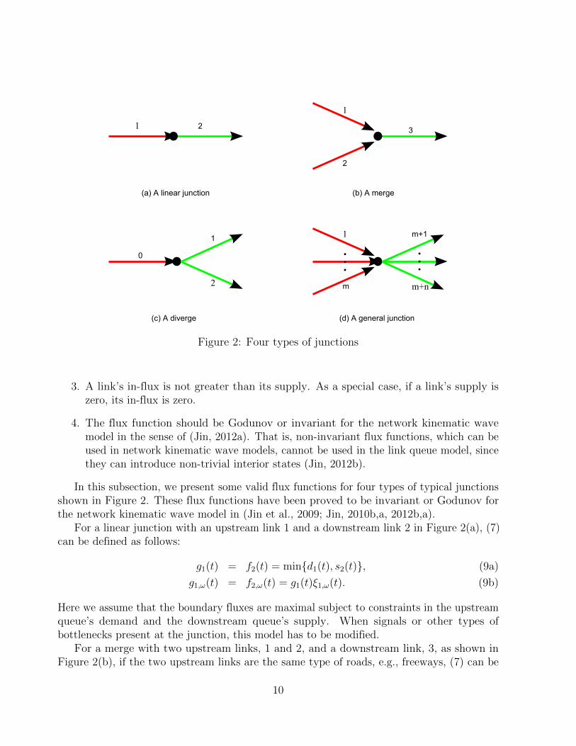
Figure 2: Four types of junctions

3. A link’s in-flux is not greater than its supply. As a special case, if a link’s supply iszero, its in-flux is zero.

4. The flux function should be Godunov or invariant for the network kinematic wavemodel in the sense of (Jin, 2012a). That is, non-invariant flux functions, which can beused in network kinematic wave models, cannot be used in the link queue model, sincethey can introduce non-trivial interior states (Jin, 2012b).

In this subsection, we present some valid flux functions for four types of typical junctionsshown in Figure 2. These flux functions have been proved to be invariant or Godunov forthe network kinematic wave model in (Jin et al., 2009; Jin, 2010b,a, 2012b,a).

For a linear junction with an upstream link 1 and a downstream link 2 in Figure 2(a), (7)can be defined as follows:

g1(t) = f2(t) = mind1(t), s2(t), (9a)

g1,ω(t) = f2,ω(t) = g1(t)ξ1,ω(t). (9b)

Here we assume that the boundary fluxes are maximal subject to constraints in the upstreamqueue’s demand and the downstream queue’s supply. When signals or other types ofbottlenecks present at the junction, this model has to be modified.

For a merge with two upstream links, 1 and 2, and a downstream link, 3, as shown inFigure 2(b), if the two upstream links are the same type of roads, e.g., freeways, (7) can be

10

defined by the fair merging rule:

f3(t) = mind1(t) + d2(t), s3(t), (10a)

g1(t) = mind1(t),maxs3(t)− d2(t),C1

C1 + C2

s3(t), (10b)

g2(t) = f3(t)− g1(t), (10c)

f3,ω(t) =2∑

a=1

ga(t)ξa,ω(t). (10d)

Note that the non-invariant fair merge model in (Jin and Zhang, 2003), g1(t) = mind1(t), s3(t) d1(t)d1(t)+d2(t)

,cannot be used in (7). If the two upstream links have different merging priorities; e.g., whenan on-ramp has a higher merging priority than a freeway, (7) can be defined as follows:

f3(t) = mind1(t) + d2(t), s3(t), (11a)

g1(t) = mind1(t),maxs3(t)− d2(t), αs3(t), (11b)

g2(t) = f3(t)− g1(t), (11c)

f3,ω(t) =2∑

a=1

ga(t)ξa,ω(t). (11d)

where α is the merging priority of link 1. Obviously the fair merging model is a special caseof the priority merging model.

For a diverge with an upstream link, 0, and two downstream links, 1 and 2, as shown inFigure 2(c), if all vehicles have pre-defined route choices and follow the FIFO diverging rule,(7) can be defined as follows:

g0(t) = mind0(t),s1(t)

ξ0→1(t),s2(t)

ξ0→2(t), (12a)

f1(t) = ξ0→1(t)g0(t), (12b)

f2(t) = ξ0→2(t)g0(t), (12c)

fa,ω(t) = g0(t)ξ0,ω(t), a = 1, 2, ω ∈ Ωa, ω ∈ Ω0. (12d)

where ξ0→1(t) =∑

ω∈Ω0∩Ω1ξ0,ω(t) and ξ0→2(t) =

∑ω∈Ω0∩Ω2

ξ0,ω(t) are the proportions ofvehicles on link 0 traveling to links 1 and 2, respectively. Here ξ0→1(t) ≥ 0, ξ0→2(t) ≥ 0,and ξ0→1(t) + ξ0→2(t) = 1. Again, the non-invariant diverge model in (Lebacque, 1996),f1(t) = minξ0→1(t)d0(t), s1(t), cannot be used in the link queue model. In emergencyevacuation situations, vehicles have no pre-defined route choices, (7) can be defined as follows:

g0(t) = mind0(t), s1(t) + s2(t), (13a)

f1(t) = mins1(t),maxd0(t)− s2(t), βd0(t), (13b)

f2(t) = g0(t)− f1(t), (13c)

11

where β is the evacuation priority of link 1.For a general junction j with m upstream links and n downstream links, as shown in

Figure 2(d), if all vehicles follow the FIFO diverging and fair merging rules, (7) can bedefined as follows (A→j = 1, · · · ,m and Aj→ = m+ 1, · · · ,m+ n):

1. From total and commodity densities on all links, ka(t) (a ∈ A→j), ka,ω(t) (a ∈ A→j,ω ∈ Ωa), kb(t) (b ∈ A←j), and kb,ω(t) (b ∈ A←j, ω ∈ Ωb), from (6) we can calculate allupstream demands, da(t) (a ∈ A→j), downstream supplies sb(t) (b ∈ Aj→), and theturning proportion ξa→b(t)

ξa→b(t) =∑

ω∈Ωa∩Ωb

ξa,ω(t), (14a)

where∑

b∈Aj→ ξa→b = 1 for a ∈ A→j . Note that origin demands and destination suppliescould be given as boundary conditions.

2. The out-flux of upstream link a ∈ A→j is

ga(t) = minda(t), θj(t)Ca, (14b)

where the critical demand level θj(t) uniquely solves the following min-max problem

θj(t) = min maxa∈A→j

da(t)Ca, min

b∈Aj→maxA1(t)

sb(t)−∑

α∈A→j\A1(t) dα(t)ξα→b(t)∑a∈A1(t) Caξa→b(t)

. (14c)

Here A1(t) a non-empty subset of A→j.

3. The commodity-flux is (a ∈ A→j, b ∈ Aj→, ω ∈ Ωa ∩ Ωb)

fb,ω(t) = ga,ω(t) = ga(t)ξa,ω(t). (14d)

4. The in-flux of downstream link b ∈ Aj→ is

fb(t) =∑a∈A→j

ga(t)ξa→b(t). (14e)

Since (9), (10), and (12) are its special cases, (14) is a unified junction flux function. Wehave the following observations on the unified junction model (14): (i) From (14e), in-and out-fluxes satisfy the conservation equations (2); (ii) The model satisfies the first-in-first-out (FIFO) diverging rule (Daganzo, 1995b), since the out-fluxes of an upstreamlink are proportional to the turning proportions; (iii) The model satisfies the fair mergingrule (Jin, 2010b), since, when all upstream links are congested, da(t) = Ca for a ∈ A→j,ga(t) = θj(t)Ca < Ca, and the total out-flux of link a is proportional to its capacity.

12

4 Analytical properties and numerical methods

In this section, we discuss the analytical properties and numerical methods for the link queuemodel. We also compare the model with existing models qualitatively.

4.1 Analytical properties

In this subsection we focus on the link queue model defined by (6), (8), and (14), wherevehicles have predefined routes and follow the fair merging and FIFO diverging rules. Thenwe obtain the following finite-dimensional link queue model:

dk(t)

dt= F(k(t),u(t); θθθ), (15)

where u(t) denote boundary conditions in origin demands or arrival rates and destinationsupplies, and θθθ include link lengths, fundamental diagrams, speed limits, metering rates,numbers of lanes, and other network and driver characteristics. In an extreme case withtriangular fundamental diagrams, if all links carry free flow, then (15) becomes a linearsystem and is therefore well-defined. Here we demonstrate that (15) is well-defined with (6)and (14) under general traffic conditions.

Lemma 4.1 The critical demand level in (14c) is well-defined: its solution exists and isunique. In addition, θj(t) ∈ [0, 1], and it is a continuous function of upstream demands,downstream supplies, and turning proportions.

Proof. Since the number of non-empty subsets of A→j is finite, the min-max problem in (14c)has a unique solution. Thus θj(t) has a unique solution for any combinations of upstreamdemands, downstream supplies, and turning proportions. Obviously it is a continuous function

in these variables. In addition, θj(t) ≥ 0, since maxA1(t)⊆A→jsb(t)−

∑α∈A→j\A1(t)

dα(t)ξα→b(t)∑a∈A1(t)

Caξa→b(t)≥

sb(t)∑a∈A→j(t)

Caξa→b(t)≥ 0. Since da(t) ≤ Ca from (6), we have θj(t) ∈ [0, 1].

Lemma 4.2 In (14), 0 ≤ ga(t) ≤ da(t), and 0 ≤ fb(t) ≤ sb(t). That is, in- and out-fluxesare bounded by the corresponding demands and supplies.

Proof. From (14b), we have 0 ≤ ga(t) ≤ da(t).

As shown in (Jin, 2012a), θj(t) = maxa∈A→jda(t)Ca

if and only if sb(t) ≥∑

a∈A→j da(t)ξa→b(t)

for all b; in this case, ga(t) = da(t), and fb(t) =∑

a∈A→j da(t)ξa→b(t) ≤ sb(t) for all b.Otherwise, there exists A∗ such that

θj(t) = minb∈Aj→

sb(t)−∑

α∈A→j\A∗ dα(t)ξα→b(t)∑a∈A∗ Caξa→b(t)

,

θj(t) <da(t)

Ca, a ∈ A∗

θj(t) ≥dα(t)

Cα, α ∈ A→j \ A∗

13

Then from (14b), we have ga(t) = θj(t)Ca for a ∈ A∗ and gα(t) = dα(t) for α ∈ A→j \ A∗.Thus for all b ∈ Aj→:

fb(t) = θj(t)∑a∈A∗

Caξa→b(t) +∑

α∈A→j\A∗

dα(t)ξα→b(t) ≤ sb(t).

Therefore 0 ≤ fb(t) ≤ sb(t).

Lemma 4.3 ga is a continuous function of da. In addition, it is piece-wise differentiable inda:

∂ga∂da

=

1, da ≤ θjCa0, da > θjCa

Therefore, ga is Lipschitz continuous in da. In addition, all out- and in-fluxes in (14) areLipschitz continuous in all upstream demands and downstream supplies.

Proof. Since θj is continuous in da, ga is also continuous in da. From properties of θj discussedin Section 4.3 of (Jin, 2012b), we can see that: (i) θj increases in da when da ≤ θjCa; (ii) when

da > θjCa, θj is constant at θ∗j = minb∈A←jsb−

∑α∈A→j\A∗1

dαξα→b∑a∈A∗1

Caξa→b, where a ∈ A∗1. Therefore,

when da ≤ θ∗jCa, from (14b) we have ga = da, and ∂ga∂da

= 1; when da > θ∗jCa, from (14b) we

have ga = θ∗jCa, and ∂ga∂da

= 0. Similarly, we can use properties of θj to prove that all out- andin-fluxes in (14) are Lipschitz continuous in all upstream demands and downstream supplies.

Theorem 4.4 The link queue model of network traffic flow, (8) together with (6) and (14),is well-defined. That is, under any given initial and boundary conditions, solutions to thesystem of ordinary differential equations (15) exist and are unique.

Proof. For general flow-density relations in fundamental diagrams, both traffic demand andsupply defined in (6) are Lipschitz continuous in traffic density. Further from Lemma (4.3),we can see that the right-hand side of (15) is Lipschitz continuous in all state variablesas well as boundary conditions. Then from the Picard-Lindelof theorem, solutions to thesystem of ordinary differential equations (15) exist and are unique under any given initialand boundary conditions (Coddington and Levinson, 1972). That is, the link queue model iswell-defined.

In summary, the link queue model, (15), has the following properties:

1. If a link is empty, from (6) its demand is zero, and its out-flux is zero. Thus from (8)the link’s density is always non-negative.

2. If a link is totally jammed, from (6) its supply is zero, and its in-flux equals zero. Thusfrom (8), the link’s density cannot increase after it reaches the jam density. Therefore,a normal link’s density is always bounded by its jam density.

14

3. In addition, a link’s out- and in-fluxes are bounded by its demand and supply, re-spectively. Since demand and supply are not greater than the capacity, the in- andout-fluxes are also bounded by road capacities.

4. At a junction, all related link queues interact with each other. Especially when adownstream link is congested, even if it is not totally jammed, the upstream links willbe impacted due to the limited supply provided by the downstream link. Therefore,queue spillbacks are automatically captured.

5. The information propagation speed on a link may not be finite, since traffic on a link isalways stationary instantaneously in a sense. Thus the model cannot capture shock orrarefaction waves inside a link.

6. For link a, the dynamic link flow-rate qa can be defined as qa = Qa(ka). But it is notused in the model, and may not be the same as the in-flux and out-flux, even when

traffic is stationary; i.e., when dka(t)

dt= 0. Thus link flow-rates are less important than

in- and out-fluxes in the model. Similarly, the link travel speed qa/ka is not explicitlyconsidered.

7. Since the link queue model is a system of ordinary differential equations, its solutions indensities, fluxes, and, therefore, travel times are all smooth (Coddington and Levinson,1972).

4.2 A numerical method

The link queue model, (15), cannot be analytically solved under general initial and boundaryconditions, but many numerical methods are available for finding its approximate solutions(Zwillinger, 1998). Here we present an explicit Euler method for the model. We discretizethe simulation time duration [0, T ] into M time steps with a time-step size of ∆t. At timestep i, the total and commodity densities on link a ∈ A′ are denoted by kia and kia,ω; Ki

o andKio,ω denote the numbers of vehicles, i.e., queue lengths. In addition, the boundary fluxes

during [i∆t, (i+ 1)∆t] are denoted by f ia, fia,ω, gia, and gia,ω.

On a normal link a, its demand, dia, and supply, sia, can be computed from kia with (6).For an origin link o, its demand can be computed as follows:

dio =Kio

∆t+ f ia. (16)

Then traffic states at time step i+ 1 can be updated with the discrete version of (15):

ki+1a = kia +

∆t

La(f ia − gia), (17a)

ki+1a,ω = kia,ω +

∆t

La(f ia,ω − gia,ω), (17b)

15

Ki+1o = Ki

o + (f io − gio)∆t, (17c)

Ki+1o,ω = Ki

o,ω + (f io,ω − gio,ω)∆t, (17d)

(17e)

where the boundary fluxes are computed by (14) with densities at time step i; i.e., at ajunction j, the boundary fluxes for all upstream links a ∈ A→j and downstream links b ∈ Aj→are given by

ξia→b =∑

ω∈Ωa∩Ωb

kia,ωkia

, (18a)

θij = min maxa∈A→j

diaCa, minb∈Aj→

maxAi1

sib −∑

α∈A→j\Ai1diαξ

iα→b∑

a∈Ai1Caξia→b

, (18b)

gia = mindia, θijCa, (18c)

f ib =∑a∈A→j

giaξia→b, (18d)

f ib,ω = gia,ω = giaξia,ω, (18e)

where Ai1 a non-empty subset of A→j. Here the arrival rates f io and f io,ω and destinationsupplies sir are given as boundary conditions. Note that, for an explicit Euler method, thetime step-size ∆t should be small enough for the discrete model, (17), to converge to thecontinuous version. In addition, the smaller ∆t, the closer are the numerical solutions totheoretical ones.

5 Comparison with existing models

In this section, we carefully compare the link queue model with existing link-based models aswell as kinematic wave models.

5.1 Comparison of qualitative properties and computational effi-ciency

Compared with existing link-based network loading models, the link queue model has thefollowing properties:

• The link queue model can be considered as an extension to the exit flow functionmodel, since out-fluxes are computed from link densities. However, in the link queuemodel, in-fluxes are also calculated from link densities, and both in- and out-fluxes aredetermined by densities of all links around a junction.

16

• In the link queue model, a point queue model is used for an origin link. But differentfrom the traditional point queue model, we define the demand in (6c), and the out-fluxis determined by the flux function (5) at the junction downstream to the origin queue.That is, the origin out-flux is determined by downstream links’ supplies when they’recongested. But in the traditional point queue model, interactions between a pointqueue and its downstream queues are not fully captured.

• The densities are bounded by jam-densities. That is, ka(t) ∈ [0, ka,j ] on a normal link a.

• Speed-density and flow-density relations are directly incorporated into the demand andsupply functions.

• At a junction, merging and diverging rules are included, and interactions among differentlinks are explicitly captured.

• The FIFO principle is automatically satisfied in such junction flux functions as (14).

• Link travel times can be calculated from in- and out-fluxes but are not included in themodel.

Compared with the network kinematic wave model (3), the link queue model, (8), canbe considered an approximation, since (i) fundamental diagrams of the kinematic wavemodel are used to calculate link demands and supplies and, therefore, in- and out-fluxes,and (ii) invariant flux functions of the kinematic wave model are used to calculate in- andout-fluxes through a junction. In addition, the discrete equations in (17) are highly relatedto the corresponding multi-commodity CTM when each link is discretized into only onecell. This also suggests the consistency between the link queue model and the kinematicwave model.2 From this relationship, we conclude that the time-step size, ∆t, in (17) shouldsatisfy the following CFL condition for all normal links (Courant et al., 1928), Va

∆tLa≤ 1;

i.e., ∆t ≤ mina∈A′LaVa

, where Va is the free-flow speed on link a. That is, the maximumtime-step size should not be greater than the smallest link traversal time in a network.However, different from the kinematic wave model, which is a system of infinite-dimensionalpartial differential equations, the link queue model is a system of finite-dimensional ordinarydifferential equations and cannot describe the formation, propagation, and dissipation ofshock and rarefaction waves on links. In a sense, in the link queue model, traffic is alwaysstationary on a link. Moreover, neither (17) or its continuous counterpart, (8), is equivalentto CTM: first, in (17), the solutions are more accurate with a smaller ∆t, but in CTM, ∆tshould be as big as possible so as to reduce numerical viscosities; second, in CTM, the cellsize, ∆x, should be small enough to capture the evolution of shock and rarefaction waves ona link, but in the link queue model, there is always one cell on a link.

Compared with the spatial queue and link transmission models, the link queue model alsoincorporates the concepts of linke demands and supplies and apply junction flux functions

2In a sense, CTMs can be considered cell queue models.

17

to determine links’ in- and out-fluxes. But the link queue model defines link demandsand supplies from link densities and is finite-dimensional. Therefore, it captures physicalcharacteristics of network traffic flow and remains mathematically tractable at the sametime.

In Table 1, we compare the computational efficiency, including both memory usage andcalculations, of the cell transmission, link transmission, and link queue models. In the table,∆x is the cell size, ∆t the time-step size, and Wa the shock wave speed in congested traffic.From the table, we have the following observations:

1. The state variable for the cell transmission model is infinite-dimensional, since it islocation dependent; but the other two models have a finite number of state variables.

2. Note that, in the cell transmission model, the cell size and the time-step size have tosatisfy the CFL condition: Va

∆t∆x≤ 1, where Va is the free-flow speed. In (Daganzo,

1995b), ∆x = Va∆t, which may not be always feasible in general road networks, butthe CTM has smaller numerical errors with larger CFL number Va

∆t∆x

(LeVeque, 2002).Therefore, when we decrease ∆t, we also need to decrease ∆x to obtain more accuratenumerical solutions in the cell transmission model.

3. In the cell transmission model, the number of state variables equals the number ofcells, La

∆x. Therefore, it increases when we decrease the cell size. Therefore the memory

usage is proportional to the number of cells. For the link transmission model, sincelink demands and supplies at time t are defined by fluxes at t − La

Vaand t − La

Wa,

respectively, fluxes between t − LaWa

, which is smaller than t − LaVa

, and t have to besaved in memory for fast retrieval. Therefore, the memory usage is proportional toLa

Wa∆t. Since Wa∆t < Va∆t ≈ ∆x, the memory usage of the link transmission model is

actually higher than that of the cell transmission model. But for the link queue model,we only need to save the current link density, and its memory usage is 1.

4. At each time step, the number of calculations is proportional the number of statevariables. Therefore, the cell transmission model needs more calculations, and thecalculation demand increases when we decrease ∆x.

Therefore we can see that the link queue model is much more efficient than both celltransmission and link transmission models.

5.2 Comparison with the kinematic wave model

In this subsection, we further compare the link queue model with the cell transmission andlink transmission models by numerical examples. Here all links share the following triangularfundamental diagram (Munjal et al., 1971; Haberman, 1977; Newell, 1993):

Qa(ka) = minVaka,Wa(nakj − ka) = min65ka, 2925na − 16.25ka),

18

State variables Memory usage Calculations per time stepCell Transmission ρa(xa, t)

La∆x

La∆x

Link Transmission fa(t), ga(t)La

Wa∆t2

Link Queue ka(t) 1 1

Table 1: Comparison of the computational efficiency per link among Cell Transmission, LinkTransmission, and Link Queue models

where na is the number of lanes, the free-flow speed Va = 65 mph, the jam density kj = 180vpmpl, and the shock wave speed in congested traffic Wa = 16.25 mph. Therefore, the criticaldensity ka,c = 36na, and

da = min65ka, 2340na,sa = min2925na − 16.25ka, 2340na.

5.2.1 Shock and rarefaction waves on one link

We consider a one-lane open road of one mile, La = 1, which is initially empty. The upstreamdemand is d−a = 2340 vph, and the downstream supply is s+

a = 1170 vph. In the kinematicwave model, either the cell transmission or link transmission model, the problem is solved bythe following: first, a rarefaction wave propagates the link with the critical density, 36 vpm,at the free flow speed, 65 mph. When the wave reached the downstream boundary at 1

65hr

or 55 s, a shock wave forms and travels upstream at the speed, Wa = 16.25. When the shockwave reaches the upstream at 1

65+ 1

16.25= 5

65hr or 277 s, the link reaches a stationary state

at ka = 108 vpm. Therefore the in- and out-fluxes are given by

fKWa (t) =

0, t < 02340, 0 ≤ t < 277 s,1170, t ≥ 277 s

gKWa (t) =

0, t < 55 s1170, t ≥ 277 s

In the link queue model, we have

dkadt

= minsa, 2340 −minda, 1170 = min2925− 16.25ka, 2340 −min65ka, 1170,

where ka(0) = 0. At t = 0, we have dkadt

= 2340, and ka increases. Until ka reaches 18 vpm, the

link queue model is equivalent to dkadt

= 2340−65ka, from which we have ka(t) = 36(1−e−65t)

for t ≤ t1 ≡ ln 265

. After t1 until ka reaches 36 vpm, the link queue model is equivalent todkadt

= 1170, and ka = 18 + 1170(t− t1) for t ≤ t2 ≡ t1 + 165

= ln 2+165

. After t2, the link queue

19

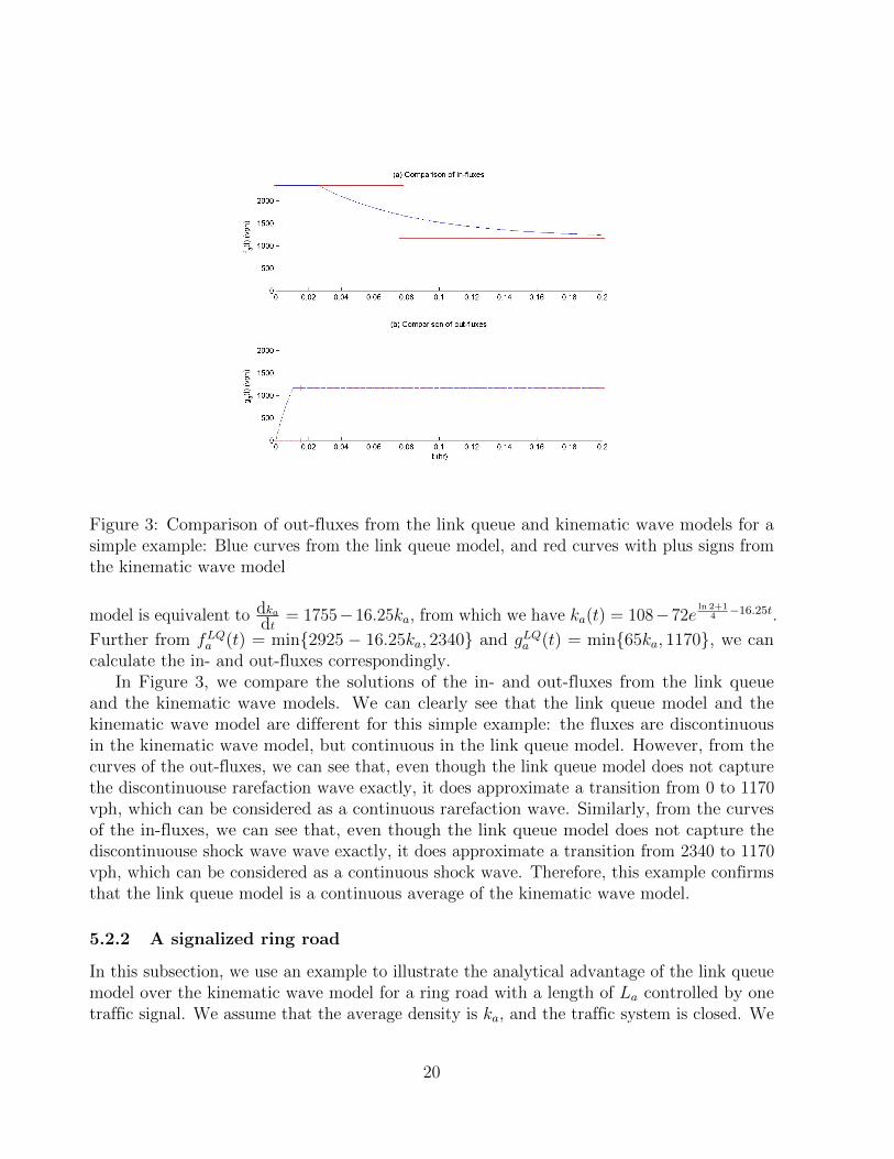
Figure 3: Comparison of out-fluxes from the link queue and kinematic wave models for asimple example: Blue curves from the link queue model, and red curves with plus signs fromthe kinematic wave model

model is equivalent to dkadt

= 1755−16.25ka, from which we have ka(t) = 108−72eln 2+1

4−16.25t.

Further from fLQa (t) = min2925 − 16.25ka, 2340 and gLQa (t) = min65ka, 1170, we cancalculate the in- and out-fluxes correspondingly.

In Figure 3, we compare the solutions of the in- and out-fluxes from the link queueand the kinematic wave models. We can clearly see that the link queue model and thekinematic wave model are different for this simple example: the fluxes are discontinuousin the kinematic wave model, but continuous in the link queue model. However, from thecurves of the out-fluxes, we can see that, even though the link queue model does not capturethe discontinuouse rarefaction wave exactly, it does approximate a transition from 0 to 1170vph, which can be considered as a continuous rarefaction wave. Similarly, from the curvesof the in-fluxes, we can see that, even though the link queue model does not capture thediscontinuouse shock wave wave exactly, it does approximate a transition from 2340 to 1170vph, which can be considered as a continuous shock wave. Therefore, this example confirmsthat the link queue model is a continuous average of the kinematic wave model.

5.2.2 A signalized ring road

In this subsection, we use an example to illustrate the analytical advantage of the link queuemodel over the kinematic wave model for a ring road with a length of La controlled by onetraffic signal. We assume that the average density is ka, and the traffic system is closed. We

20

introduce the signal function as

π(t) =

1 signal is green at t0 signal is red at t

(19)

If we consider the yellow signal, then π(t) can be a continuous function in t. But here weconsider effective green and effective red times. Usually π(t) is periodical; i.e., π(t+T ) = π(t).Assuming π is the green ratio. That is π is the average of π(t).

π =

∫ T0π(t)dt

T.

With the link queue model, we have

fa(t) = ga(t) = minda(t), sa(t)π(t) = π(t) minda(t), sa(t) = π(t)Qa(ka),

which is also periodical with period T . If we define the average flow-rate as fa =∫ T0 fa(t)dt

T,

then

fa = πQa(ka), (20)

which is a function of ka. This relationship is the macroscopic fundamental diagram for asignalized urban network (Godfrey, 1969; Daganzo and Geroliminis, 2008; Geroliminis andDaganzo, 2008). Note that this relationship is independent of the link length La and thesignal cycle length Π.

However, with the kinematic wave model, either the cell transmission or link transmissionmodel, the boundary fluxes cannot be easily calculated. In the following example, we considera ring road, whose length is 65

60miles. Thus the free-flow travel time on the link is 1 min.

At x = 0, we introduce a signal, whose cycle length is Π. We assume that the light is greenduring the first half of the signal, and red during the second half. When the ring road carriesa uniform initial density of 18 vpm, we apply the cell transmission model to simulate trafficdynamics for half an hour and demonstrate the solutions of fa(t) and ρa(x, t) for the lastfour cycles in Figure 4. In figures (a) and (b), the cycle length is 1 min; in figures (c) and(d), the cycle length is 2 min. Since the free-flow travel time is 1 min, when the cycle lengthis 1 min, the final traffic pattern alternates between zero density and critical density, asshown in Figure 4(b), and the boundary flux alternates between 0 and the capacity, as shownas shown in Figure 4(a). In this case, the average flux, fa, is about a half of the capacity.However, when the cycle length is 2 min, vehicles have to stop at the intersection as shownby the red regions in Figure 4(d), and the average flux, fa, is about a quarter of the capacity.With different densities and cycle lengths, then we are able to find the relationship betweenfa and ka, i.e., the macroscopic fundamental diagram for the cell transmission model.

In Figure 5, we demonstrate the macroscopic fundamental diagram, fa(ka), on a signalizedring road. In the figure, the green dashed curve is for the triangular fundamental diagram

21

Figure 4: Solutions of the cell transmission model for different cycle lengths: The dashedlines show the average fluxes in figures (a) and (c)

22

Figure 5: The macroscopic fundamental diagram of a signalized ring road

4 5

0 1

2

3

Figure 6: A diverge-merge network with one O-D pair and two intermediate links

without signal control, the red solid curve is the macroscopic fundamental diagram calculatedfrom the link queue model, (20), and the shaded region represents the macroscopic fundamentaldiagram calculated from the cell transmission model with different cycle lengths. This exampleagain confirms that the link queue model is a reasonable approximation of the kinematicwave model. In addition, this example also highlights the analytical simplicity of the linkqueue model, as the macroscopic fundamental diagram can be directly derived with thismodel.

6 The stability property of the link queue model

In this section, we apply the link queue model (15) to study traffic dynamics in a diverge-merge network with two intermediate links, referred to as the DM2 network, shown in Figure6. In the network, there are two commodities: vehicles of commodity 1 use link 1; and thoseof commodity 2 use link 2. We denote the dummy link at the origin by 4 and that at the

23

destination by 5. In this example, we do not consider the origin queue. Initially, the networkis empty: ka = 0 for a = 0, · · · , 3. Link lengths are La = 1, 1, 2, 1 miles for a = 0, · · · , 3,respectively; the number of lanes are na =3, 1, 2, 2, respectively. Here we assume thatvehicles follow the FIFO principle at the diverge and the fair merging rule at the merge.

6.1 Numerical results

We solve the link queue model with the numerical method in Section 4.2. The simulationtime duration is T = 1.05 hrs, and ∆t = 1.75 × 10−4 hrs, for which the CFL conditionis satisfied. To compare the results with those of the kinematic wave model (3), we alsosolve the commodity-based CTM with the same fundamental diagrams, demand and supplyfunctions, and merge and diverge models. For CTM, the cell size ∆x = 0.0125 miles, and thecorresponding CFL number vf

∆t∆x

= 0.91 < 1.We first compare the link queue model and the kinematic wave model with constant

loading patterns. Here the boundary conditions are constant: the origin demand is constantd4(t) = C0 = 7020 vph; the destination supply is also constant s5(t) = C3 = 4680 vph; andthe proportion of commodity 1 at the origin is ξ4,1 = ξ, where ξ is constant but can takethree different values: 0.3, 0.45, and 0.7. In (Jin, 2009), it was shown that the DM2 networkreaches damped periodic oscillatory, persistent periodic oscillatory, and stationary solutionsrespectively in these three cases. Since traffic dynamics are dictated by those on links 1 and2 in the network, in the following we only present link densities3, in- and out-fluxes on thesetwo links.

In Figure 7, we demonstrate the results from the link queue model and the kinematicwave model when ξ = 0.7 in the DM2 network. These figures confirm that, when ξ = 0.7,traffic reaches stationary states on links 1 and 2 eventually, since traffic densities reachconstant, and the in- and out-fluxes become equal on both links. We can observe the followingsimilarities between the two models:

• The two models have the same stationary states.

• On average the two models share the same dynamical patterns in densities, in- andout-fluxes.

• It takes a longer time for traffic to converge to stationary states on link 2 than on link1, since the former is longer.

We can also observe the following significant differences between the two models:

• Results from the link queue model converge in an exponential fashion, but those fromthe kinematic wave model converge in a finite time.

3In CTM, the link density equals the average value of all cell densities.

24

Figure 7: Comparison between the link queue and kinematic wave models when ξ = 0.7: Inall figures, the solid lines are results for the link queue model, and the dashed lines for thekinematic wave model; In figures (c) and (d), blue lines are for in-fluxes, and red lines forout-fluxes

25

Figure 8: Comparison between the link queue and kinematic wave models when ξ = 0.3: Inall figures, the solid lines are results for the link queue model, and the dashed lines for thekinematic wave model; In figures (c) and (d), blue lines are for in-fluxes, and red lines forout-fluxes

• In the link queue model, traffic densities and fluxes on both links become positiveimmediately after traffic is loaded at t > 0; but in the kinematic wave model, it takessome time for traffic densities and fluxes on both links to become positive, since it takestime for vehicles to travel from the origin to the diverging junction.

In Figure 8, we demonstrate the results from the two models when ξ = 0.3. The dashedcurves in figures (c) and (d) confirm that damped periodic oscillations occur on both links.But results from the link queue still converge to stationary states exponentially. In Figure9, we demonstrate the results from the two models when ξ = 0.45. The dashed curves inall figures confirm that persistent periodic oscillations occur on both links. The period isabout 0.2 hours or 12 minutes. 4 In both cases, results from the link queue still exponentiallyconverge to stationary states, but the results from the link queue model are still consistentwith those from the kinematic wave model on average.

We then compare the link queue model and the kinematic wave model with a varying

4In (Jin, 2009), it was shown that the period is determined by the lengths of links 1 and 2 as well as thecorresponding fundamental diagrams.

26

Figure 9: Comparison between the link queue and kinematic wave models when ξ = 0.45: Inall figures, the solid lines are results for the link queue model, and the dashed lines for thekinematic wave model; In figures (c) and (d), blue lines are for in-fluxes, and red lines forout-fluxes

27

Figure 10: Comparison between the link queue and kinematic wave models with varyingdemand patterns when ξ = 0.45: In all figures, the solid lines are results for the link queuemodel, and the dashed lines for the kinematic wave model; In figures (c) and (d), blue linesare for in-fluxes, and red lines for out-fluxes

loading pattern: the origin demand is periodic d4(t) = 12C0(sin(4πt/T ) + 1) vph, where

T = 1.05 hrs; the destination supply is still constant s5(t) = C3 = 4680 vph; and theproportion of commodity 1 at the origin is ξ4,1 = 0.45, which leads to persistent periodicoscillations with constant demands in the preceding subsection. Still, we only compare linkdensities, in- and out-fluxes on the two intermediate links.

In Figure 10, we demonstrate the results from the two models. We can see that trafficdynamics on the network are dominated by the varying demand pattern. The dashed curvein all figures show that persistent periodic oscillations occur on both links when the trafficdemand is higher than a certain level, and the period is still about 12 minutes. Clearly, evenwith varying demand patterns, the link queue model is still consistent with the kinematicwave model in the simulation results.

6.2 Theoretical analysis of the stability property

In (Jin, 2013), it was shown that the kinematic wave model for the diverge-merge networkcan be unstable when one intermediate link is congested, but the other not. Based on theobservation of circular information propagation, a Poincare map was derived and used to

28

characterize the stability and bifurcation property of the kinematic wave model. In particular,for the network shown in Figure 6 with constant loading patterns as in the precedingsubsection and ξ ∈ (1

3, 1

2), links 1 and 2 can be stationary at SUC and SOC, respectively, but

the stationary state is unstable, and persistent periodic oscillatory traffic patterns can occur,as shown in Figure 9.

In this subsection, we analytically prove that the link queue model is always stable forξ ∈ (1

3, 1

2). Since in the stationary state links 1 and 2 are stationary at SUC and SOC,

respectively, from (12) we have f1(t) = ξ1−ξs2(t), and f2(t) = s2(t); from (10) we have

g1(t) = d1(t), and g2(t) = C3 − d1(t). Note that d1(t) is an increasing function in k1(t) infree-flow traffic, and s2(t) is a decreasing function in k2(t) in congested traffic. Then the linkqueue model can be simplified as

dk1(t)

dt=

1

L1

(ξ

1− ξs2(t)− d1(t)) ≡ F1(k1, k2), (21a)

dk2(t)

dt=

1

L2

(s2(t) + d1(t)− C3) ≡ F2(k1, k2). (21b)

Then the Jacobian matrix of the nonlinear system of ordinary differential equations is

∇F =

[ ∂F1

∂k1

∂F1

∂k2∂F2

∂k1

∂F2

∂k2

]=

[−a ξ

1−ξ b

a b

],

where a = dd1dk1

> 0 and b = ds2dk2

< 0. We denote the eigenvalue by λ. Then the characteristic

equation is λ2+(a−b)λ− 11−ξab = 0. Since λ1+λ2 = −(a−b) < 0 and λ1λ2 = − 1

1−ξab > 0, the

real parts of both eigenvalues are negative, and the link queue model, (21), is asymptoticallystable at the stationary states.

This analysis can be easily extended to demonstrate the stability of the link queuemodel for (DM)n networks studied in (Jin, 2013). Therefore the link queue model, (15), isalways stable for network traffic flow, and the stability property of the link queue model isfundamentally different from that of the kinematic wave model.

7 Conclusions

In this paper, we presented a link queue model of network traffic flow, in which the evolutionof congestion levels on a road link is described by changes in the link density. With linkdemands and supplies, it can capture basic characteristics of link traffic flow, includingcapacity, free-flow speed, jam density, and so on. In addition, with appropriate junction fluxfunctions, it can describe the initiation, propagation, and dissipation of traffic queues in aroad network caused by merging, diverging, and other network bottlenecks.

Compared with existing link-based models, the link queue model rigorously describeinteractions among different links by using link demands, supplies, and junction models

29

consistent with macroscopic merging and diverging behaviors. Therefore, the link queuemodel is physically more meaningful.

Compared with the kinematic wave model, including its cell transmission and linktransmission formulations, the link queue model has the following properties:

1. As a system of ordinary differential equations, the link queue model is finite-dimensional,but the kinematic wave model are infinite-dimensional, either as partial differentialequations (cell transmission) or delay differential equations (link transmission).

2. The link queue model is always stable, but the kinematic wave model may not be, asdemonstrated in Section 6 both analytically and numerically.

3. The link queue model is computationally more efficient than the cell transmission andlink transmission models, as shown in Table 1.

4. The boundary fluxes in the link queue model are continuous in time, but those in thekinematic wave model can be discontinuous with shock waves, as demonstrated inSection 5.2.1 and Section 6.1.

5. The link queue model is analytically more tractable, as demonstrated in Section 5.2.2for a signalized ring road.

6. The link queue model has the same stationary states as the kinematic wave model, asthey share the same fundamental diagrams for the same links and the same macroscopicmerging and diverging rules. In particular, interactions among link flows at a junction,including queue spillbacks, are described in both models.

7. The dynamic solutions of the link queue model approximate those of the kinematicwave model for different networks with constant or variable demand patterns, asdemonstrated in Sections 5.2 and 6.1.

Therefore, the link queue model is fundamentally different from the kinematic wave model,including the cell transmission and link transmission formulations, even though the linkqueue model is extended from the latter. However, the link queue model captures the mostimportant two characteristics of network traffic flow, namely static fundamental diagramsand dynamic junction models, and is a continuous and stable approximation of the kinematicwave model in a large-scale road network during a time period in the order of 10 minutes.

From this study, we can see that the link queue model indeed fills the gap betweenthe kinematic wave model and traditional link-based models, as it is not as detailed as thekinematic wave model but is still physically meanginful in a large spatial-temporal domain,but the new model is more mathematically tractable than the more detailed kinematic wavemodel. Therefore, the link queue model is a useful addition to the multiscale modelingframework of network traffic flow. In applications, we may first apply the link queue modelto obtain analytical insights of network congestion patterns under different demand levels,

30

control strategies, route choice behaviors, or other conditions and then apply the kinematicwave model as well as microscopic models to further study the propagation of traffic queuesand other details before drawing any conclusions or making any policy recommendations.

In the future we will be interested in developing link queue models of other traffic flowsystems, which are consistent with kinematic wave models:

• If commodity flows are not explicitly tracked, but the turning proportions ξa→b(t) atall junctions can be detected through loop detectors or other devices, we can obtain alink queue model of implicit multi-commodity traffic. In this case, only one equation,(1a), is needed for the evolution of total traffic on a link; (14b,c,e) can still be used tocalculate in- and out-fluxes at a junction; and fb,ω(t) and ga,ω(t) are not available in(14d). This model is suitable for traffic operations when route choice behaviors are notexplicitly accounted for.

• If a network is closed without any origin or destination links, the link queue model canstill be applied. In this case, turning proportions at all junctions can be exogeneousor endogenous, and the model becomes an autonomous system without boundaryconditions in origin demands or destination supplies.

• The model can be extended for multi-class, multi-lane-group traffic systems with lane-changing traffic, HOV lanes, traffic signals, capacity drops, ramp metering, etc. Themajor challenge is to define traffic demands and supplies in (6) and extend the junctionflux functions in (14) for such scenarios.

With the link queue model, we will also be interested in studying the following problemspertaining to network traffic flow: (i) stationary states, or equilibria, of the link queuemodel in open or closed networks (Jin, 2012c); (ii) hybrid link queue, kinematic wave, andcar-following models; (iii) analyses and simulations of traffic dynamics in a large-scale roadnetwork with data input. In addition, the link queue model, (15), can be viewed as a controlsystem, in which u are control variables. From the viewpoint of control systems, we cananalyze the system’s responses to control signals, and many transportation applications canbe studied as control problems. Furthermore, since the link queue model is always stable andhas continuous arrival and departure flows, it could be encapsulated to more mathematicallytractable and numerically efficient formulations of the dynamic traffic assignment problem(Lo, 1999).

References

Astarita, V., 1996. A continuous time link model for dynamic network loading based ontravel time function. Proceedings of the 13th International Symposium on Transportationand Traffic Theory, 79--102.

31

Beckmann, M., 1952. A continuous model of transportation. Econometrica: Journal of theEconometric Society 20 (4), 643--660.

Boyce, D., Mahmassani, H., Nagurney, A., 2005. A retrospective on Beckmann, McGuire,and Winstens Studies in the Economics of Transportation. Papers in Regional Science84 (1), 85--103.

Carey, M., 1986. A constraint qualification for a dynamic traffic assignment model. Trans-portation Science 20 (1), 55--58.

Carey, M., 2004. Link travel times ii: properties derived from traffic-flow models. Networksand Spatial Economics 4 (4), 379--402.

Carey, M., Ge, Y., 2007. Retaining desirable properties in discretising a travel-time model.Transportation Research Part B 41 (5), 540--553.

Coddington, E., Levinson, N., 1972. Theory of ordinary differential equations. Tata McGraw-Hill Education.

Courant, R., Friedrichs, K., Lewy, H., 1928. Uber die partiellen Differenzengleichungen dermathematischen Physik. Mathematische Annalen 100, 32--74.

Daganzo, C. F., 1995a. Properties of link travel time functions under dynamic loads. Trans-portation Research Part B 29 (2), 95--98.

Daganzo, C. F., 1995b. The cell transmission model II: Network traffic. TransportationResearch Part B 29 (2), 79--93.

Daganzo, C. F., 1996. The nature of freeway gridlock and how to prevent it. Proceedings ofthe 13th International Symposium on Transportation and Traffic Theory, 629--646.

Daganzo, C. F., 2006. On the variational theory of traffic flow: well-posedness, duality andapplications. Networks and Heterogeneous Media 1 (4), 601--619.

Daganzo, C. F., Geroliminis, N., 2008. An analytical approximation for the macroscopicfundamental diagram of urban traffic. Transportation Research Part B 42 (9), 771--781.

Del Castillo, J. M., Benitez, F. G., 1995. On the functional form of the speed-densityrelationship - II: Empirical investigation. Transportation Research Part B 29 (5), 391--406.

Drissi-Kaıtouni, O., Hameda-Benchekroun, A., 1992. A dynamic traffic assignment modeland a solution algorithm. Transportation Science 26 (2), 119--128.

Friesz, T., Bernstein, D., Smith, T., Tobin, R., Wie, B., 1993. A variational inequalityformulation of the dynamic network user equilibrium problem. Operations Research 41 (1),179--191.

Friesz, T., Luque, J., Tobin, R., Wie, B., 1989. Dynamic Network Traffic AssignmentConsidered as a Continuous Time Optimal Control Problem. Operations Research 37 (6),893--901.

Garavello, M., Piccoli, B., 2006. Traffic Flow on Networks. Vol. 1. Applied MathematicsSeries.

Gazis, D., Herman, R., Potts, R., 1959. Car-following theory of steady-state traffic flow.Operations Research 7 (4), 499--505.

Gazis, D. C., Herman, R., Rothery, R. W., 1961. Nonlinear follow-the-leader models of trafficflow. Operations Research 9 (4), 545--567.

32

Geroliminis, N., Daganzo, C. F., 2008. Existence of urban-scale macroscopic fundamentaldiagrams: Some experimental findings. Transportation Research Part B 42 (9), 759--770.

Gipps, P. G., 1986. A model for the structure of lane changing decisions. TransportationResearch Part B 20 (5), 403--414.

Godfrey, J., 1969. The mechanism of a road network. Traffic Engineering and Control 8 (8),323--327.

Greenshields, B. D., 1935. A study in highway capacity. Highway Research Board Proceedings14, 448--477.

Haberman, R., 1977. Mathematical models. Prentice Hall, Englewood Cliffs, NJ.Herman, R., Prigogine, I., 1979. A two-fluid approach to town traffic. Science 204 (4389),

148--151.Hidas, P., 2005. Modelling vehicle interactions in microscopic simulation of merging and

weaving. Transportation Research Part C 13 (1), 37--62.Ho, H., Wong, S., 2006. Two-dimensional continuum modeling approach to transportation

problems. Journal of Transportation Systems Engineering and Information Technology6 (6), 53--68.

Jin, W.-L., 2009. Asymptotic traffic dynamics arising in diverge-merge networks with twointermediate links. Transportation Research Part B 43 (5), 575--595.

Jin, W.-L., 2010a. Analysis of kinematic waves arising in diverging traffic flow models. Arxivpreprint.URL http://arxiv.org/abs/1009.4950

Jin, W.-L., 2010b. Continuous kinematic wave models of merging traffic flow. TransportationResearch Part B 44 (8-9), 1084--1103.

Jin, W.-L., 2012a. A Riemann solver for a system of hyperbolic conservation laws at a generalroad junction. Arxiv preprint.URL http://arxiv.org/abs/1204.6727

Jin, W.-L., 2012b. A kinematic wave theory of multi-commodity network traffic flow. Trans-portation Research Part B 46 (8), 1000--1022.

Jin, W.-L., 2012c. The traffic statics problem in a road network. Transportation ResearchPart B 46 (10), 13601373.

Jin, W.-L., 2013. Stability and bifurcation in network traffic flow: A Poincare map approach.URL http://arxiv.org/abs/1307.7671

Jin, W.-L., Chen, L., Puckett, E. G., 2009. Supply-demand diagrams and a new frameworkfor analyzing the inhomogeneous Lighthill-Whitham-Richards model. Proceedings of the18th International Symposium on Transportation and Traffic Theory, 603--635.

Jin, W.-L., Zhang, H. M., 2003. On the distribution schemes for determining flows through amerge. Transportation Research Part B 37 (6), 521--540.

Kerner, B., Konhauser, P., 1993. Cluster effect in initially homogeneous traffic flow. PhysicalReview E 48 (4), 2335--2338.

Kulkarni, V., 1997. Fluid models for single buffer systems. Frontiers in Queueing: Modelsand Applications in Science and Engineering, 321--338.

33

Kuwahara, M., Akamatsu, T., 1997. Decomposition of the reactive dynamic assignmentswith queues for a many-to-many origin-destination pattern. Transportation Research PartB 31 (1), 1--10.

Lebacque, J. P., 1996. The Godunov scheme and what it means for first order traffic flowmodels. Proceedings of the 13th International Symposium on Transportation and TrafficTheory, 647--678.

LeVeque, R. J., 2002. Finite volume methods for hyperbolic problems. Cambridge UniversityPress, Cambridge; New York.

Lighthill, M. J., Whitham, G. B., 1955. On kinematic waves: II. A theory of traffic flow onlong crowded roads. Proceedings of the Royal Society of London A 229 (1178), 317--345.

Lo, H., 1999. A dynamic traffic assignment formulation that encapsulates the cell transmissionmodel. Proceedings of the 14th International Symposium on Transportation and TrafficTheory, 327--350.

Merchant, D., Nemhauser, G., 1978. A model and an algorithm for the dynamic trafficassignment problems. Transportation Science 12 (3), 183--199.

Munjal, P. K., Hsu, Y. S., Lawrence, R. L., 1971. Analysis and validation of lane-drop effectsof multilane freeways. Transportation Research 5 (4), 257--266.

Nagel, K., Schreckenberg, M., 1992. A cellular automaton model for freeway traffic. Journalde Physique I France 2 (2), 2221--2229.

Newell, G., 1982. Applications of queueing theory. Vol. 733. Chapman and Hall New York.Newell, G. F., 1993. A simplified theory of kinematic waves in highway traffic I: General

theory. II: Queuing at freeway bottlenecks. III: Multi-destination flows. TransportationResearch Part B 27 (4), 281--313.

Ni, D., 2011. Multiscale modeling of traffic flow. Mathematica Aeterna 1 (1), 27--54.Nie, X., Zhang, H., 2002. The Formulation of A Link Based Dynamic Network Loading

Model Considering Queue Spillovers. Tech. rep., working Paper UCD-ITS-Zhang-2002-6.Nie, X., Zhang, H., 2005. Delay-function-based link models: their properties and computa-

tional issues. Transportation Research Part B 39 (8), 729--751.Osorio, C., Flotterod, G., Bierlaire, M., 2011. Dynamic network loading: A stochastic

differentiable model that derives link state distributions. Transportation Research Part B45 (9), 1410--1423.

Payne, H. J., 1971. Models of freeway traffic and control. Simulation Councils ProceedingsSeries: Mathematical Models of Public Systems 1 (1), 51--61.

Peeta, S., Ziliaskopoulos, A., 2001. Foundations of Dynamic Traffic Assignment: The Past,the Present and the Future. Networks and Spatial Economics 1 (3), 233--265.

Prigogine, I., Herman, R., 1971. Kinetic theory of vehicular traffic. American Elsevier.Richards, P. I., 1956. Shock waves on the highway. Operations Research 4 (1), 42--51.Treiterer, J., Myers, J., 1974. The hysteresis phenomenon in traffic flow. Proceedings of the

Sixth International Symposium on Transportation and Traffic Theory, 13.Vickrey, W. S., May 1969. Congestion theory and transport investment. The American

Economic Review: Papers and Proceedings of the Eighty-first Annual Meeting of the

34

American Economic Association 59 (2), 251--260.Wardrop, J. G., 1952. Some theoretical aspects of road traffic research. Proceedings of the

Institute of Civil Engineers 1 (3), 325--378.Whitham, G. B., 1974. Linear and nonlinear waves. John Wiley and Sons, New York.Yperman, I., Logghe, S., Tampere, C., Immers, B., 2006. The Multi-Commodity Link

Transmission Model for Dynamic Network Loading. Proceedings of the TRB AnnualMeeting.

Zhang, H. M., Nie, Y., 2005. Modeling network flow with and without link interactions:properties and implications. In: Proceedings of the 84th TRB Annual Meeting.

Zwillinger, D., 1998. Handbook of differential equations. Academic Press.

35