The Pennsylvania State University

The Graduate School

Department of Mathematics

A LINEAR SHELL THEORY

BASED ON VARIATIONAL PRINCIPLES

A Thesis in

Mathematics

by

Sheng Zhang

c© 2001 Sheng Zhang

Submitted in Partial Fulfillmentof the Requirements

for the Degree of

Doctor of Philosophy

August 2001

We approve the thesis of Sheng Zhang.

Date of Signature

Douglas N. ArnoldDistinguished Professor of MathematicsThesis AdviserChair of Committee

M. Carme CaldererProfessor of Mathematics

Chun LiuAssistant Professor of Mathematics

Eduard S. VentselProfessor of Engineering Science and Mechanics

Gary L. MullenProfessor of MathematicsChair, Department of Mathematics

iii

Abstract

Under the guidance of variational principles, we derive a two-dimensional shell

model, which is a close variant of the classical Naghdi model. From the model solution,

approximate stress and displacement fields can be explicitly reconstructed. Convergence

of the approximate fields toward the more accurate three-dimensional elasticity solutions

is proved. Convergence rates are established. Potential superiority of the Naghdi-type

model over the Koiter model is addressed. The condition under which the model might

fail is also discussed.

iv

Table of Contents

List of Figures . . . . . . . . . . . . . . . . . . . . . . . . . . . . . . . . . . . . . ix

Acknowledgments . . . . . . . . . . . . . . . . . . . . . . . . . . . . . . . . . . . x

Chapter 1. Introduction . . . . . . . . . . . . . . . . . . . . . . . . . . . . . . . . 1

1.1 Background and motivations . . . . . . . . . . . . . . . . . . . . . . . 1

1.2 Organization of this thesis . . . . . . . . . . . . . . . . . . . . . . . . 5

1.3 Principal results . . . . . . . . . . . . . . . . . . . . . . . . . . . . . . 7

1.3.1 Plane strain cylindrical shells . . . . . . . . . . . . . . . . . . 8

1.3.2 Spherical shells . . . . . . . . . . . . . . . . . . . . . . . . . . 10

1.3.3 General shells . . . . . . . . . . . . . . . . . . . . . . . . . . . 12

Chapter 2. Plane strain cylindrical shell model . . . . . . . . . . . . . . . . . . . 19

2.1 Introduction . . . . . . . . . . . . . . . . . . . . . . . . . . . . . . . . 19

2.2 Plane strain cylindrical shells . . . . . . . . . . . . . . . . . . . . . . 20

2.2.1 Curvilinear coordinates on a plane domain . . . . . . . . . . . 21

2.2.2 Plane strain elasticity . . . . . . . . . . . . . . . . . . . . . . 22

2.2.3 Plane strain cylindrical shells . . . . . . . . . . . . . . . . . . 25

2.2.4 Rescaled stress and displacement components . . . . . . . . . 29

2.3 The shell model . . . . . . . . . . . . . . . . . . . . . . . . . . . . . . 32

2.4 Reconstruction of the stress and displacement fields . . . . . . . . . . 37

2.4.1 Reconstruction of the statically admissible stress field . . . . 37

v

2.4.2 Reconstruction of the kinematically admissible displacement

field . . . . . . . . . . . . . . . . . . . . . . . . . . . . . . . . 40

2.4.3 Constitutive residual . . . . . . . . . . . . . . . . . . . . . . . 41

2.5 Justification . . . . . . . . . . . . . . . . . . . . . . . . . . . . . . . . 44

2.5.1 Assumption on the applied forces . . . . . . . . . . . . . . . . 44

2.5.2 An abstract theory . . . . . . . . . . . . . . . . . . . . . . . . 45

2.5.3 Asymptotic behavior of the model solution . . . . . . . . . . 47

2.5.4 Convergence theorem . . . . . . . . . . . . . . . . . . . . . . . 54

2.6 Shear dominated shell examples . . . . . . . . . . . . . . . . . . . . . 60

2.6.1 A beam problem . . . . . . . . . . . . . . . . . . . . . . . . . 60

2.6.2 A circular cylindrical shell problem . . . . . . . . . . . . . . . 62

Chapter 3. Analysis of the parameter dependent variational problems . . . . . . 65

3.1 Introduction . . . . . . . . . . . . . . . . . . . . . . . . . . . . . . . . 65

3.2 The parameter dependent problem and its mixed formulation . . . . 65

3.3 Asymptotic behavior of the solution . . . . . . . . . . . . . . . . . . 72

3.3.1 The case of surjective membrane–shear operator . . . . . . . 74

3.3.2 The case of flexural domination . . . . . . . . . . . . . . . . . 78

3.3.3 The case of membrane–shear domination . . . . . . . . . . . . 83

3.4 Parameter-dependent loading functional . . . . . . . . . . . . . . . . 90

3.5 Classification . . . . . . . . . . . . . . . . . . . . . . . . . . . . . . . 95

Chapter 4. Three-dimensional shells . . . . . . . . . . . . . . . . . . . . . . . . . 96

4.1 Curvilinear coordinates on a shell . . . . . . . . . . . . . . . . . . . . 96

vi

4.2 Linearized elasticity theory . . . . . . . . . . . . . . . . . . . . . . . 106

4.3 Rescaled components . . . . . . . . . . . . . . . . . . . . . . . . . . . 109

Chapter 5. Spherical shell model . . . . . . . . . . . . . . . . . . . . . . . . . . . 115

5.1 Introduction . . . . . . . . . . . . . . . . . . . . . . . . . . . . . . . . 115

5.2 Three-dimensional spherical shells . . . . . . . . . . . . . . . . . . . . 116

5.3 The spherical shell model . . . . . . . . . . . . . . . . . . . . . . . . 120

5.4 Reconstruction of the admissible stress and displacement fields . . . 124

5.4.1 The admissible stress and displacement fields . . . . . . . . . 125

5.4.2 The constitutive residual . . . . . . . . . . . . . . . . . . . . . 129

5.5 Justification . . . . . . . . . . . . . . . . . . . . . . . . . . . . . . . . 131

5.5.1 Assumption on the applied forces . . . . . . . . . . . . . . . . 131

5.5.2 Asymptotic behavior of the model solution . . . . . . . . . . 132

5.5.3 Convergence theorem . . . . . . . . . . . . . . . . . . . . . . . 139

5.5.4 About the condition of the convergence theorem . . . . . . . 144

5.5.5 A shell example for which the model might fail . . . . . . . . 146

Chapter 6. General shell theory . . . . . . . . . . . . . . . . . . . . . . . . . . . 148

6.1 Introduction . . . . . . . . . . . . . . . . . . . . . . . . . . . . . . . . 148

6.2 The shell model . . . . . . . . . . . . . . . . . . . . . . . . . . . . . . 150

6.3 Reconstruction of the stress field and displacement field . . . . . . . 155

6.3.1 The stress and displacement fields . . . . . . . . . . . . . . . 156

6.3.2 The second membrane stress moment . . . . . . . . . . . . . 160

6.3.3 The integration identity . . . . . . . . . . . . . . . . . . . . . 164

vii

6.3.4 Constitutive residual . . . . . . . . . . . . . . . . . . . . . . . 169

6.3.5 A Korn-type inequality on three-dimensional thin shells . . . 172

6.4 Classification . . . . . . . . . . . . . . . . . . . . . . . . . . . . . . . 174

6.4.1 Assumptions on the loading functions . . . . . . . . . . . . . 174

6.4.2 Classification . . . . . . . . . . . . . . . . . . . . . . . . . . . 175

6.5 Flexural shells . . . . . . . . . . . . . . . . . . . . . . . . . . . . . . . 178

6.5.1 Asymptotic behavior of the model solution . . . . . . . . . . 179

6.5.2 Convergence theorems . . . . . . . . . . . . . . . . . . . . . . 183

6.5.3 Plate bending . . . . . . . . . . . . . . . . . . . . . . . . . . . 188

6.6 Totally clamped elliptic shells . . . . . . . . . . . . . . . . . . . . . . 189

6.6.1 Reformulation of the resultant loading functional . . . . . . . 192

6.6.2 Asymptotic behavior of the model solution . . . . . . . . . . 194

6.6.3 Convergence theorems . . . . . . . . . . . . . . . . . . . . . . 197

6.6.4 Estimates of the K-functional for smooth data . . . . . . . . 198

6.7 Membrane–shear shells . . . . . . . . . . . . . . . . . . . . . . . . . . 204

6.7.1 Asymptotic behavior of the model solution . . . . . . . . . . 205

6.7.2 Admissible applied forces . . . . . . . . . . . . . . . . . . . . 213

6.7.3 Convergence theorem . . . . . . . . . . . . . . . . . . . . . . . 216

Chapter 7. Discussions and justifications of other linear shell models . . . . . . . 222

7.1 Negligibility of the higher order term in the loading functional . . . . 223

7.2 The Naghdi model . . . . . . . . . . . . . . . . . . . . . . . . . . . . 226

7.3 The Koiter model and the Budianski–Sanders model . . . . . . . . . 227

viii

7.4 The limiting models . . . . . . . . . . . . . . . . . . . . . . . . . . . 230

7.5 About the loading assumption . . . . . . . . . . . . . . . . . . . . . . 232

7.6 Concluding remarks . . . . . . . . . . . . . . . . . . . . . . . . . . . 234

References . . . . . . . . . . . . . . . . . . . . . . . . . . . . . . . . . . . . . . . . 235

ix

List of Figures

2.1 A cylindrical shell and its cross section . . . . . . . . . . . . . . . . . . . 27

2.2 Deformations of a cylindrical shell . . . . . . . . . . . . . . . . . . . . . 50

2.3 Shear dominated deformation of a beam . . . . . . . . . . . . . . . . . . 60

2.4 Shear dominated deformation of a circular cylinder . . . . . . . . . . . . 62

4.1 A shell and its coordinate domain . . . . . . . . . . . . . . . . . . . . . . 105

x

Acknowledgments

I am most grateful and indebted to my thesis advisor, Prof. Douglas N. Arnold,

for his advice that led to my selection of the project, his penetrating vision that guided me

moving forward, his enthusiasm toward mathematics that made me feel the mathematical

research somewhat enjoyable, and for his patience, encouragement, and support.

I wish to thank Professors M. Carme Calderer, Chun Liu, and Eduard S. Ventsel

who kindly agreed to serve on my thesis committee.

During the writing of this thesis, I was supported by the Pritchard Dissertation

Fellowship, which is gratefully acknowledged.

1

Chapter 1

Introduction

1.1 Background and motivations

A shell is a three-dimensional elastic body occupying a thin neighborhood of a

two-dimensional manifold, which resists deformation owing to the material of which it

is made, its shape, and boundary conditions. It is extremely important in structural

mechanics and engineering because a well-designed shell can sustain large loads with

remarkably little material. For example, before collapsing, a totally clamped spherical

shell of thickness 2 ε can hold a strain energy of O(ε−1/3) times that which can be

tolerated by a flat plate of the same thickness (see page 202). For this reason, shells are

a favored structural element in both natural and man-made constructions. While elastic

shells can exhibit great strength, their behaviors can also be very difficult to predict,

and they can fail in a catastrophic fashion.

Although the deformation of a shell arising in response to given loads and bound-

ary conditions can be accurately captured by solving the three-dimensional elasticity

equations, shell theory attempts to provide a two-dimensional representation of the in-

trinsically three-dimensional phenomenon [34]. There are two reasons to derive a lower

dimensional model. One is its simpler mathematical structure. For example, the ex-

istence, regularity, bifurcation, and global analysis are by now on firm mathematical

2

grounds for non-linear elastic rods [18]. In contrast, the mathematical theory for non-

linear three-dimensional elasticity is much less developed. Another motivation is for

numerical simulation. An accurate, fully three-dimensional, simulation of a very thin

body is beyond the power of even the most powerful computers and computational

techniques. Furthermore, the standard methods of numerical approximation of three-

dimensional elastic bodies fail for bodies which are thin in some direction, unless the

behavior is resolved in that direction. Thus the need for two-dimensional shell models

[5].

Beginning in the late nineteenth century, and especially during the past few

decades, there have been intense efforts to derive an accurate dimensionally reduced

mathematical theory of shells. Despite much progress, the development of a satisfac-

tory mathematical theory of elastic shells is far from complete. The methodologies for

deriving shell models from three-dimensional continuum theories are still being devel-

oped, and the relation between different approaches, are not clear. Controversial issues

abound. The extremely important question of deriving rigorous mathematical theory

relating shell models to more exact three-dimensional models is wide open. A thorough

analysis of the mathematical models derived and a rigorous definition of their ranges of

applicability is mostly lacking.

There is a huge literature devoted to dimensional reduction in elasticity theory.

Several classical approaches are employed in investigations. One approach starts with a

priori assumptions on the displacement and stress fields based on mechanical consider-

ations, such as the Kirchhoff–Love assumption on the displacements and the kinetic as-

sumption on the stress fields that assumes both the transverse shear and normal stresses

3

are negligible. This approach leads to the biharmonic plate bending model, Koiter shell

model, flexural shell model, and many others. Models derived in this way have proved

successful in practice, but this approach does not seem to lend itself naturally to an error

analysis [2].

Another approach is through a formal asymptotic analysis in which the thickness

of the elastic body is viewed as a small parameter. By expanding the three-dimensional

elasticity equation with respect to the thickness, the leading terms in the expansion

are used to define lower dimensional models. This approach leads to limiting models

describing the zero thickness limit situation, among which are the limiting flexural and

membrane models, depending on ad hoc assumptions on the applied forces, the shell

geometry, and boundary conditions. These asymptotic methods only lead to the limiting

models. It does not seem to be possible to derive the better Koiter and Naghdi models

by this approach. (Taking more terms in the asymptotic expansion does not lead to a

dimensionally reduced model.) See [18] for a comprehensive treatment of this approach.

A third approach is by variational methods. Solution of the three-dimensional

equation can be characterized by variational principles or weak formulations. An ap-

proximation is determined by restricting to a trial space of functions that are finite

dimensional with respect to the transverse variable. By its very nature, this approach

leads to models that yield a displacement field or a stress field determined by finitely

many functions of two variables. Thus the dimension is reduced. In this approach, the

two energies principle, or the Prager–Synge theorem [54], plays a fundamental role in

the model validation. To apply the two energies principle, we must have a statically

admissible stress field and a kinematically admissible displacement field. The latter is

4

usually easy to come by, but the former might be formidable to obtain. The two energies

principle is particularly suited to analyzing complementary energy variational models,

which automatically yield statically admissible stress fields.

The application of the two energies principle to justify plate theory was initiated

in the pioneering work of Morgenstern [47], where it was used to prove the convergence

of the biharmonic model of plate bending when the thickness tends to zero. The stat-

ically admissible stress field and the kinematically admissible displacement field were

constructed based on the biharmonic solution in an ad hoc fashion, as needed for the

convergence proof. Following this work, substantial efforts have been made to modify

the justification of the classical plate bending models, see [48], [51], and [57]. In the

same spirit, Gol’denveizer [29], Sensenig [56], Koiter [33], Mathuna [46], and many oth-

ers considered the error estimates for shell theories. In these latter works, the stress

fields constructed from the model solutions were only approximately admissible, and the

justifications obtained were largely formal.

Due to the formidable difficulty involved in the construction of an admissible stress

field based on the solution of a known model, it seems a better choice to reconsider the

derivation of the model while keeping in mind the construction of the statically admissible

stress field as a primary goal. Based on the Hellinger–Reissner variational formulations

of the three-dimensional elasticity, a systematic procedure of dimensional reduction for

plate problems was developed in [2]. In this approach both the stress and displacement

fields were restricted to subspaces in which functions depend on the transverse coordinate

polynomially. The derivation based on the second Hellinger–Reissner principle not only

led to the well known Reissner–Mindlin plate model but also furnished an admissible

5

stress field and so naturally led to a rigorous justification of the model by the two

energies principle. This approach is not easily extensible to shell problems. Due to the

curved shape of a shell, if this approach were carried over and the subspaces were chosen

to be composed of functions depending on the transverse coordinate polynomially, the

polynomials would be of conspicuously higher order. The resulting model would contain

so many unknowns that it would be nearly as untractable as the three-dimensional model.

In this work we derive and rigorously justify a two-dimensional shell model guided

by the variational principles.

1.2 Organization of this thesis

We consider the modeling of the deformation arising in response to applied forces

and boundary conditions of an arbitrary thin curved shell, which is made of isotropic

and homogeneous elastic material whose Lame coefficients are λ and µ. The shell is

clamped on a part of its lateral face and is loaded by a surface force on the remaining

part of the lateral face. The shell is subjected to surface tractions on the upper and

lower surfaces and loaded by a body force. We take the three-dimensional linearized

elasticity equation as the supermodel and approximate it by a two-dimensional model.

The lower dimensional model will be justified by proving convergence and establishing the

convergence rate of the model solution to the solution of the three-dimensional elasticity

equation in the relative energy norm under some assumptions on the applied forces.

Conditions under which the model might fail will be discussed. The two energies principle

supplies important guidance for the construction of the model.

6

Throughout the thesis, Greek subscripts and superscripts, except ε, which is re-

served for the half-thickness of the shell, always take their values in 1, 2, while Latin

scripts always belong to the set 1, 2, 3. Summation convention with respect to repeated

superscripts and subscripts will be used together with these rules. We usually use lower

case Latin letters with an undertilde, as v∼, to denote two-dimensional vectors. Lower case

Greek letters with double undertildes denote two-dimensional second order tensors, as

σ∼∼. However, the fundamental forms on the shell middle surface will be denoted by lower

case Latin letters. We use boldface Latin letters to denote three-dimensional vectors and

boldface Greek letters second order three-dimensional tensors. Vectors and tensors will

be given in terms of their covariant components, or contravariant components, or mixed

components.

The notation P ' Q means there exist constants C1 and C2 independent of ε, P ,

and Q such that C1P ≤ Q ≤ C2P . The notation P . Q means there exists a constant

C independent of ε, P , and Q such that P ≤ CQ.

Chapters 2–6 form the main body of the thesis, with Chapters 2 and 5 treating

two special kinds of shells, namely, the plane strain cylindrical shells and spherical shells,

respectively; Chapter 6 treating general shells; and Chapters 3 and 4 containing results

needed for the analysis. The reason we treat cylindrical and spherical shells separately is

that for these special shell problems, we can construct statically admissible stress fields

and kinematically admissible displacement fields, so that we can use the two energies

principle to justify the models by bounding the constitutive residuals. As a consequence,

stronger convergence results can be obtained for these cases. These two special shells

provide examples for all kinds of shells as classified in Section 3.5. For the general

7

shells treated in Chapter 6, precisely admissible stress fields are no longer possible to

construct. The derivation yields an almost admissible stress field with small residuals

in the equilibrium equation and lateral traction boundary condition. The two energies

principle can not be directly used to justify the model. As an alternative, we establish

an integration identity to incorporate all these residuals so that we can bound the model

error by estimating these residuals.

All the models we derive can be written in variational forms, in which the flexural

energy, membrane energy, and shear energy are combined together in the total strain

energy. Contributions of the component energies are weighted by factors that depend

on ε. Chapter 3 is devoted to the mathematical analysis of such ε-dependent problems

on an abstract level. In this chapter, we classify the model and analyze the asymptotic

behavior of the model solution when the shell thickness approaches zero. The range

of applicability of the derived model will also be discussed on the abstract level. The

rigorous validation of the shell model crucially hinges on these analyses.

In Chapter 4, we briefly summarize the three-dimensional linearized elasticity the-

ory expressed in the curvilinear coordinates on a thin shell. We also derive some formulas

that can substantially simplify calculations. Finally, in Chapter 7, we will discuss the

relations between our theory and other existing shell theories. In the remainder of this

introduction, we will describe the principal results of the following chapters.

1.3 Principal results

In this section we summerize the key results of Chapters 2, 5, and 6.

8

1.3.1 Plane strain cylindrical shells

In Chapter 2 we consider the simplest case of plane strain cylindrical shells. In

this case, the three-dimensional problem is essentially a two-dimensional problem defined

on a cross-section, so the dimensionally reduced model should be one-dimensional. We

assume that the cylindrical shell is clamped on the two lateral sides, subjected to surface

forces on the upper and lower surfaces, and loaded by a body force.

Let the middle curve of a cross-section of the cylindrical shell be parameterized

by its arc length variable x ∈ [0, L]. Our model can be written as a one-dimensional

variational problem defined on the space H = [H10(0, L)]3. The solution of the model is

composed of three single variable functions that approximately describe the shell defor-

mation arising in response to the applied forces and boundary conditions. We introduce

the following operators. For any (θ, u,w) ∈ H, we define

γ(u,w) = ∂u− bw, ρ(θ, u,w) = ∂θ + b(∂u− bw), τ(θ, u,w) = θ + ∂w + bu,

which give the membrane strain, flexural strain, and transverse shear strain engendered

by the displacement functions (θ, u,w). Here b is the curvature of the middle curve,

which is a function of the arc length parameter, and ∂ = d/dx.

The model (cf., (2.3.2) below) reads: Find (θε, uε, wε) ∈ H, such that

13ε2(2µ + λ?)

∫ L

0ρ(θε, uε, wε)ρ(φ, y, z)dx

9

+ (2µ + λ?)∫ L

0γ(uε,wε)γ(y, z)dx +

56µ

∫ L

0τ(θε, uε, wε)τ(φ, y, z)dx

= 〈f0 + ε2 f1, (φ, y, z)〉, ∀(φ, y, z) ∈ H,

in which

λ? =2µλ

2µ+ λ

and the loading functional f0+ε2 f1 is explicitly expressible in terms of the applied force

functions, cf., (2.3.3), (2.3.4). We show that the solution of this one-dimensional model

uniquely exists. The three single variable functions θε, uε, and wε that comprise the

model solution describe the rotations of straight fibers normal to the middle curve, the

tangential displacements, and transverse displacements of points on the middle curve,

respectively.

In addition to the model, in Section 2.4 we give formulae to reconstruct a tensor

field σ∼∼ and a vector field v∼ from the model solution on the shell cross-section, see

equations (2.4.1), (2.4.3), (2.4.7), and (2.4.8). The model and reconstruction formulae

are designed to have the following properties:

(1) σ∼∼ is a statically admissible stress field (see Section 2.4.1).

(2) v∼ is a kinematically admissible displacement field (see Section 2.4.2).

(3) The terms of leading order in ε in the constitutive residual Aαβλγσλγ−χαβ(v∼)

vanish, so the constitutive residual may be shown to be small as ε→ 0 (see Section 2.4.3).

10

This allows a bound on the errors of σ∼∼ and v∼ by the two energies principle. Under

the loading assumptions (2.3.6) and (2.5.1), we prove the inequality

‖σ∼∼∗ − σ∼∼‖Eε + ‖χ∼∼(v∼

∗)− χ∼∼(v∼)‖Eε‖χ∼∼(v∼)‖Eε

. ε1/2,

in which σ∼∼∗ is the stress field and v∼

∗ the displacement field arising in the shell determined

from the two-dimensional elasticity equations. The norm ‖ · ‖Eε is the energy norm of

the strain or stress field.

1.3.2 Spherical shells

For spherical shells, we derive the model by a similar method. We assume the

middle surface of the shell is a portion of a sphere of radius R. The shell is clamped

on a part of its lateral face, and subjected to surface force on the remaining part of the

lateral face whose density is linearly dependent on the transverse variable. The shell

is subjected to surface forces on the upper and lower surfaces, and loaded by a body

force whose density is assumed to be constant in the transverse coordinate. The middle

surface is parameterized by a mapping from a domain ω ⊂ R2 onto it. The boundary

∂ω is divided as ∂ω = ∂Dω ∪ ∂Tω giving the clamping and traction parts of the the

lateral face of the shell. The model is a two-dimensional variational problem defined on

the space H = H∼1D(ω)×H∼

1D(ω)×H1

D(ω). The solution of the model is composed of five

two variable functions that can approximately describe the shell displacement arising in

11

response to the applied loads and boundary conditions. For (θ∼, u∼, w) ∈ H, we define

γαβ(u∼, w) =12

(uα|β + uβ|α)− baαβw,

ραβ(θ∼) =12

(θα|β + θβ|α), τβ(θ∼, u∼, w) = θβ + ∂βw + buβ,

which give the membrane, flexural, and transverse shear strains engendered by the dis-

placement functions (θ∼, u∼, w). Here, aαβ is the covariant metric tensor and b = −1/R is

the curvature of the middle surface. The model (cf., (5.3.2)) reads: Find (θ∼ε, u∼

ε, wε) ∈

H, such that

13ε2∫ωaαβλγρλγ(θ∼

ε)ραβ(φ∼)√adx∼

+∫ωaαβλγγλγ(u∼

ε, wε)γαβ(v∼, z)√adx∼+

56µ

∫ωaαβτβ(θ∼

ε, u∼ε, wε)τα(φ∼, v∼, z)

√adx∼

= 〈f0 + ε2 f1, (φ∼, y∼, z)〉, ∀ (φ∼, y∼, z) ∈ H

where aαβ is the contravariant metric tensor of the middle surface and

aαβλγ = 2µaαλaβγ + λ?aαβaλγ (1.3.1)

is the two-dimensional elasticity tensor of the shell. The resultant loading functional

f0 + ε2 f1 can be explicitly expressed in terms of the applied force functions, cf., (5.3.3),

(5.3.4). This model has a unique solution if the resultant loading functional is in the dual

space of H. This condition is satisfied if the applied force functions satisfy the condition

(5.3.6). The unique solution (θ∼ε, u∼

ε, wε) describes the normal straight fiber rotations,

12

middle surface tangential displacement and transverse displacement, respectively. A

statically admissible stress field and a kinematically admissible displacement field can

be reconstructed from the model solution. We prove the convergence and establish the

convergence rate of the model solution to the three-dimensional solution by estimating

the constitutive residual.

1.3.3 General shells

For a general shell, except for some smoothness requirements, we do not impose

any restriction on the geometry of the shell middle surface or the shape of its lateral

boundary. The shell is assumed to be clamped on a part of its lateral surface and loaded

by a surface force on the remaining part. The shell is subjected to surface forces on the

upper and lower surfaces, and loaded by a body force.

The model is constructed in the vein of the model constructions for the special

shells in the Chapters 2 and 5. The main difficulty to overcome is that our model

derivation does not yield a statically admissible stress field. Therefore, the two energies

principle can not be directly used to justify the model. Even so, we can reconstruct a

stress field that is almost admissible with small residuals in the equilibrium equation

and lateral traction boundary condition. And we will establish an integration identity

(6.3.17) to incorporate the equilibrium residual and the lateral traction boundary con-

dition residual. This identity plays the role of the two energies principle in the general

shell theory.

Let the middle surface of the shell be parameterized by a mapping from the domain

ω ⊂ R2 onto it. Corresponding to the clamping and traction parts of the lateral face,

13

the boundary of ω is divided as ∂ω = ∂Dω ∪ ∂T ω. In this curvilinear coordinates, the

fundamental forms on the shell middle surface are denoted by aαβ , bαβ , and cαβ . The

mixed curvature tensor is denoted by bαβ . The model is a two-dimensional variational

problem defined on the space H = H∼1D(ω) × H∼

1D(ω) × H1

D(ω). The solution of the

model is composed of five two variable functions that can approximately describe the

shell displacement arising in response to the applied loads and boundary conditions. For

(θ∼, u∼, w) ∈ H, we define the following two-dimensional tensors.

γαβ(u∼, w) =12

(uα|β + uβ|α)− bαβw,

ραβ(θ∼, u∼, w) =12

(θα|β + θβ|α) +12

(bλβuα|λ + bλαuβ|λ)− cαβw,

τβ(θ∼, u∼, w) = bλβuλ + θβ + ∂βw.

These two-dimensional tensor- and vector-valued functions give the membrane strain,

flexural strain, and transverse shear strain engendered by the displacement functions

(θ∼, u∼, w), respectively. The model (cf., (6.2.4)) reads: Find (θ∼ε, u∼

ε, wε) ∈ H, such that

13ε2∫ωaαβλγρλγ(θ∼

ε, u∼ε, wε)ραβ(φ∼, y∼, z)

√adx∼

+∫ωaαβλγγλγ(u∼

ε, wε)γαβ(y∼, z)√adx∼+

56µ

∫ωaαβτβ(θ∼

ε, u∼ε, wε)τα(φ∼, y∼, z)

√adx∼

= 〈f0 + ε2 f1, (φ∼, y∼, z)〉, ∀(φ∼, y∼, z) ∈ H,

in which the fourth order two-dimensional contravariant tensor aαβλγ is the elastic tensor

of the shell, defined by the formula (1.3.1). The resultant loading functional f0 + ε2 f1

14

can be explicitly expressed in terms of the applied force functions, cf., (6.2.5), (6.2.6).

This model has a unique solution if the resultant loading functional is in the dual space of

H, a condition that can be easily satisfied. From the model solution, we can reconstruct

a stress field σ by explicitly giving its contravariant components. By a correction to

the transverse deflection, we can define a displacement field v by giving its covariant

components. Under some conditions, we will prove the convergence of both σ and v

to the stress and displacement fields determined from the three-dimensional elasticity

equation by using the aforementioned identity and bounding the constitutive residual,

equilibrium equation residual and lateral traction boundary condition residual.

The model is a close variant of the classical Naghdi shell model. This model differs

from the generally accepted Naghdi model in three ways. First, the resultant loading

functional has a somewhat more involved form. Second, the coefficient of the shear

term is 5/6 rather than the usual value 1. The “best” choice for this coefficient seems an

unresolved issue for shells. When the shell is flat, the model degenerates to the Reissner–

Mindlin plate bending and stretching models for which the corresponding value 5/6 is

often accepted as the best, see [55] and [2]. The third, and most significant, difference

is in the expression of the flexural strain ραβ . The relation between our definition and

that of Naghdi’s (ρNαβ) is

ραβ = ρNαβ + bλαγλβ + bγβγγα.

We will see that the change of the flexural strain expression appears to be necessary to

make the constitutive residual small in some cases (see Remark 6.3.2). In most cases, this

15

difference does not affect the convergence of the model solution to the three-dimensional

solution.

When the general shell model is applied to spherical shells, we obtain a spherical

shell model slightly different from what we derived in Chapter 5 both in the form of the

flexural strain and in the resultant loading functional. The convergence properties of

these two spherical shell models are the same. What we can learn from this discrepancy

is that the model can be changed, but the resultant loading functional must be changed

accordingly, otherwise a variation in the form of a model might lead to divergence.

To prove convergence, we need to make an assumption on the dependence of the

applied force functions on the shell thickness. We will assume that all the applied force

functions that are explicitly involved in the resultant loading functional are independent

of ε. Under this assumption, by properly defining function spaces and operators, the

shell models can be abstracted to the variational problem:

ε2(Au,Av)U + (Bu,Bv)V = 〈f0 + ε2 f1, v〉H∗×H,

u ∈ H, ∀ v ∈ H,

(1.3.2)

where H, U , and V are Hilbert spaces. The functionals f0 and f1 are independent of ε.

The linear bounded operators A and B are from H to U and V respectively, with the

property

‖Au‖2U + ‖Bu‖2V ' ‖u‖2H ∀ u ∈ H.

We can assume that the range W of the operator B is dense in V , and equip W with

a norm to make it a Hilbert space. For the plane strain cylindrical shell model, we

16

can prove that the operator B has closed range. This special property substantially

simplifies the analysis of behavior of the model solution and significantly strengthes the

convergence results.

The asymptotic behavior of the solution of this abstract problem is mostly deter-

mined by the leading term f0 in the loading functional. We classify the problem as a

flexural shell problem if f0|kerB 6= 0. For flexural shells, after scaling the applied forces,

the model can be viewed as the penalization of the limiting flexural shell model, which is

constrained on kerB and independent of ε. The behavior of the model solution and its

convergence property to the three-dimensional solution crucially hinge on the regularity

of the Lagrange multiplier ξ0 of this constrained limiting problem. Without any extra

assumption, we have ξ0 ∈W ∗ and the convergence

limε→0

‖σ∗ − σ‖Eε + ‖χ(v∗)− χ(v)‖Eε‖χ(v)‖Eε

= 0, (1.3.3)

in which σ∗ is the stress field and v∗ is the displacement field determined from the three-

dimensional elasticity. The norm is the energy norm and χ(v) is the three-dimensional

strain field engendered by the displacement v.

The convergence rate essentially depends on the position of ξ0 between V ∗ and

W ∗. Under the assumption (6.5.14), we can prove the inequality

‖σ∗ − σ‖Eε + ‖χ(v∗)− χ(v)‖Eε‖χ(v)‖Eε

. εθ, (1.3.4)

17

in which θ ∈ [0, 1]. Note that the case of θ = 0 corresponds to the situation that ξ0 is

only in W ∗. The previous convergence result can not be deduced from this result on the

convergence rate.

If f0|kerB = 0, by the closed range theorem in functional analysis, there exists a

unique ζ0∗ ∈ W ∗ such that the leading term of the resultant loading functional can be

reformulated as

〈f0, v〉H∗×H = 〈ζ0∗ , Bv〉W ∗×W ∀ v ∈ H.

If we only have ζ0∗ ∈ W ∗, we can not prove any convergence. Very likely, the model

diverges in the energy norm in this case. If ζ0∗ ∈ V ∗, the abstract problem will be called

a membrane–shear problem. This condition is a necessary requirement for us to prove the

convergence of the model solution to the three-dimensional solution. Under this condition

and the assumption that the applied forces are admissible (the admissible assumption on

the applied forces is not needed for spherical shells), we can prove a convergence of the

form (1.3.3). The convergence rate is determined by where ζ0, the Riesz representation

of ζ0∗ in V , stands between W and V . For a totally clamped elliptic shell, which is a

special example of membrane–shear shells, under some smoothness assumption on the

shell data in the Sobolev sense, we prove the convergence rate

‖σ∗ − σ‖Eε + ‖χ(v∗)− χ(v)‖Eε‖χ(v)‖Eε

. ε1/6 .

If the odd part of the tangential surface forces vanishes, the convergence rate O(ε1/5)

can be proved.

18

The condition ζ0∗ ∈ V ∗ is essentially equivalent to the existence condition for a

solution of the “generalized membrane” shell model defined in [18]. This condition is

trivially satisfied for shear dominated plane strain cylindrical shells. For shear dominated

plate bending, the condition is satisfied as long as the loading function belongs to L2.

The condition is acceptable for stiff parabolic shells and stiff hyperbolic shells. It can

be satisfied for a totally clamped elliptic shell if the shell data are fairly smooth in the

Sobolev sense. But it imposes a stringent restriction for a partially clamped elliptic shell,

in which case even if the shell data are infinitely smooth, the condition might not be

satisfied. If the condition is not satisfied, although the model solution always exists, a

rigorous relation to the three-dimensional solution is completely lacking.

To reveal the potential advantages of using the Naghdi-type model, we need a

different assumption on the applied force functions. Specifically, we assume that the odd

part of the applied surface forces has a bigger magnitude than what usually assumed.

Under this assumption and in the convergent case of membrane–shear shells, the model

solution violates the Kirchhoff–Love hypothesis on which the Koiter shell model were

based. Therefore it can not converge.

Finally, in the last chapter, we give justifications for other linear shell models

based on the convergence theorems proved for the general shell model, and we will show

that under the usual loading assumption, the differences between our model and other

models are not significant.

For lack of space, we excluded the model derivations. We will directly present the

models and address the more important issue of rigorous justifications.

19

Chapter 2

Plane strain cylindrical shell model

2.1 Introduction

The shell problem of this chapter is a special example of general shells. The

mathematical structure of the derived model is much simpler and we can get much

stronger results on the model convergence. Although the problem is simple, it reveals

our basic strategy to tackle the general problem.

We consider a 3D elastic body that is an infinitely long cylinder whose cross

section is a curvilinear thin rectangle. The body is clamped on the two lateral sides and

subjected to surface traction forces on the upper and lower surfaces and loaded by a

body force. The applied forces are assumed to be in the sectional plane. Under these

assumptions, the elasticity problem is a plane strain problem and can be fully described

by a 2D problem defined on a cross section. We assume that the width 2 ε of the sectional

curvilinear rectangle is much smaller than its length, so the cylinder is a thin shell.

When the shell is thin, it is reasonable to approximately reduce the 2D elasticity

problem to a 1D problem defined on the middle curve of a cross section. A system of

ordinary differential equations defined on the middle curve that can effectively capture

the displacement and stress of the shell arising in response to the applied forces and

boundary conditions will be the desired shell model.

20

The model, which is a close variant of the Naghdi shell model, is constructed

under the guidance of the two energies principle. The plane strain elasticity problem

and the two energies principle will be briefly described in section 2.2. The model will be

presented and the existence and uniqueness of its solution will be proved in Section 2.3.

We reconstruct the admissible stress and displacement fields from the model solution

and compute the constitutive residual in Section 2.4. In Section 2.5, we analyze the

asymptotic behavior of the model solution and prove the convergence theorem.

Our conclusion is that when the limiting flexural model has a nonzero solution,

our model solution converges to the exact solution at the rate of ε1/2 in the relative

energy norm. In this case, the model is just as good as the limiting flexural model and

Koiter model. When the solution of the limiting flexural model is zero, our model gives

a solution that can capture the membrane and shear deformations, and the convergence

rate in the relative energy norm is still ε1/2. The non-vanishing transverse shear defor-

mation violates the Kirchhoff–Love hypothesis in this case. Finally, to emphasize the

necessity of using the Naghdi-type model in some cases, we give two examples in which

the deformations are shear-dominated, which can be very well captured by our model,

but is totally missed by the limiting flexural model and the Koiter model.

2.2 Plane strain cylindrical shells

Since the cross section of the cylindrical shell is a curvilinear rectangle, it is

advantageous to work with curvilinear coordinates. In this section we briefly describe

the plane strain elasticity theory in curvilinear coordinates for a cylindrical shell.

21

2.2.1 Curvilinear coordinates on a plane domain

Let ω ⊂ R2 be an open domain, and (x1, x2) be the Cartesian coordinates of a

generic point in it. Let Φ : ω → R2 be an injective mapping. We assume that Ω = Φ(ω)

is a connected open domain and ∂Ω = Φ(∂ω). The pair of numbers (x1, x2) then

furnish the curvilinear coordinates on Ω. At any point along the coordinate lines, the

tangential vectors gα = ∂Φ/∂xα form the covariant basis. The covariant components

gαβ of the metric tensor are given by gαβ = gα ·gβ. The contravariant basis vectors are

determined by the relation gα · gβ = δαβ . The contravariant components of the metric

tensor are gαβ = gα · gβ . Note that gαλgλβ = δαβ . The Christoffel symbols are defined

by Γ∗λαβ = gλ · ∂βgα.

Any vector field v∼ defined on Ω can be expressed in terms of its covariant com-

ponents vα or contravariant components vα by v∼ = vαgα = vαgα. Any second-order

tensor field σ∼∼ can be expressed in terms of its contravariant σαβ or covariant components

σαβ by σ∼∼ = σαβgα ⊗ gβ = σαβgα ⊗ gβ.

The covariant derivative, a second order tensor field, of a vector field v∼ is defined

in terms of covariant components by

vα‖β = ∂βvα − Γ∗λαβvλ, (2.2.1)

which is the gradient of the vector field.

The covariant derivative of a tensor field with contravariant components σαβ is

defined by

σαβ‖λ = ∂λσαβ + Γ∗αλγσ

γβ + Γ∗βλγσαγ, (2.2.2)

22

which are mixed components of a third order tensor field. The row divergence of the

tensor field σαβ is a vector field resulting from a contraction of this third order tensor,

div σ∼∼ = σαβ‖β = ∂βσαβ + Γ∗αβγσ

βγ + Γ∗ββγσαγ. (2.2.3)

The components of a vector or tensor field defined over Ω can be viewed as functions

defined on the coordinate domain ω.

2.2.2 Plane strain elasticity

Let an infinitely long cylindrical elastic body occupying the 3D domain Ω ×

(−∞,∞) ⊂ R3 be clamped on a part of its surface ∂DΩ× (−∞,∞). On the remaining

part of the surface ∂TΩ× (−∞,∞), the body is subjected to the surface traction force

whose density p∼ is in the Ω-plane and independent of the longitudinal direction. If the

applied body force q∼ is also assumed to be in the Ω-plane and independent of the longi-

tudinal direction, the displacement of the body arising in response to the applied forces

and clamping boundary condition will be in the plane of Ω and constant in the longitudi-

nal direction. The displacement can be represented by a 2D vector field v∼ and the strain

by a 2D tensor field χ∼∼ defined on Ω. The stress field can also be treated as a 2D tensor

field σ∼∼ that is composed of the in-plane components. Although the stress component

in the direction normal to the Ω-plane does not vanish, it is totally determined by the

in-plane stress components.

23

The following five equations (2.2.4–2.2.8) constitute the theory of plane strain

elasticity. The theory includes the geometric equation

χαβ(v∼) =12

(vα‖β + vβ‖α) (2.2.4)

and the constitutive equation

σαβ = Cαβλγχλγ, or χαβ = Aαβλγσλγ, (2.2.5)

where the fourth order tensors Cαβλγ and Aαβλγ are the plane strain elasticity tensor

and the compliance tensor respectively, given by

Cαβλγ = 2µgαλgβγ + λgαβgλγ

and

Aαβλγ =1

2µ[gαλgβγ −

λ

2(µ + λ)gαβgλγ ],

in which λ and µ are the Lame coefficients of the elastic material comprising the cylinder.

To describe the equilibrium equation and boundary conditions, we need more notations.

We denote the unit outward normal on the boundary ∂Ω by n∼ = nαgα. Let the surface

force density be p∼ = pαgα, and body force density be q∼ = qαgα. With these notations,

the equilibrium equation can be written as

σαβ‖β + qα = 0. (2.2.6)

24

On the part of the domain boundary ∂TΩ, the surface force condition can be expressed

as

σαβnβ = pα. (2.2.7)

On ∂DΩ, the body is clamped, so the condition is

vα = 0. (2.2.8)

According to the linearized elasticity theory, the system of equations (2.2.4),

(2.2.5), (2.2.6) together with the boundary conditions (2.2.7) and (2.2.8) uniquely de-

termine the covariant components v∗α of the displacement field of the elastic body

arising in response to the applied forces and the prescribed clamping boundary con-

dition. The stress distribution σ∼∼∗ is determined by giving its contravariant components

σ∗αβ = Cαβλγχλγ(v∼∗).

The weak formulation of the plane strain elasticity equation is

∫ΩCαβλγχλγ(v∼)χαβ(u∼) =

∫Ωqαuα +

∫∂TΩ

pαuα,

v∼ ∈ H∼1D(ω) ∀ u∼ ∈ H∼

1D(ω),

(2.2.9)

in which H∼1D(ω) is the space of vector-valued functions that are square integrable and

have square integrable first derivatives, and vanish on ∂Dω. It is clear that if qα is in

the dual space of H∼1D(ω), and pα is in the dual space of the trace space H∼

1/200 (∂T ω), the

variational problem has a unique solution v∼∗ ∈ H∼

1D(ω).

25

A symmetric tensor field σ∼∼ is called a statically admissible stress field if it satisfies

both the equilibrium equation (2.2.6) and the traction boundary condition (2.2.7). A

vector field v∼ ∈ H∼1(ω) is called a kinematically admissible displacement field, if it

satisfies the clamping boundary condition (2.2.8). For a statically admissible field σ∼∼ and

a kinematically admissible field v∼, the following integration identity holds:

∫ΩAαβλγ(σλγ − σ∗λγ)(σαβ − σ∗αβ)

+∫

ΩCαβλγ [χλγ(v∼)− χλγ(v∼

∗)][χαβ(v∼)− χαβ(v∼∗)]

=∫

Ω[σαβ − Cαβλγχλγ(v∼)][Aαβλγσ

λγ − χαβ(v∼)]. (2.2.10)

This is the two energies principle, from which the minimum complementary energy

principle and minimum potential energy principle easily follow. If we somehow obtain

an approximate admissible stress field σ∼∼ and an approximate admissible displacement

field v∼, then the two energies principle gives an a posteriori bound for the accuracies of

σ∼∼ and v∼ in the energy norm by the norm of the residual of the constitutive equation.

For the plane strain cylindrical shell problem, this identity will direct us to a model, and

enable us to justify it.

2.2.3 Plane strain cylindrical shells

A plane strain cylindrical shell problem is a special plane strain elasticity problem,

in which the cross section of the cylinder is a thin curvilinear rectangle. For simplicity,

26

we assume that it is clamped on the two lateral sides and subjected to surface forces on

its upper and lower surfaces, and loaded by a body force.

Let the middle curve S ⊂ R2 of the cross section be parameterized by its arc

length through the mapping φ, i.e.,

S = φ(x)|x ∈ [0, L].

With this parameterization, the tangent vector a1 = ∂φ/∂x is a unit vector at any

point on S. At each point on S, we define the unit vector a2 that is orthogonal to the

curve and lies on the same side of the curve for all points.

The cross section Ωε of the cylindrical shell, with middle curve S and thickness

2 ε, occupies the region in R2 that is the image of the thin rectangle ωε = [0, L]× [− ε, ε]

through the mapping

Φ(x, t) = φ(x) + ta2, x ∈ [0, L], t ∈ [− ε, ε].

We assume that ε is small enough so that Φ is injective. The pair of numbers (x, t)

then furnishes curvilinear coordinates on the 2D domain Ωε, on which the plane strain

shell problem is defined. We sometimes use the notation (x1, x2) to replace (x, t) for

convenience. For brevity, the derivative ∂x will be denoted by ∂. The boundary of Ωε is

composed of the upper and lower sides Γ± = Φ((0, L)×± ε) where the shell is subjected

to surface forces, and the lateral sides Γ0 = Φ(0 × [− ε, ε]) and ΓL = Φ(L × [− ε, ε])

where the shell is clamped.

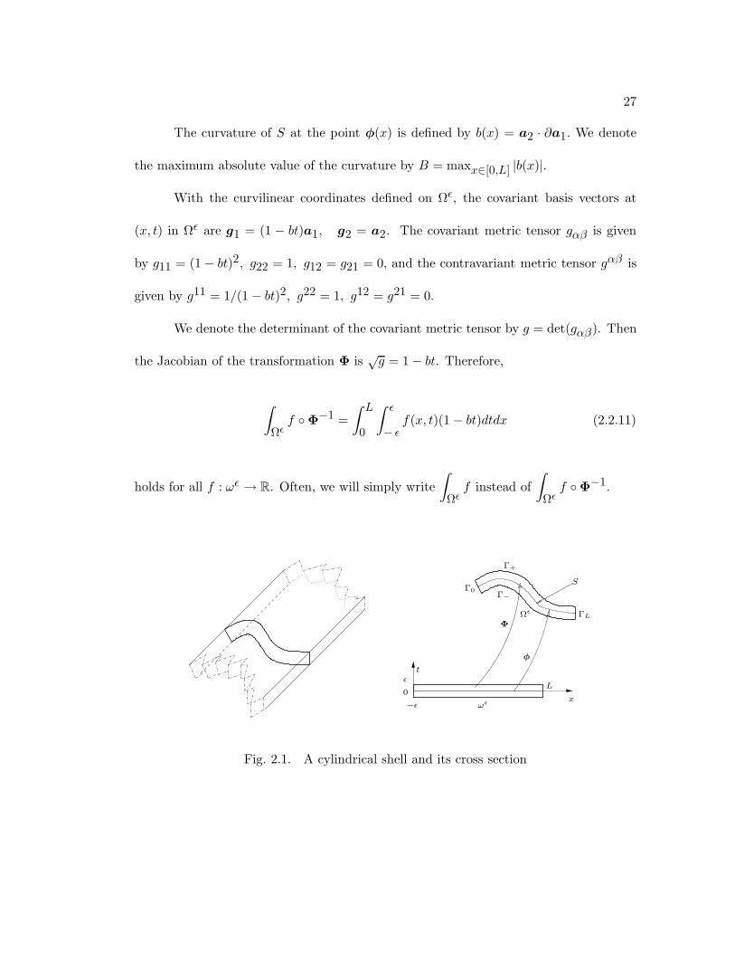
27

The curvature of S at the point φ(x) is defined by b(x) = a2 · ∂a1. We denote

the maximum absolute value of the curvature by B = maxx∈[0,L] |b(x)|.

With the curvilinear coordinates defined on Ωε, the covariant basis vectors at

(x, t) in Ωε are g1 = (1 − bt)a1, g2 = a2. The covariant metric tensor gαβ is given

by g11 = (1− bt)2, g22 = 1, g12 = g21 = 0, and the contravariant metric tensor gαβ is

given by g11 = 1/(1 − bt)2, g22 = 1, g12 = g21 = 0.

We denote the determinant of the covariant metric tensor by g = det(gαβ). Then

the Jacobian of the transformation Φ is√g = 1− bt. Therefore,

∫Ωεf Φ−1 =

∫ L

0

∫ ε

− εf(x, t)(1− bt)dtdx (2.2.11)

holds for all f : ωε → R. Often, we will simply write∫

Ωεf instead of

∫Ωεf Φ−1.

ωεx

Φ

t

0L

−ε

ε

S

Γ+

Γ−

ΓL

φ

Ωε

Γ0

Fig. 2.1. A cylindrical shell and its cross section

28

The Christoffel symbols of this metric are

Γ∗111 =−∂bt1− bt , Γ∗112 =

−b1− bt , Γ∗122 = 0,

Γ∗211 = b(1− bt), Γ∗212 = 0, Γ∗222 = 0.

The geometric equation becomes

χ11(v∼) = ∂v1 +∂bt

1− btv1 − b(1− bt)v2, χ22(v∼) = ∂tv2,

χ12(v∼) = χ21(v∼) =12

(∂tv1 + ∂v2) +b

1− btv1.

(2.2.12)

The row divergence of a tensor field σαβ , by (2.2.3), has the expression

σ1β‖β = ∂σ11 + ∂tσ12 − 2

∂bt

1− btσ11 − 3

b

1− btσ12,

σ2β‖β = ∂σ12 + ∂tσ22 + b(1− bt)σ11 − ∂bt

1− btσ12 − b

1− btσ22.

(2.2.13)

Let the surface force densities on Γ± be p∼± = pα±gα, the body force density be

q∼ = qαgα. The equilibrium equation is

σαβ‖β + qα = 0. (2.2.14)

The traction boundary conditions on Γ± expressed in terms of the contravariant com-

ponents of a stress field σ∼∼ read

σ12( · , ε) = p1+, σ12( · ,− ε) = −p1

−, σ22( · , ε) = p2+, σ22( · ,− ε) = −p2

−. (2.2.15)

29

According to the definition, a stress field σ∼∼ is statically admissible if both the

equations (2.2.14) and (2.2.15) are satisfied by its contravariant components.

The clamping boundary condition imposed on an admissible displacement field

v∼(x, t) is simply

v1(0, · ) = v1(L, · ) = v2(0, · ) = v2(L, · ) = 0. (2.2.16)

2.2.4 Rescaled stress and displacement components

To simplify the calculation, we introduce the rescaled components σαβ for a stress

tensor σαβ by

σ11 = (1− bt)2σ11, σ12 = (1− bt)σ12, σ22 = (1− bt)σ22. (2.2.17)

Then

σ1β‖β =1

(1− bt)2[∂σ11 + (1− bt)∂tσ12 − 2bσ12],

σ2β‖β =1

1− bt [∂σ12 + ∂tσ

22 + bσ11],

(2.2.18)

which is noticeably simpler than (2.2.13).

In these curvilinear coordinates, and in terms of the rescaled stress components,

the constitutive equation

χαβ = Aαβλγσλγ

30

takes the form

χ11 =2µ+ λ

4µ(µ + λ)(1− bt)2σ11 − λ

4µ(µ + λ)(1− bt)σ22,

χ12 = χ21 =1

2µ(1− bt)σ12,

χ22 =2µ + λ

4µ(µ+ λ)1

1− bt σ22 − λ

4µ(µ + λ)σ11.

(2.2.19)

For consistency with the rescaled stress components, we introduce the rescaled

components qα for the body force density and rescaled components pα for the surface

force density.

For the body force density, we define the rescaled components by

q∼ = qαgα = qα1

1− btaα. (2.2.20)

In components, we have q1 = (1− bt)2q1 and q2 = (1− bt)q2. The rescaled components

account the area change in the transverse direction of the cross section and more explicitly

reflect the variation of the body force density in that direction. We define the components

of the transverse average and moment of the body force density by

qαa =1

2 ε

∫ ε

− εq∼ · a

αdt, qαm =3

2 ε3

∫ ε

− εtq∼ · a

αdt. (2.2.21)

In the following, we assume the body force density changes linearly in t, or equivalently,

q∼ = (qαa + tqαm)aα. Under this assumption, the rescaled components are quadratic

31

polynomials in t, and we have qα = qα0 + tqα1 + t2qα2 , with qα0 = qαa , qα1 = qαm− bqαa , and

qα2 = −bqαm.

The ensuing calculations can be carried through if qα are arbitrary quadratic

polynomials in t. Without this restriction, we cannot apply the two energies principle

directly. For a general body force density, the convergence of the model can be proved

under some restriction on the transverse variation of the body force density. This issue

will be addressed in the general shell theory.

For the surface force density p∼±, we introduce the rescaled components pα± by

p∼+ = pα+gα = pα+1

1− b εgα, p∼− = pα−gα = pα−1

1 + b εgα. (2.2.22)

The rescaled components account the length differences of the upper and lower curves

of the shell cross section from middle curve. In terms of the rescaled surface force

components, we define

p1o =

p1+ − p1

−2

, p2o =

p2+ − p2

−2

, p1e =

p1+ + p1

−2 ε

, p2e =

p2+ + p2

−2 ε

, (2.2.23)

which are the odd and weighted even parts of the upper and lower surface forces.

In terms of the rescaled stress components σαβ and the rescaled applied force

components, the equilibrium equation (2.2.14) and the surface force condition (2.2.15)

can be written as

∂σ11 + (1− bt)∂tσ12 − 2bσ12 + q1 = 0,

∂σ12 + ∂tσ22 + bσ11 + q2 = 0

(2.2.24)

32

and

σ12( · ,± ε) = p1o ± ε p1

e, σ22( · ,± ε) = p2o ± ε p2

e. (2.2.25)

We introduce the rescaled displacement components vα for the displacement vec-

tor v∼ by expressing it as the combination of basis vectors on the middle curve, i.e.,

v∼ = vαgα = vαa

α, or equivalently, v1 = (1 − bt)v1, v2 = v2. In terms of the rescaled

components vα, by using (2.2.12), the geometric equation becomes

χ11(v∼) = (1− bt)(∂v1 − bv2), χ22(v∼) = ∂tv2,

χ12(v∼) = χ21(v∼) =12

[bv1 + ∂v2 + (1− bt)∂tv1].

(2.2.26)

And the clamping boundary condition is

vα(0, · ) = vα(L, · ) = 0. (2.2.27)

In summary, in terms of the rescaled components, the elasticity problem seeks dis-

placement components vα and stress components σαβ satisfying the constitutive equa-

tion (2.2.19), the equilibrium equation (2.2.24), the geometric equation (2.2.26) and the

boundary conditions (2.2.25) and (2.2.27).

2.3 The shell model

Our shell model is a 1D variational problem defined on the space H = [H10(0, L)]3.

The solution of the model is composed of three single variable functions that approx-

imately describe the shell displacement arising in response to the applied forces and

33

boundary conditions. For any (θ, u,w) ∈ H, we define

γ(u,w) = ∂u− bw, ρ(θ, u,w) = ∂θ + b(∂u− bw), τ(θ, u,w) = θ + ∂w + bu, (2.3.1)

which give the membrane strain, flexural strain and shear strain engendered by the

displacement functions (θ, u,w).

The model reads: Find (θε, uε, wε) ∈ H, such that

13ε2(2µ + λ?)

∫ L

0ρ(θε, uε, wε)ρ(φ, y, z)dx

+ (2µ + λ?)∫ L

0γ(uε,wε)γ(y, z)dx +

56µ

∫ L

0τ(θε, uε, wε)τ(φ, y, z)dx

= 〈f0 + ε2 f1, (φ, y, z)〉 ∀(φ, y, z) ∈ H, (2.3.2)

in which

λ? =2µλ

2µ + λ,

and the resultant loading functionals are given by

〈f0, (φ, y, z)〉 =56

∫ L

0p1oτ(φ, y, z)dx − λ

2µ + λ

∫ L

0p2oγ(y, z)

+∫ L

0[(p1e + q1

a − 2bp1o)y + (p2

e + q2a + ∂p1

o)z]dx (2.3.3)

and

〈f1, (φ, y, z)〉 = −13

∫ L

0[(bq1

a + 3bp1e − q1

m)φ+ bq1my + bq2

mz]dx

34

− λ

3(2µ + λ)

∫ L

0(p2e + bp2

o)ρ(φ, y, z)dx − 16

∫ L

0bp1eτ(φ, y, z)dx. (2.3.4)

The bilinear form in the left hand side of the variational formulation of the model

(2.3.2) is uniformly elliptic in the space H = [H10(0, L)]3. This conclusion follows from

the following theorem.

Theorem 2.3.1. The equivalency

‖ρ(θ, u,w)‖L2(0,L) + ‖γ(u,w)‖L2(0,L) + ‖τ(θ, u,w)‖L2(0,L) ' ‖(θ, u,w)‖H (2.3.5)

holds for all (θ, u,w) ∈ H = [H10(0, L)]3. Here ρ, γ and τ are the strain operators defined

in (2.3.1).

To prove this result, we need Peetre’s lemma.

Lemma 2.3.2. Let X, Y1, Y2 be Hilbert spaces, and let A1 : X → Y1 and A2 : X → Y2

be bounded linear operators with A1 injective and A2 compact. If there exists a constant

c > 0 such that

‖x‖X ≤ c(‖A1x‖Y1+ ‖A2x‖Y2

) ∀x ∈ X,

then there exists a constant c′ > 0 such that

‖x‖X ≤ c′‖A1x‖Y1∀x ∈ X.

For a proof of this lemma, see [28]. We give the proof of the theorem.

35

Proof of Theorem 2.3.1. The upper bound of the left hand side is obvious. For

the lower bound, we first see that

‖ρ(θ, u,w)‖L2(0,L) + (1 +B)‖γ(u,w)‖L2(0,L) + ‖τ(θ, u,w)‖L2(0,L)

≥ ‖∂θ‖L2(0,L) + ‖∂u− bw‖L2(0,L) + ‖∂w + θ + bu‖L2(0,L).

We consider the operators A1 and A2 from H to [L2(0, L)]3 defined by,

A1(θ, u,w) = (∂θ, ∂u− bw, ∂w+ θ+ bu), A2(θ, u,w) = (0, bw, θ+ bu), ∀ (θ, u,w) ∈ H.

The operator A1 is injective, since if (θ, u,w) ∈ kerA1, then θ = 0, ∂u − bw = 0 and

∂w+ bu = 0, so u∂u+w∂w = 0, therefore, u2 +w2 = constant. Since u and w vanish on

the end points of the interval, we must have u = w = 0. The operator A2 is obviously

compact. The statement follows from Lemma 2.3.2.

Theorem 2.3.1 shows that if the resultant loading functional f0 + ε2 f1 is in the dual

space of H, the model problem is uniquely solvable.

Remark 2.3.1. The requirement f0 + ε2 f1 ∈ H∗ can be met, if, say, the the applied

force functions are square integrable. To prove the convergence, we will need to assume

the tangential surface forces p1± ∈ H1(0, L). To prove the best possible convergence rate,

we will further need to assume the normal surface forces p2± ∈ H1(0, L). Henceforth, we

will assume that

pα± ∈ H1(0, L), qαa , qαm ∈ L2(0, L). (2.3.6)

36

This model is slightly different from that of Naghdi’s in the following aspects:

1. There is a shear correction factor 5/6. The best value for this factor is an

unresolved issue in shell theories. For the special case of plate, the value 5/6 is usually

accepted as the best. We will see that in the flexural case, the problem is not sensitive

to this value. In the case of membrane–shear, if this factor is changed, there must be a

corresponding change in the resultant loading functional, otherwise a poor choice of the

factor may lead to divergence of the model.

2. The expression for flexural strain is ∂θ + b(∂u − bw) while in the classical

Naghdi model it is ∂θ− b(∂u− bw). This change of the flexural strain operator rooted in

our derivation of the model, in which, the dimensionally reduced constitutive equation

was derived by roughly minimizing constitutive residual. Our choice leads to a smaller

constitutive residual. See Remark 2.4.1. Aother evidence favoring this change is provided

by modeling a semi-circular cylindrical shell, in which this change is simply a consequence

of more accurate integrations in the transverse direction in the process of classical Naghdi

model derivation.

3. The resultant loading functional contains more information than is normally

retained in the Naghdi model. The model convergence and convergence rate in the

relative energy norm can be proved if only f0 is kept in the loading functional. See

Section 7.1.

37

2.4 Reconstruction of the stress and displacement fields

From the model solution (θε, uε, wε) ∈ [H10(0, L)]3, we can rebuild a statically

admissible stress field by explicitly giving its contravariant components, and a kinemati-

cally admissible displacement field by giving its covariant components. We will prove the

convergence of both the reconstructed stress field and displacement field to the actual

fields determined from the 2D elasticity equations in the shell. The convergence will

be proved by using the two energies principle. To this end, we need to compute the

constitutive residual. We will see that the residual is formally small. Knowledge of the

behavior of the model solution will be necessary for a rigorous proof of the convergence.

2.4.1 Reconstruction of the statically admissible stress field

For brevity, we denote the flexural, membrane, and shear strains engendered by

the model solution by

ρε = ρ(θε, uε, wε), γε = γ(uε,wε), τ ε = τ(θε, uε, wε).

We define three single variable functions σ111 , σ11

0 , and σ120 by

σ111 = (2µ+ λ?)ρε +

λ

2µ + λ(p2e + bp2

o),

σ110 =

13b ε2 σ11

1 + (2µ + λ?)γε +λ

2µ + λp2o,

σ120 =

54µτε − 5

4p1o +

14bε2p1

e,

(2.4.1)

38

which furnish the principal part of the statically admissible stress field. It is straightfor-

ward to verify that these functions satisfy the following equations:

13ε2 ∂σ11

1 −23σ12

0 = ε2 bp1e +

13ε2(bq1

a − q1m),

∂σ110 −

23bσ12

0 = 2bp1o − p1

e − q1a +

13ε2 bq1

m,

bσ110 +

23∂σ12

0 = −p2e − ∂p1

o − q2a +

13ε2 bq2

m.

(2.4.2)

Actually, by substituting (2.4.1) into (2.4.2), we will get a system of three second order

ordinary differential equations, which is just the differential form of the variational model

equation (2.3.2). Obviously, the three principal stress functions are in L2(0, L). Further-

more, the equations in (2.4.2) clearly show that these three functions are in H1(0, L).

To complete the construction of a statically admissible stress field, we also need

three supplementary functions σ112 , σ22

0 , and σ221 . They are defined by

∂σ112 = −4bσ12

0 + ε2 bq1m,

σ220 =

12ε2(bσ11

1 + ∂p1e + q2

m − bq2a),

σ221 =

12ε(

23bσ11

2 + bσ110 + p2

e + ∂p1o + q2

a − ε2 bq2m).

(2.4.3)

Note that the first equation in (2.4.3) only gives ∂σ112 , so σ11

2 is determined up to an

arbitrary additive constant. We fix a particular solution by requiring∫ L

0σ11

2 = 0. Then

‖σ112 ‖H1(0,L) . B(‖σ12

0 ‖0 + ε2 ‖q1m‖0). (2.4.4)

39

With these six functions determined, the rescaled stress components σαβ then

are explicitly defined by

σ11 = σ110 + tσ11

1 + r(t)σ112 ,

σ12 = σ21 = p1o + tp1

e + q(t)σ120 ,

σ22 = p2o + tp2

e + q(t)σ220 + s(t)σ22

1 ,

(2.4.5)

where

r(t) =t2

ε2− 1

3, q(t) = 1− t2

ε2, s(t) =

t

ε(1− t2

ε2). (2.4.6)

Note that r is an even function of t and has zero integral over the interval [− ε, ε], and

q(± ε) = s(± ε) = 0. Following classical terminology, we will call σ110 the resultant

membrane stress, σ111 the first membrane stress moment, and σ11

2 the second membrane

stress moment. The function σ120 is responsible for the quadratic distribution of the

rescaled shear stress in the transverse direction and will be shown to be a higher order

term. The two functions σ220 and σ22

1 enrich the variation of the normal stress in the

transverse direction.

With this choice of the rescaled stress components, the surface traction condition

(2.2.25) is precisely satisfied. Combining the six equations in (2.4.2) and (2.4.3) and the

definition (2.4.5), we can verify that the equilibrium equation (2.2.24) is precisely satis-

fied. Therefore, by the relation between the rescaled components and the contravariant

components (2.2.17), we get the contravariant components σαβ of a statically admissible

40

stress field σ∼∼.

σ11 =1

(1− bt)2[σ11

0 + tσ111 + r(t)σ11

2 ],

σ12 = σ21 =1

1− bt [p1o + tp1

e + q(t)σ120 ],

σ22 =1

1− bt [p2o + tp2

e + q(t)σ220 + s(t)σ22

1 ].

(2.4.7)

2.4.2 Reconstruction of the kinematically admissible displacement field

The rescaled components of the displacement field are defined by

v1 = uε + tθε, v2 = wε + tw1 + t2w2. (2.4.8)

Here, w1 ∈ H10(0, L) and w2 ∈ H1

0(0, L) are two correction functions defined as solutions

of the following equations.

ε2(∂w1, ∂v)L2(0,L) + (w1, v)L2(0,L) = (1

2µ + λ?[p2o −

λ

2µ + λσ11

0 ], v)L2(0,L)

∀ v ∈ H10(0, L)

(2.4.9)

and

ε2(∂w2, ∂v)L2(0,L) + (w2, v)L2(0,L) = (1

2(2µ + λ?)[p2e −

λ

2µ + λσ11

1 ], v)L2(0,L)

∀ v ∈ H10(0, L).

(2.4.10)

The clamping boundary condition (2.2.27) is obviously satisfied. Note that this correc-

tion does not affect the middle curve displacement. So the basic pattern of the shell

41

deformation is already well captured by the model solution. The covariant components

of the kinematically admissible displacement field v∼ are

v1 = (1− bt)(uε + tθε), v2 = wε + tw1 + t2w2. (2.4.11)

These components are in H1(ωε), and satisfy the requirement of the two energies prin-

ciple.

2.4.3 Constitutive residual

We denote the residual of the constitutive equation by %αβ = Aαβλγσλγ −

χαβ(v∼), in which σαβ and vα are the components of the admissible stress and dis-

placement fields constructed from the model solution in the previous subsections.

By the formulae (2.2.26), we have

χ11(v∼) = (1− bt)(∂uε + t∂θε − bwε − btw1 − bt2w2)

= γε + tρε − 2btγε − b(1− bt)(tw1 + t2w2)− bt2∂θε,

χ12(v∼) = χ21(v∼) =12

(θε + ∂wε + buε + t∂w1 + t2∂w2) (2.4.12)

=12τε +

12

(t∂w1 + t2∂w2),

χ22(v∼) = w1 + 2tw2.

42

By the formulae (2.2.19), the definitions (2.4.1) and (2.4.5), and the identity (2µ +

λ)/[4µ(µ + λ)] = 1/(2µ + λ?), we have

A11λγσλγ = γε + tρε − 2btγε

+1

2µ+ λ?b2t2[σ11

0 + tσ111 + r(t)σ11

2 ] + [13b ε2(1− 2bt)− 2bt2]σ11

1

− λ

4µ(µ+ λ)(1− bt)[q(t)σ22

0 + s(t)σ221 ]− bt2p2

e

+1

2µ+ λ?(1− 2bt)r(t)σ11

2 , (2.4.13)

A12λγσλγ =

12µ

(1− bt)[p1o + tp1

e + q(t)σ120 ],

A22λγσλγ =

12µ+ λ?

(p2o −

λ

2µ+ λσ11

0 ) + t1

2µ+ λ?(p2e −

λ

2µ + λσ11

1 )

+1

2µ+ λ?q(t)σ22

0 + s(t)σ221 +

bt

1− bt [p2o + tp2

e + q(t)σ220 + s(t)σ22

1 ]

− λ

4µ(µ+ λ)r(t)σ11

2 .

Subtracting (2.4.12) from (2.4.13), we obtain the following expressions for the constitu-

tive residual:

%11 =1

2µ+ λ?b2t2[σ11

0 + tσ111 + r(t)σ11

2 ] + [13b ε2(1− 2bt)− 2bt2]σ11

1

− λ

4µ(µ+ λ)(1− bt)[q(t)σ22

0 + s(t)σ221 ]− bt2p2

e

+ b(1− bt)(tw1 + t2w2) + bt2∂θε

+1

2µ+ λ?(1− 2bt)r(t)σ11

2 , (2.4.14)

%12 =1

2µ[54q(t)− 1](µτε − p1

o)−12

(t∂w1 + t2∂w2)

43

+1

2µ[t+

14q(t)b ε2]p1

e −1

2µbt[p1

o + tp1e + q(t)σ12

0 ] (2.4.15)

%22 = [1

2µ+ λ?(p2o −

λ

2µ+ λσ11

0 )− w1] + t[1

2µ + λ?(p2e −

λ

2µ+ λσ11

1 )− 2w2]

+1

2µ+ λ?q(t)σ22

0 + s(t)σ221 +

bt

1− bt [p2o + tp2

e + q(t)σ220 + s(t)σ22

1 ]

− λ

4µ(µ+ λ)r(t)σ11

2 . (2.4.16)

Remark 2.4.1. If we had not made the sign change in the flexural strain ρ(θ, u,w)

discussed earlier, there would be an additional term 2btγ(uε,wε) in the residual %11.

Our variant does make the residual smaller, at least formally.

Formally, most of the terms in the above residual expressions contain a factor

of the form ε, t or smaller (recall that σ220 and σ22

1 have a small factor in their own

expressions (2.4.3)). In the expression of %11, the only term not formally small is the

last one, whose magnitude is determined by that of σ112 . The big term in the expression

of %12 is in the first one, which is determined by

µτε − p1o. (2.4.17)

This term is also the dominant part in the expression of σ120 , see (2.4.1). We will prove

that µτε − p1o is indeed small. Therefore, σ12

0 is small, and by (2.4.4), so is σ112 .

The definitions (2.4.9) and (2.4.10) of the correction functions w1 and w2 were

made to minimize the first two terms in the expression of %22, at the same time, they

44

minimize the two terms t∂w1 and t2∂w2 in the expression of %12. Therefore, we shall

be able to show that %22 is small as well.

2.5 Justification

The formal observations we made in the previous section do not furnish a rigorous

justification, since the applied forces and the model solution may depend on the the shell

thickness. To prove the convergence, we need to make some assumptions on the applied

loads, and get a good grasp of the behavior of the model solution when the shell thickness

tends to zero. Since we wish to bound the relative error, in addition to the upper bound

that can be determined from the constitutive residual, we need to have a lower bound

on the model solution.

2.5.1 Assumption on the applied forces

Henceforth, we assume that all the applied force functions explicitly involved in

the resultant loading functional of the model are independent of ε, i.e., the single variable

functions

pαo , pαe , q

αa , and qαm are independent of ε. (2.5.1)

This assumption is different from the usual assumption adopted in asymptotic theories,

according to which, the functions ε−1 pαo , rather than pαo themselves, should have been

assumed to be independent of ε. Our assumption on pαe , qαa and qαm is the same as the

usual one. This different assumption will reveal the potential advantages of the Naghdi-

type model over the Koiter-type model. The convergence theorem can also be proved

45

under the usual assumption on the applied forces, but it can be proved that the difference

between the two types of models then is negligible.

2.5.2 An abstract theory

Under the assumption (2.5.1) on the applied forces, the model (2.3.2) is an ε-

dependent variational problem fitting into the abstract problem that we shall discuss

in Chapter 3, cf., (3.2.2). The following convergence bounds (2.5.4) and (2.5.7) easily

follow from Theorem 3.3.1.

Let U, V , and H be Hilbert spaces, A : H → U a bounded linear operator, and

B : H → V a bounded linear continuous surjection. We assume that

‖Au‖U + ‖Bu‖V ' ‖u‖H ∀ u ∈ H. (2.5.2)

For any f0, f1 ∈ H∗ and f0 6= 0, we consider the variational problem

ε2(Au,Av)U + (Bu,Bv)V = 〈f0 + ε2 f1, v〉,

u ∈ H, ∀v ∈ H.

(2.5.3)

It is obvious that under the equivalency assumption (2.5.2), this variational problem has

a unique solution uε ∈ H that is dependent on ε. When ε → 0, the behavior of the

solution uε is drastically different depending on whether f0|kerB is nonzero or not. As

we shall see, in the former case, the solution uε blows up at the rate of O(ε−2), while in

the latter case uε tends to a finite limit.

46

For the first case, to get more accurate description of the behavior of the solu-

tion, we rescale the problem by assuming f0 = ε2 F0 and f1 = ε2 F1 with F0, F1 ∈ H

independent of ε. Under this assumption, we have the convergence estimate

‖Auε −Au0‖U + ε−1 ‖Buε‖V . ε ‖F0‖H∗ + ε2 ‖F1‖H∗ , (2.5.4)

in which u0 ∈ kerB is independent of ε and is the solution of the limit problem

(Au0, Av)U = 〈F0, v〉 ∀ v ∈ kerB. (2.5.5)

Since F0|kerB 6= 0, we must have Au0 6= 0.

For the second case, since f0 ∈ (kerB)a (the annihilator of kerB) and B is

surjective, there exists a unique ζ0 ∈ V , such that

〈f0, v〉 = (ζ0, Bv)V ∀ v ∈ H. (2.5.6)

In this case, there exists a unique u0 ∈ H such that Bu0 = ζ0, and we have the

convergence estimate

‖Auε −Au0‖U + ε−1 ‖Buε − ζ0‖V . ε(‖f0‖H∗ + ‖f1‖H∗). (2.5.7)

It can be shown that the limit u0 can be determined as u0 = u00 + u0

1. Here

(Au00, Av)U + (Bu0

0, Bv)V = 0 ∀v ∈ kerB, i.e., u00 is in the orthogonal complement of

kerB in H with respect to the inner product (A · , A · )U + (B · , B · )V that, due to the

47

equivalency assumption (2.5.2), is equivalent to the original inner product of H. And

u01 ∈ kerB is the solution of the limit problem corresponding to f1,

(Au01, Av)U = 〈f1, v〉 ∀ v ∈ kerB. (2.5.8)

Since f0 6= 0, we have ζ0 6= 0.

2.5.3 Asymptotic behavior of the model solution

To fit the model problem (2.3.2) in the abstract framework (2.5.3), we introduce

the following Hilbert spaces,

H = [H10(0, L)]3, U = L2(0, L), V = [L2(0, L)]2.

The inner product in H is the usual one. The inner products in U and V will be changed

slightly and equivalently. For ρ1, ρ2 ∈ U , we define

(ρ1, ρ2)U =13

(2µ+ λ?)(ρ1, ρ2)L2(0,L)

and for [γ1, τ1], [γ2, τ2] ∈ V , we define

([γ1, τ1], [γ2, τ2])V = (2µ + λ?)(γ1, γ2)L2(0,L) +56µ(τ1, τ2)L2(0,L).

We define the operators by

A(θ, u,w) = ρ(θ, u,w) ∀ (θ, u,w) ∈ H,

48

which is just the flexural strain operator, and

B(θ, u,w) = [γ(u,w), τ(θ, u,w)] ∀ (θ, u,w) ∈ H,

which combines the membrane and shear strains engendered by the displacement func-

tions.

The equivalence (2.3.5) that was established in Theorem 2.3.1 guaranteed the

condition (2.5.2). To use the abstract results, we also need to show that the operator B

is surjective. To this end, it is convenient to consider the dual operator B∗ of B. It is

easy to see that

B∗ : [L2(0, L]2 −→ [H−1(0, L)]3,

B∗(ζ, η) = (η, bη − ∂ζ,−∂η − bζ) ∀ (ζ, η) ∈ [L2(0, L]2.

We have

Lemma 2.5.1. If the curvature b of the middle curve S of the cross section of the cylin-

drical shell is not identically equal to zero, then the dual operator B∗ is injective and has

closed range.

Proof. If (ζ, η) ∈ kerB∗, then

‖η‖−1 = 0, ‖bη − ∂ζ‖−1 = 0, and ‖∂η + bζ‖−1 = 0,

49

so we have

η = 0, and ‖∂ζ‖−1 = 0, ‖bζ‖−1 = 0.

Since the curvature b is not identically equal to zero, we must have ζ = 0.

By viewing B∗ as the operator A1 in Lemma 2.3.2, and considering the compact

operator

A2 : [L2(0, L)]2 −→ [H−1(0, L)]3

defined by A2(η, ζ) = (0, bη, bζ), the desired result will follow from lemma 2.3.2.

The statement that the operator B is surjective then follows from the closed range

theorem.

Remark 2.5.1. If the curvature b is identically equal to zero, the operator B is still

surjective, but the range will be [L2(0, L)/R] × L2(0, L). All the results of this section

still apply.

In accordance with the abstract theory, when the shell thickness tends to zero,

the behavior of the model solution (θε, uε, wε) can be dramatically different for whether

f0|kerB 6= 0 (2.5.9)

or

f0|kerB = 0. (2.5.10)

50

We assume f0 6= 0, otherwise, the model is reduced down to a problem loaded by ε2 f1,

and all the analysis can be likewisely carried out and the convergence theorem in the

relative energy norm can also be proved.

a. Undeformed b. Flexural deformation

c. Membrane deformation d. Shear deformation

Fig. 2.2. Deformations of a cylindrical shell

Since the geometry of the middle surface of a cylindrical shell and the two sides

clamping boundary condition together do not inhibit pure flexural deformation (kerB 6=

0), a plane strain cylindrical shell problem can be classified as a flexural shell. However

the behavior of the shell is very different depending on whether or not the applied forces

make the pure flexural deformation happen. Similar situations for the second case arise

in stretching a plate, or twisting a plate by tangential surface forces that are equal in

magnitude but opposite in direction on the upper and lower surfaces. If the applied

forces do bring about the non-inhibited asymptotically pure flexural deformation, see

Figure 2.2 (b), the flexural energy will dominate membrane and shear strain energies.

51

If the applied force does not make the pure flexural deformation happen, as shown by

Figure 2.2 (c) (d), the membrane and shear strain energies together will dominate the

flexural energy. Since their magnitudes might be the same, there is no way for us to

distinguish the membrane and shear energies. For this reason, and for consistency with

terminologies in general shell theory, we call the first case the case of flexural shells, and

the second one the membrane–shear shells.

For a flexural shell, the solution blows up at the rate of O(ε−2). To get an

accurate grasp of the model solution behavior, we need to scale the loading functional

as we did for the abstract problem. This scaling is equivalently imposed on the applied

force functions by assuming

pαo = ε2 Pαo , pαe = ε2 Pαe , qαa = ε2Qαa , qαm = ε2Qαm, (2.5.11)

with Pαo , Pαe ,Qαa ,Qαm single variable functions independent of ε. The resultant loading

functionals are accordingly scaled as f0 = ε2 F 0, f1 = ε2 F 1, with F 0 and F 1

independent of ε. The expressions for F 0 and F 1 are the same as (2.3.3) and (2.3.4),

had the lower case letters been replaced by capital letters. By the estimate (2.5.4) we

have

‖ρε − ρ0‖L2(0,L) + ε−1 ‖γε‖L2(0,L) + ε−1 ‖τε‖L2(0,L) . ε, (2.5.12)

52

in which ρ0 = ρ(θ0, u0, w0), and (θ0, u0, w0) ∈ kerB is the solution of the limit problem

13

(2µ + λ?)∫ L

0ρ(θ0, u0, w0)ρ(φ, y, z)dx = 〈F 0, (φ, y, z)〉 ∀ (φ, y, z) ∈ kerB,

(θ0, u0, w0) ∈ kerB.

(2.5.13)

This limit problem is nothing else but the limit flexural shell model. Since F 0|kerB 6= 0,

we have ρ0 6= 0.

For a membrane–shear shell, when ε→ 0, the model solution (θε, uε, wε) converges

to a finite limit. In this case, the resultant loading functional can be reformulated as

〈f0, (φ, y, z)〉 = (ζ0, B(φ, y, z))V ∀ (φ, y, z) ∈ H.

Note that if the curvature b is not identically equal to zero, the strain operator γ(u,w) =

∂u− bw is surjective from [H10(0, L)]2 to L2(0, L). Recalling the expression (2.3.3):

〈f0, (φ, y, z)〉 =56

∫ L

0p1oτ(φ, y, z)dx − λ

2µ + λ

∫ L

0p2oγ(y, z)

+∫ L

0[(p1e + q1

a − 2bp1o)y + (p2

e + q2a + ∂p1

o)z]dx,

we see that the condition f0|kerB = 0 is equivalent to that the bounded linear functional

defined by the second term in the right hand side of this equation vanishes on the kernel of

the strain operator γ. Therefore, by the closed range theorem, the condition f0|kerB = 0

53

is equivalent to the unique existence of γ0 ∈ L2(0, L), such that

〈f0, (φ, y, z)〉 = (2µ + λ?)∫ L

0γ0γ(y, z)dx +

56µ

∫ L

0

1µp1oτ(φ, y, z)dx ∀ (φ, y, z) ∈ H.

Recalling the definition of inner product in the space V , it is readily seen that the

element ζ0 ∈ V in the abstract theory takes the form

ζ0 = (γ0,1µp1o).

By the estimate (2.5.7), we get

‖ρε − ρ0‖L2(0,1) + ε−1 ‖γε − γ0‖L2(0,L) + ε−1 ‖τε − 1µp1o‖L2(0,L) . ε, (2.5.14)

in which ρ0 = ρ(θ0, u0, w0) with (θ0, u0, w0) ∈ H be the limit of the solution (θε, uε, wε).

Actually, we also have γ0 = γ(θ0, u0, w0) and1µp1o = τ(θ0, u0, w0).

By their definitions (2.4.9), (2.4.10), and Theorem 3.3.6 of Chapter 3, we have

the following estimates on the correction functions w1 and w2.

ε ‖∂w1‖L2(0,L) + ‖ 12µ + λ?

(p2o −

λ

2µ + λσ11

0 )− w1‖L2(0,L)

. ε1/2[‖p2o‖H1(0,L) + ‖σ11

0 ‖H1(0,L)] (2.5.15)

54

and

ε ‖∂w2‖L2(0,L) + ‖ 12µ + λ?

(p2e −

λ

2µ + λσ11

1 )− 2w2‖L2(0,L)

. ε1/2[‖p2e‖H1(0,L) + ‖σ11

1 ‖H1(0,L)]. (2.5.16)

2.5.4 Convergence theorem

With all the above preparations, we are ready to prove the convergence theorem.

We denote the energy norm of a stress field σ∼∼ and a strain field χ∼∼ defined on the shell

cross section Ωε by

‖σ∼∼‖Eε = (∫

ΩεAαβλγσ

λγσαβ)1/2 and ‖χ∼∼‖Eε = (∫

ΩεCαβλγχλγχαβ)1/2,

respectively. Since the elasticity tensor Cαβλγ and the compliance tensor Aαβλγ are

uniformly positive definite and bounded, the energy norms are equivalent to the sums of

the L2(ωε) norms of the tensor components.

Theorem 2.5.2. Assume that the surface force functions have the regularity pα± ∈

H1(0, L) and the body force functions qαa , qαm ∈ L2(0, L). Let σ∼∼

∗ be the actual stress

distribution over the loaded shell, and v∼∗ the true displacement field arising in response

to the applied forces and boundary conditions. Based on the model solution (θε, uε, wε),

we define the statically admissible stress field σ∼∼ by the formulae (2.4.7), and define the

kinematically admissible displacement field v∼ by the formulae (2.4.11). We have the

55

estimate‖σ∼∼∗ − σ∼∼‖Eε + ‖χ∼∼(v∼

∗)− χ∼∼(v∼)‖Eε‖χ∼∼(v∼)‖Eε

. ε1/2 . (2.5.17)

Proof. The proof is based on the two energies principle, the formulae for the constitutive

residual (2.4.14) – (2.4.16), the asymptotic behaviors (2.5.12) and (2.5.14) of the model

solution, and the estimates (2.5.15) and (2.5.16) on the correction functions. Since the

behaviors of the model solution are very different for flexural shells and membrane–shear

shells, we prove the theorem for the two cases separately. In the following, we will simply

denote the norm ‖ · ‖L2(ωε) by ‖ · ‖.

Flexural shells

This is the case in which the solution blows up at the rate of O(ε−2). To

ease the analysis, we scale the loading functions by assuming that (2.5.11) holds, with

Pαo , Pαe ,Q

αa ,Q

αm single variable functions independent of ε. Note that, since we are con-

sidering the relative error estimate, this scaling is not a real restriction on the applied

force functions. With this scaling, we have the estimate (2.5.12), from which, we get

‖ρε − ρ0‖L2(0,L) . ε, ‖γε‖L2(0,L) . ε2, ‖τε‖L2(0,L) . ε

2 . (2.5.18)

From the equivalence (2.3.5), we get

‖θε‖H1(0,L) + ‖uε‖H1(0,L) + ‖wε‖H1(0,L) ' 1 ' ‖ρ0‖L2(0,L). (2.5.19)

56

By the definition (2.4.1), we have

σ110 =

13b ε2 σ11

1 + (2µ + λ?)γε +λ

2µ + λε2 P 2

o ,

σ111 = (2µ + λ?)ρε +

λ

2µ + λε2(P 2

e + bP 2o ),

σ120 =

54µτε − 5

4ε2 P 1

o +14bε4P 1

e ,

(2.5.20)

from which, we have the estimates

‖σ110 ‖L2(0,L) . ε

2, ‖σ111 ‖L2(0,L) ' 1, ‖σ12

0 ‖L2(0,L) . ε2 . (2.5.21)

By the estimate (2.4.4), we have

‖σ112 ‖H1(0,L) . ε

2 . (2.5.22)

From the first and last equations of (2.4.2), we see the estimates

‖σ110 ‖H1(0,L) . ε

2, ‖σ111 ‖H1(0,L) ' 1. (2.5.23)

From the last two equations in (2.4.3), we see the estimates

‖σ220 ‖L2(0,L) . ε

2, ‖σ221 ‖L2(0,L) . ε

3 . (2.5.24)

57

By the estimates on the correction functions (2.5.15) and (2.5.16), we have

ε ‖∂w1‖L2(0,L) + ‖ 12µ + λ?

(ε2 P 2o −

λ

2µ+ λσ11

0 )− w1‖L2(0,L) . ε5/2,

ε ‖∂w2‖L2(0,L) + ‖ 12µ + λ?

(ε2 P 2e −

λ

2µ + λσ11

1 )− 2w2‖L2(0,L) . ε1/2 .

(2.5.25)

From the equation (2.4.12), we see that in the expression of χ11(v∼), the term

tρ(θε, uε, wε) dominates in L2(ωε), and by (2.5.18), we get the lower bound ‖χ11(v∼)‖2 &

ε3, and so

‖χ∼∼(v∼)‖2Eε & ε3 . (2.5.26)

By the two energies principle, we have

‖σ∼∼∗ − σ∼∼‖

2Eε + ‖χ∼∼(v∼

∗)− χ∼∼(v∼)‖2Eε =∫

ΩεCαβλγ%λγ%αβ

. ‖%11‖2 + ‖%12‖2 + ‖%22‖2.

(2.5.27)

In the expression (2.4.14) of %11, we can see that the square integrals over ωε of all

the terms are bounded by O(ε5), therefore, we have ‖%11‖2 . ε5. From the expression

(2.4.15) of %12, we see that the square integrals of all the terms are bounded by O(ε4),

and so we have ‖%12‖2 . ε4. From the expression (2.4.16) of %22, we see the bounds are

O(ε4), and so ‖%22‖2 . ε4.

Therefore, by (2.5.27), we get the upper bound

‖σ∼∼∗ − σ∼∼‖

2Eε + ‖χ∼∼(v∼

∗)− χ∼∼(v∼)‖2Eε . ε4 (2.5.28)

58

The conclusion of the theorem for the case of flexural shells then follows from the lower

bound (2.5.26) and this upper bound.

Membrane–shear shells

In this case, under the assumption that pαo , pαe , qαa , and qαm are independent of ε,

the model solution (θε, uε, wε) converges to a finite limit in the space H when ε→ 0, so

we have

‖θε‖H1(0,L) + ‖uε‖H1(0,L) + ‖wε‖H1(0,L) . 1.

From the estimate (2.5.14), we get

‖ρε‖L2(0,L) . 1, ‖γε − γ0‖L2(0,L) . ε2, ‖µτε − p1

o‖L2(0,L) . ε2 . (2.5.29)

Since ζ0 6= 0, we know that γ0 and p1o can not be zero simultaneously. From the equation

(2.4.1) we see

‖σ110 ‖L2(0,L) . 1, ‖σ11

1 ‖L2(0,L) . 1, ‖σ120 ‖L2(0,L) . ε

2 . (2.5.30)

By the estimate (2.4.4), we have

‖σ112 ‖H1(0,L) . ε

2 . (2.5.31)

From the first and last two equations of (2.4.2), we see the estimates

‖σ110 ‖H1(0,L) . 1, ‖σ11

1 ‖H1(0,L) . 1. (2.5.32)

59

From the last two equations in (2.4.3), we see the estimates

‖σ220 ‖L2(0,L) . ε

2, ‖σ221 ‖L2(0,L) . ε . (2.5.33)

By the estimates on the correction functions (2.5.15) and (2.5.16), we have

ε ‖∂w1‖L2(0,L) + ‖ 12µ + λ?

(p2o −

λ

2µ + λσ11

0 )− w1‖L2(0,L) . ε1/2,

ε ‖∂w2‖L2(0,L) + ‖ 12µ+ λ?

(p2e −

λ

2µ+ λσ11

1 )− 2w2‖L2(0,L) . ε1/2 .

(2.5.34)

From the equation (2.4.12), we see that in the expression of χ11(v∼), the term γ(uε,wε)

dominates, and in the expression of χ12(v∼), the term12τ(θε, uε, wε) dominates. Asymp-

totically, we have the equivalency

‖γε‖L2(0,L) + ‖τε‖L2(0,L) ' ‖γ0‖L2(0,L) + ‖ 1

µp1o‖L2(0,L) ' 1. (2.5.35)

We get the lower bound ‖χ11(v∼)‖2 + ‖χ12(v∼)‖2 & ε, and so

‖χ∼∼(v∼)‖2Eε & ε . (2.5.36)

In the expression (2.4.14) of %11, we can see that the square integrals over ωε of all

the terms are bounded by O(ε3), therefore, we have ‖%11‖2 . ε3. From the expression

(2.4.15) of %12, we see all the terms are bounded by O(ε2), and so we have ‖%12‖2 . ε2.

From the expression (2.4.16) of %22, we see the bound is ‖%22‖2 . ε2.

60

By the two energies principle, we have

‖σ∼∼∗ − σ∼∼‖

2Eε + ‖χ∼∼(v∼

∗)− χ∼∼(v∼)‖2Eε . ‖%11‖2 + ‖%12‖2 + ‖%22‖2 . ε2 . (2.5.37)

The conclusion of the theorem for the case of membrane–shear shells then follows from

the lower bound (2.5.36) and this upper bound.

2.6 Shear dominated shell examples

To emphasize the necessity of using the Naghdi-type model in some cases, we give

two examples for which the model equations are explicitly solvable. For these problems,

the Koiter model and limiting flexural model only give solutions that are identically

equal to zero, while our Naghdi-type model can very well capture the shear dominated

deformations.

2.6.1 A beam problem

p∼−

p∼+

b. Shear dominated deformationa. Undeformed

Fig. 2.3. Shear dominated deformation of a beam

61

We consider a special plane strain cylindrical shell whose cross section is a thin

rectangle with thickness 2 ε and length L = 1. The curvature of the middle curve then

is b ≡ 0. The applied forces are: q∼ = 0, p∼± = ±a1. The leading term of the resultant

loading functional (2.3.3) is given by

〈f0, (φ, y, z)〉 =56

∫ 1

0τ(φ, y, z)dx.

The condition f0|kerB = 0 is obviously satisfied. Therefore the limiting flexural shell

model only gives a zero solution. So does Koiter’s model.

The model (2.3.2), written in differential form, reduces to

−13ε2(2µ + λ?)∂2θε +

56µ(θε + ∂wε) =

56,

−(2µ+ λ?)∂2uε = 0, −56µ∂(θε + ∂wε) = 0,

(θε, uε, wε) ∈ [H10(0, 1)]3,

(2.6.1)

which is just the Timoshenko beam bending and stretching model [3]. The solution is

given by

θε = cεx(1− x), uε = 0, wε = −13cε(x− 1

2)x(1− x),

where cε = [µ

6+

16 ε2 µ(µ+ λ)5(2µ + λ)

]−1. We see the convergences:

limε→0

θε =1µ

6x(1− x), limε→0

wε = −21µ

(x− 12

)x(1− x), limε→0

(θε + ∂wε) =1µ.

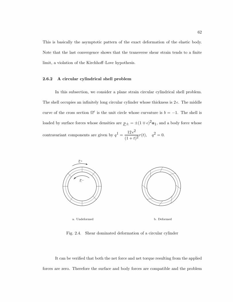
62

This is basically the asymptotic pattern of the exact deformation of the elastic body.

Note that the last convergence shows that the transverse shear strain tends to a finite

limit, a violation of the Kirchhoff–Love hypothesis.

2.6.2 A circular cylindrical shell problem

In this subsection, we consider a plane strain circular cylindrical shell problem.

The shell occupies an infinitely long circular cylinder whose thickness is 2 ε. The middle

curve of the cross section Ωε is the unit circle whose curvature is b = −1. The shell is

loaded by surface forces whose densities are p∼± = ±(1∓ ε)2a1, and a body force whose

contravariant components are given by q1 =12 ε2

(1 + t)2r(t), q2 = 0.

p∼+

p∼−

b. Deformeda. Undeformed

Fig. 2.4. Shear dominated deformation of a circular cylinder

It can be verified that both the net force and net torque resulting from the applied

forces are zero. Therefore the surface and body forces are compatible and the problem

63

is well defined. By using the formulae (2.2.21) to compute qαa and qαm, the resultant

loading functional in the model can be computed. We have

〈f0 + ε2 f1, (φ, y, z)〉 =56

∫ 2π

0τ(φ, y, z)dx

+ ε2[12

∫ 2π

0τ(φ, y, z)dx + 2

∫ 2π

0ydx− 2

∫ 2π

0φdx] + ε4〈r, (φ, y, z)〉,

where r is a functional independent of ε. The higher order term O(ε4 r) is provably

negligible. With this higher order term cutoff, we will have f0|kerB = 0. The model

solution then is

uε = 0, wε = 0, θε =1µ− 9

5µε2,

which gives a displacement field that is purely rotational. The covariant components

of the displacement field provided by this model are v1 = (1 + t)tθε, v2 = 0. The

covariant components of the strain tensor engendered by this displacement field are, by

the formulae (2.2.26),

χ11 = 0, χ22 = 0, χ12 =12θε =

12µ− 9

10µε2 . (2.6.2)

It can be easily checked that the stress field whose contravariant components are

given by

σ11 = 0, σ22 = 0, σ12 =1

1 + t[1− 2t + 3t2 − 2 ε2] (2.6.3)

64

is statically admissible. By using the formulae (2.2.19), we see that for the admissible

stress field defined by (2.6.3),

A11λγσλγ = A22λγσ

λγ = 0, A12λγσλγ =

12µ

(1 + t)[1− 2t + 3t2 − 2 ε2].

Therefore, the the constitutive residual can be bounded by

%11 = 0, %22 = 0, |%12| . ε .

From the two energies principle, we know that the pure rotational displacement given

by the model is very close to the exact displacement of this circular cylinder arising in

response to the applied forces. The error in the relative energy norm is O(ε). The shear

strain and stress absolutely dominate all the other strain and stress components. For

this problem, the Koiter model and the limiting flexural shell model only give a solution

that is identically equal to zero. This is a case for which the Naghdi-type model is

indispensable.

65

Chapter 3

Analysis of the parameter dependent

variational problems

3.1 Introduction

The plane strain cylindrical shell model (2.3.2) that we justified in the last chapter

can be put in the form of the abstract ε-dependent variational problem (3.2.2) below, and

Theorem 3.3.1 was essential to the justification. This abstract problem also applies to

the spherical shell model and general shell model that we are going to derive and justify.

It is the purpose of this chapter to establish all the a priori estimates that are necessary

for our analyses. The behavior of the solution of such ε-dependent can be drastically

different in different circumstances. We will classify the problem on the abstract level at

the end of this chapter. Results that will be used to analyze the relations between our

model and other existing shell theories will also be given.

3.2 The parameter dependent problem and its mixed formulation

For a Hilbert space X, we denote its dual by X∗, and for any f ∈ X∗, we use

iXf ∈ X to denote its Riesz representation. The isomorphism πX : X → X∗ is defined

as the inverse of iX , and is equal to iX∗ under the usual identification of X and X∗∗.

66

Let H, U , and V be Hilbert spaces, A and B be linear continuous operators

from H to U and V , respectively. We assume

‖Au‖2U + ‖Bu‖2V ' ‖u‖2H ∀ u ∈ H. (3.2.1)

By properly defining spaces and operators, the shell models we derive can be

written in the form of the ε-dependent variational problem:

ε2(Au,Av)U + (Bu,Bv)V = 〈f0 + ε2 f1, v〉,

u ∈ H, ∀ v ∈ H,

(3.2.2)

where f0, f1 ∈ H∗ are two functionals independent of ε, and f0 6= 0. It turns out that,

in all the cases we are going to analyze, when ε→ 0, the asymptotic behavior of solution

of this variational problem is mostly determined by the leading term f0. For this reason,

we first analyze the abstract problem

ε2(Au,Av)U + (Bu,Bv)V = 〈f, v〉,

u ∈ H, ∀ v ∈ H,

(3.2.3)

with f ∈ H∗ independent of ε. The behavior of the solution of (3.2.2) will be obtained

by a simple argument once the simpler problem (3.2.3) is fully understood.

The variational problem (3.2.3) represents the Timoshenko beam bending model

and Reissner–Mindlin plate bending model, with u standing for the transverse deflection

of the middle surface and rotation of normal fibers, and Au the bending strain and Bu

67

the transverse shear strain engendered by u. The Koiter shell model, which adopts the

Kirchhoff–Love assumption and so ignores the transverse shear deformation, takes this

form, with the variable u representing the middle surface displacement, Au the flexural

strain, and Bu the membrane strain. The Naghdi shell model, and the variant we derive,

can be put in this form if we let u be the middle surface displacement and normal fiber

rotation. The operator A defines the flexural strain and B combines the transverse

shear and membrane strains engendered by u. The spaces H is a multiple L2-based first

order Sobolev space, and U and V are equivalent to L2 or products of L2. Referring to

the physical background of the abstract problem, we will call ε2(Au,Au)U the flexural

energy, and (Bu,Bu)V the membrane–shear energy engendered by the displacement

function u.

Under the assumption (3.2.1), for any f ∈ H∗, the variational problem (3.2.3) has

a unique solution depending on ε. In what follows, whenever the ε dependence needs to

be emphasized, the solution will be denoted by uε. We are concerned with the behavior

of the solution of such problems, especially when ε is small.

If we set F = ε−2 f , the following rough estimate is obvious

‖uε‖H . ‖F‖H∗ . (3.2.4)

We will derive more accurate estimates on the solution of (3.2.3) by introducing

a mixed formulation. In what follows, we will need some basic results.

68

First we recall that if X and Y are Hilbert spaces with X ⊂ Y , and if X is dense

in Y , then the restriction operator defines an injection of Y ∗ onto a dense subspace of

X∗ (and we usually identify Y ∗ with that dense subspace).

We next recall the sum and intersection constructions for Hilbert spaces. If Hilbert

spaces X and Y are both continuously included in a larger Hilbert space, then the

intersection X ∩ Y and the sum X + Y are themselves Hilbert spaces with the norms

‖z‖X∩Y = (‖z‖2X + ‖z‖2Y )1/2 and ‖z‖X+Y = infz=x+y

(‖x‖2X + ‖y‖2Y )1/2,

and we have

Lemma 3.2.1. If in addition, X ∩Y is dense in both X and Y , then the dual spaces X∗

and Y ∗ can be viewed as subspace of (X ∩ Y )∗ and we have

X∗ + Y ∗ = (X ∩ Y )∗.

The operator B : H → V may have closed range in some problems, as in the cases

of Timoshenko beam bending model, the plain strain cylindrical shell model of Chapter 2

and other 1D models. This operator may have a range that is not closed in V , as in the

Reissner–Mindlin plate, Koiter and Naghdi shell models, as well as numerous singular

perturbation problems.

Let W = B(H) ⊂ V be the range of B, whose norm is defined by, for any ζ ∈W ,

‖ζ‖W = infζ=Bu

‖u‖H. (3.2.5)

69

With this norm, W is a Hilbert space isomorphic to H/ kerB. This space plays a crucial

role in the following analysis. For the Reissner–Mindlin bending model of a totally

clamped plate, this space is H∼(rot). Without loss of generality we may assume that W

is dense in V , otherwise, we can just replace V by the closure of W in it.

Associated with a Hilbert space X and any positive number ς, we define the

Hilbert spaces ςX. As set, ςX equals to X, but the norm is defined by ‖x‖ςX = ς‖x‖X .

Since W is dense in V , so V ∗ and ε V ∗ are dense in W ∗. The dual space of

W ∗ ∩ ε V ∗ is, by Lemma 3.2.1, W + ε−1 V .

If uε solves (3.2.3) and ξε = ε−2 πV Buε ∈ V ∗, then (uε, ξε) solves the mixed

problem

(Au,Av)U + 〈ξ,Bv〉 = 〈F, v〉 ∀ v ∈ H,

〈η,Bu〉 − ε2(ξ, η)V ∗ = 0 ∀ η ∈ V ∗,

u ∈ H, ξ ∈ V ∗.

(3.2.6)

For this mixed problem, we have the following result

Theorem 3.2.2. The mixed problem (3.2.6) has a unique solution (uε, ξε) ∈ H × V ∗,

and the equivalence

‖uε‖H + ‖ξε‖W ∗∩ε V ∗ ' ‖F‖H∗ (3.2.7)

holds.

Proof. The pair (uε, ξε) solves (3.2.6) if and only if ξε = ε−2 πV Buε and uε solves (3.2.3),

so the existence and uniqueness are established. From (3.2.4) and the first equation, we

70

get

‖uε‖H + ‖ξε‖W ∗ . ‖F‖H∗ .

Taking v = uε in the first equation and η = ξε in the second equation, we get the bound

on ‖ξε‖ε V ∗ . From the first equation, we easily get that ‖F‖H∗ . ‖uε‖H + ‖ξε‖W ∗ .

This theorem shows that the right space for the auxiliary variable ξε is W ∗∩ε V ∗.

To analyze the asymptotic behavior of the solution uε, we also need to consider

the following general mixed problem.

(Au,Av)U + 〈ξ,Bv〉 = 〈F, v〉 ∀ v ∈ H,

〈η,Bu〉 − ε2(ξ, η)V ∗ = 〈I, η〉 ∀ η ∈ V ∗,

u ∈ H, ξ ∈ V ∗.

(3.2.8)

here, I ∈ V . For this general mixed problem we have

Theorem 3.2.3. The mixed problem (3.2.8) has a unique solution (uε, ξε) ∈ H × V ∗,

and the equivalence

‖uε‖H + ‖ξε‖W ∗∩ε V ∗ ' ‖F‖H∗ + ‖I‖W+ε−1 V (3.2.9)

holds.

71

Proof. Let ζ0∗ = πV I, then 〈I, η〉 = (ζ0∗ , η)V ∗ . The problem (3.2.8) can be reformulated

as

(Au,Av)U + 〈ξ + ε−2 ζ0∗ , Bv〉 = 〈F, v〉 + ε−2〈ζ0

∗ , Bv〉 ∀ v ∈ H,

〈η,Bu〉 − ε2(ξ + ε−2 ζ0∗ , η)V ∗ = 0 ∀ η ∈ V ∗,

u ∈ H, ξ ∈ V ∗.

(3.2.10)

This formulation is in the form of (3.2.6), therefore, we get the existence and uniqueness

of the solution from Theorem 3.2.2. In the following, C1–C5 are constants independent

of ε.

From the first equation of (3.2.8), we get

‖ξε‖W ∗ ≤ C1(‖F‖H∗ + ‖Auε‖U ). (3.2.11)

Taking v = uε and η = ξε in (3.2.8), and subtracting the second equation from the first

equation, we get

‖Auε‖2U + ε2 ‖ξε‖2V ∗ = 〈F, uε〉 − 〈I, ξε〉,

so we have

‖Auε‖2U + ε2 ‖ξε‖2V ∗ ≤ C2(‖F‖H∗‖uε‖H + ‖I‖W+ε−1 V ‖ξε‖W ∗∩ε V ∗). (3.2.12)

From the second equation of (3.2.8) and the bound ‖I‖V . ‖I‖W+ε−1 V , we get

‖Buε‖V ≤ C3(ε2 ‖ξε‖V ∗ + ‖I‖W+ε−1 V ). (3.2.13)

72

Combining (3.2.11), (3.2.12) and (3.2.13), we get

‖Auε‖2U + ‖Buε‖2V + ε2 ‖ξε‖2V ∗ ≤ C4(‖F‖H∗‖uε‖H + ‖I‖W+ε−1 V ‖Auε‖U

+‖I‖W+ε−1 V ‖ξε‖ε V ∗ + ‖I‖W+ε−1 V ‖F‖H∗ + ‖I‖2

W+ε−1 V).

(3.2.14)

By using Cauchy’s inequality and (3.2.1), we get

‖Auε‖2U + ‖Buε‖2V + ε2 ‖ξε‖2V ∗ ≤ C5(‖F‖2H∗ + ‖I‖2W+ε−1 V

). (3.2.15)

The upper bound of the left hand side in (3.2.9) follows from (3.2.11) and (3.2.15).

The other direction follows from the formulation (3.2.8) directly.

This result is an extension of an equivalence theorem established for the Reissner–

Mindlin plate bending model in [8].

3.3 Asymptotic behavior of the solution

When ε → 0, the behavior of the solution uε of (3.2.3) is dramatically different

depending on whether

f |kerB 6= 0, (3.3.1)

or

f |kerB = 0. (3.3.2)

The asymptotic behavior needs to be discussed separately for these two cases. In the

first case, the solution blows up at the rate of O(ε−2). To fix the situation, we scale the

73

problem by assuming that F = ε−2 f is independent of ε. With this scaling, the problem

(3.2.3) or equivalently (3.2.6) can be viewed as a penalization of the constrained problem

minu∈kerB

12

(Au,Au)U − 〈F, u〉. (3.3.3)

This constrained problem has a unique nonzero solution u0 ∈ kerB. This minimization

problem can also be written in mixed form as

(Au,Av)U + 〈ξ,Bv〉 = 〈F, v〉 ∀ v ∈ H,

〈η,Bu〉 = 0 ∀ η ∈W ∗, u ∈ H, ξ ∈W ∗.

(3.3.4)

This mixed problem has a unique solution (u0, ξ0) with u0 ∈ kerB and ξ0 ∈W ∗. And

we have the equivalence

‖u0‖H + ‖ξ0‖W ∗ ' ‖F‖H∗ . (3.3.5)

In the second case, the problem is essentially a singular perturbation problem.

We do not need to scale the problem. From the definition of W , we know that B is

surjective from H to W . By the closed range theorem in functional analysis, there exists

a unique ζ0∗ ∈W ∗ such that

〈f, v〉 = 〈ζ0∗ , Bv〉 ∀ v ∈ H. (3.3.6)

74

3.3.1 The case of surjective membrane–shear operator

We first discuss the simpler case in which the operator B : H → V is surjective.

An example of this case is the plane strain cylindrical shell problems discussed in the

last chapter. In this case, we have W = V , W ∗ = V ∗, and

Theorem 3.3.1. Let H, U and V be Hilbert spaces, the linear operators A : H → U

bounded, and B : H → V bounded and surjective. We assume the equivalence (3.2.1)

holds, so the variational problem (3.2.3) has a unique solution uε ∈ H.

If f |kerB 6= 0, we assume F = ε−2 f is independent of ε. Then

‖Auε −Au0‖U + ε−1 ‖Buε‖V . ε ‖ξ0‖V ∗ . ε ‖F‖H∗ , (3.3.7)

where (u0, ξ0) is the solution of the ε-independent problem (3.3.4), with u0 ∈ kerB,

ξ0 ∈ V ∗, and u0 6= 0.

If f |kerB = 0, there exists a nonzero element ζ0∗ ∈ V ∗, such that

〈f, v〉 = 〈ζ0∗ , Bv〉 = (ζ0, Bv)V ∀ v ∈ H.

Here ζ0 ∈ V is the Riesz representation of ζ0∗ . There exists a unique u0 ∈ H, satisfying

Bu0 = ζ0 together with the estimate

‖uε − u0‖H . ε2 ‖ζ0‖V . (3.3.8)

75

Moreover

ε−1 ‖Auε −Au0‖U + ε−1 ‖Buε − ζ0‖V . ε ‖ζ0‖V = ε ‖f‖H∗ . (3.3.9)

Proof. We prove (3.3.7) first. Under the assumption of W = V , the solutions of the

mixed problems (3.2.6) and (3.3.4) satisfy

(Auε,Av)U + 〈ξε,Bv〉 = 〈F, v〉 ∀ v ∈ H,

〈Buε, η〉 − ε2(ξε, η)V ∗ = 0 ∀ η ∈ V ∗

and

(Au0, Av)U + 〈ξ0, Bv〉 = 〈F, v〉 ∀ v ∈ H,

〈η,Bu0〉 = 0 ∀ η ∈ V ∗,

respectively. Subtracting the second equation from the first one, and taking v = uε−u0,

η = ξε − ξ0, we get

(Auε −Au0, Auε −Au0)U + ε2(ξε − ξ0, ξε − ξ0)V ∗ = − ε2(ξ0, ξε − ξ0)V ∗ .

By using Cauchy’s inequality, we get

‖Auε −Au0‖2U + ε2 ‖ξε − ξ0‖2V ∗ . ε2 ‖ξ0‖2V ∗ .

The estimate (3.3.7) then follows from the fact that ξε = ε−2 πV Buε.

76

Now we assume f |kerB = 0. The variational problem (3.2.3) can be written as

ε2[(Auε,Av)U + (Buε,Bv)V ] + (1− ε2)(Buε,Bv)V = 〈f, v〉 ∀ v ∈ H. (3.3.10)

By the equivalency assumption (3.2.1), the bilinear form

(u, v)H = (Au,Av)U + (Bu,Bv)V

defines an inner product on H, which is equivalent to the original inner product. With

this new inner product, the space H will be denoted by H. The condition f |kerB = 0

means that there exists a unique u0 ∈ (kerB)⊥, the orthogonal complement of kerB in

H, such that

〈f, v〉 = (Bu0, Bv)V ∀ v ∈ H, (3.3.11)

and the operator B defines an isomorphism between (kerB)⊥ and V .

From the equation (3.3.10), it is not hard to see that uε ∈ (kerB)⊥. Substituting

(3.3.11) into (3.3.10), and taking v = uε − u0, with a little algebra, we get

ε2(uε − u0, uε − u0)H + (1− ε2)(Buε −Bu0, Buε −Bu0)V

= ε2(Bu0, Buε −Bu0)V − ε2(u0, uε − u0)H.

(3.3.12)

77

Since uε and u0 both belong to (kerB)⊥, we have ‖u0‖H . ‖Bu0‖V and ‖uε− u0‖H .

‖Buε −Bu0‖V . Therefore, by using Cauchy’s inequality, from (3.3.12), we get

ε2(uε − u0, uε − u0)H + (1− ε2)(Buε −Bu0, Buε −Bu0)V . ε4 ‖Bu0‖2V . (3.3.13)

Therefore,

‖uε − u0‖H ' ‖Buε −Bu0‖V . ε2 ‖Bu0‖V = ε2 ‖ζ0‖V .

The estimate (3.3.9) is a consequence of the equivalence assumption (3.2.1).

To get the estimate (3.3.8), the assumption that the operator B has closed range

is crucial. Without this assumption, we can not expect the convergence of the sequence

uε in the space H. This is a usual phenomena in singular perturbation problems and

a big trouble for numerical analysis of the general membrane–shear shells. This result is

the infinite dimensional version of the so-called Cheshire lemma.

The condition that the operator B is surjective is only satisfied by some special

problems. This condition is not met by the Reissner–Mindlin plate bending model, nor

the Koiter or Naghdi shell models. It does not apply to the spherical shell model and

the general shell model we are going to derive and justify either.

If the range of B is not closed, the space W is a proper subspace of V , so is V ∗

of W ∗. If V ∗ is identified with V through the Riesz representation theorem, we have

the inclusions W ⊂ V ∼ V ∗ ⊂ W ∗. We will show that in the case of f |kerB 6= 0, the

asymptotic behavior of the solution uε is largely determined by the position of ξ0, the

Lagrange multiplier defined in (3.3.4), between V ∗ and W ∗. The closer ξ0 to V ∗, the

stronger the convergence. In the best case of ξ0 ∈ V ∗, a convergence rate of the form

78

(3.3.7) can be obtained. In the worst case, i.e., we only have ξ0 ∈ W ∗, we will prove a

convergence, but without convergence rate.

In the case of f |kerB = 0, we must require ζ0∗ , the equivalent representation of f

in W ∗ defined in (3.3.6), to be in the smaller space V ∗. Then, the asymptotic behavior

of uε is determined by the position of ζ0, the Riesz representation of ζ0∗ in the space V ,

between W and V .

3.3.2 The case of flexural domination

In this subsection, we discuss the case of f |kerB 6= 0 without the assumption that

B is surjective. In this case we need to rescale the problem by assuming that F = ε−2 f

is independent of ε. We have

Theorem 3.3.2. Let (uε, ξε) be the solution of (3.2.6), and (u0, ξ0) be the solution of

(3.3.4), then

‖Auε −Au0‖U + ε−1 ‖Buε‖V . ε ‖ξ0‖ε−1W ∗+V ∗ (3.3.14)

Proof. Subtracting (3.3.4) from (3.2.6), we get

(A(uε − u0), Av)U + 〈ξε − ξ0, Bv〉 = 0 ∀ v ∈ H,

〈B(uε − u0), η〉 − ε2(ξε, η)V ∗ = 0 ∀ η ∈ V ∗.

(3.3.15)

Taking v = uε − u0 and η = ξε, and writing the second equation as

〈B(uε − u0), ξε − ξ0〉+ 〈B(uε − u0), ξ0〉 − ε2(ξε, ξε)V ∗ = 0,

79

together with the first equation

(A(uε − u0), A(uε − u0))U + 〈ξε − ξ0, B(uε − u0)〉 = 0,

we get

(A(uε − u0), A(uε − u0))U + ε2(ξε, ξε)V ∗ = 〈B(uε − u0), ξ0〉. (3.3.16)

By the definition (3.2.5) of the norm of W , and the equivalence assumption (3.2.1), we

have

‖B(uε − u0)‖W . ‖A(uε − u0)‖U + ‖B(uε − u0)‖V ,

and so

‖B(uε − u0)‖εW . ε ‖A(uε − u0)‖U + ε ‖B(uε − u0)‖V .

Therefore, we have the estimate

|〈B(uε − u0), ξ0〉| . [ε ‖A(uε − u0)‖U + ‖B(uε − u0)‖V ]‖ξ0‖ε−1W ∗+V ∗ . (3.3.17)

Recalling that ξε = πV ε−2Buε and Bu0 = 0, combining (3.3.16) and (3.3.17)

and using Cauchy’s inequality, we obtain

‖A(uε − u0)‖2U + ε−2 ‖Buε‖2V . ε2 ‖ξ0‖2

ε−1W ∗+V ∗ .

80

The desired result then follows.

The K-functional on the Hilbert couple [W ∗, V ∗] is given by

K(ε, ξ0, [W ∗, V ∗]) = ε ‖ξ0‖ε−1W ∗+V ∗ ,

see [9]. According to the definition of interpolation spaces based on the K-functional,

|K(ε, ξ0, [W ∗, V ∗])| . Cθ,q εθ ‖ξ0‖[V ∗,W ∗]1−θ,q .

If ξ0 is further assumed to belong to the interpolation space [V ∗,W ∗]1−θ,q, for some

0 < θ < 1 and 1 ≤ q ≤ ∞, or 0 ≤ θ ≤ 1 and 1 < q <∞, we have

‖Auε −Au0‖U + ε−1 ‖Buε‖V . εθ ‖ξ0‖[V ∗,W ∗]1−θ,q . (3.3.18)

In particular, if

ξ0 ∈ V ∗, (3.3.19)

we can take θ = 1 and obtain the stronger result

‖Auε −Au0‖U + ε−1 ‖Buε‖V . ε ‖ξ0‖V ∗ . (3.3.20)

The estimate (3.3.20) is an extension of a convergence theorem of solution of

the Reissner–Mindlin plate bending model to that of the Kirchhoff–Love plate bending

model in [4].

81

We will prove that the convergence rate of our 2D shell model solution to the 3D

shell solution in the relative energy norm is crucially related to this “regularity index” θ

of the Lagrange multiplier ξ0.

The condition (3.3.19) can be verified for the Reissner–Mindlin plate bending

model, if the plate is totally clamped, and the plate boundary and loading function are

smooth enough so that the H3 regularity of the Kirchhoff–Love model solution holds,

see [8]. For partially clamped plates and arbitrary shells, this index needs to be carefully

evaluated.

If we know nothing more than the minimum regularity of the Lagrange multiplier

ξ0 ∈W ∗, then we must choose θ = 0. The estimate (3.3.18) does not provide any useful

information. The following theorem will be used to prove the convergence, but without

a convergence rate, of the flexural shell model.

Theorem 3.3.3. Let uε be the solution of (3.2.6) and u0 be the solution of (3.3.4). We

have the convergence result

limε→0

[‖A(uε − u0)‖U + ε−1 ‖Buε‖V ] = 0. (3.3.21)

Proof. Taking v = uε in the equation (3.2.3), we get

(Auε,Auε)U + ε−2(Buε,Buε)V = 〈F, uε〉.

82

From this equation we see that there exists a constant C independent of ε, such

that

‖uε‖H + ‖ ε−1Buε‖V ≤ C.

Since bounded sets in a Hilbert space are weakly compact, there exists a subsequence,

εn → 0, an element u ∈ H, and an element p ∈ V , such that

uεn u in H, ε−1n Buεn p in V.

Since Buεn Bu in V , and Buεn → 0 in V , we have Bu = 0, so u ∈ kerB. Note that

we also have Auεn Au, so we have

(Au,Av)U = 〈F, v〉 ∀ v ∈ kerB,

so u = u0, the solution of (3.3.3). Therefore the whole sequence uε weakly converges

to u0 in H.

Consider the identity

(Auε −Au0, Auε −Au0)U + (ε−1Buε − p, ε−1Buε − p)V

= (Auε,Auε)U + ε−2(Buε,Buε)V + (Au0, Au0 − 2Auε)U + (p, p − 2 ε−1Buε)V

= 〈F, uε〉+ (Au0, Au0 − 2Auε)U + (p, p− 2 ε−1Buε)V . (3.3.22)

83

For the above subsequence, the right hand side, as a sequence of numbers, converges to

〈F, u0〉 − (Au0, Au0)U − (p, p)V = −(p, p)V ,

while the left hand side of (3.3.22) is nonnegative, so we must have p = 0. Therefore

the whole sequence ε−1Buε weakly converges to zero. The desired strong convergence

follows from the same identity.

This theorem is an extension of, and its proof was adapted from [4] for Reissner–Mindlin

plate bending, [21] for flexural Naghdi shell, and [15] for flexural Koiter shell problems.

This theorem shows that if f |kerB 6= 0, the problem is bending or flexural domi-

nated in the sense of

(Buε,Buε)Vε2(Auε,Auε)U

→ 0 (ε→ 0).

3.3.3 The case of membrane–shear domination

If f |kerB = 0, the solution of the limiting problem (3.3.3) will be zero. If we

still assume F = ε−2 f is independent of ε, the above estimate only gives the following

convergence.

‖Auε‖U + ε−1 ‖Buε‖V → 0 (ε→ 0). (3.3.23)

This convergence will be useful when we analyze the relationship between our theory

and other shell theories. It is also needed to resolve the effect of the higher order term

ε2 f1 in the loading functional. Otherwise, it hardly tells us more than that the solution

uε converges to zero, and fails to fully capture the asymptotic behavior of the solution.

To get a good grasp of the asymptotic behavior of the solution, we will assume that f is

84

independent of ε in this case. In this case, there exists a unique ζ0∗ ∈W ∗ such that

〈f, v〉 = 〈ζ0∗ , Bv〉 ∀ v ∈ H.

Equivalently,

〈F, v〉 = 〈ε−2 ζ0∗ , Bv〉 ∀ v ∈ H.

Without further assumption on ζ0∗ , we can not get any useful results for our model

justification. We will derive an estimate under the assumption

ζ0∗ ∈ V ∗, (3.3.24)

so ζ0 = iV ζ0∗ is well-defined. This condition does exclude some physically meaningful

shell problems. However, if this condition is not satisfied, the 2D model solution, very

likely, does not approximate the 3D elasticity solution in the energy norm.

The mixed problem (3.2.6) may be written as

(Au,Av)U + 〈ξ,Bv〉 = 〈ε−2 ζ0∗ , Bv〉 ∀ v ∈ H,

〈η,Bu〉 − ε2(ξ, η)V ∗ = 0 ∀ η ∈ V ∗,

u ∈ H, ξ ∈ V ∗.

85

Under the assumption (3.3.24), this problem can be rewritten as

(Au,Av)U + 〈ξ − ε−2 ζ0∗ , Bv〉 = 0 ∀ v ∈ H,

〈η,Bu〉 − ε2(ξ − ε−2 ζ0∗ , η)V ∗ = (ζ0

∗ , η)V ∗ = 〈ζ0, η〉

∀ η ∈ V ∗, u ∈ H, ξ ∈ V ∗.

(3.3.25)

This formulation is in the form of our general mixed problem (3.2.8). Therefore, by

Theorem 3.2.3, we have the equivalence

‖uε‖H + ‖ξε − ε−2 ζ0∗‖W ∗∩ε V ∗ ' ‖ζ0‖W+ε−1 V . (3.3.26)

Recalling that ξε = ε−2 πV Buε, we get the equivalence

‖uε‖H + ε−2 ‖πV Buε − ζ0∗‖W ∗∩ε V ∗ ' ‖ζ0‖W+ε−1 V . (3.3.27)

Therefore,

‖uε‖H + ε−2 ‖πV Buε − ζ0∗‖W ∗ + ε−1 ‖Buε − ζ0‖V ' ‖ζ0‖W+ε−1 V .

In particular, we have proved the following theorem.

86

Theorem 3.3.4. In the case of f |kerB = 0, and under the assumption ζ0∗ ∈ V ∗, we

have the following estimates:

ε ‖Auε‖U + ‖Buε − ζ0‖V . ε ‖ζ0‖W+ε−1 V ,

‖πV Buε − ζ0∗‖W ∗ . ε2 ‖ζ0‖W+ε−1 V .

(3.3.28)

In terms of the K-functional, we have

ε ‖ζ0‖W+ε−1 V = K(ε, ζ0, [V,W ]).

If ζ0 belongs to the interpolation space [W,V ]1−θ,q for some 0 < θ < 1 and 1 ≤ q ≤ ∞,

or 0 ≤ θ ≤ 1 and 1 < q <∞, we have

ε ‖Auε‖U + ‖Buε − ζ0‖V . εθ ‖ζ0‖[W,V ]1−θ,q. (3.3.29)

In particular, if ζ0 ∈W , we can take θ = 1 and obtain

ε ‖Auε‖U + ‖Buε − ζ0‖V . ε ‖ζ0‖W . (3.3.30)

The “regularity index” θ of ζ0, i.e., the largest θ such that ζ0 ∈ [W,V ]1−θ,q,

which will determine the convergence rate of the shell model in the relative energy norm,

can be attributed to the regularity of the shell data, but generally it is hard to interpret

in terms of smoothness in the Sobolev sense. For a totally clamped elliptic shell, we can

show that θ = 1/6 under smoothness assumptions on the shell boundary and loading

87

functions in the usual sense. For the shear dominated Reissner–Mindlin plate bending,

reasonable assumptions on the smoothness of the loading functions will lead to θ = 1/2.

If we only have the minimum regularity assumption ζ0 ∈ V , we just have θ = 0,

and the estimate (3.3.29) reduces to

ε ‖Auε‖U + ‖Buε − ζ0‖V . ‖ζ0‖V , (3.3.31)

which does not tell anything useful. We can construct example to show that this es-

timation is optimal. Due to the ε independence of f , we have the strong convergence

stated in the next theorem. This convergence will be used to prove the convergence of

the model, although without a convergence rate.

Theorem 3.3.5. If f |kerB = 0, and its representative ζ0∗ ∈ V ∗, we have the strong

convergence

limε→0

[ε ‖Auε‖U + ‖Buε − ζ0‖V ] = 0.

Proof. From (3.3.31), we see that there exist a constant C independent of ε, such that

‖ ε Auε‖U ≤ C, ‖Buε‖V ≤ C.

Therefore, there exist a subsequence, εn → 0, an element p ∈ U , and an element v0 ∈ V ,

such that εn Auεn p in U , and Buεn v0 in V . Since

ε2n(Auεn , Av)U + (Buεn , Bv)V = (ζ0, Bv)V ∀v ∈ V,

88

we have Buεn ζ0 in V, therefore v0 = ζ0.

The following identity can be verified:

(ε Auε − p, εAuε − p)U + (Buε − ζ0, Buε − ζ0)V

= ε2(Auε,Auε)U + (Buε,Buε)V + (p, p − 2 εAuε)U + (ζ0, ζ0 − 2Buε)V

= (ζ0, Buε)V + (p, p− 2 ε Auε)U + (ζ0, ζ0 − 2Buε)V . (3.3.32)

When applied to the subsequence uεn, the right hand side of this identity converges

to

(ζ0, ζ0)V − (p, p)U − (ζ0, ζ0)V = −(p, p)U .

Since the left-hand side is nonnegative, we must have p = 0. Therefore, the whole

sequence εAuε weakly converges to zero, and the whole sequence Buε weakly converges

to ζ0. The strong convergence follows from the above identity.

This proof was adapted from [36] for singular perturbation problems, [21] for

membrane Koiter shell, and [15] for membrane Naghdi shell.

Under the condition of this theorem, the problem is membrane–shear dominated

in the sense of

ε2(Auε,Auε)U(Buε,Buε)V

→ 0 (ε→ 0).

The above analysis shows that if f |kerB = 0 and ζ0∗ ∈ V ∗, or more informatively,

ζ0 ∈ [W,V ], we have membrane–shear domination. If ζ0∗ does not belong to V ∗, the

behavior of the solution can be very complicated. Usually, there is no membrane-shear

89

domination, but rather, the flexural energy ε2(Auε,Auε)U might be comparable to the

membrane–shear energy (Buε,Buε)V , see [12] and [41], although the geometry of its

middle surface and the type of the boundary conditions may classify a shell as a mem-

brane shell. For example, a partially clamped elliptic shell may behave this way even

for infinitely differentiable loading functions. In this case, the limiting membrane shell

model has no solution. Although our model provides a solution, we are not able to justify

it.

The following corollary to Theorems 3.3.4 and 3.3.5 will be used when we construct

corrections for the transverse deflection, which are necessary for the convergence of the

shell model in the relative energy norm.

Theorem 3.3.6. Let ω ⊂ R2 be a bounded, connected open domain whose boundary is

partitioned as ∂ω = ∂Dω ∪ ∂Tω. The function space H1D is a subspace of H1 whose

elements vanish on ∂Dω. The variational problem

ε2(∇uε,∇v)L∼2+ (uε, v)L2

= 〈f, v〉 ∀v ∈ H1D, uε ∈ H1

D(3.3.33)

has a unique solution uε ∈ H1D for any f ∈ H1

D∗. If f ∈ L2, we have the estimate

ε ‖∇uε‖L∼2+ ‖uε − f‖L2

. ε ‖f‖H1D+ε−1 L2

. (3.3.34)

If f ∈ H1, the standard cut-off argument gives

ε ‖∇uε‖L∼2+ ‖uε − f‖L2

. ε1/2 ‖f‖H1 . (3.3.35)

90

If we assume that the interpolation norm ‖f‖[H1D,L2]1−θ,q

is finite for some θ ∈ (0, 1)

and q ∈ [1,∞], or θ ∈ [0, 1] and q ∈ (1,∞), we have

ε ‖∇uε‖L∼2+ ‖uε − f‖L2

. εθ ‖f‖[H1D,L2]1−θ,q

. (3.3.36)

In particular, if f ∈ H1D, we have

ε ‖∇uε‖L∼2+ ‖uε − f‖L2

. ε ‖f‖H1 . (3.3.37)

If we only know that f ∈ L2, the strong convergence

limε→0

[ε ‖∇uε‖L∼2+ ‖uε − f‖L2

] = 0 (3.3.38)

holds.

Proof. The conclusions follow from the above theorems by letting H = H1D,

U = L∼2, V = L2, A = ∇, and B = identity.

A direct proof of (3.3.35) can be found in [2].

3.4 Parameter-dependent loading functional

In this section, we discuss the behavior of the solution of the variational problem

ε2(Au,Av)U + (Bu,Bv)V = 〈f0 + ε2 f1, v〉,

u ∈ H, ∀ v ∈ H,

(3.4.1)

91

in which both f0 and f1 are independent of ε, and f0 6= 0. This is a problem abstracted

from our shell models. This form of the resultant loading functional is a consequence

of our assumption on the loading functions. To grasp the behavior of solution of the

problem with such ε-dependent loading functionals, we apply the above theory to the

problems whose right hand sides are f0 and ε2 f1 respectively. The desired behavior will

be obtained by superposition.

Let f = f0 in the equations and theorems in the previous two sections, and

consider the problem

ε2(Au1, Av)U + (Bu1, Bv)V = ε2〈f1, v〉,

u1 ∈ H, ∀ v ∈ H,

(3.4.2)

which is due to the higher order term in the loading functional. This problem has a

unique solution uε1, and by Theorem 3.3.3, we have

limε→0

[‖A(uε1 − u01)‖U + ε−1 ‖Buε1‖V ] = 0, (3.4.3)

where u01 ∈ H is defined as the solution of (3.3.3) or (3.3.4) with F replaced by f1. Note

that u01 may be zero or nonzero depending on whether f1|kerB = 0 or not.

We will see that the problem should be classified by the leading term f0, and we

discuss the problem separately for whether or not f0|kerB 6= 0.

If f0|kerB 6= 0, we need to scale the loading functionals f0 and ε2 f1 simulta-

neously. The solution of (3.2.2) will be given by uε = uε + ε2 uε1 with uε and uε1 the

92

solutions of (3.2.6) and (3.4.2) respectively. Under the condition of Theorem 3.3.2, by

(3.3.18) together with (3.4.3) we get the estimate

‖Auε −Au0‖U + ε−1 ‖Buε‖V

. ‖Auε −Au0‖U + ε−1 ‖Buε‖V + ε2(‖Auε1‖U + ε−1 ‖Buε1‖V )

. εθ ‖ξ0‖[V ∗,W ∗]1−θ,q +O(ε2). (3.4.4)

Under the condition of Theorem 3.3.3, we have

‖Auε −Au0‖U + ε−1 ‖Buε‖V . o(1) +O(ε2). (3.4.5)

Therefore, in the case of flexural shells, adding the higher order term ε2 f1 to the right

hand side does not disturb the asymptotic behavior of the solution of (3.2.2) determined

by the leading term.

If f |kerB = 0, there is no need to scale the loading functional and the solution of

(3.2.2) is given by uε = uε+uε1 with uε and uε1 defined as solutions of (3.2.3) and (3.4.2)

respectively. Under the condition of Theorem 3.3.4, corresponding to the convergence

(3.3.29), by using (3.4.3), we have

ε ‖Auε‖U + ‖Buε − ζ0‖V

. ε ‖Auε‖U + ‖Buε − ζ0‖V + ε(‖Auε1‖U + ε−1 ‖Buε1‖V )

. εθ ‖ζ0‖[W,V ]1−θ,q+O(ε)[o(ε)], (3.4.6)

93

if u01 6= 0[= 0]. Under the condition of Theorem 3.3.5, we have

ε ‖Auε‖U + ‖Buε − ζ0‖V . o(1) +O(ε)[o(ε)], (3.4.7)

if u01 6= 0[= 0]. Therefore, the higher order term ε2 f1 does not affect the asymptotic

behaviors of the solution of (3.2.2), as described by Theorems 3.3.4 and 3.3.5.

If the range of B is closed, or in the situation of Theorem 3.3.1, the additional

term ε2 f1 does not affect the asymptotic behaviors described by (3.3.7) and (3.3.9).

But the stronger convergence (3.3.8) will be affected, especially when f |kerB = 0 and

f1|kerB 6= 0. In this case the contribution to the solution from ε2 f1 will be finite, by

correcting the limit, we will get a convergence in the form of (3.3.8) while the convergence

rate needs to be reduced from ε2 to ε, see (2.5.4) and (2.5.7).

In Chapter 7, we will discuss the the model under the usual assumption on the

loading functions. For that purpose, we need to consider the problem

ε2(Au,Av)U + (Bu,Bv)V = 〈f0 + ε f1 + ε2 f2 + ε3 f3, v〉,

u ∈ H, ∀ v ∈ H,

(3.4.8)

with f0, f1, f2, and f3 independent of ε, and f0 6= 0. The theory can be applied to

problems of the form (3.2.3), with right hand sides f0, ε f1, ε2 f2, and ε3 f3, respectively.

The desired behavior will be obtained by superposition. Since we will not discuss the

convergence rate of other shell theories in details in this thesis, we will not list the results

94

corresponding to (3.4.4) and (3.4.6). We still denote the solution of (3.4.8) by uε. The

following convergence results can be obtained.

If f0|kerB 6= 0, we have

‖Auε −Au0‖U + ε−1 ‖Buε‖V . o(1). (3.4.9)

If f0|kerB = 0, f1|kerB = 0, under the condition of theorem 3.3.5 we have

ε ‖Auε‖U + ‖Buε − ζ0‖V . o(1). (3.4.10)

The asymptotic behavior of solution of (3.4.1) was not harmed by adding ε f1 + ε2 f2 +

ε3 f3 to the loading functional.

If f0|kerB = 0 but f1|kerB 6= 0, we only have

ε ‖Auε‖U + ‖Buε − ζ0‖V . O(1). (3.4.11)

In this case, the expected membrane-shear dominated asymptotic behavior described by

Theorem 3.3.5 was severely affected by adding the higher order term ε f1 to the loading

functional. This is a rare situation in which the leading term f0 puts the problem in the

category of membrane-shear shells, while the higher order term ε f1 draws it into the

category of flexural shell. In the sum, neither of them can dominate.

95

3.5 Classification

For the abstract variational problem

ε2(Auε,Av)U + (Buε,Bv)V = 〈f0 + ε2 f1, v〉,

uε ∈ H, ∀ v ∈ H,

the two estimates (3.4.4) and (3.4.5) show that if f0|kerB 6= 0, the flexural energy

ε2(Auε,Auε)U dominates. In this case, the shell problem will be called a flexural shell.

The two estimates (3.4.6) and (3.4.7) show that when f0|kerB = 0 and its rep-

resentation ζ0∗ ∈ V ∗, the membrane–shear energy (Buε,Buε)V dominates. In this case,

the shell problem will be called a membrane–shear shell. A membrane–shear shell will

be called a first kind membrane–shear shell or stiff membrane–shear shell if kerB = 0. If

kerB 6= 0 but f0|kerB = 0, the shell will be called a second kind membrane–shear shell.

We will justify the shell model in both of the above cases. If f0|kerB = 0, but ζ0∗

does not belong to V ∗, the shell model can not be justified.

96

Chapter 4

Three-dimensional shells

In this chapter, we briefly review the linearized 3D elasticity theory for a thin

elastic shell in the curvilinear coordinates and recall all the materials from the differen-

tial geometry of surfaces that will be necessary for the shell analyses. Special curvilinear

coordinates on 3D shells, which are attached to coordinates on the middle surfaces, will

be defined. Rescaled stress components, rescaled applied force components, and rescaled

displacement components will be introduced. In terms of the rescaled components, the

linearized elasticity equations have a noticeably simpler form, and calculations can be

substantially simplified. We also recall the two energies principle that will be the funda-

mental tool for our justification of the spherical shell model.

4.1 Curvilinear coordinates on a shell

Let ω ⊂ R2 be a bounded connected open domain, whose boundary ∂ω is smooth.

We use x∼ = (x1, x2) to denote the Cartesian coordinates of a generic point in ω. A

surface S ⊂ R3 is defined as the image of the set ω through a mapping φ from ω to

R3. We assume that the mapping is injective and fairly smooth. The boundary of S is

γ = φ(∂ω). The pair of numbers x∼ = (x1, x2) then furnishes the curvilinear coordinates

on the surface S. We assume that at any point on the surface, along the coordinate lines,

the two tangential vectors aα = ∂φ/∂xα are linearly independent. The unit vector a3

97

that is normal to the surface can be expressed as

a3 =a1 × a2|a1 × a2|

.

At any point on the surface, the three vectors ai furnish the covariant basis. The

contravariant basis ai is defined by the relations aα · aβ = δαβ and a3 = a3, in which

δαβ is the Kronecker delta. It is obvious that aα are also tangent to the surface.

The first fundamental form on the surface, or the metric tensor, aαβ is defined

by aαβ = aα · aβ, which is symmetric positive definite. The contravariant components

of the metric tensor are given by aαβ = aα · aβ.

The second fundamental form, or the curvature tensor, bαβ is defined by bαβ =

a3 · ∂βaα, which is also symmetric. The mixed curvature tensor is bαβ = aαγbγβ . The

tensor cαβ = bγαbγβ is called the third fundamental form, which is also symmetric.

The trace and determinant of the mixed curvature tensor bαβ (as a matrix) are

intrinsic quantities of the surface which are independent of the coordinates. They are

the mean curvature and Gauss curvature respectively, denoted by

H =12

(b11 + b22) and K = b11b22 − b

12b

21.

The three fundamental forms and the two curvatures are connected by the identity

Kaαβ − 2Hbαβ + cαβ = 0.

98

Expressed in mixed components of the tensors, this identity easily follows from the

Hamilton–Cayley theorem in matrix analysis.

The Christoffel symbols Γγαβ are defined by Γγαβ = aγ ·∂βaα, which are symmetric

with respect to the subscripts, i.e., Γγαβ = Γγβα.

The shell with middle surface S and thickness 2 ε, is a 3D elastic body occupying

the domain Ωε ⊂ R3, which is the image of the plate ωε = ω × [− ε, ε] through the

mapping Φ:

Φ(x1, x2, t) = φ(x1, x2) + ta3, (x1, x2) ∈ ω, t ∈ [− ε, ε].

We assume that ε is small enough so that Φ is injective. The triple of numbers (x1, x2, t)

furnishes the curvilinear coordinates on the shell Ωε. We may use t = x3 exchangeably

for convenience. Corresponding to these curvilinear coordinates, the covariant basis

vectors at any point in Ωε are defined by

gi(x1, x2, x3) =∂Φ(x1, x2, x3)

∂xi.

The 3D second order tensor gij = gi · gj is called the covariant metric tensor, whose

determinant is denoted by g = det(gij). The contravariant metric tensor gij is defined

as the inverse of gij as a matrix, so, gikgkj = δij . The triple of vectors gi = gijgj

furnishes the contravariant basis. Note that gi · gj = δij .

A vector field v can be given in terms of its covariant components vi or con-

travariant components vi through the relation v = vigi = vigi. A tensor field σ can be

99

given in terms of its contravariant components σij , covariant components σij , or mixed

components σij through the relations

σ = σijgi ⊗ gj = σijgi ⊗ gj = σijgi ⊗ g

j.

For brevity, we will use notations like v = vi = vi and σ = σij = σij = σij . The

covariant components of a tensor will be called a covariant tensor, etc.

The Christoffel symbols are defined by Γ∗kij = gk ·∂jgi. The superscript ∗ is added

to indicate the difference from the Christoffel symbols on the middle surface. The indices

of all tensors and the Christoffel symbols can be raised or lowered by multiplication and

contraction with the contravariant or covariant metric tensors.

For any vector or tensor defined on the shell Ωε, we can define its covariant

and contravariant derivatives, which themselves are tensors of higher orders. We use

double vertical bar to denote the derivatives on the 3D shell. For example, the covariant

derivative of the stress tensor σij is a third order 3D tensor, whose mixed components

are given by

σij‖k = ∂kσij + Γ∗ikmσ

mj + Γ∗jknσin.

The row divergence of the stress tensor σij is a vector whose contravariant com-

ponents are obtained from a contraction of the above third order tensor.

divσ = σij‖j = ∂jσij + Γ∗ijmσ

mj + Γ∗jjnσin. (4.1.1)

100

The covariant derivative of a vector v = vi is a second order tensor with covariant

components

vi‖j = ∂jvi − Γ∗kij vk.

In terms of the contravariant components vi, the mixed components of the covariant

derivative of v can be expressed as

vi‖j = ∂jvi + Γ∗ikjv

k.

Note that for any vector field or tensor field defined on the shell Ωε, its components

can be viewed as functions defined on the coordinate domain ωε. Sometimes, we may

slightly abuse notations by discarding the difference between functions defined on Ωε

and ωε. The distinction should be clear from the context.

On the middle surface S, we can define the covariant and contravariant derivatives

of any 2D vectors or tensors. The derivative will be denoted by a single vertical bar. A

2D tensor can be viewed as the restriction on the middle surface of a 3D tensor with zero

non-tangential components. On the middle surface, the tangential part of the derivative

of this 3D tensor is defined as the derivative of the 2D tensor. For example, on the surface

S, the covariant derivative of the second order tensor σ∼∼ = σαβ is defined in terms of its

mixed components by the first equation in (4.1.2) below. The covariant derivative of the

second order tensor τ∼∼ = ταβ is given by the second equation. The covariant derivative

of the vector field u∼ = uαaα = uβaβ is given in terms of its covariant components and

101

mixed components by the last two equations respectively.

σαβ |γ = ∂γσαβ + Γαγλσ

λβ + Γβγτσατ ,

τγα|β = ∂βτ

γα + Γγλβτ

λα − Γταβτ

γτ ,

uα|β = ∂βuα − Γγαβuγ, uα|β = ∂βuα + Γαγβu

γ.

(4.1.2)

The mixed components of the covariant derivative of the curvature tensor bγα|β =

∂βbγα + Γγλβb

λα − Γταβb

γτ is symmetric about the subscripts, i.e., bγ

α|β = bγβ|α. This is the

Codazzi–Mainardi identity, which follows from the second equation in (4.1.6) below. It

actually is a consequence of the assumption that the surface S can be embedded in the

Euclidean 3 space.

We formally define the surface covariant derivatives for the tangential parts of 3D

tensors defined on the shell Ωε, by the same formulae (4.1.2), and denote them by the

same notations. For example, if τ = τij(x∼, t) is a tensor field defined on the shell Ωε,

for any given t0 ∈ [− ε, ε], ταβ(x∼, t0) can be viewed as the contravariant components of

a 2D tensor defined on the middle surface. We will define ταβ |γ at any point (x∼, t0) by

the formula

ταβ |γ = ∂γταβ + Γαγλτ

λβ + Γβγλταλ.

It is important to note that the derivatives denoted by a single vertical bar are always

taken with respect to the metric on the middle surface. More specifically, the Christoffel

symbols in the right-hand side of the above equation are those defined on the middle

surface.

102

Product rules for differentiations like

(σijuj)‖k = σij‖kuj + σijuj‖k,

(σαλuλ)|β = σαλ|βuλ + σαλuλ|β,

(4.1.3)

are, of course, always valid.

The following Green’s theorem, or divergence theorem, on the surface S will be

frequently used. Let n = nαaα be the unit outward normal in the surface S to its

boundary γ, then ∫Suα|αdS =

∫γuαnαdγ (4.1.4)

holds for any vector field u = uαaα defined on S. In the above equation, the left hand

side integral is taken with respect to the surface area element and the right hand side

integral is taken with respect to the arc length of the boundary curve γ.

Our ultimate goal is to approximate the 3D problem defined on the shell Ωε

by a 2D problem defined on the middle surface S, so it is indispensable to make the

dependence of various quantities on the transverse coordinate t as explicit as possible.

We set µαβ(x∼, t) = δαβ − tbαβ(x∼). The dependence of this tensor valued function,

and of all the functions that will be introduced later, on the coordinates (x∼, t) will not

be indicated explicitly in the following, but should be clear from the context. We denote

the determinant of µαβ by ρ = det(µαβ ) = 1− 2Ht +Kt2.

Let a = det(aαβ). Then the area element on S is√adx∼. The volume element in

the shell Ωε is√gdx∼dt. The relation

√g = ρ

√a holds.

103

The mixed tensor ζαβ is defined as the inverse of µαβ (as a matrix), so ζαγ µγβ = δαβ .

From Cramer’s rule, we have the expression

ζαβ =1ρδαγβλµ

λγ.

Here δαγβλ = εαγ εβλ is the generalized Kronecker delta. The ε-systems on the surface S

are defined by ε11 = ε22 = 0, ε12 = − ε21 =√a, and ε11 = ε22 = 0, ε12 = − ε21 = 1/

√a.

We define the mixed tensor dαβ = δαγβλb

λγ , which is the cofactor of the mixed curvature

tensor. Then we have ρζαβ = δαβ−tdαβ. Note that ρζαβ is a linear function in the transverse

coordinate t. This simple observation will play an important role in our model derivation

for general shells.

Between the curvature tensor bαβ and the tensor dαβ , the following relations hold:

dαλbλβ = Kδαβ , dαβ + bαβ = 2Hδαβ .

The basis vectors and metric tensor at any point in the 3D shell are related to

corresponding quantities at the projected point on the middle surface by the following

equations:

gα = µγαaγ, gα = ζαγ a

γ, g3 = g3 = a3 = a3,

gαβ = µγαµ

λβaγλ = aαβ − 2tbαβ + t2cαβ, gα3 = g3α = 0, g33 = 1.

(4.1.5)

104

Some important relations for the Christoffel symbols are

Γ∗γ33 = Γ∗33α = Γ∗3α3 = 0,

Γ∗γαβ = Γ∗γβα = Γγαβ − tζγλbλα|β,

Γ∗3αβ = bαβ − tcαβ, Γ∗α3β = −ζαλ bλβ,

(4.1.6)

especially,

Γ∗3αβ |t=0 = bαβ, Γ∗α3β |t=0 = −bαβ.

The proofs of these relations are direct applications of the definition of the Christoffel

symbols. We just prove the second equation which we have not found in the literature,

but is necessary for us. By the definitions of Christoffel symbols on both the middle

surface S and the 3D shell Ωε, and the relations (4.1.5), we have

Γ∗γαβ = gγ · ∂βgα = ζγτ a

τ · ∂β(µλαaλ) = ζγτ a

τ · (∂βµλαaλ + µλα∂βaλ)

= ζγλ(∂βµ

λα + Γλτβµ

τα) = ζ

γλ(µλα|β + Γσαβµ

λσ)

= Γγαβ + ζγλµ

λα|β = Γγαβ − tζ

γλbλα|β.

Let the boundary of ω be divided to distinct parts as ∂ω = ∂Dω ∪ ∂Tω, with

∂Dω ∩ ∂Tω = ∅, giving the clamping and traction parts of the shell lateral surface. The

boundary of the middle surface S will be correspondingly divided as γ = γT ∪ γD. The

boundary of the shell Ωε is composed of the upper and lower surfaces Γ± = Φ(ω×± ε)

105

where the shell is subjected to surface tractions, the clamping lateral surface ΓD =

Φ(∂Dω× [− ε, ε]) where the shell is clamped (the cross hatched part of the lateral surface

in Figure 4.1), and the remaining part of the lateral surface ΓT = Φ(∂T ω×[− ε, ε]), where

the shell is under traction or free.

2ε

x2

x1

ωε

Φ

φ

Ωεt

Fig. 4.1. A shell and its coordinate domain

The unit outer normal on Γ+ is given by n+ = g3. The unit outer normal on

Γ− is n− = −g3. On ΓT , at the point Φ(x∼, t) ∈ ΓT (x∼ ∈ ∂Tω), we denote the unit

outer normal by n∗ which is obviously parallel to the middle surface, so it can be

expressed as n∗ = n∗αgα. Here the superscript ∗ was added to indicate the dependence

of the components on t. Let n = nαaα be the unit outer normal in the surface S to

its boundary γT . And let x∼(s) be the arc length parameterization of ∂T ω, and x∼(s) the

106

unit tangent vector to the curve ∂T ω at the point x∼(s), then it can be shown that

n∗α = −ρηεαβ x

β(s).

As ρ measures the transverse volume variation of the shell body, the function

η(x∼, t) measures the transverse area variation of the shell lateral surface. It is given by

η(x∼(s), t) =

√gαβ(x∼(s), t)xα(s)xβ(s)√aαβ(x∼(s))xα(s)xβ(s)

∀ x∼(s) ∈ ∂Tω,

so we have

n∗α =ρ

ηnα. (4.1.7)

4.2 Linearized elasticity theory

In the context of the linearized elasticity, the deformation and stress distribution

in an elastic shell arising in response to the applied forces and boundary conditions are

determined by the geometric equation (4.2.1), the constitutive equation (4.2.2), the equi-

librium equation (4.2.3), and traction (4.2.4) and clamping (4.2.5) boundary conditions

on the shell surface.

Let the surface force densities on Γ± be p± = pi±gi, the surface force density

on ΓT be pT = piT gi, and the body force density be q = qigi. Note that gi are the

covariant basis vectors at the relevant point.

107

Let v be the displacement vector field, χij the strain tensor field, and σij the

stress tensor field. The displacement-strain relation, or geometric equation, is

χij =12

(vi‖j + vj‖i). (4.2.1)

The constitutive equation, which connects stress to strain, is

σij = Cijklχkl or χij = Aijklσkl, (4.2.2)

where the 3D fourth order tensors Cijkl and Aijkl are the elasticity tensor and the

compliance tensor. They are given by

Cijkl = 2µgikgjl + λgijgkl and Aijkl =1

2µ[gikgjl −

λ

2µ+ 3λgijgkl],

respectively. The equilibrium equation, expressed in terms of the tensor and vector

components, is

σij‖j + qi = 0. (4.2.3)

On Γ± and ΓT , the surface force condition, expressed in terms of the contravariant stress

components, is

σ3j = pj+ on Γ+; σ3j = −pj− on Γ−; σjαn∗α = p

jT on ΓT . (4.2.4)

108

On ΓD the shell is clamped, so the displacement vanishes, and the condition is

vi = 0 on ΓD. (4.2.5)

The theory of linearized 3D elasticity says that the system of equations (4.2.1),

(4.2.2), (4.2.3), together with the boundary conditions (4.2.4) and (4.2.5) uniquely de-

termine the displacement v∗ = v∗i and the stress σ∗ = σ∗ij distributions over the

loaded shell arising in response to the applied body force, surface force, and clamping

boundary condition. The displacement v∗ can be determined as the unique solution of

the weak form of the 3D elasticity equations:

∫ΩεCijklχkl(v)χij(u) =

∫Ωεqiui +

∫Γ±

pi±ui +∫

ΓTpiT ui,

v ∈H1D(ωε), ∀u ∈H1

D(ωε).

(4.2.6)

whereH1D(ωε) is the space of vector valued functions whose components and first deriva-

tives are square integrable on ωε, and whose value vanish on ΓD. For any given body

force density q = qigi with qi in the dual space of H1D(ωε) and traction surface force

densities p± and pT with contravariant components pi± and piT together defining a

functional on H1/200 (Γ±∪ΓT ), this variational problem uniquely determine the displace-

ment vector field v∗ = v∗i ∈ H1D(ωε). With the unique displacement solution v∗ of

the 3D elasticity equations determined, through the geometric equation (4.2.1) and the

constitutive equation (4.2.2), we can determine the stress tensor σ∗ = σ∗ij .

109

A stress field σ = σij is said to be statically admissible, if it satisfies the equi-

librium equation (4.2.3) and the traction boundary condition (4.2.4). A displacement

field v = vi ∈ H1(Ω) is kinematically admissible, if it satisfies the clamping boundary

condition (4.2.5). If both σ and v are admissible, the following identity holds:

∫ΩεAijkl(σ

kl − σ∗kl)(σij − σ∗ij) +∫

ΩεCijkl[χkl(v)− χkl(v∗)][χij(v)− χij(v∗)]

=∫

Ωε[σij − Cijklχkl(v)][Aijklσ

kl − χij(v)]. (4.2.7)

This is the two energies principle. For spherical shells, our model derivation and justifi-

cation are based on this identity.

4.3 Rescaled components

Due to the complicated expression (4.1.1), it is quite difficult to compute the row

divergence of a stress tensor given by its contravariant components. We will need to

verify the admissibility of a stress field in the justification of the spherical shell model,

and need to compute the residual of the equilibrium equation of a stress field for the

justification of the general shell model. So the calculation of the row divergence of stress

field is absolutely necessary. To simplify the calculation, we introduce the rescaled stress

components σij for a stress field σij by defining

σαβ = ρµαγσγβ, σ3α = ρσ3α, σα3 = ρσα3, σ33 = ρσ33, (4.3.1)

110

or equivalently

σαβ =1ρζαγ σ

γβ, σ3α =1ρσ3α, σα3 =

1ρσα3, σ33 =

1ρσ33. (4.3.2)

The following lemma indicates that, in terms of the rescaled stress components, the

divergence of the stress tensor σij has a simpler form.

Lemma 4.3.1. In terms of the rescaled components σij , the row divergence of the stress

tensor σij has the expression

σαj‖j =1ρζαγ [σγβ |β + µ

γλ∂tσ

λ3 − 2bγτ στ3],

σ3j‖j =1ρ

[σ3β |β + ∂tσ33 + bγλσ

γλ].

(4.3.3)

Note that, the derivatives in the right hand side are all taken with respect to the metric

of the middle surface of the shell.

Proof. For the first equation, on one hand, by the relations (4.1.6), we have

σαj‖j = ∂jσαj + Γ∗γiγ σ

αi + Γ∗αij σij = ∂jσ

αj + Γ∗γλγσαλ + Γ∗γ3γσ

α3 + Γ∗αδτ σδτ + 2Γ∗α3τ σ

3τ .

On the other hand, we have

1ρζαγ [ σ γβ |β + µ

γλ∂tσ

λ3 − 2bγτ στ3]

=1ρζαγ [(ρµγτ σ

τβ)|β + µγλ∂t(ρσ

λ3)− 2bγτ ρστ3]

=1ρζαγ [∂βρµ

γτ στβ + ρµ

γτ |βσ

τβ + ρµγτ στβ |β + µ

γλ∂tρσ

λ3 + ρ∂tσλ3 − 2bγτ ρσ

τ3]

111

=1ρ∂βρσ

αβ + ζαλ µλτ |βσ

τβ + σαβ |β +1ρ∂tρσ

α3 + ∂tσα3 − 2ζαλ b

λβσ

β3

= (Γ∗γγβ − Γγγβ)σαβ + (Γ∗αγβ − Γαγβ)σγβ + ∂βσαβ

+ Γβγβσαγ + Γαλβσ

λβ + Γ∗γγ3σα3 + ∂tσ

α3 + 2Γ∗αβ3σβ3

= ∂βσαβ + ∂tσ

α3 + Γ∗γγβσαβ + Γ∗αγβσ

γβ + Γ∗γγ3σα3 + 2Γ∗αβ3σ

β3.

The first equation in (4.3.3) then follows. In the above calculation, the following iden-

tities were used [30].

Γ∗iij =∂j√g

√g,

1ρ∂βρ =

∂β√g

√g−∂β√a

√a

= Γ∗γγβ − Γγγβ,1ρ∂tρ =

∂t√g

√g

= Γ∗γγ3.

For the second equation, we have

σ3j‖j = ∂jσ3j + Γ∗3αβσ

αβ + Γ∗λλnσ3n,

and

1ρ

[ σ 3β |β + ∂tσ33 + bγλσ

γλ]

=1ρ

[(ρσ3β)|β + ∂t(ρσ33) + bγλρµ

γτ στλ]

= σ3β |β +∂βρ

ρσ3β + ∂tσ

33 +∂tρ

ρσ33 + bγλµ

γτ στλ

= ∂βσ3β + Γβγβσ

3γ + (Γ∗γγβ − Γγγβ)σ3β + ∂tσ33 + Γ∗γγ3σ

33 + Γ∗3τλστλ

= ∂jσ3j + Γ∗3αβσ

αβ + Γ∗λλnσ3n.

The desired equation follows.

112

Note that except for some special shells, for example, plates and spherical shells,

the rescaled stress components σij is not symmetric, more specifically, σ12 6= σ21.

For consistency with the rescaled stress components, we introduce rescaled com-

ponents for the applied forces. For the upper and lower surface force densities p±, we

introduce the rescaled components pi± by the relation

p± = pi±gi = pi±1ρgi, (4.3.4)

where pi± are the usual contravariant components of the surface forces. The rescaled

components pi± take the diffences of the areas of the upper and lower surfaces from that

of the middle surface into account.

For the lateral surface force density pT , we introduce the rescaled components

piT by the relation

pT = piT gi = piT1ηai. (4.3.5)

The rescaled components account the transverse area variation of the lateral surface,

and more explicitly express the dependence of the lateral surface force density on t.

For the body force density q, we define the new components qi by

q = qigi = qi1ρai, (4.3.6)

where qi are the contravariant components of the body force density, while qi are the

components of the body force density weighted by the transverse volume change, and

expressed in terms of the covariant basis on the middle surface.

113

In terms of the rescaled stress components and applied forces components, the

surface force condition (4.2.4) can be equivalently written as

σ3j = pj+ on Γ+; σ3j = −pj− on Γ−; σjαnα = p

jT on ΓT . (4.3.7)

The equilibrium residual σij‖j + qi can be equally written as

σαj‖j + qα =1ρζαγ [σγβ |β + µ

γλ∂tσ

λ3 − 2bγτ στ3 + qγ ],

σ3j‖j + q3 =1ρ

[σ3β |β + ∂tσ33 + bγλσ

γλ + q3].

(4.3.8)

For the displacement vector v = vigi, we introduce the rescaled components vi by

expressing the vector in terms of the basis vectors on the middle surface, i.e., v = viai.

In components, the relation is

vα(x1, x2, t) = µγαvγ(x1, x2, t), v3(x1, x2, t) = v3(x1, x2, t).

Lemma 4.3.2. In terms of the rescaled components vi of the displacement vector field v,

the strain tensor engendered by v can be expressed as

χαβ(v) =12

(vα|β + vβ|α − 2bαβv3)− 12t(bγαvγ|β + b

γβvγ|α − 2cαβv3),

χα3(v) = χ3α(v) =12

(∂αv3 + ∂tvα + bγαvγ − tb

γα∂tvγ), χ33(v) = ∂tv3.

114

Proof. We need to compute the covariant derivatives vi‖j = ∂jv · gi. By direct

computation, we see

∂βv = ∂βvγaγ + vγ∂βa

γ + ∂βv3a3 + v3∂βa

3.

Using the definitions of the Christoffel symbols, curvature tensors, and covariant deriva-

tives on the middle surface to the right hand sides of this equation, we get

∂βv = (vγ|β − bγβv3)aγ + (∂βv3 + bγβvγ)a3.

Therefore,

vα‖β = ∂βv · µλαaλ = µλα(vλ|β − bλβv3) = vα|β − bαβv3 − tbγαvγ|β + tcαβv3,

v3‖β = ∂βv · g3 = ∂βv3 + bγβvγ.

It is easy to see that ∂3v = ∂tvγaγ + ∂tv3a

3, so, we have vβ‖3 = ∂3v · gβ = µγβ∂tvγ =

∂tvβ − tbγβ∂tvγ and v3‖3 = ∂tv3. The lemma then follows from the definition of the

strain tensor (4.2.1).

115

Chapter 5

Spherical shell model

5.1 Introduction

In this chapter, we discuss the 2D modeling of the deformation of a thin shell

whose middle surface is a portion of a sphere. The shell can be totally or partially

clamped. The model is constructed in the vein of the minimum complementary energy

principle, and will be justified by the two energies principle. The form of the model is

similar to that of the plane strain cylindrical shells justified in Chapter 2, and can be put

in the abstract framework of Chapter 3. Since the membrane–shear operator B does not

have closed range, the behavior of the model solution is more complicated, and the justi-

fication is more difficult. For totally clamped spherical shells, convergence in the relative

energy norm of the 2D model solution to the 3D elasticity solution is proved. A conver-

gence rate of O(ε1/6) in the relative energy norm is established under some smoothness

assumption on the shell data in the usual Sobolev sense. For partially clamped spherical

shells, convergence and convergence rate will be proved under a condition imposed on an

ε-independent 2D problem. This condition is an indirect requirement on the regularity

of the shell data, whose interpretation in the usual Sobolev sense is not completely clear

yet. An example for which the shell model might not be applicable will be given.

116

The spherical shell problem is another example that can be resolved by the two

energies principle. Together with the plane strain cylindrical shells, these special shell

problems provide examples for all kinds of shells as classified in the next chapter.

5.2 Three-dimensional spherical shells

A spherical shell is a special shell, to which all the definitions and equations of

Chapter 4 apply. Here, we summarize the things that are special to spherical shells.

The middle surface S of the spherical shell is a portion of a sphere of radius R. A

spherical shell, with middle surface S and thickness 2 ε, is a 3D elastic body occupying

the domain Ωε ⊂ R3, which is the image of a plate-like domain ωε through the mapping

Φ defined in Chapter 4. We assume ε < R so that the mapping Φ is injective. Through

the mapping Φ, the Cartesian coordinates on ωε furnish the curvilinear coordinates on

the shell Ωε. The peculiarity of the spherical shell Ωε lies in the fact that the mixed

curvature tensor of its middle surface is a scalar multiple of the Kronecker δ: bαβ = bδαβ ,

with b = −1/R. To see this, we introduce the spherical coordinates on the middle

surface (x1 for the longitudes and x2 for the latitudes) and let the normal direction

point outward. With these coordinates, the covariant components of metric tensor are

a11 = R2 cos2 x2, a22 = R2, a12 = a21 = 0.

The covariant components of the curvature tensor are

b11 = −R cos2 x2, b22 = −R, b12 = b21 = 0.

117

Note that, the mixed curvature tensor is given by bαβ = bδαβ . We know that when

the curvilinear coordinates are changed, the mixed components of a second order tensor

change according to the rule of similarity matrix transformation. Therefore, on a sphere,

the mixed curvature tensor always takes this special form, no matter what coordinates

are used. Because of the special form of the mixed curvature tensor, we have the following

special relations that will substantially simplify the analysis.

µαβ = (1− bt)δαβ , ζαβ =1

1− btδαβ .

H = b, K = b2, ρ = (1− bt)2, η = 1− bt,

gα = (1− bt)aα, gα =1

1− btaα,

gαβ = (1− bt)2aαβ, bαβ = baαβ, cαβ = b2aαβ.

(5.2.1)

For the spherical shell, the rescaled stress components that was defined for general

shells in (4.3.1) become

σαβ = (1− bt)3σγβ, σα3 = σ3α = (1− bt)2σ3α, σ33 = (1− bt)2σ33. (5.2.2)

Note that the matrix of rescaled stress components is symmetric, a property particular

to spherical shells. By using the equation (4.3.3), we can write the divergence of a stress

118

field in terms of the rescaled stress components as

σαj ||j =1

(1− bt)3[σαβ |β + (1− bt)∂tσα3 − 2bσα3],

σ3j ||j =1

(1− bt)2[σ3β |β + ∂tσ

33 + baγλσγλ].

(5.2.3)

The shell is subjected to surface forces p± on Γ±, and pT on ΓT per unit area. It

is loaded by a body force q per unit volume. The shell is clamped on ΓD. The rescaled

components of the applied forces are connected to the contravariant components through

the relations, see (4.3.4), (4.3.5), and (4.3.6),

p± = pi±gi = pi±1ρgi, pT = piT gi = piT

1ηai, q = qigi = qi

1ρai. (5.2.4)

In terms of the rescaled stress components σij and the rescaled applied force

components, the equilibrium equation σij‖j + qi = 0 can be equivalently written as, see

(4.3.8),

σαβ |β + (1− bt)∂tσ3α − 2bσ3α + qα = 0,

σ3β |β + ∂tσ33 + baγλσ

γλ + q3 = 0.

(5.2.5)

The unit outer normal vector on the upper surface Γ+ is obviously given by n+ = g3

and on the lower surface Γ−, n− = −g3. The surface force conditions σijni = pj± on Γ±

are equivalent to

σ3α(ε) = pα+, σ3α(− ε) = −pα−, σ33(ε) = p3+, σ33(− ε) = −p3

−. (5.2.6)

119

On the lateral surface ΓT , let the unit outer normal vector at a point on the middle

curve γT be n = nαaα, which should be in the middle surface. Note that along the

vertical straight fiber through this point, the unit outer normal should not change, so

n∗ = n∗i gi = nαa

α. The components are n∗α = (1−bt)nα, n∗3 = 0. The lateral surface

force condition σijn∗i = pjT on ΓT , can be equivalently written as

σαβnβ = pαT , σ3βnβ = p3T . (5.2.7)

In terms of the rescaled applied surface force components, we define the odd and weighted

even parts of the surface forces by

pαo =pα+ − pα−

2, pαe =

pα+ + pα−2 ε

, p3o =

p3+ − p3

−2

, p3e =

p3+ + p3

−2 ε

. (5.2.8)

For the body force, we define the components of the transverse average by

qia =1

2 ε

∫ ε

− εq · aidt.

We assume that the body force density q is constant in the transverse coordinate. This is

equivalent to q = qiaai. Under this assumption, the rescaled body force components are

quadratic polynomials in t, and we have qi = qi0 + tqi1 + t2qi2, with qi0 = qia, qi1 = −2bqia,

and qi2 = b2qia.

120

For the lateral surface force, we define the components of the transverse average

and moment by

pia =1

2 ε

∫ ε

− εpT · aidt, pim =

32 ε3

∫ ε

− εtpT · aidt.

We assume that the lateral surface force density pT changes linearly in the transverse

coordinate, or equivalently pT = (pia + tpim)ai. Under this assumption, the rescaled

lateral surface force components piT are quadratic functions in t, and we have piT =

pi0 + tpi1 + t2pi2, with pi0 = pia, pi1 = pim − bpia, and pi2 = −bpim. The following

analyses can be carried through if qi and piT are arbitrary quadratic polynomials in t.

The restriction on the body force density and lateral surface force density can be further

relaxed, see Remark 6.3.1.

5.3 The spherical shell model

The model is a 2D variational problem defined on the space H = H∼1D(ω) ×

H∼1D(ω) ×H1

D(ω). The solution of the model is composed of five two variable functions

that can approximately describe the shell displacement arising in response to the applied

loads and boundary conditions. For (θ∼, u∼, w) ∈ H, we define

γαβ(u∼, w) =12

(uα|β + uβ|α)− baαβw,

ραβ(θ∼) =12

(θα|β + θβ|α), τβ(θ∼, u∼, w) = θβ + ∂βw + buβ,

(5.3.1)

121

which give the membrane, flexural, and transverse shear strains engendered by the dis-

placement functions (θ∼, u∼, w). The model reads: Find (θ∼ε, u∼

ε, wε) ∈ H, such that

13ε2∫ωaαβλγρλγ(θ∼

ε)ραβ(φ∼)√adx∼

+∫ωaαβλγγλγ(u∼

ε, wε)γαβ(v∼, z)√adx∼+

56µ

∫ωaαβτβ(θ∼

ε, u∼ε, wε)τα(φ∼, v∼, z)

√adx∼

= 〈f0 + ε2 f1, (φ∼, y∼, z)〉 ∀ (φ∼, y∼, z) ∈ H, (5.3.2)

where aαβλγ = 2µaαλaβγ + λ?aαβaλγ is the 2D elasticity tensor of the shell and

λ? =2µλ

2µ + λ.

The leading term in the resultant loading functional is given by

〈f0, (φ∼, y∼, z)〉 =56

∫ωpαo τα(φ∼, y∼, z)

√adx∼ −

λ

2µ+ λ

∫ωp3oaαβγαβ(y∼, z)

√adx∼

+∫ω

[(qαa − 2bpαo + pαe )yα + (q3a + pαo |α + p3

e)z]√adx∼+

∫γT

pαayα, (5.3.3)

and the higher order term is

〈f1, (φ∼, y∼, z)〉 = − λ

3(2µ + λ)

∫ω

(p3e + bp3

o)aαβραβ(φ∼)√adx∼

+13b

∫ω

[bqαa yα + bq3az − (3pαe + 2qαa )φα]

√adx∼

+13

∫γT

[−bpαmyα + 2bp3mz + (pαm − bpαa )φα]. (5.3.4)

122

Remark 5.3.1. It is noteworthy that the leading term p3a of the transverse component

of the lateral surface force is not incorporated in the expression of the leading term of

the resultant loading functional f0. Our explanation for this unreasonable phenomena is

that the effect of p3a is represented by the odd part of the upper and lower surface forces

pαo through the compatibility condition (5.4.9).

This is the variational formulation of our spherical shell model. This model is a

close variant of the classical Naghdi model. The differences lie in the shear correction

factor 5/6, and more significantly, the expression of the flexural strain

ραβ =12

(θα|β + θβ|α).

The flexural strain in the Naghdi model is given by

ρNαβ =12

(θα|β + θβ|α)− bγαβ(u∼, w)

where γαβ is the membrane strain defined in (5.3.1).

We will derive a model for general shells in Chapter 6. When the general shell

model is applied to spherical shells, a spherical shell model that is slightly different from

the one we derived here will be obtained. Especially, the flexural strain will be given by

ραβ =12

(θα|β + θβ|α) + bγαβ(u∼, w).

It seems that the model (5.3.2) is closer to that of Budianski–Sanders [14].

123

We will prove the convergence of the spherical shell model in the next section, and

prove the convergence for general shell model in the next chapter. The discrepancy can

be explained by the difference in the resultant loading functional. What we can learn

from the difference between the two spherical shell models we derived is that the model

can be changed, but the crux is that the resultant loading functional must be changed

accordingly, otherwise, a variant in the model might lead to divergence.

To prove the well posedness of the classical Naghdi shell model, the following

equivalence was established in [11].

‖ρ∼∼N (θ∼, u∼, w)‖

L∼∼sym2 (ω) + ‖γ∼∼(u∼, w)‖

L∼∼sym2 (ω) + ‖τ∼(θ∼, u∼, w)‖L∼2(ω)

' ‖θ∼‖H∼1(ω) + ‖u∼‖H∼

1(ω) + ‖w‖H1(ω) ∀ (θ∼, u∼, w) ∈ H,

from which, by the observation

‖ρ∼∼(θ∼)‖L∼∼

sym2 (ω) + (1 + |b|)‖γ∼∼(u∼, w)‖

L∼∼sym2 (ω) + ‖τ∼(θ∼, u∼, w)‖L∼2(ω)

& ‖ρ∼∼N (θ∼, u∼, w)‖

L∼∼sym2 (ω) + ‖γ∼∼(u∼, w)‖

L∼∼sym2 (ω) + ‖τ∼(θ∼, u∼, w)‖L∼2(ω),

the following equivalency easily follows:

‖ρ∼∼(θ∼)‖L∼∼

sym2 (ω) + ‖γ∼∼(u∼, w)‖

L∼∼sym2 (ω) + ‖τ∼(θ∼, u∼, w)‖L∼2(ω)

' ‖θ∼‖H∼1(ω) + ‖u∼‖H∼

1(ω) + ‖w‖H1(ω) ∀ (θ∼, u∼, w) ∈ H. (5.3.5)

124

Since the elastic tensor aαβλγ and the contravariant metric tensor of the middle

surface aαβ are uniformly positive definite and bounded, the bilinear form in the left

hand side of the variational equation (5.3.2) is continuous and uniformly elliptic over the

space H. Therefore, we have

Theorem 5.3.1. If the resultant loading functionals (5.3.3) and (5.3.4) are linear con-

tinuous functionals on the space H = H∼1D(ω)×H∼

1D(ω)×H1

D(ω), the model (5.3.2) has

a unique solution (θ∼ε, u∼

ε, wε) in this space.

Remark 5.3.2. The condition on the loading functionals for the existence of the model

solution can be met, if, say, the loading functions satisfy the conditions

p3± ∈ L2(ω), qia ∈ L2(ω), pα± ∈ H∼(div, ω), pia, p

im ∈ H−1/2(∂Tω). (5.3.6)

For simplicity, the flexural, membrane, and shear strains engendered by the model

solution will be denoted by

ρεαβ = ραβ(θ∼ε), γεαβ = γαβ(u∼

ε, wε), τ εα = τα(θ∼ε, u∼

ε, wε).

5.4 Reconstruction of the admissible stress and displacement fields

From the model solution (θ∼ε, u∼

ε, wε), we can reconstruct a statically admissible

stress field and a kinematically admissible displacement field by explicitly giving their

components, and compute the constitutive residual so that we can use the two energies

125

principle to bound the error of the model solution in the energy norm. We will see that

the constitutive residual is formally small. A rigorous justification, which crucially hinges

on the asymptotic behavior of the model solution, will be given in the next section.

5.4.1 The admissible stress and displacement fields

Based on the model solution (θ∼ε, u∼

ε, wε) ∈ H, we define the following 2D tensors

σαβ0 , σαβ1 , and a 2D vector σ3α

0 by

σαβ0 = aαβλγγελγ +

λ

2µ+ λp3oaαβ,

σαβ1 = aαβλγρελγ +

λ

2µ+ λ(p3e + bp3

o)aαβ,

σ3α0 =

54

[µaαβτεβ − pαo ].

(5.4.1)

By using the model equation, it is readily checked that, in weak sense, these tensor- and

vector-valued functions satisfy the following system of differential equations.

13ε2 σαβ1 |β −

23σ3α

0 = ε2 bpαe +23b ε2 qαa ,

σαβ0 |β −

23bσ3α

0 = 2bpαo − pαe − (1 +13b2 ε2)qαa ,

baαβσαβ0 +

23σ3α

0 |α = −pαo |α − p3e − (1 +

13b ε2)q3

a

(5.4.2)

and the boundary conditions on γT

σαβ0 nβ = pαa −

13b ε2 pαm, σ

αβ1 nβ = pαm − bpαa , σ3α

0 nα = ε2 bp3m. (5.4.3)

126

Indeed, if we substitute (5.4.1) into the above equations and boundary conditions, and

write the resulting equations and boundary conditions in weak form, we will get the

model equation (5.3.2). This is in fact how the model was derived.

The functions σαβ0 , σαβ1 and σ3α0 furnish the principal part of the statically ad-

missible stress field. To complete the construction of the stress field, we need to define

another 2D tensor-valued function σαβ2 and two scalar valued functions σ33

0 and σ331 .

The tensor-valued function σαβ2 will be determined by the equation

σαβ2 |β = −4bσ3α

0 − b2 ε2 qαa (5.4.4)

and the boundary condition

σαβ2 nβ = − ε2 bpαm on γT . (5.4.5)

This equation and boundary condition together do not uniquely determine σαβ2 . We will

choose one so that

‖σαβ2 ‖L∼∼2(ω) . |b|‖σ3α0 ‖L∼2(ω) + b2 ε2 ‖qαa ‖L∼2(ω) + |b| ε2 ‖pαm‖H∼

−1/2(∂Tω)(5.4.6)

holds. This is possible in view of Theorem 6.3.1 below.

The other two scalar functions σ330 and σ33

1 are explicitly defined by

σ330 =

12ε2(baαβσ

αβ1 + pαe |α − 2bq3

a),

σ331 =

12ε[baαβσ

αβ0 +

23baαβσ

αβ2 + pαo |α + p3

e + (1 + b2 ε2)q3a].

(5.4.7)

127

With all these tensor-, vector-, and scalar-valued 2D functions determined, we

define the rescaled components σij of the stress field by

σαβ = σαβ0 + tσ

αβ1 + r(t)σαβ2 ,

σ3α = σα3 = pαo + tpαe + q(t)σ3α0 ,

σ33 = p3o + tp3

e + q(t)σ330 + s(t)σ33

1 ,

(5.4.8)

where r(t), q(t), and s(t) were defined in (2.4.6). From the definition, it is obvious that

the surface force conditions (5.2.6) on the upper and lower surfaces are precisely satisfied.

By using the boundary conditions (5.4.3), (5.4.5), and the compatibility condition

pαo nα = p3a − ε2 bp3

m, pαe nα = p3m − bp3

a on γT , (5.4.9)

we can verify that the lateral surface force condition (5.2.7) is also exactly satisfied.

By using the equation (5.4.2), (5.4.4), and the definition (5.4.7), after a straight-

forward calculation, we can verify that the equilibrium equation (5.2.5) is precisely satis-

fied by the constructed rescaled stress components. Therefore, the functions σij defined

by (5.4.8) are the rescaled components of a statically admissible stress field σ, whose

128

contravariant components, by the relation (5.2.2), are given by

σαβ =1

(1− bt)3[σαβ0 + tσ

αβ1 + r(t)σαβ2 ],

σ3α = σα3 =1

(1− bt)2[pαo + tpαe + q(t)σ3α

0 ],

σ33 =1

(1− bt)2[p3o + tp3

e + q(t)σ330 + s(t)σ33

1 ].

(5.4.10)

Remark 5.4.1. On the shell edges Γ+∩ΓT and Γ−∩ΓT , where the upper and lower sur-

faces meet the lateral surface, the surface forces exerted on the upper and lower surfaces

must be compatible with the force applied on the lateral surface in the sense that

p+ · n∗(ε) = pT · g3 on Γ+ ∩ ΓT , p− · n∗(− ε) = −pT · g3 on Γ− ∩ ΓT .

This compatibility condition is precisely equivalent to (5.4.9).

The kinematically admissible displacement field v is defined by giving its rescaled

components as

vα = uεα + tθεα, v3 = wε + tw1, (5.4.11)

in which w1 ∈ HD(ω) is a correction function to the transverse deflection whose definition

will be given in the next section. The clamping boundary condition on ΓD is obviously

satisfied.

129

5.4.2 The constitutive residual

For the admissible stress field σ and displacement field v constructed in the pre-

vious subsection, we denote the residual of the constitutive equation by %ij = Aijklσkl−

χij(v). By Lemma 4.3.2, the covariant components of strain tensor χij(v) engendered

by the displacement v defined in (5.4.11) are

χαβ(v) = (1− bt)(γεαβ + tρεαβ)− bt(1− bt)w1aαβ,

(5.4.12)

χ3α(v) = χα3(v) =12τεα +

12t∂αw1, χ33(v) = w1.

For the admissible stress field σ defined by (5.4.10), we can compute Aijklσkl by

using the definition of the 3D compliance tensor, the relations (5.2.1), and the definition

(5.4.1). The results are

Aαβklσkl = (1− bt)(γεαβ + tρεαβ)− bt2 λ

2µ(2µ + 3λ)(p3e + bp3

o)aαβ

− λ

2µ(2µ + 3λ)[q(t)σ33

0 + s(t)σ331 ]aαβ

+ (1− bt)r(t) 12µ

[aαλaβγ −λ

2µ + 3λaαβaλγ ]σλγ2 ,

(5.4.13)

A3αklσkl =

12µaαβ [pβo + tp

βe + q(t)σ3β

0 ],

A33klσkl =

12µ(1 − bt)2

2(µ + λ)2µ + 3λ

[p3o + tp3

e + q(t)σ330 + s(t)σ33

1 ]

130

− λ

2µ + 3λ(1− bt)[σαβ0 + tσ

αβ1 + r(t)σαβ2 ]aαβ.

Subtracting (5.4.12) from (5.4.13), we get the explicit expression of the residual

%ij :

%αβ = −bt2 λ

2µ(2µ + 3λ)(p3e + bp3

o)aαβ

− λ

2µ(2µ + 3λ)[q(t)σ33

0 + s(t)σ331 ]aαβ

+ (1− bt)r(t) 12µ

[aαλaβγ −λ

2µ+ 3λaαβaλγ ]σλγ2

+ b(1− bt)tw1aαβ,

%3α =1

2µ[q(t)− 4

5]aαβσ

3β0 − t 1

2µaαβp

βe −

12t∂αw1, (5.4.14)

%33 =1

(1− bt)2(

12µ + λ

p3o −

λ

2µ+ λaαβγεαβ)− w1

+bt

(1− bt)2λ

2µ(2µ + 3λ)aαβσ

αβ0

+1

2µ(1− bt)2[2(µ + λ)2µ+ 3λ

(tp3e + q(t)σ33

0 + s(t)σ331 )

− λ

2µ+ 3λ(1− bt)(tσαβ1 + r(t)σαβ2 )aαβ ].

In the next section, we will prove that under some assumptions,

σ3α0 =

54

[µaαβτεβ − pαo ]→ 0

131

as ε → 0. By the estimate (5.4.6), we know that σαβ2 will converge to zero. From the

definition (5.4.7) we know that σ330 and σ33

1 are formally small. To make %33 small, we

will choose w1 ∈ H1D(ω) to minimize

[1

2µ+ λp3o −

λ

2µ+ λaαβγαβ(u∼

ε, wε)]− w1. (5.4.15)

At the same time, due to the involvement of t∂αw1 in the expression of %3α, the quan-

tity ε ‖w1‖H1(ω) needs to be small. With all these considerations, we can expect the

constitutive residual to be small.

5.5 Justification

The formal observations we made in the last subsection do not furnish a rigorous

justification, since the applied forces and the model solution may depend on the shell

thickness in an unexpected way. To prove the convergence, we need to make some

assumptions on the applied loads, and have a good grasp of the behavior of the model

solution when the shell thickness tends to zero. When ε → 0, everything may tend to

zero, so to prove the convergence, we need to consider the relative error. In addition to

the upper bound that can be obtained by bounding the constitutive residual, we need

to have a lower bound on the model solution.

5.5.1 Assumption on the applied forces

Henceforth, we assume that all the applied force functions explicitly involved in

the resultant loading functional in the model are independent of ε. I.e., we assume that

132

the functions

pio, pie, q

ia, p

ia, p

im are independent of ε. (5.5.1)

This assumption is different from the usual assumption adopted in asymptotic

theories, according to which, the functions ε−1 pio, rather than pio themselves, should

have been assumed to be independent of ε. Our assumption on pie and qia is the same as

the usual assumption [18].

Our assumption will reveal the potential advantages of using the Naghdi-type

model over the Koiter-type model. The convergence theorem can also be proved under

the usual assumption on the applied forces, but in that case, the difference between the

two types of models is negligible.

5.5.2 Asymptotic behavior of the model solution

Under the loading assumption (5.5.1), the shell model (5.3.2) fits into the abstract

ε-dependent variational problem (3.2.2) of Chapter 3. To apply the abstract theory, we

define the following spaces and operators. As above H = H∼1D(ω) × H∼

1D(ω) × H1

D(ω)

with the usual product norm. We let U = L∼∼sym2 (ω) with the equivalent inner product

(ρ∼∼1, ρ∼∼

2)U =13

∫ωaαβλγρ1

λγρ2αβ

√adx∼ ∀ ρ∼∼

1, ρ∼∼2 ∈ U,

and define A : H → U , the flexural strain operator, by

A(θ∼, u∼, w) = ρ∼∼(θ∼) ∀ (θ∼, u∼, w) ∈ H.

133

We also define B : H → L∼∼sym2 (ω) × L∼2(ω), combining the membrane and shear strain

operators, by

B(θ∼, u∼, w) = [γ∼∼(u∼, w), τ∼(θ∼, u∼, w)] ∀ (θ∼, u∼, w) ∈ H.

The equivalence (5.3.5) guaranteed the condition (3.2.1) required by the abstract theory.

A totally or partially clamped spherical shell is stiff in the sense that it does not

allow for non-stretching deformations. If γ∼∼(u∼, w) = 0, we must have u∼ = 0 and w = 0

[18]. Therefore, kerB = 0. According to the classification of the abstract ε-dependent

variational problem in Section 3.5, a spherical shell can never be a flexural shell.

For spherical shells, the most significant difference from the plane strain cylindrical

shells is that the operator B does not have closed range. We need to consider the space

W = B(H) ⊂ L∼∼sym2 (ω)× L∼2(ω), in which the norm is defined by

‖[γ∼∼(u∼, w), τ∼(θ∼, u∼, w)]‖W = ‖(θ∼, u∼, w)‖H.

Equipped with this norm, W is a Hilbert space isomorphic to H. The operator B is, of

course, surjective from H to W .

The space V is defined as the closure of W in L∼∼sym2 (ω) × L∼2(ω), with the inner

product

((γ∼∼1, τ∼

1), (γ∼∼2, τ∼

2))V =∫ωaαβλγγ1

λγγ2αβ

√adx∼+

56µ

∫ωaαβτ1

βτ2α√adx∼,

which is equivalent to the inner product of L∼∼sym2 (ω)× L∼2(ω).

134

The range of the operator B then is dense in V , as was required by the abstract

theory. The space V actually is equal to the product of V0, the closure of the range of

membrane strain operator γ∼∼ in L∼∼sym2 (ω), and the closure of the range of shear strain

operator τ∼ in L∼2(ω). The latter, since the range of τ∼ is dense in L∼2(ω), is just equal to

L∼2(ω). Therefore, we have the factorization

V = V0 × L∼2(ω). (5.5.2)

According to the discussions in Section 3.4, the leading resultant loading func-

tional f0 determines the asymptotic behavior of the model solution.

Since kerB = 0 and B is an onto mapping from H to W , by the closed range

theorem, there exists a ζ0∗ ∈ W ∗, such that the leading term in the loading functional

can be equivalently written as

〈f0, (φ∼, y∼, z)〉 = 〈ζ0∗ , B(φ∼, y∼, z)〉 ∀ (φ∼, y∼, z) ∈ H.

We recall that without further assumption, the solution of this essentially singular per-

turbation problem is untractable. To sort out the tractable situations, we imposed the

condition (3.3.24) on ζ0∗ in Chapter 3. Namely,

ζ0∗ ∈ V ∗. (5.5.3)

135

This condition is equivalent to the requirement that the loading functional can be written

as

〈f0, (φ∼, y∼, z)〉 = 〈ζ0∗ , B(φ∼, y∼, z)〉V ∗×V = (ζ0, B(φ∼, y∼, z))V ,

here ζ0 ∈ V is the Riesz representation of ζ0∗ ∈ V ∗. Therefore the condition (5.5.3) is

equivalently requiring the existence of (γ∼∼0, τ∼

0) ∈ V = V0 × L∼2(ω) such that

〈f0, (φ∼, y∼, z)〉 =∫ωaαβλγγ0

λγγαβ(y∼, z)√adx∼+

56µ

∫ωaαβτ0

βτα(φ∼, y∼, z)√adx∼. (5.5.4)

Recalling the expression of the leading loading functional

〈f0, (φ∼, y∼, z)〉 =56

∫ωpαo τα(φ∼, y∼, z)

√adx∼ −

λ

2µ+ λ

∫ωp3oaαβγαβ(y∼, z)

√adx∼

+∫ω

[(qαa − 2bpαo + pαe )yα + (q3a + pαo |α + p3

e)z]√adx∼+

∫γT

pαayα, (5.5.5)

we can see that the condition (5.5.4) is equivalent to the existence of κ∼∼ ∈ V0, such that

∫ωaαβλγκλγγαβ(y∼, z)

√adx∼

=∫ω

[(qαa − 2bpαo + pαe )yα + (q3a + pαo |α + p3

e)z]√adx∼+

∫γT

pαayα

∀ (y∼, z) ∈ H∼1D(ω)×H1

D(ω). (5.5.6)

136

Note that the second term in (5.5.5) can be equally written as

− λ

2µ+ λ

∫ωp3oaαβγαβ(y∼, z)

√adx∼ = − λ

2µ(2µ+ 3λ)

∫ωaαβλγaλγp

3oγαβ(y∼, z)

√adx∼,

(5.5.7)

so if p3o ∈ L2(ω), we can determine γ∼∼

0 ∈ V0 as

γ0αβ = καβ −

λ

2µ(2µ + 3λ)PV0

(aαβp3o), (5.5.8)

where PV0is the orthogonal projection from L∼∼

sym2 (ω) to its closed subspace V0, with

respect to the inner product of U .

By defining

τ0α =

1µaαβp

βo , (5.5.9)

we obtain ζ0 = (γ∼∼0, τ∼

0) ∈ V such that the loading functional can be reformulated as

〈f0, (φ∼, y∼, z)〉H∗×H = ((γ∼∼0, τ∼

0), B(φ∼, y∼, z))V

=∫ωaαβλγγ0

λγγαβ(y∼, z)√adx∼ +

56µ

∫ωaαβτ0

βτα(φ∼, y∼, z)√adx∼. (5.5.10)

Therefore, to use the abstract theory, the crux is the existence of κ∼∼ ∈ V0, such

that the problem (5.5.6) is solvable. We will see that for totally clamped spherical shells,

under the data assumption (5.3.6), the existence of κ∼∼ ∈ V0 is guaranteed automatically.

But for partially clamped spherical shells, this requirement imposes a stringent restriction

on the applied forces. Even if the shell data are infinitely smooth, this requirement might

not be met.

137

Under the condition (5.5.6), the asymptotic behavior of the model solution follows

from Theorem 3.3.5 and (3.4.7). We have the convergence

limε→0

[ε ‖ρ∼∼ε‖L∼∼

sym2 (ω) + ‖γ∼∼

ε − γ∼∼0‖L∼∼

sym2 (ω) + ‖τ∼

ε − τ∼0‖L∼2(ω)] = 0. (5.5.11)

From this, we get the estimates

‖ρ∼∼ε‖L∼∼

sym2 (ω) . o(ε

−1), ‖γ∼∼ε‖L∼∼

sym2 (ω) . 1, ‖τ∼

ε‖L∼2(ω) . 1.

From the equivalency (5.3.5), we get the a priori estimates on the model solution

‖θ∼ε‖H∼

1(ω) + ‖u∼ε‖H∼

1(ω) . o(ε−1),

‖wε‖H1(ω) . ‖θ∼ε‖L∼2(ω) + ‖u∼

ε‖L∼2(ω).

(5.5.12)

If we assume more regularity on (γ∼∼0, τ∼

0), say,

(γ∼∼0, τ∼

0) ∈ [W,V ]1−θ,q, (5.5.13)

for some θ ∈ (0, 1) and q ∈ [1,∞], or θ ∈ [0, 1] and q ∈ (1,∞), according to Theorem 3.3.4

and (3.4.6), we have the stronger estimate on the asymptotic behavior of the model

solution:

ε ‖ρ∼∼ε‖L∼∼

sym2 (ω) + ‖γ∼∼

ε − γ∼∼0‖L∼∼

sym2 (ω) + ‖τ∼

ε − τ∼0‖L∼2(ω) . K(ε, (γ∼∼

0, τ∼0), [V,W ]) . εθ .

(5.5.14)

138

And the estimates

‖ρ∼∼ε‖L∼∼

sym2 (ω) . ε

θ−1, ‖γ∼∼ε‖L∼∼

sym2 (ω) . 1, ‖τ∼

ε‖L∼2(ω) . 1.

By the equivalency (5.3.5), we get the a priori estimates

‖θ∼ε‖H∼

1(ω) + ‖u∼ε‖H∼

1(ω) . εθ−1,

‖wε‖H1(ω) . ‖θ∼ε‖L∼2(ω) + ‖u∼

ε‖L∼2(ω).

(5.5.15)

The correction function w1, based on its involvements in the constitutive residual,

will be defined as the solution of the variational equation

ε2(∇w1,∇v)L∼2(ω) + (w1, v)L2(ω) = (1

2µ + λp3o −

λ

2µ+ λaαβγ0

αβ, v)L2(ω),

w1 ∈ H1D(ω), ∀ v ∈ H1

D(ω).

(5.5.16)

Note that this definition of the correction function is not a simple analogue of the

definition of w1 in the plane strain cylindrical shell problems. Here we use γ∼∼0, rather

than γ∼∼ε to define the correction. Due to the possible boundary layer of γ∼∼

ε, if we put

γ∼∼ε in the place of γ∼∼

0 in (5.5.16), the convergence rate of the model solution will be

substantially reduced. Our correction on the transverse deflection is not an a posteriori

correction.

139

From the definition (5.5.8) of γ∼∼0, we know γ∼∼

0 ∈ L∼∼sym2 (ω), so we have aαβγ0

αβ ∈

L2(ω). By (3.3.38) in Theorem 3.3.6, we have

ε ‖w1‖H1(ω) + ‖ − w1 −λ

2µ + λaαβγ0

αβ +1

2µ+ λp3o‖L2(ω) → 0 (ε→ 0). (5.5.17)

If we assume

λaαβγ0αβ − p

3o ∈ [H1

D(ω), L2(ω)]1−θ,p (5.5.18)

for some θ ∈ (0, 1) and p ∈ [1,∞], or θ ∈ [0, 1] and p ∈ (1,∞), by (3.3.36) in Theo-

rem 3.3.6, we have

ε ‖w1‖H1(ω) + ‖ − w1 −λ

2µ + λaαβγ0

αβ +1

2µ + λp3o‖L2(ω)

. K(ε, λaαβγ0αβ − p

3o, [L2(ω),H1

D(ω)]) . εθ . (5.5.19)

5.5.3 Convergence theorem

With the estimates on the asymptotic behavior of the model solution established

in the previous subsection, and the expression of the constitutive residual (5.4.14), we

are ready to prove the convergence theorem. We denote the energy norms of a stress

field σ and a strain field χ by on the shell Ωε by

‖σ‖Eε = (∫

ΩεAijklσ

klσij)12 and ‖χ‖Eε = (

∫ΩεCijklχklχij)

12 ,

140

respectively. Since the elastic tensor Cijkl and the compliance tensor Aijkl are uniformly

positive definite and bounded, the energy norms are equivalent to the sums of the L2(ωε)

norms of the tensor components.

Theorem 5.5.1. Let v∗ and σ∗ be the displacement and stress fields on the spherical

shell arising in response to the applied forces and boundary conditions determined from

the 3D elasticity equations. And let v be the kinematically admissible displacement field

defined by (5.4.11) based on the model the solution (θ∼ε, u∼

ε, wε) and the correction func-

tions w1 defined in (5.5.16), σ the statically admissible stress field defined by (5.4.10).

If there exists a κ∼∼ ∈ V0 such that the functional reformulation (5.5.6) holds, then

we have the convergence

limε→0

‖σ∗ − σ‖Eε + ‖χ(v∗)− χ(v)‖Eε‖χ(v)‖Eε

= 0. (5.5.20)

If we further have the regularity (5.5.13) and (5.5.18), we have the convergence rate

‖σ∗ − σ‖Eε + ‖χ(v∗)− χ(v)‖Eε‖χ(v)‖Eε

. εθ . (5.5.21)

Proof. We give the proof of (5.5.21). The proof of (5.5.20) is similar. For brevity, the

norm ‖ · ‖L2(ωε) will be denoted by ‖ · ‖. Any function defined on ω will be viewed as a

function, constant in t, defined on ωε.

141

First, we establish the lower bound for ‖χ(v)‖2Eε . By the convergence (5.5.14),

we have

ε ‖ρ∼∼ε‖L∼∼

sym2 (ω) . ε

θ, ‖γ∼∼ε − γ∼∼

0‖L∼∼

sym2 (ω) . ε

θ, ‖τ∼ε − τ∼

0‖L∼2(ω) . εθ . (5.5.22)

Since γ∼∼0 and τ∼

0 can not be zero at the same time (otherwise f0 = 0), we have

‖γ∼∼ε‖L∼∼

sym2 (ω) + ‖τ∼

ε‖L∼2(ω) ' ‖γ∼∼0‖L∼∼

sym2 (ω) + ‖τ∼

0‖L∼2(ω) ' 1. (5.5.23)

By the equivalence (5.3.5), we have ε ‖(θ∼ε, u∼

ε, wε)‖H∼1(ω)×H∼

1(ω)×H1(ω) . εθ. The

convergence (5.5.17) shows that

ε ‖w1‖H1(ω) . εθ and ‖w1‖L2(ω) ' ‖λa

αβγ0αβ − p

3o‖L2(ω).

With all these estimates, it is easy to see that in the expression (5.4.12) of χij(v),

the terms γεαβ and τεα dominate in χαβ and χ3α respectively, therefore,

2∑α,β=1

‖χαβ(v)‖2 +2∑

α=1‖χ3α(v)‖2 & ε(‖γ∼∼

ε‖2L∼∼

sym2 (ω)

+ ‖τ∼ε‖2L∼2(ω)) & ε,

so,

‖χ(v)‖2Eε & ε . (5.5.24)

142

From the two energies principle, we have

‖σ∗ − σ‖2Eε + ‖χ(v∗)− χ(v)‖2Eε =∫

ΩεAijkl%kl%ij .

3∑i,j=1

‖%ij‖2. (5.5.25)

From the definition (5.4.1) and the definition of τ0β , we have

σαβ0 = aαβλγγελγ +

λ

2µ+ λp3oaαβ,

σαβ1 = aαβλγρελγ +

λ

2µ+ λ(p3e + bp3

o)aαβ,

σ3α0 =

54

[µaαβ(τεβ − τ0β)],

and so, by (5.5.22), we have the estimates

ε2 ‖σαβ1 ‖2 . ε1+2θ, ‖σαβ0 ‖

2 . ε, ‖σ3α0 ‖

2 . ε1+2θ . (5.5.26)

By the estimate (5.4.6), we get ‖σαβ2 ‖2 . ε1+2θ. From the last two equations of (5.4.7),

we see ‖σ330 ‖

2 . ε3+2θ, ‖σ331 ‖

2 . ε3. Apply all the above estimations to the expression

of %αβ , it is readily seen that the square integral over ωε of every term is bounded by

O(ε3), except the one in the third line, whose square integral on ωε is bounded by

O(ε1+2θ). Therefore we have ‖%αβ‖2 . ε1+2θ.

From the convergence (5.5.19), we know ε ‖w1‖H1(ω) . εθ, so ‖t∂αw1‖2 . ε1+2θ,

together with (5.5.26), we have ‖%3α‖2 . ε1+2θ.

143

Our last concern is about %33. In its expression, we equally write the first line as

1(1− bt)2

[1

2µ+ λp3o −

λ

2µ+ λaαβγεαβ ]−w1

=1

(1− bt)2(

12µ+ λ

p3o −

λ

2µ+ λaαβγ0

αβ − w1)

− 1(1− bt)2

λ

2µ + λaαβ(γεαβ − γ

0αβ) +

2bt− b2t2

(1− bt)2w1.

By the convergence (5.5.22) and (5.5.19), wee see that the square integral of this ex-

pression is bounded by O(ε1+2θ). The second and third lines are obviously bounded by

O(ε3). The last line is bounded by O(ε1+2θ), so, we have ‖%33‖2 . ε1+2θ. We obtained

the upper bound ‖σ∗ − σ‖2Eε + ‖χ(v∗)− χ(v)‖2Eε . ε1+2θ.

The estimate (5.5.21) follows from the lower bound (5.5.24) and this upper bound.

The proof of (5.5.20) is a verbatim repetition, except replacing ε1+2θ by o(ε), and εθ by

o(1).

Remark 5.5.1. If the odd part of the applied tangential surface forces pαo is not zero,

the deformation violates the Kirchhoff–Love hypothesis. Actually, the estimate (5.5.22)

shows that the transverse shear strain converges to the finite limit1µaαβp

βo .

144

5.5.4 About the condition of the convergence theorem

The convergence theorem hinges on the existence of κ∼∼ ∈ V0, such that

∫ωaαβλγκλγγαβ(y∼, z)

√adx∼

=∫ω

[(qαa − 2bpαo + pαe )yα + (q3a + pαo |α + p3

e)z]√adx∼+

∫γT

pαayα

∀ (y∼, z) ∈ H∼1D(ω)×H1

D(ω). (5.5.27)

The membrane strain operator γ∼∼(y∼, z) defines a linear continuous operator γ∼∼ : H∼1D(ω)×

H1D(ω) −→ V0, whose range is dense in V0. Since ker γ∼∼ = 0, the function ‖γ∼∼(y∼, z)‖L∼∼

sym2

defines a norm on the space H∼1D(ω)×H1

D(ω), which is weaker than the original norm.

In the notation of [18], we denote the completion of H∼1D(ω) × H1

D(ω) with respect to

this new norm by V]M (ω). Obviously, γ∼∼ can be extended uniquely to V

]M (ω), and the

extended linear continuous operator, still denoted by γ∼∼, defines an isomorphism between

V]M (ω) and V0. By the closed range theorem, for any f ∈ [V ]M (ω)]∗, there exists a unique

κ∼∼ ∈ V0, such that

∫ωaαβλγκλγγαβ(y∼, z)

√adx∼ = 〈f, (y∼, z)〉[V ]M (ω)]∗×[V ]M (ω)]

∀ (y∼, z) ∈ V]M (ω).

(5.5.28)

Therefore, the question of existence of κ∼∼ ∈ V0 in (5.5.27) is equivalent to the

question that whether or not the linear functional defined on the space H∼1D(ω)×H1

D(ω)

by the right hand side of (5.5.27) can be extended to a linear continuous functional on

V]M (ω).

145

Under some smoothness assumption on the boundary γ of the middle surface, the

following Korn-type inequality was established in [23] and [19]: There exists a constant

C such that for any u∼ ∈ H∼10(ω), w ∈ L2(ω)

‖u∼‖2H∼

1(ω) + ‖w‖2L2(ω) ≤ C‖γ∼∼(u∼, w)‖2L∼∼

sym2 (ω)

. (5.5.29)

Therefore, if the shell is totally clamped, by this inequality, it is easily seen that

V]M (ω) = H∼

10(ω)× L2(ω).

In this case, the mild condition (5.3.6) is enough to guarantee the existence of κ∼∼ ∈ V0,

and therefore the convergence (5.5.20).

If the shell is partially clamped, the space V ]M (ω) can be huge and its norm can be

very weak, so that the existence of κ∼∼ can not be guaranteed even if the loading functions

are in D(ω), the space of test functions of distribution, see [38].

As to the convergence rate, the regularity requirements (5.5.13) and (5.5.18) are

quite abstract. Except for the cases in which we purposely load the shell in such a way

that the conditions are satisfied, we have no idea about how to explain them for partially

clamped shells.

For totally clamped spherical shells, under the smoothness assumption on the

shell data: γ ∈ C4, pαo ∈ H3(ω), pαe ∈ H1(ω), p3o ∈ H2(ω), p3

e ∈ H2(ω), qαa ∈ H1(ω),

q3a ∈ H2(ω), we can prove

K(ε, (γ∼∼0, τ∼

0), [V,W ]) . ε1/6

146

and

K(ε, λaαβγ0αβ − p

3o, [L2(ω),H1

0 (ω)]) . ε1/2 .

Therefore, the regularity conditions (5.5.13) and (5.5.18) hold for θ = 1/6, and so the

convergence rate in (5.5.21) can be determined as ε1/6. If the odd part of the tangential

surface forces vanishes, or very small, the value of θ is 1/5. See Section 6.6.4.

5.5.5 A shell example for which the model might fail

The condition ζ0∗ ∈ V ∗, or equivalently, the reformulation (5.5.10) of the leading

term of the resultant loading functional, is necessary for our justification of the spherical

shell model (5.3.2). As we have seen, this condition is almost trivially satisfied for a

totally clamped spherical shell, but it imposes a stringent restriction on the shell data if

the shell is partially clamped. We give an example, for which the the condition can not

be satisfied, and so the model can not be justified.

Consider a partially clamped spherical shell not subject to any body force (q =

0), or upper and lower surface forces (p± = 0), loaded by lateral surface force pT =

ε−2 tMαaα (pia = 0, p3m = 0, and pαm = ε−2Mα). The vector valued function Mα is

defined on ∂Tω, and independent of ε. To get the physical meaning, we can imagine

applying a pure bending moment of fixed magnitude on the traction lateral surface of

a sequence of spherical shells with thickness tending to zero. With this load applied on

the 3D shell, the resultant loading functional in the model will be

〈f0 + ε2 f1, (φ∼, y∼, z)〉 =13

∫γT

Mα(φα − byα).

147

The condition ζ0∗ ∈ V ∗ is equivalent to, see (5.5.10), the existence of (γ∼∼0, τ∼

0) ∈ V0 ×

L∼2(ω), such that

13

∫γT

Mα(φα − byα) =∫ωaαβλγγ0

λγγαβ(y∼, z)√adx∼+

56µ

∫ωaαβτ0

βτα(φ∼, y∼, z)√adx∼

∀ (φ∼, y∼, z) ∈ H.

Recalling the definition (5.3.1) of the operators γαβ and τα, we can see that this is a

condition impossible to satisfy, therefore the model (5.3.2) can not be justified for this

specially loaded spherical shell. The limiting membrane shell model has no solution for

this problem. Our model gives a solution in the space H, but convergence in the relative

energy norm can not be proved.

148

Chapter 6

General shell theory

6.1 Introduction

In this chapter, we present and justify the 2D model for general 3D shells. The

form of the model is similar to that of the cylindrical and spherical shell models of

Chapters 2 and 5. The model is a close variant of the classical Naghdi shell model,

which can be fit into the abstract ε-dependent variational problem of Chapter 3, and it

can be accordingly classified as a flexural shell or a membrane–shear shell. By proving

convergence of the 2D model solution to the 3D solution in the relative energy norm,

the model is completely justified for flexural shells and totally clamped elliptic shells.

The latter are special membrane–shear shells. Convergence in the relative energy norm

is also proved for other membrane–shear shells under the assumption that the applied

forces are “admissible”. Convergence rates are established, which are related to the shell

data in an abstract notion.

For general shells, the main difficulty to overcome is that, unlike for the special

shells, we can not construct a statically admissible stress field from the model solution,

so the two energies principle can not be used to justify the model. As an alternative,

we will reconstruct a stress field that is almost admissible, which has small residuals in

the equilibrium equation and lateral traction boundary condition. We will establish an

integration identity (6.3.17) to incorporate the equilibrium residual and lateral traction

149

boundary condition residual. This identity is a substitute to the two energies principle

for the analysis of general shells.

The model is justified for flexural shells in Section 6.5. In this case, convergence

in the relative energy norm can be proved without any assumption. If solution of the

limiting flexural model, which is an ε-independent problem, is assumed to have some

regularity in the notion of interpolation spaces, convergence rate of the 2D model solution

toward the 3D shell solution can be established. The theory will be applied to the

plate bending problem, which is a special flexural shell problem, to reproduce the plate

bending theory. We can use the known results for this special problem to argue that the

convergence rate we determined for flexural shells is the best possible.

We justify the model for totally clamped elliptic shells in Section 6.6. The reason

of sorting out these special membrane–shear shells is that totally clamped elliptic shells

possess some special properties, especially the Korn-type inequality (6.6.2), so that we

can prove the convergence theorem without making any assumption. Convergence rate

will be determined if the solution of the limiting membrane shell model has some regu-

larity. With some smoothness in the usual Sobolev sense assumed on the shell data, the

convergence rate O(ε1/6) in the relative energy norm will be determined.

Section 6.7 is devoted to the justification of the model for all the other membrane–

shear shells. In the general situation, there are more difficulties to overcome. The model

justification can only be obtained under some restrictions on the applied forces. There

are two sources for the new difficulties, one is rooted in the model, the other is due

to the residuals of equilibrium equation and lateral traction boundary condition of the

reconstructed almost admissible stress field. The first one is resolved by concreting the

150

condition (3.3.24) that we introduced in Chapter 3 on the abstract level. The second will

be resolved by adopting the condition of “admissible applied forces” proposed in [18].

Under these assumptions, the convergence of the model solution to the 3D solution in

the relative energy norm will be proved.

To address the potential superiority of our Naghdi-type model over the Koiter-

type model, we make an assumption on the loading functions, which is slightly different

from what usually assumed in asymptotic theories. We will see that under this loading

assumption, there is no significant difference between the two types of models for flexural

shells. But for membrane–shear shells, it is very likely that the Koiter-type model does

not converge while the Naghdi-type model does. In Chapter 7, we will show that under

the usual assumption on the applied forces, the difference between these two types of

models is not significant.

6.2 The shell model

The general 3D shell problem is what was described in Chapter 4. The shell Ωε

is assumed to be clamped on a part of its lateral surface ΓD. It is subjected to surface

traction force on the remaining part ΓT of the lateral surface, whose density is pT . The

shell is subjected to surface forces on the upper and lower surfaces Γ±, whose densities

are p±, and loaded by a body force with density q.

In terms of the rescaled surface force components pi±, see (4.3.4), we define the

odd and weighted even parts of the surface forces by

pαo =pα+ − pα−

2, pαe =

pα+ + pα−2 ε

, p3o =

p3+ − p3

−2

, p3e =

p3+ + p3

−2 ε

. (6.2.1)

151

For the body force, we define the components of the transverse average by

qia =1

2 ε

∫ ε

− εq · aidt. (6.2.2)

We assume the body force density is constant in the transverse coordinate. This as-

sumption is equivalent q = qiaai. Under this assumption, the rescaled components of

the body force density qi = ρqia, see (4.3.6), are quadratic polynomials of t, and we have

qi = qi0+tqi1+t2qi2, with qi0 = qia, qi1 = −2Hqia, and qi2 = Kqia. The following calculation

can be carried through if qi are arbitrary quadratic polynomials of t.

We assume that the rescaled lateral surface force components, see (4.3.5), are

quadratic functions of t. I.e. piT = pi0 + tpi1 + t2pi2, with pi0, pi1, and pi2 independent of

t. The restriction on the body force density and lateral surface force density can be

relaxed.

The model is a 2D variational problem defined on the space H = H∼1D(ω) ×

H∼1D(ω) ×H1

D(ω). The solution of the model is composed of five two-variable functions

that can approximately describe the shell displacement arising in response to the applied

loads and boundary conditions. For (θ∼, u∼, w) ∈ H, we define the following 2D tensors.

γαβ(u∼, w) =12

(uα|β + uβ|α)− bαβw,

ραβ(θ∼, u∼, w) =12

(θα|β + θβ|α) +12

(bλβuα|λ + bλαuβλ)− cαβw,

τβ(θ∼, u∼, w) = bλβuλ + θβ + ∂βw,

(6.2.3)

152

which give the membrane strain, flexural strain, and transverse shear strain engendered

by the displacement functions (θ∼, u∼, w). The model reads: Find (θ∼ε, u∼

ε, wε) ∈ H, such

that

13ε2∫ωaαβλγρλγ(θ∼

ε, u∼ε, wε)ραβ(φ∼, y∼, z)

√adx∼

+∫ωaαβλγγλγ(u∼

ε, wε)γαβ(y∼, z)√adx∼+

56µ

∫ωaαβτβ(θ∼

ε, u∼ε, wε)τα(φ∼, y∼, z)

√adx∼

= 〈f0 + ε2 f1, (φ∼, y∼, z)〉 ∀ (φ∼, y∼, z) ∈ H, (6.2.4)

in which the forth order 2D contravariant tensor aαβλγ is the elastic tensor of the shell,

defined by aαβλγ = 2µaαλaβγ + λ?aαβaλγ .

The resultant loading functionals are given by

〈f0, (φ∼, y∼, z)〉 =56

∫ωpαo τα(φ∼, y∼, z)

√adx∼ −

λ

2µ+ λ

∫ωp3oaαβγαβ(y∼, z)

√adx∼

+∫ω

[(pαe + qαa − 2bαγ pγo )yα + (pαo |α + p3

e + q3a)z]√adx∼+

∫γT

pα0 yα, (6.2.5)

and

〈f1, (φ∼, y∼, z)〉 =∫ω

[13Kqαa yα +

13Kq3

az − (bαγ pγe +

23Hqαa )φα]

√adx∼

− λ

3(2µ + λ)

∫ω

(p3e + 2Hp3

o)aαβραβ(φ∼, y∼, z)√adx∼

+13

∫γT

(pα1φα + pα2 yα − 2p32z). (6.2.6)

153

Note that the leading term p30 of the transverse component of the lateral surface force is

not incorporated in the leading term of the resultant loading functional f0. The reason

is the same as what we remarked for the spherical shell model, see Remark 5.3.1.

This model is a close variant of the classical Naghdi shell model. See [49], [10],

[18], [11], [6], [15], etc., where the latter was cited or derived in various ways. This model

is different from the generally accepted Naghdi model in three ways. First, the resultant

loading functional is more involved. The noticeably different form of the leading term

f0 is a consequence of our loading assumption. The classical loading functional is the

leading term of the functional defined in Section 7.5. The higher order term ε2 f1 does

not affect the convergence and convergence rate theorems in the relative energy norm.

See Section 7.1. Second, the coefficient of the transverse shear term is 5/6 rather than

the usual value 1. The third, and most significant, difference is in the expression of the

flexural strain ραβ . Comparing our expression

ραβ(θ∼, u∼, w) =12

(θα|β + θβ|α) +12

(bλβuα|λ + bλαuβ|λ)− cαβw

with that of Naghdi’s

ρNαβ(θ∼, u∼, w) =12

(θα|β + θβ|α)− 12

(bλβuλ|α + bλαuλ|β) + cαβw,

we see the relationship

ραβ = ρNαβ + bλαγλβ + bγβγγα, (6.2.7)

where γαβ is the membrane strain defined in (6.2.3).

154

To establish the well posedness of the classical Naghdi model, the following equiv-

alency was proved in [11].

‖ρ∼∼N (θ∼, u∼, w)‖L∼∼2

+ ‖γ∼∼(u∼, w)‖L∼∼2+ ‖τ∼(θ∼, u∼, w)‖L∼2

' ‖θ∼‖H∼1 + ‖u∼‖H∼

1 + ‖w‖H1 ∀ (θ∼, u∼, w) ∈ H,

from which, by using the relation (6.2.7) and the observation

‖ρ∼∼(θ∼, u∼, w)‖L∼∼2+ (1 + 2B)‖γ∼∼(u∼, w)‖L∼∼2

+ ‖τ∼(θ∼, u∼, w)‖L∼2

& ‖ρ∼∼N (θ∼, u∼, w)‖L∼∼2

+ ‖γ∼∼(u∼, w)‖L∼∼2+ ‖τ∼(θ∼, u∼, w)‖L∼2

,

where B is the maximum absolute value of the components of the mixed curvature tensor

bαβ over ω, the following equivalency easily follows

‖ρ∼∼(θ∼, u∼, w)‖L∼∼2+ ‖γ∼∼(u∼, w)‖L∼∼2

+ ‖τ∼(θ∼, u∼, w)‖L∼2

' ‖θ∼‖H∼1 + ‖u∼‖H∼

1 + ‖w‖H1 ∀ (θ∼, u∼, w) ∈ H. (6.2.8)

Since the elastic tensor aαβλγ and the contravariant metric tensor aαβ are uni-

formly positive definite and bounded, so the bilinear form in the left hand side of the

model (6.2.4) is continuous and uniformly elliptic on the space H. Therefore, we have

155

Theorem 6.2.1. If the resultant loading functional f0 + ε2 f1 in the model (6.2.4)

defines a linear continuous functional on the space H, then the model has a unique

solution (θ∼ε, u∼

ε, wε) ∈ H.

Remark 6.2.1. The condition of the this existence theorem can be met, if, for example,

the applied force functions satisfy the condition

p3± ∈ L2(ω), qia ∈ L2(ω), pα± ∈ H∼(div, ω), pi0, p

i1, p

i2 ∈ H

−1/2(∂T ω). (6.2.9)

Henceforth, we will assume that the loading functions satisfy this condition.

For brevity, the membrane, flexural, and transverse shear strains engendered by

the model solution will be denoted by

γεαβ = γαβ(u∼ε, wε), ρεαβ = ραβ(θ∼

ε, u∼ε, wε), τ εα = τα(θ∼

ε, u∼ε, wε).

6.3 Reconstruction of the stress field and displacement field

From the model solution (θ∼ε, u∼

ε, wε), we can reconstruct a stress field σ by giv-

ing its contravariant components, and a displacement field v by giving its covariant

components. The displacement field is kinematically admissible, but the stress field is

not exactly statically admissible since the equilibrium equation and the lateral surface

force condition on ΓT can not be precisely satisfied. We will compute the equilibrium

156

residual, lateral force condition residual, and the constitutive residual between the con-

structed stress and displacement fields, and establish an identity to express the errors of

the reconstructed stress and displacement fields in terms of all these residuals so that a

rigorous proof of the model convergence can be obtained by bounding these residuals.

6.3.1 The stress and displacement fields

Based on the model solution, we define the following 2D symmetric tensor-valued

functions σαβ0 , σαβ1 , and a 2D vector-valued function σ3α0 .

σαβ1 = aαβλγρελγ +

λ

2µ + λ(p3e + 2Hp3

o)aαβ,

σαβ0 =

23H ε2 σαβ1 + aαβλγγελγ +

λ

2µ + λp3oaαβ,

σ3α0 =

54

(µaαβτεβ − pαo ).

(6.3.1)

It can be verified that, in weak sense, these tensor- and vector-valued functions satisfy

the following system of differential equations and boundary condition.

ε2

3σαβ1 |β −

23σ3α

0 = ε2(bαγ pγe +

23Hqαa ),

(σαβ0 − 13ε2 dβγσ

αγ1 )|β −

23bαλσ

3λ0 = 2bαγ p

γo − pαe − (1 +

13K ε2)qαa ,

bαβ(σαβ0 − 13ε2 dβγσ

αγ1 ) +

23σ3α

0 |α = −pαo |α − p3e − (1 +

13K ε2)q3

a,

(6.3.2)

(σαβ0 − 13ε2 dβγσ

αγ1 )nβ = pα0 +

13ε2 pα2 , σ

αβ1 nβ = pα1 , σ

3β0 nβ = − ε2 p3

2 on γT . (6.3.3)

157

Indeed, by substituting (6.3.1) into (6.3.2), we will recover the model (6.2.4) in differential

form. In fact, this is how the model was derived.

These functions furnish the principal part of the stress field. To complete the

construction of the stress field, we need to define another 2D symmetric tensor-valued

function σαβ2 and two scalars σ330 and σ33

1 . The tensor-valued function σαβ2 is required

to satisfy the following equation and boundary condition

(σαβ2 − ε2 dβγσαγ1 )|β = −4bαγ σ

3γ0 −K ε2 qαa in ω,

(σαβ2 − ε2 dβγσαγ1 )nβ = ε2 pα2 on γT .

(6.3.4)

This system does not uniquely determine σαβ2 . We will choose σ

αβ2 to minimize its

L∼∼sym2 (ω) norm, see the next subsection. The scalars are explicitly defined by

σ330 =

ε2

2(bαβσ

αβ1 + pαe |α − 2Hq3

a), (6.3.5)

σ331 =

ε

2[bαβ((σαβ0 − 1

3ε2 dβγσ

αγ1 ) +

23bαβ(σαβ2 − ε2 dβγσ

αγ1 )

+ pαo |α + p3e + (1 + ε2K)q3

a]. (6.3.6)

158

With all these 2D functions determined, we define the contravariant components σij of

our stress field σ by

σαβ = ζαλ ζβγ [σλγ0 + tσ

λγ1 + r(t)σλγ2 ],

σ3α = σα3 =1ρ

[pαo + tpαe + q(t)σ3α0 ],

σ33 =1ρ

[p3o + tp3

e + q(t)σ330 + s(t)σ33

1 ],

(6.3.7)

here

r(t) =t2

ε2− 1

3, q(t) = 1− t2

ε2, s(t) =

t

ε(1− t2

ε2).

The stress field σij is obviously symmetric. Following classical terminologies, we call

σαβ0 the membrane stress resultant, σαβ1 the first membrane stress moment, and σ

αβ2

the second membrane stress moment.

By the definition (4.3.1), the rescaled components σij of this stress field are

σαβ = ρζβγ [σαγ0 + tσ

αγ1 + r(t)σαγ2 ],

σ3α = σα3 = pαo + tpαe + q(t)σ3α0 ,

σ33 = p3o + tp3

e + q(t)σ330 + s(t)σ33

1 .

(6.3.8)

By using the relation ρζβγ = δ

βγ − td

βγ , the rescaled membrane stress components can be

written as

σαβ = (σαβ0 − 13ε2 dβγσ

αγ1 ) + tσ

αβ1 + r(t)(σαβ2 − ε2 dβγσ

αγ1 )− tdβγ [σαγ0 + r(t)σαγ2 ].

159

By the definition (6.3.7), we easily see that the surface force conditions (4.2.4),

or equivalently, (4.3.7) on Γ± are precisely satisfied by the constructed stress field. To

simplify the verification of the lateral force condition, we write the rescaled lateral surface

force components as

pαT = pα0 + tpα1 + t2pα2 = pα0 +13ε2 pα2 + tpα1 + r(t) ε2 pα2 ,

p3T = p3

0 + tp31 + t2p3

2 = p30 + ε2 p3

2 + tp31 − q(t) ε

2 p32.

(6.3.9)

It can be verified that the compatibility condition of the applied surface forces on the

shell edges, see Remark 5.4.1, is equivalent to

pαo nα = p30 + ε2 p3

2, pαe nα = p31. (6.3.10)

On the lateral boundary ΓT , by using the compatibility condition (6.3.10) and the bound-

ary conditions imposed in (6.3.3) and (6.3.4), we get the residual of the lateral surface

force condition:

(σαj − σ∗αj)n∗j =1ηζαγ (σγβnβ − p

γT ) = − t

ηdβλ [σγλ0 + r(t)σγλ2 ]nβζ

αγ ,

(σ3j − σ∗3j)n∗j =1η

(σ3αnα − p3T ) = 0.

(6.3.11)

160

By using the identities (4.3.8), the equations in (6.3.2), and the equation in (6.3.4),

we can get the residual of the equilibrium equation:

σαj‖j + qα = − tρζαγ [dβλσ

γλ0 + r(t)dβλσ

γλ2 ]|β,

σ3j‖j + q3 = − tρbαβ [dβλσ

γλ0 + r(t)dβλσ

γλ2 ].

(6.3.12)

Formally, these residuals are small. More importantly, they are explicitly expressible in

terms of the two-variable functions, so they are not far beyond our control.

The displacement field v is defined by giving its rescaled components:

vα = uεα + tθεα, v3 = wε + tw1 + t2w2, (6.3.13)

in which w1, w2 ∈ H1D are two correction functions that will be defined later. This

correction does not affect the basic pattern of the shell deformation which has already

been well captured by the primary displacement functions (θ∼ε, u∼

ε, wε) given by the shell

model. Obviously, v is kinematically admissible.

6.3.2 The second membrane stress moment

In the construction of the stress field, the tensor-valued function σαβ2 was required

to satisfy

(σαβ2 − ε2 dβγσαγ1 )|β = −4bαγσ

3γ0 −K ε2 qαa in ω

(σαβ2 − ε2 dβγσαγ1 )nβ = ε2 pα2 on ∂Tω.

(6.3.14)

161

The weak form of this problem is

∫ωσαβ2

vα|β + vβ|α2

√adx∼ = ε2

∫ωσαβ1

dλβvα|λ + dλαvβ|λ2

√adx∼

+∫ω

(4bαλσ3λ0 + ε2Kqαa )vα

√adx∼+ ε2

∫γT

pα2 vα ∀ v∼ ∈ H∼1D. (6.3.15)

We have

Theorem 6.3.1. Among all symmetric tensor-valued functions satisfying the equation

(6.3.15), we can choose one such that

‖σαβ2 ‖L∼∼2. B‖σ3α

0 ‖L∼2+ ε2B‖σαβ1 ‖L∼∼2

+ ε2K‖qαa ‖L∼2+ ε2 ‖pα2 ‖H∼

−1/2(∂Tω), (6.3.16)

where B = max|bαβ |.

To prove this theorem, we need some lemmas. Let γαβ be the linear continuous

operator from H∼1D to L∼∼

sym2 defined by

γαβ(v∼) =vα|β + vβ|α

2∀ v∼ ∈ H∼

1D(ω).

We have

Lemma 6.3.2. The operator γαβ is injective.

Proof. The equation γαβ(v∼) = 0 is a system of three first order PDE’s:

∂1v1 − Γλ11vλ = 0, ∂2v2 − Γλ22vλ = 0,∂1v2 + ∂2v1

2− Γλ12vλ = 0,

162

and we have the boundary condition vλ = 0 on ∂Dω. The first two equations and

the boundary condition constitute an elliptic system for the variables v1 and v2, see

[25], with the Cauchy data imposed on part of the domain boundary. Therefore, by the

unique continuation theorem of Hormander [31], v1 and v2 must be identically equal to

zero.

Lemma 6.3.3. The operator γαβ defines an isomorphism between H∼1D and a closed sub-

space L∼∼sym2 of L∼∼

sym2 .

Proof. Considering the compact operator A2 : H∼1D −→ (L2)3 defined by

A2(v∼) = (Γλ11vλ,Γλ12vλ,Γ

λ22vλ)

and treating γαβ as the operator A1 in Lemma 2.3.2, the following inequality then follows

from the Korn’s inequality of plane elasticity,

‖v∼‖H∼1D. ‖γαβ(v∼)‖

L∼∼sym2

.

Therefore, the operator γαβ has closed range.

Proof of Theorem 6.3.1. We consider the three terms in the right hand side of

(6.3.15) separately, and write σαβ2 = σαβ2,1 +σ

αβ2,2 +σ

αβ2,3. The estimate (6.3.16) will follow

from superposition. The tensor valued function σαβ2,1 is required to satisfy the equation

∫ωσαβ2,1

vα|β + vβ|α2

√adx∼ = ε2

∫ωσαβ1

dλβvα|λ + dλαvβ|λ2

√adx∼.

163

We define the linear continuous operator D1 : L∼∼sym2 −→ L∼∼

sym2 by

D1(vα|β + vβ|α

2) =

dλβvα|λ + dλαvβ|λ2

,

which is the composition of the inverse of γαβ and a self explanatory operator. It is

obvious that the symmetric tensor σαβ2,1 = ε2D∗1(σαβ1 ) satisfies the above equation. Here

D∗1 is the dual of D1.

The tensor valued function σαβ2,2 is required to satisfy the equation

∫ωσαβ2,2

vα|β + vβ|α2

√adx∼ =

∫ω

(4bαλσ3λ0 + ε2Kqαa )vα

√adx∼ ∀ v∼ ∈ H∼

1D.

We consider the operator D2 : L∼∼sym2 −→ L∼2 defined by

D2(vα|β + vβ|α

2) = v∼

which is the composition of the inverse of γαβ and the identical inclusion of H∼1D in

L∼2. The symmetric tensor determined by σαβ2,2 = D∗2(4bαλσ

3λ0 + ε2Kqαa ) satisfies this

equation.

The tensor valued function σαβ2,3 is required to satisfy the equation

∫ωσαβ2,3

vα|β + vβ|α2

√adx∼ = ε2

∫γT

pα2 vα ∀ v∼ ∈ H∼1D.

164

We consider the operator D3 : L∼∼sym2 −→ H∼

1/200 (∂T ω) defined by

D3(vα|β + vβ|α

2) = v∼

which is the composition of the inverse of γαβ and the trace operator. The symmetric

tensor determined by σαβ2,3 = ε2D∗3(pα2 ) satisfies this equation. By superposition, the

solution of (6.3.15) can be chosen as

σαβ2 = ε2D∗1(σαβ1 ) +D∗2(4bαλσ

3λ0 + ε2Kqαa ) + ε2D∗3(pα2 ).

The theorem then follows from the fact that D∗1, D∗2, and D∗3 are bounded operators

from L∼∼sym2 , L∼2, and H∼

−1/2(∂T ω) to L∼∼sym2 , respectively.

Note that L∼∼sym2 is a closed subspace of L∼∼

sym2 is in consistence with the nonuniqueness

of the solution of (6.3.14).

6.3.3 The integration identity

Due to the residuals of the traction boundary condition (6.3.11) and the equilib-

rium equation (6.3.12), we can not have the two energies principle (4.2.7) precisely hold

for the constructed stress and displacement fields. However, for these fields, we have the

identity (6.3.17) below, which is a substitute to the two energies principle.

165

Theorem 6.3.4. For the stress field σ and displacement field v defined by (6.3.7) and

(6.3.13), we have the following identity

∫ΩεAijkl(σ

kl − σ∗kl)(σij − σ∗ij) +∫

ΩεCijkl[χkl(v)− χkl(v∗)][χij(v)− χij(v∗)]

=∫

Ωε[Aijklσ

kl − χij(v)][σij − Cijklχkl(v)] + r, (6.3.17)

in which

r = 2∫ω

∫ ε

− εt[dβλσ

αλ0 + r(t)dβλσ

αλ2 ](ζγαv

∗γ − ζ

γαvγ)|β

√adtdx∼

− 2∫ω

∫ ε

− εtbγβ [dβλσ

γλ0 + r(t)dβλσ

γλ2 ](v∗3 − v3)

√adtdx∼, (6.3.18)

and v∗ = v∗i and σ∗ = σ∗ij are the displacement and stress fields on the shell determined

from the 3D elasticity equations respectively.

Proof. For a stress field σ = σij and an admissible displacement field v, the

following identity follows from an integration by parts over the shell Ωε.

∫ΩεAijkl(σ

kl − σ∗kl)(σij − σ∗ij) +∫

ΩεCijkl[χkl(v)− χkl(v∗)][χij(v)− χij(v∗)]

=∫

Ωε[σij − Cijklχkl(v)][Aijklσ

kl − χij(v)] + 2∫

Ωε(σij‖j + qi)(v∗i − vi)

−2[∫

Γ+

(σ3i−σ∗3i)(v∗i −vi)−∫

Γ−(σ3i−σ∗3i)(v∗i −vi)+

∫ΓT

(σαi−σ∗αi)n∗α(v∗i −vi)].

(6.3.19)

166

Substituting the displacement field v (6.3.13), the stress field σ (6.3.7), the resid-

ual of the lateral surface force condition (6.3.11), and the residual of the equilibrium

equation (6.3.12) into the integration identity (6.3.19), we get

∫ΩεAijkl(σ

kl − σ∗kl)(σij − σ∗ij) +∫

ΩεCijkl[χkl(v)− χkl(v∗)][χij(v)− χij(v∗)]

=∫

Ωε[σij −Cijklχkl(v)][Aijklσ

kl −χij(v)]− 2∫

Ωεt

ρbαβ [dβλσ

γλ0 + r(t)dβλσ

γλ2 ](v∗3 − v3)

−2∫

Ωεt

ρζαγ [dβλσ

γλ0 +r(t)dβλσ

γλ2 ]|β(v∗α−vα)+2

∫ΓT

t

ηdβλ [σγλ0 +r(t)σγλ2 ]nβζ

αγ (v∗α−vα).

(6.3.20)

The key observation here is that the last two integrals in this identity can be merged

into a single term. Recalling the meanings of ρ and η, we can convert the integrals to

the coordinate domain ωε and write the sum of the last two integrals as

− 2∫ ε

− ε

∫ωt[dβλσ

αλ0 + r(t)dβλσ

αλ2 ]|βζ

γα(v∗γ − vγ)

√adx∼dt

+ 2∫ ε

− ε

∫∂Tω

tdβλ [σαλ0 + r(t)σαλ2 ]nβζ

γα(v∗γ − vγ)

√aαβx

αxβdsdt.

Note that the covariant derivatives in this expression are all taken with respect to the

metric on the middle surface S and√aαβx

αxβds = dγ is just the arc length element of

γT . For each t ∈ (− ε, ε) we can use the Green’s theorem (4.1.4) on the middle surface

S. The above two-term sum is equal to

2∫ ε

− ε

∫ωt[dβλσ

αλ0 + r(t)dβλσ

αλ2 ](ζγαv

∗γ − ζ

γαvγ)|β

√adx∼dt.

167

The second integral in the right hand side of the equation (6.3.20) can also be converted

to the coordinate domain ωε. The desired identity then follows.

The above calculations are formal because the stress field σ might not be eligible

for integration by parts. Note the fact that the possible singularities of the stress field σ

arise at the lateral boundary points where the type of boundary condition changes. We

can get around this difficulty by approximating v∗ − v by infinitely smooth functions

with compact supports in the domain (∂T ω ∪ω)× [− ε, ε]. Here, we assume that ∂Tω =

∂ω − ∂Dω.

Using the fact that r(t) is an even function of t and the expression (6.3.13), we

can further write the expression of r as

r = 2∫ω

∫ ε

− εt[dβλσ

αλ0 + r(t)dβλσ

αλ2 ](ζγαv

∗γ)|β√adtdx∼

− 2∫ω

∫ ε

− εtbγβ [dβλσ

γλ0 + r(t)dβλσ

γλ2 ]v∗3

√adtdx∼

− 2∫ω

∫ ε

− εt2[dβλσ

αλ0 + r(t)dβλσ

αλ2 ]θα|β

√adtdx∼

+ 2∫ω

∫ ε

− εt2bγβ [dβλσ

γλ0 + r(t)dβλσ

γλ2 ]w1

√adtdx∼. (6.3.21)

The identity (6.3.17) expresses the energy norms of the errors of the stress field σ and

displacement field v in terms of the constitutive residual between these two fields, and

the extra term r. Note that in the expression of r, the 3D displacement v∗ was involved.

To bound r, in addition to knowledge of the behavior of the model solution, some bounds

on the 3D displacement v∗ will also be needed.

168

Remark 6.3.1. If the body force density q is not constant in the transverse coordinate,

the additional term

2∫ωε

[ζαγ (qγ − ρqγa )(v∗α − vα) + (q3 − ρq3a)(v∗3 − v3)]

needs to be added to the expression (6.3.18) of r. Under the assumption

‖qi − ρqia‖L2(ωε) . o(ε3/2), (6.3.22)

the ensuing analyses can be carried through, and the convergence theorems can be proved

in all the cases.

If the rescaled lateral surface force components qiT are not quadratic polynomials in

t, we can replace qαT by their quadratic Legendre expansions qαT , and q3T by the quadratic

interpolation q3T at the points − ε, 0, ε, see (6.3.9) for explanations, and we need to add

yet another term

−2∫∂Tω

∫ ε

− ε[(pαT − p

αT )ζγα(v∗α − vα) + (p3

T − p3T )(v∗3 − v3)]

to the expression of r. The following convergence theorems can be proved in all the cases

if

‖piT − piT ‖L2[∂Tω×(− ε,ε)] . o(ε

3/2). (6.3.23)

169

6.3.4 Constitutive residual

In this subsection, we compute the constitutive residual %ij = Aijklσkl − χij(v)

for the stress field σ (6.3.7) and the displacement field v (6.3.13) constructed previously.

First, by using Lemma 4.3.2 and the definition (6.2.3), we can compute the strain tensor

engendered by the displacement v. The result is

χαβ(v) = γεαβ + tρεαβ − t(bλαγ

ελβ + bλβγ

ελα) + (tcαβ − bαβ)(tw1 + t2w2)

−12t2(bγαθ

εγ|β + b

γβθεγ|α),

χα3(v) = χ3α(v) =12τεα +

12

(t∂αw1 + t2∂αw2), χ33(v) = w1 + 2tw2.(6.3.24)

Next, by using the definition of the 3D compliance tensor Aijkl, the relation (4.1.5),

the formulae (6.3.7), the definition (6.3.1), and the identities

12µ

(aαλbβγaλγ + bαλaβγa

λγ − 2λ2µ+ 3λ

bαβaλγaλγ) =

2(2µ + λ)2µ(2µ + 3λ)

bαβ

and

12µ

(aαλbβγaλγδρτδρ + bαλaβγa

λγδρτδρ −2λ

2µ+ 3λbαβaλγa

λγδρτδρ) = bλατλβ + bλβτλα

for any symmetric tensor ταβ , after a lengthy calculation, we get the following expressions

for Aijklσkl:

Aαβklσkl = γεαβ + tρεαβ − t(b

λαγ

ελβ + bλβγ

ελα)

170

+λ

2µ(2µ + 3λ)[aαβ(p3

o + tp3e) + 2t(Haαβ − bαβ)p3

o]

+23H2 ε2[ρεαβ +

λ

2µ(2µ + 3λ)aαβ(p3

e + 2Hp3o)]

−(t2 +23Ht ε2)[bλαρ

ελβ + bλβρ

ελα −

2λ2µ(2µ + 3λ)

bαβ(p3e + 2Hp3

o)]

+t2

2µ(bαλbβγ −

λ

2µ+ 3λbαβaλγ)[σλγ0 + tσ

λγ1 + r(t)σλγ2 ]

+r(t)2µ

[(aαλ − tbαλ)(aβγ − tbβγ)σλγ2 − λ

2µ + 3λgαβaλγσ

λγ2 ]

− λ

2µ(2µ + 3λ)gαβ [p3

o + tp3e + q(t)σ33

0 + s(t)σ331 ], (6.3.25)

A3αklσkl =

12µaαγ [pγo + σ

3γ0 q(t)] +

t

2µaαγpγe

+ (tcαγ − 2bαγ +2H − tK

ρgαγ)[pγo + tp

γe + q(t)σ3γ

0 ], (6.3.26)

A33klσkl =

1E

(p3o − νaαβσ

αβ0 ) + t

1E

(p3e − νaαβσ

αβ1 )− ν

Er(t)aαβσ

αβ2

+1Eq(t)σ33

0 + s(t)σ331

+ t2H − tK

ρ[p3o + tp3

e + q(t)σ330 + s(t)σ33

1 ], (6.3.27)

where

E =µ(2µ+ 3λ)µ+ λ

and ν =λ

2(µ + λ)

are the Young’s modulus and Poisson ratio of the elastic material comprising the shell.

Combining (6.3.1), (6.3.24), (6.3.25), (6.3.26), and (6.3.27), after some calcula-

tions, we get the explicit expression of the constitutive residual:

%αβ =23H2 ε2 ρεαβ − (t2 +

23Ht ε2)(bλαρ

ελβ + bλβρ

ελα) +

12t2(bλαθ

ελ|β + bλβθ

ελ|α)

171

+t2

2µ(bαλbβγ −

λ

2µ + 3λbαβaλγ)[σλγ0 + tσ

λγ1 + r(t)σλγ2 ]

− λ

2µ(2µ + 3λ)gαβ [q(t)σ33

0 + s(t)σ331 ]

+r(t)2µ

[(aαλ − tbαλ)(aβγ − tbβγ)σλγ2 − λ

2µ+ 3λgαβaλγσ

λγ2 ]

+λ

2µ(2µ + 3λ)[(2tH +

43H3 ε2)aαβ + 4H(t2 +

23Ht ε2)bαβ − t2cαβ ]p3

o

+λ

2µ(2µ + 3λ)[23H2 ε2 aαβ + (4t2 +

43Ht ε2)bαβ − t3cαβ ]p3

e

+(bαβ − tcαβ)(tw1 + t2w2), (6.3.28)

%3α =1

2µaαλσ

3λ0 [q(t)− 4

5]− t

2∂αw1 −

t2

2∂αw2

+t

2µaαλpλe + (tcαλ − bαλ +

2H − tKρ

gαλ)[pλo + tpλe + q(t)σ3λ0 ], (6.3.29)

%33 = [1E

(p3o − νaαβσ

αβ0 )−w1] + t[

1E

(p3e − νaαβσ

αβ1 )− 2w2]

+1E

[q(t)σ330 + s(t)σ33

1 − νaαβr(t)σαβ2 ]

+t

E

2H − tKρ

[p3o + tp3

e + q(t)σ330 + s(t)σ33

1 ]. (6.3.30)

Remark 6.3.2. If we had not defined the flexural strain ραβ different from that of

Naghdi’s (ρNαβ), there would be an additional term t(bλαγλβ + bλβγλα) in the residual

%αβ . Our variant does make the constitutive residual smaller, at least formally.

Based on their involvements in (6.3.29) and (6.3.30), the two correction functions

w1 and w2 will be chosen to make

1E

(p3o−νaαβσ

αβ0 )−w1 = − λ

2µ+ λaαβγεαβ+

12µ+ λ

p3o−

ν

E

32H ε2 aαβσ

αβ1 −w1 (6.3.31)

172

and

1E

(p3e − νaαβσ

αβ1 )− 2w2

= − λ

2µ+ λaαβρεαβ +

12µ + λ

p3e −

2Hλ2

µ(2µ + λ)(2µ + 3λ)p3o − 2w2 (6.3.32)

small in the L2(ω) norm. At the same time, their H1(ω) norms must be kept under

control.

These formulae make it possible to prove the the model convergence. A rigorous

justification of the model requires a great deal of information about the behavior of the

model solution, and we must consider the relative energy norm. In addition to the upper

bound on the residuals, we also need a lower bound on the energy contained in the 2D

model solution. Since the 3D solution v∗ was involved in the extra term r in the identity

(6.3.17), we also need to bound the 3D solution. To this end, we need a Korn-type

inequality on thin shells.

6.3.5 A Korn-type inequality on three-dimensional thin shells

In this subsection, we establish an inequality to bound the term r in the inte-

gration identity (6.3.17). With this inequality, we will be able to show that the extra

term r, which is due to the the residuals of equilibrium equation and lateral surface force

condition of our almost admissible stress field, do not affect the convergence of the model

solution toward the 3D solution in the cases of flexural shells and totally clamped elliptic

shells. For all the other membrane–shear shells, this inequality will be used to prove the

convergence theorem under some other assumptions on the loading functions.

173

It is well known that Korn’s inequality, which bounds the H1 norm of a displace-

ment field by its strain energy norm, contains a constant depending on the shape and

size of the elastic body. On a thin shell, the H1 norm of a displacement field can not be

bounded by its strain energy norm uniformly with respect to the shell thickness. The

following ε-dependent inequality (6.3.35) of Korn-type was established in [18] and [22],

see also [32] and [1] for similar results.

Let ω1 = ω× (−1, 1) be the scaled coordinate domain, and ∂Dω1 = ∂Dω× [−1, 1]

be the part of the scaled clamping lateral boundary. For any v ∈H1D(ω1), we define a

displacement field vε on Ωε by

vε(x∼, t) = v(x∼,t

ε) ∀ x∼ ∈ ω, t ∈ (− ε, ε). (6.3.33)

We define the scaled strain tensor for the vector field v by

χεij(v) = χij(vε). (6.3.34)

There exists an ε0 > 0, such that when ε ≤ ε0 the inequality

‖v‖2H1D(ω1)

. ε−23∑

i,j=1‖χεij(v)‖2

L2(ω1) (6.3.35)

uniformly holds for all ε and v ∈H1D(ω1).

From this inequality, we immediately have

174

Theorem 6.3.5. There exists a constant ε0 > 0 such that, for all ε ≤ ε0 and any

v = vi ∈H1D(ωε), we have

2∑α=1‖vα‖2H1(ω)×L2(− ε,ε) + ‖v3‖2L2(ωε) . ε

−23∑

i,j=1‖χij(v)‖2L2(ωε).

6.4 Classification

The shell model (6.2.4) is an ε-dependent variational problem whose solution

can behave dramatically different in different circumstances. To get accurate a priori

estimates, the problem must be classified. By making some assumptions on the applied

forces, we can fit the shell model into the abstract problem (3.2.2) of Chapter 3, and

accordingly classify the problem.

6.4.1 Assumptions on the loading functions

We assume all the loading functions explicitly involved in the model, namely, the

odd and weighted even parts pio and pie of the applied surface forces, the coefficients pi0,

pi1, and pi2 of the rescaled lateral surface force, and the components qia of the body force,

are independent of ε.

Roughly speaking, the convergence theory established under this assumption has

the physical meaning that when the model is applied to a realistic shell, no matter how

the shell is loaded, the thinner the shell the better the results the model provides.

175

6.4.2 Classification

To use the results of Chapter 3, we introduce the following spaces and operators.

As above, H = H∼1D(ω) × H∼

1D(ω) × H1

D(ω) with the usual product norm. We let U =

L∼∼sym2 (ω) with the equivalent inner product

(ρ∼∼1, ρ∼∼

2)U =13

∫ωaαβλγρ1

λγρ2αβ

√adx∼ ∀ ρ∼∼

1, ρ∼∼2 ∈ U,

and define A : H → U , the flexural strain operator, by

A(θ∼, u∼, w) = ρ∼∼(θ∼, u∼, w) ∀ (θ∼, u∼, w) ∈ H.

We also define B : H → L∼∼sym2 (ω) × L∼2(ω), combining the membrane and shear strain

operators, by

B(θ∼, u∼, w) = [γ∼∼(u∼, w), τ∼(θ∼, u∼, w)] ∀ (θ∼, u∼, w) ∈ H.

We introduce the space W = B(H) ⊂ L∼∼sym2 (ω) × L∼2(ω), in which the norm is defined

by

‖[γ∼∼(u∼, w), τ∼(θ∼, u∼, w)]‖W = inf[γ∼∼

(u∼,w),τ∼( θ∼,u∼,w)]=[γ∼∼(u∼,w),τ∼(θ∼,u∼,w)]

‖( θ∼, u∼, w)‖H

∀ [γ∼∼(u∼, w), τ∼(θ∼, u∼, w)] ∈W.

Equipped with this norm, W is a Hilbert space isomorphic to H/ ker(B). The operator

B is, of course, an onto mapping from H to W .

176

The space V is defined as the closure of W in L∼∼sym2 (ω) × L∼2(ω), with the inner

product

((γ∼∼1, τ∼

1), (γ∼∼2, τ∼

2))V =∫ωaαβλγγ1

λγγ2αβ

√adx∼+

56µ

∫ωaαβτ1

βτ2α√adx∼,

which is equivalent to the inner product of L∼∼sym2 (ω)× L∼2(ω).

The range of the operator B then is dense in V , as was required by the abstract

theory of Chapter 3. The space V actually is equal to the product of V0, the closure of

the range of γ∼∼ in L∼∼sym2 (ω), and the closure of the range of τ∼ in L∼2(ω). The latter, since

the range of τ∼ is dense in L∼2(ω), is just equal to L∼2(ω), so we have the factorization

V = V0 × L∼2(ω). (6.4.1)

From the definitions of the membrane, flexural, and shear strains (6.2.3), we

easily see that A and B are continuous operators. The equivalency (6.2.8) guaranteed

the condition (3.2.1).

Remark 6.4.1. It should be noted that, in contrast to the fact that V is a product space,

the space W can not be viewed as a product space generally. If the shell is flat, the mem-

brane strain will be separated from the flexural and shear strains. The model is split to the

Reissner–Mindlin plate stretching model and bending model. When the flat shell (plate)

is totally clamped, the space W can be identified as [a closed subspace of L∼∼sym2 ]×H∼(rot),

see [8], [13] and [35]. For the plane strain cylindrical shell problems, the operator B has

177

closed range, and so W is simply equal to V . For general shells, the characterization of

W in the Sobolev sense is either unclear or impossible.

Under the loading assumption, in the resultant loading functional f0 + ε2 f1 of

the model (6.2.4), both f0 and f1, see (6.2.5) and (6.2.6), are independent of ε, so the

loading functional is rightfully in the form of the right hand side of the abstract problem

(3.2.2) of Chapter 3. According to the classification of Section 3.5, if f0|kerB 6= 0, the

shell problem is called a flexural shell. If f0|kerB = 0, then, since B is surjective from

H to W , by the closed range theorem, there exists a unique ζ0∗ ∈W ∗ such that

〈f0, (θ∼, u∼, w)〉 = 〈ζ0∗ , B(θ∼, u∼, w)〉 ∀ (θ∼, u∼, w) ∈ H.

If ζ0∗ ∈ V ∗, the shell problem is called a membrane–shear shell. If f0|kerB = 0, but ζ0∗

is not in V ∗, the shell model is not justified.

The kernel space kerB, according to the definition of the operator B, is com-

posed of admissible displacement fields of the form (uα + tθα)aα+wa3, from which the

engendered membrane strain γ∼∼(u∼, w) and the transverse shear strain τ∼(θ∼, u∼, w) vanish.

The displacement in this space is pure flexural. In this kind of deformation, the intrinsic

metric of the middle surface does not change infinitesimally, and there is no transverse

shear strain. The condition f0|kerB 6= 0 means that the applied forces do bring about

the pure flexural deformation. Thus the name flexural shell.

In the case of membrane–shear shells, the membrane energy and transverse shear

energy together dominate the strain energy. It seems that there is no way to distinguish

178

the contributions to the total energy from the membrane and the transverse shear strains.

This is the reason why we call the shells in the second category the membran–shear shells.

Flexural shells, of course, require kerB 6= 0 (pure flexural deformation is not

inhibited). Membrane–shear shells include two different kinds, namely, kerB = 0 (pure

flexural is inhibited, henceforth, shells of this kind will be called stiff shells) and kerB 6= 0

but f0|kerB = 0 (pure flexural is not inhibited, but the loading function does not make

the pure flexural happen). A typical example of this second kind membrane–shear shells

is plate stretching.

6.5 Flexural shells

We prove the convergence of the 2D model solution toward the 3D solution in the

relative energy norm for flexural shells as classified in the last section. The convergence

can be proved without any extra assumption. Under some regularity assumption on the

solution of the limiting flexural model (6.5.3), convergence rate (as a power of ε) will be

established.

First, we resolve the term r in the identity (6.3.17). From (6.3.18), we see that

|r| . ε[‖σ∼∼0‖L∼∼sym2 (ωε) + ‖σ∼∼2‖L∼∼

sym2 (ωε)][‖v∼

∗ − v∼‖H∼1(ω)×L∼2(− ε,ε) + ‖v∗3 − v3‖L2(ωε)].

We will show that ‖σ∼∼0‖L∼∼sym2 (ωε) and ‖σ∼∼2‖L∼∼

sym2 (ωε) are so small in the case of flexural

shells that we can totally give the factor ε to the second half of the above right hand

179

side. Using Theorem 6.3.5 and Cauchy’s inequality to the identity (6.3.17), we get

∫ΩεAijkl(σ

kl − σ∗kl)(σij − σ∗ij) +∫

ΩεCijkl[χkl(v)− χkl(v∗)][χij(v)− χij(v∗)]

.∫

Ωε[Aijklσ

kl − χij(v)][σij − Cijklχkl(v)] + ‖σ∼∼0‖2L∼∼sym2 (ωε)

+ ‖σ∼∼2‖2L∼∼sym2 (ωε)

.

(6.5.1)

6.5.1 Asymptotic behavior of the model solution

As we have seen in Chapter 3, if the shell is flexural, the model solution blows

up at the rate of O(ε−2). To get more accurate estimates, we need to scale the loading

functions by assuming

pio = ε2 Pio, pie = ε2 Pie, qia = ε2Qia, pi0 = ε2 Pi0, pi1 = ε2 Pi1, pi2 = ε2 Pi2,

(6.5.2)

with Pio, P ie, Qia, Pi0, Pi1, and Pi2 independent of ε. Therefore, F 0=ε−2 f0 is a functional

independent of ε. Since we will consider the relative energy norm, this assumption is not

a requirement on the applied loads. It is just a technique to ease the analysis.

Under this scaling, the model solution (θ∼ε, u∼

ε, wε) converges to the solution

(θ∼0, u∼

0, w0) of the ε-independent limiting problem:

(ρ∼∼(θ∼0, u∼

0, w0), ρ∼∼(φ∼, y∼, z))U + 〈ξ0, [γ∼∼(y∼, z), τ∼(φ∼, y∼, z)]〉 = 〈F 0, (φ∼, y∼, z)〉,

〈η, [γ∼∼(u∼0, w0), τ∼(θ∼

0, u∼0, w0)]〉 = 0, ∀ (φ∼, y∼, z) ∈ H, ∀ η ∈W

∗,

(θ∼0, u∼

0, w0) ∈ H, ξ0 ∈W ∗.

(6.5.3)

180

This problem has a unique solution (θ∼0, u∼

0, w0) ∈ kerB, ξ0 ∈ W ∗. It is important to

note that ρ∼∼(θ∼0, u∼

0, w0) 6= 0. Otherwise, (θ∼0, u∼

0, w0) = 0, which is contradicted to the

flexural assumption f0|kerB 6= 0. From (3.3.5) of Chapter 3, we have

‖(θ∼0, u∼

0, w0)‖H + ‖ξ0‖W ∗ ' ‖F 0‖H∗ .

The equation (6.5.3) is the limiting flexural shell model. This equation and its

solution provide indispensable supports to the ensuing analysis. For brevity, we denote

ρ0αβ = ραβ(θ∼

0, u∼0, w0).

Without any assumption on the regularity of the Lagrange multiplier ξ0 ∈ W ∗

defined in the limiting problem (6.5.3), according to Theorem 3.3.3 and (3.4.5), we have

the strong convergence

‖ρ∼∼ε − ρ∼∼

0‖L∼∼

sym2 (ω) + ε−1 ‖γ∼∼

ε‖L∼∼

sym2 (ω) + ε−1 ‖τ∼

ε‖L∼2(ω) → 0 (ε→ 0). (6.5.4)

If we assume more regularity on ξ0, say,

ξ0 ∈ [V ∗,W ∗]1−θ,q (6.5.5)

for some θ ∈ (0, 1) and q ∈ [1,∞] or θ ∈ [0, 1] and q ∈ (1,∞), by Theorem 3.3.2 and

(3.4.4), we have

‖ρ∼∼ε − ρ∼∼

0‖L∼∼

sym2 (ω) + ε−1 ‖γ∼∼

ε‖L∼∼

sym2 (ω) + ε−1 ‖τ∼

ε‖L∼2(ω) . K(ε, ξ0, [W ∗, V ∗]) . εθ .

(6.5.6)

181

Recall that the K-functional on the Hilbert couple [W ∗, V ∗], see [9], is defined as

K(ε, ξ0, [W ∗, V ∗]) ' ‖ξ0‖W ∗+ε V ∗ ' infξ0=ξ01+ξ02

(‖ξ01‖W ∗ + ε ‖ξ0

2‖V ∗). (6.5.7)

Based on the requirements imposed on the correction functions w1 and w2, and

recalling the expressions (6.3.31) and (6.3.32) which need to be small, we define

w1 = 0 (6.5.8)

and define w2 as the solution of

ε2(∇w2,∇v)L∼2(ω) + (w2, v)L2(ω) = − λ

2(2µ + λ)(aαβρ0

αβ, v)L2(ω),

w2 ∈ H1D(ω), ∀ v ∈ H1

D(ω).

(6.5.9)

The right hand side of the equation (6.5.9) is not a trivial extension of its analogue

in the Reissner–Mindlin plate theory developed in [2], according to which, ρεαβ , rather

than ρ0αβ , would have been used. We make this choice not only because of lack of

regularity of the ε dependent model solution, this choice of the correction functions

is also sufficient for us to prove the convergence and determine the convergence rate

in the next two subsections. The physical meaning of (6.5.8) is that, in the flexural

dominating deformation, the change of the shell thickness is negligible. In contrast,

the relative motion of the location of the middle surface is significant. For example, if

locally, the shell were bent down, the middle point would move toward the upper surface

and vise versa. The existence of such correction functions such that the convergence

182

can be proved is a sufficient justification of the model. Note that the correction does

not affect the middle surface deformation, which has already been well captured by the

model solution. In the forthcoming analysis of membrane–shear shells, we will choose

the opposite, w2 = 0.

Since the solution of the limiting problem (6.5.3) always guarantees that ρ∼∼0 ∈

L∼∼sym2 (ω), we have aαβρ0

αβ ∈ L2(ω). By (3.3.38) in Theorem 3.3.6, we have

ε ‖w2‖H1(ω) + ‖ − w2 −λ

2(2µ + λ)aαβρ0

αβ‖L2(ω) → 0 (ε→ 0). (6.5.10)

If we assume

aαβρ0αβ ∈ [H1

D(ω), L2(ω)]1−θ,p (6.5.11)

for some θ ∈ (0, 1) and p ∈ [1,∞], or θ ∈ [0, 1] and p ∈ (1,∞), by (3.3.36) in Theo-

rem 3.3.6, we have

ε ‖w2‖H1(ω) +‖−w2−λ

2(2µ + λ)aαβρ0

αβ‖L2(ω) . K(ε, aαβρ0αβ, [L2(ω),H1

D(ω)]) . εθ .

(6.5.12)

Remark 6.5.1. Both the assumptions (6.5.5) and (6.5.11) are requirements on regu-

larity of the solution of the ε independent limiting problem (6.5.3), which are indirect

requirements on the shell data. The explicit dependence of the indices on these data

needs more analysis. The value of the index θ in (6.5.5) may be different from that in

(6.5.11). We choose the least one so that both the estimates (6.5.6) and (6.5.12) hold

simultaneously.

183

The asymptotic behavior of the model solution described by (6.5.4) and (6.5.6)

together with the equivalency (6.2.8) tell us that under the scaling of the loading functions

(6.5.2), the H1 norm of the model solution is uniformly bounded:

‖θ∼ε‖H∼

1(ω) . 1, ‖u∼ε‖H∼

1(ω) . 1, ‖wε‖H1(ω) . 1,

while the following estimate (6.5.18) shows that the strain energy engendered by the this

displacement is only of order O(ε3). This is the magnitude of strain energy that flexural

shells could sustain without collapsing.

6.5.2 Convergence theorems

As in Chapter 5, we denote the energy norms of a stress field σ and a strain field

χ on the shell Ωε by ‖σ‖Eε and ‖χ‖Eε , which are equivalent to the sums of the L2(ωε)

norms of the tensor components.

Without making any assumption further than (6.2.9), it can be proved that the

model solution converges to the 3D solution in the relative energy norm. We have

Theorem 6.5.1. Let v∗ and σ∗ be the solution of the 3D shell problem, v the dis-

placement field defined by the solution (θ∼ε, u∼

ε, wε) of the model (6.2.4) together with

the correction functions w1 and w2 defined in (6.5.8) and (6.5.9) through the formulae

(6.3.13), and σ the stress field defined by (6.3.7). We have the convergence

limε→0

‖σ∗ − σ‖Eε + ‖χ(v∗)− χ(v)‖Eε‖χ(v)‖Eε

= 0. (6.5.13)

184

If the solution (θ∼0, u∼

0, w0) and ξ0 of the ε-independent limiting problem (6.5.3)

satisfies the condition

ξ0 ∈ [V ∗,W ∗]1−θ,q, aαβρ0αβ ∈ [H1

D(ω), L2(ω)]1−θ,p (6.5.14)

for some θ ∈ (0, 1) and p, q ∈ [1,∞] or θ ∈ [0, 1] and p, q ∈ (1,∞), we have the two

estimates (6.5.6) and (6.5.12) hold simultaneously, and we have

Theorem 6.5.2. If the regularity condition (6.5.14) is satisfied for some θ, we have the

convergence rate

‖σ∗ − σ‖Eε + ‖χ(v∗)− χ(v)‖Eε‖χ(v)‖Eε

. εθ . (6.5.15)

We give the proof of Theorem 6.5.2. The proof of Theorem 6.5.1 is similar.

Proof. The proof is based on the inequality (6.5.1), the above two estimates (6.5.6)

and (6.5.12), the inequality (6.3.16) to bound σαβ2 , the expressions (6.3.28), (6.3.29) and

(6.3.30) for the constitutive residual %ij , and the scaling on the loads (6.5.2). In the

proof, the norm ‖ · ‖L2(ωε) will be simply denoted by ‖ · ‖. Any function defined on ω

will be viewed as a function, constant in t, defined on ωε.

First, we establish the lower bound for ‖χ(v)‖2Eε . By the estimate (6.5.6), we

have

‖ρ∼∼ε − ρ∼∼

0‖L∼∼

sym2 (ω) . ε

θ, ‖γ∼∼ε‖L∼∼

sym2 (ω) . ε

1+θ, ‖τ∼ε‖L∼2(ω) . ε

1+θ, (6.5.16)

so

‖ρ∼∼ε‖L∼∼

sym2 (ω) ' ‖ρ∼∼

0‖L∼∼

sym2 (ω) ' 1. (6.5.17)

185

From the equivalence (6.2.8), we see

‖(θ∼ε, u∼

ε, wε)‖H∼1(ω)×H∼

1(ω)×H1(ω) ' ‖ρ∼∼0‖L∼∼

sym2 (ω) ' 1.

The convergence (6.5.12) shows that ‖w2‖L2(ω) ' ‖aαβρ0αβ‖L2(ω) . 1. Recalling the

expression (6.3.24)

χαβ(v) = γεαβ + tρεαβ − t(bλαγ

ελβ + bλβγ

ελα) + (tcαβ − bαβ)t2w2 −

12t2(bγαθ

εγ|β + b

γβθεγ|α),

we can see that the dominant term in the right hand side of this equation is tρεαβ .

Therefore2∑

α,β=1‖χαβ(v)‖2 & ε3 ‖ρ∼∼

ε‖L∼∼

sym2 (ω).

We obtain

‖χ(v)‖2Eε & ε3 . (6.5.18)

We then derive the upper bound on ‖σ∗ − σ‖2Eε + ‖χ(v∗) − χ(v)‖2Eε . By the

inequality (6.5.1), we have

‖σ∗−σ‖2Eε+‖χ(v∗)−χ(v)‖2Eε .3∑

i,j=1‖%ij‖2+

2∑α,β=1

‖σαβ0 ‖2+

2∑α,β=1

‖σαβ2 ‖2. (6.5.19)

186

From the equations (6.3.1), we have

σαβ0 =

23H ε2 σαβ1 + aαβλγγελγ +

λ

2µ + λε2 P 3

o aαβ,

σαβ1 = aαβλγρελγ +

λ

2µ+ λε2(P 3

e + 2HP 3o )aαβ,

σ3α0 =

54

[µaαβτεβ − ε2 Pαo ],

and so, we have the estimates

‖σαβ1 ‖2 . ε, ‖σαβ0 ‖

2 . ε3+2θ, ‖σ3α0 ‖

2 . ε3+2θ . (6.5.20)

By the estimate (6.3.16), we have

‖σαβ2 ‖2 . ε3+2θ . (6.5.21)

From the equations (6.3.5) and (6.3.6), we have

σ330 =

ε2

2(bαβσ

αβ1 + ε2 Pαe |α − 2H ε2Q3

a),

σ331 =

ε

2[bαβ((σαβ0 − 1

3ε2 dβγσ

αγ1 ) +

23bαβ(σαβ2 − ε2 dβγσ

αγ1 )

+ ε2 Pαo |α + ε2 P 3e + (1 + ε2K) ε2Q3

a],

and so the estimates

‖σ330 ‖

2 . ε5, ‖σ331 ‖

2 . ε5+2θ . (6.5.22)

187

Applying all the above estimates to the expression (6.3.28) of %αβ , it is readily

seen that the square integral over ωε of every term is bounded by O(ε5), except the term

(aαλ − tbαλ)(aβγ − tbβγ)σλγ2 − λ

2µ+ 3λgαβaλγσ

λγ2 ,

whose square integral on ωε, according to (6.5.21), is bounded by O(ε3+2θ). Therefore

we have

‖%αβ‖2 . ε3+2θ . (6.5.23)

From the convergence (6.5.12), we know ε ‖w2‖H1(ω) = εθ, so ‖t2∂αw2‖2 . ε3+2θ.

Together with (6.5.20), we get

‖%3α‖2 . ε3+2θ . (6.5.24)

Our final concern is about %33. In the expression (6.3.30), the first term is

1E

(p3o − νaαβσ

αβ0 )− w1 =

1E

(ε2 P 3o − νaαβσ

αβ0 )

whose square integral over ωε is bounded, according to (6.5.20), by O(ε3+2θ). The

second term is, see (6.3.32),

t[1E

(p3e − νaαβσ

αβ1 )− 2w2] = t[−2w2 −

λ

2µ + λaαβρ0

αβ ]− t λ

2µ+ λaαβ(ρεαβ − ρ

0αβ)

+ t ε2[1

2µ + λP 3e −

2Hλ2

µ(2µ+ λ)(2µ + 3λ)P 3o ].

188

By the convergence (6.5.12) and the estimate (6.5.16), we easily see that the square

integral of this term on ωε is bounded by O(ε3+2θ). The last term in (6.3.30) is also

bounded, by using (6.5.21) and (6.5.22), by O(ε3+2θ). We get

‖%33‖2 . ε3+2θ . (6.5.25)

Therefore, by (6.5.20), (6.5.21), and (6.5.19), we have the upper bound

‖σ∗ − σ‖2Eε + ‖χ(v∗)− χ(v)‖2Eε . ε3+2θ . (6.5.26)

The conclusion of the theorem follows from the lower bound (6.5.18) and the upper

bound (6.5.26)

By replacing εθ and ε2θ with o(1) in this proof, we will obtain a proof of Theo-

rem 6.5.1.

Remark 6.5.2. The estimate ‖τ∼ε‖L∼2(ω) . ε1+θ in (6.5.16) together with the conver-

gence theorem furnishes a justification of the Kirchhoff–Love hypothesis in the case of

flexural shells.

6.5.3 Plate bending

If the shell is flat, the model (6.2.4) degenerates to the Reissner–Mindlin plate

bending and stretching models analyzed in [2]. The limiting problem (6.5.3) combines

the mixed formulation of the Kirchhoff–Love biharmonic plate bending model and the

189

limiting plate stretching model. Under the loading assumption of this section, the solu-

tion of the limiting stretching equation is u∼0 = 0. If the plate is totally clamped, the

solution of the limiting problem is given by, see [8],

θ∼0 = −∇∼w

0, ξ0 = [0,E

12(1 − ν2)∇∼∆w0],

with w0 given as the solution of the biharmonic equation. If the plate boundary is

smooth, or is a convex polygon, and the loading function is smooth enough, such that

the regularity w0 ∈ H3 holds, then we have ξ0 ∈ L∼∼sym2 (ω)× L∼2(ω), which is equivalent

to V ∗. Therefore, the index θ determined from (6.5.5) is 1.

It is readily seen that aαβρ0αβ = −∆w0 ∈ H1(ω). By the standard cut-off

argument, it can be shown that the index value θ determined from (6.5.11) is at least

1/2. Taking the minimum of these two values, the index value in (6.5.14) is at least 1/2,

which gives the convergence rate of the Reissner–Mindlin plate bending model. This

rate has already been shown to be optimal, see [16]. Therefore, Theorem 6.5.2 gives the

best possible estimate for flexural shells.

Plate stretching and shear dominated plate bending are also special shell problems

which are second kind membrane–shear shells, and will be remarked in the last section

of this chapter.

6.6 Totally clamped elliptic shells

For totally clamped elliptic shells, convergence of the model solution toward the

3D solution in the relative energy norm can be proved under the loading assumption

190

(6.2.9). Convergence rate will be determined and attributed to the regularity of the

solution of the ε-independent limiting membrane shell model. This regularity is defined

in terms of interpolation spaces. The rate O(ε1/6) will be established if the shell data

are smooth enough in the usual Sobolev sense.

A shell Ωε is elliptic, if its middle surface S is uniformly elliptic in the sense that

the Gauss curvature K is strictly positive. I.e., there exists a K0 > 0, such that K ≥ K0.

For any given t ∈ (− ε, ε), We define S(t) = Φ(x∼, t)|x∼ ∈ ω), which is a surface parallel

to the middle surface S and at the height t. Let K(t) be the Gauss curvature of S(t),

from (4.1.6). It is easy to see that K(t) = K/(1− 2tH + t2K). So if S is elliptic, S(t) is

elliptic if t is small enough.

We assume the shell is totally clamped, So ∂Dω = ∂ω and ∂Dωε = ∂ω × [− ε, ε].

The space H then is H∼10(ω) ×H∼

10(ω) ×H1

0(ω). Under some smoothness assumption on

the shell middle surface S, the following Korn-type inequality was established in [23] and

[19]: There exists a constant C such that for any u∼ ∈ H∼10(ω), w ∈ L2(ω)

‖u∼‖2H∼

1(ω) + ‖w‖2L2(ω) ≤ C‖γ∼∼(u∼, w)‖2L∼∼

sym2 (ω)

, (6.6.1)

where γ∼∼(u∼, w) is the membrane strain engendered by the displacement uαaα +wa3 on

the middle surface, see (6.2.3). It was shown in [58] that this inequality is valid only on

totally clamped elliptic shells. Applying this inequality to the surface S(t), we get

‖u∼‖2H∼

1(ω) + ‖w‖2L2(ω) ≤ C(t)‖χαβ(u∼, w)‖2L∼∼

sym2 (ω)

.

191

χαβ(u∼, w) is the tangential part of the 3D strain χij engendered by a displacement whose

restriction on S(t) is uαgα + wg3. If ε is small enough, this inequality uniformly holds

for all t ∈ [− ε, ε].

Taking integration at both sides of the above inequality with respect to t, we

see that there exists a constant ε0 > 0 such that if ε ≤ ε0, for any displacement field

v = vi ∈H1D(ωε), we have

2∑α=1‖vα‖2H1(ω)×L2(− ε,ε) + ‖v3‖2L2(ωε) .

3∑i,j=1

‖χij(v)‖2L2(ωε). (6.6.2)

Comparing this inequality to that given in Theorem 6.3.5, which is valid for all shells,

we see that the particularity of totally clamped elliptic shells is remarkable.

As what we did for the flexural shells, we first resolve the term r in the identity

(6.3.17). Using the expression (6.3.18), we have

|r| . ε[‖σ∼∼0‖L∼∼sym2 (ωε) + ‖σ∼∼2‖L∼∼

sym2 (ωε)][‖v∼

∗ − v∼‖H∼1(ω)×L∼2(− ε,ε) + ‖v∗3 − v3‖L2(ωε)].

The inequality (6.6.2) allows us to give the factor ε to the first half of the above right

hand side. Using the inequality (6.6.2) and Cauchy’s inequality to the identity (6.3.17),

we get

∫ΩεAijkl(σ

kl − σ∗kl)(σij − σ∗ij) +∫

ΩεCijkl[χkl(v)− χkl(v∗)][χij(v)− χij(v∗)]

.∫

Ωε[Aijklσ

kl − χij(v)][σij − Cijklχkl(v)] + ε2 ‖σ∼∼0‖2L∼∼sym2 (ωε)

+ ε2 ‖σ∼∼2‖2L∼∼sym2 (ωε)

.

(6.6.3)

192

6.6.1 Reformulation of the resultant loading functional

From the inequality (6.6.1), it is immediately seen that for totally clamped elliptic

shells, we have kerB = 0. Therefore, no matter what is the resultant loading functional

in the model, the shell problem can never be flexural. Theorem 3.3.4, Theorem 3.3.5,

(3.4.6), and (3.4.7) in Chapter 3 are the right tools to analyze the asymptotic behavior of

the model solution. According to the classification of Section 3.5, if the condition (6.6.4)

below is satisfied, the totally clamped elliptic shell problem is of membrane–shear.

Since kerB = 0 and B is surjective from H to W , by the closed range theorem,

there exists a ζ0∗ ∈ W ∗, such that the leading term of the resultant loading functional

can be equivalently written as

〈f0, (φ∼, y∼, z)〉 = 〈ζ0∗ , B(φ∼, y∼, z)〉 ∀ (φ∼, y∼, z) ∈ H.

We recall that without further assumption, the solution of the model problem is un-

tractable. The condition we imposed in Chapter 3 is ζ0∗ ∈ V ∗. Under this condition, the

loading functional can be further written as

〈f0, (φ∼, y∼, z)〉 = 〈ζ0∗ , B(φ∼, y∼, z)〉 = (ζ0, B(φ∼, y∼, z))V , (6.6.4)

here, ζ0 ∈ V is the Riesz representation of ζ0∗ ∈ V ∗. Therefore the condition (6.6.4) is

equivalent to the existence of (γ∼∼0, τ∼

0) ∈ V = V0 × L∼2(ω), such that

〈f0, (φ∼, y∼, z)〉 =∫ωaαβλγγ0

λγγαβ(y∼, z)√adx∼+

56µ

∫ωaαβτ0

βτα(φ∼, y∼, z)√adx∼. (6.6.5)

193

Recall that the expression of the leading term in the loading functional is

〈f0, (φ∼, y∼, z)〉 =56

∫ωpαo τα(φ∼, y∼, z)

√adx∼ −

λ

2µ+ λ

∫ωp3oaαβγαβ(y∼, z)

√adx∼

+∫ω

[(pαe + qαa − 2bαγ pγo )yα + (pαo |α + p3

e + q3a)z]√adx∼. (6.6.6)

Comparing this expression to (6.6.5), we just need to choose

τ0α =

1µaαβp

βo , (6.6.7)

obviously, τ∼0 ∈ L∼2(ω).

Thanks to the inequality (6.6.1), we know that γ∼∼ defines an isomorphism between

the space H∼10(ω)×L2(ω) and a closed subspace of L∼∼

sym2 (ω), which should be V0. Since the

last two terms in (6.6.6) together define a continuous linear functional on H∼10(ω)×L2(ω),

by the Riesz representation theorem, there exists a unique (u∼0, w0) ∈ H∼

10(ω) × L2(ω)

such that

γ∼∼0 = γ∼∼(u∼

0, w0) ∈ V0 (6.6.8)

and

∫ωaαβλγγλγ(u∼

0, w0)γαβ(y∼, z)√adx∼ = − λ

2µ+ λ

∫ωp3oaαβγαβ(y∼, z)

√adx∼

+∫ω

[(pαe + qαa − 2bαγ pγo )yα + (pαo |α + p3

e + q3a)z]√adx∼

∀ (y∼, z) ∈ H∼10(ω)× L2(ω). (6.6.9)

194

Therefore, (6.6.7) and (6.6.8) together reformulated the resultant loading functional in

the desired way (6.6.5).

Note that the equation (6.6.9) can be viewed as an equation to determine the

functions (u∼0, w0) ∈ H∼

10(ω) × L2(ω). This is formally the same as the limiting elliptic

membrane shell model of [18], but note that the right hand side is different. Here, the

odd part of the surface force pio is incorporated.

6.6.2 Asymptotic behavior of the model solution

From Theorem 3.3.5 and (3.4.7), we get the asymptotic behavior of the model

solution (θ∼ε, u∼

ε, wε):

ε ‖ρ∼∼ε‖L∼∼

sym2 (ω) + ‖γ∼∼

ε − γ∼∼0‖L∼∼

sym2 (ω) + ‖τ∼

ε − τ∼0‖L∼2(ω) → 0 (ε→ 0). (6.6.10)

If we assume more regularity on (γ∼∼0, τ∼

0), say,

(γ∼∼0, τ∼

0) ∈ [W,V ]1−θ,q (6.6.11)

for some θ ∈ (0, 1) and q ∈ [1,∞], or θ ∈ [0, 1] and q ∈ (1,∞), by Theorem 3.3.4 and

(3.4.6), we get the stronger estimate of the asymptotic behavior of the model solution:

ε ‖ρ∼∼ε‖L∼∼

sym2 (ω) + ‖γ∼∼

ε − γ∼∼0‖L∼∼

sym2 (ω) + ‖τ∼

ε − τ∼0‖L∼2(ω) . K(ε, (γ∼∼

0, τ∼0), [V,W ]) . εθ .

(6.6.12)

We assume that γ∼∼0 and τ∼

0 can not be zero simultaneously, otherwise f0 = 0.

Under some further assumptions on the smoothness of loading functions, with a similar

195

but more tedious analysis, we can prove the convergence of the model solution to the 3D

solution even if f0 = 0.

Based on the requirements imposed on the correction functions w1 and w2, and

recalling the expressions (6.3.31) and (6.3.32), which need to be small, we define w1 as

the solution of the equation

ε2(∇w1,∇v)L∼2(ω) + (w1, v)L2(ω) = (− λ

2µ + λaαβγ0

αβ +1

2µ+ λp3o, v)L2(ω),

w1 ∈ H10(ω), ∀ v ∈ H1

0(ω)

(6.6.13)

and define

w2 = 0. (6.6.14)

The explanation of this choice of the correction functions is right in contrast to

what we made for flexural shells on page 181.

From the definition (6.6.8) of γ∼∼0, we see that γ∼∼

0 ∈ L∼∼sym2 (ω), so aαβγ0

αβ ∈ L2(ω).

By (3.3.38) in Theorem 3.3.6, we have the convergence

ε ‖w1‖H1(ω) + ‖ − w1 −λ

2µ + λaαβγ0

αβ +1

2µ+ λp3o‖L2(ω) → 0 (ε→ 0). (6.6.15)

If we assume

λaαβγ0αβ − p

3o ∈ [H1

0(ω), L2(ω)]1−θ,p (6.6.16)

196

for some θ ∈ (0, 1) and p ∈ [1,∞], or θ ∈ [0, 1] and p ∈ (1,∞), by (3.3.36) in Theo-

rem 3.3.6, we have,

ε ‖w1‖H1(ω) + ‖ − w1 −λ

2µ + λaαβγ0

αβ +1

2µ + λp3o‖L2(ω)

. K(ε, λaαβγ0αβ − p

3o, [L2(ω),H1

0 (ω)]) . εθ . (6.6.17)

The values of the index θ in (6.6.11) and (6.6.16) might be different. We choose

the least one so that the convergences (6.6.12) and (6.6.17) hold simultaneously.

From the asymptotic estimates (6.6.10) we see

‖ρ∼∼ε‖L∼∼

sym2 (ω) . o(ε

−1), ‖γ∼∼ε‖L∼∼

sym2 (ω) . 1, ‖τ∼

ε‖L∼2(ω) . 1.

Under the regularity assumption (6.6.11), we have

‖ρ∼∼ε‖L∼∼

sym2 (ω) . ε

θ−1, ‖γ∼∼ε‖L∼∼

sym2 (ω) . 1, ‖τ∼

ε‖L∼2(ω) . 1.

By the equivalency (6.2.8) and the inequality (6.6.1), we get the a priori estimates

‖u∼ε‖H∼

1(ω) . 1, ‖wε‖L2(ω) . 1, ‖θ∼ε‖H∼

1(ω) . o(ε−1) or O(εθ−1), if (6.6.11),

‖θ∼ε‖H∼

−1(ω) . 1, ‖wε‖H1(ω) . ‖θ∼ε‖L∼2(ω) + ‖u∼

ε‖L∼2(ω).

(6.6.18)

197

6.6.3 Convergence theorems

The convergence of the 2D model solution to the 3D solution can be proved if

the loading functions satisfy the condition (6.2.9). Under further assumption on the

regularity of (γ∼∼0, τ∼

0), convergence rate can be established.

Theorem 6.6.1. Let v∗ and σ∗ be the 3D solution of the shell problem, v the displace-

ment defined by the model solution (θ∼ε, u∼

ε, wε) together with the correction functions

w1, w2 defined in (6.6.13) and (6.6.14) through the formulae (6.3.13), and σ the stress

field defined by (6.3.7). Under the condition (6.2.9), we have the convergence

limε→0

‖σ∗ − σ‖Eε + ‖χ(v∗)− χ(v)‖Eε‖χ(v)‖Eε

= 0. (6.6.19)

If γ∼∼0 = γ∼∼(u∼

0, w0) and τ0α =

1µaαβp

βo satisfy the regularity condition

(γ∼∼0, τ∼

0) ∈ [W,V ]1−θ,q and λaαβγ0αβ − p

3o ∈ [H1

0(ω), L2(ω)]1−θ,p (6.6.20)

for some θ ∈ (0, 1) and p, q ∈ [1,∞], or θ ∈ [0, 1] and p, q ∈ (1,∞), then the convergences

(6.6.12) and (6.6.17) hold simultaneously, and we have

Theorem 6.6.2. If the regularity condition (6.6.20) is satisfied, we have the convergence

rate

‖σ∗ − σ‖Eε + ‖χ(v∗)− χ(v)‖Eε‖χ(v)‖Eε

. εθ . (6.6.21)

With all the preparations of the last subsection, the proofs of these theorems are

almost the same as that of Theorem 5.5.1 for spherical shells, except that now we need

198

to use the inequality (6.6.3) rather than the two energies principle. For this reason, and

for lack of space, the proofs are omited.

The regularity condition (6.6.20) is not easy to interpret. We just give an un-

realistic example to explain its meaning. We will determine the index θ in the next

subsection under some smoothness assumption on the shell data in the usual sense.

Let the shell be loaded in such a special way that in the reformulation of the

loading functional (6.6.5), γ∼∼0 and τ∼

0 are given by

γ0αβ = γαβ(u∼

, w) and1µaαβp

βo = τ0

α = τα(θ∼, u∼, w),

with θ∼ ∈ H∼

10(ω), w ∈ H1

0(ω), and u∼ ∈ H∼

10(ω) ∩H∼

2(ω). We assume p3o ∈ H1(ω). It

is easy to see that (γ∼∼0, τ∼

0) ∈ W , so the index θ determined from (6.6.11) is equal to 1.

Since λaαβγ0αβ−p

3o ∈ H1(ω), by the standard cut-off argument, the index θ determined

from (6.6.16) is at least 1/2. The convergence rate then is determined by the smaller

one of these two values. I.e., at least ε1/2.

6.6.4 Estimates of the K-functional for smooth data

We have seen in the last subsection that the convergence rate of the model solution

to the 3D solution in the relative energy norm is determined by the the values of the

K-functionals in (6.6.12) and (6.6.17). In this subsection we estimate these values for the

elliptic shell under the assumption that the shell boundary, middle surface, and loading

functions are smooth enough.

199

Based on the definitions of the spaces W , V , and the K-functional (6.5.7), the

two K-functionals involved in the convergence can be equivalently expressed as

K(ε, (γ∼∼0, τ∼

0), [V,W ]) = inf(γ∼∼,τ∼)∈W

[‖(γ∼∼0 − γ∼∼, τ∼

0 − τ∼)‖V + ε ‖(γ∼∼, τ∼)‖W ]

= inf(θ∼,u∼,w)∈H

[‖(γ∼∼0 − γ∼∼(u∼, w), τ∼

0 − τ∼(θ∼, u∼, w))‖L∼∼

sym2 (ω)×L∼2(ω) + ε ‖(θ∼, u∼, w)‖H ]

(6.6.22)

and

K(ε, λaαβγ0αβ−p

3o, [L2(ω),H1

0 (ω)]) = infw∈H1

0 (ω)[‖λaαβγ0

αβ−p3o−w‖L2(ω)+ε ‖w‖

H10 (ω)].

(6.6.23)

The strategy to determine the K-functional values is to make a good choice for

(θ∼, u∼, w) ∈ H∼10(ω)×H∼

10(ω) ×H1

0(ω) in the former and a good choice for w ∈ H10(ω) in

the latter so that the infimums can be roughly reached. This can be done by doing a

little more delicate cut-off argument, which requires some regularity results.

We assume the following smoothness on the shell data: The shell boundary γ =

∂S ∈ C4. The loading functions pαo ∈ H3(ω), pαe ∈ H1(ω), p3o ∈ H2(ω), p3

e ∈ H2(ω),

qαa ∈ H1(ω), q3a ∈ H2(ω).

Lemma 6.6.3. Under this assumption, the solution of the equation (6.6.9) has the reg-

ularity

u∼0 ∈ H3(ω) ∩H1

0(ω) and w0 ∈ H2(ω).

This lemma follows from a more general regularity theorem on the solution of the limiting

membrane shell model in [27]. Under the above smoothness assumption on the data, we

200

have the regularity

γ0αβ = γαβ(u∼

0, w0) ∈ H2(ω), τ0α =

1µaαβp

βo ∈ H3(ω), λaαβγ0

αβ − p3o ∈ H2(ω).

(6.6.24)

We also need the following cut-off lemma.

Lemma 6.6.4. Let ω ⊂ R2 be an open connected domain, and ∂ω ∈ C2. Let α > 0 and

ε > 0 be two positive numbers. Then for any f ∈ H1(ω), there exists a f0 ∈ H10(ω) such

that

‖f − f0‖L2(ω) ≤ εα ‖f‖L2(ω), ‖f

0‖H1(ω) ≤ ε−α ‖f‖H1(ω).

If f ∈ H2(ω), we further have ‖f0‖H2(ω) ≤ ε−3α ‖f‖H2(ω).

The proof of this lemma can be found in [36]. An equivalent result can be found in [43].

With these preparations, we can prove

Theorem 6.6.5. Under the above smoothness assumption on the shell data, we have the

following estimates on the K-functionals:

K(ε, (γ∼∼0, τ∼

0), [V,W ]) . ε1/6 (6.6.25)

and

K(ε, λaαβγ0αβ − p

3o, [L2(ω),H1

0 (ω)]) . ε1/2 . (6.6.26)

Therefore the value of the index θ is at least 1/6, which gives, by Theorem 6.6.2, the

convergence rate of the shell model.

201

Proof. According to (6.6.22), we need to estimate

inf(θ∼,u∼,w)∈H

[‖(γ∼∼(u∼0, w0)− γ∼∼(u∼, w), τ∼

0 − τ∼(θ∼, u∼, w))‖L∼∼

sym2 (ω)×L∼2(ω) + ε ‖(θ∼, u∼, w)‖H ].

Since u∼0 ∈ H∼

10(ω), we can choose u∼ = u∼

0, so we have

γαβ(u∼0, w0)− γαβ(u∼, w) = bαβ(w − w0).

Taking a positive number a, since w0 ∈ H2(ω), by Lemma 6.6.4, there exists a

w ∈ H10(ω) ∩H2(ω) such that

‖w0 − w‖L2(ω) ≤ εa ‖w0‖L2(ω), ‖w‖H1(ω) ≤ ε

−a ‖w0‖H1(ω),

‖w‖H2(ω) ≤ ε−3a ‖w0‖H2(ω).

From the definition (6.2.3), we have τα(θ∼, u∼, w) = θα + ∂αw + bλαuλ. Let b be

a positive numberi. By Lemma 6.6.4, for the above chosen u∼ and w, there exists a

θ∼ ∈ H∼10(ω) such that

‖τ∼0 − τ∼(θ∼, u∼, w)‖L∼2(ω) '

2∑α=1‖θα + ∂αw + bλαuλ − τ0

α‖L2(ω)

≤ εb2∑

α=1‖∂αw + bλαuλ − τ0

α‖L2(ω)

≤ εb−a ‖w0‖H1(ω) + εb ‖u∼0‖L∼2(ω) + εb ‖τ∼

0‖L∼2(ω)

202

and

‖θ∼‖H∼1(ω) ≤ ε−b

2∑α=1‖∂αw + bλαuλ − τ0

α‖H1(ω)

≤ ε−b−3a ‖w0‖H2(ω) + ε−b ‖u∼0‖H∼

1(ω) + ε−b ‖τ∼0‖H∼

1(ω).

With these (θ∼, u∼, w) substituted in the arguments of the infimum, we see

K(ε, (γ∼∼0, τ∼

0), [V,W ]) . εa ‖w0‖L2(ω) + εb−a ‖w0‖H1(ω) + εb ‖u∼0‖L∼2(ω)

+ εb ‖τ∼0‖L∼2(ω) + ε1−b−3a ‖w0‖H2(ω) + (ε1−b+ ε)‖u∼

0‖H∼1(ω)

+ ε1−b ‖τ∼0‖H∼

1(ω) + ε1−a ‖w0‖H1(ω).

Note that τ∼0, u∼

0 and w0 are all ε-independent functions. The best values for a and b

should make a = b− a = 1− b− 3a, and are given by a = 1/6, b = 1/3. We obtain

K(ε, (γ∼∼0, τ∼

0), [V,W ]) . ε1/6 . (6.6.27)

The proof of (6.6.26) is simpler and so ignored.

Based on this estimate, we can compare the strain energy that can be sustained by

a totally clamped spherical shell with that which can be sustained by a totally clamped

flexural plate. The former is a special totally clamped elliptic shell, and the latter is a

special flexural shell. For the plate, by (6.5.18), the strain energy is O(ε3), and the model

solution tends to a finite limit in the space H. For spherical shell, by (5.5.24), the strain

203

energy is O(ε), but by the estimate (6.6.18), the H norm of the solution is only bounded

by O(ε−5/6). To keep the solution bounded, we have to reduce the loads by multiplying a

factor of O(ε5/6). The strain energy will be scaled to O(ε[ε5/6]2) = O(ε8/3). Therefore,

without blowing up in displacement, the strain energy that can be sustained by a totally

clamped spherical shell is O(ε−1/3) times that can be sustained by a plate.

If τ0α =

1µaαβp

βo = 0, we can make another choice of (θ∼, u∼, w) ∈ H in the proof

of Theorem 6.6.5 and prove

K(ε, (γ∼∼0, 0), [V,W ]) . ε1/5 . (6.6.28)

This can be done by letting u∼ = u∼0, choosing w ∈ H2

0(ω) such that

‖w − w0‖L2(ω) . ε1/5, ‖w‖H1(ω) . ε

−1/5, ‖w‖H2(ω) . ε−4/5,

and taking θα = −∂αw−bλαuλ. The existence of such w can be proved by using a lemma

of [45]. Therefore, if the odd part of the tangential surface forces vanishes, the model

convergence rate is O(ε1/5) in the relative energy norm.

The estimate (6.6.12) not only plays a crucial role in establishing the convergence

rate of the model, but also gives an estimate on the difference between our model solution

and the solution (u∼0, w0) of the limiting model (6.6.9). The K-functional value will be

used to prove the convergence rate of the limiting model solution in Section 7.4.

As we have mentioned at the end of the last subsection, the convergence rate can

be as high as ε1/2, but we can only prove this when the loading functions are special.

204

If we only assume the smoothness on the shell data in the usual Sobolev sense, under

the most general loading assumption, the convergence rate O(ε1/6) is the best we can

prove. It seems possible to get better results by other methods, see [33], [52], [53], [26],

and [39].

Remark 6.6.1. The convergence ‖τ∼ε − τ∼

0‖L∼2(ω) → 0 (ε → 0) in (6.6.10), or the

estimate ‖τ∼ε − τ∼

0‖L∼2(ω) . εθ in (6.6.12), together with the expression (6.6.7) and

Theorems 6.6.1 and 6.6.2 violate the Kirchhoff–Love hypothesis if the odd part of the

tangential surface force pαo is not zero. This is in sharp contrast to the case of flexural

shells for which the Kirchhoff–Love assumption can always be proved, see Remark 6.5.2.

On the other hand, these convergences furnish a proof for this hypothesis if, say, the odd

part of the tangential surface force vanished, cf., [40].

6.7 Membrane–shear shells

The totally clamped elliptic shells we discussed in the previous section are special

examples of general membrane–shear shells defined in Section 3.5 and Section 6.4. There

are two major difficulties in general situation. One lies in the reformulated resultant

loading functional:

〈f0, (φ∼, y∼, z)〉 = 〈ζ0∗ , B(φ∼, y∼, z)〉 ∀ (φ∼, y∼, z) ∈ H, (6.7.1)

with ζ0∗ ∈ W ∗. To apply the abstract theory of Chapter 3 to analyze the asymptotic

behavior of the model solution, we need to assume ζ0∗ ∈ V ∗. This condition, which

205

was unconditionally satisfied by totally clamped elliptic shells, now imposes a stringent

restriction on the resultant loading functional.

Another difficulty, which is even more formidable, lies in resolving the extra term

r in the integration identity (6.3.17). This identity, as in the last two sections, plays

the keystone role in the model justification. We can neither resolve this extra term in

the way of handling totally clamped elliptic shells, see (6.6.3), since the ε-independent

Korn-type inequality (6.6.2) is no longer valid, nor can we resort to the measure for

flexural shells, see (6.5.1), because the quantity ‖σ∼∼0‖2Lsym2 (ωε)

is not small any more.

Both of these difficulties will be eluded by imposing further conditions. The

formulations and proofs of convergence theorems will otherwise be the same as those in

the last section. The shell problems that are ruled out by these conditions abound, for

which the convergence of the model solutions to the 3D solutions might not hold in the

relative energy norm.

6.7.1 Asymptotic behavior of the model solution

In this subsection, we interpret the abstractly imposed condition ζ0∗ ∈ V ∗ for

general membrane–shear shell problems, and analyze the asymptotic behavior of the

model solution by using the abstract theory of Chapter 3.

206

The condition ζ0∗ ∈ V ∗ is equivalent to the existence of (γ∼∼0, τ∼

0) ∈ V , such that

ζ0 = (γ∼∼0, τ∼

0), and

〈f0, (φ∼, y∼, z)〉 = (ζ0, B(φ∼, y∼, z))V

=∫ωaαβλγγ0

λγγαβ(y∼, z)√adx∼+

56µ

∫ωaαβτ0

βτα(φ∼, y∼, z)√adx∼ ∀ (φ∼, y∼, z) ∈ H.

(6.7.2)

Recalling the expression (6.2.5)

〈f0, (φ∼, y∼, z)〉 =56

∫ωpαo τα(φ∼, y∼, z)

√adx∼ −

λ

2µ+ λ

∫ωp3oaαβγαβ(y∼, z)

√adx∼

+∫ω

[(pαe + qαa − 2bαγ pγo )yα + (pαo |α + p3

e + q3a)z]√adx∼+

∫γT

pα0 yα (6.7.3)

and the factorization (6.4.1) of the space V = V0 × L2(ω), we see that the requirement

(6.7.2) is equivalent to the following two requirements. First,

pαo ∈ L2(ω) and p3o ∈ L2(ω). (6.7.4)

Second, there exists a κ∼∼ ∈ V0, such that

∫ωaαβλγκλγγαβ(y∼, z)

√adx∼ =

∫ω

[(pαe + qαa − 2bαγ pγo )yα + (pαo |α + p3

e + q3a)z]√adx∼

+∫γT

pα0 yα∀ (y∼, z) ∈ H∼1D(ω)×H1

D(ω). (6.7.5)

207

Note that the second term in the right hand side of (6.7.3) can be equally written

as

− λ

2µ+ λ

∫ωp3oaαβγαβ(y∼, z)

√adx∼ = − λ

2µ(2µ+ 3λ)

∫ωaαβλγaλγp

3oγαβ(y∼, z)

√adx∼.

(6.7.6)

Therefore, if p3o ∈ L2(ω), we can determine γ∼∼

0 ∈ V0 as

γ0αβ = καβ −

λ

2µ(2µ + 3λ)PV0

(aαβp3o), (6.7.7)

where PV0is the orthogonal projection from L∼∼

sym2 (ω) to V0. By defining

τ0α =

1µaαβp

βo , (6.7.8)

we obtain ζ0 = (γ∼∼0, τ∼

0) ∈ V such that the loading functional be reformulated as (6.7.2).

Under the condition (6.7.2), the asymptotic behavior of the model solution then

follows from Theorem 3.3.5 and (3.4.7). We have

ε ‖ρ∼∼ε‖L∼∼

sym2 (ω) + ‖γ∼∼

ε − γ∼∼0‖L∼∼

sym2 (ω) + ‖τ∼

ε − τ∼0‖L∼2(ω) → 0 (ε→ 0). (6.7.9)

If we assume more regularity on (γ∼∼0, τ∼

0), say,

(γ∼∼0, τ∼

0) ∈ [W,V ]1−θ,q (6.7.10)

208

for some θ ∈ (0, 1) and q ∈ [1,∞], or θ ∈ [0, 1] and q ∈ (1,∞), by Theorem 3.3.5 and

(3.4.6), we have the stronger estimate of the asymptotic behavior of the model solution:

ε ‖ρ∼∼ε‖L∼∼

sym2 (ω) + ‖γ∼∼

ε − γ∼∼0‖L∼∼

sym2 (ω) + ‖τ∼

ε − τ∼0‖L∼2(ω) . K(ε, (γ∼∼

0, τ∼0), [V,W ]) . εθ .

(6.7.11)

From the asymptotic estimate (6.7.9), we see

‖ρ∼∼ε‖L∼∼

sym2 (ω) . o(ε

−1), ‖γ∼∼ε‖L∼∼

sym2 (ω) . 1, ‖τ∼

ε‖L∼2(ω) . 1.

Under the regularity assumption (6.7.10), by (6.7.11), we have

‖ρ∼∼ε‖L∼∼

sym2 (ω) . ε

θ−1, ‖γ∼∼ε‖L∼∼

sym2 (ω) . 1, ‖τ∼

ε‖L∼2(ω) . 1.

By the equivalency (6.2.8), we get the a priori estimates

‖θ∼ε‖H∼

1(ω) + ‖u∼ε‖H∼

1(ω) + ‖wε‖H1(ω) . o(ε−1)

(or ‖θ∼ε‖H∼

1(ω) + ‖u∼ε‖H∼

1(ω) + ‖wε‖H1(ω) . εθ−1, if the regularity (6.7.10) holds),

‖wε‖H1(ω) . ‖θ∼ε‖L∼2(ω) + ‖u∼

ε‖L∼2(ω).

(6.7.12)

These estimates are much weaker than those for totally clamped elliptic shells, see

(6.6.18), because of lack of the Korn-type inequality (6.6.1), which is a characteriza-

tion of totally clamped elliptic shells.

209

The two conditions (6.7.4) and (6.7.5) together are equivalent to the condition

(6.7.2). The first condition (6.7.4) is trivially satisfied, while the second one (6.7.5), i.e.,

the existence of κ∼∼ ∈ V0 such that (6.7.5) holds, can be connected to the “generalized

membrane shell” theory, see [20] and [18], in the following way.

The membrane strain operator γ∼∼(y∼, z) defines a linear continuous operator

γ∼∼ : H∼1D(ω)×H1

D(ω) −→ V0,

whose range is dense in V0. We first consider the case of ker γ∼∼ = 0. In this case,

‖γ∼∼(y∼, z)‖V0defines a norm on the space H∼

1D(ω) × H1

D(ω), which is weaker than the

original norm. In the notation of [18], we denote the completion of H∼1D(ω)×H1

D(ω) with

respect to this new norm by V ]M (ω). Obviously, γ∼∼ can be uniquely extended to V ]M (ω),

and the extended linear continuous operator, still denoted by γ∼∼, defines an isomorphism

between V ]M (ω) and V0. By the closed range theorem, for any f ∈ [V ]M (ω)]∗, there exists

a unique κ∼∼ ∈ V0, such that

∫ωaαβλγκλγγαβ(y∼, z)

√adx∼ = 〈f, (y∼, z)〉 ∀ (y∼, z) ∈ V

]M (ω). (6.7.13)

Therefore, the problem of existence of κ∼∼ ∈ V0 in (6.7.5) is equivalent to the problem

that whether or not the linear functional

∫ω

[(pαe + qαa − 2bαγ pγo )yα + (pαo |α + p3

e + q3a)z]√adx∼+

∫γT

pα0 yα,

210

which is defined on the space H∼1D(ω)×H1

D(ω) by the right hand side of (6.7.5), can be

extended to a linear continuous functional on the space V ]M (ω).

The characterization of the space V ]M (ω) depends on the geometry of the shell

middle surface, shape of the lateral boundary, and type of lateral boundary condition.

If the shell is a totally clamped elliptic shell, by the inequality (6.6.1), it is easily

determined that

V]M (ω) = H∼

10(ω)× L2(ω),

and, as we have shown, the mild condition (6.2.9) is enough to guarantee the existence

of κ∼∼ ∈ V0 such that (6.7.5) holds.

If the shell is a stiff hyperbolic shell, it was shown in [44], see also [18], that

V]M (ω) = a closed subspace of L∼2(ω)×H−1(ω),

therefore, the existence of κ∼∼ ∈ V0 is guaranteed if

pαe + qαa − 2bαγ pγo ∈ L2(ω), pαo |α + p3

e + q3a ∈ H1

0(ω), and pα0 = 0. (6.7.14)

If the shell is a stiff parabolic shell, it was shown in [44], see also [18], that

V]M (ω) = a closed subspace of H∼

−1(ω)×H−2(ω),

so, the existence of κ∼∼ ∈ V0 is guaranteed if

pαe + qαa − 2bαγ pγo ∈ H1

0(ω), pαo |α + p3e + q3

a ∈ H20(ω), and pα0 = 0. (6.7.15)

211

If the shell is a partially clamped elliptic shell, the space V ]M (ω) can be huge and

its norm so weak, that the equation (6.7.5) may have no solution even if the loading

functions are in D(ω), the space of test functions of distribution. In this case, even if the

loading functions make the problem solvable, the problem can not afford an infinitesimal

smooth perturbation on the loads, see [38].

Since γ∼∼ defines an isomorphism between V ]M (ω) and V0, so the existence of κ∼∼ ∈ V0

means the existence of (u∼, w) ∈ V]M (ω)(the element in V

]M (ω) must be viewed as an

entity, the notation in components might have no usual sense), such that κ∼∼ = γ∼∼(u∼0, w0).

Therefore, the problem (6.7.5) of determining κ∼∼ ∈ V0 is equivalent to finding (u∼0, w0) ∈

V]M (ω), such that

∫ωaαβλγγλγ(u∼

0, w0)γαβ(y∼, z)√adx∼

=∫ω

[(pαe + qαa − 2bαγ pγo )yα + (pαo |α + p3

e + q3a)z]√adx∼

+∫γT

pα0 yα ∀ (y∼, z) ∈ V]M (ω). (6.7.16)

This variational equation is the same as the “generalized membrane shell” model, except

that in the formulation of the right hand side we incorporated the odd part of the surface

forces. Note that we are not looking for the solution of this generalized membrane shell

problem in the space V ]M (ω). Our interest is in the existence of κ∼∼ ∈ V0.

The case of ker γ∼∼ 6= 0 can be divided in two different kinds corresponding to

kerB = 0 and kerB 6= 0. The first kind is the “second kind generalized membrane

shells” of [20] and [18]. The second kind is our second kind membrane–shear shells.

212

Since there is not an imaginable realistic example of the “second kind general-

ized membrane shell”, we will not discuss it in details here, but just remark that the

requirement (6.7.5), which leads to the convergence of the model solution to the 3D

solution in the relative energy norm, is not equivalent to the condition imposed in [18].

Our requirement is more restrictive, and might have excluded some situations analyzed

there. In other word, some of the “second kind generalized membrane shells” made the

equivalent representation ζ0 of the resultant loading functional f0 belong to (V ∗,W ∗].

The Naghdi-type model is no longer membrane–shear dominated. Their analysis shows

that in some weak sense, and in a quotient space, it is still possible to replace the non-

membrane dominated problem by a membrane problem.

Examples for the second kind membrane–shear shells include plate stretching and

shear dominated plate bending, which have been thoroughly analyzed, and the condition

(6.7.5) does not impose a stringent restriction on the loading functions, see [2] and [5].

Another example is the membrane–shear cylindrical shell analyzed in Chapter 2, for

which, we have V = W , so the condition (6.7.5) is trivially satisfied.

Based on the requirements imposed on the correction functions w1 and w2, and

the expressions (6.3.31) and (6.3.32), which need to be small, we define w1 as the solution

of the equation

ε2(∇w1,∇v)L∼2(ω) + (w1, v)L2(ω) = (− λ

2µ + λaαβγ0

αβ +1

2µ+ λp3o, v)L2(ω),

w1 ∈ H1D(ω), ∀ v ∈ H1

D(ω),

(6.7.17)

213

and define

w2 = 0. (6.7.18)

The explanation of this choice of the correction functions is similar to that made for

totally clamped elliptic shell.

From the definition (6.7.7) of γ∼∼0, we know γ∼∼

0 ∈ L∼∼sym2 (ω), so we have aαβγ0

αβ ∈

L2(ω). By (3.3.38) in Theorem 3.3.6, we have

ε ‖w1‖H1(ω) + ‖ − w1 −λ

2µ + λaαβγ0

αβ +1

2µ+ λp3o‖L2(ω) → 0 (ε→ 0). (6.7.19)

If we assume

λaαβγ0αβ − p

3o ∈ [H1

D(ω), L2(ω)]1−θ,p (6.7.20)

for some θ ∈ (0, 1) and p ∈ [1,∞], or θ ∈ [0, 1] and p ∈ (1,∞), by (3.3.36) in Theo-

rem 3.3.6, we have

ε ‖w1‖H1(ω) + ‖ − w1 −λ

2µ + λaαβγ0

αβ +1

2µ + λp3o‖L2(ω)

. K(ε, λaαβγ0αβ − p

3o, [L2(ω),H1

D(ω)]) . εθ . (6.7.21)

6.7.2 Admissible applied forces

To prove the convergence theorem, in addition to the asymptotic behaviors of the

model solution (6.7.9) and (6.7.19), which hinge on the validity of the condition (6.7.5),

we also need to bound the term r in the right hand side of the integration identity

(6.3.17). Except for some special shells, like plates and spherical shells, the desirable

214

bound can only be obtained under some restrictions on the applied forces on the 3D

shell. As a sufficient condition, we adopt the condition of “admissible applied forces”

proposed in [18].

We recall that, the 3D shell Ωε is subjected to body force and surface tractions

on the upper and lower surfaces Γ±, it is clamped along a part of its lateral surface ΓD,

and loaded by a surface force on the remaining part of the lateral face ΓT . The body

force density is q = qigi, the upper and lower surface force densities are p± = pi±gi, and

the lateral surface force density is pT = piT gi. To describe the concept of “admissible

applied forces”, we consider the work done by these applied forces over an admissible

displacement v = vigi, which is given by

L(v) =∫

Ωεqivi +

∫Γ±

pivi +∫

ΓTpiT vi. (6.7.22)

Let v∗ ∈ H1D(ωε) be the displacement solution of the 3D shell problem. By

adapting the notation of [18], we denote the actual stress distribution by Fijε = σ∗ij ∈

Lsym2 (ωε). Therefore,

L(v) =∫ωεFijε χij(v)

√gdx∼dt. (6.7.23)

We scale the 3D shell displacement v∗i and the stress Fijε from the coordinate

domain ωε to the fat domain ω1, and denote the scaled displacement by v∗(ε) and the

scaled stress by Fij(ε), by defining

v∗(ε)(x∼,t

ε) = v∗(x∼, t), F ij(ε)(x∼,

t

ε) = F

ijε (x∼, t), ∀ x∼ ∈ ω, t ∈ (− ε, ε). (6.7.24)

215

In [18], the tensor valued function Fij(ε) was directly introduced to reformulate

the linear form L(v) (6.7.22) in the form (6.7.23), but on the scaled domain ω1. The

connection between the tensor valued function Fij(ε) and the actual stress distribution

over the loaded shell is our observation.

The applied forces are called admissible, if

1. Fij(ε) is uniformly bounded in Lsym2 (ω1) with respect to ε.

2. There exists a tensor field Fij ∈ Lsym2 (ω1), independent of ε, such that

limε→0

Fij(ε) = Fij in Lsym2 (ω1), (6.7.25)

see page 265 in [18].

Since Fij(ε) is the actual stress distribution scaled to ω1, this condition also

implies the convergence of the scaled strain tensor χε(v∗(ε)) defined in (6.3.34). It

seems that this condition has assumed the convergence of the solution of the 3D shell

problem when ε → 0. But the question is how to identify the limit Fij . This limit can

only be correctly determined by resorting to a lower dimensional shell model. Therefore,

the shell theories established under the assumption of “admissible applied forces” is not

totally trivial.

From the first condition, we see that the scaled strain χεij(v∗(ε)) of the shell

deformation (see (6.3.33) and (6.3.34) for definition), is uniformly bounded in Lsym2 (Ω).

By the Korn-type inequality on thin shells (6.3.35), we get the following bound on the

216

scaled displacement

ε ‖v∗(ε)‖H1D(ω1) . 1 (6.7.26)

Under the second condition, we can extract a weak convergent subsequence from εv∗(ε)

in H1D(ω1), then find the weak limit and pass to strong convergence, and finally prove

the following convergence,

limε→0

ε ‖v∗(ε)‖H1D(ω1) = 0, (6.7.27)

see [18] for details. Note that this behavior of the 3D shell solution is compatible with

the behavior (6.7.12) of the 2D model solution, yet another evidence for the necessity of

the assumption on the admissibility of the applied forces.

By rescaling the convergence (6.7.27) back to the domain ωε, we will get

ε1/2(2∑

α=1‖v∗α‖H1(ω)×L2(− ε,ε) + ‖v∗3‖L2(ωε)) . o(1) (6.7.28)

This inequality is what we need to prove our theorem.

6.7.3 Convergence theorem

For the general membrane–shear shells, under the condition (6.7.5) assumed on

the 2D model problem (6.2.4) and the condition (6.7.25) imposed on the 3D shell problem,

we have the convergence theorem:

Theorem 6.7.1. Let v∗ and σ∗ be the displacement and stress of the shell determined

from the 3D elasticity equations, v the displacement defined through the formulae (6.3.13)

217

in terms of the 2D model solution (θ∼ε, u∼

ε, wε) and the correction functions w1, w2 de-

fined in (6.7.17) and (6.7.18), and σ the stress field defined by (6.3.7). We have the

convergence

limε→0

‖σ∗ − σ‖Eε + ‖χ(v∗)− χ(v)‖Eε‖χ(v)‖Eε

= 0. (6.7.29)

Proof. Except for the different way to bound the term r in the identity (6.3.17), the proof

is otherwise the same as that of the Theorems 6.6.1 and 5.5.1. The proof is based on

the identity (6.3.17), the inequality (6.7.28), the two convergences (6.7.9) and (6.7.19),

the inequality (6.3.16) to bound σαβ2 , and the expressions (6.3.28), (6.3.29) and (6.3.30)

for the constitutive residual %ij . Again, for brevity, the norm ‖ · ‖L2(ωε) will be simply

denoted by ‖ · ‖. Any function defined on ω will be viewed as a function, constant in t,

defined on ωε.

First, we establish the lower bound for the strain energy engendered by the dis-

placement v. By the convergence (6.7.9), we have

ε ‖ρ∼∼ε‖L∼∼

sym2 (ω) . o(1), ‖γ∼∼

ε − γ∼∼0‖L∼∼

sym2 (ω) . o(1), ‖τ∼

ε − τ∼0‖L∼2(ω) . o(1). (6.7.30)

Since γ∼∼0 and τ∼

0 can not be zero at the same time (otherwise f0 = 0), we have

‖γ∼∼ε‖L∼∼

sym2 (ω) + ‖τ∼

ε‖L∼2(ω) ' ‖γ∼∼0‖L∼∼

sym2 (ω) + ‖τ∼

0‖L∼2(ω) ' 1. (6.7.31)

By the equivalence (6.2.8), we have

ε ‖(θ∼ε, u∼

ε, wε)‖H∼1(ω)×H∼

1(ω)×H1(ω) . o(1). (6.7.32)

218

The convergence (6.7.19) shows

ε ‖w1‖H1(ω) . o(1) and ‖w1‖L2(ω) ' ‖λaαβγ0

αβ − p3o‖L2(ω). (6.7.33)

Recalling the expression (6.3.24), we have

χαβ(v) = γεαβ + tρεαβ − t(bλαγ

ελβ + bλβγ

ελα) + t(tcαβ − bαβ)w1 −

12t2(bγαθ

εγ|β + b

γβθεγ|α)

and

χα3(v) =12τεα +

12t∂αw1,

in which, by the estimates (6.7.30), (6.7.31), (6.7.32), and (6.7.33), the terms γεαβ and

τεα dominate respectively. Summerizing these estimates, we get

2∑α,β=1

‖χαβ(v)‖2 +2∑

α=1‖χ3α(v)‖2 & ε[‖γ∼∼

ε‖2L∼∼

sym2 (ω)

+ ‖τ∼ε‖2L∼2(ω)] & ε .

Therefore,

‖χ(v)‖2Eε & ε . (6.7.34)

We then derive the upper bound on ‖σ∗ − σ‖2Eε + ‖χ(v∗)−χ(v)‖2Eε . From the

identity (6.3.17), we have

‖σ∗ − σ‖2Eε + ‖χ(v∗)− χ(v)‖2Eε .3∑

i,j=1‖%ij‖2 + |r| (6.7.35)

219

From the expression (6.3.21) of r, we see

|r| . ε2∑

α,β=1(‖σαβ0 ‖+ ‖σαβ2 ‖)[

2∑α=1‖v∗α‖H1(ω)×L2(− ε,ε) + ‖v∗3‖]

+ ε5/22∑

α,β=1(‖σαβ0 ‖+ ‖σαβ2 ‖)[‖θ∼‖H∼

1(ω) + ‖w1‖L2(ω)]. (6.7.36)

From the equations (6.3.1) and (6.7.8), we have

σαβ0 =

23H ε2 σαβ1 + aαβλγγελγ +

λ

2µ + λp3oaαβ,

σαβ1 = aαβλγρελγ +

λ

2µ + λ(p3e + 2Hp3

o)aαβ,

σ3α0 =

54

[µaαβτεβ − pαo ] =

54

[µaαβ(τεβ − τ0β)],

and so, the estimates

ε2 ‖σαβ1 ‖2 . o(ε), ‖σαβ0 ‖

2 . ε, ‖σ3α0 ‖

2 . o(ε). (6.7.37)

By the estimate (6.3.16), we have

‖σαβ2 ‖2 . o(ε). (6.7.38)

Combining (6.7.37) and (6.7.38), we see

2∑α,β=1

(‖σαβ0 ‖+ ‖σαβ2 ‖) . O(ε1/2). (6.7.39)

220

Together with the inequality (6.7.28), we get the upper bound on the first term in the

right hand side of (6.7.36):

ε

2∑α,β=1

(‖σαβ0 ‖+ ‖σαβ2 ‖)[2∑

α=1‖v∗α‖H1(ω)×L2(− ε,ε) + ‖v∗3‖] . o(ε). (6.7.40)

Using (6.7.32), (6.7.33) and (6.7.39), we get the bound on the second term:

ε5/22∑

α,β=1(‖σαβ0 ‖+ ‖σαβ2 ‖)[‖θ∼‖H∼

1(ω) + ‖w1‖L2(ω)] . o(ε2). (6.7.41)

Therefore, we obtain

|r| . o(ε) (6.7.42)

The proof of

3∑i,j=1

‖%ij‖2 . o(ε)

is a verbatim repetition of the relevant part in the proof of Theorem 5.5.1. By (6.7.35),

we get

‖σ∗ − σ‖2Eε + ‖χ(v∗)− χ(v)‖2Eε . o(ε).

The conclusion of the theorem follows from this inequality and the lower bound (6.7.34).

To get a convergence rate, we need to use the asymptotic behaviors (6.7.11) and

(6.7.21) of the model solution, whose validity depends on the assumptions (6.7.10) and

(6.7.20), and a more strict requirement on the applied forces on the 3D shell. Otherwise,

221

the statement of the theorem on the convergence rate is the same as Theorem 6.6.2, and

the proof would be a modification of that of Theorem 6.7.1.

The conclusion of this theorem seems stronger than other theories for the general

membrane–shear shells.

222

Chapter 7

Discussions and justifications

of other linear shell models

In this final chapter, we briefly discuss the justifications of some other linear

shell models based on the convergence theorems we proved for the model (6.2.4). The

discussion is in the context of Chapter 6. All these models can be viewed as variants of

the general shell model (6.2.4). We recall that the solution of the general shell model

(6.2.4) was denoted by (θ∼ε, u∼

ε, wε). In terms of this model solution and the transverse

deflection correction functions w1 and w2, we defined an admissible displacement field

v by the formulae (6.3.13). The convergence and convergence rate in the relative energy

norm of v toward the 3D displacement solution v∗ were proved.

For each variant of the general shell model, we will re-define displacement func-

tions ( θ∼ε, u∼

ε, wε) ∈ H from its solution. The the correction functions w1 and w2 will be

defined either by (6.5.8) and (6.5.9) or by (6.7.17) and (6.7.18), depending on whether

the model problem is flexural or of membrane–shear. In terms of ( θ∼ε, u∼

ε, wε) and w1

and w2, we define an admissible displacement field v by the formulae (6.3.13). We will

use the notations

γεαβ = γαβ(u∼ε, wε), ρεαβ = ραβ( θ∼

ε, u∼ε, wε), τ εα = τα( θ∼

ε, u∼ε, wε),

223

which give the membrane, flexural, and transverse shear strains (6.2.3) engendered by

( θ∼ε, u∼

ε, wε). By the formulae (6.3.24), we can easily get the expression for χ(v)−χ(v),

which is the difference between the 3D strain tensors engendered by v and v:

χαβ(v)− χαβ(v) = γεαβ − γεαβ + t(ρεαβ − ρ

εαβ)− t[bλα(γελβ − γ

ελβ) + bλβ(γελα − γ

ελα)]

−12t2[bγα(θεγ|β − θ

εγ|β) + b

γβ(θεγ|α − θ

εγ|α)],

χα3(v)− χα3(v) = χ3α(v)− χ3α(v) =12

(τεα − τ εα), χ33(v)− χ33(v) = 0. (7.0.1)

The variant of the model will be justified by proving the convergence rate

‖χ(v)− χ(v)‖Eε‖χ(v)‖Eε

. εθ, (7.0.2)

or the convergence

limε→0

‖χ(v)− χ(v)‖Eε‖χ(v)‖Eε

= 0, (7.0.3)

which together with the theorems of Chapter 6 give convergence rate or convergence of

the solution of the variant of the model to the 3D solution in the relative energy norm.

7.1 Negligibility of the higher order term in the loading functional

We first show that the higher order term ε2 f1 in the resultant loading func-

tional of the model (6.2.4) is negligible. Let’s just retain the leading term f0 in the

loading functional, and denote the solution by ( θ∼ε, u∼

ε, wε) ∈ H. For flexural shells, by

224

Theorem 3.3.2 and Theorem 3.3.3, we can prove the estimates

‖ ρ∼∼ε − ρ∼∼

0‖L∼∼

sym2 (ω) + ε−1 ‖γ∼∼

ε‖L∼∼

sym2 (ω) + ε−1 ‖ τ∼

ε‖L∼2(ω) . K(ε, ξ0, [W ∗, V ∗]) . εθ,

(7.1.1)

if the regularity condition (6.5.5) is satisfied by ξ0. If we only have ξ0 ∈W ∗, then

‖ ρ∼∼ε − ρ∼∼

0‖L∼∼

sym2 (ω) + ε−1 ‖γ∼∼

ε‖L∼∼

sym2 (ω) + ε−1 ‖ τ∼

ε‖L∼2(ω) → 0 (ε→ 0). (7.1.2)

For membrane–shear shells, by Theorem 3.3.4 and Theorem 3.3.5 we have

ε ‖ ρ∼∼ε‖L∼∼

sym2 (ω) + ‖γ∼∼

ε − γ∼∼0‖L∼∼

sym2 (ω) + ‖ τ∼

ε − τ∼0‖L∼2(ω) . K(ε, (γ∼∼

0, τ∼0), [V,W ]) . εθ,

(7.1.3)

if the condition (6.6.11) or (6.7.10) is satisfied by (γ∼∼0, τ∼

0). If we only have (γ∼∼0, τ∼

0) ∈ V ,

the convergence

ε ‖ ρ∼∼ε‖L∼∼

sym2 (ω) + ‖γ∼∼

ε − γ∼∼0‖L∼∼

sym2 (ω) + ‖ τ∼

ε − τ∼0‖L∼2(ω) → 0 (ε→ 0) (7.1.4)

holds. Here, ρ∼∼0, γ∼∼

0, τ∼0, and ξ0 are what were defined in Chapter 6. Combining (7.1.1)

with (6.5.6) together with the lower bound (6.5.18), under the condition of Theorem 6.5.2,

we will get the convergence rate (7.0.2) for flexural shells. Combining (7.1.2) with (6.5.4),

under the condition of Theorem 6.5.1, we get the convergence (7.0.3) for flexural shells.

Similarly, under the condition of Theorem 6.6.1 or Theorem 6.7.1, the estimate (7.1.3),

the estimate (6.6.12) or (6.7.11), and the lower bound (6.7.34) together lead to the

convergence rate for membrane–shear shells, and under the condition of Theorem 6.6.1

225

or Theorem 6.7.1, the estimate (7.1.4) and the estimate (6.6.10) or (6.7.9) give the

convergence. Therefore, we just need to keep the leading term f0 in the resultant

loading functional. Cutting-off the higher order term ε2 f1 will not affect the convergence

property of the model solution to the 3D solution in the relative energy norm.

It should be noted that the higher order term ε2 f1 is also negligible in other norms

for flexural shells and stiff membrane–shear shells, but in the case of the second kind

membrane–shear shells, if f0|kerB = 0 but f1|kerB 6= 0, although the contribution of

the higher order term ε2 f1 is negligible in the energy norm, but it might be significant in

other norms. To see this, we use (θ∼ε1, u∼

ε1, w

ε1) to denote the solution of the model (6.2.4)

in which the loading functional is replaced by ε2 f1. The above analysis has already

shown the negligibility of (θ∼ε1, u∼

ε1, w

ε1) in the relative energy norm. On the other hand,

by our analysis of the flexural shell, see (6.5.4), we have the convergence

‖ρ∼∼(θ∼ε1, u∼

ε1, w

ε1)− ρ∼∼

01‖L∼∼

sym2 (ω)

+ ε−1 ‖γ∼∼(θ∼ε1, u∼

ε1, w

ε1)‖

L∼∼sym2 (ω) + ε−1 ‖τ∼(θ∼

ε1, u∼

ε1, w

ε1)‖L∼2(ω) → 0 (ε→ 0),

in which ρ∼∼01 6= 0 is defined by the limiting flexural model (6.5.3) with F 0 replaced by

f1. So, (θ∼ε1, u∼

ε1, w

ε1) does not converge to zero in, say, the L2 norm. Therefore, in this

special case, we can not determine the convergence of the model (6.2.4), either with or

without ε2 f1, in norms other than the relative energy norm. For plates, asymptotic

analysis shows that the higher order term helps in this case. In the following discussion,

we will discard ε2 f1. When we mention the model (6.2.4), the loading functional is

understood as f0.

226

7.2 The Naghdi model

The Naghdi model can be obtained by replacing the flexural strain operator ρ∼∼ in

the model (6.2.4) with ρ∼∼N . The model reads: Find (θ∼

ε, u∼ε, wε) ∈ H, such that

13ε2∫ωaαβλγρNλγ(θ∼

ε, u∼ε, wε)ρNαβ(φ∼, y∼, z)

√adx∼

+∫ωaαβλγγλγ(u∼

ε, wε)γαβ(y∼, z)√adx∼+

56µ

∫ωaαβτβ(θ∼

ε, u∼ε, wε)τα(φ∼, y∼, z)

√adx∼

= 〈f0, (φ∼, y∼, z)〉 ∀ (φ∼, y∼, z) ∈ H, (7.2.1)

in which f0 is what was defined by (6.2.5), and

ρNαβ(θ∼, u∼, w) =12

(θα|β + θβ|α)− 12

(bλβuλ|α + bλαuλ|β) + cαβw.

Let’s define ( θ∼ε, u∼

ε, wε) = (θ∼ε, u∼

ε, wε). This model can be fitted in the abstract problem

of Chapter 3, and classified in the same way in which we classified the model (6.2.4). If

in (7.1.1), (7.1.2), (7.1.3), or (7.1.4), ρ∼∼ε is repalced by ρ∼∼

N ( θ∼ε, u∼

ε, wε), these estimates

hold under exactly the same conditions. From the relation

ραβ = ρNαβ + bλαγλβ + bγβγγα,

it is easy to see that the estimates (7.1.1), (7.1.2), (7.1.3), or (7.1.4) themselves hold.

By defining the corrections w1 and w2 in the same way as of Chapter 6, we can define

an admissible displacement field v by the formulae (6.3.13). The convergence properties

we established in the last chapter for the model (6.2.4) all apply to this Naghdi model.

227

In the Naghdi model (7.2.1), if the correction factor 5/6 of the transverse shear

term and the factor 5/6 in the first term of the expression of f0 (6.2.5) are replaced by

1 simultaneously, all the convergence theorems are still true.

7.3 The Koiter model and the Budianski–Sanders model

The Koiter model is defined as the restriction of the Naghdi model (7.2.1) on

the subspace HK = (θ∼, u∼, w) : (θ∼, u∼, w) ∈ H; τ∼(θ∼, u∼, w) = 0 of H = H∼1D(ω) ×

H∼1D(ω) ×H1

D(ω). The constraint τ∼(θ∼, u∼, w) = 0 is equivalent to θα = −∂αw − bλαuλ.

So, it removed the independent variable θ∼. From this constraint we also see that ∂αw ∈

H∼1D(ω). Therefore, the space HK = H∼

1D(ω)×H2

D(ω). Constrained on HK , the model

(7.2.1) becomes: Find (u∼ε, wε) ∈ HK , such that

13ε2∫ωaαβλγρKλγ(u∼

ε, wε)ρKαβ(y∼, z)√adx∼

+∫ωaαβλγγλγ(u∼

ε, wε)γαβ(y∼, z)√adx∼ = 〈fK, (y∼, z)〉 ∀ (y∼, z) ∈ H

K. (7.3.1)

The operator ρ∼∼K is the restriction of the operator ρ∼∼

N on HK :

ρKαβ(u∼, w) = −w|αβ − bλα|βuλ − (bλαuλ|β + bλβuλ|α) + cαβw,

here, w|αβ = ∂2αβw − Γγαβ∂γw, and the resultant loading functional is the restriction of

f0 on HK :

〈fK, (y∼, z)〉 = − λ

2µ+ λ

∫ωp3oaαβγαβ(y∼, z)

√adx∼

228

+∫ω

[(pαe + qαa − 2bαγ pγo )yα + (pαo |α + p3

e + q3a)z]√adx∼+

∫γT

pα0 yα,

The well posedness of this Koiter model easily follows from that of the Naghdi model if we

assume fK is in the dual space of HK . Based on the model solution (u∼ε, wε) ∈ HK , we

can define ( θ∼ε, u∼

ε, wε) ∈ H by setting θεα = −∂αwε − bλαuελ, u∼ε = u∼

ε, and wε = wε. By

defining the transverse corrections w1 and w2 in exactly the same way as of Chapter 6, we

can construct the admissible displacement field v by the formula (6.3.13). The Koiter

model can also be fitted in the abstract problem of Chapter 3 by properly defining

operators and spaces. The problem can be accordingly classified as a flexural shell or

a membrane shell (no shear). For flexural shells, by the same scaling on the loading

functions, the estimate

‖ ρ∼∼ε − ρ∼∼

0‖L∼∼

sym2 (ω) + ε−1 ‖γ∼∼

ε‖L∼∼

sym2 (ω) . ε

θ, τ∼ε = 0, (7.3.2)

or the convergence

‖ ρ∼∼ε − ρ∼∼

0‖L∼∼

sym2 (ω) + ε−1 ‖γ∼∼

ε‖L∼∼

sym2 (ω) → 0 (ε→ 0), τ∼

ε = 0 (7.3.3)

can be proved, depending on the “regularity” of the Lagrange multiplier associated with

a limiting problem which is slightly different from (6.5.3). Here, ρ∼∼0 is the same as what

was defined in (6.5.3). The value of θ might not be the same as what was defined in

(6.5.5). If different, we take the least one to determine the model convergence rate. The

estimate (7.3.2) and the estimate (6.5.6) together will give a convergence rate of the form

229

(7.0.2). The convergence (7.3.3) together with (6.5.4) lead to a convergence of the form

(7.0.3).

For membrane shells, the estimate

ε ‖ ρ∼∼ε‖L∼∼

sym2 (ω) + ‖γ∼∼

ε − γ∼∼0‖L∼∼

sym2 (ω) . ε

θ, τ∼ε = 0, (7.3.4)

or the convergence

ε ‖ ρ∼∼ε‖L∼∼

sym2 (ω) + ‖γ∼∼

ε − γ∼∼0‖L∼∼

sym2 (ω) → 0 (ε→ 0), τ∼

ε = 0. (7.3.5)

can be proved depending on the “regularity” of γ∼∼0. Here, γ∼∼

0 is what was defined in

(6.6.8) or (6.7.7). Again, the value of θ might be different from that defined in (6.6.11) or

(6.7.10). For example, for a totally clamped elliptic shell, our estimate of the value of θ in

(6.6.11) is 1/6, while from (6.6.28), we know that the value of θ in (7.3.4) should be 1/5.

Note that if τ0α = 1

µaαβpβo 6= 0, these estimates are essentially different from (6.6.12)

and (6.6.10), or (6.7.11) and (6.7.9). In this case, the difference (7.0.1) can not be small,

so the model can not be justified. Actually, the Koiter model diverges. If, say, pαo = 0,

then the difference (7.0.1) is small, and the Koiter model can therefore be justified, and

for totally clamped elliptic shells, by (6.6.28), we know that the convergence rate of the

Koiter model is O(ε1/5), which is the same as that of the model (6.2.4).

The Budianski–Sanders model is a variant of the Koiter model. The only differ-

ence is in the flexural strain operator. If in the Koiter model (7.3.1), ρ∼∼K is replaced by

230

ρ∼∼BS that is defined by

ρBSαβ = ρKαβ +12

(bλαγλβ + bγβγγα),

we will get the Budianski–Sanders model. By using the theory of Chapter 3 and the

above relation, we can easily get a convergence or an estimates of the form (7.3.2),

(7.3.3), (7.3.4), or (7.3.5). So the convergence property of the Budianski–Sanders model

is the same as that of Koiter’s.

7.4 The limiting models

For flexural shells, the limiting model is the variational problem (6.5.3) which is

defined on kerB: Find (θ∼0, u∼

0, w0) ∈ kerB, such that

13

∫ωaαβλγρλγ(θ∼

0, u∼0, w0)ραβ(φ∼, y∼, z)

√adx∼ = 〈F 0, (φ∼, y∼, z)〉H∗×H

∀(φ∼, y∼, z) ∈ kerB. (7.4.1)

We let ( θ∼ε, u∼

ε, wε) = (θ∼0, u∼

0, w0), and so we have

‖ ρ∼∼ε − ρ∼∼

0‖L∼∼

sym2 (ω) + ε−1 ‖γ∼∼

ε‖L∼∼

sym2 (ω) + ε−1 ‖ τ∼

ε‖L∼2(ω) = 0.

We define the corrections w1 and w2 with (6.5.8) and (6.5.9). The above equation

together with the estimate (6.5.6) or the convergence (6.5.4) prove the convergence rate

231

of the form (7.0.2) under the condition of Theorem 6.5.2, or the convergence of the form

(7.0.3) under the condition of Theorem 6.5.1.

For totally clamped elliptic shells, we assume that the shell data satisfy the

smoothness assumption of Section 6.6.4. The limiting model reads: Find (u∼0, w0) ∈

H10(ω)× L2(ω) such that

∫ωaαβλγγλγ(u∼

0, w0)γαβ(y∼, z)√adx∼ = − λ

2µ+ λ

∫ωp3oaαβγαβ(y∼, z)

√adx∼

+∫ω

[(pαe + qαa − 2bαγ pγo )yα + (pαo |α + p3

e + q3a)z]√adx∼

∀ (y∼, z) ∈ H∼10(ω)× L2(ω). (7.4.2)

By construction, we have already shown in Section 6.6.4 that there exists a (θ∼, u∼, w) ∈ H,

with u∼ = u∼0, such that

‖[γ∼∼0 − γ∼∼(u∼, w), τ∼

0 − τ∼(θ∼, u∼, w)]‖L∼∼

sym2 (ω)×L∼2(ω) + ε ‖(θ∼, u∼, w)‖H . ε1/6 . (7.4.3)

Therefore, we can take ( θ∼ε, u∼

ε, wε) = (θ∼, u∼0, w). From (7.4.3), we have

ε ‖ ρ∼∼ε‖L∼∼

sym2 (ω) + ‖γ∼∼

ε − γ∼∼0‖L∼∼

sym2 (ω) + ‖ τ∼

ε − τ∼0‖L∼2(ω) . ε

1/6 .

We define w1 and w2 by (6.6.13) and (6.6.14). This estimate and the estimate (6.6.12)

(in which θ = 1/6) together lead to an estimate of the form (7.0.2) in which θ = 1/6.

The convergence rate of v to the 3D solution in the relative energy norm then is O(ε1/6).

232

If τ0α =

1µaαβp

βo = 0, we can take (θ∼, u∼, w) ∈ H as defined on page 203, and

define ( θ∼ε, u∼

ε, wε) in the same way, we then have

ε ‖ ρ∼∼ε‖L∼∼

sym2 (ω) + ‖γ∼∼

ε − γ∼∼0‖L∼∼

sym2 (ω) + ‖ τ∼

ε − τ∼0‖L∼2(ω) . ε

1/5 .

The convergence rate of v to the 3D solution in the relative energy norm then is O(ε1/5)

Note that without u∼ε = u∼

0, we can not say the above argument furnishes a justification

for the limiting model (7.4.2).

For other membrane–shear shells, the limiting model is defined by (6.7.5), the form

of which is the same as the limiting model for totally clamped elliptic shells, but the

model is defined on the space V ]M (ω). It is easy to show that there exists ( θ∼ε, u∼

ε, wε) ∈ H

such that an estimate of the form (7.1.3) or (7.1.4) hold, but it seems that the best way

to find such ( θ∼ε, u∼

ε, wε) might be solving the model (6.2.4). The limiting model is hardly

useful.

7.5 About the loading assumption

In our analysis of the shell models, we have assumed that the components of the

odd part of surface forces pio, the components of the weighted even part of surface forces

pie, the components of the body force qia, and the coefficients of the rescaled lateral

surface force components pi0, pi1, and pi2 are all independent of ε. This assumption is

different from the assumption assumed in asymptotic theories, see [18]. In this section,

we briefly discuss the justification of the general shell model (6.2.4) under the loading

assumption of asymptotic theories.

233

With a slight abuse of notations, we now use pio to denote the components of

the weighted odd part of the surface forces in this section, i.e., pio = (pi+ − pi−)/2 ε.

The meanings of pie, qia, and pi0, pi1, and pi2 are the same as before. The new loading

assumption then is that pio, pie, q

ia, and pi0, pi1, and pi2 are all independent of ε.

With the changed meaning of pio, the form of the resultant loading functional in

the model (6.2.4) will be changed. By replacing pio with ε pio in (6.2.5) and (6.2.6), the

loading functional will be changed to f0 + εf1 + ε2 f2 + ε3 f3, in which, the leading

term is given by

〈f0, (φ∼, y∼, z)〉 =∫ω

[(pαe + qαa )yα + (p3e + q3

a)z]√adx∼+

∫γT

pα0 yα.

This functional is roughly the same as the loading functional obtained by asymptotic

analysis. By using (3.4.9) and (3.4.10) we can get the asymptotic behavior of the model

solution (θ∼ε, u∼

ε, wε) when ε → 0. The justification of the model is otherwise the same

as what we did in Chapter 6. For flexural shells, there is nothing new. For membrane–

shear shells, in the expression of ζ0 = (γ∼∼0, τ∼

0), the reformulation of the leading term of

the loading functional (6.7.2), we now have τ∼0 = 0. As a consequence, the convergence

(7.1.3) or the estimate (7.1.4) should be replaced by

ε ‖ ρ∼∼ε‖L∼∼

sym2 (ω) + ‖γ∼∼

ε − γ∼∼0‖L∼∼

sym2 (ω) + ‖ τ∼

ε‖L∼2(ω) . εθ (7.5.1)

or

ε ‖ ρ∼∼ε‖L∼∼

sym2 (ω) + ‖γ∼∼

ε − γ∼∼0‖L∼∼

sym2 (ω) + ‖ τ∼

ε‖L∼2(ω) → 0 (ε→ 0). (7.5.2)

234

These estimates are similar to (7.3.4) and (7.3.5). Therefore, under the new loading

assumption, when the Naghdi model converges, the Koiter also converges. This is the

reason why under this new loading assumption, there is no significant difference between

the Naghdi-type model and the Koiter-type model.

All the other issues that we discussed in the last few sections can be likewisely

discussed under the new loading assumption. In the literature, the classical models are

usually defined under the loading assumption of this section.

7.6 Concluding remarks

The model was completely justified for plane strain cylindrical shells, flexural

shells, and totally clamped elliptic shells without imposing extra conditions on the shell

data. For other membrane–shear shells, the model was only justified under the as-

sumption that the representation ζ0∗ ∈ W ∗ of the leading term of the resultant loading

functional is in the smaller space V ∗ and the applied forces on the shell is admissible.

A rigorous analysis for the case of ζ0∗ does not belong to V ∗ is completely lacking. By

increasing the number of trial functions in the variational methods, more complicated

models can be derived. It seems that the more involved models might be more accurate

[42] and the range of applicability might also be enlarged.

The mathematical analysis of the derived model given in this thesis is sufficient for

our purpose of proving the model convergence in the relative energy norm, but far from

enough for other purposes. For example, for numerical analysis of the Reissner–Mindlin

plate model, stronger estimates on the model solution are needed and were established

in [7].

235

References

[1] E. Acerbi, G. Buttazzo, D. Percivale, Thin inclusions in linear elasticity: a varia-

tional approach, J. reine angew. Math., 386:99-115, 1988.

[2] S.M. Alessandrini, D.N. Arnold, R.S. Falk, A.L. Madureira, Derivation and Justi-

fication of Plate Models by Variational Methods, Centre de Recherches Mathema-

tiques, CRM Proceedings and Lecture Notes, 1999.

[3] D.N. Arnold, Discretization by finite elements of a model parameter dependent

problem, Numer. Math., 37:405–421, 1981.

[4] D.N. Arnold, Linear plate theory: Modeling, analysis and computation, Lecture

notes, Penn State, 1997.

[5] D.N. Arnold, Questions in shell theory, Lectures notes from the MSRI workshop,

Elastic shells: Modeling, analysis, and numerics, April, 2000,

http://www.msri.org/ext/eshells-papers/

[6] D.N. Arnold and F. Brezzi, Locking free finite element methods for shells, Math.

Comp., 66:1-14, 1997.

[7] D.N. Arnold, R.S. Falk, A uniformly accurate finite element method for the Mindlin–

Reissner plate, SIAM J. Nummer. Anal., 26:1276–1290, 1989.

[8] D.N. Arnold, R.S. Falk, R. Winther, Preconditioning discrete approximations of the

Reissner–Mindlin plate model, Math. Modeling Numer. Anal., 31:517-557, 1997.

236

[9] J. Bergh, J. Lofstrom, Interpolation space: An introduction, Springer-Verlag, 1976.

[10] M. Bernadou, Finite element methods for thin shell problems, John Wiley, New

York, 1995.

[11] M. Bernadou, P.G. Ciarlet, B. Miara, Existence theorems for two dimensional linear

shell theories, J. Elasticity, 34:111-138, 1994.

[12] F. Brezzi, Key challenges in shell discretization, Lectures notes from the MSRI

workshop, Elastic shells: Modeling, analysis, and numerics, April, 2000,

http://www.msri.org/ext/eshells-papers/

[13] F. Brezzi, M. Fortin, Mixed and hybrid finite element methods, Springer-Verlag,

1991.

[14] B. Budianski, J.L. Sanders, On the “best” first order linear shell theory, Progress

in Applied Mechanics, W. Prager Anniversary Volume, MacMillan, New York, 129-

140, 1967.

[15] D. Chappelle, K.J. Bathe, The mathematical shell model underlying general shell

elements, International J. Numerical Methods in Engineering, to appear.

[16] C. Chen, Asymptotic convergence rates for the Kirchhoff plate model, Ph.D. Thesis,

Penn State University, 1995.

[17] P.G. Ciarlet, Mathematical elasticity, Volume II: Theory of plates, North-Holland,

1997.

237

[18] P.G. Ciarlet, Mathematical elasticity, Volume III: Theory of shells, North-Holland,

2000.

[19] P.G. Ciarlet, V. Lods, On the ellipticity of linear membrane shell equations, J.

Math. Pures Appl., 75:107-124, 1996.

[20] P.G. Ciarlet, V. Lods, Asymptotic analysis of linearly elastic shells: “generalized

membrane shells”, J. Elasticity, 43:147-188, 1996.

[21] P.G. Ciarlet, V. Lods, Asymptotic analysis of linearly elastic shells. III. Justification

of Koiter’s shell equation, Arch. Rational Mech. Anal. 136:191-200, 1996.

[22] P.G. Ciarlet, V. Lods, B. Miara, Asymptotic analysis of linearly elastic shells. II,

Arch. Rational Mech. Anal., 136:163-190, 1996.

[23] P.G. Ciarlet, E. Sanchez-Palencia, An existence and uniqueness theorem for the

two dimensional linear membrane shell equations, J. Math. Pures Appl., 75:51-67,

1996.

[24] P. Destuynder, A classification of thin shell theories, Acta Applicandae Mathemat-

icae, 4:15-63, 1985.

[25] L.C. Evans, Partial differential equations, Berkely Mathematics Lecture Notes, Vol.

3, 1994.

[26] E. Faou, Developpements asymptotoques dans les coques minces lineairement

elastiques, Ph.D. Thesis, L’Universite De Rennes 1, 2000.

238

[27] K. Genevey, A regularity result for a linear membrane shell problem, Math. Modeling

Numer. Anal., 30:467-488, 1996.

[28] V. Girault, P.A. Raviart, Finite element approximation of the Navier-Stokes equa-

tions, Berlin; New York: Springer-Verlag, 1979.

[29] A.L. Gol’denvaizer, Theory of elastic thin shells, Pergamon Press, New York,

Oxford, London, Paris, 1961.

[30] A.E. Green, W. Zerna, Theoretical elasticity, second edition, Oxford University

Press, 1968.

[31] L. Hormander, Uniqueness theorems for second order elliptic differential equations,

Comm. Partial Differential Equations, 8:21-64, 1983.

[32] R.V. Kohn, M. Vogelius, A new model for thin plates with rapidly varying thickness.

II. A convergence proof, Quart. Appl. Math., 43:1-22, 1985.

[33] W.T. Koiter, On the foundations of linear theory of thin elastic shells, Proc. Kon.

Ned. Akad. Wetensch. B73:169-195, 1970.

[34] W.T. Koiter, J.G. Simmonds, Foundations of shell theory, in Applied Mechanics,

Proceedings of the 13’th International Congress of Theoretical and Applied Mechan-

ics, Moscow, 1972, Springer-Verlag, Berlin. 1973.

[35] O.A. Ladyzhenskaya, The mathematical theory of viscous incompressible flow, Gor-

don and Breach, 1964.

239

[36] J.L. Lions, Perturbations singulieres dans les problemes aux limites et en controle

optimal, Lecture notes in mathematics, Vol. 323, Springer-Verlag, 1973.

[37] J.L. Lions, E. Sanchez–Palencia, Examples of sensitivity in shells with edges, in

Shells–mathematical modelling and scientific computing, M. Bernadou, P.G.Ciarlet,

J.M.Viano eds., 151–154, 1997.

[38] J.L. Lions, E. Sanchez-Palencia, Problemes sensitifs et coques elastiques minces, in

Partial differential equations and functional analysis– in memory of Pierre Grisvard,

J. Cea, D. Chenais, G. Geymonat, J.L. Lions eds. Birkhauser, Boston, 207-220,

1996.

[39] V. Lods, Error estimates between the three-dimensional linearized shell equations

and Naghdi’s model, Lectures notes from the MSRI workshop, Elastic shells: Mod-

eling, analysis, and numerics, April, 2000,

http://www.msri.org/ext/eshells-papers/

[40] V. Lods, C. Mardare, Asymptotic justification of the Kirchhoff–Love assumptions

for a linearly elastic clamped shell, J. Elasticity, to appear.

[41] C. Lovadina, Classifications of linearly elastic thin shell: An approach by the real

interpolation theory, Lectures notes from the MSRI workshop, Elastic shells: Mod-

eling, analysis, and numerics, April, 2000,

http://www.msri.org/ext/eshells-papers/

[42] A.L. Madureira, Asymptotics and hierarchical modeling of thin domains, Ph.D.

Thesis, Penn State University, 1999.

240

[43] C. Mardare, Asymptotic analysis of linearly elastic shell: Error estimates in the

membrane case, Asymptotic Anal., 17:31-51, 1998.

[44] C. Mardare, The generalized membrane problem for linearly elastic shells with

hyperbolic or parabolic middle surface, J. Elasticity, 51:145-165, 1998.

[45] C. Mardare, Two-dimensional models of liearly elastic shells: Error estimates be-

tween their solutions, Mathematics and Mechanics of Solids, 3:303–318, 1998.

[46] D.O. Mathuna, Mechanics, boundary layers, and function spaces, Birkhauser,

Boston, 1989.

[47] D. Morgenstern, Herleitung der plattentheorie aus der dreidimensionalen elastiz-

itatstheorie, Arch. Rational Mech. Anal., 4:145-152, 1959.

[48] D. Morgenstern, I. Szabo, Vorlesungen uber theoretische mechanik, Springer, Berlin,

Gottingen, Heidelberg, 1961.

[49] P.M. Naghdi, The theory of shells and plates, Handbuch der Physik Vol. VIa/2,

Springer-Verlag, Berlin, 425-640, 1972.

[50] J. Necas, Les methodes directes en theorie des equations elliptiques, Masson, Paris,

1967.

[51] R.P. Nordgren, A bound on the error of plate theory, Quart. Appl. Math., 28:587–

595, 1971.

241

[52] J. Piila, J. Pitkaranta, Energy estimates relating different linear elastic models of

a thin cylindrical shell. I. The membrane-dominated case, SIAM J. Math. Anal.,

24:1–22, 1993.

[53] J. Piila, J. Pitkaranta, Energy estimates relating different linear elastic models of

a thin cylindrical shell. II. The case of a free boundary, SIAM J. Math. Anal.,

26:820–849, 1995.

[54] W. Prager, J.L. Synge, Approximations in elasticity based on the concept of function

space, Quart. Appl. Math., 5:241–269, 1947.

[55] E. Reissner, On bending of elastic plates, Quart. Appl. Math., 5:55-68, 1947.

[56] C.B. Sensenig, A shell theory compared with the exact three-dimensional theory of

elasticity, Int. J. Engeng. Sci., 6:435–464, 1968.

[57] J.G. Simmonds, An improved estimate for the error in the classical linear theory of

plate bending, Quart. Appl. Math., 29:439–447, 1971.

[58] S. Slicaru, On the ellipticity of the middle surface of a shell and its application to

the asymptotic analysis of membrane shells, J. Elasticity. 46:33-42, 1997.

[59] G.R. Wempner, Mechanics of solids with applications to thin bodies, Sijthoff et

Noordhoff, Alphen aan den Rijn, 1981.

[60] E. Zeidler, Applied functional analysis, Springer-Verlag, 1991.

Index

A — flexural strain operator, 47, 66, 132,

175

Aαβλγ — compliance tensor in plane

strain elasticity, 23

Aijkl — compliance tensor, 107

B — maximum absolute value of curva-

ture tensor components, 27, 154

B — membrane–shear strain operator,

48, 66, 133, 175

Cαβλγ — elasticity tensor in plane

strain elasticity, 23

Cijkl — elasticity tensor, 107

E — Young’s modulus, 170

H —mean curvature of middle surface,

97

H — space on which the model is de-

fined, 47, 66, 120, 151

K — Gauss curvature of middle surface,

97

L — arc length of middle curve, 26

Pi0, Pi1, Pi2 — coefficients of scaled lateral

surface force components, 179

Pie — component of scaled weighted even

part of surface forces, 179

Pio — component of scaled odd part of

surface forces, 179

Pαe — component of scaled weighted

even part of surface forces

for cylindrical shell, 51

Pαo — component of scaled odd part

of surface forces for cylindrical

shell, 51

Qia — component of scaled transverse

average of body force

density, 179

Qαa — component of scaled transverse

average of body force density

for cylindrical shell, 51

Qαm — component of scaled transverse

moment of body force density

for cylindrical shell, 51

242

243

R — radius of sphere, 116

S — middle curve or middle surface, 26,

96

U — space containing range of flexural

strain operator, 47, 66, 132, 175

V — closure of W , 47, 66, 133, 176

W — range of membrane–shear strain

operator, 68, 133, 175

Γ∗λαβ — Christoffel symbol on cross sec-

tion of cylinder, 21

Γ∗kij — Christoffel symbol, 99

Γγαβ — Christoffel symbol on middle sur-

face, 98

Γ0 — left side of the cross section of a

cylinder, 26

ΓL — right side of the cross section of a

cylinder, 26

ΓD — clamping part of shell lateral sur-

face, 105, 150

ΓT — traction part of the lateral surface,

105, 150

Γ± — upper and lower surfaces, 26, 105,

150

Ωε — shell body, 26, 98, 150

F 0 — leading term of scaled resultant

loading functional, 51, 179

F 1 — higher order term of scaled resul-

tant loading functional, 51

ai — contravariant basis vector on mid-

dle surface, 97

ai — covariant basis vector on middle

surface, 96

aα — covariant basis vector on middle

curve of cylindrical shell cross

section, 26

f0 — leading term of resultant loading

functional, 34, 122, 153

f1 — higher order term of resultant

loading functional, 34, 122, 153

gi — contravariant basis vector in the

shell, 98

gi — covariant basis vector in the shell,

98

gα — contravariant basis vector on the

cross section of cylinder, 21

244

gα — covariant basis vector on the cross

section of cylinder, 21

n∗ — unit outer normal on lateral sur-

face, 105

n± — unit outer normals on upper and

lower surfaces of shell, 105

pT — lateral surface force density, 106,

150

p±— upper and lower surface force den-

sities, 106, 150

q — body force density, 106, 150

v — displacement field reconstructed

from the model solution,

128, 155

v∗ — displacement solution of 3D elas-

ticity equations, 108

Φ — mapping defining curvilinear coor-

dinates on shells, 21, 26, 98

φ — mapping defining curvilinear coor-

dinates on middle curve or mid-

dle surface, 26, 96

σ — stress field reconstructed from the

model solution, 128, 155

σ∗ — stress field determined from the

3D elasticity equations, 108

χαβ — strain tensor in plane strain elas-

ticity, 23

χij — strain tensor, 107

η — ratio of lateral surface area element,

106

γ — middle surface boundary, 96

γ(u,w) — membrane strain on middle

curve of cross section of cylin-

drical shell, 33

γε — membrane strain engendered by

cylindrical shell model solution,

37

γεαβ — membrane strain engendered by

model solution, 124, 155

γ0 — limit of membrane strain of cylin-

drical shell, 53

γ0αβ — limit of membrane strain, 135,

192, 206

γD — clamping part of the middle sur-

face boundary, 104

245

γT — traction part of the middle surface

boundary, 104

γαβ — membrane strain on middle sur-

face, 121, 152

καβ — reformulation of loading func-

tional, 135, 206

λ — Lame coefficient, 23

λ? = 2µλ/(2µ + λ), 33

µ — Lame coefficient, 23

µαβ = δαβ − tbαβ , 102

ν — Poisson ratio, 170

ω — coordinate domain of middle sur-

face, 21, 96

ωε — coordinate domain of the shell, 26,

98

ω1 — scaled coordinate domain of the

shell, 173

ρ — ratio of volume element, 102

ρ(θ, u,w) — flexural strain in cylindrical

shell, 33

ρε — flexural strain engendered by cylin-

drical shell model solution, 37

ρεαβ — flexural strain engendered by the

model solution, 124, 155

ρ0 — flexural strain engendered by the

limiting flexural cylindrical shell

model solution, 52

ρ0αβ — flexural strain engendered by the

limiting flexural model solution,

180

ρNαβ — Naghdi’s definition of flexural

strain, 122, 153

ραβ — flexural strain, 121, 122, 152

σ∗αβ — stress solution of plane strain

elasticity equations, 24

σ∗ij — stress solution of 3D elasticity

equations, 108

σ110 , σ11

1 , σ112 , σ12

0 , σ220 , σ22

1 —

stress field reconstruction func-

tions for cylindrical shells, 37,

38

σαβ0 , σαβ1 , σαβ2 , σ3α

0 , σ330 , σ33

1 —

stress field reconstruction func-

tion for spherical shell and gen-

eral shells, 125, 126, 156, 157

246

τ(θ, u,w) — transverse shear strain in

cylindrical shell, 33

τε — transverse shear strain engendered

by cylindrical shell model solu-

tion, 37

τεα — transverse shear strain engendered

by model solution, 124, 155

τ0α — limit of transverse shear strain,

135, 192, 206

τα — transverse shear strain, 121, 152

θε — component of cylindrical shell

model solution, 33

θεα — component of model solution, 121,

152

θ0 — component of solution of limiting

cylindrical shell model, 52

θ0α — component of limiting model solu-

tion, 179

piT — rescaled lateral surface force com-

ponent, 112, 118

pi± — rescaled upper and lower surface

components, 112, 118, 150

pα± — rescaled upper and lower surface

components in cylindrical shell,

31

qi — rescaled component of body force

density, 112, 118, 151

qα — rescaled component of body force

density in cylindrical shell, 30

vi — rescaled displacement components,

113

vα — rescaled displacement

component in cylindrical shell,

32

σαβ — rescaled stress tensor

component in cylindrical shell,

29

σij — rescaled stress tensor components,

109

%αβ — constitutive residual for cylindri-

cal shell problem, 41

%ij — constitutive residual, 129, 169

ξ0 — Lagrange multiplier associated

with limiting flexural shell

model, 73, 180

247

ζ0 — Riesz representation of reformu-

lated leading term of loading

functional, 52, 74, 78, 84, 135,

192, 206

ζ0∗ — reformulated leading term of load-

ing functional, 73, 84, 134, 177,

204

ζαβ — inverse of µαβ , 103

a — determinant of covariant metric ten-

sor of middle surface, 102

aαβλγ — elasticity tensor of the shell,

121, 152

aαβ — contravariant metric tensor of

middle surface, 97

aαβ — covariant metric tensor of middle

surface, 97

b — curvature of middle curve or sphere,

27, 116

bαβ — mixed curvature tensor of middle

surface, 97

bαβ — covariant curvature tensor of

middle surface, 97

cαβ — the third fundamental form, 97

dαβ — cofactor of the mixed curvature

tensor, 103

g — determinant of metric tensor of the

shell, 27, 98

gαβ — contravariant metric tensor on

cylindrical shell cross

section, 21, 27

gαβ — covariant metric tensor on cylin-

drical shell cross section, 21, 27

gij — contravariant metric tensor of the

shell, 98

gij — covariant metric tensor of the

shell, 98

n∗i — covariant component of unit outer

normal on lateral surface, 105,

119

nα — covariant components of the unit

outer normal on the boundary of

shell middle surface , 102, 105,

119

pi0, pi1, pi2 — coefficients of rescaled lat-

eral surface force density, 120,

151

248

piT — component of lateral surface

force, 106

pia — component of lateral surface

force average, 120

pim — component of lateral surface

force moment, 120

pie — component of weighted even part

of upper and lower surface

forces, 119, 151

pio — component of odd part of upper

and lower surface

forces, 119, 151

pi± — components of upper and lower

surface forces, 106

pαe — component of weighted even part

of upper and lower surface

forces for cylindrical shell, 31

pαo — component of odd part of upper

and lower surface forces for

cylindrical shell, 31

pα± — component of surface force densi-

ties on upper and lower surfaces

of cylindrical shell, 28

qi — body force component, 106

qia — component of transverse average of

body force density, 151

qα — component of body force density

in cylindrical shell, 23, 28

qαa — component of transverse average of

body force density in cylindrical

shell, 30

qαm — component of transverse moment

of body force density in cylindri-

cal shell, 30

r — extra term in the integration iden-

tity, 165

uε — component of cylindrical shell

model solution, 33, 69

uεα — component of model solution, 121,

152

u0 — imiting model solution, 52, 73

u0α — component of limiting model so-

lution, 179, 193

v∗α — component of displacement solu-

tion of plane strain elasticity

equations, 24

249

vα — component of displacement field

reconstructed from solution of

cylindrical shell model, 22, 41

wε — component of model solution, 33,

121, 152

w0 — component of limiting model so-

lution, 52, 179, 193

w1 — transverse deflection correction,

40, 138, 181, 195, 212

w2 — transverse deflection correction,

40, 181, 195, 212