A linear-elasticity solver for higher-order space-time

mesh deformation

Laslo T. Diosady∗and Scott M. Murman†

NASA Ames Research Center, Moffett Field, CA, USA

A linear-elasticity approach is presented for the generation of meshes appropriate fora higher-order space-time discontinuous finite-element method. The equations of linear-elasticity are discretized using a higher-order, spatially-continuous, finite-element method.Given an initial finite-element mesh, and a specified boundary displacement, we solvefor the mesh displacements to obtain a higher-order curvilinear mesh. Alternatively, formoving-domain problems we use the linear-elasticity approach to solve for a temporallydiscontinuous mesh velocity on each time-slab and recover a continuous mesh deformationby integrating the velocity. The applicability of this methodology is presented for severalbenchmark test cases.

I. Introduction

In our recent work we have been developing higher-order space-time finite-element methods for turbulentcompressible flows.1–5 Higher-order methods can provide greater efficiency for simulations requiring highspatial and temporal resolution than traditional second-order computational fluid dynamics (CFD) methods.We have shown the advantage of using higher-order methods for compressible turbulent flows1,2, 4 and ourdesire is to take advantage of higher-order methods for the simulation of coupled fluid/structures interactionproblems.6

In a space-time formulation the entire four-dimensional (three-spatial + time) space-time domain isdiscretized using finite-elements with polynomials in both space and time.7–13 For fixed-domain simulations,the spatial mesh is simply extruded in the temporal direction to form the space-time mesh. However, aspace-time finite-element formulation can be naturally extended for moving-domain problems by deformingthe spatial boundaries of the space-time mesh as a function of time. By treating the spatial and temporaldiscretization in a unified manner, the resulting discretization guarantees the satisfaction of the geometricconservation law (provided sufficient integration is used).14 This has made the space-time formulations anatural choice for moving domain and FSI simulations.7,8, 12,13

A necessary component for moving-body simulations is the generation of the space-time finite-elementmesh. Oftentimes the space-time mesh may correspond to multiple “slabs”, based on either a fixed spatialtopology8,11,12 or varying spatial topologies connected through an unstructured space-time triangulation.13

Alternatively, a fully-unstructured space-time meshing approach may be used.15 In this work we initiallyconsider a slab-based approach where a fixed spatial mesh topology is assumed and the space-time meshis formed by extruding this mesh in the temporal direction while modifying the location of mesh nodes inorder to conform to a given boundary displacement. In particular we use a linear-elastic analogy to move themesh nodes which has previously been used for low-order space-time finite-element simulations.12,16 Whilethere are a variety of different approaches which may be used for mesh deformation, we choose the elasticityapproach as it fits naturally into our existing finite-element framework. In this work we extend the elasticityapproach to the generation of higher-order space-time meshes.

The use of higher-order methods necessitates using a higher-order representation of the curved bound-aries.17,18 For fixed-domain simulations, this implies that the boundary elements are curved to match thetrue geometry. The elastic analogy has also been widely used for the curving of meshes for steady-state

∗Science and Technology Corp, laslo.diosady@nasa.gov†Scott.M.Murman@nasa.gov

1 of 13

American Institute of Aeronautics and Astronautics Paper 2018-0919

or fixed-grid simulations.19–22 Previously, a non-linear elasticity approach was used for obtaining mesh dis-placements for a higher-order discontinuous-Galerkin arbitrary Lagrangian-Eulerian (ALE) method.22 Inthis approach the elasticity solver was employed to solve for the mesh displacements at each stage of animplicit Runge-Kutta scheme, while the mesh velocities were computed from the displacements in a mannerconsistent with the temporal discretization. In this work we employ a similar approach, however we solvedirectly for the 4-dimensional velocity field for each time slab and compute the displacement as the temporalintegral of this field. In the case of a fixed temporal order and an appropriate quadrature rule there is anequivalence between this method and the implicit RK approach previously employed. However, the currentapproach allows for the additional flexibility of allowing different temporal orders to be used in differentelements. Additionally, this approach was chosen since it fits well into our existing space-time frameworkallowing the same solver to be used for solving unsteady structural mechanics problems.

The remainder of this paper is as follows. In Section II we describe in detail the discretization of thelinear-elastic problem and briefly discuss the solution strategy. In Section III we present numerical resultsusing this methodology. In Section IV we present initial coupling of the mesh deformation with our existingfluid solver. Finally we conclude with a summary and discuss future outlook in Section V.

II. Discretization

We solve the equations of linear elasticity to obtain the volume displacement of the fluid mesh given theprescribed motion of the surface (or part of the surface) of the fluid mesh. The equations of linear elasticityare:

v,t − σij,j = 0 (1)

where v = u,t is the velocity field, while u is the displacement field. Here σij is the Cauchy stress tensorgiven by:

σij = 2µεij + λεkk (2)

where µ = E2(1+ν) and λ = µ 2ν

1−2ν are the Lame constants given as a function of the Young’s Modulus, E,

and Poisson ratio, ν. The strain tensor, ε is given by:

εij = 12 (ui,j + uj,i) (3)

A compact representation of the stress tensor may be given by σij = Cijklui,j , where Cijkl is the stiffnesstensor. We note that the acceleration term in (1) is only used when solving the equations of linear elasticityas a structural model; this term is omitted when using the linear elasticity approach for computing meshdeformations. When applying the linear elasticity model for mesh deformation the parameters E and ν maybe varied spatially to improve mesh quality. A common choice, also employed here, is to fix ν and vary E oneach element proportionally with the inverse of the Jacobian of mapping from reference to physical space.11

Alternatively, E is given as a prescribed function of the physical coordinates of the original mesh. Moresophisticated approaches to define the stiffness matrix are possible,11,16 though we have yet to apply thesetechniques.

We define the discretization of the space-time domain as follows. The spatial domain, Ω, is partitioned intonon-overlapping elements, κ, while the time is partitioned into time intervals (time-slabs), In = [tn, tn+1]. De-fine X =

X ∈ H1(Ω× I),X|κ ∈ [P(κ× I)]4

, the 4-dimensional coordinates the space-time finite-element

mesh, consisting of piece-wise polynomial in both space and time on each element. For each time slab, we fixthe temporal coordinate and solve for the 3-spatial coordinates of the displacement of the space-time meshfrom a reference initial spatial mesh.

We apply a continuous finite-element discretization of (1) over the initial mesh. DefineV =

w ∈ H1(Ω)× L2(I)),w|κ ∈ [P(κ× I)]3

, the space-time finite-element space consisting of C0 contin-

uous piece-wise polynomial functions on each element.We seek solutions for the mesh velocity, v ∈ VE satisfying∑

κ

−∫I

∫κ0

wi,jCijkluk,l +

∫I

∫∂κ0∩∂Ω

wiCijkluk,lnj

= 0. (4)

2 of 13

American Institute of Aeronautics and Astronautics Paper 2018-0919

where the displacement is computed as u(t) = u(0)+∫ T

0vdt. We note that the integration is performed over

the initial spatial mesh (i.e elements κ0) of the domain extruded in time, as opposed to the deformed mesh. Analternative approach is to integrate over the initial spatial mesh for each time-slab, which may potentiallyallow for larger mesh deformations. However, this later approach results in a scheme where the meshdeformation is a function of not only the given boundary displacement but the entire displacement history.We can strongly enforce the specified displacements on the boundaries of the fluid mesh by prescribing thedesired values of the boundary degrees of freedom and removing the associated degrees of freedom from VE .

Using a particular choice of basis to discretize the space V, equation (4) leads to a system of linearequations which must be solved for the mesh displacement. Since our goal is to use the mesh deformationstrategy as part of an unsteady fluid-structure interaction simulation, efficient solution of the resultingsystem of equations is required. In this work we use the modified tensor-product formulation of Karniadakisand Sherwin.23 The tensor-product formulation allows for evaluation of the residual terms which scale asNd+1 where N is the polynomial order, while d is the space-time dimension (i.e. 4 for 3-D + time). Wetake advantage of the efficient tensor-product evaluation for the solution of the linear system by using aJacobian-free Krylov scheme, which does not explicitly require forming the linear system; only the repeatedevaluation of the residual. With increasing polynomial-order the linear system corresponding to equation(4) becomes increasingly stiff, requiring a large number of Krylov vectors to solve the corresponding linearsystem. For the initial implementation discussed here, we have not employed any preconditioning strategy.We recognize that for more difficult problems preconditioning is key to maintain efficiency of the schemeand we have begun working on a preconditioner based on an approximate local element-wise solve using thefast-diagonalization method (FDM)24 and a coarse global solve corresponding to either a 2nd- or 3rd- orderdiscretization of the linear elastic problem. Details of the preconditioning strategy and an assessment of itseffectiveness will be presented in a future paper.

III. Mesh Deformation Results

We present some initial numerical results using our linear-elastic mesh deformation technique. We firstconsider several steady-state deformation problems, where we solve for the displacement field. Then wedemonstrate the space-time elasticity solve the velocity field in order to generate higher-order space-timemeshes.

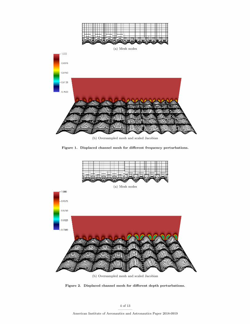
A. Boundary Roughness on channel

In the first test case we consider using the linear-elasticity approach to generate meshes with higher-ordercurved boundaries given an initial linear mesh. In particular we use the elasticity approach to deform alinear mesh near the boundary of a channel in order to simulate surface roughness. Sinusoidal displacementof the channel surfaces is applied with varying depth and frequency of surface roughness. We solve for an8th-order displacement to generate the deformed mesh. In Figure 1 we present two meshes (split left/right)corresponding to displacements with different frequency of surface oscillations. Due to the high frequencyof the oscillations (1/4-1/3 times the Nyquist frequency for this mesh) the mesh quality “looks” poor whenplotting only the nodal values. Thus, we also over-sample the 8th-order geometry representation from themesh, from which it is evident that we recover a smooth representation of the boundary displacements.In Figure 1 we also present a quantitative assessment of mesh quality by plotting the scaled Jacobian ofthe deformed mesh. The elasticity based deformation results in a high quality mesh with a scaled Jacobiangreater than 0.75 everywhere in the domain domain. Figure 2 shows similar results using two different depthsof displacements at a fixed frequency. It is evident from the mismatch between the meshes for the shallow(left) and deep (right) displacements that the perturbations extend throughout the domain quite far fromthe boundary. Again, high-quality elements are generated by the linear-elasticity approach.

B. Low Pressure Turbine Cascade

The second test case we consider is using the elasticity approach to generate deformed surface meshes for alow pressure turbine (LPT) blade in order to simulate surface roughness. Starting with an initial 8th order

3 of 13

American Institute of Aeronautics and Astronautics Paper 2018-0919

(a) Mesh nodes

(b) Oversampled mesh and scaled Jacobian

Figure 1. Displaced channel mesh for different frequency perturbations.

(a) Mesh nodes

(b) Oversampled mesh and scaled Jacobian

Figure 2. Displaced channel mesh for different depth perturbations.

4 of 13

American Institute of Aeronautics and Astronautics Paper 2018-0919

curvilinear mesh surface normal purtubations are applied and we use the elasticity approach to propogatethe surface deformations into the domain. Once again we use the elasticity approach to solve for a temporallyfixed mesh displacement. Figure 3 shows the deformation applied at the surface of the turbine blade, as wellas the deformed mesh near the leading edge of the blade.

(a) Surface Deformation (b) Deformed Mesh

Figure 3. Surface deformation and deformed mesh for LPT blade

The perturbed mesh is used to discretize the compressible Navier-Stokes equations (details of the equa-tions solved are given in Section IV). Figure 4 shows snapshots of the corresponding Navier-Stokes simula-tions using the unperturbed and perturbed geometries.

(a) Smooth blade (b) Blade w/ Surface Roughness

Figure 4. Snapshot of Mach number from Navier-Stokes simulations of LPT blade with and without surfaceroughness

.

In the baseline smooth configuration a small separation bubble is evident on the suction side of theblade. With simulated surface roughness, the flow remains attached over the entire blade matching theexperimentally observed behaviour. Complete details of this test case and the effects of surface roughnessare presented in an upcoming article.25

5 of 13

American Institute of Aeronautics and Astronautics Paper 2018-0919

C. Rotating Box

The third test case we consider is a small box rotated within a larger box. This test case was previouslyused by Froehle and Persson22 to assess a nonlinear elasticity approach for mesh deformation. This test caseis intended to stress the elasticity approach to determine how large displacements may be applied while stillgenerating a valid mesh. The test case which involves embedding a box of size (0.2× 0.2) within a unit box(1× 1) and rotating the interior box until the resulting deformed mesh has an invalid element. We considerdisplacing 2nd, 4th and 8th order meshes with a fixed number of degrees of freedom. First we consider thelinear-elastic approach using a spatially constant Young’s modulus. Figure 5 shows initial 2nd, 4th and 8thorder meshes and the corresponding deformed meshes with rotation of 15 and 30. We colour the deformedmeshes using the scaled determinant of the deformed mesh. Using a spatially constant Young’s modulus,there is significant skewing of the elements near the corners of the inner box already at 15. At rotationangles greater than 20, invalid 8th order meshes are generated with inverted elements at the corners ofthe interior box. At lower orders, somewhat larger rotation angles may be applied while maintaining validelements. However, even at 2nd order, valid meshes cannot be generated with rotation angles greater than35.

Next we consider the spatially varying Young’s modulus used by Froehle and Persson.22 The Young’smodulus is given by:

E(x) = 1 +100

1 + (d(x)/d0)2(5)

where d0 = 0.05 and d(x) = max0.0,min(dist(x,Γin) − d0,dist(x,Γout) + 2d0). Here Γin and Γout arerespectively the inner and outer boundaries of the domain, while dist(x,Γi) denotes the distance to theboundary. With this spatially varying Young’s modulus the linear-elastic approach allows for much largermesh deformations than a constant Young’s modulus. Figure 6 shows the deformed mesh and correspondingdeterminant of the scaled Jacobian at rotations of 15, 30 and 45. By increasing the stiffness near theboundaries, essentially rigid body deformation occurs near the boundaries while larger deformations occuron the interior of the domain. With the variable coefficient, the elasticity approach is able to generatevalid 2nd and 4th order meshes with a rotation of 45, while at 8th order a valid mesh is generated forrotations of up to 40. We note that using a nonlinear elasticity approach, even larger displacements maybe possible,22 however the impact of the Young’s modulus is much more significant than switching to anonlinear approach. In particular, we found that using the nonlinear approach with a constant Young’smodulus allowed for significantly less rotation than simply changing the Young’s modulus. Additionallyswitching to a nonlinear approach make the resulting system extremely stiff and difficult to solve.19

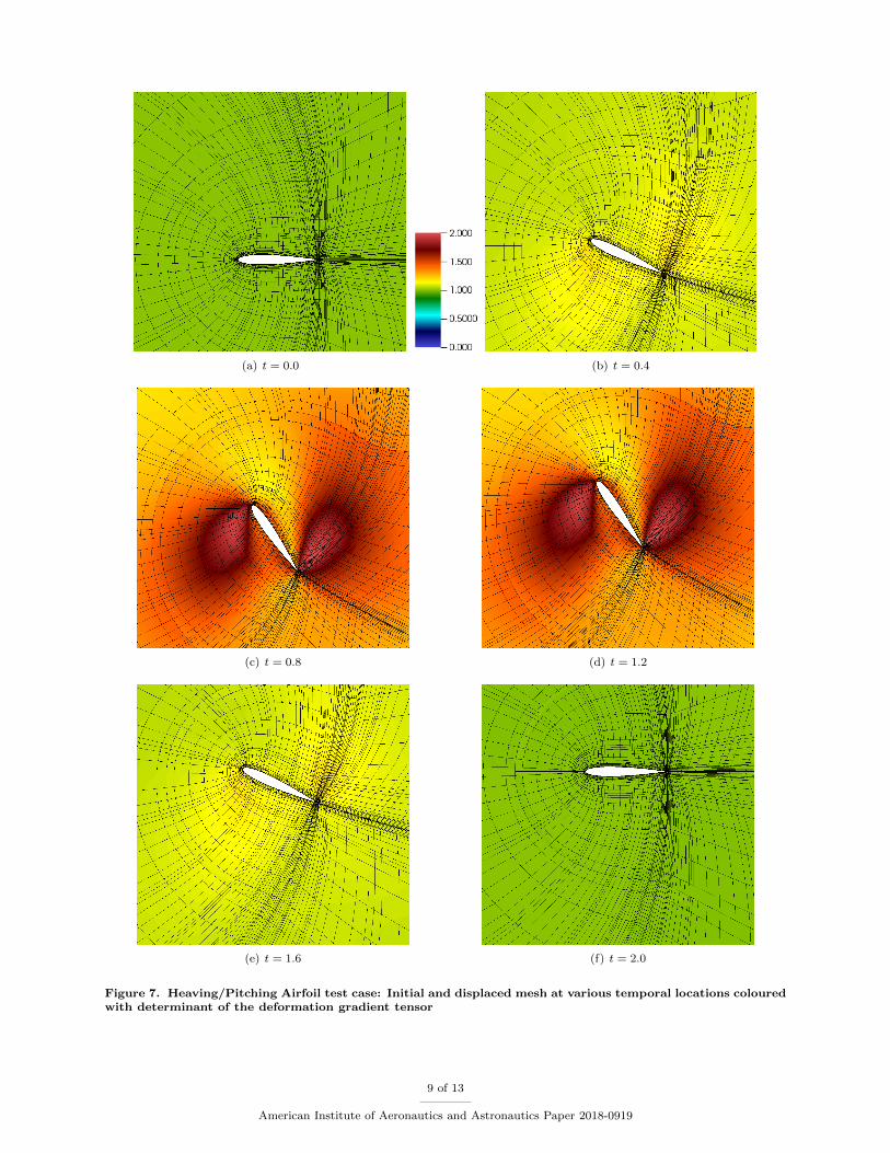
D. Heaving/Pitching Airfoil

The fourth test case we consider is generating a higher-order space-time mesh for a moving-body simulation.In particular, we consider one of the test cases from the Higher-Order Workshop.18 The test case involvesflow over the NACA0012 airfoil at M = 0.2, Re = 5000 initially at zero angle of attack with a prescribedheaving/pitching motion. In this case we solve for the space-time mesh velocity and recover the displacementby integrating the mesh velocity. Figure 7 depicts the initial 4th order mesh, along with the space-time meshdeformed using elasticity at several temporal locations throughout the heaving/pitching motion. Displacingthe interior nodes of the mesh the linear elastic model, with Poisson ratio of ν = 0.4 and Young’s modulusscaled with the inverse of the Jacobian determinant, ensures valid elements everywhere in the domain despitethe large deformations due to the prescribed motion. We quantify the quality of the mesh by plotting thedeterminant of the deformation gradient tensor near the surface of the airfoil. As can be seen, the linear-elastic model maintains high quality elements throughout the domain with the deformation tensor near 1everywhere in the domain except for some significant deformation near the trailing edge. We note as inthe previous test case, that using a constant Young’s modulus throughout the domain results in invalidelements. Similarly, using a Young’s modulus scaled inversely with the Jacobian determinant ensures nearrigid body motion near the airfoil surface as we generally have small elements here, while larger deformationsare allowed further from the airfoil surface where there are larger elements.

6 of 13

American Institute of Aeronautics and Astronautics Paper 2018-0919

(a) N = 2, θ = 0 (b) N = 4, θ = 0 (c) N = 8, θ = 0

(d) N = 2, θ = 15 (e) N = 4, θ = 15 (f) N = 8, θ = 15

(g) N = 2, θ = 30 (h) N = 4, θ = 30 (i) N = 8, θ = 30

Figure 5. Rotating box test case using constant Young’s modulus for different orders and angles of rotation.Meshes coloured by determinant of scaled Jacobian. (Note: for N = 4 and N = 8, grid depicts 2N quadraturepoints on each element)

7 of 13

American Institute of Aeronautics and Astronautics Paper 2018-0919

(a) N = 2, θ = 15 (b) N = 4, θ = 15 (c) N = 8, θ = 15

(d) N = 2, θ = 30 (e) N = 4, θ = 30 (f) N = 8, θ = 30

(g) N = 2, θ = 45 (h) N = 4, θ = 45 (i) N = 8, θ = 45

Figure 6. Rotating box test case using spatially varying Young’s modulus for different orders and angles ofrotation. Meshes coloured by determinant of scaled Jacobian. (Note: for N = 4 and N = 8, grid depicts 2Nquadrature points on each element)

8 of 13

American Institute of Aeronautics and Astronautics Paper 2018-0919

(a) t = 0.0 (b) t = 0.4

(c) t = 0.8 (d) t = 1.2

(e) t = 1.6 (f) t = 2.0

Figure 7. Heaving/Pitching Airfoil test case: Initial and displaced mesh at various temporal locations colouredwith determinant of the deformation gradient tensor

9 of 13

American Institute of Aeronautics and Astronautics Paper 2018-0919

IV. Coupled Results

In this section we couple the linear-elasticity approach with a compressible Navier-Stokes solver for fluiddynamics simulations.26 For the fluid domain we solve the compressible Navier-Stokes equations written inconservative form as

u,t +(F Inv − F V isc

),i

= 0, (6)

where u = [ρ, ρuj , ρE] is the conservative state vector, with ρ the density of the fluid, uj the velocitycomponents and E the total energy. The inviscid and viscous fluxes are given respectively by

F Inv =

ρui

ρujui + pδij

ρHui

F V isc =

0

τij

τijuj + κTT,j

(7)

where p is the static pressure, δij the Kronecker delta, H the total enthalpy, τij the viscous stress tensor, Tthe temperature and κT the thermal conductivity. The system is closed using the following relationships

T =p

ρR, p = (γ − 1)

(ρE − 1

2ρukuk

), τij = µ(ui,j + uj,i)− λuk,xk

δij , (8)

where R is the gas constant, γ the specific heat ratio, µ the dynamic viscosity and λ = 23µ the bulk viscosity.

We use a space-time discontinuous-Galerkin discretization of (6). We seek a solution u which satisfiesthe weak form∑κ

∫I

∫κ

−(w,tu + w,i(f

Ii − fVi )

)+

∫I

∫∂κ

w(f Iini − fVi ni) +

∫κ

w(tn+1− )u(tn+1

− )−w(tn+)u(tn−)

= 0 (9)

where the second and third integrals arise due to the spatial and temporal discontinuity, respectively, of the

basis functions. f Iini and fVi ni denote single valued numerical flux functions approximating, respectively,the inviscid and viscous fluxes at the spatial boundaries of the elements.

In a moving-body simulations there is only one-way coupling between the elasticity domain and the fluiddomain. We prescribe the motion, thus the elasticity solve is independent of the fluid domain. However, thefluid domain depends implicitly on the mesh deformation, as the integrals in (9) are over the deformed mesh.In the future we anticipate using this approach for performing fluid-structure interation, where the boundarydeformation will be prescribed by a structural model, which in turn will depend on the forces exerted by thefluid domain. Thus for this test case we solve the coupled elasticity/fluid problem simultaneously.

A. Isentropic Vortex Convection

In this test case we consider the isentropic convection of a vortex, while deforming the mesh with a prescribedmotion. The isentropic vortex convection problem is initialized with a perturbation about a uniform flowgiven by:

δu = −U∞βy − ycR

e−r2

2 (10)

δv = U∞βx− xcR

e−r2

2 (11)

δ

(P

ρ

)=

1

2

γ

γ − 1U2∞β

2e−r2

(12)

where U∞ is the convecting speed of the vortex, β is the vortex strength, R the characteristic radius, and(xc, yc) the vortex center. The exact solution to this flow is a pure convection of the vortex at speed U∞.

We consider a moving-body simulation with a mesh deformed to track the convection of the vortex anddeformed sinusoidally with boundary displacement given by:

x′ = x+ 0.1(x− xc) sin(π4 t) + U∞t (13)

y′ = y − 0.1(y − yc) sin(π4 t)ν(1− ν) (14)

10 of 13

American Institute of Aeronautics and Astronautics Paper 2018-0919

(a) t = 0.0 (b) t = 2.5 (c) t = 5.0

(d) t = 7.5 (e) t = 10.0

Figure 8. Deformed mesh and fluid solution on original mesh for isentropic vortex convection problem

11 of 13

American Institute of Aeronautics and Astronautics Paper 2018-0919

Figure 8 depicts the displaced mesh through one cycle of deformation and the corresponding vortexplotted in the original (as opposed to the displaced) coordinate system. As can be seen, the coupled space-time finite-element method maintains a high-quality solution through one cycle of mesh motion.

We note that solving the coupled elasticity-fluid problem is significantly harder than solving the elasticityor the fluid independently. There are several challenges in solving the coupled problem that need to beaddressed before this methodology can be applied to more complex problems. In particular, we note thatthe stiffness of the space-time elasticity problem is independent of the time-step (as we drop all temporalterms this is essentially a “steady” solve), while the stiffness of the fluid solve decreases with time step.Thus even for very small time-steps the elasticity solve requires efficient preconditioning to be practical.Furthurmore, partially converged elasticity solutions may result in mesh deformations with invalid elements(even if the converged solution is valid), resulting in non-physical residual evaluations on the fluid domain.Thus a sophisticated globalization strategy is required. Currently, a pseudo-transient type globalizationstrategy is employed for the fluid domain, while no globalization strategy is used for the elasticity domain.The combination of the different preconditioning and globalization strategies on the two domains results insome non-intuitive convergence behaviour such as poorer convergence when decreasing the time step. It isanticipated that improving the preconditioning and extending the globalization strategy for the elasticitydomain will significantly improve the solver performance.

V. Outlook/Future Work

In this paper we have presented a linear elastic solution strategy for higher-order space-time mesh defor-mation, and demonstrated the application of this strategy for some simple problems. The elasticity approachwas shown to be appropriate for generating higher-order meshes for fixed-grid simulations and higher-orderspace-time meshes for use in moving-body fluid dynamics simulations. In our initial approach we haveapplied a very simple solution strategy which involved no preconditioning or globalization. Applicationof this approach for coupled fluid-structure applications will require addressing these limitations. Futureapplications will focus on coupling the fluid solve and mesh deformation to a structural model.

References

1Diosady, L. T. and Murman, S. M., “Design of a variational multiscale method for turbulent compressible flows,” AIAAPaper 2013-2870, 2013.

2Diosady, L. T. and Murman, S. M., “DNS of flows over periodic hills using a discontinuous Galerkin spectral elementmethod,” AIAA Paper 2014-2784, 2014.

3Diosady, L. T. and Murman, S. M., “Tensor-Product Preconditioners for Higher-order Space-Time Discontinuous GalerkinMethods,” 2014, under review.

4Diosady, L. T. and Murman, S. M., “Higher-Order Methods for Compressible Turbulent Flows Using Entropy Variables,”AIAA Paper 2015-0294, 2015.

5Ceze, M., Diosady, L., and Murman, S., “Development of a High-Order Space-Time Matrix-Free Adjoint Solver,” AIAA2016-0833, 2016.

6Burgess, N. K., Diosady, L. T., and Murman, S. M., “A C1-discontinuous-Galerkin Spectral-element Shell StructuralSolver,” AIAA Paper 2017-3727, 2017.

7Hubner, B., Walhorn, E., and Dinkler, D., “A monolithic approach to fluid-structure interaction using space-time finiteelements,” Comput. Methods Appl. Mech. Engrg., Vol. 2004, 2004, pp. 2087–2104.

8Klaij, C., van der Vegt, J., and van der Ven, H., “Spacetime discontinuous Galerkin method for the compressible Navier-Stokes equations,” Journal of Computational Physics, Vol. 217, 2006, pp. 589611.

9Heil, M., Hazel, A. L., and Boyle, J., “Solvers for large-displacement fluidstructure interaction problems: segregatedversus monolithic approaches,” Computational Mechanics, Vol. 43, 2008, pp. 91–101.

10van Brummelen, E., Hulshoff, S., and de Borst, R., “A monolithic approach to fluid-structure interaction using space-timefinite elements,” Comput. Methods Appl. Mech. Engrg., Vol. 2003, 2003, pp. 2727–2748.

11K. Stein, T. T. and Benney, R., “Mesh Moving Techniques for Fluid-Structure Interactions With Large Displacements,”J. Appl. Mech, Vol. 70, No. 1, 2003, pp. 58–63.

12Tezduyar, T. E. and Sathe, S., “Modelling of fluid-structure interactions with the space-time finite elements: Solutiontechniques,” Int. J. Numer. Meth. Fluids, Vol. 54, 2007, pp. 855–900.

13Wang, L. and Persson, P.-O., “A high-order discontinuous Galerkin method with unstructured space-time meshes fortwo-dimensional compressible flows on domains with large deformations,” Computers and Fluids, Vol. 118, 2015, pp. 53–68.

14Lesoinne, M. and Farhat, C., “Geometric conservation laws for flow problems with moving boundaries and deformablemeshes, and their impact on aeroelastic computations,” Comput. Methods Appl. Mech. Engrg., Vol. 134, 1996, pp. 71–90.

15Yano, M., An Optimization Framework for Adaptive Higher-Order Discretizations of Partial Differential Equations onAnisotropic Simplex Meshes, Ph.D. thesis, MIT, 2009.

12 of 13

American Institute of Aeronautics and Astronautics Paper 2018-0919

16Yang, Z. and Mavriplis, D. J., “A Mesh Deformation Strategy Optimized by the Adjoint Method on Unstructuredmeshes,” AIAA Paper 2007-0557, 2007.

17Barth, T. J., “Numerical Methods for Gasdynamic Systems on Unstructured Meshes,” An Introduction to Recent Devel-opments in Theory and Numerics for Conservation Laws, edited by D. Kroner, M. Olhberger, and C. Rohde, Springer-Verlag,1999, pp. 195 – 282.

18Wang, Z., Fidkowski, K., Abgrall, R., Bassi, F., Caraeni, D., Cary, A., Deconinck, H., Hartmann, R., Hillewaert, K.,Huynh, H., Kroll, N., May, G., Persson, P.-O., van Leer, B., and Visbal, M., “High-Order CFD Methods: Current Status andPerspective,” International Journal for Numerical Methods in Fluids, Vol. 72, 2013, pp. 811–845.

19Persson, P.-O. and Peraire, J., “Curved Mesh Generation and Mesh Refinement using Lagrangian Solid Mechanics,”AIAA Paper AIAA-2009-0949, 2009.

20Moxey, D., Ekelschot, D., Keskin, ., Sherwin, S., and Peiro, J., “A Thermo-elastic Analogy for High-order CurvilinearMeshing with Control of Mesh Validity and Quality,” Procedia Engineering, Vol. 82, 2014, pp. 127–135.

21Moxey, D., Ekelschot, D., Keskin, U., Sherwin, S., and Peiro, J., “High-order curvilinear meshing using a thermo-elasticanalogy,” Computer-Aided Design, Vol. 72, 2016, pp. 130–139.

22Froehle, B. and Persson, P., “Nonlinear Elasticity for Mesh Deformation with High-Order Discontinuous Galerkin Methodsfor the Navier-Stokes Equations on Deforming Domains,” Spectral and High Order Methods for Partial Differential EquationsICOSAHOM 2014 , edited by R. Kirby, M. Berzins, and J. Hesthaven, 2015.

23Karniadakis, G. and Sherwin, S., Spectral/hp element methods for CFD , Oxford University Press, New York, NY, 1999.24Lynch, R. E., Rice, J. R., and Thomas, D. H., “Direct solution of partial difference equations by tensor product methods,”

Numerische Mathematik , Vol. 6, No. 1, 1964, pp. 185–199.25Garai, A., Diosady, L., Murman, S., and Madavan, N., “Scale-Resolving Simulations of Low-Pressure Turbine Cas-

cades with Wall Roughness Using a Spectral-Element Method,” Proceedings of the ASME Turbo Expo 2018: TurbomachineryTechnical Conference and Exposition, No. GT2018-75982, 2018.

26Wiart, C. C. D., Diosady, L. T., Garai, A., Burgess, N., Blonigan, P., Ekelschot, D., and Murman, S. M., “Design of amodular monolithic implicit solver for multi-physics applications,” AIAA Paper 2018-1400, 2018.

13 of 13

American Institute of Aeronautics and Astronautics Paper 2018-0919