A Learning-based Model of Repeated Games

with Incomplete Information

Juin-Kuan Chong

The NUS Business School, National University of Singaporebizcjk@nus.edu.sg

Colin F. Camerer

Division of Humanities and Social Sciences, California Institute of Technology,Pasadena, CA 91125

camerer@hss.caltech.edu

Teck H. Ho

Haas School of Business, University of California, Berkeleyhoteck@haas.berkeley.edu

Abstract

This paper tests a learning-based model of strategic teaching in repeated gameswith incomplete information. The repeated game has a long-run player whose typeis unknown to a group of short-run players. The proposed model assumes a fractionof ‘short-run’ players follow a one-parameter learning model (self-tuning EWA). Inaddition, some ‘long-run’ players are myopic while others are sophisticated and ra-tionally anticipate how short-run players adjust their actions over time and “teach”the short-run players to maximize their long-run payoffs. All players optimize nois-ily. The proposed model nests an agent-based quantal-response equilibrium (AQRE)and the standard equilibrium models as special cases. Using data from 28 experi-mental sessions of trust and entry repeated games, including 8 previously unpub-lished sessions, the model fits substantially better than chance and much better thanstandard equilibrium models. Estimates show that most of the long-run players aresophisticated, and short-run players become more sophisticated with experience.

Key words: repeated games, self-tuning experience-weighted attraction learning,quantal response equilibrium

1 This research was supported by NSF grant SES-0078911. Thanks to John Kagel

Preprint submitted to Elsevier Science 11 February 2005

1 Introduction

Many transactions in the economy are conducted repeatedly by players who ei-ther know the history of behavior by others and anticipate future interactions.Examples include cartels, employment relations, merchant banking relation-ships, long-standing corporate rivalries, customers who are loyal to retailers,lending to customers with known credit histories, and so forth. Game theo-rists model these situations as repeated games with incomplete informationand study their sequential equilibria (SE).

Two early experimental studies evaluated the accuracy of SE predictions inrepeated trust games (Camerer and Weigelt (1988a)) and entry deterrencegames (Jung, Kagel, and Levin (1994)). In these games, a long-run player ismatched repeatedly with a group of short-run players. The long-run playercan be one of the two types (normal or special). The short-run players knowthe proportions of the two types, but do not know which type of the long-runplayer they face.

In the trust game, a single borrower B (i.e., the long-run player) wants toborrow money from a series of 8 lenders denoted Li (i = 1, . . . , 8) (i.e., theshort-run players) (cf. Kreps (1990)). A lender makes only a single lendingdecision (either Loan or No Loan). The borrower makes a string of decisions,(either Repay or Default), each time a lender chooses Loan.

The entry game deterrence is similar. A series of eight short-run entrants eachdecide, one at a time, whether to enter or stay out in a series of periods. Ifthe entrant enters in a period, a long-run incumbent decides whether to fightor share.

The payoffs in the trust game imply that if the games were only one stage, theborrower would Default; anticipating this, the rational lender would choose NoLoan. Similarly, in a one-stage entry deterrence game the entrant would enterbecause she would anticipate that the incumbent would share. The specialtypes of borrowers and incumbents have payoffs which create a preference forrepaying or fighting, respectively, rather than defaulting or sharing.

Both experimental studies showed three empirical regularities:

for rapidly supplying data and to Drew Fudenberg, Qi-Zheng Ho, David Hsia, XinWang, and four referees, for discussions and help. Useful comments were receivedfrom seminar participants at Berkeley, Caltech, Chicago, Harvard, Hong Kong UST,New York University, Pittsburgh, Princeton, and Wharton. We would also like tothank the editors and two anonymous reviewers for their helpful comments andsuggestions

2

(1) The basic patterns predicted by SE occur in the data: In the trust game,borrowers are more likely to default in later rounds than in earlier rounds,and lending rates fall after a previous default. Similarly, incumbents aremore likely to share in later rounds, and entry rates increase after sharing.

(2) There are two systematic deviations from the SE predictions: (a) Thereare too few defaults (by borrowers) and too few fights (by incumbents);and (b) the predicted rates of lending and entering increasing smoothlyacross rounds, while the SE predicts a step function across periods.

(3) In the experiments, subjects played 50-100 eight period sequences. Equi-libration occurred across sequences (”cross-sequence learning”) and be-tween experimental sessions (experienced subjects were closer to SE thaninexperienced subjects).

Camerer and Weigelt (1988a) and Jung et al. (1994) showed that the SEprediction could be modified to explain both the basic patterns (1) and thedeviation (2a) above by assuming that some proportion of normal-type playersacted like the special types induced by the experimenter (the “home-madeprior”).

These early analyses fell short in three ways: First, the prior was inferred fromthe data rather than measured separately in one-stage games. Second, the SEpredictions of trust and entry rely on two different special types of oppositebehavioral kinds– one is trustworthy (sacrificing money to help others) and theother is vindictive (sacrificing money to harm others). Third, the modified SEmodel with a homemade prior cannot explain deviation (2b) and the cross-sequence learning (3). Authors of both studies recognize that the modifiedSE model cannot explain cross-sequence learning. As (Camerer and Weigelt,1988a, p. 27-28) note 2 :

“...the long period of disequilibrium behavior early in these experimentsraises the important question of how people learn to play complicated games.The data could be fit to statistical learning models (e.g., Selten and Stoecker(1986)), though new experiments or new models might be needed to explainlearning adequately.”

Responding to Camerer and Weigelt’s call for new learning models, this paperdevelops and estimates a learning-based model with strategic ”teaching”. Inthe model, a fraction of short-run players learn adaptively from experienceand the rest are ”sophisticated” 3 – they rationally anticipate how the long-

2 And see (Jung et al., 1994, p. 90)3 See Selten (1991), Milgrom and Roberts (1991), and Fudenberg and Kreps (1990)for models of sophistication. Adding sophistication to adaptive learning makes sensebecause long-run player subjects often have a sense that short-run players are learn-ing. Models with sophistication also predict that players care about the payoffs ofothers, and how they are matched with partners in the future (adaptive learning

3

run players learn and behave. Similarly, a fraction of long-run players aresophisticated and the rest are myopic (they act as if they are playing a one-stage game). In repeated games with partner matching, sophisticated long-runplayers have an incentive to “teach” the short-run learners what to expect.This kind of “strategic teaching” has been proposed as a boundedly rationaltheory of reputation formation (see Fudenberg and Levine (1989), Watson(1993) and Watson and Battigali (1997)). Camerer et al. (2002) offer the firstempirical implementation of such a model using data from repeated trustgames. 4

This general model both extends simple adaptive learning models, by addingsophistication, and weakens equilibrium models, by adding learning. Becausethe model mixes adaptive and sophisticated types, certain parameter restric-tions reduce the model to boundary cases of special interest. Purely adaptivelearning is one boundary case. When all players are sophisticated, believe allothers are sophisticated, and best-respond, the model reduces to simply an-other boundary case – Bayesian Nash equilibrium. We study an Agent Quan-tal Response Equilibrium (AQRE) version of Bayesian-Nash equilibrium. InAQRE, players optimize noisily but update their beliefs using Bayes’ rule andanticipate accurately what others will do (McKelvey and Palfrey (1998)).

Adding adaptive players make sense because there are behavioral differencesbetween sophisticated and adaptive players. Consider the lender in the trustgames. Adaptive lenders will continue lending until a default occurs, afterwhich later lenders are less likely to lend. A sophisticated lender, in contrast,anticipates default by assessing the probability of the borrower being a normal(“dishonest”) type. Hence she will stop lending when the posterior probabilityof dishonest type is high enough that the expected payoff from lending exceedsnot lending. This could happen even without a default in previous rounds. Inshort, adaptive players react to past default behavior but sophisticated playersanticipate future default behavior.

The general model has the potential to improve the modified SE used in earlierpapers, which fell short in three ways:

models don’t have these properties), consistent with experimental evidence (Partowand Schotter (1993), Mookherjee and Sopher (1994), Cachon and Camerer (1996),Andreoni and Miller (1993)). Models including sophistication have generally fit bet-ter in matrix games, signaling games, repeated trust games, and p-beauty contestgames (see Stahl (1999), Cooper and Kagel (2001), Camerer, Ho, and Chong (2002),Ho, Camerer, and Weigelt (1998)).4 Their model consists solely of adaptive short run players who follow a parametricEWA model (which requires a total of 18 parameters). They do not allow their longrun players to be a special home-made type. However, the special home-made typeis estimated in the benchmark AQRE model. The models are validated on one trustgame dataset from Camerer and Weigelt (1988a).

4

First, the value of the home-made prior is measured separately, in one-stageexperiments where potential reputation effect is absent, rather than estimatedfrom the repeated games.

Second, the model provides a unifying theory of ”special types” across differentgames. Both types of special-type players– trustworthy borrowers and fightinglenders– act like Stackelberg players: They choose the strategy they wouldcommit to, if they could, in order to improve long-run payoffs. (This is theessence of the models of Fudenberg and Levine (1989)) Our model derivesthe two different types endogenously from the game payoff structures and asingle common source: Both are special types whose behavior is similar tothat of sophisticated long-run players who maximize long-run payoffs. Eventhough the impact of teaching is quite different between trust and entry games(payback in trust game is mutually beneficial while fighting in entry game isprivately beneficial), the model captures both impacts across games with noadditional parameter.

Third, although switching from SE to AQRE improves fit and explains thedeviation (2b), it cannot explain learning across sequences within an exper-imental session, and learning across sessions, which the general model can.Cross-sequence learning can be explained by allowing subjects to learn bothfrom previous periods within an eight-period sequence, and from previouseight-period sequences.

In this paper, we apply the general model to the 20 experimental sessionspublished earlier on trust and entry deterrence games, and to 8 brand newsessions. The new data provide additional replication of the basic patternsand give us more statistical power. We estimate that more than 90% of thelong-run players in both games are sophisticated. About half of the short-run players are estimated to be sophisticated in sessions with inexperiencedsubjects, but all the short-run players are estimated to be sophisticated afterexperience.

To verify that the general model captures the trends in the data and to un-derstand the impact of each feature of the model in tracking the data, wesimulate the behavior of the model under various parameter restrictions (i.e.,after ”disabling” features one at a time) and compare with the data.

The three empirical regularities discussed above can be translated into cross-round trends and cross-sequence trends. We find that the model tracks datawell in both cross-round and cross-sequence trends: when there is a significanttrend in the data, the model picks up the trend as well.

We disable four key features of the model one at a time: cross-sequence learn-ing, the proportion of sophisticated lenders, the home-made prior, and theproportion of sophisticated borrowers. And we find that disabling the features

5

has significant impact on the ability of the model to pick up the trends in thedata. In some cases, the prediction of the restriction model either does notpick up the trend at all or predicts an opposite trend.

The next section introduces the model of repeated games and reports newexperiments that measure the proportions of special types. Section 3 discussesthe key differences among equilibrium,AQRE and the proposed model. Section4 reports estimates of the models on three data sets from repeated trust andentry-deterrence games. Section 5 checks the robustness of the model throughsimulation. Section 6 concludes.

2 A Model of Repeated Games

We consider any two-player repeated game with incomplete information, wherethe long-run player can be one of two types (or equivalently, have one of thetwo induced payoff functions) and short-run player is uncertain about long-run player’s type. In repeated borrower-lender trust relationships, a lenderis uncertain about whether a borrower is honest or dishonest. In repeatedincumbent-entry games, an entrant is uncertain whether an incumbent willalways fight entry or not. We refer to the honest borrowers and aggressiveborrowers as special types. Standard equilibrium analysis assumes both playersare sophisticated and behave according to the prediction of Bayesian Nashequilibrium.

Table 1 shows the various player segments in the proposed model. p fraction oflong-run players are induced to be special type and (1−p) fraction to be normaltype. Of the normal type players, a fraction θ has an inherent preference forspecial type’s payoff function, a fraction (1 − θ) · αB are sophisticated anda fraction (1 − θ) · αB are myopic. A αL fraction of short-run players aresophisticated and the remaining 1 − αL are adaptive. If αL = αB = 1, themodel reduces to AQRE. If αL = αB = 0, the model reduces to the self-tuningEWA learning model.

The proposed model allows a fraction θ of long-run player’s with normal-typepayoff to act like the special-type payoff (this fraction is previously labeled ashomemade prior). Along with the fraction p of the borrower players who areinduced to behave like special types by the experimenter, the total fractionwho actually behave like special types is p + (1− p)θ.

Earlier experiments imputed a value for the homemade prior (Camerer andWeigelt (1988a), Neral and Ochs (1992)) or estimated it from a structuralmodel (Palfrey and Rosenthal (1988), McKelvey and Palfrey (1992)). We mea-sured the frequency of homemade prior in two separate experimental sessions

6

with one-shot games with random rematching (using the same subject poolsused in the early trust experiments). In these games, there is no reputationalincentive for behaving like special type players. The measured rate of thosebehaviors is then used to constrain their frequency in the repeated game esti-mation.

In a typical experimental session, subjects are randomly assigned fixed rolesof borrower, or lender (e.g., 11 subjects are divided into 3 borrowers and 8lenders). In a single sequence, a borrower B is randomly chosen to play in allthe periods of an eight-period supergame (the other borrowers sit and watch).In addition, the borrower may be payoff-induced to be an honest type withprobability p where p is set by the experimenter a priori. A borrower typeremains the same for all 8 periods of the sequence. Each lender Li plays inexactly one of the 8 stage games in each supergame in a random position eachtime (the position of a particular lender-subject in each sequence is unknownto the borrower). The entire eight-stage supergame is repeated in a series ofsequences (typically 50 to 100 sequences).

We model the choice probabilities of each segment f (f assumes a value ofa for adaptive learner and a value of s for sophisticated player) of players attime t. In specifying the probability, we adopt the logistic approach in whichlenders of segment f attach an attraction value Aj

L(f, k, t) to each strategyj in a given round t of a sequence k. Similarly, borrowers of segment f ′ (f ′

assumes a value of m for myopic player, a value of s for sophisticated player,and a value of h if the borrower behaves like an honest type) have an attractionvalue Aj

B(f′, k, t) to each strategy j in a given round t of a sequence k. Below,

we will discuss how AjL(f, k, t) and Aj

B(f′, k, t)(i = L,B) are determined for

each segment of the players in Table 1.

2.1 Adaptive Lenders

Recall that lenders play only once in each sequence. Yet they clearly respondto the experiences of the other players, which they only observe. So we assume“observational learning”: Players can learn from previous rounds in a sequenceand from previous sequences. Consider round 7 in sequence 14. The round 7lender who is deciding what to do saw what happened in the previous 6 roundsof sequence 14, and learned about the attractiveness of lending from whathappened in those rounds. But the lender also knows what happened in theupcoming (7th) round of the previous sequences 1-13 –a glance at the past–and learned about whether she should loan in round 7 from those previousround 7 experiences. We call the latter effect cross-sequence learning.

Within-sequence learning can be modeled by standard learning theories. We

7

use a “self-tuning” EWA model of Ho, Camerer, and Chong (2004) for itsparsimony (with only 1 parameter) and versatility (it has predicted reasonablyaccurately in other games). (Other adaptive models could be used in its placeas well).

Returning to our example, the strategy loan for a lender before period 7 ofsequence 14 is influenced by two sources of experience –the attraction of loanafter period 6 of sequence 14, and the experience after choosing loan in period7 of sequences 1-13. These influences are captured by differentially updatingthe attractions of the strategies.

The strength of cross-sequence learning is parameterized by a parameter τ . Ifτ = 0 there is no cross-sequence learning; if τ = 1 experience in upcomingperiods of previous sequences is just as important as experience in the previousperiod of the current sequence. The data will tell us how strong cross-sequencelearning is through the value of τ .

The updating of the attraction for an adaptive lender AjL(a, k, t) occurs in 2

steps. The idea is to create an “interim” attraction for round t, BjL(a, k, t),

based on the attraction AjL(a, k, t − 1) and payoff from the round t, then

incorporate experience in round t + 1 from previous sequences, transformingBj

L(a, k, t) into a final attraction AjL(a, k, t). The exact specification of the

attraction updating is as follows:

(1) Learning across rounds within a sequence:

BjL(a, k, t)=

φ(k, t) ·N(k, t− 1) · AjL(a, k, t− 1)

M(k, t)

+[δj(k, t) + [1− δj(k, t)] · I(j, sL(k, t))]πL(j, sB(k, t))

M(k, t)(1)

M(k, t)=φ(k, t) ·N(k, t− 1) + 1 (2)

where φ(k, t) and δ(k, t) are functional parameters and N(k, 0) = 1, asspecified in Ho et al. (2004) (see Appendix for further details). 5 The ini-tial attraction Aj

L(a, k, 0) = A0(No Loan/Not Enter) for the strategy j =No Loan (Not Enter) is estimated. I(j, sL(k, t)) is the indicator function

5 In Camerer et al. (2002), adaptive short run players follows a parametric EWAmodel with a fixed set of parameter estimates. Having a fixed set of learning pa-rameters restricts model flexibility. It seem reasonable to assume that the adaptiveplayer relies less on her past learning experience when she senses that her past ex-perience does not help (lending no longer seems that attractive when more defaultsare happening). The reliability of past experience does deteriorate in later roundswhen default happens more often. Having fixed parameters hinders this learningflexibility.

8

that equals 1 if strategy j is the chosen strategy sL(k, t) of lender L inround t of sequence k, and equals 0 otherwise.

(2) Learning in a coming round from previous sequences:

AjL(a, k, t)=

φ(k, t)τ ·M(k, t) · BjL(a, k, t) + τ · δ(k, t)πj

L(k, t+ 1)

N(k, t)(3)

N(k, t)= φ(k, t)τ ·M(k, t) + τ (4)

where we assume that the learning about an upcoming round t fromprevious sequences is driven by the average payoff in the round t’s in allprevious sequences (i.e., πj

L(k, t+1) =∑k−1

m=1 πL(j, sB(m, t+1))/(k− 1)).

The attraction at the end of time period t then determines the predictedadaptive lender’s choice probability at t+ 1 according to the logit rule,

P jL(a, k, t+ 1) =

eλaL·Aj

L(a,k,t)

∑j′ e

λaL·Aj′

L (a,k,t). (5)

2.2 Sophisticated Lenders

The sophisticated lender rationally anticipates the action of the borrower andmaximizes her own expected payoff in each period. Let the lender’s belief aboutthe overall fraction of honest types at sequence k and end of time t be r(k, t).Then, the remaining fraction (1 − r(k, t)) of borrowers are either myopic orsophisticated. Their combined predicted probability of choosing strategy j′ att+ 1 is as follows: P j′

B (d, k, t+ 1) = [(1− αB) · P j′B (m) + αB · P j′

B (s, k, t+ 1)].The expected payoff of lender for choosing strategy j is then given by:

AjL(s, k, t)=

∑j′

[(1− r(k, t))P j′

B (d, k, t+ 1) + r(k, t)P j′B (h)

]πL(j, j

′) (6)

where πL(j, j′) is the lender’s payoff for strategy j when borrower chooses j′.

P j′B (h) is the probability that an honest borrower chooses strategy j′. 6

If the sophisticated lender chooses loan, she updates her belief in a Bayesianmanner at the end of t+1 using the borrower’s choice probabilities as follows:

6 Notice that P j′B (h) does not depend on arguments k and t because the probability

does not vary across periods.

9

r(k, t+ 1)=P j′

B (h) · r(k, t)P j′

B (h) · r(k, t) + P j′B (d, k, t+ 1) · (1− r(k, t))

(7)

where j′ is the chosen strategy.

If the lender chooses noloan, then r(k, t + 1) = r(k, t). Each lender starts atround 1 with the prior P(Honest), or r(k, 1) = p+ (1− p)θ.

Updating the belief r(k, t) changes the attractions AjL(s, k, t) and captures

learning. The updated attraction determines the sophisticated lender’s choiceprobability according to the logit rule,

P jL(s, k, t+ 1) =

eλsL·Aj

L(s,k,t)

∑j′ e

λsL·Aj′

L(s,k,t)

. (8)

2.3 Honest Borrowers

Honest borrowers always earn more from repaying (by definition). They chooseaccording to the stage game payoffs of honest type conditional on loan by thelender using a logit rule as follows:

P jB(h) =

eλhB·πH(j,Loan)

∑j′ e

λhB·πH(j′,Loan)

. (9)

2.4 Myopic Borrowers

Since borrowers move after the lenders do, there is nothing for a borrower tolearn. We call the borrowers who care only about immediate payoff “myopic”.The attractions of repay and default are simply the stage-game payoffs ofdishonest type conditional on loan by the lender. They choose between thosestrategies using a logit rule:

P jB(m) =

eλmB ·πD(j,Loan)

∑j′ e

λmB·πD(j′,Loan)

(10)

10

2.5 Sophisticated Borrowers

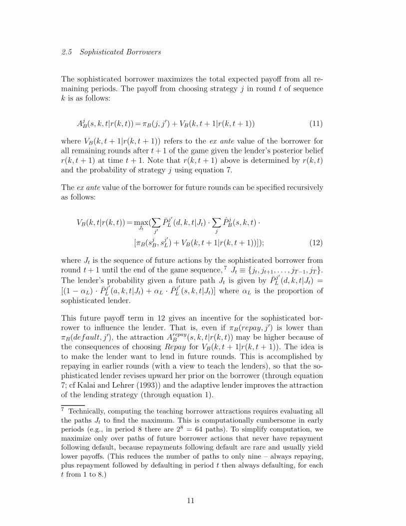
The sophisticated borrower maximizes the total expected payoff from all re-maining periods. The payoff from choosing strategy j in round t of sequencek is as follows:

AjB(s, k, t|r(k, t))=πB(j, j

′) + VB(k, t+ 1|r(k, t+ 1)) (11)

where VB(k, t + 1|r(k, t + 1)) refers to the ex ante value of the borrower forall remaining rounds after t+1 of the game given the lender’s posterior beliefr(k, t + 1) at time t + 1. Note that r(k, t + 1) above is determined by r(k, t)and the probability of strategy j using equation 7.

The ex ante value of the borrower for future rounds can be specified recursivelyas follows:

VB(k, t|r(k, t))=maxJt

(∑j′

P j′L (d, k, t|Jt) ·

∑j

P jB(s, k, t) ·

[πB(sjB , s

j′L) + VB(k, t+ 1|r(k, t+ 1))]); (12)

where Jt is the sequence of future actions by the sophisticated borrower fromround t+ 1 until the end of the game sequence, 7 Jt ≡ {jt, jt+1, . . . , jT−1, jT}.The lender’s probability given a future path Jt is given by P j′

L (d, k, t|Jt) =

[(1 − αL) · P j′L (a, k, t|Jt) + αL · P j′

L (s, k, t|Jt)] where αL is the proportion ofsophisticated lender.

This future payoff term in 12 gives an incentive for the sophisticated bor-rower to influence the lender. That is, even if πB(repay, j

′) is lower thanπB(default, j

′), the attraction ArepayB (s, k, t|r(k, t)) may be higher because of

the consequences of choosing Repay for VB(k, t + 1|r(k, t + 1)). The idea isto make the lender want to lend in future rounds. This is accomplished byrepaying in earlier rounds (with a view to teach the lenders), so that the so-phisticated lender revises upward her prior on the borrower (through equation7; cf Kalai and Lehrer (1993)) and the adaptive lender improves the attractionof the lending strategy (through equation 1).

7 Technically, computing the teaching borrower attractions requires evaluating allthe paths Jt to find the maximum. This is computationally cumbersome in earlyperiods (e.g., in period 8 there are 28 = 64 paths). To simplify computation, wemaximize only over paths of future borrower actions that never have repaymentfollowing default, because repayments following default are rare and usually yieldlower payoffs. (This reduces the number of paths to only nine – always repaying,plus repayment followed by defaulting in period t then always defaulting, for eacht from 1 to 8.)

11

The final attraction then determines the lender’s choice probability accordingto the logit rule,

P jB(s, k, t+ 1) =

eλsB·Aj

B(s,k,t)

∑j′ e

λsB·Aj′

B(s,k,t). (13)

2.6 Likelihood and Estimation

The models are estimated using 3 datasets: two trust game datasets fromCamerer and Weigelt (1988a,b) and one entry deterrence dataset from Junget al. (1994). All experimental sessions within a dataset are restricted to have acommon set of parameters (except for the scale sensitivity parameters λs whereeach session has its own). Maximum likelihood estimation (MLE) was usedto calibrate the model on 70% of the sequences in each experimental session,then forecast behavior in the remaining 30% of the sequences in that session.If the model fits in-sample purely by overfitting, it will perform surprisinglypoorly out-of-sample.

The likelihood function used in estimation consists of three parts:

(1) The likelihood of observing the data of the lenders is as follows:

LL = [(1− αL) · ΠkΠtPsL(k,t)L (a, k, t) + αL · ΠkΠtP

sL(k,t)L (s, k, t)] (14)

where sL(k, t) is the strategy actually chosen by lender L at time t insequence k.

(2) For the sequences where an honest-type borrower is drawn (with prob-ability p), the likelihood of observing the data of the borrowers is asfollows:

LHB = Πk”ΠtP

sB(k”,t)B (h) (15)

where k” are the sequences with honest types and sB(k”, t) is the strategychosen by the borrower at time t in sequence k”

(3) For the sequences where an dishonest-type is drawn, the likelihood ofobserving the data of the borrowers is as follows:

LDB = θ · Πk′ΠtP

sB(k′,t)B (h) + (1− θ) ·

[(1− αB) · Πk′ΠtP

sB(k′,t)B (m)

+αB · Πk′ΠtPsB(k′,t)B (s, k′, t)

](16)

where k′ are the sequences with dishonest-type draws and sB(k′, t) is the

strategy chosen by the borrower at time t in sequence k′.

12

Finally, the total likelihood of observing all the data is given by LL · LHB · LD

B .

2.7 Measuring the Homemade Prior θ Experimentally

Earlier trust and entry experiments showed that even when the induced frac-tion of honest borrowers or fighter types is zero, there is a substantial re-payment and fighting in finite games (even in the last period). Inspired bythe “gang of four” model of Kreps and Wilson (1982), Camerer and Weigelt(1988a) suggested this was due to the presence of an endogenous fraction ofsubjects who, despite monetary incentives to default, simply preferred to actreciprocally and repay– a “homemade prior” of reciprocal types. Palfrey andRosenthal (1988) used the same idea to explain contribution in public goodsgames. 8

In Camerer et al. (2002), the homemade prior θ is estimated from the data aspart of fitting a QRE model. The resulting estimates were high– from .5 to1– compared to the values around .1-.2 suggested by early experiments. Thisprobably means the QRE model needs to overestimate θ in order to make upfor some other basic misspecification.

Since the homemade prior is intimately tied to the extent of repaying or fight-ing, it is important to estimate it precisely and plausibly. By definition, honestor aggressive types will repay or fight even in one-shot games (their behav-ior springs from preferences, not strategy). Therefore, we recently measured θby conducting two experimental sessions of one-shot games, reproducing theoriginal experimental conditions 9 from repeated games as closely as possiblewhile generating enough data for a reliable estimate.

One session used the most common payoff structure in trust games and theother session used the most common structure in entry games (see Table 2). 10

Each session used 12 subjects playing two blocks of 6 rounds in a fixed-roleprotocol (as in the original experiments). In each block of six rounds, eachborrower was matched with each lender once in a “zipper” design. Each bor-

8 More recently, this intuition has been formalized in models of social preferenceused to explain contribution (and punishment) in public good games, reciprocity,rejections of ultimatum offers, and so forth (e.g., Fehr and Gachter (2000) andCamerer (2003, chap. 2)).9 The original experiments were run in 1986 and 1990 respectively.10 The lender’s payoff used was -50 when the borrower reneges. This payoff is iden-tical to trust data sessions 6-8 where p = 0.1 and new trust data sessions 1-7 wherep = 0.1. The entrant’s payoff used was 80 when the weak monopolist fights inmarket-entry games. This corresponds to market entry game sessions 1-3 (inexpe-rienced) and 6 (experienced) where p = 1/3.

13

rower therefore plays the same lender twice, but never knows which lender sheis playing. A total of 72 single-shot games were played in each experimentalsession.

Since the crucial behavior is repayment by borrowers, we used the “strategymethod” in which borrowers chose whether to repay or default before knowingwhether they received a loan. (Otherwise, repayment decisions are only ob-served when lenders lend, which severely limits the number of such decisions.)

Dollar payments were those used in the original experiments, adjusted upwardfor inflation. 11 In trust games there were 17 repayments (26%) and in entrygames there were 11 fight choices out of 72 (18%). These percentages are closeto the 17% figure originally imputed by Camerer and Weigelt (1988a).

Because these samples are modest in size, θ may not be estimated too precisely.Therefore, the estimation below restricts θ, as estimated in the repeated games,to lie in a 95% confidence interval of the values measured in the one-shotexperiments. These intervals are (.19,.29) for trust and (.11,.20) for entry.

3 Special Cases

To provide a context on which the empirical results can be discussed, we firstcontrast several key characteristics of the SE AQRE, adaptive learning, andthe general models.

The delicate logic of the repeated-game equilibrium can be illustrated withthe trust game. Table 2 shows payoffs in the Camerer-Weigelt repeated trustgame. Recall that a single borrower is drawn to play an 8-period sequence.Her type (either honest or dishonest) is drawn randomly using a commonly-known prior and communicated only to the borrower herself. The borrowerthen plays a sequence of stage games with eight lenders who play once eachin random order.

In each stage game, the lender can choose not to lend (then both earn 10currency units) or can choose to lend. Lenders prefer to lend if the borrowerwill repay, yielding 40 for the lender. But if the borrower defaults the lenderearns -100. 12 A dishonest borrower earns 60 if she repays, and 150 if shedefaults. Honest-type borrowers have the same payoffs except a default pays0. Note that in the subgame after receiving a loan, the myopic dishonestborrower prefers to default while the honest borrower prefers to repay. The

11 The original experiments were in 1986 and 1990, so we adjusted payments by theGDP deflator, increasing them by 50% and 23% respectively.12 In sessions 4-6, the lender’s default payoff was -50. In sessions 7-8, it was -75.

14

probability that an borrower had honest-type payoffs in a particular sequencewas varied across experimental sessions from 0.33 to 0.

The SE is computed from the last period backward (see Camerer et al. (2002)for details). In the last period, risk-neutral lenders lend if their perceivedP(Honest) is above a threshold γ = .79. Anticipating this, normal borrowersmix in period 7 by repaying with enough probability to make the lender’supdated P(Honest)=.79 in period 8, which makes lenders indifferent. Guessingaccurately how borrowers will mix the lender’s P(Honest) threshold in period 7is γ2. The same argument works by induction back to period 1. In each periodthe lender has a threshold of perceived P(Honest) which makes her indifferentbetween lending and not lending. The path of these threshold P(Honest) valuesis simply γ9−n in period n. When the updated P(Honest) in period t is abovethe threshold in the period t+1, the lender always lend and normal borrowersalways repay in period t. After that phase, lenders mix and borrowers defaultwith increasing probability if they get a loan.

Besides this sharp restriction on equilibrium lending and default, Bayesianupdating and optimization impose two more very strong restrictions: Sinceonly normal borrowers default, after a default the borrower’s type is revealedand players should neither lend nor repay after that. And after a later periodin which there is no loan, the borrower misses an opportunity to improve herreputation, so players should neither lend nor repay after that period.

Jung et al. (1994) ran a ‘chain-store’ entry deterrence game with payoffs asshown in Table 2. With these parameters, the sequential equilibrium is verymuch like the one in the trust game: Fighting for a couple of periods (andentrants wisely staying out) followed by mixing, with an increasing tendencyto share toward later periods.

The SE predicts that many events have zero probability (e.g., lending after adefault). But these events are actually observed occasionally, so the likelihoodfunction blows up unless some notion of error or trembling is added to themodel. AQRE (McKelvey and Palfrey (1998)) adds trembling toward better-responses (noisily best-respond), and assumes that the agents understand thelikely trembling that other players are doing. A homemade prior θ is alsoincluded into the AQRE model (because this proved useful in fitting data inthe earlier analyses).

The AQRE model is implemented with four parameters– three different re-sponse sensitivities (λ’s) for sophisticated lenders, honest borrowers, and so-phisticated borrowers (since there are no adaptive lenders and myopic borrow-ers), and a perceived prior belief of lenders about P(honest) or P(aggressive)(restricted to be within the confidence interval determined by the new one-shot game data mentioned above). AQRE is a plausible benchmark and fits

15

many other data sets well (e.g., McKelvey and Palfrey (1998), Goeree and Holt(1999), Ho et al. (1998)). However, it is noteworthy that even in the agent-based form, AQRE estimation in these data is much more computationallychallenging than in any previous applications to extensive-form games, whichhave all used much simpler games with fewer nodes (see Camerer et al. (2002)for details). 13

The general model relaxes the key AQRE assumptions that all players Bayesian-update belief and predict accurately the likely actions of others. The modelallows for the existence of the strategically un-sophisticated players (thosewho learn adaptively or respond myopically). If αL = αB = 1, the generalmodel reduces to AQRE.

The general model also nests a self-tuning version of the experience-weightedattraction model that has been used to fit and predict a wide range of ex-perimental data (Camerer and Ho (1999), Ho et al. (2004)). If αL = αB = 0,all lenders are adaptive and borrowers are either honest or myopic. We donot report results of this special case because all three datasets use a fixedmatching protocol for the long-run player and the parameters αL and αB aregenerally greater than 0.5, indicating the existence of a significant portion ofsophisticated players.

4 Data and Results

This paper fits the general and AQRE models to experimental data fromthree sources. The first is eight experimental sessions of a repeated borrower-lender trust game reported by Camerer and Weigelt (1988a). The second isa previously unpublished sample of eight more sessions of the same game(with prior P(honest), p = .10) in which players also report beliefs aboutwhether the borrower will default if there is a loan (Camerer and Weigelt(1988b)). 14 These data are called “new trust” games. The third is 12 sessionsof an entry-deterrence game from Jung et al. (1994). Eight of the sessionsuse inexperienced subjects (participating in that particular game for the firsttime) and four use experienced subjects who returned for a second session

13 QRE is computationally nightmarish with 64 strategies because solving it requiressolving a system of 64 simultaneous equations with Bayesian updating betweennodes. Rather than using a distribution over all 28 = 64 supergame strategies, play-ers choose a distribution of strategies at each node (as if each node is controlled by aseparate “agent”); hence the modified AQRE. The model can then be approximatedby computing beliefs and expected payoffs at each node using backward induction,which is a convenient shortcut.14 See Camerer and Weigelt (2005) for discussion of the beliefs.

16

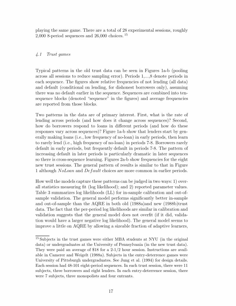
playing the same game. There are a total of 28 experimental sessions, roughly2,000 8-period sequences and 26,000 choices. 15

4.1 Trust games

Typical patterns in the old trust data can be seen in Figures 1a-b (poolingacross all sessions to reduce sampling error). Periods 1,...,8 denote periods ineach sequence. The figures show relative frequencies of not lending (all data)and default (conditional on lending, for dishonest borrowers only), assumingthere was no default earlier in the sequence. Sequences are combined into ten-sequence blocks (denoted “sequence” in the figures) and average frequenciesare reported from those blocks.

Two patterns in the data are of primary interest. First, what is the rate oflending across periods (and how does it change across sequences)? Second,how do borrowers respond to loans in different periods (and how do theseresponses vary across sequences)? Figure 1a-b show that lenders start by gen-erally making loans (i.e., low frequency of no-loan) in early periods, then learnto rarely lend (i.e., high frequency of no-loan) in periods 7-8. Borrowers rarelydefault in early periods, but frequently default in periods 7-8. The pattern ofincreasing default in later periods is particularly dramatic in later sequencesso there is cross-sequence learning. Figures 2a-b show frequencies for the eightnew trust sessions. The general pattern of results is similar to that in Figure1 although NoLoan and Default choices are more common in earlier periods.

How well the models capture these patterns can be judged in two ways: 1) over-all statistics measuring fit (log likelihood); and 2) reported parameter values.Table 3 summarizes log likelihoods (LL) for in-sample calibration and out-of-sample validation. The general model performs significantly better in-sampleand out-of-sample than the AQRE in both old (1988a)and new (1988b)trustdata. The fact that the per-period log likelihoods are similar in calibration andvalidation suggests that the general model does not overfit (if it did, valida-tion would have a larger negative log likelihood). The general model seems toimprove a little on AQRE by allowing a sizeable fraction of adaptive learners,

15 Subjects in the trust games were either MBA students at NYU (in the originaldata) or undergraduates at the University of Pennsylvania (in the new trust data).They were paid an average of $18 for a 2-1/2 hour session. Instructions are avail-able in Camerer and Weigelt (1988a). Subjects in the entry-deterrence games wereUniversity of Pittsburgh undergraduates. See Jung et al. (1994) for design details.Each session had 48-101 eight-period sequences. In each trust session, there were 11subjects, three borrowers and eight lenders. In each entry-deterrence session, therewere 7 subjects, three monopolists and four entrants.

17

which AQRE does not. 16

Table 4 gives estimated parameter values. 17 The estimated percentages ofsophisticated lenders αL are 43% and 63%, respectively, for old and new trustdata. The corresponding percentages of sophisticated borrowers are 100% and95% for old and new trust data, suggesting that virtually all the long-runborrowers are teaching.

4.2 Entry-deterrence games

Now we turn to the Jung et al. data on entry-deterrence. Since they ranexperiments both with inexperienced subjects and experienced subjects, wecan see whether subjects grow more sophisticated when they repeat an entireexperimental session.

Equilibrium predicts rates of entry and sharing to start low and rise as theend of a sequence draws near. Actual entry and sharing by inexperiencedsubjects are far too frequent in early periods but there is some convergencetoward early entry-deterrence across the experimental session (see Figures 3a-b). Inexperienced entrants just didn’t quite figure out how much it pays tofight entry in early periods.

Figures 4a-b show data from experienced subjects. The correspondence ofbehavior to equilibrium is much more dramatic. In the first sequence block,players often enter in the first 3 periods, but they quickly learn early entry israrely met with sharing, and they stay out in early periods of later sequences.

16 Note also that the model is almost as accurate when all sessions are pooled,with common parameters, as when fit statistics from session-specific estimation aretotaled up, although 40 fewer parameters are estimated when data are pooled. (Seeour 2004 working paper for details of session-by-session estimation). This is a bighint that the parameter estimates are quite stable across sessions for the teachingmodel. Our earlier working paper reports two other comparisons. Allowing φ, δ, andκ to be free parameters (common within each data set) and estimating them, ratherthan deriving them from functions as self-tuning EWA does, improves out-of-sampleaccuracy slightly in hit rate and likelihood in most data sets. Fixing the homemadeprior θ to zero hurts the likelihood substantially in two data sets and gives hit ratesless than chance (below 50%) except in the inexperienced entry game data.17 Keep in mind that in self-tuning EWA φ, δ and κ are not estimated, they are func-tions of the data. The averaged functional values of φ, δ and κ are quite consistentacross sessions. They are also in the ballpark of the values estimated in parametricEWA (see Ho et al. (2004)), except that the functional φ is always too high (.76-.77compared to unconstrained estimates of .45 and .25). The fact that pooling acrosssessions degrades overall fit only a little, and parameters are consistent across thenew and old trust data sets, is encouraging. See our working paper for details.

18

Summary statistics in Table 3 shows that the general teaching and AQREmodels are about equally accurate for experienced subjects. With 100% ofthe borrowers and lenders sophisticated (αL = αB = 1), the general modelreduces to AQRE. For inexperienced subjects, the general model is much moreaccurate than AQRE, reflecting the presence of adaptive lenders.

Table 4 shows estimated parameter values. The estimated fractions of sophis-ticated players are smaller for inexperienced subjects (αL = .67, αB = .91)than for experienced subjects (αL = αB = 1). This increase in sophisticationis also observed by Stahl (1999) in matrix games, Camerer et al. (2002) in adominance-solvable (p-beauty contest) game, and Cooper and Kagel (2001) insignaling games. This seems to be a robust finding, and a sensible one– playerscome to realize how others are learning after they play the same game in twoconsecutive sessions.

A challenging test for both the general and AQRE models is whether sim-ilar parameter values can be used to explain behavior in trust games andentry-deterrence games. These games are opposite in incentive structure in thesense that special type behavior (repaying or fighting) is mutually-beneficialin trust games but only privately-beneficial in entry-deterrence. If the samegeneral model structure and parameters can explain both games that showssome robustness which encourages broader application. In fact, the trust andinexperienced entry data give similar values of self-tuning EWA parameters ofφ (.76-.78) and δ (.15-.19). This is an encouraging first step towards a generallearning-based theory of different repeated games.

Many results are consistent across both games. The AQRE model predictsrather well, but it is helped substantially by allowing the constrained home-made prior above zero. Restricting θ = 0 degrades fit of AQRE a lot. In termsof overall out-of-sample fit, the general model is always a little better thanAQRE. The key difference between the two models is that some lenders andentrants learn in the general model but they always anticipate what borrowersand incumbents will do in AQRE. The fact that the general model generallyfits and predicts better than AQRE means that weakening sophistication of‘short-run’ players has some is empirical value. However, the two models areequivalent with experienced entry-game subjects, which shows the power ofexperimental experience to create full sophistication.

5 Model Robustness

We subject the general model to a stress test by checking the robustness of themodel using simulation (c.f. Cooper, Garvin, and Kagel (1997)). The idea ofthis robustness check is: 1) to verify if the general model is able to reproduce

19

the empirical trends exhibited by the data and 2) to assess the impact of thefeatures of the model in tracking data.

Four trends in the data emerge from the visual inspection of the figures 1-4. There are two cross-round trends: 1. the frequency of NoLoan or Entryincreases across rounds; and 2. the frequency of Default or Share increasesacross rounds. The other two are cross-sequence trends: 3. the frequency ofNoLoan or Entry decreases across sequence in early rounds but increasesacross sequence in later rounds; and 4. the frequency of Default or Share de-creases across sequences in early rounds but increases across sequences in laterrounds. We check for the statistical significance of these visual observations.

To confirm the significance of cross-round trends in the data, we run thefollowing regressions on each of the four datasets across round t:

Probkt (No Loan/Entry) = aLt + bLt · t, (17)

Probkt (Default/Sharing Given Loan/Entry) = aBt + bBt · t, (18)

where t indexes round and k indexes the sequence blocks in Figures 1-4. BothbLt and bBt are significantly positive, confirming our visual observation oftrends 1 and 2.

To check the significance of cross-sequence trends in the data, we partition eachdataset into the first 4 rounds and last 4 rounds and run separate regressionsfor each partition across sequences k:

Probkt (No Loan/Entry) = aLkR + bLkR · k, (19)

Probkt (Default/Sharing Given Loan/Entry) = aBkR + bBkR · k (20)

where R = 1 represent the first 4 rounds and R = 2 represent the last 4rounds.

We expect bLk1 < 0 and bLk2 > 0 for a significant trend 3 and bBk1 < 0 andbBk2 > 0 for a significant trend 4. We are only able to find partial confir-mation of the cross-sequence trends. Specifically, we find strong evidence ofcross-sequence trend in lender’s behavior for both the Trust data and the inex-perienced entry data in the first 4 rounds of the game (bLk1 < 0). We also findstrong evidence of cross sequence trend in incumbent’s behavior in the first 4rounds of the game (bBk1 < 0). But the second-half cross-sequence coefficientsbLk2 and bBk2 are not significant.

Next, we investigate if these significant trends in the data are replicated bythe model prediction. We first generate the prediction of the general modelby simulating choices using the parameter estimates of the general modelfrom Table 4. For each 8-round sequence, we produce 1000 simulated choice

20

paths of both lenders (or entrants) and borrowers (or incumbents). The 1000simulated paths are averaged to produce the simulated probabilities for eachsequence. These simulated probabilities are subjected to the same significancetests across periods and sequences we run for the data; slope coefficients forcross-round and cross-sequence trends for data and the simulated model arereported below the figures. The results for the Trust data and the inexperi-enced entry data are presented in Figures 5 and 6. 18 Judging from the plotsand the significant estimates, the general model is able to reproduce the sig-nificant trends in the data fairly accurately (although the estimated b. trendcoefficients are a little smaller in magnitude).

Is each key feature of the model necessary to capture the trends? We findout by “disabling” each feature individually and simulating choice using therestricted models with each feature disabled separately. There are four keyfeatures of the model: cross-sequence learning, the proportion of sophisticatedlenders, the home-made prior, and the proportion of sophisticated borrowers.The first two are parameters driving the lender’s choices and the last twoare driving the borrower’s choices. The details of the simulation and the trendsignificance regression analysis are the same as before. The plots and regressionresults are reported in Figures 7 and 8. The figures combine all sequences soseveral parameter configurations can be put on a single 3-D graph. The generalfindings benchmarked against data are:

(1) disabling cross-sequence learning results in less Loan initially and moreLoan in later rounds (the cross-round trend has a lower slope bLt andhigher intercept aLt than the general model). There is obviously morelearning in the data than within-sequence learning. We also see moredefault in later rounds in response to this lender behavior (I.e., the slopebBt when τ = 0 is lower than in the general model). In entry game, thereis more entry and less sharing in later rounds (i.e., the slope bBt whenτ = 0 is lower than the general model).

(2) disabling sophisticated lenders (αL = 0) results in a flatter rise inNoLoanfrequency across rounds (i.e., bLt with αL = 0 is lower than the generalmodel) and a steep drop in entry rate across rounds (which is goingagainst data trend). The restricted model predicts a lower default andmore sharing pattern than the data. This shows that allowing no sophis-ticated lenders harms fit.

(3) disabling the sophisticated borrowers (αB = 0) results in a flat defaultand sharing rate. This suggests that there are non-myopic borrowers. It

18 In addition, the significant cross-round effects for Camerer and Weigelt (1988b)are bLt = 0.08, bBt = 0.06 for data and bLt = 0.05, bBt = 0.04 for the model. Thesignificant cross-round effects for the experienced subjects in Jung et al. (1994) arebLt = 0.09, bBt = 0.11 for data and bLt = 0.07, bBt = 0.07 for the model. All aresignificant at 5%.

21

predicts a flatter rise in no loan across rounds than the data (bLt is toolow).

(4) disabling the home-made prior (θ = 0) results in substantially overpre-diction of default and sharing rate (They are higher than both the dataand the general model prediction in every round, i.e. aBt is higher.). Thisprovide strong evidence of the Special home-made type. It results in aflatter rise in no loan rate (bLt is lower) and an almost flat entry rate.

In general, disabling each of these four features, one at a time, shows thateach of the features contribute to the ability of the general model to describesubjects’ behavior. The simulations also indicate that each feature indeedcaptures the right part of the behavior that feature is meant to capture.

6 Conclusion

Many empirical learning models implicitly assume that players do not realizeothers are learning. This paper adds “sophisticated” players who do realizeothers are learning, in repeated games with incomplete information. Sophisti-cated players who know they are playing a repeated game have an incentiveto take actions which are costly in the short-run, but which “teach” learnerswhat to expect, in a way that benefits the teachers. Including teaching effectsextends learning models to the many domains in which economic relationshipsare long-lasting.

This paper applies a precise model of sophisticated teaching to finitely-repeatedexperimental games of trust and entry-deterrence, with incomplete informa-tion about players types (some are induced to be honest or to fight entry). Ear-lier experiments have shown that some features of behavior in these games areapproximated by very complex and delicate equilibria (Camerer and Weigelt(1988a), Jung et al. (1994)). But it is unlikely that players approximate theequilibria by introspection, and their comparative static predictions are oftenwrong (Neral and Ochs (1992)). A boundedly rational model of learning is oneanswer to the question of how people can approximate hyperrational Bayesianequilibria.

By including several learning types, the model both adds sophistication toadaptive learning, and adds learning to an AQRE model. Lenders and en-trants either learn adaptively (using a self-tuning functional EWA rule) orsophisticatedly anticipate what borrowers and incumbents will do. Borrowersand incumbents are either myopic, always behave in a special way (trustworthyor fighting entry), or teach strategically.

A key difference between the proposed model and equilibrium is that the play-

22

ers build reputations in AQRE (“this guys seems honest”), but the learners’strategies have reputations (“entry is dangerous”) in the proposed model. Theproposed model is also a partial equilibrium one, because some adaptive play-ers do not fully anticipate what others will do.

The general model was fit to 28 sessions of data from both repeated trust andentry games. Both models reproduce most of the basic trends in the data, par-ticularly increasing default and market-sharing in later periods of a sequence,and some cross-sequence learning. The key parameter in the general model isthe fraction of strategic teachers, αB . This figure is reliably estimated to beabout .91 for inexperienced entry-game subjects and close to 1 for trust gamesand experienced entry-game data. The fact that αB rises with subject expe-rience corroborates other findings. The AQRE model generally fits reliablyworse than the general model, which is an indication that adding a learningcomponent to equilibrium models helps explain how people behave.

A key point is that the same model can account for quite different behaviorin these games: Borrowers in trust games behave in an honest way that ismutually-beneficial, while aggressive incumbents benefit only themselves. Thesame model explains both because the two behaviors emerge endogenouslyfrom the same kind of interaction between teaching and payoffs.

Finally, we subject the general model to a stress test to check the modelrobustness. Relying only on parameter estimates, the general model is ableto simulate behaviors that match the significant trends found in the data.Furthermore, we show that this descriptive ability degrades significantly whenany of the four key features of the model is turned off.

In future research, it would be useful to endogenize some of the parametersof most interest (particularly the rate of sophistication αB). The model couldalso be applied to games and markets where the interaction of sophisticationand adaptive learning is interesting (e.g. inflation-setting, see Sargent (1999);and price bubbles, see Smith, Suchanek, and Williams (1988), Camerer andWeigelt (1990) and Lei, Noussair, and Plott (2001)).

References

Andreoni, J., Miller, J., 1993. Rational cooperation in the finitely repeatedprisoner’s dilemma: Experimental evidence. Economic Journal 103, 570–585.

Cachon, G. P., Camerer, C. F., 1996. Loss-avoidance and forward inductionin experimental coordination games. Quarterly Journal of Economics 111,165–194.

23

Camerer, C. F., 2003. Behavioral Game Theory: Experiments on StrategicInteraction, 1st Edition. Princeton University Press, Princeton, N.J.

Camerer, C. F., Ho, T.-H., 1999. Experience-weighted attraction learning innormal-form games. Econometrica 67, 827–874.

Camerer, C. F., Ho, T.-H., Chong, J.-K., 2002. Sophisticated EWA learn-ing and strategic teaching in repeated games. Journal of Economic Theory104 (1), 137–188.

Camerer, C. F., Weigelt, K., 1988a. Experimental tests of a sequential equi-librium reputation model. Econometrica 56, 1–36.

Camerer, C. F., Weigelt, K., 1988b. Measuring beliefs in reputation games,presentation to the Economic Science Association.

Camerer, C. F., Weigelt, K., 1990. Inducing bubble expectations in experi-mental asset markets, unpublished manuscript.

Camerer, C. F., Weigelt, K., 2005. Belief calibration, QRE and learning inrepeated trust games. In: Lupia, A., Alt, J. (Eds.), Essays in Honor ofRichard McKelvey.

Cooper, D., Kagel, J., 2001. Learning and transfer in signaling games, workingPaper, Department of Economics, Case Western Reserve University.

Cooper, D. J., Garvin, S., Kagel, J. H., 1997. Signalling and adaptive learningin an entry limit pricing game. RAND Journal of Economics 28 (4), 662–683.

Fehr, E., Gachter, S., 2000. Fairness and retaliation: The economics of reci-procity. Journal of Economic Perspective 14, 159–181.

Fudenberg, D., Kreps, D., 1990. A theory of learning, experimentation andequilibrium in games, working Paper, Stanford University.

Fudenberg, D., Levine, D., 1989. Reputation and equilibrium selection ingames with a patient player. Econometrica 57, 759–778.

Goeree, J. K., Holt, C. A., 1999. Stochastic game theory: For playing games,not just for doing theory, proceedings of the National Academy of Sciences.

Ho, T.-H., Camerer, C. F., Chong, J.-K., May 2004. The economics of learningmodels: A self-tuning theory of learning in games, working Paper, Universityof California Berkeley.

Ho, T.-H., Camerer, C. F., Weigelt, K., 1998. Iterated dominance and iteratedbest-response in p-beauty contests. American Economic Review 88, 947–969.

Jung, Y. J., Kagel, J. H., Levin, D., 1994. On the existence of predatorypricing: An experimental study of reputation and entry deterrence in thechain-store game. RAND Journal of Economic 25, 72–93.

Kalai, E., Lehrer, E., 1993. Rational learning leads to nash equilibrium. Econo-metrica 61 (5), 1019–1045.

Kreps, D., 1990. Corporate culture and economic theory. In: Alt, J., Shepsle,K. (Eds.), Perspectives on Positive Political Economy. Cambridge UniversityPress, Cambridge.

Kreps, D., Wilson, R., 1982. Reputation and imperfect information. Journalof Economic Theory 27 (1), 253–279.

Lei, V., Noussair, C., Plott, C., 2001. Nonspeculative bubbles in experimentalasset markets: Lack of common knowledge of rationality vs. actual irra-

24

tionality. Econometrica 69 (4), 831–859.McKelvey, R. D., Palfrey, T. R., 1992. An experimental study of the centipedegame. Econometrica 60, 803–836.

McKelvey, R. D., Palfrey, T. R., 1998. Quantal response equilibria for extensiveform games. Experimental Economics 1, 9–41.

Milgrom, P., Roberts, J., 1991. Adaptive and sophisticated learning in re-peated normal form games. Games and Economic Behavior 3, 82–100.

Mookherjee, D., Sopher, B., 1994. Learning behavior in an experimentalmatching pennies game. Games and Economic Behavior 7, 62–91.

Neral, J., Ochs, J., 1992. The sequential equilibrium theory of reputation build-ing: A further test. Econometrica 60, 1151–1169.

Palfrey, T. R., Rosenthal, H., 1988. Private incentives in social dilemmas: Theeffects of incomplete information and altruism. Journal of Public Economics35, 309–332.

Partow, Z., Schotter, A., 1993. Does game theory predict well for the wrongreasons? an experimental investigation, working Paper 93-46, C.V. StarrCenter for Applied Economics, New York University.

Sargent, T., 1999. The Conquest of American Inflation, 1st Edition. PrincetonUniversity Press, Princeton.

Selten, R., 1991. Anticipatory learning in 2-person games. In: Selten, R. (Ed.),Game Equilibrium Models. Vol. I. Springer-Verlag, Berlin, pp. 98–154.

Selten, R., Stoecker, R., 1986. End behavior in sequences of finite prisoner’sdilemma supergames: A learning theory approach. Journal of Economic Be-havior and Organization 7, 47–70.

Smith, V. L., Suchanek, G., Williams, A., 1988. Bubbles, crashes and endoge-nous expectations in experimental spot asset markets. Econometrica 56,1119–1151.

Stahl, D. O., 1999. Sophisticated learning and learning sophistication, workingPaper, University of Texas at Austin.

Watson, J., 1993. A ‘reputation’ refinement without equilibrium. Economet-rica 61, 199–205.

Watson, J., Battigali, P., 1997. On ‘reputation’ refinements with heterogeneousbeliefs. Econometrica 65, 363–374.

7 Appendix: Self-tuning EWA Model Specification

Ho et al. (2004) developed a Self-tuning EWA model in which the fixed pa-rameters φ and δ are replaced by functions of data which self-adjust acrossgames and over time. These functions determine parameter values for eachplayer, each round and each sequence, which are then plugged into the EWAupdating equation to determine attractions.

The function φ(k, t) is designed to detect change in the learning environment.

25

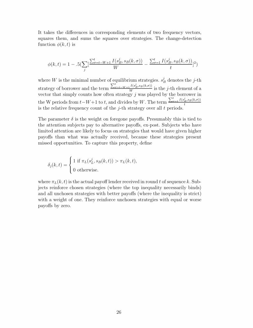
It takes the differences in corresponding elements of two frequency vectors,squares them, and sums the squares over strategies. The change-detectionfunction φ(k, t) is

φ(k, t) = 1− .5(∑j

[

∑tσ=t−W+1 I(s

jB, sB(k, σ))

W−

∑tσ=1 I(s

jB, sB(k, σ))

t]2)

where W is the minimal number of equilibrium strategies. sjB denotes the j-th

strategy of borrower and the term∑t

σ=t−W+1I(sj

B,sB(k,σ))

Wis the j-th element of a

vector that simply counts how often strategy j was played by the borrower in

the W periods from t−W+1 to t, and divides byW . The term∑t

σ=1I(sj

B,sB(k,σ))

t

is the relative frequency count of the j-th strategy over all t periods.

The parameter δ is the weight on foregone payoffs. Presumably this is tied tothe attention subjects pay to alternative payoffs, ex-post. Subjects who havelimited attention are likely to focus on strategies that would have given higherpayoffs than what was actually received, because these strategies presentmissed opportunities. To capture this property, define

δj(k, t) =

1 if πL(s

jL, sB(k, t)) > πL(k, t),

0 otherwise.

where πL(k, t) is the actual payoff lender received in round t of sequence k. Sub-jects reinforce chosen strategies (where the top inequality necessarily binds)and all unchosen strategies with better payoffs (where the inequality is strict)with a weight of one. They reinforce unchosen strategies with equal or worsepayoffs by zero.

26

Short-Run Player (e.g., Lenders, Entrants)

Proportion Specification of Behavior

Long-Run Player (e.g., Borrowers, Incumbents)

Proportion Specification of Behavior

Adaptive 1-αL Section 2.1 Special (Induced) (e.g., Honest. Aggressive)

p Section 2.3

Sophisticated αL Section 2.2 Normal (Induced)

(Dishonest, Non-aggressive) 1-p

Special (Home-made) θ Section 2.3 Normal 1− θ Myopic 1-αΒ Section 2.4 Sophisticated αΒ Section 2.5

Table 1: A Model of Repeated Games with both Adaptive and Sophisticated Players

Table 2: Payoffs for the Borrower-lender Trust Games and the Entry-deterrence Games

Payoffs in the borrower-lender trust game, Camerer and Weigelt [1988a]

lender borrower payoffs to payoffs to borrower

strategy strategy lender normal (X) honest (Y)

loan default −100∗ 150 0

repay 40 60 60

no loan no choice 10 10 10

Payoffs in the entry-deterrence game, Jung, Kagel and Levin [1994]

entrant incumbent payoffs to payoffs to incumbent

strategy strategy entrant normal (X) fighter (Y)

in fight 80 70 160

share 150 160 70

out no choice 95 300 300

Note: ∗ Loan-default lender payoffs were -50 in sessions 6-8 and -75 in sessions 9-10.

Table 3: In-sample and Out-of-sample Performance of the General Model and AQRE Model

Dataset Camerer and Camerer andWeigelt (1988a) Weigelt (1988b) Inexperienced Experienced

Subjects Subjects

In-sample Calibration 1

Sample size 5757 3820 5847 2232

Log-likelihoodThe General Model -2919.43 -2007.20 -2246.97 -1345.76AQRE -3218.52 -2094.17 -2418.43 -1345.76

Log-likelihood Ratio 2 598.18 173.93 342.91 0.00

Average ProbabilityThe General Model 0.60 0.59 0.68 0.55AQRE 0.57 0.58 0.66 0.55

Out-of-sample Validation

Sample size 2894 1882 2866 1072

Log-likelihoodThe General Model -1425.16 -947.25 -1341.15 -553.11AQRE -1525.69 -989.44 -1425.53 -553.11

Average ProbabilityThe General Model 0.61 0.60 0.63 0.60AQRE 0.59 0.59 0.61 0.60

Note 1: Calibrated on all observations for 70% of the subjects instead of 70% observations of all subjects.

Note 2: Threshold for significant χ2 test is 12.59 at 5% for 6 degrees of freedom

Jung, Kagel and Levin (1994)

Table 4: Parameter Estimates 1

Dataset Camerer and Camerer andWeigelt (1988a) Weigelt (1988b) Inexperienced Experienced

Subjects Subjects

The General Model

Adaptive LenderFunctional φ 0.76 0.77 0.78 0.76Functional δ 0.15 0.16 0.19 0.34

τ 0.94 0.68 0.35 0.12A0 (No Loan/Not Enter) -2.09 -1.52 -1.63 0.39

λaL 11.40 5.89 3.90 3.70

Sophisticated LenderαL 0.43 0.63 0.67 1.00

λsL 7.75 8.19 5.41 6.53

Myopic Borrowerλm

B 2.66 3.76 5.62 3.10

Sophisticated BorrowerαB 1.00 0.95 0.91 1.00

λsB 5.87 8.45 2.90 1.36

θ 0.28 0.28 0.18 0.17

Honest Borrowerλh

B 27.32 24.76 5.70 6.30

Agent-based Quantal Response Equilibrium (AQRE)

Sophisticated LenderαL 1.00 1.00 1.00 1.00

λsL 6.31 5.37 4.76 6.53

Sophisticated BorrowerαB 1.00 1.00 1.00 1.00

λsB 3.84 4.76 3.28 1.36

θ 0.27 0.28 0.16 0.17

Honest Borrowerλh

B 26.70 25.89 2.75 6.30

Note 1: All sessions in a dataset are pooled to produce a common set of estimates except for the scale parameterslike the λs which are session-specific. The estimates reported here are averages. Standard errors are reported in

our working paper.

Jung, Kagel and Levin (1994)

Figures 1a-b: Frequency Plots for the Trust Data from Camerer and Weigelt [1988a]

Figures 2a-b: Frequency Plots for the Unpublished Trust Data from Camerer and Weigelt [1988b]

12

34

56

78

1 2 3 45

67

8

00.10.20.30.4

0.5

0.6

0.7

0.8

0.9

1

Freq

RoundSequence

Figure 1a: Empirical Frequency for No Loan

12

34

56

78

1 2 3 4 56

78

-0.10

0.10.20.30.40.50.60.70.80.9

1

Freq

RoundSequence

Figure 1b: Empirical Frequency for Default conditional on Loan (Dishonest Borrower)

12

34

56

78

1 2 3 45

67

8

00.10.20.30.4

0.5

0.6

0.7

0.8

0.9

1

Freq

RoundSequence

Figure 2a: Empirical Frequency for No Loan

12

34

56

78

1 2 3 4 56

78

-0.10

0.10.20.30.40.50.60.70.80.9

1

Freq

RoundSequence

Figure 2b: Empirical Frequency for Default conditional on Loan (Dishonest Borrower)

Figures 3a-b: Frequency Plots on Inexperienced Subjects from the Entry Data from Jung, Kagel and Levin [1994]

Figures 4a-b: Frequency Plots on Experienced Subjects from the Entry Data from Jung, Kagel and Levin [1994]

12

34

56

78

1 2 3 45

67

8

00.10.20.30.4

0.5

0.6

0.7

0.8

0.9

1

Freq

RoundSequence

Figure 3a: Empirical Frequency for Entry

12

34

56

78

1 2 3 4 56

78

-0.10

0.10.20.30.40.50.60.70.80.9

1

Freq

RoundSequence

Figure 3b: Empirical Frequency for Sharing conditional on Entry (Weak Incumbent)

12

34

56

78

1 2 3 45

67

8

00.10.20.30.4

0.5

0.6

0.7

0.8

0.9

1

Freq

RoundSequence

Figure 4a: Empirical Frequency for Entry

12

34

56

78

1 2 3 4 56

78

-0.10

0.10.20.30.40.50.60.70.80.9

1

Freq

RoundSequence

Figure 4b: Empirical Frequency for Sharing conditional on Entry (Weak Incumbent)

Figures 5a-d: Cross-sequence and Cross-round Effects for the Trust Data from Camerer and Weigelt [1988a]

Cross-sequence Trends: bLk1 (data) = -0.02, bLk1 (model) = -0.01. Both are significant at 5%

Cross-round Trends: bLt (data) = 0.10, bLt (model) = 0.05, bBt (data) = 0.10, bBt (model) = 0.04. All are significant at 5%

12

34

56

78

1 2 3 4 5 67

8

00.10.20.30.40.50.60.70.80.9

1

Freq

RoundSequence

Figure 5a: The General Model Simulated Frequency for No Loan

12

34

56

78

1 2 3 4 5 67

8

-0.10

0.10.20.30.40.50.60.70.80.9

1

Freq

RoundSequence

Figure 5b: The General Model Simulated Frequency for Default conditional on Loan (Dishonest Borrower)

Figures 6a-b: Cross-sequence and Cross-round Effects for Inexperienced Subjects from the Entry Data from Jung, Kagel and Levin [1994]

Cross-sequence Trends: bLk1 (data) = -0.02, bLk1 (model) = -0.01, bBk1 (data) = -0.03, bBk1 (model) = -0.01. All are significant at 5%

Cross-round Trends: bBt (data) = 0.05, bBt (model) = 0.04. All are significant at 5%

12

34

56

78

1 2 3 4 5 67

8

00.10.20.30.40.50.60.70.80.9

1

Freq

RoundSequence

Figure 6a: The General Model Simulated Frequency for Entry

12

34

56

78

1 2 3 4 5 67

8

-0.10

0.10.20.30.40.50.60.70.80.9

1

Freq

RoundSequence

Figure 6b: The General Model Simulated Frequency for Sharing conditional on Entry (Weak Incumbent)

Incumbent: bBt (data) = 0.05, bBt (model) = 0.04, bBt (ττττ=0) = 0.03, bBt (ααααL=0) = 0.03, bBt (ααααB=0) = 0.00, bBt (θθθθ=0) = 0.03

Figures 8a-b: Parameter Restrictions for Inexperienced Subjects from the Entry Data from Jung, Kagel and Levin [1994]

Figures 7a-b: Parameter Restrictions for the Trust Data from Camerer and Weigelt [1988a]

Lender: bLt (data) = 0.10, bLt (model) = 0.05, bLt (ττττ=0) = 0.03, bLt (ααααL=0) = 0.04, bLt (ααααB=0) = 0.04, bLt (θθθθ=0) = 0.04. Borrower: bBt (data) = 0.10, bBt (model) = 0.04, bBt (ττττ=0) = 0.03, bBt (ααααL=0) = 0.04, bBt (ααααB=0) = 0.00, bBt (θθθθ=0) = 0.05

12

34

56

78

Dat

aG

ener

alta

u=0

alph

aL=0

alph

aB=0

thet

a=0

00.10.20.30.40.50.60.70.80.91

Prob

Round

Model

Figure 8a: Average Probability of Entry

12

34

56

78

Dat

aG

ener

alta

u=0

alph

aL=0

alph

aB=0

thet

a=0

00.10.20.30.40.50.60.70.80.91

Prob

Round

Model

Figure 8b: Average Probability of Sharing Given Entry (WeakIncumbent)

12

34

56

78

Dat

aG

ener

alta

u=0

alph

aL=0

alph

aB=0

thet

a=0

00.10.2

0.3

0.4

0.5

0.6

0.7

0.8

Prob

RoundModel

Figure 7a: Average Probability of No Loan

12

34

56

78

Dat

aG

ener

alta

u=0

alph

aL=0

alph

aB=0

thet

a=0

00.10.20.30.40.50.60.70.80.9

Prob

RoundModel

Figure 7b: Average Probability of Default Given Loan (DishonestBorrower)