Technische Universität Wien A-1040 Wien � Karlsplatz 13 � Tel. +43-1-58801-0 � www.tuwien.ac.at

A Layered Particle-Based Fluid Model for Real-Time Rendering of

Water

DIPLOMARBEIT

zur Erlangung des akademischen Grades

Diplom-Ingenieur

im Rahmen des Studiums

Computergraphik/Digitale Bildverarbeitung

eingereicht von

Florian Bagar Matrikelnummer 0500041

an der Fakultät für Informatik der Technischen Universität Wien Betreuung Betreuer: Associate Prof. Dipl.-Ing. Dipl.-Ing. Dr.techn. Michael Wimmer Mitwirkung: Dipl.-Ing. Mag.rer.soc.oec. Dr.techn. Daniel Scherzer Wien, 28.09.2010

(Unterschrift Verfasser/in) (Unterschrift Betreuer/in)

Erklarung zur Verfassung der Arbeit

Florian BagarSchonbrunnerstraße 29/A381050 Wien

”Hiermit erklare ich, dass ich diese Arbeit selbstandig verfasst habe, dass ichdie verwendeten Quellen und Hilfsmittel vollstandig angegeben habe und dassich die Stellen der Arbeit - einschließlich Tabellen, Karten und Abbildungen-, die anderen Werken oder dem Internet im Wortlaut oder dem Sinn nachentnommen sind, auf jeden Fall unter Angabe der Quelle als Entlehnungkenntlich gemacht habe.”

Ort, Datum:Unterschrift:

Abstract

We present a physically based real-time water simulation and renderingmethod that brings volumetric foam to the real-time domain, significantlyincreasing the realism of dynamic fluids. We do this by combining a particle-based fluid model that is capable of accounting for the formation of foamwith a layered rendering approach that is able to account for the volumetricproperties of water and foam. Foam formation is simulated through Webernumber thresholding. For rendering, we approximate the resulting water andfoam volumes by storing their respective boundary surfaces in depth maps.This allows us to calculate the attenuation of light rays that pass throughthese volumes very efficiently. We also introduce an adaptive curvature flowfilter that produces consistent fluid surfaces from particles independent ofthe viewing distance.

Kurzfassung

Wir prasentieren ein physikalisch basiertes Echtzeit-Wassersimulations- undRenderingverfahren, welches volumetrischen Schaum in den Echtzeitbere-ich einfuhrt und den Realismus von dynamischen Flussigkeiten maßgeblichverbessert. Dazu kombinieren wir ein partikelbasiertes Flussigkeitsmodell,welches das Entstehen von Schaum berucksichtigt. Der Ansatz dieses Modellsist auf drei Schichten aufgebaut und bezieht die volumetrischen Eigenschaftenvon Wasser und Schaum ein. Die Bildung von Schaum basiert auf der so-genannten

”Weber-Nummer“, wobei die Schaumbildung ab einem gewissen

Schwellwert einsetzt. Die Wasser- und Schaumoberflache wird durch Tiefen-bilder reprasentiert auf deren Grundlage die jeweilige Dicke der Schichtenberechnet wird, was wiederum eine effiziente Berechnung der optischen Eigen-schaften des Wassers zulasst. Des Weiteren fuhren wir das sogenannte Adap-tive Curvature Flow Filtering ein. Es ermoglicht uns eine Wasseroberflachezu generieren, die, unabhangig vom Betrachtungsabstand, immer gleich vielDetail aufweist.

Contents

1. Introduction . . . . . . . . . . . . . . . . . . . . . . . . . . . . . . 81.1 Scope of the work . . . . . . . . . . . . . . . . . . . . . . . . . 81.2 Motivation . . . . . . . . . . . . . . . . . . . . . . . . . . . . . 91.3 Main Contributions . . . . . . . . . . . . . . . . . . . . . . . . 101.4 Thesis Structure . . . . . . . . . . . . . . . . . . . . . . . . . . 11

2. Previous Work . . . . . . . . . . . . . . . . . . . . . . . . . . . . . 132.1 Fluid Simulation . . . . . . . . . . . . . . . . . . . . . . . . . 132.2 Fluid Rendering . . . . . . . . . . . . . . . . . . . . . . . . . . 142.3 Smoothed Particle Hydrodynamics . . . . . . . . . . . . . . . 152.4 Offline Methods . . . . . . . . . . . . . . . . . . . . . . . . . . 17

2.4.1 Two-Way Coupled SPH and Particle Level Set FluidSimulation . . . . . . . . . . . . . . . . . . . . . . . . . 17

2.4.2 Simulation of Two-Phase Flow with Sub-Scale Dropletand Bubble Effects . . . . . . . . . . . . . . . . . . . . 19

2.4.3 Realistic Animation of Fluid with Splash and Foam . . 192.4.4 Bubbling and Frothing Liquids . . . . . . . . . . . . . 21

2.5 Real-Time Methods . . . . . . . . . . . . . . . . . . . . . . . . 222.5.1 Real-Time Simulations of Bubbles and Foam within a

Shallow Water Framework . . . . . . . . . . . . . . . . 222.5.2 Screen Space Meshes . . . . . . . . . . . . . . . . . . . 232.5.3 Screen Space Fluid Rendering with Curvature Flow . . 25

2.6 APIs . . . . . . . . . . . . . . . . . . . . . . . . . . . . . . . . 302.6.1 OpenGL . . . . . . . . . . . . . . . . . . . . . . . . . . 302.6.2 Shader Authoring Language . . . . . . . . . . . . . . . 30

3. Method . . . . . . . . . . . . . . . . . . . . . . . . . . . . . . . . . 323.1 Adaptive Curvature Flow . . . . . . . . . . . . . . . . . . . . 343.2 Real-Time Foam . . . . . . . . . . . . . . . . . . . . . . . . . 35

3.2.1 Foam Formation . . . . . . . . . . . . . . . . . . . . . 363.2.2 Layer Creation . . . . . . . . . . . . . . . . . . . . . . 363.2.3 Layer Compositing . . . . . . . . . . . . . . . . . . . . 40

Contents 6

4. Implementation . . . . . . . . . . . . . . . . . . . . . . . . . . . . 414.1 Textures and Render Targets . . . . . . . . . . . . . . . . . . 434.2 Simulation Update . . . . . . . . . . . . . . . . . . . . . . . . 454.3 View Frustum Culling . . . . . . . . . . . . . . . . . . . . . . 464.4 Main Scene Rendering . . . . . . . . . . . . . . . . . . . . . . 484.5 Point Sprites . . . . . . . . . . . . . . . . . . . . . . . . . . . 494.6 Depth Passes . . . . . . . . . . . . . . . . . . . . . . . . . . . 50

4.6.1 Water Depth . . . . . . . . . . . . . . . . . . . . . . . 504.6.2 Foam Depth . . . . . . . . . . . . . . . . . . . . . . . . 51

4.7 Adaptive Curvature Flow Filtering . . . . . . . . . . . . . . . 524.8 Layer Thicknesses . . . . . . . . . . . . . . . . . . . . . . . . . 56

4.8.1 Water Layer . . . . . . . . . . . . . . . . . . . . . . . . 574.8.2 Foam Layer . . . . . . . . . . . . . . . . . . . . . . . . 58

4.9 Water Rendering including Foam . . . . . . . . . . . . . . . . 614.9.1 Helper Functions . . . . . . . . . . . . . . . . . . . . . 624.9.2 Back to Front Compositing . . . . . . . . . . . . . . . 624.9.3 Compositing Shader . . . . . . . . . . . . . . . . . . . 644.9.4 Shadowing . . . . . . . . . . . . . . . . . . . . . . . . . 664.9.5 Spray Particles . . . . . . . . . . . . . . . . . . . . . . 66

5. Results . . . . . . . . . . . . . . . . . . . . . . . . . . . . . . . . . 685.1 Scenes . . . . . . . . . . . . . . . . . . . . . . . . . . . . . . . 685.2 Performance . . . . . . . . . . . . . . . . . . . . . . . . . . . . 735.3 Limitations . . . . . . . . . . . . . . . . . . . . . . . . . . . . 75

6. Summary and future work . . . . . . . . . . . . . . . . . . . . . . 776.1 Conclusion . . . . . . . . . . . . . . . . . . . . . . . . . . . . . 776.2 Future Work . . . . . . . . . . . . . . . . . . . . . . . . . . . . 79

A. Shader Code . . . . . . . . . . . . . . . . . . . . . . . . . . . . . . 80A.1 General . . . . . . . . . . . . . . . . . . . . . . . . . . . . . . 80A.2 Depth Passes . . . . . . . . . . . . . . . . . . . . . . . . . . . 85A.3 Adaptive Curvature Flow . . . . . . . . . . . . . . . . . . . . 88A.4 Layer Thicknesses . . . . . . . . . . . . . . . . . . . . . . . . . 91A.5 Compositing . . . . . . . . . . . . . . . . . . . . . . . . . . . . 93

List of Figures . . . . . . . . . . . . . . . . . . . . . . . . . . . . . . . 99

List of Tables . . . . . . . . . . . . . . . . . . . . . . . . . . . . . . . 101

List of Listings . . . . . . . . . . . . . . . . . . . . . . . . . . . . . . . 102

Contents 7

Bibliography . . . . . . . . . . . . . . . . . . . . . . . . . . . . . . . . 104

Acknowledgements . . . . . . . . . . . . . . . . . . . . . . . . . . . . 109

Chapter 1

Introduction

Over the last decade, simulation and rendering of complex natural phenom-ena such as fire, smoke, cloud or fluid has been an active and one of the mostimportant research areas in computer graphics. Among these phenomena,water may be the most fascinating and challenging problem. Fluids suchas water are an essential substance in our daily life and have attracted theattention of many researchers. Although the visual quality has improved,the lack of realism still offers a lot of room for improvement.

1.1 Scope of the work

Under the assumption that a fluid is at rest, it can be represented as a flatsurfaces. For instance, this representation has been used to realistically ren-der ocean scenes in computer games. This is a reasonable assumption inthe field of games, but not sufficient for computer generated films or motionpictures (and even in modern computer games one would prefer a more ad-vanced method). Because as the realism of a scene increases, also the fluidhas to be simulated and rendered in a more realistic way. The problem isthat a fluid can move in a very complex way and even topologically changescan occur if the fluid is separated because of turbulent motion. Furthermore,the visual appearance of a fluid like water is based on complex optical effects,caused by reflection and refraction. As well as caused by caustics, which arecomplex patterns of light that can be seen on surfaces in presence of water(for instance, those formed on the floor of a swimming pool).

Real water also has additional features such as foam, bubbles and spray,appearing through advection, created by interaction with wind or formed bya water jet mixing gas with liquid. In general as proposed by Joseph [18],foam is a two-phase medium of gas and liquid with a particular structureconsiting of gas pockets trapped in a network of thin liquid films and plateauborders. Taking these features, including the optical effects, in considerationextremely enhances the realism of scenes including water. But as one can

Chapter 1. Introduction 9

imagine, due to the complexity of fluid physics the computational cost isvery high. This is especially true for offline rendering, although it achievesrealistically and detailed results.

For offline rendering the focus is very high-quality and thus it is notinteractively. For instance, objects or the view point cannot be moved by theviewer within the scene because the rendering time for a single image (referredto as frame) is too long. Also interaction with a fluid included in the sceneis not possible because of this circumstance. Contrary to offline rendering,performance has the highest priority concerning real-time rendering. Thusa real-time application is able to synthesize the frames fast enough to keepthe viewer immersed in the scene and also interaction with fluids is possible.For example, the viewer can throw objects into the fluid which float onthe fluid or sink. An application is classified as real-time if it renderes atleast 15 frames per second (fps) [1], which permits the viewer to distinguishindividual frames. In this context the increasing performance of today’sGPUs is an important factor because it enables real-time methods to achieveimproved visual quality, simulate complex physics on the GPU, and evenadapt approaches from offline rendering methods. For instance, the fluidsimulation used in this thesis is carried out on the GPU resulting in a highperformance gain compared to a CPU fluid simulation.

Simulation of fluids like water can be classified into Eulerian and La-grangian approaches. The former build on a fixed grid in space, and are anobvious choice for GPU-based calculation, since calculations on the cells ofa grid are easily parallelizable. However, these approaches are not intuitivefor flows because they limit the simulation to the space where the grid is de-fined. Lagrangian-approaches, like Smoothed Particle Hydrodynamics (SPH),simulate a fluid by moving discrete volume elements, and are therefore notrestricted concerning the simulation space. Furthermore, particle-based fluidsimulations are also suited for simulating topologically changes of water sur-faces.

The remaining part of this chapter provides a motivation, introduces areal-time fluid simulation and rendering system developed for this thesis, andshows the main contributions and the structure of this thesis.

1.2 Motivation

Dynamic fluids are a desirable element of many real-time applications. Sofar, the mathematical complexity of realistically simulating and rendering thebehavior and interaction of fluids with the environment has hindered their

Chapter 1. Introduction 10

widespread use. One promising approach would be to render the results ofSPH simulations using splatting, but the locally high curvature of sphericalsplatting primitives results in an unrealistic jelly-like appearance.

Only recently, van der Laan et al. [37] proposed curvature-based screenspace filtering for rendering the result of SPH simulations. The approach al-leviates sudden changes in curvature between the particles and creates a con-tinuous and smooth surface. While this method is a significant step towardsrealistic fluid rendering in real time, there is room for improvement. First,the screen-space curvature flow formulation is highly dependent on viewerdistance. While fluids farther away from the viewer are overly smoothed,fluids near the viewer almost completely retain the undesirable spherical par-ticle structure. Second, there exists as yet no realistic real-time method tocreate foam, which is an important visual element in most situations wherereal-time fluids are used (see Figure 1.1).

The main algorithm discussed in this thesis was also published in a paper[3] at the “21st Eurographics Symposium on Rendering”.

Fig. 1.1: A scene rendered with simple noise-based foam [37] (left) and with ournew method (right);

1.3 Main Contributions

This thesis presents a real-time fluid simulation and rendering system thatovercomes these drawbacks:

Chapter 1. Introduction 11

• We introduce an adaptive curvature flow filtering algorithm for smoothedparticle hydrodynamics rendering which accounts for perspective dueto is independence from the viewpoint and avoids over- or under-smoothing as present in previous methods. The construction of thewater surface and the filtering is not based on polygonization, and thusdoes not suffer from the associated tessellation artifacts.

• We introduce a fast physically based foam rendering approach using We-ber number thresholding and a volumetric layer-based rendering system(see Figure 3.3). Foam can appear as top-most layer or between twowater layers, as it is the case when a turbulent stream, like a waterfall,immerges into resting water with high impact. We calculate the thick-ness of each layer and perform volumetric back to front compositingalong the viewing rays. Thus, objects of the background scene becomeless visible depending on the amount of water and foam that is in frontof them.

• Our method is almost as fast as previous approaches and has compa-rable performance with the benefit of improved image quality.

• Our method is highly configurable from an artistic point of view, andthus can produce a multiplicity of visual appearances which match thebackground scene and create the desired atmosphere.

• In addition, the algorithm is simple to implement and integrate intoexisting rendering engines. Furthermore, all rendering steps are calcu-lated using shaders and intermediate render targets on the GPU.

1.4 Thesis Structure

The thesis is structured into different chapters as follows:

• Chapter 2 gives an overview about previous work. First, the chapterdescribes the smoothed particle hydrodynamics formalism. Then, re-cent offline methods are described and finally an overview of real-timeapproaches is given.

• Chapter 3 explains our method which is separated into our adaptivecurvature flow filtering, and real-time foam rendering.

Chapter 1. Introduction 12

• Chapter 4 deals with the implementation of our method. The chapterdescribes the used application programming interfaces, gives an top-level overview of the involved classes, and presents a detailed descrip-tion of the rendering algorithm.

• Chapter 5 shows results that are achieved using our simulation andrendering method and provides a detailed performance comparison.The Chapter also discusses limitations of our method.

• Chapter 6 summarizes the thesis’ contents by drawing a conclusion anddiscussing possible future enhancements.

Chapter 2

Previous Work

Several offline and real-time methods exist to simulate and render dynamicfluid flows. This chapter is a collection of some of these approaches whichare related to our work. As stated in chapter 1 the simulation of fluids cancategorized into two types, the Eulerian- and the Lagrangian- approach.

2.1 Fluid Simulation

In general, the dynamic behavior of incompressible fluids is described by theso-called Navier Stokes equations [14]. Methods based on the Eulerian ap-proach subdivide the simulation space into a regular grid. This grid is usedto simulate the fluid dynamics, and the Navier Stokes Equations are solvedby discretizing the equations, using this grid. Each cell of this grid containscertain quantities such as velocity, pressure or density needed for the simula-tion and in every simulation step these values are updated depending on theflow. The Navier Stokes equations are also suitable for simulating phenom-ena such as clouds, foam or smoke. One problem that arises by using a fixedgrid, is that small scale phenomena like foam, bubbles or spray can hardlybe tracked because too coarse grid resolutions are used. One could try torefine the grid that is being used, but the drawbacks are increased perfor-mance and memory requirements and for this reason only limited applicablefor real-time methods. Thus, many methods based on the Eulerian approachdecouple small scale effects from the main fluid simulation and offers themto simulate effects such as foam or bubbles on a much smaller scale thanthe underlying grid. This is especially the case for offline methods. Anotherdrawback is that the fluid is restricted to stay with the grid and thus cannotflow everywhere within a scene. Common methods to solve the Navier Stokesequations for the Eulerian case are finite element techniques [34].

In the Lagrangian formulation of a fluid, particles are used to completelydefine the fluid and to solve the Navier Stokes equations. Compared to theEulerian approach where the fluid is tracked at fixed position in space, in the

Chapter 2. Previous Work 14

case of the Lagrangian approach the particles move with the fluid and thustrack the fluid. Particle-based fluid simulations such as SPH which is used bythe algorithm presented in this thesis (see section 2.3) have several advantagescompared to grid-based methods. For instance, the fluid is not restricted toa fixed volume in space and even topologically changes of the fluid surfaceare handled because of their particle-based nature. Furthermore, collisiondetection with the surrounding environment and also with dynamic objectscan easily be determined because each particle carries position and velocityinformation, which are sufficient to calculate any collision. However, themajor drawback of particle-based methods is the high particle amount thatis required to simulate realistically behaving fluids. Moreover, the particlesshould be small in size to ensure that small scale effects can be treated in anappropriate way and thus the particle count has to be increased to achieverealistically results. Furthermore, it is a difficult to extract a surface forrendering.

2.2 Fluid Rendering

To achieve realistically looking renderings including optical effects such as re-flection and refraction the fluid surface has to be reconstructed. A commonmethod for surface extraction is the marching cubes [19] algorithm which isapplicable to both grid-based and particle-based methods. The algorithmextracts a polygonal mesh that approximates the iso-surface from a three-dimensional grid. The drawback with respect to particle-based methods isthat the simulation space has to be subdivided into a grid. Thus, the com-putational cost of the reconstruction becomes quite high. Another commonapproach to reconstruct the fluid surface are level set methods [31] whichreconstruct the surface on a grid whose resolution and computation are com-pletely independent of the fluid simulation. This reconstruction method issuitable for particle-based fluids, but has inherent problems with creatingsharp boundaries when the fluid is in contact with solid objects.

Today’s GPUs support point primitives used for rendering instead of poly-gons, which enables an application to perform hardware accelerated surfacesplatting [4]. In contrast to polygonal meshes, point primitives are moreflexible and do not have to care about topological changes. Hence, pointprimitives are acutely applicable for real-time rendering when the underly-ing simulation is particle-based. Due to the spherical nature of splattingprimitives, they suffer from jelly-like artefacts on the surface and produceunrealistic appearance as mentioned in Section 1.2. To overcome this draw-back, the surface has to be filtered after the splatting has been carried out

Chapter 2. Previous Work 15

(see Section 2.5.3). The major advantage of using point primitives for ren-dering is that the method is not based on polygonization, and thus does notshow grid discretization artifacts in coherent frames as present in grid-basedmethods.

The actual rendering of fluids can be separated into methods for offlinerendering and such suited for real-time rendering. The former basically ren-der the results from grid- or particle-based simulations via ray tracing meth-ods such as Monte Carlo path tracing [31] or Photon Mapping [17] becausethey are well suited for volumetric phenomena such as water, foam and bub-bles. Due to this characteristic they are able to produce realistic imagesincluding physically correct reflections, refractions and caustics. Even effectslike light scattering can be achieved. Real-time methods such as the onepresented in this thesis are based on scanline rendering and try to performmost of their calculations on the GPU. Furthermore, they have a limited timebuffer wherein the simulation- and rendering- calculations have to fit into.Because of this limitation most of the optical effects are approximated forreal-time rendering. For instance, a common method to achieve reflectionson a fluid surface like water is to use static environment mapping. Especiallyadvanced fluid effects such as foam and spray are hardly achievable in a phys-ically correct manner for real-time rendering at the time of writing. Even so,non-physical but realistic approximations can be used to render these effectsin real-time as shown in this thesis.

Particle-based fluid simulations are an active research topic, but the real-time rendering of the simulation results is an ongoing challenge. In theremaining part of this chapter we will briefly describe the Smoothed ParticleHydrodynamics formalism, then we will give an overview of related offlineparticle-based fluid rendering methods and afterwards we will describe re-lated real-time particle-base methods. Finally, we will give a brief overviewof relevant APIs used by our implementation.

2.3 Smoothed Particle Hydrodynamics

SPH is a formalism for simulating highly deformable bodies like fluids with aparticle system. It was introduced by Monaghan [23] and is used by physicistsfor cosmological fluid simulations. Desbrun et al. [9] has later extended theSPH approach to be used for computer graphics. The particles of the SPHsimulation, which can be viewed either as matter or sample points scatteredin a soft substance, represent small volume elements of inelastic material thatmove over time. SPH does not need a grid to calculate the spatial derivatives,

Chapter 2. Previous Work 16

instead they are found by analytical differentiation of interpolation formulas.SPH is an interpolation method which allows any function to be expressedin terms of its values at a set of disordered particles. The interpolation isbased on the theory of integral interpolants using kernels that approximatethe Dirac delta function [10]. Using the identity

A(~r) =

∫

A(~r ′)δ(~r − ~r ′)d~r ′, (2.1)

in which δ is the Dirac delta function and ~r is the position one is interestedin, the integral interpolant AI of any function A(r) is defined by

AI(~r) ≈∫

A(~r ′)W (~r − ~r ′, h)d~r ′, (2.2)

where the integration is over the entire space, and the Dirac delta functionδ is approximated by an interpolating kernel W to be able to construct adifferentiable interpolant. h is a parameter that defines the size of the kernelsupport and is refered to as the smoothing length. The interpolating kernelW has the following properties

∫

W (~r − ~r ′, h)d~r ′ = 1, (2.3)

andlimh→0

W (~r − ~r ′, h) = δ(~r − ~r ′), (2.4)

where equation 2.3 states that W is normalised and the limit is to be in-terpreted as the limit of the corresponding integral interpolants as proposedby [23]. For the discrete case the integral is approximated by a summation,which gives the summation interpolant

AS(~r) =N∑

b=1

mb

Ab

ρbW (~r − ~rb, h), (2.5)

where N is the particle count and mb is the mass, ~rb is the position and ρb isthe density of a single particle b. The value of any quantity A at position ~rb isdenoted by Ab. Kernel functions commonly used are based on the Gaussianfunction,

W (~r − ~r ′, h) =1

h√πe−

(~r−~r ′)2

h2 , (2.6)

and on cubic splines, which are computationally more efficient.To calculate quantities such as acceleration or viscosity, one needs a dif-

ferentiable interpolant. As mentioned by Monaghan [23], the essential point

Chapter 2. Previous Work 17

is that a differentiable interpolant of a function can be constructed from itsvalues at the particles (interpolation points) by using a kernel which is dif-ferentiable. This means that the derivatives can be exactly calculated if thekernel W is differentiable and there is no need to use finite differences or agrid to approximate the derivatives. For instance, if one wants ∇A,

∇A(~r) =N∑

b=1

mb

Ab

ρb∇W (~r − ~rb, h) (2.7)

can be used (for further details and examples see [23] and [9]).In summary, a smoothing length h is used, over which the properties

of the particles are smoothed by a kernel function W . By summing therelevant properties of all the particles, which lie within the range of thiskernel, the physical quantities (such as velocity, density, or viscosity) canbe approximated. Furthermore, a SPH simulation can include physical fieldvalues like pressure or temperature. For Computer Graphics, Desbrun et al.[9], modified the expression of pressure to animate materials with constantdensity at rest and they use a slightly different kernel, which mimics theGaussian function and has finite radius of influence. In contrast to a Gaussiankernel, their kernel prevents clustering between particles which ensures aconstant density.

2.4 Offline Methods

Offline methods include effects like foam, bubbles and spray. They try tosimulate all these effects physically correctly and treat them in different ways.For instance, Mihalef et al. [22] propose different models for droplets andbubbles in their framework. In contrast, our method and other real-timeapproaches do not differentiate between these effects. Another importantaspect of offline methods is the number of particles they can handle. Forexample, Losasso et al. [20] use up to 645 million particles to simulatescenes like the one illustrated in Figure 2.1. In contrast, real time simulationmethods only treat several thousand particles (see Section 2.5). In this thesiswe adapt some of their elements for our real-time method.

2.4.1 Two-Way Coupled SPH and Particle Level Set

Fluid Simulation

Losasso et al. [20] propose a two-way coupled simulation framework. Theymix the Eulerian and Lagrangian approaches to generate realistic fluids in-cluding spray and foam. Where the Eulerian particle level set method is used

Chapter 2. Previous Work 18

to efficiently model dense liquid volumes. The particle level set method isbased on the level set method which is used to model and animate implicitfunctions that dynamically change over time. With an implicit formulationthe method is able to simulate topological changes of the fluid’s shape (suchas splitting up into two fluid volumes).

Fig. 2.1: Ocean scene simulated with two-way coupling between the SPH and theparticle level set method [20].

The main drawback of the level set method is that because of the coarsegrids (e.g. 100 × 100 × 100) that are used the method is prone to volumeloss because of numerical errors. Thus the particle level set method extendsthe level set method by introducing particles which are used to correct anyvolume loss. Beside the particle level set method, a Lagrangian SPH methodis used to simulate diffuse regions such as spray and foam. Furthermore theyextend the SPH simulation to take the surrounding air into account, whichis used to simulate diffuse phenomena such as mixtures of spray and air.

Losasso et al. [20] state that their method introduces unwanted noise,due to the fact that particles have wildly varying velocities and that theirparticle density computation is unreliable near the air/liquid interface, where

Chapter 2. Previous Work 19

SPH particles do not have neighbors on all sides. They experimented withseveral strategies to reduce noise in these areas, but achieved only limitedsuccess. Figure 2.1 shows an ocean scene simulated with this approach, wherea 560× 120× 320 grid is used. The simulation time lies between 30 secondsand 3 minutes per frame and the rendering is done with Pixar’s RenderManwith a deep-water texture applied to the surface.

2.4.2 Simulation of Two-Phase Flow with Sub-Scale

Droplet and Bubble Effects

Mihalef et al. [22] adapt the Two-Way Coupled SPH and Particle Level SetFluid Simulation method and replace the Lagrangian SPH approach witha simple particle system to include droplets and bubbles. In contrast toLosasso et al.’s [20] method, their method uses a much simpler frameworkwithout SPH involved, which avoids the ”graininess” usually associated withSPH methods. The sub-scale droplets and sub-scale bubbles generation isseparated into two models. The former are evolved in a Newtonian manner,using a density-extension drag force field. Bubbles are evolved using a modelbased on Stokes’ Law. Because their method makes use of subscale dynamicmodels and Lagrangian dynamics, it achieves an enhanced accuracy. They in-troduce the so-called Weber number to the computer graphics domain, whichis used to control the generation of droplets and bubbles. Furthermore, theypropose a switching parameter which is called gamma parameter, which is acombination of the absolute value of the mean curvature and an abstractionof the Weber number which is proportional to the Weber number. They ab-stract the Weber number because the density and surface tension coefficientsare fixed for their simulation. The switching from the large-scale level setmethod simulator to the small-scale particle-based simulator is achieved bythresholding the gamma parameter.

In this thesis we adapt the Weber number thresholding approach forcreating foam in real time, but in contrast we do not use an abstracted versionof the Weber number. Instead we use the whole Weber number formulaas described in Section 3.2.1. Figure 2.2 shows different time steps of asimulation where a diver jumps into a pool. For this simulation a 72×72×144grid is used and the computation time is 7 minutes for a single frame.

2.4.3 Realistic Animation of Fluid with Splash and Foam

Takahashi et al. [35] use the Cubic Interpolated Propagation (CIP) method[40] as the base fluid solver and a particle system is used to model splashes

Chapter 2. Previous Work 20

Fig. 2.2: Diver performing a jump into a pool [22].

and foam. By using a uniform grid cell and the CIP method, the full Navier-Stokes equation is solved. Furthermore the particle system obtains informa-tion on the simulation space from the base fluid solver, which means thatthe velocity of the water and the velocity of the air is used by the particlesystem.

The generation and transition of foam is controlled using state changerules, which work in a similar way as our separation of the particles intowater- and foam-particles as described in Section 3.2. Particles are createdwhen the curvature of the water surface of the base fluid simulation exceedsa given threshold th. Their state is either SPLASH if they are above thewater surface or FOAM if they are on the water surface. Their initial velocityis obtained from the velocity field of the base fluid simulation and theirposition is updated according to the velocity field. SPLASH particles areinfluenced by gravity and FOAM particles are not. Instead, FOAM particlesare restricted to floating on the surface of the fluid.

Although the approach is an offline method, Takahashi et al. [35] proposea polygonal-based rendering approach because of the acceleration gained bymodern graphics hardware. They propose to first render the geometry of theenvironment, then the the polygonal-based fluid surface, including caustics,refraction and reflection, and finally the particles representing the foam. Theparticles are sorted front-to-back with respect to the light source and renderedusing a technique originally developed for rendering of clouds [12]. Thisenables their method to render shadows of foam. Results of this method canbe seen in Figure 2.3. In this scene a 75×60×50 grid is used and a maximum

Chapter 2. Previous Work 21

Fig. 2.3: A piece of lumber falling into water [35].

of around 270k particles are generated in one frame. The simulation of oneframe takes 170 seconds and the rendering additionally takes 100 seconds.

2.4.4 Bubbling and Frothing Liquids

Cleary et al. [8] extend SPH by considering the dissolved gas within thefluid. This dissolving of gas is common for carbonated liquids like beer andchampagne. The bubbles are represented as discrete spherical bodies and arecoupled to the SPH simulation. Each particle of the SPH simulation containsa certain amount of dissolved gas, which is transferred from the SPH fluidmodel to the discrete bubble model. During the simulation bubbles rise inthe fluid and grow by gathering more dissolved gas from the SPH simulation.Furthermore, collision of bubbles with each other and with other solids andboundaries is taken into account.

Fig. 2.4: Ale and Stout pouring into a beer mug [8].

Similar to our work they use a layered representation where the differ-ent parts of the fluid volume are separately rendered and composed into thefinal image. The method divides the rendering into a liquid pass, which

Chapter 2. Previous Work 22

renders only the results from the underlying SPH simulation, and a bubblepass, which renders the bubbles that have been generated during the cou-pled discrete bubble-SPH based simulation. The final image is achieved bycomposing the background scene, the liquid and the bubbles. The renderingis performed via Maya using the Mentalray renderer and the compositingis achieved using After Effects. Note that the compositing of the differentparts is done by hand which allowed more control over specific elements of thesimulation while compositing. Figure 2.4 shows image sequences of differentsorts of beer pouring into a mug.

2.5 Real-Time Methods

Current real-time approaches are usually limited in the number of particlesthey can handle, and do not include realistic foam. The amount of particlesthat can be simulated in real time at the time of writing is around 64k.The first method that is described in this section performs simulation andrendering. In contrast, the methods proposed by Muller et al.’s [24] and vander Laan et al. [37] assume that a SPH particle simulation has already beencarried out.

2.5.1 Real-Time Simulations of Bubbles and Foam within

a Shallow Water Framework

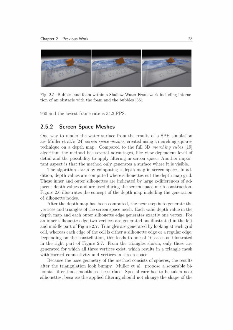
Thurey et al. [36] present a shallow water framework which is coupled toa particle-based bubble simulation. Furthermore, the bubble simulation in-teracts with a SPH simulation to handle foam floating on the fluid surface.The shallow water simulation is a reduction of the Navier-Stokes equationsto a simplified two-dimensional height field representation and represents themain volume of the liquid. Bubbles beneath the fluid surface are simulatedas particles and are coupled to the shallow water simulation. This enablesthe method to simulate breaking waves induced by bubbles reaching the fluidsurface. Foam is simulated with an SPH simulation, whereas each SPH par-ticle represents exactly one foam bubble. Foam bubbles are generated frombubbles reaching the fluid surface from beneath and the emergence is con-trolled by a user-defined probability. Simulating individual foam particles isan expensive task, in contrast our method uses the SPH particles to simulatea volume of foam and the emergence is achieved in a physical manner.

Figure 2.5 shows an example scene simulated and rendered with the shal-low water framework, whereas a 50 × 80 grid is used for the shallow watersimulation. The maximum count used for bubbles and particles is around

Chapter 2. Previous Work 23

Fig. 2.5: Bubbles and foam within a Shallow Water Framework including interac-tion of an obstacle with the foam and the bubbles [36].

960 and the lowest frame rate is 34.3 FPS.

2.5.2 Screen Space Meshes

One way to render the water surface from the results of a SPH simulationare Muller et al.’s [24] screen space meshes, created using a marching squarestechnique on a depth map. Compared to the full 3D marching cubes [19]algorithm the method has several advantages, like view-dependent level ofdetail and the possibility to apply filtering in screen space. Another impor-tant aspect is that the method only generates a surface where it is visible.

The algorithm starts by computing a depth map in screen space. In ad-dition, depth values are computed where silhouettes cut the depth map grid.These inner and outer silhouettes are indicated by large z-differences of ad-jacent depth values and are used during the screen space mesh construction.Figure 2.6 illustrates the concept of the depth map including the generationof silhouette nodes.

After the depth map has been computed, the next step is to generate thevertices and triangles of the screen space mesh. Each valid depth value in thedepth map and each outer silhouette edge generates exactly one vertex. Foran inner silhouette edge two vertices are generated, as illustrated in the leftand middle part of Figure 2.7. Triangles are generated by looking at each gridcell, whereas each edge of the cell is either a silhouette edge or a regular edge.Depending on the constellation, this leads to one of 16 cases as illustratedin the right part of Figure 2.7. From the triangles shown, only those aregenerated for which all three vertices exist, which results in a triangle meshwith correct connectivity and vertices in screen space.

Because the base geometry of the method consists of spheres, the resultsafter the triangulation look bumpy. Muller et al. propose a separable bi-nomial filter that smoothens the surface. Special care has to be taken nearsilhouettes, because the applied filtering should not change the shape of the

Chapter 2. Previous Work 24

Fig. 2.6: Left: Side view of depth map. Between adjacent nodes at most oneadditional node (white dot) is stored to indicate the silhouette (the middle whitedot represents an inner silhouette and the two other white dots outer silhouettes).Middle: Top view of the grid. Right: Side view. The cut (white point) furthestfrom the end with the smaller depth value is taken [24].

Fig. 2.7: Left: Side view of the grid. Middle: The vertices generated for thisconfiguration, whereas vertices with different depth values are generated for thesilhouette node (white point). Right: All the cases for the generation of a 2Dtriangle mesh from cut edges [24].

silhouettes, which is achieved by only considering depth values within a zmax

range (see Figure 2.6).For rendering, the resulting screen space mesh is transformed back to 3D

world space and per vertex normals are computed. Finally the triangles andnormals are sent to the standard graphics pipeline and are rendered includingreflections, refraction, and specular highlights. Figure 2.8 shows a car washscene consisting of 16k SPH particles running at 20 FPS.

Although the algorithm provides view-dependent level of detail and filter-ing in screen space, rendering foam with this approach is prohibitive, becauseof the large amount of geometry that needs to be generated.

Chapter 2. Previous Work 25

Fig. 2.8: Final rendering of the screen space mesh (including a rotated view of themesh to show its dependence on the viewing direction) [24].

2.5.3 Screen Space Fluid Rendering with Curvature Flow

van der Laan et al. [37] present an approach for rendering particle-basedfluids directly using splatting instead of performing a polygonisation andthus avoid the associated tessellation artifacts that come with grid-basedapproaches. They use screen space curvature flow filtering to conceal thesphere geometry of the particles and to prevent the fluid from looking jelly-like. All the processing, rendering and shading steps are done directly on thegraphics hardware and the method achieves real-time performance.

First of all the front-most surface of the fluid from the viewpoint of thecamera is determined. This representation is obtained by rendering all par-ticles as spheres into a depth map as illustrated in Figure 2.9. This stepis similar to the visibility splatting pass described by [4], but in the caseof screen space fluid rendering with curvature flow the depth values of thepoint-sprites are replaced by the geometry of a sphere. The hardware depthtest ensures that only the nearest pixels to the viewpoint are stored in thedepth maps. Splatting normal vectors and material properties, as it is doneby [4] in the attribute pass, is not practicable at this point, because the depthvalues of the depth map are manipulated in the following smoothing pass.

Rendering particles as point-sprites with sphere geometry results in ablobby appearance. To prevent the water from looking artificial, filteringof the surface is performed in screen-space. An obvious approach is to usea Gaussian blur, but this introduces artefacts like blurring over silhouetteedges and plateaus of equal depth when using large kernels. A more suitablemethod is the so-called curvature flow introduced by [21], which is extendedby van der Laan et al. [37] for their method. The smoothing is an iterativemethod where in each iteration the z-values in the water depth map aremoved proportional to the mean curvature,

∂z

∂t= H, (2.8)

Chapter 2. Previous Work 26

Fig. 2.9: Left: drawing particles as spheres; middle: front view in view-space;right: after perspective projection [37].

where t is a smoothing time step and H is the mean curvature. For asurface in 3D space the mean curvature is defined as follows:

2H = ∇ · n (2.9)

where n is the unit normal of the surface. The normal is calculated bytaking the cross product between the derivatives of the view space positionP in x and y direction (for details see [37]), resulting in a representation ofthe unit normal:

n(x, y) =n(x, y)

|n(x, y)| =(−Cy

∂z∂x,−Cx

∂z∂y, Cyz)

T

√D

(2.10)

where

D = C2y

(

∂z

∂x

)2

+ C2x

(

∂z

∂y

)2

+ C2xC

2yz

2 (2.11)

Finite differencing is used to calculate the spatial derivatives, and Cx andCy are the viewpoint parameters in x and y direction respectively. They arecomputed from the field of view and the size of the viewport Vx and Vy asshown in Equation 2.12 and 2.13.

Cx =2

tan(

FOV2

)

∗ Vx

(2.12)

Cy =2

tan(

FOV2

)

∗ Vy

(2.13)

The unit normal n from Equation 2.10 is substituted into Equation 2.9,which enables the derivation of H, leading to,

2H =∂nx

∂x+

∂ny

∂y=

CyEx + CxEy

D23

(2.14)

Chapter 2. Previous Work 27

in which

Ex =1

2

∂z

∂x

∂D

∂x− ∂2z

∂x2D (2.15)

Ey =1

2

∂z

∂y

∂D

∂y− ∂2z

∂y2D (2.16)

In one iteration, an Euler integration of Equation 2.8, including the meancurvature H, is used to modify the z values of the water depth map, whereasthe number of iterations is chosen depending on the smoothness that is de-sired. However, using a fixed iteration count results in different filteringstrength depending on the view distance (see Section 3.1). Discontinuities ofthe water depth map are handled by simply forcing the spatial derivativesto zero, which prevents smoothing over silhouettes in screen space. Further-more, all smoothing is computed at half instead of full resolution, which is agood tradeoff between quality and performance.

Water is a volumetric phenomenon, so the thickness of the water in frontof the opaque scene has to be taken into account. The thickness is used tocorrectly compute visual attributes like color attenuation, transparency andrefraction. To accomplish this, the particles are regarded as spheres of fluidwith a fixed size in world space and are rendered similarly as the particlesfor computing the depth values in the visibility pass described above, butinstead of writing the view-space depth value, the thickness of a particle atit’s projected position is written,

T (x, y) =n

∑

i=0

d(x− xi

σi

,y − yi

σi

) (2.17)

where d is the depth kernel function, xi and yi are the projected positioncomponents of the particle, x and y are the screen coordinates and σi is theprojected size. The summation as illustrated in Equation 2.17 is achieved byusing additive blending, and the particles are rendered with enabled depthtest and disabled depth write to ensure correct visibility with respect to thescene geometry behind the fluid.

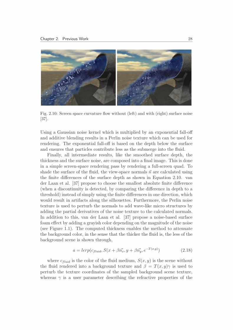
For real-time applications, the amount of particles that can be simulatedwith a SPH simulation is limited. Therefore the particles are relatively largein proportion to the complete volume of the fluid. One expects that waterhas fine micro structures on its surface which move along when the fluidflows. van der Laan et al. [37] additionally propose an approach based onPerlin noise [28] that generates noise that is advected by the fluid and is ofa higher frequency and a smaller scale than the underlying SPH simulation.They assign one octave of noise to each projected particle to establish acertain pattern of noise moving along with each particle (see Figure 2.10).

Chapter 2. Previous Work 28

Fig. 2.10: Screen space curvature flow without (left) and with (right) surface noise[37].

Using a Gaussian noise kernel which is multiplied by an exponential fall-offand additive blending results in a Perlin noise texture which can be used forrendering. The exponential fall-off is based on the depth below the surfaceand ensures that particles contribute less as the submerge into the fluid.

Finally, all intermediate results, like the smoothed surface depth, thethickness and the surface noise, are composed into a final image. This is donein a simple screen-space rendering pass by rendering a full-screen quad. Toshade the surface of the fluid, the view-space normals ~n are calculated usingthe finite differences of the surface depth as shown in Equation 2.10. vander Laan et al. [37] propose to choose the smallest absolute finite difference(when a discontinuity is detected, by comparing the difference in depth to athreshold) instead of simply using the finite differences in one direction, whichwould result in artifacts along the silhouettes. Furthermore, the Perlin noisetexture is used to perturb the normals to add wave-like micro structures byadding the partial derivatives of the noise texture to the calculated normals.In addition to this, van der Laan et al. [37] propose a noise-based surfacefoam effect by adding a grayish color depending on the magnitude of the noise(see Figure 1.1). The computed thickness enables the method to attenuatethe background color, in the sense that the thicker the fluid is, the less of thebackground scene is shown through,

a = lerp(cfluid, S(x+ β ~nx, y + β ~ny, e−T (x,y)) (2.18)

where cfluid is the color of the fluid medium, S(x, y) is the scene withoutthe fluid rendered into a background texture and β = T (x, y)γ is used toperturb the texture coordinates of the sampled background scene texture,whereas γ is a user parameter describing the refractive properties of the

Chapter 2. Previous Work 29

fluid. The optical properties of the fluid are based on the Fresnel equationand a Phong specular highlight,

Cout = a(1− F (~n · ~v)) + bF (~n · ~v) + ks(~n · ~h)α (2.19)

where a is the fluid color (containing the refracted background scenecolor) from Equation 2.18, b is the reflected scene color (sampled from anenvironment map), ks and α are constants for the specular highlight and Fis the Fresnel function controlling the composition of the reflection and therefraction component. ~n is the screen space surface normal, ~h is the half-anglevector between the camera and the light and ~v is the camera vector.

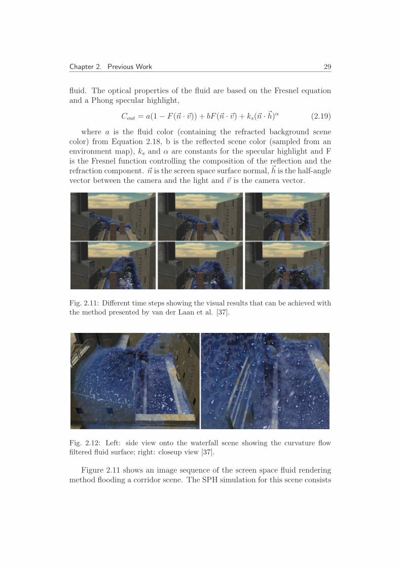
Fig. 2.11: Different time steps showing the visual results that can be achieved withthe method presented by van der Laan et al. [37].

Fig. 2.12: Left: side view onto the waterfall scene showing the curvature flowfiltered fluid surface; right: closeup view [37].

Figure 2.11 shows an image sequence of the screen space fluid renderingmethod flooding a corridor scene. The SPH simulation for this scene consists

Chapter 2. Previous Work 30

of 60k particles and an iteration count of 40 is used. The computation time isaround 19.6 ms without noise and foam (filtering is done at half resolution).Including noise and surface-based foam, the computation time is around40 ms, where the simulation time is not included in these results. Figure2.12 shows the corridor scene from different view points. The curvature flowfiltering smoothes the surface and prevents the fluid from looking “jelly-like”.However, the curvature flow filtering is dependent on the view distance (asone can see in Figure 2.12), and the proposed simple noise-based surfacefoam effect does not have a volumetric appearance (see Figure 1.1).

2.6 APIs

This section gives a brief overview of APIs realated to and used in our im-plementation. An Application Programming Interface (API) is a softwareinterface which enables a developer to access the underlying hardware andrepresents a standard for accessing and programming the hardware.

2.6.1 OpenGL

The graphics API used in the implementation is OpenGL (Open GraphicsLibrary) [26], which is a cross-platform API for writing applications thatproduce 2D and 3D computer graphics and enables a developer to programthe graphics hardware.

2.6.2 Shader Authoring Language

In the field of computer graphics, a shader is a program executed on thegraphics processing unit (GPU). Shaders supersede the fixed-function pipeline,are used to calculate rendering effects and are classified as follows:

• Vertex Shaders: Are executed exactly once for each vertex that is givento the GPU. The primary operation a vertex shader performs is totransform the world space coordinates to screen space.

• Geometry Shaders: Are used to procedurally generate new graph-ics primitives from those primitives that are processed by the vertexshader. These new graphics primitives can be points, lines or triangles.

• Fragment Shaders: Are used to calculate the output color of pixelsdelivered from the rasterizer. Common effects that are calculated withfragment shaders are Per Pixel Lighting, Bump Mapping, and more.

Chapter 2. Previous Work 31

For OpenGL, the standardized high-level shading language is the OpenGLShading Language (GLSL) [27]. It was development by the OpenGL ARBas a replacement for the low-level OpenGL Assembly Language. GLSL wasoriginally introduced as an extension to OpenGL 1.4 and since the intro-duction of OpenGL 2.0 it is part of the core. Microsoft developed the HighLevel Shading Language (HLSL) [16] for use with the DirectX API [11]. Fur-thermore, HLSL is used to develop shaders on Xbox and Xbox360. Thethird kind of shading language is the Cg Shading Language [5] developed byNVIDIA [25]. This shading language is not bound to a specific graphics APIand can be used with OpenGL and DirectX. Cg shader code is portable to awide range of platforms and the Cg compiler optimizes code automatically.Because of these benefits our implementation uses the Cg Shading Language.

Chapter 3

Method

Our method builds on the screen-space fluid rendering approach with cur-vature flow [37]. Similar to this method, we start from an SPH simulationcalculated using a hardware physics engine (PhysX [29]), which provides anon-sorted 3D point cloud as input. Apart from the particle’s position x

we will also use the density ρ and velocity v for foam thresholding and thelifetime for varying the Perlin noise on a foam particle.

The original algorithm calculates the water depth by splatting the parti-cles, then smoothes the depth buffer using curvature flow filtering, then calcu-lates water thickness by accumulating particle depths in a separate thicknessbuffer, and finally composites the results. Our algorithm extends this byadapting the curvature flow filter for the viewer distance, and by adding afoam layer that can lie between two water layers.

Our algorithm then performs the following steps once per frame after thescene has been rendered into a texture (see Figure 3.1):

1. Calculate water and foam depth (Section 3.2.2)

2. Smooth the water depth using the new adaptive curvature flow algo-rithm (Section 3.1)

3. Calculate water and foam thickness (Section 3.2.2)

4. Composite water and foam layers using intermediate results (Section 3.2.3)

In this chapter we will describe our advanced particle based water andfoam rendering approach. First of all we will introduce the adaptive curvatureflow method which extends the curvature flow filtering introduced by van derLaan et al. [37], then we will describes our real-time foam approach. Ourfoam approach is separated into the foam formation, which is carried out in aphysically based manner, the layer creation and finally the layer composition,which ensures that all the intermediate results are composed into the finalimage.

Chapter 3. Method 33

Fig.3.1:

Overview

ofthebuffersusedin

ourmethod:Twf:thicknessof

thewater

infron

tof

thefoam;Twb:thicknessofthe

water

beh

indthefoam

;Tf:foam

thickness;

Tff:thicknessof

thefron

tfoam

layer;

Chapter 3. Method 34

3.1 Adaptive Curvature Flow

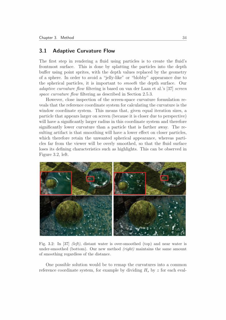
The first step in rendering a fluid using particles is to create the fluid’sfrontmost surface. This is done by splatting the particles into the depthbuffer using point sprites, with the depth values replaced by the geometryof a sphere. In order to avoid a “jelly-like” or “blobby” appearance due tothe spherical particles, it is important to smooth the depth surface. Ouradaptive curvature flow filtering is based on van der Laan et al.’s [37] screenspace curvature flow filtering as described in Section 2.5.3.

However, close inspection of the screen-space curvature formulation re-veals that the reference coordinate system for calculating the curvature is thewindow coordinate system. This means that, given equal iteration sizes, aparticle that appears larger on screen (because it is closer due to perspective)will have a significantly larger radius in this coordinate system and thereforesignificantly lower curvature than a particle that is farther away. The re-sulting artifact is that smoothing will have a lower effect on closer particles,which therefore retain the unwanted spherical appearance, whereas parti-cles far from the viewer will be overly smoothed, so that the fluid surfaceloses its defining characteristics such as highlights. This can be observed inFigure 3.2, left.

Fig. 3.2: In [37] (left), distant water is over-smoothed (top) and near water isunder-smoothed (bottom). Our new method (right) maintains the same amountof smoothing regardless of the distance.

One possible solution would be to remap the curvatures into a commonreference coordinate system, for example by dividing Hs by z for each eval-

Chapter 3. Method 35

uation of Hs. However, our experiments have shown that this makes theintegration very unstable, because the screen-space evaluation for larger par-ticles is very noisy due to depth quantization. On the other hand, depthcorrection would make the resulting curvatures large in magnitude, leadingto oscillation.

Therefore, we approach the problem from a different direction and inter-pret each integration step as a filtering step with a 3x3 kernel. Obviously,repeated filtering leads to an increased screen-space kernel radius rs of thehypothetical overall filter – in fact, the number of iterations corresponds ex-actly to rs. The main idea is now to vary the number of iterations dependingon the view space distance z in order to obtain a roughly equal overall filterkernel size rw in world space, making sure that a similar world-space neigh-borhood is taken into account when calculating the curvature flow. So rs canbe calculated from a desired world-space kernel radius rw through

rs =rw

z

FV

2(3.1)

where F is the focal length, V is the viewport width in pixels, and z

is the eye-space z-distance. So in iteration i, an Euler iteration step is onlyapplied to a pixel if rs < i. For optimization, the user can specify a maximumiteration count. Furthermore, an occlusion query is issued for each iterationto check whether any depth value was actually modified. If that is not thecase, all pixels are already converged and no further iteration is necessary.

Smoothing is only applied to the frontmost water surface. Beside thiswater depth map, a second depth map (see Figure 3.1) is computed as de-scribed in the next Section, but smoothing for this depth map is not necessarybecause it is only used as a helper depth map during the layer creation.

3.2 Real-Time Foam

In this section we describe how to incorporate foam into real-time fluid ren-dering. We define water foam as a substance that is formed by trapping airbubbles in the liquid. Foam is usually observed as spray or bubbles abovethe surface of a turbulent water stream. However, we have also observedthat a significant visual effect is caused by foam that occurs behind a watersurface, usually due to a turbulent water stream that immerges into restingwater with high impact (see Figure 3.4).

In order to capture these two main effects in a real-time setting, we sepa-rate foam particles from water particles and arrange the resulting foam andwater particles in separate layers and render them using volumetric back-to-front compositing. Although our layered representation does not account for

Chapter 3. Method 36

discontinuity in the fluid volume which occurs if there are several layers ofwater and foam, the two most common cases mentioned above are coveredby this model.

3.2.1 Foam Formation

First, we classify particles as water or foam. Following [22], we base theclassification on the Weber number [33], which is a dimensionless physicalquantity that describes the relative influence of the inertia of a fluid to itssurface tension. The Weber number is defined as the ratio of the kineticenergy to the surface energy:

We =ρv2l

σ, (3.2)

where ρ is the density, v is the relative velocity between the liquid and thesurrounding gas, l is the characteristic length, and σ is the surface tension.For larger We, the kinetic energy of the water is greater than the surfaceenergy, causing water to intermix with the surrounding air, which results infoam formation. Thus, we separate particles into water and foam particles bythresholding the Weber number. In practice, we use a linear transition areawhere the particle is counted both as water and foam particle to ensure asmooth emergence and disappearance of foam. The new foam particle startsout as a point and expands, while the corresponding water particle shrinks.

Similar to [22], we assume that the surface tension and the characteristiclength are fixed for the SPH simulation. We also assume that the characteris-tic length l is the particle diameter, which is a simplification for our real-timepurposes, and that the surrounding air is not moving, and therefore the rela-tive velocity v is the velocity of the particles. The velocity v and the densityρ are obtained from the physics simulation package.

3.2.2 Layer Creation

Now that particles have been classified as either particle or foam, we partitionthe fluid into layers, as shown in Figure 3.3.

By using two water layers, one in front and one behind the foam layer,we can simulate foam inside water, as happens at the end of a waterfall (seefor instance Figure 5.2, or Figure 3.4). We first determine the front watersurface and the front foam surface by splatting water and foam particlesinto separate depth buffers (the splatting step was described in Section 3.1).Curvature flow is only applied to the front water surface.

Chapter 3. Method 37

Fig.3.3:

Across-section

ofou

rlayered

water

model:Thevolumetricap

pearance

oftheresult

isachieved

bynotonly

accountingforthewater

thicknessTwbat

each

pixel

aspreviousap

proaches

[37],butalso

forthefoam

thicknessTfandthe

thicknessof

water

infron

tof

thefoam

Twf.Wealso

partition

foam

into

twodifferentlycoloredlayers

(Tff)to

achievemore

interestingfoam

.

Chapter 3. Method 38

Since water and foam are volumetric phenomena, the amount of water re-spectively foam between two layer surfaces needs to be determined in orderto allow correct compositing and attenuation. Similar to [37], the thick-ness of a layer is determined by additively splatting every particle belongingto the volume into a buffer. In contrast to the depth surface calculation,the splat kernel gives the thickness of the particle at each particle samplingpoint. Accumulating particle thicknesses is a reasonable approximation be-cause particles from the physics simulation can be assumed to be largelynon-overlapping.

T (x, y) =n

∑

i=0

t(x− xi

σi

,y − yi

σi

) (3.3)

where t is the particle thickness function, xi, yi are the projected positionof the particle, x and y are screen coordinates and σi is the projected size.The particle thickness function is given by

t = 2Nz l e−2r (3.4)

where Nz is the z component of the view space normal, l is the particlediameter and r is the radius, calculated form the texture coordinates, on thepoint sprite.

In comparison to [37], we not only calculate the water thickness, but thethickness of:

• the foam surface Tf , by considering only foam particles. For the foamparticles, the splat kernel is also multiplied by a 3D Perlin noise value,which is varied with the lifetime of the particle, to add sub particledetail.

• the front water surface Twf , by considering only water particles thatare in front of the foam layer (by comparing the particle depth withthe depth of the front foam surface).

• the back water surface Twb, by considering the other water particles.

• the front-most layer of the foam surface Tff , to allow partitioning foaminto two different-colored layers.

Chapter 3. Method 39

Fig.3.4:

Userdefi

ned

colors

(cfluid,cff,cfb)an

dresultingcolors

from

thecompositingstep

s(C

background,Cwb,Cf,Cwf).

Chapter 3. Method 40

3.2.3 Layer Compositing

Finally, to account for the attenuation caused by the previously calculatedlayers, the actual pixel color is calculated by volumetric compositing. Fig-ure 3.1 gives an overview of the buffers that are used for the compositing.

Compositing along a viewing ray back to front, we have (see Figure 3.3):

Cwb = lerp(cfluid, Cbackground, e−Twb) (3.5)

Cf = lerp(cfoam, Cwb, e−Tf ) (3.6)

Cwf = lerp(cfluid, Cf , e−Twf ) (3.7)

where cfoam and cfluid are the colors of the medium. Figure 3.4 shows theindividual steps and colors used in the compositing.

In addition to attenuation, we also calculate reflection with a Fresnelterm, and a highlight at the front water surface, as well as refraction, similarto [37]. For reflection and highlight, care needs to be taken because thefront water surface might be behind the foam. So if Twf = 0, we haveCwb = illuminate(Cwb), otherwise Cwf = illuminate(Cwf ), where

illuminate(x) = x(1− F (nv)) + rF (nv) + ks(nh)α, (3.8)

i.e., the standard Fresnel (F ) reflection calculation (r is a lookup intoan environment map) and a Phong term. We also carry out refraction forthe whole water surface, so Cbackground is sampled from the scene backgroundtexture perturbed along the normal vector, scaled using Twb+Twf (see Section2.5.3).

Finally, we have found that foam can be made to look more realistic byblending two different user defined colors, cff and cfb. The thickness Tff iscalculated along with the foam thicknesses Tf by accumulating just the foamparticles within a user defined constant range δfoam. So cfoam is actuallycalculated as

cfoam = lerp(cfb, cff , e−Tff ). (3.9)

By considering only foam particles which are close behind the foam sur-face, we obtain a foam pattern that has a controllable thickness, achievingthe benefit that the pattern moves along with the particles and exhibits finemicro-structures in its visual appearance.

Chapter 4

Implementation

This chapter describes the implementation of our layered particle-based fluidmodel for real-time rendering of water, including all technical implementa-tion details. All provided source/shader code listings are taken from ourimplementation, which has been developed for this thesis, and are includedin the Appendix A.

The primary logic concerning the water simulation and rendering is sep-arated into two classes:

• Fluid Class

• ScreenSpaceCurvature Class

The fluid methods and data structures provided by the physics engine areencapsulated in the Fluid class. Additionally, the physics engine provides amechanism to fragment the simulation data into packets. Each packet holdsparticles from the simulation and their location in space is represented byan axis-aligned bounding box (AABB), which can be used for view-frustumculling (see Section 4.3). The class which represents the implementation ofthe algorithm presented in this thesis is called ScreenSpaceCurvature. Thebasic program flow from the applications point of view is as follows:

• Update foam simulation (parallel to the physics sim. update; see Sec-tion 4.2)

• Update ScreenSpaceCurvature

• Render background/main scene into texture (see Section 4.4)

• Render intermediate results (see Section 4.6 and 4.8)

• Compositing (see Section 4.9)

Chapter 4. Implementation 42

• Render full-screen quad of rendering results (post-processing can beapplied in this step)

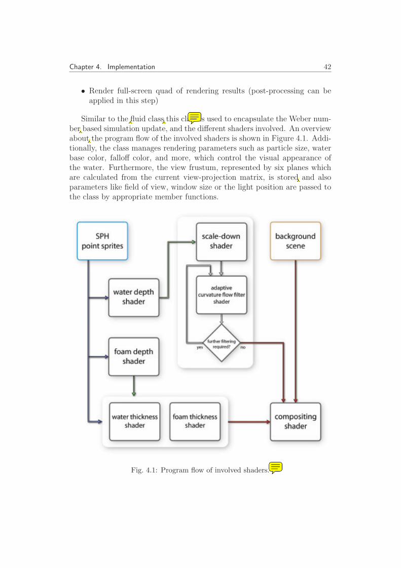
Similar to the fluid class this class is used to encapsulate the Weber num-ber based simulation update, and the different shaders involved. An overviewabout the program flow of the involved shaders is shown in Figure 4.1. Addi-tionally, the class manages rendering parameters such as particle size, waterbase color, falloff color, and more, which control the visual appearance ofthe water. Furthermore, the view frustum, represented by six planes whichare calculated from the current view-projection matrix, is stored and alsoparameters like field of view, window size or the light position are passed tothe class by appropriate member functions.

Fig. 4.1: Program flow of involved shaders.

Chapter 4. Implementation 43

4.1 Textures and Render Targets

As described in Section 3 and illustrated in Figure 3.1, all intermediate resultsare stored in textures. By default, the texture filtering modes for minificationand magnification are set to GL NEAREST to prevent unwanted filteringduring the composition pass. The same applies to the texture repeat modes,in which GL CLAMP TO EDGE is used to prevent black borders aroundthe texture.

Texture Internal Format Format

sceneTexture GL RGBA8 GL RGBAdepthTexture GL LUMINANCE32F ARB GL LUMINANCEfoamDepthTexture GL LUMINANCE32F ARB GL LUMINANCEthicknessTexture GL RGB16F ARB GL LUMINANCEfoamThicknessTexture GL RGB16F ARB GL LUMINANCEnoiseTexture GL LUMINANCE16F ARB GL LUMINANCEresultTexture GL RGBA8 GL RGBA

Tab. 4.1: Internal format and formate of textures used for intermediate results.

Table 4.1 illustrates the textures used for storing the intermediate resultsof the algorithm. In the case of the thicknessTexture and the foamThickness-Texture, GL RGB16F ARB is used as an internal format, although only twocolor channels of the three available are used. This is because there is no in-ternal format with two color channels which is usable for the algorithms pur-poses. Furthermore, the texture target isGL TEXTURE RECTANGLE ARBfor all intermediate textures and the texture dimension is equivalent to theviewport size.

For the adaptive curvature flow filtering approach additional texturesare needed to perform the downsampling (see Section 4.7). The number ofrequired downsampling textures depends on the resolution the filtering iscarried out. For instance, if the filtering is done at half resolution, one addi-tional texture is required. In the case of performing the filtering at quarterresolution two additional textures are needed to perform the downsampling.The actual filtering needs one more additional texture, which has an resolu-tion equivalent to the one at which the filtering is done. This texture andthe lowest resolution texture from the downsampling textures are used toperform multipass ping-pong rendering.

The last category of textures required by the algorithm of this thesisare helper textures, used for pattern generation and improving renderingperformance. Table 4.2 shows the textures including the parameters used

Chapter 4. Implementation 44

for creation. The foamPerlinNoise texture is an important quantity for thefoam rendering approach. As described in Section 3.2.2 it is multiplied bythe splat kernel. The texture is based on Perlin noise introduced by KenPerlin [28] and the dimension is 64x64 as illustrated in Figure 4.2.

Texture Target Internal Format Format

foamPerlinNoise TEX 3D GL RGB8 GL UNSIGNED BYTEsquareRootRamp TEX 1D GL LUMINANCE GL FLOAT

Tab. 4.2: Target, internal format and formate of used helper textures.

Fig. 4.2: FoamPerlinNoise texture.

The squareRootRamp is used during rendering to calculate the square rootof an given value in the range of [0, 1] by performing a texture lookup. Thisgives an important performance speedup, especially if the square root calcu-lation is frequently done in the fragment shader, because a texture lookupis much faster in that case. Although the accuracy of this method is not asaccurate as the accuracy of the sqrt(x) function provided by the Cg StandardLibrary [5], the accuracy is sufficiently precise for rendering tasks and doesnot introduce any visible artefacts.

As indicated in Table 4.2 the squareRootRamp is a one-dimensional tex-ture, it has a width of 128 pixels and during initialization of the applicationit is filled with the square root values between 0 and 1. Figure 4.3 gives anillustration of an squareRootRamp with a width of 16 pixels (to illustratethe discrete steps). As one can see, the resulting diagram shows a polyline,

Chapter 4. Implementation 45

which is achieved by linear interpolate pixel values if the texture lookup fallsbetween two pixels.

Fig. 4.3: Square root texture used during rendering; Top: Debug rendering of thesquareRootRamp texture; Bottom: Diagram illustrating the progress of the squareroot function.

To redirect the rendering output into rendering destination buffers theGL ARB framebuffer object (FBO) extension [15] is used. This feature en-ables the algorithm to directly render in each pass into one of the intermediatetextures.

4.2 Simulation Update

The first thing that has to be carried out at the beginning of each frame isto update the simulation. This includes to simulate one step of the physicssimulation as well as to update the Weber number-based foam simulation.The simulation data is a non-sorted 3D point cloud and each of the particleshas the following properties: position, density, velocity, lifetime, and a uniquenumber identifying the particle.

In each simulation step of the physics simulation, the properties of theparticles are updated by performing an SPH simulation. Because we build

Chapter 4. Implementation 46

on an existing physics engine which supports SPH fluid simulation, the foamsimulation is separated from the physics simulation (but could also be partof the physics simulation if the source code is available or a custom SPHimplementation is used). As described in Section 3.2.1 the foam simulationis responsible for classifying the particles as either water particles or foamparticles. The foam simulation uses its own data structure:

• FOAM : value used for fading and scaling of foam particles

• LIFETIME : lifetime that a particle has, depending on its current phase

• TIMER: timer used for accumulating the current lifetime

• PHASE : current phase of the particle

The foam phase describes in which state a particle currently is. At thebeginning a particle is counted as a water particle and its state is FP NONE.If the Weber number of the particle exceeds the user defined threshold itsstate changes to FP WATER TO FOAM. During this phase the foam valueof the particle increases from 0 to 1. After the foam value has increased to1 the particle enters the FP FOAM phase and stays in this state as long asthe Weber number is above the threshold. If the Weber number falls belowthe threshold the FP FOAM TO WATER phase is entered and the particlesfoam value is decreased until it reaches 0, whereas a user defined lifetime isused during this phase. Listing A.1 and A.2 show the main loop of the foamsimulation update.

Because of performance reasons the foam simulation is done in parallelto the physics simulation which consists of the general rigid body simulationand the fluid simulation. The drawback of this parallelism is that the foamsimulation lags one frame behind because both simulation steps work onthe same data basis and the SPH simulation buffer is locked during thesimulation step. However, close inspection of the difference between theiterative approach and the parallel one reveal that the resulting error can beneglected. The concept of the parallelism is shown in Listing A.3.

4.3 View Frustum Culling

After the simulation has been updated the data in the simulation buffersis ready for rendering. An important performance optimization is to useview frustum culling [7]. For that purpose the physics engine provides afunctionality which enables one to query for spatial data that is connectedto the fluid simulation. This spatial data is presented by packets, whereas

Chapter 4. Implementation 47

one packet is described by the NxFluidPacket structure as shown in ListingA.4. This meta data enables the algorithm to avoid to send particles downthe rendering pipeline because they are outside the camera’s frustum andtherefore are being outside of the unit cube in clipping space. Because theaxis-aligned bounding boxes (AABBs) instead of the particle positions aretested against the view frustum the number of performed frustum tests isquite small. Figure 4.4 shows a rendering of the waterfall scene including thedebug rendering of the AABBs.

Fig. 4.4: Renderings showing the AABBs provided by the physics engine. Bothfigures use the same camera viewpoint for the culling. The red AABBs are culled.

The view frustum is represented by six planes including the far and nearclip planes (defined by the standard plane equation Ax+By +Cz +D = 0,whereas ~n = (A B C) is the normal vector to the plane). As shown in ListingA.5 the algorithm iterates over all packets and tests each packet’s AABBagainst the view frustum. If the packet’s AABB is fully or partly inside theview frustum the start index and the particle count of the packet is storedfor later rendering. All packets that are fully outside the view frustum arediscarded and are ignored by all rendering passes of the algorithm.

After the simulation data has been updated and the view frustum cullinghas been carried out, the resulting data is copied to a vertex buffer object[38] (VBO). One major advantage of a VBO is that one can specify the usageof the VBO and the VBO memory manager will choose automatically thebest memory place for the buffer. This enables the algorithm to store the

Chapter 4. Implementation 48

SPH particle data including the results of the foam simulation directly inhigh-performance memory on the GPU for rendering. Attributes such asdensity, velocity, lifetime and foam are handled as texture coordinates.

4.4 Main Scene Rendering

The first rendering task which is performed by the algorithm is to render themain scene without the water into a texture as illustrated in Figure 4.5. List-ing A.6 shows the concept of the main scene rendering, whereas everythingthat is rendered between a call to BeginRenderScene and EndRenderSceneis stored in the scene texture. Also the depth values of the main scene arestored to ensure proper visibility.

Fig. 4.5: Background scene rendered at beginning of the rendering process.

By using this concept the algorithm of this thesis can be seen as a post-processing method. A post-processing pipeline [30] applies post-processingeffects to an already rendered scene and has become a standard in modernrendering engines. Because of this analogy that both work in the same wayby rendering the main scene into a texture and performing additional com-putations on this data afterwards, our algorithm can be well integrated intoa post-processing pipeline.

Chapter 4. Implementation 49

4.5 Point Sprites

The primary primitives used by the rendering passes as described later inthis chapter are point sprites. Point sprites are an useful functionality ifthousands of particles have to be rendered. Because our method can beclassified as a splatting method, point sprites are an essential choice andthus are used by our implementation. Furthermore, point sprites give asignificant performance improvement because only one vertex has to be senddown the rendering pipeline for each particle of the SPH simulation insteadof four vertices as it would be the case with ordinary billboard rendering.

The point sprite rendering functionality is encapsulated by the Render-Particles member function of the ScreenSpaceCurvature class as shown inListing A.7. An important implementation detail which has to be addressedis that GL VERTEX PROGRAM POINT SIZE ARB has to be enabled tobe able to calculate the point sprite size in the vertex shader. As describedin Section 4.3 we also use view frustum culling to reduce the particle amountthat is processed by the algorithm. vboStartIndices and vboIndexCount arearrays holding the start indices and the index count of the packets that havepassed the view frustum culling test, visiblePacketCount holds the overallpacket count.

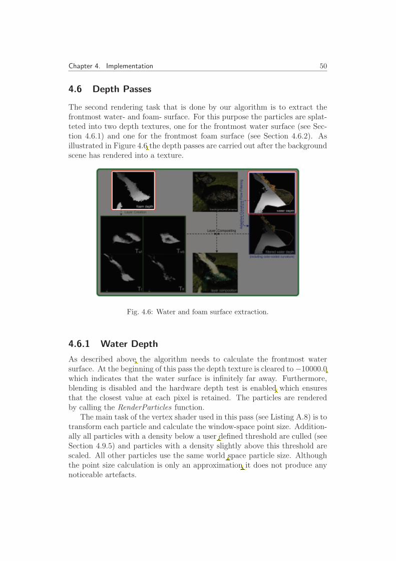
Chapter 4. Implementation 50

4.6 Depth Passes

The second rendering task that is done by our algorithm is to extract thefrontmost water- and foam- surface. For this purpose the particles are splat-teted into two depth textures, one for the frontmost water surface (see Sec-tion 4.6.1) and one for the frontmost foam surface (see Section 4.6.2). Asillustrated in Figure 4.6 the depth passes are carried out after the backgroundscene has rendered into a texture.

Fig. 4.6: Water and foam surface extraction.

4.6.1 Water Depth

As described above the algorithm needs to calculate the frontmost watersurface. At the beginning of this pass the depth texture is cleared to−10000.0which indicates that the water surface is infinitely far away. Furthermore,blending is disabled and the hardware depth test is enabled which ensuresthat the closest value at each pixel is retained. The particles are renderedby calling the RenderParticles function.

The main task of the vertex shader used in this pass (see Listing A.8) is totransform each particle and calculate the window-space point size. Addition-ally all particles with a density below a user defined threshold are culled (seeSection 4.9.5) and particles with a density slightly above this threshold arescaled. All other particles use the same world space particle size. Althoughthe point size calculation is only an approximation it does not produce anynoticeable artefacts.

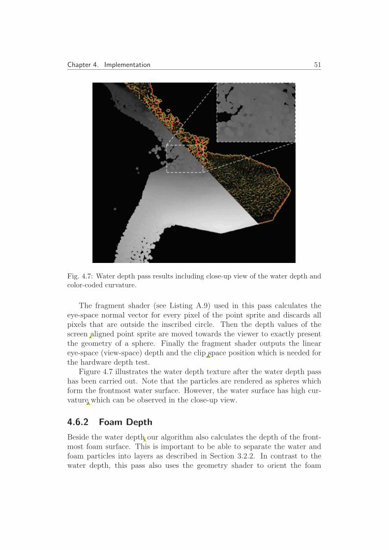
Chapter 4. Implementation 51

Fig. 4.7: Water depth pass results including close-up view of the water depth andcolor-coded curvature.

The fragment shader (see Listing A.9) used in this pass calculates theeye-space normal vector for every pixel of the point sprite and discards allpixels that are outside the inscribed circle. Then the depth values of thescreen aligned point sprite are moved towards the viewer to exactly presentthe geometry of a sphere. Finally the fragment shader outputs the lineareye-space (view-space) depth and the clip space position which is needed forthe hardware depth test.

Figure 4.7 illustrates the water depth texture after the water depth passhas been carried out. Note that the particles are rendered as spheres whichform the frontmost water surface. However, the water surface has high cur-vature which can be observed in the close-up view.

4.6.2 Foam Depth

Beside the water depth our algorithm also calculates the depth of the front-most foam surface. This is important to be able to separate the water andfoam particles into layers as described in Section 3.2.2. In contrast to thewater depth, this pass also uses the geometry shader to orient the foam

Chapter 4. Implementation 52

particles toward their velocity direction. This is done by calculating fourvertices which lie on a plane parallel to the view plane and aligning themtoward the velocity direction (see Listing A.10). Flickering artefacts becauseof low velocity are prevent by thresholding the norm of the velocity and theorientation. In this case the fallback is to render a simple screen-alignedquad. Finally the geometry shader calculates the view/eye space positions,transforms them to post-perspective space and emits four new vertices. Thealignment is useful because it results in a kind of motion blur for the finalfoam rendering which is a reasonable assumption for foam rendering.

Fig. 4.8: Foam depth pass results.

In comparison to the water depth pass results the primitives are no longersquared as can be observed in Figure 4.8.

4.7 Adaptive Curvature Flow Filtering

This section describes how to perform our adaptive curvature flow filteringwhich is based on the screen space curvature flow filtering proposed by vander Laan et al. [37]. As described in Section 3.1 the purpose of our adap-tive curvature flow filtering is to hide the particle based nature of the SPH

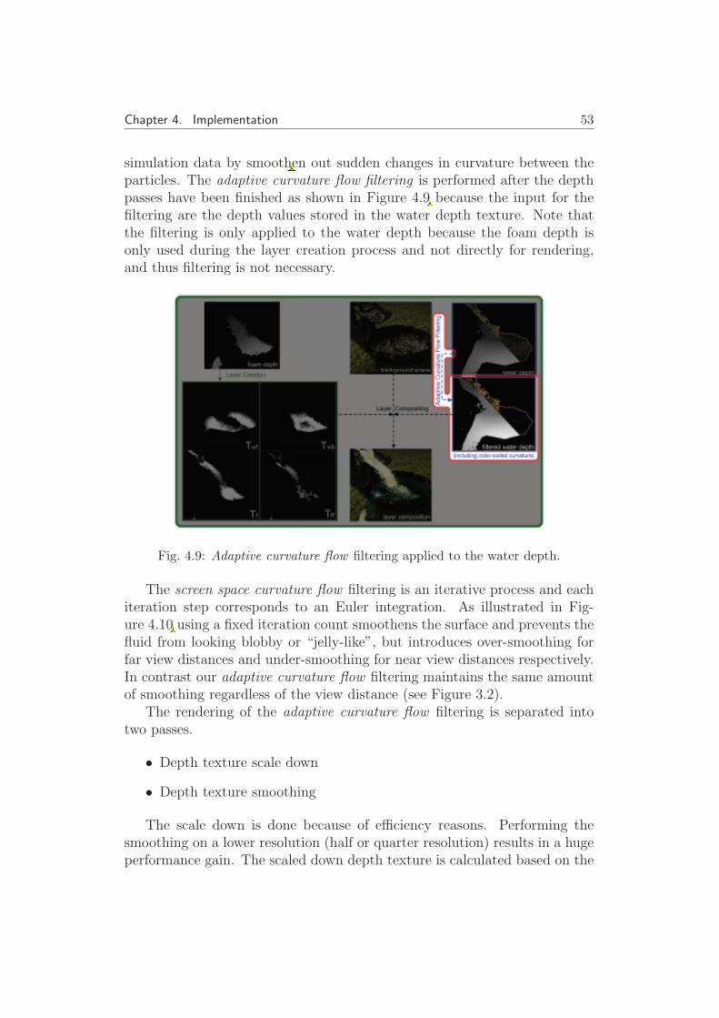
Chapter 4. Implementation 53

simulation data by smoothen out sudden changes in curvature between theparticles. The adaptive curvature flow filtering is performed after the depthpasses have been finished as shown in Figure 4.9 because the input for thefiltering are the depth values stored in the water depth texture. Note thatthe filtering is only applied to the water depth because the foam depth isonly used during the layer creation process and not directly for rendering,and thus filtering is not necessary.

Fig. 4.9: Adaptive curvature flow filtering applied to the water depth.

The screen space curvature flow filtering is an iterative process and eachiteration step corresponds to an Euler integration. As illustrated in Fig-ure 4.10 using a fixed iteration count smoothens the surface and prevents thefluid from looking blobby or “jelly-like”, but introduces over-smoothing forfar view distances and under-smoothing for near view distances respectively.In contrast our adaptive curvature flow filtering maintains the same amountof smoothing regardless of the view distance (see Figure 3.2).

The rendering of the adaptive curvature flow filtering is separated intotwo passes.

• Depth texture scale down

• Depth texture smoothing

The scale down is done because of efficiency reasons. Performing thesmoothing on a lower resolution (half or quarter resolution) results in a hugeperformance gain. The scaled down depth texture is calculated based on the

Chapter 4. Implementation 54

Fig. 4.10: Comparison of the screen space curvature flow filtering using differentfixed iteration counts as proposed by van der Laan et al. [37].

full resolution water depth texture by rendering a full-screen quad with aviewport half as large as the full screen resolution.

The next step is to calculated the actual adaptive curvature flow filter-ing. The filtering is performed until no further change happens or an upperbound of 256 iterations has been reached as illustrated in Listing A.11. Therequired iteration count is determined by using the occlusion query func-tionality provided by the OpenGL API. An occlusion query is started by acall to the glBeginQueryARB function, whereas the query is only done forevery fifth iteration in our current implementation because of performancereasons. After this the required shader parameters like the current itera-tion count (which is needed by the fragment shader to determine if furtherfiltering is required for a single pixel) are applied and a fullscreen quad isrendered. The occlusion query is stooped by a call to the glEndQueryARBfunction afterwards.

Chapter 4. Implementation 55

Because the filtering fragment shader uses the discard instruction of theCg Shading Language [5] and our upper bound calculation is based on occlu-sion queries the ping-pong rendering is not carried out in a traditional way.After the actual filtering of the water depth texture, the filtering result isonly copied to the other render target instead of directly filtering again. Inthis way it is ensured that the filtering result is correct and not overwrittenby mistake.

Fig. 4.11: Adaptive curvature flow filtered water depth including a close-up viewof the depth values, color-coded curvature, and iteration count.

The fragment shader used to perform the adaptive curvature flow filteringcalculates the necessary iteration count and smooths out sudden changes incurvature. The fragment shader is shown in Listing A.12 and Listing A.13.The first part of the fragment shader look-ups the water depth from thewater depth texture and calculates the necessary iteration count dependingon the eye-space depth as described in Section 3.1 and illustrated in Equa-tion 3.1. Because all parameters of Equation 3.1 except the eye-space depthare constant during runtime their result can be pre-calculated (stored in theshader parameter named depthFilterParam). The minus in front of the depthvalue (coo) is required because in OpenGL [26] eye-space depth values are

Chapter 4. Implementation 56

negative in front of the camera. Based on the calculated iteration count andthe current iteration count (passed as a shader parameter) a decision is madeif further filtering is necessary or the fragment has to be discarded becauseit has already converged. Additionally, eye-space depth values are discardedthat do not belong to the water surface (which is indicated by a depth valueless than −9999.0f)

The second part of the fragment shader calculates the curvature flowfiltering. First, the neighborhood depth values are looked-up and the deriva-tives are calculated by central differencing. Additionally, the directionalderivatives are calculated and tested against an user defined depth falloffto prevent filtering across the silhouettes of the water surface. These bound-ary conditions are enforced where large changes in depth occur between onefragment and the next. At these boundaries the derivatives are forced tobe zero to prevent any smoothing from taking place as proposed by van derLaan et al. [37]. Finally, the fragment shader calculates the mean curvatureas described in Section 2.5.3 and modifies the eye-space depth values of thewater depth texture. Because this process corresponds to an Euler integra-tion the mean curvature is weighted by an user defined parameter namedepsilon to prevent the filtering from oscillating.

Figure 4.11 shows the result of the adaptive curvature flow filtering. Asone can observe, the curvature of the water surface (see color-coded curvatureon the right side) is much lower in comparison to the unfiltered water depthas illustrated in Figure 4.7. Also the close-up view shows less edges and hasa smoother appearance. The subfigure shows the iteration count for thisexample viewpoint, whereas a red color indicates a higher iteration countand a yellow color a lower iteration count.

4.8 Layer Thicknesses

So far the algorithm has acquired the main scene color and extracted thewater and foam surface from the SPH data. Furthermore, the water depthhas been filtered to hide the particle-based nature of the SPH particles. Thenext step is to separate the particles into layers. As described in Section 3.2.2our algorithm separates the particles into three layers, two water layers andone foam layer in between. As shown in Figure 4.12, the input data for thispass is the previously extracted foam surface and the SPH particles. Based onthis input data the algorithm does the separation and calculates the thicknessfor each of these layers by splatting the particles and accumulating the resultinto the thickness textures. This thickness-based rendering approach givesthe viewer important information about the water deep.

Chapter 4. Implementation 57

Fig. 4.12: Layer creation based on extracted foam surface.

4.8.1 Water Layer

The water thickness pass is responsible for creating the two water layerswhich we call front water layer and back water layer (see Figure 3.3). Fromthe rendering point of view this pass is similar to the water depth pass (seeSection 4.6.1) because this pass also renders the entire set of particles. Thedifference is that this pass uses additive blending to accumulate the contri-bution of each single particle that belongs to one of the water layers into thethickness texture and also the depth write functionality is disabled. Anotherimportant difference is that the depth buffer of the main scene is used atthis point for the hardware depth test. This ensures that the thickness ofthe layers is forced to zero in regions where the water is occluded by thegeometry of the main scene.

The water thickness vertex shader is based on the water depth vertexshader (see Listing A.8). Beside the transformation and point-sprite sizecalculations the vertex shader also performs the layer separation as shownin Listing A.14. For this purpose the shader gets the foam parameter as aninput (see Section 4.2) and outputs the layer to which the particle belongsto. The actual decision to which layer the particle belongs to is calculated byusing the step function provided by the Cg Shading Language [5]. Whereasthe step functions returns 0 if the foam depth is greater than the particleseye space depth and 1 if less or equal.

The fragment shader calculates the particle thickness function as illus-trated in Figure 3.4. Instead of calculating the eye space position of the

Chapter 4. Implementation 58

Fig. 4.13: Splat kernel used for the water thickness; left: single particle; right:close-up of the back water layer thickness.

fragment on a sphere and use it as an output, the fragment shader outputstwo thickness values. As shown in Listing A.15, the thickness for each layer iscalculated based on an exponential falloff and the layer separation flag foam.In so doing, each water particle contributes to the correct water layer.

Figure 4.13 illustrates the exponential based splat kernel calculated bythe water thickness fragment shader A.15. On the left side the splat kernelfor a single particle is shown and on the right side a close-up view. Notethat by using an exponential based splat kernel the accumulated thicknessdoes not show any edges or discontinuities as one can observe in the close-upview.

Figure 4.14 illustrates the results of the water thickness pass. On the leftside the thickness of the back water layer is shown and on the right side thethickness of the front water layer respectively. Note that the water thicknessis zero for regions that are occluded by the geometry of the main scene. Thiscan be observed at the bottom of both figures where the water is occludedby the pool geometry.

4.8.2 Foam Layer

In this pass the thickness of the foam layer is calculated (see Section 3.2.2).Along with the foam thickness also the thickness in a constant range behindthe foam surface is calculated to be able to render a more realistic foam colorby blending two different user defined colors (see Section 3.2.3). Equivalentto the water thickness pass (4.8.1) additive blending, to accumulate the foamparticles, and the hardware depth test, to ensure proper occlusion by the ge-ometry of the main scene, are enabled and also the depth write functionalityis disabled. The main differences between the water thickness pass and thefoam thickness pass are that the geometry shader is used to orient the foam

Chapter 4. Implementation 59

Fig. 4.14: Water thickness pass results; left: back water layer thickness; right:front water layer thickness.

particles toward their velocity direction (as it is done in the foam depth pass4.6.2) and the splat kernel is multiplied by 3D Perlin noise.

Similar as for the water thickness vertex shader some additional calcula-tions are carried out by the foam thickness vertex shades. The vertex shaderalso looks-up the foam depth to separate the foam particles which are withina constant range behind the foam surface. This distance is passed to theshader as a parameter and defined by the user. As mentioned above thegeometry shader is used to orient the foam particles toward their velocitydirection equivalent as it is done in the foam depth pass (see Section 4.6.2).For this purpose the foam depth geometry shader as shown in Listing A.10is used because this shader does all the calculations that are required.

The foam thickness calculation done by the fragment shader, is similar tothe calculation done for the water thickness. Additionally, the exponentialfalloff is multiplied with 3D Perlin noise. A different noise pattern for eachparticle is achieved by using the lifetime of a particle for the texture look-up.The output of the foam thickness fragment shader are two thickness valuesweighted by Perlin noise. Listing A.16 shows the additional calculations doneby the foam thickness fragment shader.

Figure 4.15 illustrates the splat kernel calculated by the foam thicknessfragment shader A.16. On the left side the noise-weighted splat kernel for asingle particle is shown. Note that this pattern is only a snapshot because thepattern changes over time for each particle. The right side shows a close-upview including sub-particle detail.

Chapter 4. Implementation 60

Fig. 4.15: Splat kernel used for the foam thickness; left: single particle; right:close-up of the foam layer thickness.

Fig. 4.16: Foam thickness pass results; left: foam layer thickness; right: foamthickness in a constant range behind the foam depth.

Figure 4.16 illustrates the results of the foam thickness pass. On the leftside the thickness of the foam layer is shown and on the right side the thick-ness of the frontmost foam layer respectively. In comparison the frontmostlayer thickness is at most as thick as the depth threshold fdt, hence it is easyto normalize the frontmost layer thickness for blending by dividing it by thedepth threshold fdt (see Section 4.9). In contrast, the foam layer thicknessdoes not have an upper bound.

Chapter 4. Implementation 61

4.9 Water Rendering including Foam

In the final rendering pass all intermediate results such as the backgroundscene color, the filtered water depth and the layer thicknesses are used tocompose the actual pixel color of the water including foam (see Figure 4.17).As described in Section 3.2.3 the actual pixel color is calculated by volumet-ric compositing along a viewing ray from back to front. The compositingpass also includes real-time refraction of the background scene behind thewater, static reflections of the environment (looked-up from an static cubicenvironment map) and specular highlights based on the water surface normaland the light position.

Fig. 4.17: Compositing based on the previously calculated intermediate results.

For the compositing pass a full-screen quad is sent down the renderingpipeline similar as done for the adaptive curvature flow filtering as describedin Section 4.7. The calculations done in this pass are structured into differentparts as follows:

• Description of helper functions used for calculating eye-space positionsand interpolated normals.

• Description of the shade function (see Listing A.19 and A.20) whichcalculates the volumetric compositing as described in Section 3.2.3.

• Description of the compositing fragment shader (see Listing A.21) calledby the main programme.

Chapter 4. Implementation 62

• Description on how to incorporate shadow mapping [39] into our com-positing pass.

• Description of spray particle rendering.

4.9.1 Helper Functions

Listing A.17 shows helper functions to calculate an eye-space position. TheuvToEye function takes texture coordinates in the range [0, 1] and an eye-space depth value to calculate the eye-space position. The getEyeSpacePosfunction only takes a set of texture coordinates which are used to look-upthe eye-space depth value from the water depth texture.

The ipnormal2 function as shown in Listing A.18 calculates the partialderivatives of a normal vector based on a set of texture coordinates, a di-rectional parameter d1, and the fractional part of the texture coordinates.For this purpose, the function look-ups three eye-space depth values from thewater depth texture (eg.: left, center, middle pixel if d1 is float2(1.0f, 0.0f))and calculates as set of interpolated eye-space depth values. The output arethe interpolated partial derivatives of the water surface at the given position,which are calculated by an approximation of the central difference becauseof performance reasons.

4.9.2 Back to Front Compositing

Our method composes the different layers back to front along the viewingrays. An overview about the intermediate calculations is illustrated in Fig-ure 3.4. Note that the shader variables holding the intermediate calculationresults correspond to the labels used in this figure. Listing A.19 and A.20show the core calculations performed in the final rendering pass. The in-put parameters required to calculate the actual pixel color are the partialderivatives dxx and dyy, the eye-space position of the fragment, the tex-ture coordinates of the fragment, and a shadow term which holds informationabout shadowing. A detailed description on how to calculate the shadowingis given later in this Section.

First of all, the partial derivatives in x- and y-direction respectively areused to calculate the normal vector of the water surface. Then the eye-spaceposition and the light position (also in eye-space and passed as a shaderparameter) are used to calculate the light direction. Based on the lightdirection and the view vector the specular highlight amount is calculated.Note that the shadow amount is multiplied by the specular highlight amountto suppress specular highlights in regions which are shadowed. Furthermore,

Chapter 4. Implementation 63

the specular highlight amount is forced to zero for fragments that do nothave a valid eye-space depth value. This is required to avoid artefacts alongthe boundary of the water surface.

The next step in calculating the actual pixel color is to calculate reflec-tions of the environment. In our current implementation, static reflectionsbased on a cubic environment mapping and a Fresnel term which depends onthe viewing angle onto the water surface are used. The reflection vector issimply calculated with the reflect function (provided by the Cg Toolkit [5])based on the viewing direction and the surface normal. Note that the result-ing reflection vector has to be transformed to world-space because this is thenative space for environment maps. The Fresnel term is approximated as de-scribed in Chapter 7 of The Cg Tutorial [6] (which is also a good overview forenvironment mapping techniques and effects such as chromatic dispersion).

As described in Section 3.2.3 the compositing accounts for the attenuationcaused by the calculated layers (see Section 4.8.1 and 4.8.2). Hence, thenext step is to look-up the water thickness (representing the back water layerand the front water layer) and the foam thickness (representing the foamlayer and the frontmost foam layer). Note that not all textures have thesame dimension because the depth textures are scaled down during filtering(see Section 4.7). Thus, the texture coordinates have to be scaled to ensureproper texture look-ups. Based on the back water thickness and the frontwater thickness a refraction factor is calculated, and also the color of thebackground scene is retrieved from the scene texture which has been filledduring the main scene rendering pass as described in Section 4.4. The effectof a warped background that can be seen through the water is achieved atthis point by perturbing the texture coordinates by the surface normal vectorbefore the look-up (see Equation 2.18).

The next step is to calculate the color of the back water layer and thefront water layer which are based on a user given water color. Thus thealgorithm can produce a variety of water colors from an artistic point ofview. Beside the water layer colors, the frontmost foam surface thicknessis used to calculate the foam color as shown in Equation 3.9. Note thatthe frontmost foam surface thickness is normalize by the depth threshold asmentioned in Section 4.8.2. Additionally, the foam color is shadowed basedon an ambient color and the shadow term.

Finally, the actual pixel color is calculated by blending the intermediatecolor values together (as shown in Equation 3.7) by using the attenuationweights, which are based on the layer thickness values. At this point also thethe reflection color and the specular highlight are added.

Chapter 4. Implementation 64

4.9.3 Compositing Shader

The next part of this Section describes how the compositing fragment shaderuses the shade function as described above, to calculate the entire watersurface including foam. The primary task of the fragment shader is to sepa-rate the fluid surface into a border-region and an inner-region. This enablesthe fragment shader to avoid edge artefacts because of depth discontinuities.Next to edges colors are blended, and in the middle of the water the surfacenormals are interpolated for a smooth surface. The compositing fragmentshader is illustrated in Listing A.21.

As mentioned above the fragment shader separates the fluid surface intoa border-region and an inner-region. The separation is based on the secondderivative for three points and the derivatives are compared against a user-defined threshold.

Fig. 4.18: Border- and inner-regions separated by the compositing fragment shader.

Figure 4.18 shows an example of a separation calculated by the composit-ing fragment shader. For the red colored regions the actual pixel color iscalculated by interpolating the pixel colors of the 2×2 neighborhood aroundan fragment and interpolating them afterwards. Each color of the neighbor-hood is calculated based on the partial derivatives in x and y direction and

Chapter 4. Implementation 65

the back to front compositing described above. The process of interpolatingsamples is shown in Listing A.23 and A.24.

The yellow colored regions as illustrated in Figure 4.18 represent the innerparts of the fluid surface. The difference to border-regions is that for thoseregions the surface normals are interpolated instead of colors. The normalsare represented by their partial derivatives in the horizontal direction andthe vertical direction respectively. These partial derivatives are interpolatedbased on the fragment’s location and used to calculate the actual pixel colorfor the fluid surface.

Fig. 4.19: Compositing pass results stored in the result texture.

Finally, the compositing fragment shader outputs the actual pixel colorwhich includes specular highlights, reflection based on the Fresnel Effect,refraction of the background scene, a water surface which attenuates thebackground scene based on the thickness, and volumetric foam. Figure 4.19illustrates the results of the compositing pass. Note the volumetric appear-ance achieved by doing back-to-front compositing.

Chapter 4. Implementation 66

4.9.4 Shadowing

As mentioned at the beginning of this section, our current implementationalso handles shadows which are cast by the environment onto the water andfoam. The first part of the shadow calculation accumulates the water depthvalues of the 3×3 neighborhood and calculates an average water depth value.Because there could be the case that the fluid has regions with no water atall (in case if both water thickness values are zero and especially near bordersbecause the foam particles are orient towards their velocity direction) it hasto be checked if the average water depth value is valid. In case of an invalidaverage water depth value the routine is repeated, but instead the waterdepth values the foam depth values are used for the accumulation. Thisresults in an approximation of the fluid surface depth regardless of the layersetup which is used to calculate the shadowing (see Listing A.22).

Note that we do not go into detail onto the actual shadow calculationat this point because the fragment shader is structured in a way that anyshadow algorithm based on shadow mapping [39] is suitable and it wouldexceed the scope of this thesis. Our current implementation uses convolutionshadow maps proposed by Annen et al. [2].

4.9.5 Spray Particles

Spray particles which are indicated by a low density value normally do notform part of any surface. As mentioned by van der Laan et al. [37] it isdesirable to exclude those particles from rendering by putting a threshold onthe density obtained from the simulation. This is done in our implementationas described in Section 4.6.1 (and Listing A.8). Note that the culling of lowdensity particles is carried out in all passes which render the SPH simulationdata. The rendering of the spray particles is done immediately after thecompositing pass. Thereto the result texture from the previous pass staysbound and the spray particles are combined with the compositing results byadditive blending. The vertex shader used in this pass is very similar to thoseused for particle rendering in this Chapter expect that all particles with adensity above the user-defined threshold (instead of below) are culled. Thegeometry shader is also very similar to the one used during the foam depthpass (see Listing A.10) for example. In which the spray particles are orienttoward their velocity direction and a user-defined spray color is forwardedto the fragment shader. The fragment shader simply outputs a user-definedspray color multiplied by an exponential-based falloff.

Chapter 4. Implementation 67

Fig. 4.20: Spray particles added after the compositing pass.

Figure 4.20 illustrates the results of the spray pass. Note that the sprayparticles are blended additively with the compositing results and thereforeare much more visible on darker background colors.

Chapter 5

Results

This chapter presents results that can be achieved with our new method.First, our test setup is described, then an overview about our three scenes isgiven, and finally the chapter presents a detailed performance comparison.

We have used an Intel Q9450 CPU with a GeForce GTX 280 graphicscard. The SPH simulation was done with NVIDIA PhysX. Particle countsrange from 20k to 64k, depending on the scene. All images were takenat 1280 × 720 resolution. The curvature flow filtering step was done at halfresolution. We use off-screen buffers to store our various intermediate results:32 bit float for the water depth, 16 bit float for the foam depth, and 16 biteach for Twb, Twf , Tf and Tff . This results in a total of 112 bit per pixel.

5.1 Scenes

We have tested our approach in three different scenes. The Corridor scenehas many obstacles and therefore creates a turbulent water flow with a lot offoam and spray. The particle count used to flood this scene is around 64k andthe particles are evenly distributed in the scene. Figure 5.1 illustrates theCorridor scene. The required iteration count for the viewpoint used for thisFigure is between 27 and 52, which means that regions close to the viewpoint(as it is the case at the bottom of Figure 5.1) are filtered with 27 iterationsby our adaptive curvature flow filtering and those farther away with up to52 iterations.

The Waterfall scene is less turbulent, but due to its simplicity, artifactsare easily detected by visual inspection. Here, rendering of foam is essentialfor realistic results. In contrast to the Corridor scene, the particles are notevenly distributed in this scene, which means that most of the 64k particlesused in this scene are located in the basin at the end of the ramp construc-tion (see Figure 5.2). Another important geometric part of this scene is thepillar that holds the center ramp and splits the water flow into two streams.Due to the high compression that occurs at that position, the Weber number

Chapter 5. Results 69

Fig. 5.1: Corridor scene (27–52 iterations).

Fig. 5.2: Waterfall scene (15–20 iterations).

thresholding can be well observed. Figure 5.3 shows a comparison of the Wa-terfall scene using different values for the Weber number threshold rangingfrom 110 to 50 (see label contained in each image of Figure 5.3). Note thatthe lower the Weber number threshold, the easier foam is formed, which canbe observed especially after the pillar.

Chapter 5. Results 70

Fig. 5.3: Impact of Weber number thresholding.

Figure 5.4 shows a close-up view of the Waterfall scene. Here, one canobserve that the water surface and the foam around the pillar are shadowed.Note that in case of the water surface, the specular highlights are suppressedand the foam itself is rendered with an ambient term.

Fig. 5.4: Waterfall scene including shadowing (20–44 iterations).

Chapter 5. Results 71

The Bamboo scene consists of a bamboo construction and has dynamic el-ements that interact with the water as illustrated in Figure 5.5. The bamboois slowly filled with water, till the water weighs it down and is emptied again.Although such a scene does not produce any foam in reality, it shows thatour method can be used in scenes where the water interacts with dynamicelements. Figure 5.6 shows a close-up of the bamboo construction. Note thesmooth transition between water and foam which can be observed when theconstruction is emptied again.

Fig. 5.5: Bamboo scene (22–40 iterations).

Fig. 5.6: Bamboo scene showing water to foam transition (32–44 iterations).

Chapter 5. Results 72

Fig. 5.7: Corridor scene without/with foam (26–50 iterations).

Figure 1.1 shows the benefit of our physically guided foam generationover simple noise-based foam [37]. Figure 5.7 demonstrates that foam isan important visual element when rendering fluids. Figure 5.8 compares aphotograph of a real waterfall with our method. As one can also observe inthe photograph, the foam is visible below the surface when a turbulent waterstream immerges into resting water.

Fig. 5.8: Comparison between a photograph of a real waterfall (left) and our newmethod (right). The rectangle marks an area where foam occurs below the watersurface.

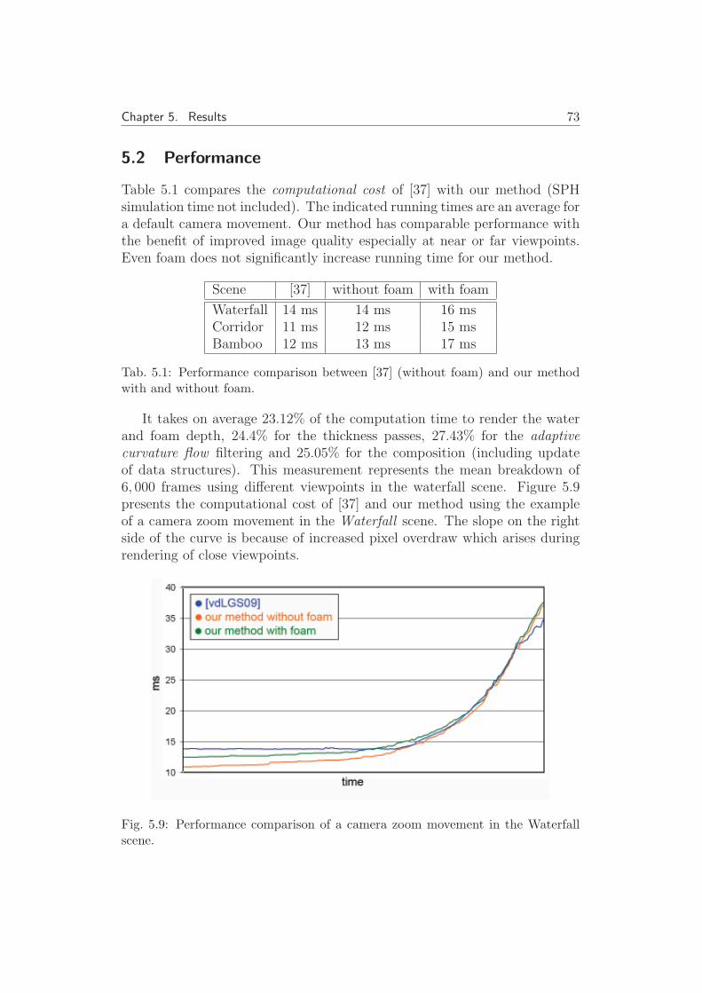
Chapter 5. Results 73

5.2 Performance

Table 5.1 compares the computational cost of [37] with our method (SPHsimulation time not included). The indicated running times are an average fora default camera movement. Our method has comparable performance withthe benefit of improved image quality especially at near or far viewpoints.Even foam does not significantly increase running time for our method.

Scene [37] without foam with foam

Waterfall 14 ms 14 ms 16 msCorridor 11 ms 12 ms 15 msBamboo 12 ms 13 ms 17 ms

Tab. 5.1: Performance comparison between [37] (without foam) and our methodwith and without foam.

It takes on average 23.12% of the computation time to render the waterand foam depth, 24.4% for the thickness passes, 27.43% for the adaptivecurvature flow filtering and 25.05% for the composition (including updateof data structures). This measurement represents the mean breakdown of6, 000 frames using different viewpoints in the waterfall scene. Figure 5.9presents the computational cost of [37] and our method using the exampleof a camera zoom movement in the Waterfall scene. The slope on the rightside of the curve is because of increased pixel overdraw which arises duringrendering of close viewpoints.

Fig. 5.9: Performance comparison of a camera zoom movement in the Waterfallscene.

Chapter 5. Results 74

Figure 5.10 presents the computational cost using a standard cameramovement through the Waterfall scene. Note that our method without foamis faster for most of the viewpoints, only if the viewpoint is close to the basinour method has increased rendering times (see right spike in Figure 5.10).

Fig. 5.10: Performance comparison of a camera movement in the Waterfall scene.

Fig. 5.11: Performance comparison of a camera movement in the Corridor scene.

Chapter 5. Results 75

Figure 5.11 presents the computational cost using a standard cameramovement through the Corridor scene. Because the viewpoints of the usedcamera movement are close to the water surface in general and the particlesare evenly distributed across the scene our method is slower.

Finally, Figure 5.12 presents the computational cost of the Bamboo scene.Note that the measurement for this scene includes the computation times ofthe physics simulation to account for the dynamic behavior and its influence.

Fig. 5.12: Performance comparison of a camera movement in the Bamboo scene,this time including physics simulation time.

5.3 Limitations

As described in Section 3.2.2, our layer model separates the fluid volumeinto three layers (two water layers and one foam layer in between). This isa reasonable approximation for most situations that appear as shown above.However, there are situations which are not covered by our layer model asshown in Figure 5.13. Here, multiple overlapping water layers are separatedby air and there is no foam layer at all. Because of this combination theentire water thickness is covered by the front water layer, which results in aninaccurate thickness calculation. To solve this artefact, it would be necessaryto calculate a filtered water surface for every water layer that occurs, whichis in fact too expensive for real-time rendering at the moment. Anotherpossible solution would be to separate the fluid volume with an approach

Chapter 5. Results 76

Fig. 5.13: Overlapping water layers separated by air. The rectangle marks an areawhere the thickness calculation is inaccurate.

based on voxelization as proposed by Eisemann et al. [13] for example. Theirapproach performs a voxelization along the viewing rays based on framebufferblending. One problem of voxelization is that not all particles might becaptured because of their relatively small size with respect to the scene sizeand the floating point precision not sufficient for this scale. However, usinga foam layer as mentioned above helps to hide those thickness artefacts asone can observe in Figure 5.7 for example.

Chapter 6

Summary and future work

In this last chapter, a summary of the thesis is given, and ideas for futurework are explored.

6.1 Conclusion

In this thesis, we presented a new physically based real-time method forrendering particle-based fluids that brings volumetric foam to the real-timedomain. Foam is an important visual element in most situations where real-time fluids are used and there exists as yet no realistic real-time method forvolumetric foam. Our algorithm is based on a previously implemented screenspace fluid rendering approach which renders the surface of particle-basedfluids and smoothes the surface to prevent the fluid from looking jelly-like.

The first contribution is an adaptive curvature flow smoothing method forSPH rendering which accounts for perspective. Instead of using a fixed itera-tion count which introduces view dependent artefacts, our adaptive methodvaries the number of iterations depending on the view distance. Thus over- orunder-smoothing as present in previous methods is avoided, and a consistentfluid surface is produced which is independent of the viewing distance.

Our second contribution is a fast physically guided foam rendering al-gorithm and a layer-based volumetric compositing algorithm. The formerclassifies particles as water or foam based on Weber number thresholding,which takes the density and velocity calculated by the physics engine intoaccount. Our layer-based model is capable of treating cases such as foamonly, water behind foam, and water in front of and behind foam. By par-titioning the fluid into a foam layer an two water layers, one in front andone behind the foam, we can simulate foam inside water, as happens at theend of a waterfall. For each layer the amount of water respectively foam isdetermined by additively splatting every particle belonging to the volume.These thickness values are used by the volumetric compositing algorithmto calculate correct compositing and attenuation along a viewing ray back

Chapter 6. Summary and future work 78

to front. Furthermore, the actual pixel color also includes reflection of theenvironment and specular highlights.

Our approach provides more realistic fluid rendering at comparable costto previous methods with the benefit of improved image quality especiallyat near or far viewpoints. Even foam does not significantly increase runningtime for our method. Our method is simple to implement and because of theanalogy that the algorithm can be seen as a post-processing method it canbe well integrated into existing rendering engines.

Fig. 6.1: Real-time rendering of caustics from reflective and refractive objects([32]).

Chapter 6. Summary and future work 79

6.2 Future Work

In future work, we plan to account for situations that require more than 3layers. This could be achieved by extending our layer approach to consider formultiple water and foam layers. The challenge with this approach is to avoidthe cost that arises if multiple water surfaces have to be filtered with ourAdaptive Curvature Flow filtering. Another solution to this problem couldbe an approach based on voxelization along the viewing rays as mentionedin Section 5.3.

In addition, we would like to investigate the achievable improvement ofusing caustics, which are an important visual element of realistic fluids. Re-cent publications like Shah et al. [32] have shown that caustics can be cal-culated efficiently in real time and with great visual quality as illustratedin Figure 6.1. Their approach avoids performing expensive geometric tests,such as ray-object intersections, and requires no pre-computation, which isimportant when dealing with fluids because the simulation is highly dynamic.

Attention has to be paid to the case if multiple water layers are overlap-ping as mentioned above. Also for caustics this has to be considered becauseeach layer reflects and refracts the incident light depending on its surfacenormal vector.

Appendix A

Shader Code

A.1 General

unsigned int fluidBufferNum = fluid->GetFluidBufferNum();

Fluid::FluidParticle* fluidBuffer = fluid->GetFluidBuffer();

const float threshold = renderDescription.foamThreshold;

const float lifetime = renderDescription.foamLifetime;

unsigned int i;

for (i=0; i<fluidBufferNum; i++)

{

const Fluid::FluidParticle& particle = fluidBuffer[i];

float weberNumber = particle.velocity.Length() *particle.velocity.Length() *particle.density;

MetaData* metaData = &fluidMetaData[particle.id];

switch (fluidMetaData[particle.id].phase)

{

case FP_NONE: // do nothing as long as weber number is low

if (weberNumber >= threshold)

{

metaData.foam = 0.0f;

metaData.lifetime = Math::RandomFloat(0.25f, 0.5f);

metaData.timer = metaData.lifetime;

metaData.phase = FP_WATER_TO_FOAM;

}

break;

...

Listing A.1: Main loop of the foam simulation update.

Appendix A. Shader Code 81

...

case FP_WATER_TO_FOAM: // fade-in foam

metaData.timer -= deltaTime;

if (metaData.timer <= 0.0f)

{

metaData.foam = 1.0f;

metaData.lifetime = metaData.timer = 0.0f;

metaData.phase = FP_FOAM;

}

else

metaData.foam = 1.0f-metaData.timer/metaData.lifetime;

break;

case FP_FOAM: // as long as weber number is high keep foam

if (weberNumber < threshold)

{

metaData.foam = 1.0f;

metaData.lifetime = Math::Clamp(lifetime*Math::

RandomFloat(0.5f, 1.5f), 0.0f, Math::MAX_FLOAT);

metaData.timer = metaData.lifetime;

metaData.phase = FP_FOAM_TO_WATER;

}

break;

case FP_FOAM_TO_WATER: // fade back to water phase

metaData.timer -= deltaTime;

if (metaData.timer <= 0.0f)

{

metaData.foam = 0.0f;

metaData.lifetime = 0.0f;

metaData.timer = 0.0f;

metaData.phase = FP_NONE;

}

else

metaData.foam = metaData.timer/metaData.lifetime;

break;

}

}

Listing A.2: Main loop of the foam simulation update. (cont.)

Appendix A. Shader Code 82

...

// run collision and dynamics for delta time since the last

// frame on the gpu (hardware)

// note that this function is non-blocking, thus the

// application can perform calculations in parallel

physicsScene->simulate(deltaTime);

// update meta data on the cpu (software)

screenSpaceCurvature->UpdateMetaData(deltaTime);

// wait for physics (fetchResults is blocking)

NxU32 error;

physicsScene->flushStream();

physicsScene->fetchResults(NX_RIGID_BODY_FINISHED, true, &

error);

...

Listing A.3: Parallelism concept.

struct NxFluidPacket

{

// AABB of all particles which are inside the same packet.

NxBounds3 aabb;

// index of first particle for a given packet.

NxU32 firstParticleIndex;

// number of particles inside the packet.

NxU32 numParticles;

// the packet’s Identifier.

NxU32 packetID;

};

Listing A.4: Data structure to represent a bounding box and its associated particledata of a fluid packet [29].

Appendix A. Shader Code 83

unsigned int numPackets = fluid->GetFluidNumPackets();

const NxFluidPacket* packets = fluid->GetFluidPackets();

unsigned int vpc = 0; // visible packet count

unsigned int i;

for (i=0; i<numPackets; i++)

{

// test intersection with view frustum

if (FrustumAABBIntersect(frustumPlanes,

Vector3(packets[i].aabb.min),

Vector3(packets[i].aabb.max)))

{

vboStartIndices[vpc] = packets[i].firstParticleIndex;

vboIndexCount[vpc] = packets[i].numParticles;

vpc++;

}

}

Listing A.5: Frustum culling functionality.

Appendix A. Shader Code 84

...

// setup render target

screenSpaceCurvature->BeginRenderScene();

{

// clear results of previous frame

glClearColor (0.0, 0.0, 0.0, 1.0);

glClear(GL_DEPTH_BUFFER_BIT | GL_COLOR_BUFFER_BIT);

...

// render scene (eg. static level geometry)

RenderManager::Instance()->Render();

...

}

// finalize rendering

screenSpaceCurvature->EndRenderScene();

...

Listing A.6: Main scene rendering concept

void ScreenSpaceCurvature::RenderParticles(void)

{

// Enable point sprite rendering

glEnable(GL_POINT_SPRITE_ARB);

// Enable point sprite size manipulation by the

// vertex shader

glEnable(GL_VERTEX_PROGRAM_POINT_SIZE_ARB);

// Render point sprites...

glMultiDrawArrays(GL_POINTS, vboStartIndices, vboIndexCount,

visiblePacketCount);

glDisable(GL_POINT_SPRITE_ARB);

glDisable(GL_VERTEX_PROGRAM_POINT_SIZE_ARB);

}

Listing A.7: Point sprite rendering function

Appendix A. Shader Code 85

A.2 Depth Passes

void FluidParticleVP(float4 position : POSITION,

float2 texCoord : TEXCOORD0,

float density : TEXCOORD1,

out float4 outPos : POSITION,

out float outPointSize : PSIZE,

out float2 outTexCoord : TEXCOORD0,

out float4 eyeSpace : TEXCOORD1)

{

outPos = mul(glstate.matrix.mvp, position);

outTexCoord = texCoord;

const float pointShrink = 0.5f;

float scaledPointRadius = particleSize * (pointShrink +

smoothstep(densityThreshold, densityThreshold*2.0f,

density)*(1.0-pointShrink));

// calculate window-space point size

float4 eyeSpacePosition = mul(glstate.matrix.modelview[0],

position);

float dist = length(eyeSpacePosition.xyz);

outPointSize = scaledPointRadius * (particleScale / dist);

eyeSpace = float4(eyeSpacePosition.xyz, scaledPointRadius);

// cull particles with density below threshold

if (density < densityThreshold)

outPos.w = -1.0;

}

Listing A.8: Water depth vertex shader

Appendix A. Shader Code 86

FragShaderOutput FluidDepthFP(float2 texCoord : TEXCOORD0,

float4 eyeSpace : TEXCOORD1)

{

FragShaderOutput OUT;

// calculate eye-space normal from texture coordinates

float3 normal;

normal.xy = texCoord.xy*float2(2.0f, -2.0f) +

float2(-1.0f, 1.0f);

float r2 = dot(normal.xy, normal.xy);

// kill pixels outside circle

if (r2 > 1.0f)

discard;

// look-up the square root for the given radius

normal.z = tex1D(sqrtMap, 1.0f-r2).x;

// position of this pixel on sphere in eye space

float4 eyeSpacePos = float4(eyeSpace.xyz +

normal*eyeSpace.w, 1.0f);

float4 clipSpacePos = mul(glstate.matrix.projection,

eyeSpacePos);

// output eye-space depth

OUT.color = float4(eyeSpacePos.z, 0.0f, 0.0f, 0.0f);

OUT.depth = (clipSpacePos.z / clipSpacePos.w)*0.5f+0.5f;

return OUT;

}

Listing A.9: Water depth fragment shader

Appendix A. Shader Code 87

POINT TRIANGLE_OUT void FluidFoamDepthGP(

AttribArray<float4> position : POSITION,

AttribArray<float4> color : COLOR0,

AttribArray<float4> prevPosition : TEXCOORD0,

AttribArray<float> pointSize : TEXCOORD1,

AttribArray<float> density : TEXCOORD2)

{

if (density[0] > densityThreshold)

{

float3 pos = position[0].xyz;

float3 prevPos = prevPosition[0].xyz;

float3 motion = pos - prevPos;

float3 direction = normalize(motion);

float len = length(motion);

float3 viewVector = normalize(-pos);

float facing = dot(viewVector, direction);

float3 x = direction*pointSize[0]*2.0f;

float3 y = normalize(cross(direction, viewVector))*pointSize[0];

const float motionThreshold = 0.5f;

if ((len < motionThreshold) || (facing > 0.95f) ||

(facing < -0.95f))

{

prevPos = pos;

x = float3(pointSize[0], 0.0, 0.0);

y = float3(0.0, -pointSize[0], 0.0);

}

float4 eyeSpace0 = float4(pos + x + y, 1.0f);

... // the same for eyeSpace1, eyeSpace2, and eyeSpace3

float4 p0 = mul(glstate.matrix.projection, eyeSpace0);

... // the same for p1, p2, and p3

emitVertex(p0, color[0], float4(0, 0, 0, 0), eyeSpace0);

emitVertex(p1, color[0], float4(0, 1, 0, 0), eyeSpace1);

emitVertex(p2, color[0], float4(1, 0, 0, 0), eyeSpace2);

emitVertex(p3, color[0], float4(1, 1, 0, 0), eyeSpace3);

}

}

Listing A.10: Foam depth geometry shader which outputs four vertices that arealigned toward the velocity direction

Appendix A. Shader Code 88

A.3 Adaptive Curvature Flow

bool breakLoop = false; bool doQuery = false;

const unsigned int queryInterval = 5;

for (int i=0; i<256 && !breakLoop; i++)

{

glBindFramebufferEXT(GL_FRAMEBUFFER_EXT, frameBuffer);

glFramebufferTexture2DEXT(...);

doQuery = (i%queryInterval == (queryInterval-1));

if (doQuery) // start occ. query

glBeginQueryARB(GL_SAMPLES_PASSED_ARB, occQuery);

... // setup shader stuff (eg.: current iteration count)

RenderQuad(scaleDownWidth, scaleDownHeight);

if (doQuery)

glEndQueryARB(GL_SAMPLES_PASSED_ARB);

srcTex = 1 - srcTex;

glFramebufferTexture2DEXT(...);

... // copy filtering result (’discard’ and occ. query)

if (doQuery)

{

unsigned int done = 0;

while (!done) // wait for occ. query result

glGetQueryObjectuivARB(occQuery,

GL_QUERY_RESULT_AVAILABLE_ARB, &done);

GLuint fragmentCount; // get occ. query result

glGetQueryObjectuivARB(occQuery , GL_QUERY_RESULT_ARB, &

fragmentCount);

breakLoop = (fragmentCount == 0);

doQuery = false;

}

srcTex = 1 - srcTex;

}

Listing A.11: Iteration loop performing the adaptive curvature flow filtering usingthe occlusion query functionality

Appendix A. Shader Code 89

FragShaderOutput FluidSmoothingFP(float2 tc : TEXCOORD0)

{

FragShaderOutput OUT;

// lookup depth value

float coo = texRECT(depthMap, IN.tc.xy).x;

// calculate necessary iteration count

float it = (depthFilterParam / -coo) + 1.0f;

// check if depth is valid and further filtering is

// necessary

if ((coo < -9999.0f) || (currentIteration > it))

{

discard;

}

else

{

...

// calculate curvature flow filtering

// (see Listing A.13)

...

}

return OUT;

}

Listing A.12: Adaptive curvature flow filtering fragment shader (showing the viewdepended iteration count calculation)

Appendix A. Shader Code 90

...

// samples

float com = texRECT(depthMap, IN.tc.xy+float2( 0.0f,-1.0f)).x;

float cmo = texRECT(depthMap, IN.tc.xy+float2(-1.0f, 0.0f)).x;

float cpo = texRECT(depthMap, IN.tc.xy+float2( 1.0f, 0.0f)).x;

float cop = texRECT(depthMap, IN.tc.xy+float2( 0.0f, 1.0f)).x;

// derivatives

float dx = (0.5f*(cpo - cmo));

float dy = (0.5f*(cop - com));

float dxx = (cmo - 2.0f*coo + cpo);

float dyy = (com - 2.0f*coo + cop);

float dxy = 0.0f;

// directional derivatives

float dx1 = coo - cmo; float dx2 = cpo - coo;

float dy1 = coo - com; float dy2 = cop - coo;

if (abs(dx1) > depthFalloff || abs(dx2) > depthFalloff)

{

dx = 0.0f; dxx = 0.0f;

}

if (abs(dy1) > depthFalloff || abs(dy2) > depthFalloff)

{

dy = 0.0f; dyy = 0.0f;

}

float depth = min(coo, thresholdMin);

float a = camera.x; float b = camera.y; float c = camera.z;

// calculate curvature

float bl = a*a*dx*dx + b*b*dy*dy + c*c*depth*depth;

float H = a*dxx*bl - a*dx*(a*a*dx*dxx + b*b*dy*dxy + c*c*depth*dx) +b*dyy*bl - b*dy*(a*a*dx*dxy + b*b*dy*dyy + c*c*depth*dy);

H /= pow(bl, 3.0f/2.0f);

// evolve under curvature

OUT.color = float4(coo + epsilon * H, 0.0f, 0.0f, 0.0f);

...

Listing A.13: adaptive curvature flow filtering fragment shader (showing thecurvature flow filtering)

Appendix A. Shader Code 91

A.4 Layer Thicknesses

...

// cull particles with density below threshold and particles

// that belong to the foam layer

if ((density < densityThreshold) || (foam > 0.0f))

outPos.w = -1.0;

// calculate texture coordinates

float3 postPerspPos = outPos.xyz / outPos.w;

float2 uv = (postPerspPos.xy*0.5f + 0.5f)*scaledDownSize;

// lookup foam depth and separate into layers

float depth = texRECT(foamDepthMap, uv).x;

outFoam = step(depth, eyeSpacePosition.z);

...

Listing A.14: Water thickness vertex shader (showing only additional calculationsto the water depth vertex shader A.8)

FragShaderOutput FluidThicknessFP(float2 texCoord : TEXCOORD0,

float foam : TEXCOORD2)

{

FragShaderOutput OUT;

// calculate eye-space normal (see Listing A.9)

...

// calculate thickness with exponential falloff

float t = normal.z*particleSize*2.0f*exp(-r2*2.0f);

// output back- and front water layer thickness

OUT.color = float4(t*(1.0f-foam), t*foam, 0.0f, 0.0f);

return OUT;

}

Listing A.15: Water thickness fragment shader (showing only different calculationsto the water depth fragment shader A.9

Appendix A. Shader Code 92

FragShaderOutput FluidThicknessFP(float4 color : COLOR0,

float2 texCoord : TEXCOORD0,

float foam : TEXCOORD2)

{

FragShaderOutput OUT;

// calculate eye-space normal (see Listing A.9)

...

// calculate thickness with exponential falloff

float t = normal.z*particleSize*2.0f*exp(-r2*2.0f);

// lookup 2D slice from perlin noise tex based on lifetime

float n = tex3D(perlinMap, float3(texCoord.xy, color.x)).x;

// output foam thickness and frontmost foam thickness

OUT.color = float4(t*n, thickness*n*color.y, 0.0f, 0.0f);

return OUT;

}

Listing A.16: Foam thickness fragment shader (showing only different calculationsto the water depth fragment shader A.9

Appendix A. Shader Code 93

A.5 Compositing

// convert [0,1] uv coords and eye-space Z

// to eye-space position

float3 uvToEye(float2 uv, float eyeZ)

{

uv = uv * invViewport;

uv = uv * float2(-2.0f, -2.0f) - float2(-1.0f, -1.0f);

return float3(uv * invFocalLength * eyeZ, eyeZ);

}

// convert [0,1] uv coords to eye-space- position

float3 getEyeSpacePos(float2 texCoord)

{

float eyeZ = texRECT(depthMap, texCoord).x;

return uvToEye(texCoord, eyeZ);

}

Listing A.17: Eye-space position calculations

float4 ipnormal2(float2 tc, float2 d1, float f1)

{

float ep1m = texRECT(depthMap, tc - d1).x;

float ep1c = texRECT(depthMap, tc).x;

float ep1p = texRECT(depthMap, tc + d1).x;

float2 dv1 = ipdepth(ep1m, ep1c, ep1p, f1);

return float4(uvToEyeD(d1, ep1c + dv1.x, ep1c), dv1.y);

}

// interpolate depth values

float2 ipdepth(float ep1m, float ep1c, float ep1p, float f1)

{

float2 d1 = float2(ep1c - ep1m, (ep1c + ep1m)*0.5f);

float2 d2 = float2(ep1p - ep1c, (ep1p + ep1c)*0.5f);

return lerp(d1, d2, f1);

}

// approx. to uvToEye(uv + uvdiff, eyeZ2) - uvToEye(uv, eyeZ)

float3 uvToEyeD(float2 uvdiff, float eyeZ2, float eyeZ)

{

return float3(invCamera*uvdiff*eyeZ, eyeZ2 - eyeZ);

}

Listing A.18: Calculate interpolated partial derivatives for normal based on texturecoordinates

Appendix A. Shader Code 94

// shade a pixel based on partial derivatives and eye position

float4 shade(float3 _ddx, float3 _ddy, float3 eyeSpacePos,

float2 texCoord, float shadowTerm)

{

float3 normal;

normal = cross(_ddx.xyz, _ddy.xyz);

normal = normalize(normal);

float3 lightDir = normalize(lightPosEyeSpace.xyz -

eyeSpacePos);

float3 v = normalize(-eyeSpacePos);

float3 h = normalize(lightDir + v);

float specular = pow(max(0.0, dot(normal, h)),

fluidShininess)*shadowTerm;

// disable specular for pixels not part of the water surface

specular *= step(-9999.0f, eyeSpacePos.z);

float fresnelTerm = fresnelBias + fresnelScale*pow(1.0 +

dot(v, normal), fresnelPower);

// cubemap reflection

float3 r = reflect(-v, normal);

r = mul((float3x3)invView, r);

float4 reflectColor = texCUBE(cubeMap, r);

// lookup water thickness from the water thickness tex

float4 thickness = texRECT(thicknessMap,

texCoord.xy*lowResFactor);

// lookup foam thickness from the foam thickness tex

float4 thicknessFoam = texRECT(foamThicknessMap,

texCoord.xy*lowResFactor);

// refraction factor

float refraction = (thickness.x+thickness.y)*thicknessRefraction;

// scene color

float4 c_scene= texRECT(sceneMap, (texCoord.xy*lowResFactor)

+ (normal.xy * refraction));

...

Listing A.19: Compositing calculation based on partial derivatives and eye position

Appendix A. Shader Code 95

...

// water back and water front fluid color

float4 c_fluid_wb = baseColor * exp(-thickness.x*falloffScale*colorFalloff);

float4 c_fluid_wf = baseColor * exp(-thickness.y*falloffScale*colorFalloff);

// foam color based on user-defined colors and blended

// based on thickness in a constant range behind the

// foam surface

float3 c_foam = lerp(foamBackColor, foamFrontColor, pow(

thicknessFoam.y*fdt, foamPowScale)).xyz;

// apply shadow term to foam color

float3 Ka = float3(0.6f, 0.6f, 0.6f);

c_foam = Ka*c_foam*(1.0f-shadowTerm) + c_foam*shadowTerm;

// attenuation factors

float att_wb = saturate(c_wb.w);

float att_foam = saturate(exp(-thicknessFoam.x*foamFalloffScale));

float att_wf = saturate(c_wf.w);

// composition

float3 c_wb = lerp(c_fluid_wb.xyz, sceneColor.xyz, att_wb);

float3 c_f = lerp(c_foam.xyz, c_wb.xyz, att_foam);

float3 c_wf = lerp(c_fluid_wf.xyz, c_f.xyz, att_wf);

// calculate factor to suppress specular highlights if

// foam is the frontmost visual element

float spw = saturate(1.0f-att_wf + att_foam)*(1.0f-att_wf);

// combine with fresnel and specular highlight

float4 surfaceColor = float4(c_wf.xyz + (reflectColor.xyz*fresnelTerm + float4(fluidSpecularColor.xyz, 1.0f).xyz*specular)*spw, 1.0f);

return c_surface;

}

Listing A.20: Compositing calculation based on partial derivatives and eye position(cont.)

Appendix A. Shader Code 96

FragShaderOutput FluidCompFP(float4 position : POSITION,

float2 texCoord : TEXCOORD0)

{

FragShaderOutput OUT;

// center tex coords and fractional part of fragment

float2 tc = floor(texCoord.xy) + 0.5f;

float2 fr = frac(texCoord.xy);

float4 fluidColor;

// texture coordinate offsets for 3x3 neighborhood

float2 texOff[9];

texOff[0] = float2( 0, 0); texOff[1] = float2(-1, 0);

texOff[2] = float2( 1, 0); texOff[3] = float2( 0,-1);

texOff[4] = float2( 0, 1); texOff[5] = float2( 1, 1);

texOff[6] = float2( 1,-1); texOff[7] = float2(-1, 1);

texOff[8] = float2(-1,-1);

// lookup depth values in 3x3 neighborhood

float depth[9];

for (int i=0; i<9; ++i)

depth[i] = texRECT(depthMap, tc + texOff[i]).x;

// calculate shadow term (see Listing A.22)

float shadowTerm = 0.0f;

...

// seperate fluid surface into border- and inner region

if(abs(depth[1] - 2.0f*depth[0] + depth[2]) > depthThresh ||

abs(depth[3] - 2.0f*depth[0] + depth[4]) > depthThresh ||

abs(depth[7] - 2.0f*depth[4] + depth[5]) > depthThresh ||

abs(depth[6] - 2.0f*depth[2] + depth[5]) > depthThresh)

{

// interpolate samples (see Listing A.23)

...

}

else

{

// interpolate normals (see Listing A.25)

...

}

OUT.color = float4(fluidColor.xyz, 1.0f);

return OUT;

}

Listing A.21: Fragment shader calculating the actual pixel color

Appendix A. Shader Code 97

float accDepthValue = 0.0f;

float accDepthNorm = 0.0f;

// average depth values 3x3 neighborhood

for (int i=0; i<9; ++i)

{

float stepValue = step(-9999.0f, depthValues[i]);

accDepthValue += depthValues[i]*stepValue;

accDepthNorm += stepValue;

}

accDepthValue /= accDepthNorm;

// if accDepthValue is invalid use foam depth instead

if (!step(-9999.0f, accDepthValue))

{

accDepthValue = 0.0f;

accDepthNorm = 0.0f;

for (int i=0; i<9; ++i)

{

float foamDepth = texRECT(foamDepthMap, tc + texOff[i]).x;

float stepValue = step(-9999.0f, foamDepth);

accDepthValue += foamDepth*stepValue;

accDepthNorm += stepValue;

}

accDepthValue /= accDepthNorm;

}

float shadowTerm = Shadow(uvToEye(texCoord, accDepthValue));

Listing A.22: Shadow term calculation

// calculate color for samples in 2x2 neighborhood

float4 s1 = sample(tc, texCoord, shadowTerm);

float4 s2 = sample(tc + texOff[2], texCoord, shadowTerm);

float4 s3 = sample(tc + texOff[4], texCoord, shadowTerm);

float4 s4 = sample(tc + texOff[5], texCoord, shadowTerm);

// interpolate samples based on fractional part of tex coords

fluidColor = lerp(lerp(s1, s2, fr.x),lerp(s3, s4, fr.x),fr.y);

Listing A.23: Sample interpolation for border regions

Appendix A. Shader Code 98

float4 sample(float2 tc, float2 texCoord, float st)

{

float3 eye = getEyeSpacePos(tc);

// calculate partial derivatives in x-direction

float3 ddx = getEyeSpacePos(tc + float2(1.0f, 0.0f)) - eye;

float3 ddx2= eye - getEyeSpacePos(tc + float2(-1.0f, 0.0f));

if(abs(ddx2.z) < abs(ddx.z)) ddx = ddx2;

// calculate partial derivatives in y-direction (see above)

...

// return sample color

return shade(ddx, ddy, eyeSpacePos, texCoord, st);

}

Listing A.24: Calculate fluid color for given texture coordinates

// calculate partial derivatives

float4 ddx = ipnormal2(tc, float2(1.0f, 0.0f), fr.x);

float4 ddx2 = ipnormal2(tc + float2(0.0f, 1.0f),

float2(1.0f, 0.0f), fr.x);

float4 ddy = ipnormal2(tc, float2(0.0f, 1.0f), fr.y);

float4 ddy2 = ipnormal2(tc + float2(1.0f, 0.0f),

float2(0.0f, 1.0f), fr.y);

// interpolate partial derivatives based on fractional part

ddx = lerp(ddx, ddx2, fr.y);

ddy = lerp(ddy, ddy2, fr.x);

// calculate eye-space position and actual color

float3 eyePos = uvToEye(texCoord, (ddx.w + ddy.w)*0.5f);

fluidColor = shade(ddx.xyz, ddy.xyz, eyePos, texCoord,

shadowTerm);

Listing A.25: Normal interpolation for inner regions

List of Figures

1.1 A scene rendered with simple noise-based foam [37] (left) andwith our new method (right); . . . . . . . . . . . . . . . . . . 10

2.1 Ocean scene simulated with two-way coupling between theSPH and the particle level set method [20]. . . . . . . . . . . . 18

2.2 Diver performing a jump into a pool [22]. . . . . . . . . . . . . 202.3 A piece of lumber falling into water [35]. . . . . . . . . . . . . 212.4 Ale and Stout pouring into a beer mug [8]. . . . . . . . . . . . 212.5 Bubbles and foam within a Shallow Water Framework includ-

ing interaction of an obstacle with the foam and the bubbles[36]. . . . . . . . . . . . . . . . . . . . . . . . . . . . . . . . . 23

2.6 Left: Side view of depth map. Between adjacent nodes atmost one additional node (white dot) is stored to indicate thesilhouette (the middle white dot represents an inner silhouetteand the two other white dots outer silhouettes). Middle: Topview of the grid. Right: Side view. The cut (white point)furthest from the end with the smaller depth value is taken [24]. 24

2.7 Left: Side view of the grid. Middle: The vertices generated forthis configuration, whereas vertices with different depth valuesare generated for the silhouette node (white point). Right: Allthe cases for the generation of a 2D triangle mesh from cutedges [24]. . . . . . . . . . . . . . . . . . . . . . . . . . . . . . 24

2.8 Final rendering of the screen space mesh (including a rotatedview of the mesh to show its dependence on the viewing di-rection) [24]. . . . . . . . . . . . . . . . . . . . . . . . . . . . . 25

2.9 Left: drawing particles as spheres; middle: front view in view-space; right: after perspective projection [37]. . . . . . . . . . 26

2.10 Screen space curvature flow without (left) and with (right)surface noise [37]. . . . . . . . . . . . . . . . . . . . . . . . . . 28

2.11 Different time steps showing the visual results that can beachieved with the method presented by van der Laan et al. [37]. 29

2.12 Left: side view onto the waterfall scene showing the curvatureflow filtered fluid surface; right: closeup view [37]. . . . . . . . 29

List of Figures 100

3.1 Overview of the buffers used in our method: Twf : thicknessof the water in front of the foam; Twb: thickness of the waterbehind the foam; Tf : foam thickness; Tff : thickness of thefront foam layer; . . . . . . . . . . . . . . . . . . . . . . . . . 33

3.2 In [37] (left), distant water is over-smoothed (top) and nearwater is under-smoothed (bottom). Our new method (right)maintains the same amount of smoothing regardless of thedistance. . . . . . . . . . . . . . . . . . . . . . . . . . . . . . . 34

3.3 A cross-section of our layered water model: The volumetricappearance of the result is achieved by not only accounting forthe water thickness Twb at each pixel as previous approaches[37], but also for the foam thickness Tf and the thickness ofwater in front of the foam Twf . We also partition foam intotwo differently colored layers (Tff ) to achieve more interestingfoam. . . . . . . . . . . . . . . . . . . . . . . . . . . . . . . . . 37

3.4 User defined colors (cfluid, cff , cfb) and resulting colors fromthe compositing steps (Cbackground, Cwb, Cf , Cwf ). . . . . . . . 39

4.1 Program flow of involved shaders. . . . . . . . . . . . . . . . . 424.2 FoamPerlinNoise texture. . . . . . . . . . . . . . . . . . . . . . 444.3 Square root texture used during rendering; Top: Debug ren-

dering of the squareRootRamp texture; Bottom: Diagram il-lustrating the progress of the square root function. . . . . . . . 45

4.4 Renderings showing the AABBs provided by the physics en-gine. Both figures use the same camera viewpoint for theculling. The red AABBs are culled. . . . . . . . . . . . . . . . 47

4.5 Background scene rendered at beginning of the rendering pro-cess. . . . . . . . . . . . . . . . . . . . . . . . . . . . . . . . . 48

4.6 Water and foam surface extraction. . . . . . . . . . . . . . . . 504.7 Water depth pass results including close-up view of the water

depth and color-coded curvature. . . . . . . . . . . . . . . . . 514.8 Foam depth pass results. . . . . . . . . . . . . . . . . . . . . . 524.9 Adaptive curvature flow filtering applied to the water depth. . 534.10 Comparison of the screen space curvature flow filtering using

different fixed iteration counts as proposed by van der Laanet al. [37]. . . . . . . . . . . . . . . . . . . . . . . . . . . . . . 54

4.11 Adaptive curvature flow filtered water depth including a close-up view of the depth values, color-coded curvature, and itera-tion count. . . . . . . . . . . . . . . . . . . . . . . . . . . . . . 55

4.12 Layer creation based on extracted foam surface. . . . . . . . . 57

List of Figures 101

4.13 Splat kernel used for the water thickness; left: single particle;right: close-up of the back water layer thickness. . . . . . . . . 58

4.14 Water thickness pass results; left: back water layer thickness;right: front water layer thickness. . . . . . . . . . . . . . . . . 59

4.15 Splat kernel used for the foam thickness; left: single particle;right: close-up of the foam layer thickness. . . . . . . . . . . . 60

4.16 Foam thickness pass results; left: foam layer thickness; right:foam thickness in a constant range behind the foam depth. . . 60

4.17 Compositing based on the previously calculated intermediateresults. . . . . . . . . . . . . . . . . . . . . . . . . . . . . . . . 61

4.18 Border- and inner-regions separated by the compositing frag-ment shader. . . . . . . . . . . . . . . . . . . . . . . . . . . . . 64

4.19 Compositing pass results stored in the result texture. . . . . . 654.20 Spray particles added after the compositing pass. . . . . . . . 67

5.1 Corridor scene (27–52 iterations). . . . . . . . . . . . . . . . . 695.2 Waterfall scene (15–20 iterations). . . . . . . . . . . . . . . . . 695.3 Impact of Weber number thresholding. . . . . . . . . . . . . . 705.4 Waterfall scene including shadowing (20–44 iterations). . . . . 705.5 Bamboo scene (22–40 iterations). . . . . . . . . . . . . . . . . 715.6 Bamboo scene showing water to foam transition (32–44 itera-

tions). . . . . . . . . . . . . . . . . . . . . . . . . . . . . . . . 715.7 Corridor scene without/with foam (26–50 iterations). . . . . . 725.8 Comparison between a photograph of a real waterfall (left)

and our new method (right). The rectangle marks an areawhere foam occurs below the water surface. . . . . . . . . . . 72

5.9 Performance comparison of a camera zoom movement in theWaterfall scene. . . . . . . . . . . . . . . . . . . . . . . . . . . 73

5.10 Performance comparison of a camera movement in the Water-fall scene. . . . . . . . . . . . . . . . . . . . . . . . . . . . . . 74

5.11 Performance comparison of a camera movement in the Corri-dor scene. . . . . . . . . . . . . . . . . . . . . . . . . . . . . . 74

5.12 Performance comparison of a camera movement in the Bam-boo scene, this time including physics simulation time. . . . . 75

5.13 Overlapping water layers separated by air. The rectanglemarks an area where the thickness calculation is inaccurate. . 76

6.1 Real-time rendering of caustics from reflective and refractiveobjects ([32]). . . . . . . . . . . . . . . . . . . . . . . . . . . . 78

List of Tables

4.1 Internal format and formate of textures used for intermediateresults. . . . . . . . . . . . . . . . . . . . . . . . . . . . . . . . 43

4.2 Target, internal format and formate of used helper textures. . 44

5.1 Performance comparison between [37] (without foam) and ourmethod with and without foam. . . . . . . . . . . . . . . . . . 73

List of Listings

A.1 Main loop of the foam simulation update. . . . . . . . . . . . 80A.2 Main loop of the foam simulation update. (cont.) . . . . . . . 81A.3 Parallelism concept. . . . . . . . . . . . . . . . . . . . . . . . . 82A.4 Data structure to represent a bounding box and its associated

particle data of a fluid packet [29]. . . . . . . . . . . . . . . . . 82A.5 Frustum culling functionality. . . . . . . . . . . . . . . . . . . 83A.6 Main scene rendering concept . . . . . . . . . . . . . . . . . . 84A.7 Point sprite rendering function . . . . . . . . . . . . . . . . . . 84A.8 Water depth vertex shader . . . . . . . . . . . . . . . . . . . . 85A.9 Water depth fragment shader . . . . . . . . . . . . . . . . . . 86A.10 Foam depth geometry shader which outputs four vertices that

are aligned toward the velocity direction . . . . . . . . . . . . 87A.11 Iteration loop performing the adaptive curvature flow filtering

using the occlusion query functionality . . . . . . . . . . . . . 88A.12 Adaptive curvature flow filtering fragment shader (showing the

view depended iteration count calculation) . . . . . . . . . . . 89A.13 adaptive curvature flow filtering fragment shader (showing the

curvature flow filtering) . . . . . . . . . . . . . . . . . . . . . . 90A.14 Water thickness vertex shader (showing only additional calcu-

lations to the water depth vertex shader A.8) . . . . . . . . . 91A.15 Water thickness fragment shader (showing only different cal-

culations to the water depth fragment shader A.9 . . . . . . . 91A.16 Foam thickness fragment shader (showing only different cal-

culations to the water depth fragment shader A.9 . . . . . . . 92A.17 Eye-space position calculations . . . . . . . . . . . . . . . . . 93A.18 Calculate interpolated partial derivatives for normal based on

texture coordinates . . . . . . . . . . . . . . . . . . . . . . . . 93A.19 Compositing calculation based on partial derivatives and eye

position . . . . . . . . . . . . . . . . . . . . . . . . . . . . . . 94A.20 Compositing calculation based on partial derivatives and eye

position (cont.) . . . . . . . . . . . . . . . . . . . . . . . . . . 95A.21 Fragment shader calculating the actual pixel color . . . . . . . 96

List of Listings 104

A.22 Shadow term calculation . . . . . . . . . . . . . . . . . . . . . 97A.23 Sample interpolation for border regions . . . . . . . . . . . . . 97A.24 Calculate fluid color for given texture coordinates . . . . . . . 98A.25 Normal interpolation for inner regions . . . . . . . . . . . . . . 98

Bibliography

[1] Tomas Akenine-Moller and Eric Haines. Real-Time Rendering 2nd Edi-tion. A. K. Peters, Ltd., Natick, MA, USA, 2002.

[2] Thomas Annen, Tom Mertens, Philippe Bekaert, Hans-Peter Seidel, andJan Kautz. Convolution shadow maps. In Rendering Techniques 2007:Eurographics Symposium on Rendering, pages 51–60, Grenoble, France,2007. Eurographics.

[3] Florian Bagar, Daniel Scherzer, and Michael Wimmer. A layeredparticle-based fluid model for real-time rendering of water. In ComputerGraphics Forum (Proceedings EGSR 2010), volume 29, June 2010.

[4] Mario Botsch, Alexander Hornung, Matthias Zwicker, and Leif Kobbelt.High-quality surface splatting on today’s gpus. In Symposium on Point-Based Graphics 2005, pages 17–24, June 2005.

[5] Cg Toolkit. http://developer.nvidia.com/object/cg_toolkit.html.

[6] The Cg Tutorial: Environment Mapping Techniques. http://http.

developer.nvidia.com/CgTutorial/cg_tutorial_chapter07.html.

[7] James H. Clark. Hierarchical geometric models for visible surface algo-rithms. Commun. ACM, 19(10):547–554, 1976.

[8] Paul W. Cleary, Soon Hyoung Pyo, Mahesh Prakash, and Bon Ki Koo.Bubbling and frothing liquids. ACM Trans. Graph., 26(3):97, 2007.

[9] Mathieu Desbrun and Marie-Paule Gascuel. Smoothed particles: a newparadigm for animating highly deformable bodies. In Proceedings ofthe Eurographics workshop on Computer animation and simulation ’96,pages 61–76, New York, NY, USA, 1996. Springer-Verlag New York, Inc.

[10] P. Dirac. Principles of quantum mechanics. Oxford at the ClarendonPress, 1958.

[11] Microsoft DirectX. http://msdn.microsoft.com/directX.

Bibliography 106

[12] Yoshinori Dobashi, Kazufumi Kaneda, Hideo Yamashita, TsuyoshiOkita, and Tomoyuki Nishita. A simple, efficient method for realisticanimation of clouds. In SIGGRAPH ’00: Proceedings of the 27th annualconference on Computer graphics and interactive techniques, pages 19–28, New York, NY, USA, 2000. ACM Press/Addison-Wesley PublishingCo.

[13] Elmar Eisemann and Xavier Decoret. Single-pass gpu solid voxelizationfor real-time applications. In GI ’08: Proceedings of graphics interface2008, pages 73–80, Toronto, Ont., Canada, Canada, 2008. CanadianInformation Processing Society.

[14] Kenny Erleben, Jon Sporring, Knud Henriksen, and Henrik Dohlmann.Physics Based Animation. Charles River Media, 2005.

[15] Framebuffer Object. http://www.opengl.org/registry/specs/ARB/

framebuffer_object.txt.

[16] High Level Shading Language. http://msdn.microsoft.com/en-us/

library/bb509561%28v=VS.85%29.aspx.

[17] Henrik Wann Jensen. Realistic Image Synthesis Using Photon Mapping.AK Peters, Ltd, 2001.

[18] Daniel D. Joseph. Questions in fluid mechanics: Understanding foamsand foaming. Journal of Fluids Engineering, 119:497–498, 1997.

[19] William E. Lorensen and Harvey E. Cline. Marching cubes: A high reso-lution 3d surface construction algorithm. SIGGRAPH Comput. Graph.,21(4):163–169, 1987.

[20] Frank Losasso, Jerry Talton, Nipun Kwatra, and Ronald Fedkiw. Two-way coupled sph and particle level set fluid simulation. IEEE Transac-tions on Visualization and Computer Graphics, 14(4):797–804, 2008.

[21] Ravi Malladi and James A. Sethian. Level set methods for curvatureflow, image enhancement, and shape recovery in medical images. pages329–ff., 1997.

[22] Viorel Mihalef, Dimitris N. Metaxas, and Mark Sussman. Simulationof two-phase flow with sub-scale droplet and bubble effects. Comput.Graph. Forum, 28(2):229–238, 2009.

[23] J. J. Monaghan. Smoothed particle hydrodynamics. araa, 30:543–574,1992.

Bibliography 107

[24] Matthias Muller, Simon Schirm, and Stephan Duthaler. Screen spacemeshes. In SCA ’07: Proceedings of the 2007 ACM SIGGRAPH/Euro-graphics symposium on Computer animation, pages 9–15, Aire-la-Ville,Switzerland, Switzerland, 2007. Eurographics Association.

[25] NVIDIA Corporation. http://www.nvidia.com/page/home.html.

[26] OpenGL. http://www.opengl.org/.

[27] The OpenGL Shading Language. http://www.opengl.org/registry/

doc/GLSLangSpec.4.00.7.pdf.

[28] Ken Perlin. An image synthesizer. SIGGRAPH Comput. Graph.,19(3):287–296, 1985.

[29] NVIDIA PhysX. http://developer.nvidia.com/object/physx.html.

[30] Creating A Post-Processing Framework. http://www.gamasutra.com/

view/feature/1812/creating_a_postprocessing_.php?page=1.

[31] Simon Premoze, Tolga Tasdizen, James Bigler, Aaron Lefohn, andRoss T. Whitaker. Particle-based simulation of fluids, 2003.

[32] Musawir A. Shah, Jaakko Konttinen, and Sumanta Pattanaik. Causticsmapping: An image-space technique for real-time caustics. IEEE Trans-actions on Visualization and Computer Graphics, 13:272–280, 2007.

[33] William A Sirignano. Fluid dynamics and transport of droplets andsprays, 1999. Incluye referencias bibliograficas (p. 287-307) e ındice (p.309-311).

[34] Jos Stam. Stable fluids. In SIGGRAPH ’99: Proceedings of the 26th an-nual conference on Computer graphics and interactive techniques, pages121–128, New York, NY, USA, 1999. ACM Press/Addison-Wesley Pub-lishing Co.

[35] Tsunemi Takahashi, Hiroko Fujii, Atsushi Kunimatsu, Kazuhiro Hi-wada, Takahiro Saito, Ken Tanaka, and Heihachi Ueki. Realistic anima-tion of fluid with splash and foam. Comput. Graph. Forum, 22(3):391–400, 2003.

[36] N. Thurey, F. Sadlo, S. Schirm, M. Muller-Fischer, and M. Gross. Real-time simulations of bubbles and foam within a shallow water framework.In SCA ’07: Proceedings of the 2007 ACM SIGGRAPH/Eurograph-ics symposium on Computer animation, pages 191–198, Aire-la-Ville,Switzerland, Switzerland, 2007. Eurographics Association.

Bibliography 108

[37] Wladimir J. van der Laan, Simon Green, and Miguel Sainz. Screen spacefluid rendering with curvature flow. In I3D ’09: Proceedings of the 2009symposium on Interactive 3D graphics and games, pages 91–98, NewYork, NY, USA, 2009. ACM.

[38] Vertex Buffer Object. http://www.opengl.org/registry/specs/ARB/

vertex_buffer_object.txt.

[39] Lance Williams. Casting curved shadows on curved surfaces. SIG-GRAPH Comput. Graph., 12(3):270–274, 1978.

[40] T. Yabe. Universal solver cip for solid, liquid and gas. ComputationalFluid Dynamics Review 1997 Ed. By M. M. Hafez and K. Oshima, 1997.

Acknowledgements

”All we have to decide is what to do with the time that isgiven to us.”

– Gandalf the Grey, ”The Lord of the Rings: The Fellowship of the Ring”

First, I want to thank Daniel Scherzer for making this diploma thesis possi-ble and helping me to publish our new approach at the ”21st EurographicsSymposium on Rendering” which took place from June 28th 2010 – June30th 2010 in Saarbrucken.

Secondly, thanks to Michael Wimmer for giving me great support during thepaper submission and helping to improve the quality of our paper.

Thanks to all my co-workers at Spriong for giving me the possibility to learnso much from them during the last four years. Extra acknowledgment toRaimund Schumacher for his great feedback which helped to enhance thequality of my work and to Johannes Graf which helped me with his artisticskills.

Last but not least, I would like to thank all my friends and my family for alltheir great support over the past years.