VALUATION OF LIFE INSURANCE POLICIES MODEL … · Valuation of Life Insurance Policies Model Regulation

A Law of Large Numbers approach tovaluation in life insurance
Tom Fischer∗
Heriot-Watt University, Edinburgh
First version: March 17, 2003This version: February 17, 2006
Abstract
The classical Principle of Equivalence ensures that a life insurancecompany can accomplish that the mean balance per policy convergesto zero almost surely for an increasing number of independent policy-holders. By certain assumptions, this idea is adapted to the generalcase with stochastic financial markets. The implied minimum fair priceof general life insurance policies is then uniquely determined by theproduct of the assumed unique equivalent martingale measure of thefinancial market with the physical measure for the biometric risks. Theapproach is compared with existing related results. Numeric examplesare given.
JEL: G10, G13, G22Subj. Class.: IM01, IM10, IM12, IM30, IB10
MSC: 91B24, 91B28, 91B30Key words: Hedging, Law of Large Numbers, life insurance,
Principle of Equivalence, valuation
1 Introduction
Roughly speaking, the Principle of Equivalence of traditional life insurancemathematics states that premiums should be calculated such that incomesand losses are “balanced in the mean”. Under the assumption that financialmarkets are deterministic, this idea leads to a valuation method usually called
∗The author gratefully acknowledges funding by the German Federal Ministry of Ed-ucation and Research (BMBF, 03LEM6DA), and support by J. Lehn and A. May. Fur-thermore, suggestions from an unknown referee substantially improved the paper. Corre-spondence to: Tom Fischer, Department of Actuarial Mathematics and Statistics, Heriot-Watt University, Edinburgh EH14 4AS, United Kingdom; Tel: +44 131 451 4371; Email:[email protected]
1

1 INTRODUCTION 2
“Expectation Principle”. The use of the two principles ensures that a life officecan accomplish that (i.e. can buy hedges such that) the mean balance per policyconverges to zero almost surely for an increasing number of policyholders. Thisis often confered to as the ability to “diversify” mortality (or biometric) risks.The main mathematical ingredients for this diversification are the stochasticindependence of individual lives and the Strong Law of Large Numbers (SLLN).To obtain the mentioned convergence, it is neither necessary to have identicalpolicies, nor to have i.i.d. lifetimes.
In modern life insurance mathematics, where financial markets are assumedto be stochastic and where more general products (e.g. unit-linked ones) aretaken into consideration, the widely accepted valuation principle is an expec-tation principle, too. However, the respective probability measure is differentsince the minimum fair price or market value of an insurance claim is deter-mined by the no-arbitrage pricing method known from financial mathematics.The respective equivalent martingale measure (EMM) is the product of thegiven EMM of the financial market with the physical measure for the biomet-ric risks. Throughout the paper, we will call this kind of valuation the productmeasure principle. Although the result is not as straightforward as in the tra-ditional case, a convergence property similar to the one mentioned above canbe shown. So, diversification of biometric risks is still possible in the presenceof stochastic financial markets, where payments related to e.g. unit-linked lifepolicies of different policyholders may not be independent.
The aim of this paper is the derivation of an equivalent martingale mea-sure for the pricing of life insurance policies starting from the assumptionthat, under the induced valuation principle, diversification of biometric risksshould be possible by means of a convergence property as above, i.e. a lifeinsurance company should be able to accomplish that the mean balance percontract converges to zero almost surely for an increasing number of indepen-dent policyholders. We will see that, under certain assumptions, the EMMthen is uniquely determined and given by the product measure mentioned ear-lier, i.e. by the product of the given EMM of the financial market with thephysical measure for the biometric risks. In different versions, diversificationapproaches have appeared in the literature on valuation. Considered as some-how straightforward, they are usually stated without proofs and for identicalpolicies and i.i.d. lives, only. However, the derivation of a unique equivalentmartingale measure and respective convergence properties for varying typesof policies and lives at the same time, as carried out in this paper, needs aformally different setup and different mathematical tools than the derivationof a unique pricing rule for infinitely many identical policies for i.i.d. lives, asdone in some papers. In this sense, the present paper has a technical focus.Particular emphasis is put on mathematically rigorous and explicit model as-sumptions necessary for the derivation of the mentioned results. For instance,we state integrability conditions for cash flows of not necessarily identical poli-cies that are sufficient for the application of the SLLN even if independencegets lost by common financial risks.

1 INTRODUCTION 3
Research on the valuation of unit-linked life insurance products alreadystarted in the late 1960s. One of the first results that was in its core identicalto the product measure principle was Brennan and Schwartz (1976). In thispaper, the authors ”eliminate mortality risk” by assuming an “average pur-chaser of a policy”, which clearly is a diversification argument. More recentpapers mainly dedicated to valuation following this approach are Aase andPersson (1994) for the Black-Scholes model and Persson (1998) for a stochas-tic interest rate model. Aase and Persson (1994), but also other authors, apriori suppose independence of financial and biometric events. In their paper,an arbitrage-free and complete financial market ensures the uniqueness of thefinancial EMM. The product measure principle is here motivated by a diversi-fication argument, but also by “risk-neutrality” of the insurer with respect tobiometric risks (cf. Aase and Persson (1994), Persson (1998)). A more detailedhistory of valuation in (life) insurance can be found in Møller (2002), see alsothe references therein.
There exist other derivations of the product measure principle which donot rely on diversification arguments. In Møller (2001), for example, theproduct measure coincides with the so-called minimal martingale measure(cf. Schweizer, 1995b). The works Møller (2002, 2003a, 2003b) also considervaluation, but focus on hedging (mainly quadratic criteria), respectively ad-vanced premium principles. Becherer (2003) uses exponential utility functionsto derive prices of contracts. In an example for a certain type of contract fori.i.d. lives, he shows that the product measure principle evolves in the limitfor infinitely many policyholders. In general, no-arbitrage pricing of insurancecash flows using martingales and equivalent martingale measures, was intro-duced by Delbaen and Haezendonck (1989) and Sondermann (1991). Later,Steffensen (2000) described possible sets of price operators for life insurancecontracts by respective sets of eqivalent martingale measures. A more detaileddiscussion of some valuation approaches, among them Steffensen (2000) andBecherer (2003), will take place in Section 8.
The present paper works with a discrete finite time framework. Like otherpapers in this field, it is general in the sense that it does not propose partic-ular models for the dynamics of financial securities or biometric events. Theconcept of a life insurance policy is introduced in a very general way and thepresented methods are not restricted to particular types of contracts. Thediversification approach is carried out by assuming certain properties (mostof them also assumed in the articles cited above) of the underlying stochasticmodel, like e.g. independence of individuals, independence of biometric and fi-nancial events, no-arbitrage pricing, etc. To be able to model a wide variety ofpossible types of policies and lives, we assume an infinite product space for thebiometric risks that also provides for each possible life (of which we may haveinfinitely many) infinitely many i.i.d. ones (= large cohorts of similar lives).In fact, the setting is that we consider biometric probability spaces (= lives)and random variables on their products with the financial probability space(= policies). As already said, the resulting product measure valuation prin-

2 SOME PRINCIPLES 4
ciple is in accordance with existing results. Because of no-arbitrage pricing,not only prices at time 0, but complete price processes are determined. Underthe mentioned assumptions, it is then shown how a life insurance companycan accomplish the earlier described convergence of mean balances of hedgestogether with contractual payments. The initial costs of the respective purelyfinancial and self-financing hedging strategies can be financed by the minimumfair premiums.
The hedging method considered in this paper is different from the risk-minimizing and mean-variance hedging strategies in Møller (1998, 2001, 2002).In fact, the method is a discrete generalization of the matching approach inAase and Persson (1994). This method is less sophisticated than e.g. riskminimizing strategies (which are unfortunately not self-financing), but is prac-ticable in the sense that not every single life has to be observed over the wholeterm. The paper provides examples for pricing and hedging of different typesof policies. A more detailed example shows for a term assurance and an en-dowment the historical development of the ratio of the minimum fair annualpremium per benefit. Assuming that premiums are calculated by a conserva-tively chosen constant technical rate of interest, the example also derives thedevelopment of the market values, i.e. minimum fair prices, of these contracts.
The section content is as follows. In Section 2, some principles consideredto be reasonable for a basic theory of life insurance are briefly discussed in anenumerated list. Section 3 introduces the market model and the first mathe-matical assumptions concerning the stochastic model of financial and biomet-ric risks (product space). Section 4 defines general life insurance policies andstates a generalized Principle of Equivalence (cf. Persson, 1998). In Section5, the case of classical life insurance mathematics and the motivation of theExpectation Principle by risk diversification, i.e. the Law of Large Numbers,is briefly reviewed. Section 6 contains the Law of Large Numbers approachto valuation in the general case and the deduction of the minimum fair price(product measure principle). In particular, it is explained how the Strong Lawof Large Numbers can be properly applied in the introduced product spaceframework. Section 7 is about hedging, i.e. about the convergence of meanbalances. In this section, examples are given, too. In Section 8, we discussrelated results in the present literature on derivation of valuation principles.In Section 9, it is shown how parts of the results can be adapted to the caseof incomplete markets. Even for markets with arbitrage opportunities someresults still hold. Section 10 is dedicated to the numerical pricing examplementioned above. The last section is the conclusion. The appendix containsfigures.
2 Some principles
The following eight principles informally describe the biometric and financialframework of this article. The formulation by mathematical assumptions
2 SOME PRINCIPLES 5
follows later. It is clear that the principles of our model are not perfect orcomplete in any sense, and a considerable amount of research is carried outin areas where this might be particularly true, e.g. thinking of the idealizedassumption of independent individual biometry (principle 3) which is stronglychallenged by the evidence of so-called longevity risk (e.g. Richards and Jones,2004). However, the proposed model should be seen as a rudimentary lifeinsurance framework inheriting some basic ideas and idealized assumptionsfrom the classical theory, but already working with stochastic financialmarkets. In this sense, it is a modern framework. Each principle is given witha short explanation motivating it.
1. Independence of biometric and financial events. Biometric (ortechnical) events, for instance death or injury of persons, are assumed to bestochastically independent of the events of the financial markets (cf. Aase andPersson, 1994). In contrast to reinsurance companies, where the movements onthe financial markets can be highly correlated to technical events (e.g. earth-quakes), such effects are rather unlikely in the case of life insurance.
2. Complete arbitrage-free financial markets. Except for Section 9,where incomplete markets are examined, complete and arbitrage-free financialmarkets are considered throughout the paper. Even though this might bean unrealistic assumption from the viewpoint of finance, it is realistic fromthe perspective of life insurance. The reason is that a life insurance companyusually does not invent purely financial products as this is the working field ofbanks. Therefore, it can be assumed that all considered financial products areeither traded on the market, can be bought from banks or can be replicatedby self-financing strategies. Nonetheless, it is self-evident that a claim whichalso depends on a biometric event (e.g. the death of a person) can not behedged by financial securities, i.e. the joint market of financial and biometricrisks is not complete. In the literature, completeness of financial markets isoften assumed by the use of the Black-Scholes model (cf. Aase and Persson(1994), Møller (1998)). However, parts of our results are also valid in the caseof incomplete financial markets - which allows for more models. In this case,financial portfolios will be restricted to replicable ones, and also the consideredlife insurance policies are restricted in a similar way.
3. Biometric states of individuals are independent. This is thestandard assumption of classical life insurance. Neglecting the possibility ofepidemic diseases or wars, the principle could be held for appropriate in a mod-ern framework, too. However, recently research is carried out on modelling andmanaging risk caused by major demographic developments (see also the intro-ductory remark above). In this case, more realistic models with dependenciesfairly enough should replace the biometric independence assumption. Nonethe-less, we stay with this assumption as our main argument uses diversifyabilityof biometric risks and claims to be traditional with respect to this.
4. Large classes of similar individuals. Applying the Law of LargeNumbers in classical life insurance mathematics, an implicit assumption is

2 SOME PRINCIPLES 6
a large number of persons under contract in a particular company. Evenstronger, it can usually be assumed that classes of “similar” persons, e.g. of thesame age, gender and health status, are large. An insurance company shouldbe able to cope with such a large cohort of similar persons even if all membersof the cohort have the same kind of policy (see also Principle 7 below).
5. Similar individuals can not be distinguished. For fairness reasons,any two individuals with similar biometric development to be expected shouldpay the same price for the same kind of contract. Furthermore, any activity(e.g. hedging) taken by an insurance company for two individuals holding thesame kind of policy is assumed to be identical as long as their possible futurebiometric development is independently identical from the stochastic point ofview.
6. No-arbitrage pricing. As we know from the theory of financial mar-kets, an important property of a reasonable pricing system is the absence ofarbitrage, i.e. the absence of riskless wins. In our case, it should not be possibleto beat the market by selling and buying life insurance products in e.g. an ex-isting or hypothetical reinsurance market (cf. Delbaen and Haezendonck (1989)and Sondermann (1991)). Hence, any product and cash flow will be priced orgiven a value under the no-arbitrage principle.
7. Minimum fair prices allow hedging such that mean balancesconverge to zero almost surely. The principle of independence of thebiometric probability spaces is closely related to the Expectation Principleof classical life insurance mathematics. In the classical case, where financialmarkets are assumed to be deterministic, this principle states that the valueor single net premium of a cash flow is the expectation of the sum of itsdiscounted payoffs (expected present value). The connection between the twoprinciples is the Law of Large Numbers. Values or prices are determined suchthat for an increasing number of contracts issued to independent individualsthe insurer can accomplish that the mean final balance per policy converges tozero almost surely (the variance of this mean balance converges to null, too).In analogy to the classical case, we generally demand that the minimum fairprice of any policy (from the viewpoint of the insurer) should at least coverthe price of a purely financial hedging strategy that lets the mean balance perpolicy converge to zero a.s. for an increasing number of policyholders.
8. Principle of Equivalence. Under a reasonable valuation principle(cf. Principle 7), the Principle of Equivalence demands that the future pay-ments to the insurer (premiums) should be determined such that their (mar-ket) value equals the (market) value of the future payments to the insured(benefits). The idea is that the liabilities (benefits, claims) can somehow behedged working with the premiums. In the coming sections, this concept willbe considered in detail.
Remark 1. In the theory of deterministic financial markets, today’s (time 0)price of a future cash flow is called its present value. The value of a future cashflow also subject to mortality risk, evaluated with the classical ExpectationPrinciple, is called its expected present value. The value of the same cash flow

3 THE MODEL 7
evaluated with principles of modern life insurance mathematics (stochasticfinancial markets) is called market value in the literature since evaluation isusually done using market prices of related securities which do not containbiometric risks. However, the notion market value is somehow misleading asthe life insurance contracts themselves are usually not traded and hence thereusually exist no prices for them that are directly determined by the market. Inaccordance with Principle 7, we will call the market value also the minimumfair price.
Remark 2. Concerning premium calculation, the classical Expectation Prin-ciple (cf. Principle 7) is usually seen as a minimum premium principle sinceany insurance company must be able to cope with higher expenses than theexpected (cf. Embrechts, 2000). So-called safety loads on the minimum fairpremiums can be obtained by more elaborate premium principles. We referto the literature for more information on the topic (e.g. Delbaen and Haezen-donck (1989); Gerber (1997); Goovaerts, De Vylder and Haezendonck (1984);Møller (2002-2003b); Schweizer (2001)). Another possibility to obtain safetyloads is to use the Expectation Principle with a prudent first order base (also:technical base or premium basis) for biometric and financial developments,e.g. conservatively chosen mortality and interest rates, that represent a worst-case scenario for the future development of the second order base (experiencebase), that stands for the real, i.e. observed, development (e.g. Norberg, 2001).
3 The model
Let (F,FT , F) be a probability space equipped with the filtration (Ft)t∈T, whereT = {0, 1, 2, . . . , T} denotes the discrete finite time axis. Assume that F0 istrivial, i.e. F0 = {∅, F}. Let the price dynamics of d securities of a frictionlessfinancial market be given by an adapted Rd-valued process S = (St)t∈T. Thed assets with price processes (S0
t )t∈T, . . . , (Sd−1t )t∈T are traded at times t ∈
T \ {0}. The first asset with price process (S0t )t∈T is called the money account
and has the properties S00 = 1 and S0
t > 0 for t ∈ T. The tuple MF =(F, (Ft)t∈T, F, T, S) is called a securities market model. A portfolio in MF
is given by a d-dimensional vector θ = (θ0, . . . , θd−1) of real-valued randomvariables θi (i = 0, . . . , d−1) on (F,FT , F). A t-portfolio is a portfolio θt whichis Ft-measurable. As usual, Ft is interpreted as the information available attime t. Since an economic agent takes decisions with respect to the informationavailable, a trading strategy is a vector θT = (θt)t∈T of t-portfolios θt. Thediscounted total gain (or loss) of such a strategy is given by
∑T−1t=0 〈θt, St+1−St〉,
where S := (St/S0t )t∈T denotes the price process discounted by the money
account and 〈. , .〉 denotes the inner product on Rd. One can now define
G =
{T−1∑t=0
〈θt, St+1 − St〉 : each θt is a t-portfolio
}. (1)

3 THE MODEL 8
G is a subspace of the space of all real-valued random variables L0(F,FT , F)where two elements are identified if they are equal F-a.s. The process S satisfiesthe so-called no-arbitrage condition (NA) if G ∩ L0
+ = {0}, where L0+ are the
non-negative elements of L0(F,FT , F) (cf. Delbaen, 1999). The FundamentalTheorem of Asset Pricing (Dalang, Morton and Willinger, 1990) states thatthe price process S satisfies (NA) if and only if there is a probability measureQ equivalent to F such that under Q the process S is a martingale. Q is calledequivalent martingale measure (EMM), then. Moreover, Q can be found withbounded Radon-Nikodym derivative dQ/dF.
DEFINITION 1. A valuation principle πF on a set Θ of portfolios in MF
is a linear mapping which maps each θ ∈ Θ to an adapted R-valued stochasticprocess (= price process) πF (θ) = (πF
t (θ))t∈T such that
πFt (θ) = 〈θ, St〉 =
d−1∑i=0
θiSit (2)
for any t ∈ T for which θ is Ft-measurable.
For the moment, the set Θ is not specified any further.
Remark 3. Observe that θ is not indexed with some t as we just assumeit to be FT -measurable in general. For instance, in a case where θ is FT -measurable, but not FT−1-measurable, the valuation principle πF would assigna value πF
T−1(θ) to θ although it could not be observed at time T − 1. This iscomparable to the case where we assign a value (at time T − 1) to an optionor insurance contract maturing at time T although we not yet know the finaloutcome of the contract.
Consider an arbitrage-free market with price process S as given aboveand a portfolio θ with price process πF (θ). From the Fundamental The-orem it is known that the enlarged market with price dynamics S ′ =((S0
t , . . . , Sd−1t , πF
t (θ)))t∈T is arbitrage-free if and only if there exists an EMMQ for S ′, i.e. Q ∼ F and S ′ a Q-martingale. Hence, one has
πFt (θ) = S0
t · EQ[〈θ, ST 〉/S0T |Ft]. (3)
It is well-known that the no-arbitrage condition does not imply a uniqueprice process for θ when the portfolio can not be replicated by a self-financingstrategy θT, i.e. a strategy such that 〈θt−1, St〉 = 〈θt, St〉 for each t > 0 andθT = θ. However, in a complete market MF , i.e. a market which featuresa self-financing replicating strategy for any portfolio θ (cf. Lemma 1), theno-arbitrage condition implies unique prices (where prices are identified whenequal a.s.) and therefore a unique EMM Q. Actually, an arbitrage-freesecurities market model as introduced above is complete if and only if theset of equivalent martingale measures is a singleton (cf. Harrison and Kreps(1979); Taqqu and Willinger (1987); Dalang, Morton and Willinger (1990)).

3 THE MODEL 9
We will now introduce assumptions which concern the properties of marketmodels (not of valuation principles) that include biometric events (cf. Princi-ples 1 to 4 of Section 2).
Assume to be given a filtered probability space (B, (Bt)t∈T, B) which de-scribes the development of the biological states of all considered human beings.No particular model for the development of the biometric information is as-sumed.
ASSUMPTION 1. A common filtered probability space
(M, (Mt)t∈T, P) = (F, (Ft)t∈T, F)⊗ (B, (Bt)t∈T, B) (4)
of financial and biometric events is given, i.e. M = F ×B, Mt = Ft ⊗ Bt andP = F⊗ B. Furthermore, F0 = {∅, F} and B0 = {∅, B}.
As M0 = {∅, F ×B}, the model implies that the world is known for sure attime 0. The symbols M,Mt and P are introduced to shorten notation. M andMt are chosen since these objects describe events of the underlying marketmodel, whereas P denotes the physical probability measure. Later, M is usedto denote a martingale measure.
ASSUMPTION 2. A complete securities market model
MF = (F, (Ft)t∈T, F, T, F S) (5)
with a unique equivalent martingale measure Q is given. The common marketmodel for financial and biometric risks is denoted by
MF×B = (M, (Mt)t∈T, P, T, S), (6)
where S(f, b) = F S(f) for all (f, b) ∈ M .
In the following, MF×B is understood as a securities market model. Thenotions portfolio, no-arbitrage etc. are used as introduced at the beginning ofthis section. We will need the following lemma.
LEMMA 1.
(i) Any Ft-measurable portfolio can be replicated by a self-financing strategyin MF until t.
(ii) Any Ft-measurable payoff can be replicated by a self-financing strategy inMF until t.
Proof. (i) As MF is complete, any FT -measurable payoff X at T can be repli-cated until T . This is the usual definition of the completeness of a securitiesmarket model. Hence, there exists for any Ft-measurable portfolio θt a replicat-ing self-financing (s.f.) strategy (ϕt)t∈T in MF , i.e. ϕT = θt, since X = 〈θt, ST 〉could be chosen. For no-arbitrage reasons, one must have πF
s (θt) = 〈ϕs, Ss〉for s ∈ T and therefore 〈θt, Ss〉 = 〈ϕs, Ss〉 for any s ≥ t. So, there also existsa s.f. strategy such that ϕt = θt, i.e. the portfolio θt is replicated until t.(ii) Due to (i), the portfolio θt = X/S0
t · e0 can for any Ft-measurable payoffX be replicated until t. Observe that 〈θt, St〉 = X.

4 LIFE INSURANCE POLICIES 10
Remark 4. S is the canonical embedding of F S into (M, (Mt)t∈T, P). Wewill usually use the same symbol for a random variable X in (F,Ft, F) anda random variable Y in (M,Mt, P) (t ∈ T) when Y is the embedding of Xinto (M,Mt, P), i.e. Y (f, b) = X(f) for all (f, b) ∈ M . Now, any portfolio F θof the complete financial market MF can be replicated by some self-financingtrading strategy F θT = (F θt)t∈T. Under (NA), the unique price process πF (F θ)of the portfolio is given by
πFt (F θ) = F S0
t · EQ[〈F θ, F ST 〉/F S0T |Ft]. (7)
Since S is the embedding of F S into (M, (Mt)t∈T, P), the embedded portfolio
F θ in MF×B is replicated by the embedded trading strategy F θT = (F θt)t∈Tin MF×B. Hence, to avoid arbitrage opportunities, any reasonable valuationprinciple π must feature a price process π(F θ) in MF×B that fulfills πt(F θ) =πF
t (F θ) P-a.s. for any t ∈ T. Since EQ[X|Ft] = EQ⊗B[X|Ft⊗B0] P-a.s. for anyrandom variable X in (F,FT , F), one must have P-a.s.
πt(F θ) = S0t · EQ⊗B[〈F θ, ST 〉/S0
T |Ft ⊗ B0] (8)
= S0t · EQ⊗B[〈F θ, ST 〉/S0
T |Ft ⊗ Bt].
Observe that (St/S0t )t∈T is a Q⊗ B-martingale.
ASSUMPTION 3. There are infinitely many human individuals and we have
(B, (Bt)t∈T, B) =∞⊗i=1
(Bi, (Bit)t∈T, Bi), (9)
where BH = {(Bi, (Bit)t∈T, Bi) : i ∈ N+} is the set of filtered probability spaces
describing the development of the i-th individual (N+ := N \ {0}). Each Bi0 is
trivial.
It follows that B0 is also trivial, i.e. B0 = {∅, B}.
ASSUMPTION 4. For any space (Bi, (Bit)t∈T, Bi) in BH there are infinitely
many isomorphic (=identical, except for the indices) ones in BH .
In the sense of Remark 2, the four assumptions above define a model forthe second order base.
4 Life insurance policies
Under the setup given in the last section, the biometric development has bydefinition no influence on the price process S of the financial market - and viceversa. We therefore have situations where a portfolio θ that contains biometricrisk - that is a portfolio which is not of the form θ = F θ P-a.s. with F θ anMF -portfolio - can not be replicated by purely financial products. Hence, in

4 LIFE INSURANCE POLICIES 11
general, relative pricing of life insurance products with respect to MF is notpossible. Usually, life insurance policies are not traded and the possibility ofthe valuation of such contracts by the market is not given. The market MF×B
of financial and biometric risks is incomplete. Nonetheless, products have tobe priced as e.g. the insured usually have the right to dissolve any contractat any time of its duration. We are therefore in the need of a reasonablevaluation principle π for the considered portfolios Θ of the market MF×B andin particular for general life insurance products.
DEFINITION 2. A general life insurance policy is a vector (γt, δt)t∈Tof pairs (γt, δt) of t-portfolios in Θ (to shorten notation we drop the innerbrackets of ((γt, δt))t∈T). For any t ∈ T, the portfolio γt is interpreted asa payment of the insurer to the insurant (benefit) and δt as a payment ofthe insurant to the insurer (premium), respectively taking place at t. Thenotation (iγt,
iδt)t∈T means that the contract depends on the i-th individual’slife, i.e. for all (f, x), (f, y) ∈ M
(iγt(f, x), iδt(f, x))t∈T = (iγt(f, y), iδt(f, y))t∈T (10)
whenever pi(x) = pi(y), pi being the canonical projection of B onto Bi.
For any policy (γt, δt)t∈T issued by a life office to an individual, this streamof payments is from the viewpoint of the insurer equivalent to holding theportfolios (δt − γt)t∈T.
Although there has not yet been considered any particular valuation prin-ciple, it is assumed that a suitable principle π is a minimum fair price in theheuristic sense given in Section 2, Principle 7. The properties of a minimumfair price will be defined and further explained in Section 6.
ASSUMPTION 5. Suppose a suitable valuation principle π on Θ. For anylife insurance policy (γt, δt)t∈T the Principle of Equivalence demands that
π0
(T∑
t=0
γt
)= π0
(T∑
t=0
δt
). (11)
As already mentioned in Section 2 (Principle 8), the idea of Eq. (11) isthat the liabilities (γt)t∈T can somehow be hedged working with the premiums(δt)t∈T since their present values or market values are identical. For the classicalcase, this idea is explained in the next section.
Remark 5. We use portfolio notation (and not cash flow notation) since e.g. aunit-linked life insurance policy depends usually on shares of a fund whichare combinations of traded assets. Trading and hedging strategies becomemore transparent with this notation. Furthermore, later stated integrabilityconditions can be formulated for units of a portfolio, rather than for a combinedgeneral cash flow. We think, this makes the application of these conditionseasier (compare Examples 3, 4, and Remark 10).

5 VALUATION: THE CLASSICAL CASE 12
Since portfolio notation is not commonly used in life insurance mathemat-ics, we give a brief example of an application of Eq. (11) for a unit-linkedassurance.
Example 1 (Portfolio notation for a unit-linked assurance). We useAssumptions 1 and 2. For T = 2 and d = 2, assume a complete and arbitrage-free securities market model MF , e.g. a Cox-Ross-Rubinstein model, with twoassets, the first one being deterministic (bond, S0), the second one stochastic(stock, S1). We consider a life aged x. This life is modelled by the filtered space(B, (Bt)t∈{0,1,2}, B), and we assume that he or she is alive at time 0. Supposenow that β is B1-measurable with β(b) ∈ {0, 1} for any b ∈ B. Assume thatβ = 1 if and only if the individual is alive at 1. Define now γ0 = (0, 0),γ1 = (0, 1000(1 − β)) and γ2 = (0, 1500β). Furthermore, δ0 = (P, 0), whereP ∈ R, and δ1 = δ2 = (0, 0). These portfolios define a simple unit-linkedassurance for the considered life. The policy features a single premium of P attime 0, the benefit of 1000 shares at time 1 if the life has died until then, or, ifthis was not the case, the benefit of 1500 shares at time 2. For the calculationof P by (11), we will use the product measure principle, which will be discussedin detail later. Hence, we assume that π is given by
πt(θ) = S0t · EQ⊗B[〈θ, S2〉/S0
2 |Ft ⊗ Bt], t ∈ {0, 1, 2}. (12)
Therefore,
π0
(2∑
t=0
γt
)= π0
(2∑
t=0
δt
)(13)
π0 (1000(0, 1− β + 1.5β)) = π0 ((P, 0))
1000EQ⊗B[(1 + 0.5β)S12/S
02 ] = P.
From this we obtain
P = 1000EB[1 + 0.5β]EQ[S12/S
02 ] (14)
= 1000(1 + 0.5EB[β])S10
= 1000S10 + px500S1
0 ,
where px = EB[β] is international actuarial notation for the probability thatan individual aged x survives the following year. Hence, the single premium is1000 times the share price at time zero, plus 500 times the share price at time0 multiplied with the one-year survival probability of the life (x). This reflectsthe policy, that pays 1000 shares for sure, either at time 1 or at time 2, andan additional 500 shares at time 2 if the policyholder survived the first year.
5 Valuation: the classical case
In classical life insurance mathematics, the financial market is assumed to bedeterministic. We realize this assumption by |FT | = 2, i.e. FT = {∅, F}, and

5 VALUATION: THE CLASSICAL CASE 13
identify (M, (Mt)t∈T, P) with (B, (Bt)t∈T, B). As the market is assumed to befree of arbitrage, all assets must have the same dynamics up to scaling factors.Hence, we can assume S = (S0
t )t∈T, i.e. d = 1 and the only asset is the moneyaccount as a deterministic function of time. In the classical framework, it iscommon sense that the fair value (or price) at time s of a B-integrable payoffCt at t is the conditional expectation of the discounted payoff with respect toBs, i.e. for a t-portfolio Ct/S
0t , having the value Ct at t, we have
πs(Ct/S0t ) := S0
s · EB[Ct/S0t |Bs], s ∈ T. (15)
Under the Expectation Principle (15), the classical Principle of Equivalence isgiven by (11). As the discounted price processes are B-martingales, the classi-cal financial market together with a finite number of classical price processesof life policies is free of arbitrage opportunities.
Let us have a closer look at the logic of valuation principle (15). Assumethat Θ is given by the B-integrable portfolios. Suppose Assumption 1 to 3 andconsider the claims {(−iγt)t∈T : i ∈ N+} of a policy from the companies pointof view, where iγt depends on the i-th individual’s life, only (cf. Definition 2).Furthermore, suppose that for all t ∈ T there is a ct ∈ R+ such that
||iγt||2 ≤ ct (16)
for all i ∈ N+, where ||.||2 denotes the L2-norm of the Hilbert spaceL2(M,MT , P) of all square-integrable real functions on (M,MT , P). Now,buy for all i ∈ N+ and all t ∈ T the portfolios EB[iγt], where EB[iγt] is inter-preted as a financial product (a t-portfolio) which matures at time t, i.e. thepayoff EB[iγt] ·S0
t in cash at t is bought at 0. Consider the balance of wins andlosses at time t. The mean total payoff at t for the first m policies is given by
1
m
m∑i=1
(EB[iγt]− iγt) · S0t . (17)
Clearly, (17) converges B-a.s. to 0 as we can apply the SLLN by Kolmogorov’sCriterion (cf. (16)). Furthermore, it follows directly from (15) that we haveπ0(EB[iγt]) = π0(
iγt) for all i ∈ N+. Hence, in the classical case, the fair valueof any claim equals (except for the different sign, perhaps) the price of a hedgeat time 0 such that for an increasing number of independent claims the meanbalance of claims and hedges converges to zero almost surely.
Now, consider the set of life insurance contracts {(iγt,iδt)t∈T : i ∈ N+} with
the deltas being defined in analogy to the gammas above. Since for the com-pany a policy can be considered as a vector (iδt − iγt)t∈T of portfolios, theanalogous hedge is given by (EB[iγt] − EB[iδt])t∈T. Under Assumption 5 thepolicy has value zero. From the Expectation Principle (15) we therefore obtainfor all i ∈ N+
T∑t=0
π0(EB[iδt]− EB[iγt]) =T∑
t=0
π0(iδt − iγt) = 0. (18)

6 VALUATION: THE GENERAL CASE 14
Hence, under (15) and Assumptions 1, 2, 3 and 5, a life office can (without anycosts at time 0) pursue a hedge such that the mean balance per contract at anytime t converges to zero almost surely for an increasing number of individualpolicies:
1
m
m∑i=1
(iδt − iγt − EB[iδt] + EB[iγt]) · S0t
m→∞−→ 0 B-a.s. (19)
As a direct consequence, the mean of the final balance converges, too:
1
m
m∑i=1
T∑t=0
(iδt − iγt − EB[iδt] + EB[iγt]) · S0T
m→∞−→ 0 B-a.s. (20)
Remark 6. Roughly speaking, the Expectation Principle (15) implies that theprice of any claim at least covers the costs of a purely financial hedge such thatfor an increasing number of independent claims the mean balance of claims andhedges converges to zero almost surely. This is how diversification of biometricrisks appears in the classical case. Under the Equivalence Principle (11), thehedge of any insurance contract costs nothing at time 0, which is importantas the contract itself is for free, too (cf. Eq. (18)).
6 Valuation: the general case
Before it comes to the topic of valuation in the general case, two technicallemmas have to be proven and some further notation has to be introduced.
Let the set R := R ∪ {−∞, +∞} be equipped with the usual Borel-σ-algebra and recall that a function g into R is called numeric.
LEMMA 2. Consider n > 1 measurable numeric functions g1 to gn on theproduct (F,F , F) ⊗ (B,B, B) of two arbitrary probability spaces. Then g1 =. . . = gn F⊗ B-a.s. if and only if F-a.s. g1(f, .) = . . . = gn(f, .) B-a.s.
Proof. For any Q ∈ F ⊗B it is well-known that F⊗B(Q) =∫
B(Qf )dF, whereQf = {b ∈ B : (f, b) ∈ Q} and the function B(Qf ) on F is F -measurable. Asfor i 6= j the difference gi,j := gi−gj is measurable, the set Q :=
⋂i6=j g−1
i,j (0) isF ⊗B-measurable. Now, g1 = . . . = gn a.s. is equivalent to F⊗B(Q) = 1 andthis again is equivalent to B(Qf ) = 1 F-a.s. However, B(Qf ) = 1 is equivalentto g1(f, .) = . . . = gn(f, .) B-a.s.
LEMMA 3. Let (gn)n∈N and g be a sequence, respectively a function, inL0(F ×B,F ⊗B, F⊗ B), i.e. the real valued measurable functions on F ×B,where (F ×B,F ⊗B, F⊗B) is the product of two arbitrary probability spaces.Then gn → g F⊗ B-a.s. if and only if F-a.s. gn(f, .) → g(f, .) B-a.s.

6 VALUATION: THE GENERAL CASE 15
Proof. The elements of L0(F ×B,F ⊗B, F⊗B) are measurable numeric func-tions. Now, recall that for any sequence of real numbers (hn)n∈N and any h ∈ Rthe property hn → h is equivalent to lim sup hn = lim inf hn = h. As the limessuperior and the limes inferior of a measurable numeric function always existand are measurable, one obtains from Lemma 2 that
lim supn→∞
gn = lim infn→∞
gn = g F⊗ B-a.s. (21)
if and only if F-a.s.
lim supn→∞
gn(f, .) = lim infn→∞
gn(f, .) = g(f, .) B-a.s. (22)
As we have seen in Section 4, there is the need for a suitable set Θ ofportfolios on which a particular valuation principle will work. Furthermore, amathematically precise description of what was called “similar” in Principle 5(Section 2) has to be introduced.
DEFINITION 3.
(i) DefineΘ = (L1(M,MT , P))d (23)
andΘF = (L1(F,FT , F))d, (24)
where ΘF can be interpreted as a subset of Θ by the usual embedding.
(ii) A set Θ′ ⊂ Θ of portfolios in MF×B is called independently identicallydistributed with respect to (B,BT , B), abbreviated B-i.i.d., when foralmost all f ∈ F the random variables {θ(f, .) : θ ∈ Θ′} are i.i.d. on(B,BT , B). Under Assumption 4, such sets exist and can be countablyinfinite.
(iii) Under the Assumptions 1 to 3, a set Θ′ ⊂ Θ satisfies condition (K) iffor almost all f ∈ F the elements of {θ(f, .) : θ ∈ Θ′} are stochasticallyindependent on (B,BT , B) and ||θj(f, .)||2 < c(f) ∈ R+ for all θ ∈ Θ′
and all j ∈ {0, . . . , d− 1}.Sets fulfilling condition (B-i.i.d.) or (K) are indexed with the respective
symbol. A discussion of the Kolmogorov Criterion like condition (K) can befound below (Remark 10). The condition figures out to be quite weak withrespect to all relevant practical purposes.
The remaining assumptions concerning valuation can be stated now. Thenext assumption is motivated by the demand that whenever the market withthe original d securities with prices S is enlarged by a finite number of priceprocesses π(θ) due to general portfolios θ ∈ Θ, the no-arbitrage condition (NA)should hold for the new market. This assumption corresponds to Principle 6in Section 2.

6 VALUATION: THE GENERAL CASE 16
ASSUMPTION 6. Any valuation principle π taken into consideration mustfor any t ∈ T and θ ∈ Θ be of the form
πt(θ) = S0t · EM[〈θ, ST 〉/S0
T |Ft ⊗ Bt] (25)
for a probability measure M ∼ P. Furthermore, one must have
πt(F θ) = πFt (F θ) (26)
P-a.s. for any MF -portfolio F θ and all t ∈ T, where πFt is as in (7).
Observe that by Assumption 6, the process (St/S0t )t∈T must be an M-
martingale. To see that use (25) and (26) with F θ = ei−1 (i-th canonical basevector in Rd) and apply (2).
The following assumption is regarding the fifth and the seventh principle.
ASSUMPTION 7. Under the Assumptions 1 - 4 and 6, a minimum fairprice is a valuation principle π on Θ that must for any θ ∈ Θ fulfill
π0(θ) = πF0 (H(θ)), (27)
whereH : Θ −→ ΘF (28)
is such that
(i) H(θ) is a t-portfolio whenever θ is.
(ii) H(1θ) = H(2θ) for B-i.i.d. portfolios 1θ and 2θ.
(iii) for t-portfolios {iθ : i ∈ N+}B−i.i.d. or {iθ : i ∈ N+}K, one has
1
m
m∑i=1
〈iθ −H(iθ), St〉m→∞−→ 0 P-a.s. (29)
Relation (28) means that the hedge H(θ) is a portfolio of the financialmarket. Recall that the financial market MF is complete and any t-portfoliofeatures a self-financing replicating strategy until time t (cf. Lemma 1). How-ever, (28) also implies that the hedging strategy does not react on biometricevents happening after time 0. Due to (ii), as in the classical case, the hedgingmethod H can not distinguish between similar (B-i.i.d.) individuals (cf. Prin-ciple 5). Property (iii) is also adopted from the classical case, where pointwiseconvergence is ensured by the Expectation Principle for appropriate insur-ance products combined with respective hedges (cf. Principle 7 and Section 5).Property (iii) is also related to Principle 4 in Section 2 as insurance companiesshould be able to cope with large classes of similar (B-i.i.d.) contracts.
Now, the main result of this paper can be stated.

6 VALUATION: THE GENERAL CASE 17
THEOREM 1. Under the Assumptions 1 to 4, 6 and 7, the minimum fairprice π on Θ is uniquely determined by M = Q⊗ B, i.e. for θ ∈ Θ and t ∈ T,
πt(θ) = S0t · EQ⊗B[〈θ, ST 〉/S0
T |Ft ⊗ Bt]. (30)
As already has been mentioned, this valuation principle is quite well es-tablished in the literature. However, our mathematically detailed derivationwithin a very general framework seems to be new (see also Section 1, resp. 8).Clearly, (15) is the special case of (30) in the presence of a deterministic finan-cial market (e.g. when |FT | = 2). As π is unique, it is at the same time theminimal valuation principle with the demanded properties. There is no othervaluation principle under the setting of Assumptions 1 - 4 that fulfills 6 and 7and implies under the Principle of Equivalence (Assumption 5) lower premi-ums than (30). Actually, property (iii) of Assumption 7 ensures that insurancecompanies do not charge more than the cost of a more or less acceptable purelyfinancial hedge for each product which is sold. So to speak, the minimum fairprice is fair from the viewpoint of the insured, as well as from the viewpointof the companies.
The following lemmas are needed in order to prove the theorem.
LEMMA 4. On (F ×B,FT ⊗ BT ), it holds that
Q⊗ B ∼ F⊗ B. (31)
For the Radon-Nikodym derivatives, one has F⊗ B-a.s.
d(Q⊗ B)
d(F⊗ B)=
dQdF
. (32)
Proof. For any FT ⊗ BT -measurable set Z, one has Q⊗ B(Z) = 0 if and onlyif 1Z = 0 Q ⊗ B-a.s. for the indicator function 1Z of Z. However, 1Z = 0Q ⊗ B-a.s. if and only if Q-a.s. 1Z(f, .) = 0 B-a.s. due to Lemma 2. ButQ ∼ F, i.e. Q-a.s. and F-a.s. are equivalent, and Q ⊗ B(Z) = 0 equivalent toF⊗ B(Z) = 0 follows. Hence, (31). For any FT ⊗ BT -measurable set Z,
Q⊗ B(Z) = EQ⊗B[1Z ] = EQ[EB[1Z ]] (33)
due to Fubini’s Theorem. From the Fundamental Theorem dQ/dF exists andis bounded, i.e.
Q⊗ B(Z) = EF
[dQdF
EB[1Z ]
]= EF⊗B
[1Z
dQdF
]. (34)
LEMMA 5. Under Assumption 1 and 2, one has for any θ ∈ Θ
H∗(θ) := EB[θ] ∈ ΘF . (35)
There is a self-financing strategy replicating H∗(θ), and under Assumption 6
πt(H∗(θ)) = S0
t · EQ⊗B[〈θ, ST 〉/S0T |Ft ⊗ B0] (36)
for t ∈ T. Moreover, H∗ fulfills properties (i), (ii) and (iii) of Assumption 7.

6 VALUATION: THE GENERAL CASE 18
Proof. By Fubini’s Theorem, EB[θ(f, .)] exists F-a.s. and EB[θ] is F-measurableand -integrable. Hence, by the completeness of MF and uniqueness of Q, theportfolio (35) can be replicated by the financial securities in MF and has dueto Assumption 6 and Remark 4 the price process
πt(EB[θ]) = S0t · EQ⊗B[〈EB[θ], ST 〉/S0
T |Ft ⊗ B0]. (37)
〈θ, ST 〉/S0T is F ⊗ B-integrable, since each θi (i = 0, . . . , d − 1) is F ⊗ B-
integrable, S0T > 0, and S0
T almost surely takes finites values only (Dalang,Morton and Willinger (1990)). By Lemma 4, (36) exists as (32) is bounded.Since EQ⊗B[EB[X]|Ft⊗B0] = EQ⊗B[X|Ft⊗B0] P-a.s. for any Q⊗B-integrableX (recall that B0 = {0, B}), (37) is identical to (36) P-a.s. As we haveEB[X] = EF⊗B[X|Ft ⊗ B0] P-a.s. for Ft ⊗ Bt-measurable X, H∗(θ) is a t-portfolio. Property (ii) of Assumption 7 is obviously fulfilled. For any t-portfolios {iθ : i ∈ N+}K or {iθ : i ∈ N+}B−i.i.d., the SLLN (in the first case byKolmogorov’s Criterion) implies for almost all f ∈ F that
1
m
m∑i=1
〈iθ(f, .)−H∗(iθ)(f), St(f)〉 m→∞−→ 0 B-a.s. (38)
Lemma 3 completes the proof.
LEMMA 6. Under Assumption 1 and 2, for any θ ∈ Θ, any t ∈ T and forM ∈ {F⊗ B, Q⊗ B}
EM[〈θ −H∗(θ), St〉] = 0. (39)
Proof. By Fubini’s Theorem.
LEMMA 7. Under the Assumptions 1 - 4 and 6, any H : Θ → ΘF fulfilling(i), (ii) and (iii) of Assumption 7 fulfills for any θ in some ΘB−i.i.d.
πt(H(θ)) = S0t · EQ⊗B[〈θ, ST 〉/S0
T |Ft ⊗ B0], t ∈ T. (40)
The lemma shows for portfolios that could represent life policies that anypurely financial hedging method (i.e. a strategy not using biometric informa-tion) fulfilling (i), (ii) and (iii) of Assumption 7 has the same price process as(35). In particular, there is no such hedging method with stronger convergenceproperties than (35).
Proof of Lemma 7. Consider to be given such an H as in Lemma 7 and a set{iθ, i ∈ N+}B−i.i.d. of portfolios that contains a given portfolio θ ∈ Θ. As anyθ ∈ Θ is a T -portfolio, Lemma 3 implies that F-a.s.
1
m
m∑i=1
〈iθ(f, .)−H(θ)(f), ST (f)〉 m→∞−→ 0 B-a.s. (41)
and by the SLLN one must have F-a.s.
〈H(θ)(f), ST (f)〉 = 〈EB[θ(f, .)], ST (f)〉. (42)
Assumption 6 (26) and condition (NA) in MF imply πt(H(θ)) = πt(EB[θ])P-a.s. for t ∈ T. Lemma 5 completes the proof.

6 VALUATION: THE GENERAL CASE 19
Proof of Theorem 1. From Lemma 4 one has that Q⊗B ∼ F⊗B. Analogouslyto Lemma 5, one obtains that (30) exists. Hence, (30) fulfills Assumption 6(cf. Remark 4 (8)). Furthermore, (30) is a minimum fair price in the sense ofAssumption 7 since with H = H∗ one has (27) from
EQ⊗B[〈θ, ST 〉/S0T ] = EQ[〈H∗(θ), ST 〉/S0
T ] (43)
by Fubini’s Theorem, and Lemma 5 shows that (i), (ii) and (iii) are fulfilled.Observe that (30) is a valuation principle since (St/S
0t )t∈T is a Q⊗B-martingale
and therefore πt(θt) = 〈θt, St〉 for any t-portfolio θt ∈ Θ (cf. Remark 4 andDefinition 1). Now, uniqueness will be shown. Suppose that π is a minimumfair price in the sense of Assumption 7 and consider some {iθ, i ∈ N+}B−i.i.d..Then it is know from Lemma 7 that π0(
iθ) = π0(H∗(iθ)) = EQ⊗B[〈iθ, ST 〉/S0
T ]for all i ∈ N+. However, one can choose the set {iθ, i ∈ N+}B−i.i.d. suchthat 1θ = (1Z , 0, . . . , 0), where 1Z is the indicator function of a cylinder setZ = F ′ × B1 × B2 × . . . with F ′ ∈ FT and Bj ∈ Bj
T for j ∈ N+, whereBj 6= Bj for only finitely many j (Assumption 4 is crucial for the possibility ofthis choice!). Clearly, these cylinders form a ∩-stable generator for MT , theσ-algebra of the product space, and M itself is an element of this generator.One obtains π0(
1θ) = Q ⊗ B(Z) = M(Z) from (36) and (25). M = Q ⊗ Bfollows from the coincidence of the measures on the generator.
Assumptions 6 and 7 could be interpreted as a strong no-arbitrage principlethat fulfills (NA) and also excludes arbitrage-like strategies that have theirorigin in the Law of Large Numbers and the possibility of diversification.
Example 2 (Asymptotic arbitrage opportunities). Consider a set{iθ, i ∈ N+}B−i.i.d. of portfolios. The minimum fair price for each portfolio isgiven by (30) (t = 0). If an insurance company sells the products {1θ, . . . , mθ}at that prices, it can buy hedging portfolios such that the mean balance con-verges to zero almost surely with m (cf. Assumption 7, (iii)). However, if thecompany charges π0(
iθ) + ε, where ε > 0 is an additional fee and π is as in(30), there still is the hedge as explained above, but the gain ε per contract wasmade at t = 0. Hence, the safety load ε lets the insurance company become amoney making machine in the limit. A similar remark can be found in Møllerand Steffensen (1994).
So-called asymptotic arbitrage in large markets was originally analyzed intechnically very sophisticated papers of Kabanov and Kramkov (1994, 1998).In a paper of Bjork and Naslund (1998) on the same topic, there is a relativelyeasy proof provided for the proposition that the existence of an EMM impliesabsence of asymptotic arbitrage as defined by them. It seems to be straight-forward that our example is covered by their definition (applied to the discretetime case), and hence the existence of the EMM Q ⊗ B excludes also moregeneral kinds of arbitrage (in Bjork’s and Naslund’s sense) than the simpleone given in the example above. Roughly speaking, in an idealized economyclose to equilibrium, any EMM M′ of the market MF×B obtained (indirectly,
7 HEDGING AND DIVERSIFICATION 20
by the prices) from free trading of portfolios in MF×B should be expected tobe close to Q⊗ B, where Q would be the (equilibrium) EMM obtained fromjust trading in MF (see also Brennan and Schwartz, 1976). Any strong sys-tematic deviation could give rise to arbitrage-like trading opportunities, as wehave just seen.
Remark 7 (Quadratic hedging). Consider an L2-framework, i.e. the pay-off 〈θt, St〉 of any considered t-portfolio θt lies in L2(M,Mt, P). As P = F⊗B,it can easily be shown that EB[.] is the orthogonal projection of L2(M,Mt, P)onto its purely financial (and closed) subspace L2(F,Ft, F). Standard Hilbertspace theory implies that the payoff 〈EB[θt], St〉 = EB[〈θt, St〉] of the hedgeH∗(θt) is the best L2-approximation of the payoff 〈θt, St〉 of the t-portfolioθt by a purely financial portfolio in MF . Furthermore, it can easily beshown that M = Q⊗ B minimizes ||dM/dP − 1||2 under the constraintEB[dM/dP] = dQ/dF which is implied by Assumption 6. Under some ad-ditional technical assumptions, this property is a characterization of the so-called minimal martingale measure in the continuous time case (cf. Schweizer(1995b), Møller (2001)). Hence, Q⊗ B can be interpreted as the EMM whichlies “next” to P = F⊗ B with respect to the L2-metric. Besides the conver-gence properties discussed in this paper, these are the most important and“natural” reasons for the use of (30). The hedging method H∗ consideredhere is not the so-called mean-variance hedge as it is known from the literature(cf. Bouleau and Lamberton (1989), Duffie and Richardson (1991)). The differ-ence is that the mean-variance approach generally allows for all self-financingtrading strategies in MF×B, i.e. also biometric events could influence the strat-egy in this case. However, the ideas are quite similar. An overview concerninghedging approaches in insurance can be found in Møller (2002).
7 Hedging and diversification
In this section, it is shown in which way a life insurance company can hedgeits risk by products of the financial market - proposed the market is liquidenough. The technical assumptions are quite weak.
Suppose Assumption 1 to 4 and a set of life policies {(iγt,iδt)t∈T : i ∈ N+}
with {iγt : i ∈ N+}K and {iδt : i ∈ N+}K for all t ∈ T. Following hedgingmethod H∗ of Lemma 5, the portfolios (or strategies replicating) EB[iγt] and−EB[iδt] are bought at time 0 for all i ∈ N+ and all t ∈ T. Consider thebalance of wins and losses at any time t ∈ T. For the mean total payoff percontract at time t we have
1
m
m∑i=1
〈iδt − iγt − EB[iδt − iγt], St〉m→∞−→ 0 P-a.s. (44)
by Lemma 5. In analogy to Section 5, also the mean final balance converges

7 HEDGING AND DIVERSIFICATION 21
to zero a.s., i.e.
1
m
m∑i=1
T∑t=0
〈iδt − iγt − EB[iδt − iγt], ST 〉m→∞−→ 0 P-a.s. (45)
This kind of risk management is static in the sense that no trading strat-egy reacts on biometric events happening after time 0. It corresponds to theconsiderations in the classical case (Section 5). In Remark 7, it has alreadybeen mentioned that the considered hedging method is not the so-called mean-variance hedging. Another more comprehensive but not self-financing hedgingapproach are the so-called risk-minimizing strategies (e.g. Møller (1998, 2001)).
Remark 8. Lemma 6 implies that any of the balances in (44) and (45) hasexpectation 0 under the physical measure P = F⊗ B.
Premium calculation has not yet played any role in this section. However,if the Principle of Equivalence (11) is applied under the minimum fair price(30), one obtains for all i ∈ N+
T∑t=0
π0(EB[−iδt + iγt]) =T∑
t=0
π0(iδt − iγt) = 0. (46)
Remark 9. Under (11) and (30), a life office can without any costs at time0 (!) pursue a self-financing trading strategy such that the mean balance percontract at any time t converges to zero almost surely for an increasing numberof individual policies. This is how diversification of biometric risks should beunderstood in our model. The realization of such a hedge would demand theprecise knowledge of the second order base given by the Assumptions 1 to 4(see also Remark 2).
In contrast to other, more comprehensive hedging methods, the presentedmethod has the advantage that there is no need for the risk manager to takeinto account the biometric development of each individual. The informationavailable at the time of underwriting (t = 0) is sufficient, and all strategies areself-financing.
Example 3 (Traditional policies). Consider a life insurance policy which
is for the i-th individual given by two cash flows (iγt)t∈T = (iCt
S0te0)t∈T and
(iδt)t∈T = (iDt
S0te0)t∈T with T = {0, 1, . . . , T} in years. Assume that iγt =
iδt = 0 for t greater than some Ti ∈ T, i.e. the contract has an expirationdate Ti, and that each iCt is for t ≤ Ti given by iCt(f, b) = ic iβ
γt (b
i) forall (f, b) = (f, b1, b2, . . .) ∈ M where ic is a positive constant. Let (iδt)t∈T
be defined analogously with the variables iDt,id and iβδ
t . Suppose that iβγ(δ)t
is Bit-measurable with iβ
γ(δ)t (bi) ∈ {0, 1} for all bi ∈ Bi (t ≤ Ti). For the
following have in mind that the portfolio e0/S0t can be interpreted as the
guaranteed payoff of one currency unit at time t. This kind of contract is calleda zero-coupon bond with maturity t and its price at time s < t is denoted by

7 HEDGING AND DIVERSIFICATION 22
p(s, t− s) = πs(e0/S0t ) where t− s is the time to maturity and p(s, 0) := 1 for
all s ∈ T.1. Term assurance. Suppose that for t ≤ Ti one has iβ
γt = 1 if and only if
the i-th individual has died in (t− 1, t] and for t < Ti that iβδt = 1 if and only
if the i-th individual is still alive at t, but iβδTi≡ 0. Assume that i is alive at
t = 0. Clearly, this contract is a term assurance with level annual premium idand death benefit ic. EB[iβ
γt ] and EB[iβ
δt ] are mortality, respectively survival
probabilities. Respective data can be obtained from mortality tables. Theinternational actuarial notation is t−1|1qx = EB[iβ
γt ] (t > 0) and tpx = EB[iβ
δt ]
(0 < t < Ti) for an individual of age x (cf. Gerber (1997); for conveniencereasons, the notation −1|1qx = 0 and 0px = 1 is used in the following). Thehedge H∗ for iδt − iγt is for t < Ti given by the number of (ic t−1|1qx − id tpx)zero-coupon bonds with maturity t, and for t = Ti by ic Ti−1|1qx zero-couponbonds with maturity Ti.2. Endowment assurance. Assume for t < Ti that iβ
γt = 1 if and only if
the i-th individual has died in (t− 1, t], but iβγTi
= 1 if and only if i has died
in (Ti− 1, Ti] or is still alive at Ti. Furthermore, iβδt = 1 if and only if the i-th
individual is still alive at t < Ti, but iβδTi≡ 0. Assume that i is alive at t = 0.
This contract is a so-called endowment that features level annual premiumsid, a death benefit of ic and survival benefit ic. The hedge H∗ with respect toiδt − iγt is for t < Ti given by the number of (ic t−1|1qx − id tpx) zero-couponbonds with maturity t, and for t = Ti by ic (Ti−1|1qx + Ti
px) zero-coupon bondswith maturity Ti.
In fact, in the case of traditional contracts, all hedging can be done byzero-coupon bonds (also called matching).
Example 4 (Unit-linked products). The case of a unit-linked productis interesting if and only if the product is not the sum of a traditional policyand a simple fund policy (which is sometimes the case in practice). So, let usassume that the policy is given by a cash flow of level premiums (iδt)t∈T as inExample 3 and a flow of benefits (iγt)t∈T such that iγt(f, b) = iθt · ic iβ
γt (b
i)for all (f, b) ∈ M where iθt ∈ ΘF is an arbitrary purely financial t-portfolioand all other notations are the same as in the introduction of Example 3. Forinstance, one could consider a number of shares of an index, or a number ofassets together with the respective European Puts which ensure a certain levelof benefit (i.e. a “unit-linked product with guarantee”). The strategy withrespect to iδt − iγt is given by ic · EB[iβ
γt ] times the replicating strategy of
iθt minus (id · EB[iβδt ]) zero-coupon bonds maturing at time t. In particular,
for iθt being a constant portfolio, the strategy is obviously very simple as theportfolio must not be replicated, but can be bought directly.
Remark 10. The technical assumption (K), which is sufficient for the conver-gence of (44) (cf. Definition 3 (iii)) and which is assumed at the very beginningof this section, will be discussed now. In the case of traditional policies as inExample 3, the realistic condition ic, id ≤ const ∈ R+ for all i ∈ N+ implies

8 COMPARISON WITH OTHER APPROACHES 23
(K) for the sets {iγt : i ∈ N+} and {iδt : i ∈ N+} for all t ∈ T. In the case ofunit-linked products, suppose that there are only finitely many possible port-folios iθt for each t ∈ T, which is also quite realistic as often shares of onesingle fund are considered. Under this assumption, again ic, id ≤ const ∈ R+
for all i ∈ N+ implies (K) for the sets {iγt : i ∈ N+} and {iδt : i ∈ N+} for allt ∈ T. Hence, (K) is no drawback for practical purposes.
8 Comparison with other approaches
A recent version of Møller and Steffensen (1994) describes a diversification ap-proach by claiming that the property that the relative net loss of a portfolioof unit-linked contracts converges to zero with increasing size uniquely charac-terizes the premium given by the product measure principle. They also pointout the possibility of an infinitely large surplus if premiums are taken larger(cf. Example 2). At the stage of this remark, the mathematical frameworkis not precisely specified and proofs are not provided. Nonetheless, what wehave shown in this paper is quite close to what Møller and Steffensen havesketched in their lecture notes. However, it should be pointed out that theirloss (balance), in contrast to ours, is discounted to time zero.
The earlier mentioned work of Becherer (2003) considers a utility-indifference approach with respect to exponential utility for valuation andhedging of integrate tradable (e.g. financial) and non-tradable (e.g. biomet-ric) risks. As Becherer points out, this approach can be seen as an adaption ofthe exponential premium principle to a model with dynamic financial markets.The first half of the article is dedicated to considerations and results for a gen-eral semi-martingale market framework. Aiming for more constructive results,Becherer (2003) examines a class of “semi-complete product models” existingof a complete financial sub-market and of an additional countable number ofindependent (non-tradable) sources of risk. Showing an additivity result forthe price of claims that are conditionally (on the financial sub-market) inde-pendent, Becherer proves, under certain technical conditions, that the utility-indifference price of an average portfolio (actually: arithmetic mean) of claims,which are i.i.d. conditioned on the financial sub-market, converges to what wecall the minimum fair price (by the product measure principle) of such a claim(Theorem 4.11 in Becherer (2003)). An example for a certain type of boundedequity-linked policies for i.i.d. lives is given.
The main difference between Becherer’s work and the approach of thispaper when deriving the valuation principle is that Becherer assumes the ex-istence of a utility function, whereas we demanded convergence of balances(cf. Assumption 7 (iii)). Another difference is that we showed how diversifica-tion in the sense of converging mean balances of hedges and policy cash flowsappears, in contrast to Becherer (2003), where a convergence property of theutility-indifference price is shown (in general, a full indifference price processis derived). The utility-indifference price at time zero can therefore be seen

8 COMPARISON WITH OTHER APPROACHES 24
as an approximation of the minimum fair price in the case of a large portfolioof small contracts, or vice versa. Becherer works mostly in continuous time.Technically, he does not consider a product space, but an original σ-algebra(σ-field) of the financial market augmented by independent ones representingnon-tradable risks. Becherer’s assumptions about spaces and the time axis aretherefore more general than in our setup.
In a quite general continuous time framework, Steffensen (2000) derives astochastic version of Thiele’s Differential Equation, and also the set of possibleequivalent martingale measures for the assumed market model. Steffensen’smodel is much more general as e.g. Aase and Persson (1994), which works ba-sically with a Black-Scholes model. For instance, Steffensen’s work also allowsfor jumps in price processes, and actually his model allows for the trading ofmortality risks. In this sense, Steffensen (2000) is much more general than ourapproach since we just derive one (therefore unique) EMM of many possibleones. We restrict the set of possible EMMs by the additional requirement ofdiversification (convergence property). In Steffensen (2000), the product mea-sure principle is just one of many possible valuation principles which couldarise from arbitrage-free trading of insurance products.
The last comparison in this section is regarding an approach which wasproposed by an unknown referee. To simplify notation, we will work directlywith cash flows instead of portfolios and assume the money account to beconstant 1, i.e. S0
t = 1 for all t ∈ T. Now, assume B-i.i.d. payoffs H i (i ∈ N).Under certain assumptions, the SLLN implies
limm→∞
1
m
m∑i=1
H i = EF⊗B[H1|FT ⊗ B0] := H. (47)
Now assume that a valuation principle π is given by some EMM M which isfair in the sense that
π0(H) = EM[H] = EQ[H], (48)
andπ0(H
i) = EM[H i] = EM[Hj] = π0(Hj) for all i, j ∈ N. (49)
From this and the linearity of the expectation operator, we obtain
limm→∞
EM
[1
m
m∑i=1
H i
]= lim
m→∞
1
m
m∑i=1
EM[H i] = EM[Hj] for all j ∈ N. (50)
The referee now conludes that under sufficient integrability conditions
π0(Hj) = EM[Hj] = lim
m→∞EM
[1
m
m∑i=1
H i
](51)
= EM
[lim
m→∞
1
m
m∑i=1
H i
]= EM[H] = π0(H).

9 INCOMPLETE FINANCIAL MARKETS 25
So, roughly speaking, this approach shows quite directly that we are forcedto evaluate like π0(H
i) = π0(EF⊗B[H i|FT ⊗ B0]) = π0(EB[H i]), which is astatement about a valuation principle (and not a measure), and closely relatedto our essential Lemma 7, seen together with Assumption 7, Eq. (27).
From a technical point of view, the above sketched approach is not muchsimpler than ours. The reason is that still uniqueness of the EMM has to beproven, taking into account condition (48) for M. A proof would be essentiallythe same as the one for Theorem 1. Furthermore, integrability conditions mustbe given for (51), which can be done using the conditions for the DominatedConvergence Theorem. Appropriate would be e.g. our condition (K). TheB-i.i.d condition together with Lemma 3 and the SLLN would prove (47).Taking into account all technical subtleties, the amount of work seems to bequite similar for both approaches, perhaps a little less for the one presentedabove. The main difference, however, is that the above approach does not needa postulation of hedges which let mean balances converge to zero. Instead,it uses the SLLN directly for the claims (cf. Eq. (47)) and, by DominatedConvergence, a property of the Lebesgue integral to derive (51).
9 Incomplete financial markets
Until now, the theory presented in this paper assumed complete and arbitrage-free markets (cf. Assumption 2), which reduces the number of explicit marketmodels that can be considered. However, some of the concepts work, undersome restrictions, with incomplete market models.
In particular, it is now assumed that in Assumption 2 completeness of themarket model MF and uniqueness of the EMM Q is not demanded, but Q ∼ Fand dQ/dF bounded. Let us enumerate the altered assumption by 2’ anddefine
ΘF = {θ : θ replicable by a self-financing strategy in MF} (52)
Θ = {θ : θ ∈ (L1(M,MT , P))d and EB[θ] ∈ ΘF}. (53)
It is well-known from the theory of financial markets that any EMM Q fulfillspricing formula (3) for any replicable portfolio θ ∈ ΘF . Now, with ΘF and Θas defined above and Assumption 2 replaced by 2’, it can easily be checkedthat the Lemmas 4 - 7 still hold. Concerning Theorem 1, π as defined in (30)is for any financial EMM Q a minimum fair price. Hence, uniqueness seemsto be lost. However, for any minimum fair price one still has that π0 is uniqueon (53). The reason is that for any θ ∈ Θ and any two EMM Q and Q of MF
EQ⊗B[〈θ, ST 〉/S0T ] = EQ⊗B[〈θ, ST 〉/S0
T ] (54)
by Fubini’s Theorem and the (NA)-condition. Hence, pricing at time t = 0 andhedging (cf. Section 7) still work as in the case of complete financial markets.

10 EXAMPLE WITH HISTORICAL DATA 26
In the presence of arbitrage opportunities, the existence of an equivalentmartingale measure gets lost. Nonetheless, assume a financial market modelMF which is neither necessarily arbitrage-free, nor complete and suppose thatthere is a valuation principle πF used in MF on a set ΘF of purely financialportfolios which are taken into consideration (this does not mean absence ofarbitrage). Under the considered ΘF , define Θ by (53) and for any θ ∈ Θ
π0(θ) = πF0 (EB[θ]), (55)
which is the price of the hedge H∗ at time 0 (compare with (27) and (36) fort = 0). In an L2-framework as in Remark 7, i.e. if we have for any t that〈Θ, St〉 ⊂ L2(M,MT , P), EB[θ] is the best approximation in ΘF to any θ ∈ Θin the L2-sense (cf. Remark 7). Even if we do not assume the L2-framework,the properties (i), (ii) and (iii) of Assumption 7 are still fulfilled for the abovedefined Θ and for H∗ as in (35). Hence, π0 satisfies the demand for convergingbalances as stated in Principle 7 of Section 2 and the expressions (44) and (45)are still valid. For these reasons, (55) is a rather sensible valuation principle.
10 Example with historical data
It is not new to evaluate life insurance policies with real market data. Manyexamples can be found in the literature (e.g. Koller, 2000). The followingexample intends to demonstrate the impact of market-based valuation for aparticular set of contracts with German market data.
Let us consider the traditional policies as described in Example 3. Applyingthe Principle of Equivalence (11), we demand
π0
(Ti∑
t=0
ic iβγ
t e0/S0t
)= π0
(Ti∑
t=0
id iβδ
te0/S0t
). (56)
Now, suppose that the minimum fair price π from (30), respectively valuationprinciple (55), is applied for premium calculation. Clearly,
idic
=
Ti∑t=0
p(0, t) · EB[iβγ
t ]/ Ti∑
t=0
p(0, t) · EB[iβδ
t ] (57)
where p(0, t) is the price of a zero-coupon bond as defined in Section 7. Animportant consequence of (57) is that the quotient id/ic (minimum fair pre-mium/benefit) depends on the zero-coupon bond prices (or yield curve) attime 0. As the term structure of interest rates varies from day to day, thisparticularly means that id/ic varies from day to day and therefore depends onthe day of underwriting (actually, it depends on the exact time). Insurancecompanies do not determine prices daily. Hence, in our model, they give riseto financial risks as policies may be over-valued.

10 EXAMPLE WITH HISTORICAL DATA 27
Now, assume that any time value is given in fractions of years. The so-called spot (interest) rate R(t, τ) for the time interval [t, t + τ ] is defined by
R(t, τ) = − log p(t, τ)
τ. (58)
The short rate r(t) at t is defined by r(t) = limτ→0 R(t, τ), where the limit isassumed to exist. The yield curve at time t is the mapping with τ 7→ R(t, τ)for τ > 0 and 0 7→ r(t). Figure 5 shows the historical yield structure (i.e. theset of yield curves) of the German debt securities market from September 1972to April 2003. The 368 values are taken from the end of each month. The ma-turities’ range is 0 to 28 years. The values for τ > 0 were computed via a para-metric presentation of yield curves (the so-called Svensson-method; cf. Schich(1997)) for which parameters can be taken from the Internet page of the Ger-man Federal Reserve (Deutsche Bundesbank; http://www.bundesbank.de).The implied Bundesbank values R′ are estimates of discrete interest rates onnotional zero-coupon bonds based on German Federal bonds and treasuries(cf. Schich, 1997) and have to be converted to continuously compounded inter-est rates (as implicitly used in (58)) by R = ln(1 + R′). As approximation forthe short rate, the day-to-day money rates from the Frankfurt market (Monats-durchschnitt des Geldmarktsatzes fur Tagesgeld am Frankfurter Bankplatz; alsoavailable at the Bundesbank homepage) are taken and converted into contin-uous rates. Actually, the short rate is not used in the following but completesFigure 5.
Equation (58) shows that interest rates (yields) and zero-coupon bondprices contain the same information, namely the present value of a non-defaultable future payoff. As there is a yield curve given for any time t of theconsidered historical time axis, it is possible to compute the historical value ofid/ic for t (which is the date of underwriting for the respective contract) via(58) and (57). Doing so, one obtains
idic
(t) =
Ti∑τ=0
p(t, τ) τ−1|1qx(t)/ Ti−1∑
τ=0
p(t, τ) τpx(t) (59)
for the traditional term assurance and
idic
(t) =
(p(t, Ti) Ti
px(t) +
Ti∑τ=0
p(t, τ) τ−1|1qx(t)
)/ Ti−1∑τ=0
p(t, τ) τpx(t) (60)
for the endowment (cf. Example 3). The values τ−1|1qx (τ > 0) and τpx
(0 < τ < Ti) are taken from (or computed by) the DAV (Deutsche Aktuarvere-inigung) mortality table “1994 T” (Loebus, 1994), the value Ti
px is computedby the table “1994 R” (Schmithals and Schutz, 1995). The reason for the dif-ferent tables is that in actuarial practice mortality tables contain safety loadswhich depend on whether the death of a person is in (financial) favour of theinsurance company, or not. In this sense, the used mortality tables are first
10 EXAMPLE WITH HISTORICAL DATA 28
order tables (cf. Remark 2). Clearly, the use of internal second order tables ofreal life insurance companies would be more appropriate. However, for com-petitive reasons they are usually not published. All probabilities mentionedabove are considered to be constant in time. Especially, to make things easier,there is no “aging shift” applied to table “1994 R”.
Now, consider a man of age x = 30 years and the time axis T ={0, 1, . . . , 10} (in years). In Figure 1, the rescaled quotients (59) and (60)are plotted for the above setup. For comparison reasons: the absolute valuesat the starting point (September 1972) are id/ic = 0.063792 for the endow-ment, respectively id/ic = 0.001587 for the term assurance. The plot nicelyshows the dynamics of the quotients and hence of the minimum fair premiumsid if the benefit ic is assumed to be constant. The premiums of the endowmentseem to be much more subject to interest rate fluctuations than the premiumsof the term assurance. For instance, the minimum fair annual premium idfor the 10-year endowment with a benefit of ic = 100, 000 Euros was 5,285.55Euros at the 31st July 1974 and 8,072.26 at the 31st January 1999. For theterm assurance (with the same benefit), one obtains id = 152.46 Euros at the31st July 1974 and 168.11 at the 31st January 1999 (cf. Table 1).
If one assumes a discrete technical (= first order) rate of interest R′tech,
e.g. 0.035, which is the mean of the interest rates legally guaranteed by Germanlife insurers, one can compute technical quotients idtech/
ic by computing thetechnical values of zero-coupon bonds, i.e. ptech(t, τ) = (1 + R′
tech)−τ , and
plugging them into (59), resp. (60). If a life insurance company charges thetechnical premiums idtech instead of the minimum fair premiums id and if oneconsiders the valuation principle (30), respectively (55), to be a reasonablechoice, the market value of the considered policy at time t is
iMV = (idtech − id) ·Ti−1∑τ=0
p(t, τ) τpx(t) (61)
due to the Principle of Equivalence, respectively (56). In particular, this meansthat the insurance company can book the gain or loss (61) in the mean (or limit;cf. Example 2 and Remark 8) at time 0 as long as proper risk management,as described in Section 7, takes place afterwards. Thus, the market value(61) is a measure for the profit, or simply the expected discounted profit of theconsidered contract if one neglects all additional costs and the fact that firstorder mortality tables are used.
Figure 2 shows the historical development of iMV /ic (marketvalue/benefit) for the 10-year endowment as described above (solid line). Forinstance, the market value iMV of a 10-year endowment with a benefit ofic = 100, 000 Euros was 20,398.70 Euros at July 31, 1974. At the 31st January1999, it was worth 2,578.55 Euros, only. The situation becomes even worse inthe case of a technical (or promised) rate of interest R′
tech = 0.050 (dashed line)- which is quite little in contrast to formerly promised returns of e.g. Germanlife insurers. At the 31st January 1999, such a contract was worth -3,141.95

11 CONCLUSION 29
Euros, i.e. the contract actually produced a loss in the mean. Some marketvalues of the 10-year term assurance can be found in Table 1 on page 32.
All computations from above have also been carried out for a 25-year en-dowment, respectively term assurance (cf. Table 1). The corresponding fig-ures are 3 and 4. Concerning Figure 3, the absolute values at the startingpoint (September 1972) are id/ic = 0.013893 for the endowment, respectivelyid/ic = 0.002553 for the life assurance. The minimum fair premium id for the25-year endowment with benefit ic = 100, 000 Euros was 808.39 Euros at the31st July 1974 and 2,177.32 Euros at the 31st January 1999. For the termassurance with the same benefit, one obtains id = 216.37 Euros at the 31stJuly 1974 and 303.90 at the 31st January 1999. Hence, the premium-to-benefitratio for both types of contracts seems to be more dependent on the yield struc-ture than in the 10-year case. However, compared to the 10-year contracts,the longer running time seems to stabilize the market values of the contracts(cf. Table 1 and Figure 4). Nonetheless, they are still strongly depending onthe yield structure.
11 Conclusion
The paper has shown that the product measure valuation principle (minimumfair price), which is frequently used in modern life insurance mathematics, fol-lows from a set of eight principles, or seven mathematical assumptions, definingthe model framework. One of them, diversification, was the demand for con-verging mean balances under certain, rather rudimentary, hedges which mustbe able to be financed by the minimum fair prices. As in the classical case,the Law of Large Numbers plays a fundamental role, here. Actually, only twoprinciples, the demand for complete, arbitrage-free financial markets and theprinciple of no-arbitrage pricing, were in their origin not traditional. The ex-amples in the last section, but also the hedging examples in the sections before,have once more confirmed the importance of market-based valuation princi-ples and financial hedging methods in the modern practice of life insurancemathematics.
References
[1] Aase, K.K., Persson, S.-A. (1994) - Pricing of Unit-linked Life InsurancePolicies, Scandinavian Actuarial Journal 1994 (1), 26-52
[2] Becherer, D. (2003) - Rational hedging and valuation of integrated risksunder constant absolute risk aversion, Insurance: Mathematics and Eco-nomics 33 (1), 1-28
[3] Bjork, T., Naslund, B. (1998) - Diversified Portfolios in Continuous Time,European Finance Review 1, 361-387

REFERENCES 30
[4] Bouleau, N., Lamberton, D. (1989) - Residual risks and hedging strategiesin Markovian markets, Stochastic Processes and their Applications 33,131-150
[5] Brennan, M.J., Schwartz, E.S. (1976) - The pricing of equity-linked lifeinsurance policies with an asset value guarantee, Journal of Financial Eco-nomics 3, 195-213
[6] Dalang, R.C., Morton, A., Willinger, W. (1990) - Equivalent martingalemeasures and no-arbitrage in stochastic securities market models, Stochas-tics and Stochastics Reports 29 (2), 185-201
[7] Delbaen, F. (1999) - The Dalang-Morton-Willinger Theorem, ETH Zurich,http://www.math.ethz.ch/˜delbaen/ftp/teaching/DMW-Theorem.pdf
[8] Delbaen, F., Haezendonck, J. (1989) - A martingale approach to premiumcalculation principles in an arbitrage free market, Insurance: Mathematicsand Economics 8 (4), 269-277
[9] Duffie, D., Richardson, H.R. (1991) - Mean-variance hedging in continuoustime, Annals of Applied Probability 1, 1-15
[10] Embrechts, P. (2000) - Actuarial versus financial pricing of insurance, RiskFinance 1 (4), 17-26
[11] Gerber, H.U. (1997) - Life Insurance Mathematics, 3rd ed., Springer
[12] Goovaerts, M., De Vylder, E., Haezendonck, J. (1984) - Insurance Premi-ums, North-Holland
[13] Harrison, J.M., Kreps, D.M. (1979) - Martingales and arbitrage in multi-period securities markets, Journal of Economic Theory 20, 381-408
[14] Kabanov, Y.M., Kramkov, D.O. (1994) - Large financial markets: asymp-totic arbitrage and contiguity, Probability Theory and its Applications39, 222-229
[15] Kabanov, Y.M., Kramkov, D.O. (1998) - Asymptotic arbitrage in largefinancial markets, Finance and Stochastics 2 (2), 143-172
[16] Koller, M. (2000) - Stochastische Modelle in der Lebensversicherung,Springer
[17] Loebus, N. (1994) - Bestimmung einer angemessenen Sterbetafelfur Lebensversicherungen mit Todesfallcharakter, Blatter der DGVM,Bd. XXI
[18] Møller, T. (1998) - Risk-minimizing hedging strategies for unit-linked lifeinsurance contracts, ASTIN Bulletin 28, 17-47

REFERENCES 31
[19] Møller, T. (2001) - Risk-minimizing hedging strategies for insurance pay-ment processes, Finance and Stochastics 5, 419-446
[20] Møller, T. (2002) - On valuation and risk management at the interface ofinsurance and finance, British Actuarial Journal 8 (4), 787-828.
[21] Møller, T. (2003a) - Indifference pricing of insurance contracts in a prod-uct space model, Finance and Stochastics 7 (2), 197-217
[22] Møller, T. (2003b) - Indifference pricing of insurance contracts in a prod-uct space model: applications, Insurance: Mathematics and Economics32 (2), 295-315
[23] Møller, T., Steffensen, M. (1994) - Aspects of Valuation in Life and Pen-sion Insurance, Lecture Notes, Laboratory of Actuarial Mathematics, Uni-versity of Copenhagen
[24] Norberg, R. (2001) - On bonus and bonus prognoses in life insurance,Scandinavian Actuarial Journal 2001 (2), 126-147
[25] Persson, S.-A. (1998) - Stochastic Interest Rate in Life Insurance: ThePrinciple of Equivalence Revisited, Scandinavian Actuarial Journal 1998(2), 97-112
[26] Richards, S., Jones, G. (2004) - Financial aspects of longevity risk, TheStaple Inn Actuarial Society, London
[27] Schich, S.T. (1997) - Schatzung der deutschen Zinsstrukturkurve, Diskus-sionspapier 4/97, Volkswirtschaftliche Forschungsgruppe der DeutschenBundesbank
[28] Schmithals, B., Schutz, U. (1995) - Herleitung der DAV-Sterbetafel 1994R fur Rentenversicherungen, Blatter der DGVM, Bd. XXI
[29] Schweizer, M. (1995) - On the Minimal Martingale Measure and theFollmer-Schweizer Decomposition, Stochastic Analysis and Applications13, 573-599
[30] Schweizer, M. (2001) - From actuarial to financial valuation principles,Insurance: Mathematics and Economics 28 (1), 31-47
[31] Sondermann, D. (1991) - Reinsurance in arbitrage-free markets, Insur-ance: Mathematics and Economics 10 (3), 191-202
[32] Steffensen, M. (2000) - A no arbitrage approach to Thiele’s differentialequation, Insurance: Mathematics and Economics 27 (2), 201-214
[33] Taqqu, M.S., Willinger, W. (1987) - The analysis of finite security marketsusing martingales, Advances in Applied Probability 19, 1-25

A FIGURES AND TABLES 32
A Figures and tables
Date 1974/07/31 1999/01/31
Term assurance: 10 years
Techn. premium idtech (R′tech = 0.035) 168.94
Techn. premium idtech (R′tech = 0.050) 165.45
Minimum fair annual premium id 152.46 168.11
Market value iMV (R′tech = 0.035) 108.90 7.17
Market value iMV (R′tech = 0.050) 85.84 -22.80
Term assurance: 25 years
Techn. premium idtech (R′tech = 0.035) 328.02
Techn. premium idtech (R′tech = 0.050) 303.27
Minimum fair annual premium id 216.37 303.90
Market value iMV (R′tech = 0.035) 1,009.56 376.84
Market value iMV (R′tech = 0.050) 785.80 -9.83
Endowment: 10 years
Techn. premium idtech (R′tech = 0.035) 8,372.65
Techn. premium idtech (R′tech = 0.050) 7,706.24
Minimum fair annual premium id 5,285.55 8,072.26
Market value iMV (R′tech = 0.035) 20,398.70 2,578.55
Market value iMV (R′tech = 0.050) 15,995.27 -3,141.95
Endowment: 25 years
Techn. premium idtech (R′tech = 0.035) 2,760.85
Techn. premium idtech (R′tech = 0.050) 2,255.93
Minimum fair annual premium id 808.39 2,177.32
Market value iMV (R′tech = 0.035) 17,655.42 9,118.39
Market value iMV (R′tech = 0.050) 13,089.53 1,228.34
Table 1: Selected (extreme) values for varying policies for a 30 year old man(fixed benefit: ic = 100, 000 Euros)

A FIGURES AND TABLES 33
Count of months since September 1972360340320300280260240220200180160140120100806040200
1.3
1.2
1.1
1
0.9
Figure 1: Rescaled plot of the quotient id/ic (minimum fair annual pre-mium/benefit) for the 10-year endowment (solid), resp. term assurance(dashed), for a 30 year old man
Count of months since September 1972
36034032030028026024022020018016014012010080604020
0.2
0.15
0.1
0.05
0
Figure 2: iMV /ic (market value/benefit) for the 10-year endowment under atechnical interest rate of 0.035 (solid) and 0.050 (dashed)

A FIGURES AND TABLES 34
Count of months since September 1972360340320300280260240220200180160140120100806040200
1.6
1.4
1.2
1
0.8
0.6
Figure 3: Rescaled plot of the quotient id/ic (minimum fair annual pre-mium/benefit) for the 25-year endowment (solid), resp. term assurance(dashed), for a 30 year old man
Count of months since September 1972
36034032030028026024022020018016014012010080604020
0.2
0.18
0.16
0.14
0.12
0.1
0.08
0.06
0.04
0.02
0
Figure 4: iMV /ic (market value/benefit) for the 25-year endowment under atechnical interest rate of 0.035 (solid) and 0.050 (dashed)
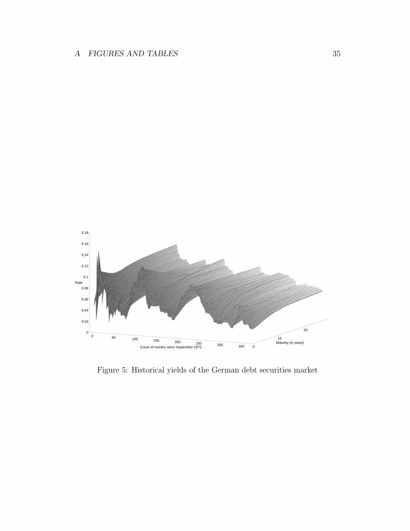
A FIGURES AND TABLES 35
Rate
0.18
0.16
0.14
0.12
0.1
0.08
0.06
0.04
0.02
0
Maturity (in years)
20
10
0Count of months since September 1972 350300250200150100500
Figure 5: Historical yields of the German debt securities market