A LARGE SCALE INTERFACE MULTIFLUID MODEL FOR

SIMULATING MULTIPHASE FLOWS

Vinesh H. GADA1*, Jebin ELIAS

1, Mohit P. TANDON

1and Simon LO

2

1 CD-adapco, Pune, Maharashtra, India2 CD-adapco, Didcot, Oxfordshire, United Kingdom

*Corresponding author, E-mail address : vinesh.gada@cd-adapco.com

ABSTRACT

The scope of the Eulerian Multiphase (EMP) model inSTAR-CCM+ is extended to simulate multi-scale two-phase �ows using Large Scale Interface (LSI) model.The LSI model provides a criteria based on local phase-distribution to distinguish between regimes characterizedby small and large scale interfaces. An appropriate clo-sure for conserved variable is speci�ed for each regime,weighted sum of which forms the closure for the interac-tion between the phases. The LSI model also allows tomodel surface tension e�ects in the vicinity of large scaleinterfaces as well. The large scale interface is treatedas a moving wall using a turbulence damping procedurenear the interface. This extended multi�uid methodologyimplemented in STAR-CCM+ is validated using severalstandard two-phase �ow problems.

NOMENCLATURE

as interfacial area densityg acceleration due to gravityk turbulent kinetic energyl interaction length scale / particle diameterp pressuret relaxation time scale~u velocity

CD drag coe�cient~F interaction forceI phase pair interactionsV volumeW weight function~FS surface tension force

α volume fractionβ k − ω model closure coe�cient∆ cell quantityκ interface curvatureµ dynamic viscosityω speci�c dissipation rateρ densityσ coe�cient of surface tensionτ shear stress

Subscriptsc, d continuous, dispersed phasep, s primary, secondary phase

fr, ir, sr �rst, interface, second regimek kth phaser relativet turbulent

D, S drag, surface-tension

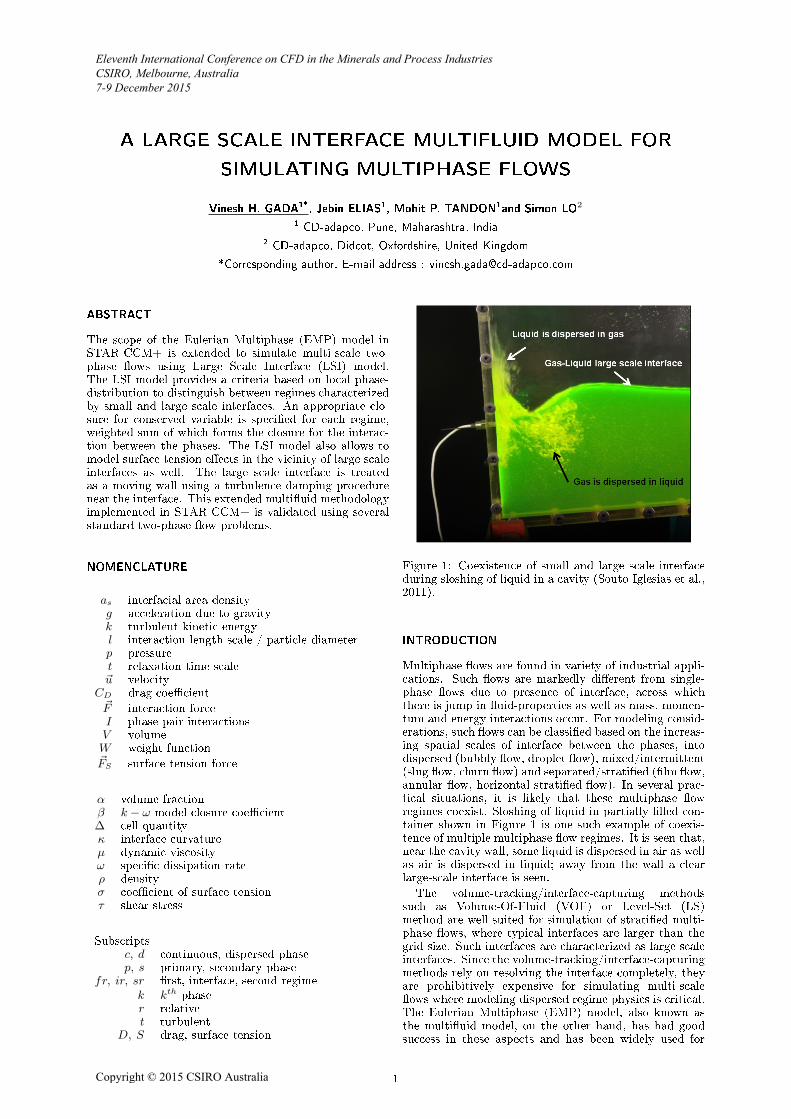
Figure 1: Coexistence of small and large scale interfaceduring sloshing of liquid in a cavity (Souto-Iglesias et al.,2011).

INTRODUCTION

Multiphase �ows are found in variety of industrial appli-cations. Such �ows are markedly di�erent from single-phase �ows due to presence of interface, across whichthere is jump in �uid-properties as well as mass, momen-tum and energy interactions occur. For modeling consid-erations, such �ows can be classi�ed based on the increas-ing spatial scales of interface between the phases, intodispersed (bubbly �ow, droplet �ow), mixed/intermittent(slug �ow, churn �ow) and separated/strati�ed (�lm �ow,annular �ow, horizontal strati�ed �ow). In several prac-tical situations, it is likely that these multiphase �owregimes coexist. Sloshing of liquid in partially �lled con-tainer shown in Figure 1 is one such example of coexis-tence of multiple multiphase �ow regimes. It is seen that,near the cavity wall, some liquid is dispersed in air as wellas air is dispersed in liquid; away from the wall a clearlarge-scale interface is seen.The volume-tracking/interface-capturing methods

such as Volume-Of-Fluid (VOF) or Level-Set (LS)method are well suited for simulation of strati�ed multi-phase �ows, where typical interfaces are larger than thegrid size. Such interfaces are characterized as large scaleinterfaces. Since the volume-tracking/interface-capturingmethods rely on resolving the interface completely, theyare prohibitively expensive for simulating multi-scale�ows where modeling dispersed regime physics is critical.The Eulerian Multiphase (EMP) model, also known asthe multi�uid model, on the other hand, has had goodsuccess in these aspects and has been widely used for

1

Eleventh International Conference on CFD in the Minerals and Process Industries CSIRO, Melbourne, Australia 7-9 December 2015

Copyright © 2015 CSIRO Australia

simulation of dispersed multiphase �ows. The EMPmodel treats each phase as inter-penetrating continuaand each phase is characterized by its own physicalproperties and velocity �eld; pressure is shared bythe phases. This generality of modeling opens up anopportunity to develop a framework for simulatingeven separated two-phase �ows using EMP model, withappropriate closures being used for Large Scale Interface(LSI) �ows.In the present work, a methodology is developed within

the multi�uid modeling framework for simulation of dis-persed as well as separated two-phase �ow. Developmentof such a method throws several challenges. Firstly, a cri-terion to classify the two-phase �ow into dispersed or sep-arated/large scale interface regime is needed. Thereafter,appropriate closure for momentum and energy shouldbe used for each regime and near the transition bound-aries, these closures should be smoothly blended for nu-merical stability. For dispersed two-phase �ow, the ef-fect of surface-tension is included in the interface drag(Tomiyama et al., 2002). However, in case of LSI regime,the surface-tension needs to be modeled explicitly. Theexistence of LSI in separated regime also needs specialmodeling of turbulence quantities in its vicinity. For ageneral case of gas-liquid �ow, the gas phase sees the in-terface as a moving wall. Thus, the turbulence needs tobe dampened in the vicinity of the large scale interface tocapture this e�ect. In this paper, a systematic approachto each of these challenges is presented in form of theLSI model, implemented in STAR-CCM+. The modelis validated on variety of separated two-phase problems:dam-break simulation, Young-Laplace law test, turbulentair-water strati�ed �ow and laminar oil-water strati�ed�ow with heat transfer.

MATHEMATICAL MODEL DESCRIPTION

Eulerian Multiphase (EMP) model treats the contribut-ing phases as interpenetrating continua coexisting in the�ow domain. Equations for conservation of mass, mo-mentum, energy and turbulence are solved for each phase(Tandon et al., 2013 and CD-adapco, 2015). The shareof the �ow domain occupied by each phase is given byits volume fraction and each phase has its own velocity,temperature �elds and physical properties. Interactionsbetween phases due to di�erences in velocity and tem-perature are taken into account via the inter-phase trans-fer terms in the transport equations; which provide theclosure to the set of equations. In the solution methoddescribed here, all the phases share a common pressure�eld.

GOVERNING EQUATIONS Considering adiabatic �ows,the main equations solved here are the conservation ofmass and momentum for each phase.

CONTINUITY

The conservation of mass for the kth phase is :

∂

∂t(αkρk) +∇ · (αkρk~uk) = 0 (1)

where αk, ρk and ~uk is volume fraction, density andvelocity of phase k, respectively. The sum of the volumefractions is equal to unity.

MOMENTUM

The conservation of momentum for the kth phase is :

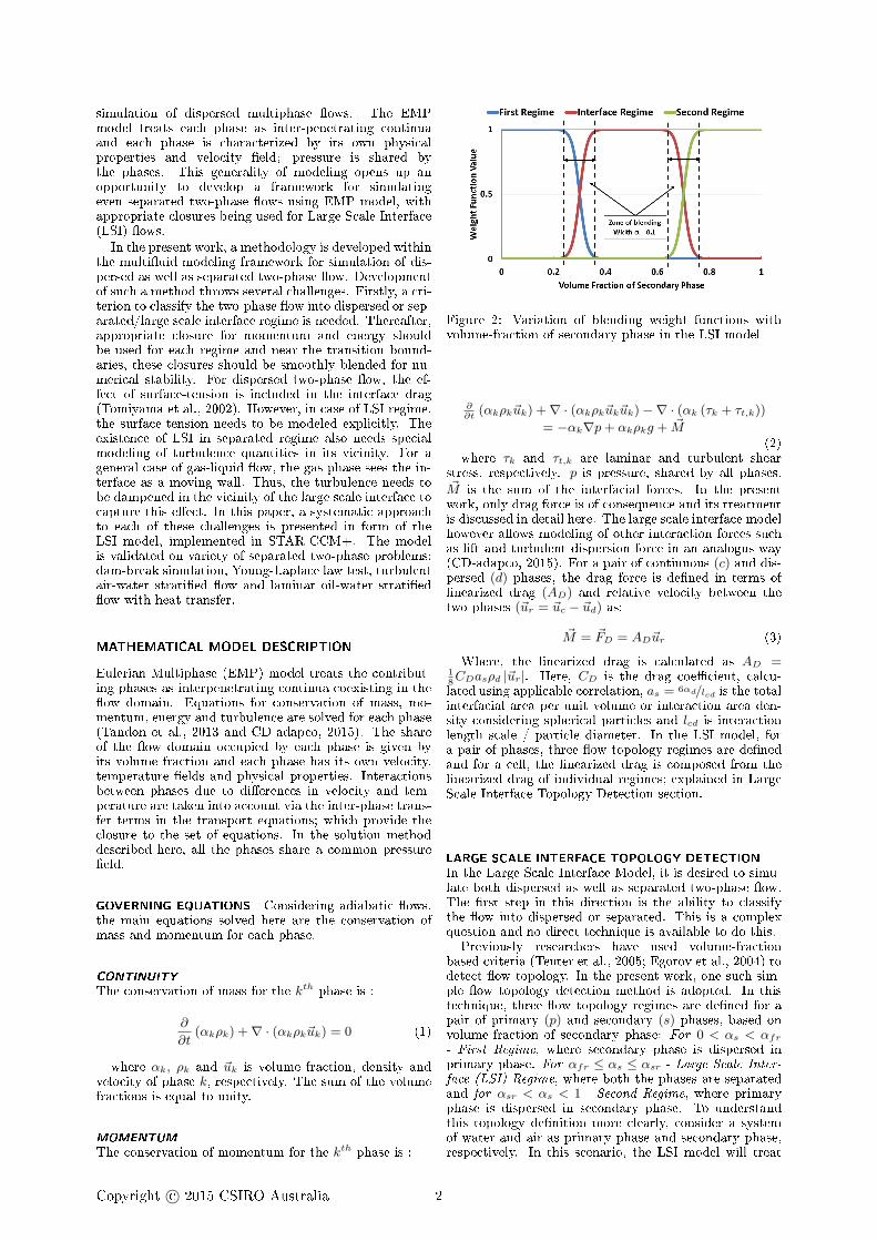
Figure 2: Variation of blending weight functions withvolume-fraction of secondary phase in the LSI model

∂∂t

(αkρk~uk) +∇ · (αkρk~uk~uk)−∇ · (αk (τk + τt,k))

= −αk∇p+ αkρkg + ~M(2)

where τk and τt,k are laminar and turbulent shearstress, respectively. p is pressure, shared by all phases.~M is the sum of the interfacial forces. In the presentwork, only drag force is of consequence and its treatmentis discussed in detail here. The large scale interface modelhowever allows modeling of other interaction forces suchas lift and turbulent dispersion force in an analogus way(CD-adapco, 2015). For a pair of continuous (c) and dis-persed (d) phases, the drag force is de�ned in terms oflinearized drag (AD) and relative velocity between thetwo phases (~ur = ~uc − ~ud) as:

~M = ~FD = AD~ur (3)

Where, the linearized drag is calculated as AD =18CDasρd |~ur|. Here, CD is the drag coe�cient, calcu-

lated using applicable correlation, as = 6αd/lcd is the totalinterfacial area per unit volume or interaction area den-sity considering spherical particles and lcd is interactionlength scale / particle diameter. In the LSI model, fora pair of phases, three �ow topology regimes are de�nedand for a cell, the linearized drag is composed from thelinearized drag of individual regimes; explained in LargeScale Interface Topology Detection section.

LARGE SCALE INTERFACE TOPOLOGY DETECTION

In the Large Scale Interface Model, it is desired to simu-late both dispersed as well as separated two-phase �ow.The �rst step in this direction is the ability to classifythe �ow into dispersed or separated. This is a complexquestion and no direct technique is available to do this.Previously researchers have used volume-fraction

based criteria (Tenter et al., 2005; Egorov et al., 2004) todetect �ow topology. In the present work, one such sim-ple �ow topology detection method is adopted. In thistechnique, three �ow topology regimes are de�ned for apair of primary (p) and secondary (s) phases, based onvolume-fraction of secondary phase: For 0 < αs < αfr- First Regime, where secondary phase is dispersed inprimary phase. For αfr ≤ αs ≤ αsr - Large Scale Inter-face (LSI) Regime, where both the phases are separatedand for αsr < αs < 1 - Second Regime, where primaryphase is dispersed in secondary phase. To understandthis topology de�nition more clearly, consider a systemof water and air as primary phase and secondary phase,respectively. In this scenario, the LSI model will treat

Copyright c© 2015 CSIRO Australia 2

bubbly �ow in the �rst regime, droplet �ow in the secondregime and separated water-air �ow in the LSI regime.The two thresholds, �rst regime terminus (αfr) and

second regime onset (αsr) gives the �exibility to controlthe extent sub-topology. αfr is the value of αs, acrosswhich the �rst regime transits to LSI regime and αsr isthe value of αs, across which the LSI regime transits tosecond regime. For the present work, their value is takenas αfr = 0.3 and αsr = 0.7.These classi�cation of regimes are enforced in every

computational cell by calculating the composite interac-tion using weighted average of linearized drag for eachregime.

I =∑

r=fr,ir,sr

[WrIr] (4)

where, I are phase-pair interactions such as lin-earized drag (AD). The weight functions for eachregime calculated as Wfr = 1/(1+exp(C(αs−αfr))),Wsr =1/(1+exp(C(αsr−αs))) and Wir = 1 − (Wfr +Wsr). Thesefunctions are plotted in Figure 2; Note that, away fromthe transition thresholds, the weight-functions reduce to0 or 1. Whereas close to transition boundaries, they varysmoothly between 0 and 1. Also, the width of the tran-sition between two regimes is close to α = 0.1. For the�rst as well as second regime the calculation of phase-pair interactions i.e. linearized drag or heat-transferare analogous to a general case of continuous-dispersedphase interaction, except for the the fact that in �rstregime, primary-phase is considered as the continuousphase and vice-versa in second regime, secondary-phase isconsidered as the continuous phase. These sub-topologyregimes therefore need, two interaction length scales, lpsand lsp for �rst and second regime, respectively. For thewater-air phases, lps and lsp refer to typical bubble anddroplet diameter, respectively. The calculation of lin-earized drag for LSI regime is discussed in following sec-tion.

LARGE SCALE INTERFACE DRAG

In the vicinity of large scale interface, the assumptionof spherical interface shape no longer is valid. Several(Frank, 2005; Coste, 2013 and Höhne & Mehlhoop, 2014)approaches have been proposed to model the drag in LSIregime. Physically, for the LSI regime, where the scale ofthe interface is nearly of the order of cell size, the largescale interface drag should lead to reduced inter-phasevelocity-slip. In the present work, method of �trubeljand Tiselj (2011) is adapted to calculate interface lin-earized drag coe�cient. This form of the interface lin-earized drag coe�cient ensures that the phase occupyinglarger volume in the cell imparts force to the other phase.The large scale interface linearized drag coe�cient is ex-pressed as:

AD,ir =1

tirαpαsρm (5)

where tir is the relaxation time-scale. In the presentwork, a low value (0.01 s) of tir is used to ensure instan-taneous equalizing of velocities of both the phases. Notethat, the value of tir can be modi�ed to change the ve-locity slip in the vicinity of large scale interface based onthe problem at hand.

LSI SURFACE TENSION MODEL

The surface tension force is an interfacial force, which ismodeled as volumetric force using the Continuum Sur-face Force (CSF) approach Brackbill et al., (1992). Fora single-velocity formulation (e.g. VOF method), the

surface tension force, more speci�cally interfacial tensionforce is calculated as:

~FS = σκδn̂ = σκ∇αp (6)

where, σ is the coe�cient of surface/interfacial tension,κ = −∇ · n̂ is the interface curvature, δ = |∇αp| is theinterfacial area density and n̂ = ∇αp/|∇αp| is the unit in-terface normal; the subscript p denotes the primary phaseof the phase-interaction. �trubelj et al., (2009) proposedthe extension of CSF model for multi�uid model by split-ting the surface-tension force among the phases occupy-ing the cell as ~FS,k = φk ~FS , where subscript k indicateskth phase and φk denotes the splitting factor of the sur-face tension force. The pressure gradient within the mul-ti�uid model is calculated by summation of momentumequations :

∑k αk∇p = ∇p =

∑k φk

~FS . At kinetic equi-librium, the pressure gradient should be equal to surfacetension force, thus :

∑k φk = 1. �trubelj et al., (2009)

showed that use of φk = αk is better than other alterna-tives, thus the surface-tension source term is in presentwork is implemented as:

~FS,k = αkσκ∇αp (7)

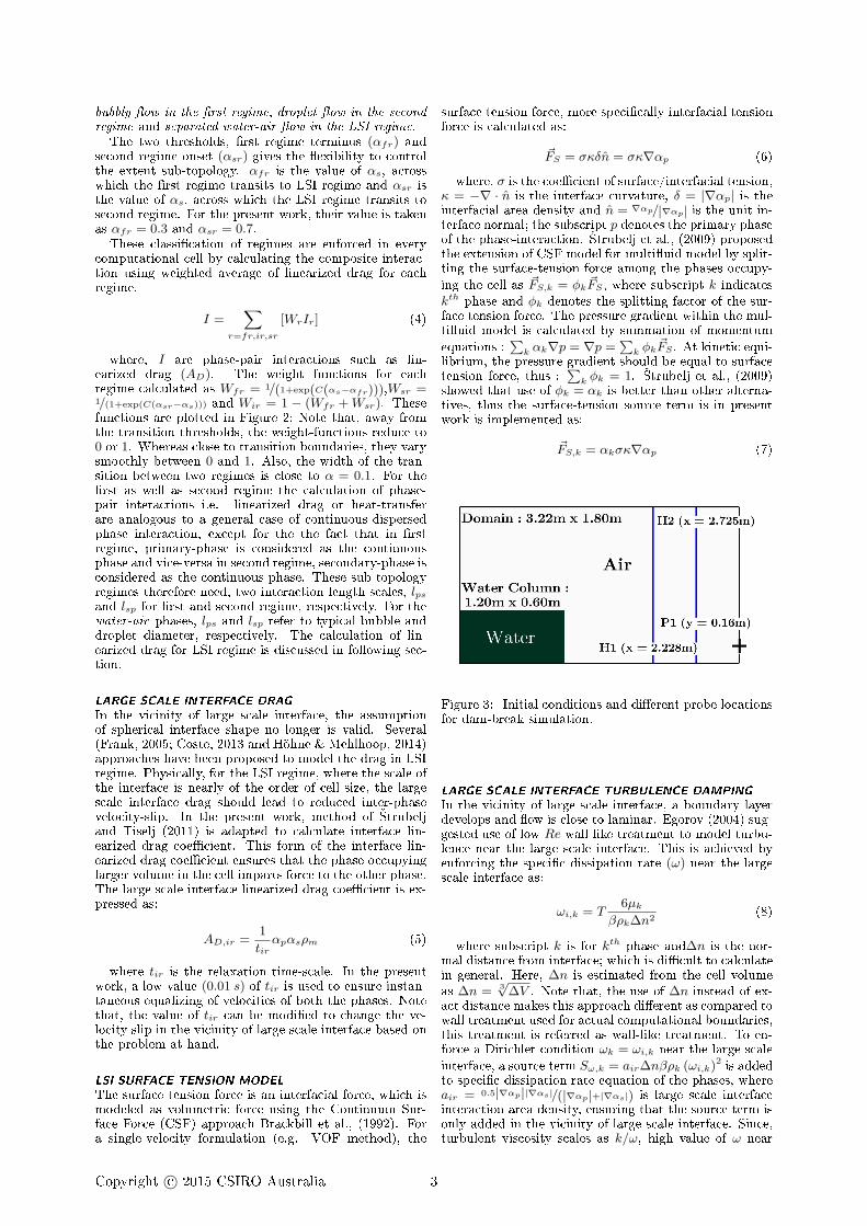
Figure 3: Initial conditions and di�erent probe locationsfor dam-break simulation.

LARGE SCALE INTERFACE TURBULENCE DAMPING

In the vicinity of large scale interface, a boundary layerdevelops and �ow is close to laminar. Egorov (2004) sug-gested use of low Re wall like treatment to model turbu-lence near the large scale interface. This is achieved byenforcing the speci�c dissipation rate (ω) near the largescale interface as:

ωi,k = T6µk

βρk∆n2(8)

where subscript k is for kth phase and∆n is the nor-mal distance from interface; which is di�cult to calculatein general. Here, ∆n is estimated from the cell volumeas ∆n = 3

√∆V . Note that, the use of ∆n instead of ex-

act distance makes this approach di�erent as compared towall treatment used for actual computational boundaries,this treatment is referred as wall-like treatment. To en-force a Dirichlet condition ωk = ωi,k near the large scaleinterface, a source term Sω,k = air∆nβρk (ωi,k)2 is addedto speci�c dissipation rate equation of the phases, whereair = 0.5|∇αp||∇αs|/(|∇αp|+|∇αs|) is large scale interfaceinteraction area density, ensuring that the source term isonly added in the vicinity of large scale interface. Since,turbulent viscosity scales as k/ω, high value of ω near

Copyright c© 2015 CSIRO Australia 3

the large scale interface leads to reduction of µt and ef-fectively leads to laminarization of �ow. The magnitudeof ω in the large scale interface region is controlled bythe turbulent damping constant T whose recommendedvalue is taken to be at least 100 as demonstrated by Lo& Tomasello (2010) for VOF method.

VALIDATION CASES

The LSI model is validated on three standard test cases;each case is selected to highlight di�erent capability of theapproach : drag formulation, turbulence damping modeland surface-tension model.

(a) τ = 0 (b) τ = 1.29

(c) τ = 3.80 (d) τ = 5.90

(e) τ = 6.80 (f) τ = 7.12

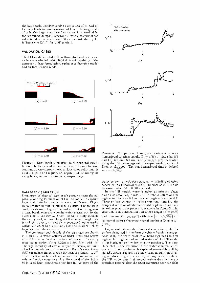
Figure 4: Dam-break simulation (a-f) temporal evolu-tion of interface visualized in the form of volume-fractioncontour. In the contour plots, a three color color-band isused to signify �rst regime, LSI regime and second regimeusing black, red and white color, respectively.

DAM BREAK SIMULATION

Simulation of classical dam-break scenario tests the ca-pability of drag formulation of the LSI model to capturelarge scale interface under transient conditions. Physi-cally, a water column con�ned to a corner of rectangularcavity as shown in Figure 3, is suddenly let o�, triggeringa dam break scenario wherein water rushes out to theother side of the cavity. Once the water body impactsthe cavity wall, it rises along it till a certain height, af-ter which it overturns and air is entrapped momentarilywithin the water body; during which the small as well aslarge scale interface co-exist.The computational details of the test case are shown

in Figure 3. A water column of width 1.2m and heightH = 0.6m is con�ned at bottom left corner of a cavityrectangular cavity of size 3.22m × 1.8m, �lled with air.The top boundary of cavity is open to atmosphere andall other boundaries are set to wall. For this case, k − ωSST turbulence model is used for both the phases. A 2nd

order TVD advection scheme is used for �ow as well asvolume-fraction equations. A uniform grid of size 144 ×80 is used here; considering the free fall velocity of the

(a)

(b)

(c)

Figure 5: Comparison of temporal variation of non-dimensional interface height (Y = y/H) at plane (a) H1and (b) H2 and (c) pressure (P = p/ρ1gH) calculatedusing the LSI model against the experimental results ofZhou et al., 1999. The non-dimensional time is de�nedas τ = t/

√H/g.

water column as velocity-scale, us =√

2gH and usingconservative estimate of grid CFL number as 0.15, stabletime-step value ∆t = 0.001s is used.In the LSI model, water is taken as primary phase

and air as secondary phase with threshold values of �rstregime terminus as 0.3 and second regime onset as 0.7.Three probes are used to collect temporal data i.e. thetemporal variation of interface height at planeH1 andH2as well as pressure at point P1, as shown in Figure 3. Thevariation of non-dimensional interface height (Y = y/H)

and pressure (P = p/ρ1gH) with time(τ = t/

√H/g)are

compared against the experimental results of Zhou et al.,(1999).

Figure 4a-f, shows the temporal evolution of the in-terface visualized in the form of volume-fraction contour.Note that, the three color color-band signi�es the �rstregime, LSI regime and second regime of the LSI modelusing black, red and white color, respectively. The plotsshow that, basic evolution of the water column, as re-ported in the experiment is captured reasonably well bythe LSI model. Figures 4d-f show that, in addition to us-ing interface drag in the vicinity of large scale interface,the LSI model uses �rst/second regime drag in the ap-propriate regions after the water overturns near the right

Copyright c© 2015 CSIRO Australia 4

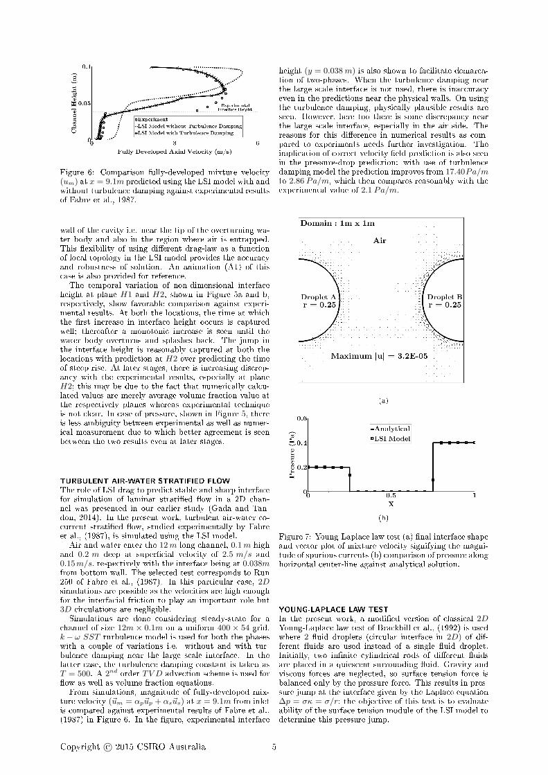
Figure 6: Comparison fully-developed mixture velocity(um) at x = 9.1m predicted using the LSI model with andwithout turbulence damping against experimental resultsof Fabre et al., 1987.

wall of the cavity i.e. near the tip of the overturning wa-ter body and also in the region where air is entrapped.This �exibility of using di�erent drag-law as a functionof local topology in the LSI model provides the accuracyand robustness of solution. An animation (A1) of thiscase is also provided for reference.The temporal variation of non-dimensional interface

height at plane H1 and H2, shown in Figure 5a and b,respectively, show favorable comparison against experi-mental results. At both the locations, the time at whichthe �rst increase in interface height occurs is capturedwell; thereafter a monotonic increase is seen until thewater body overturns and splashes back. The jump inthe interface height is reasonably captured at both thelocations with prediction at H2 over-predicting the timeof steep rise. At later stages, there is increasing discrep-ancy with the experimental results, especially at planeH2; this may be due to the fact that numerically calcu-lated values are merely average volume-fraction value atthe respectively planes whereas experimental techniqueis not clear. In case of pressure, shown in Figure 5, thereis less ambiguity between experimental as well as numer-ical measurement due to which better agreement is seenbetween the two results even at later stages.

TURBULENT AIR-WATER STRATIFIED FLOW

The role of LSI drag to predict stable and sharp interfacefor simulation of laminar strati�ed �ow in a 2D chan-nel was presented in our earlier study (Gada and Tan-don, 2014). In the present work, turbulent air-water co-current strati�ed �ow, studied experimentally by Fabreet al., (1987), is simulated using the LSI model.Air and water enter the 12m long channel, 0.1m high

and 0.2 m deep at super�cial velocity of 2.5 m/s and0.15m/s, respectively with the interface being at 0.038mfrom bottom wall. The selected test corresponds to Run250 of Fabre et al., (1987). In this particular case, 2Dsimulations are possible as the velocities are high enoughfor the interfacial friction to play an important role but3D circulations are negligible.Simulations are done considering steady-state for a

channel of size 12m × 0.1m on a uniform 400 × 54 grid.k− ω SST turbulence model is used for both the phaseswith a couple of variations i.e. without and with tur-bulence damping near the large scale interface. In thelatter case, the turbulence damping constant is taken asT = 500. A 2nd order TV D advection scheme is used for�ow as well as volume-fraction equations.From simulations, magnitude of fully-developed mix-

ture velocity (~um = αp~up + αs~us) at x = 9.1m from inletis compared against experimental results of Fabre et al.,(1987) in Figure 6. In the �gure, experimental interface

height (y = 0.038m) is also shown to facilitate demarca-tion of two-phases. When the turbulence damping nearthe large scale interface is not used, there is inaccuracyeven in the predictions near the physical walls. On usingthe turbulence damping, physically plausible results areseen. However, here too there is some discrepancy nearthe large scale interface, especially in the air side. Thereasons for this di�erence in numerical results as com-pared to experiments needs further investigation. Theimplication of correct velocity �eld prediction is also seenin the pressure-drop prediction: with use of turbulencedamping model the prediction improves from 17.40Pa/mto 2.86 Pa/m, which then compares reasonably with theexperimental value of 2.1 Pa/m.

(a)

(b)

Figure 7: Young-Laplace law test (a) �nal interface shapeand vector plot of mixture velocity signifying the magni-tude of spurious currents (b) comparison of pressure alonghorizontal center-line against analytical solution.

YOUNG-LAPLACE LAW TEST

In the present work, a modi�ed version of classical 2DYoung-Laplace law test of Brackbill et al., (1992) is usedwhere 2 �uid droplets (circular interface in 2D) of dif-ferent �uids are used instead of a single �uid droplet.Initially, two in�nite cylindrical rods of di�erent �uidsare placed in a quiescent surrounding �uid. Gravity andviscous forces are neglected, so surface tension force isbalanced only by the pressure force. This results in pres-sure jump at the interface given by the Laplace equation∆p = σκ = σ/r; the objective of this test is to evaluateability of the surface tension module of the LSI model todetermine this pressure-jump.

Copyright c© 2015 CSIRO Australia 5

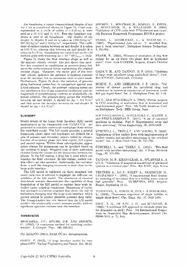
For simulation, a square computational domain of size1m × 1m is considered, shown in Figure 7a. Fluid rods,represented as a circle of radius (r = 0.25m) is initi-ated at a (0, 0.5) and (1, 0.5). Free-slip boundary con-dition is used at all boundaries. The density of thedroplet A, droplet B and air is taken as 1280.84 kg/m3,997.561kg/m3 and 1.184kg/m3, respectively. The coe�-cient of surface tension between air and droplet A is takenas 0.05 N/m, whereas that between air and droplet B istaken as 0.1N/m. Simulations are carried out on 64×64uniform grids with time-step ∆t = 10−5 till tmax = 10∆t.Figure 7a shows the �nal interface shape as well as

the mixture velocity vectors. The plot shows that inter-face has remained in equilibrium as pressure-jump bal-ances the surface-tension forces maintaining the originalcircular shape. Moreover, the vector plot of the mix-ture velocity indicates the presence of spurious currentsnear the interface but its maximum value is quite small.Furthermore, Figure 7b shows the variation of pressurealong horizontal center-line, in comparison against ana-lytical solution. Clearly, the pressure variation across thetwo interfaces is free of any numerical oscillations and themagnitude of pressure-jump con�rms to analytically ob-tained solution, the pressure-jump across the interfacebetween air and droplet A should be ∆p = 0.2 N/m2

and that across the interface between air and droplet Bshould be ∆p = 0.4N/m2.

SUMMARY

Model details of the Large Scale Interface (LSI) modelimplemented in the commercial code STAR-CCM+ arepresented to simulate multi-scale multiphase �ows withinthe multi�uid model. The LSI model provides a generalframework where three sub-topologies are de�ned for apair of primary and secondary phases, based on volume-fraction of secondary phase into �rst regime, LSI regimeand second regime. Within these sub-topologies, appro-priate closure for momentum can be speci�ed based onthe problem at hand. Weighted sum of these individualclosures forms the closure for the interaction between thephases. In the LSI regime, a drag law is used which canequalize the �uid velocities. In this regime, surface ten-sion e�ects are also modeled. Additionally, for turbulent�ows, a wall like damping treatment is done close to thelarge scale interface.The LSI model is validated on three standard test

cases; each case is selected to highlight the di�erent ca-pabilities of the LSI model. The simulation of classicaldam-break scenario demonstrates the capability of dragformulation of the LSI model to capture large scale in-terface under transient conditions. Simulation of turbu-lent air-water co-current strati�ed �ow shows the role ofturbulence damping near the large scale interface, whichproved critical to predict plausible pressure-drop value.The Young-Laplace law test showed that the LSI modelpredicts the analytically correct pressure pro�le, withoutsigni�cant spurious currents near the interface.

REFERENCES

BRACKBILL, J.U., KOTHE, D.B. AND ZEMACH,C., (1992), �A continuum method for modeling surfacetension�. J. Comput. Phys. 100, 335-354.

CD-ADAPCO (2015), STAR-CCM+ documentation.

COSTE, P. (2013), �A large interface model for two-phase CFD�, Nuclear Engineering and Design, 255, 38-50.

EGOROV, Y., BOUCKER, M., MARTIN, A., PIGNY,S., SCHEUERER, M., & WILLEMSEN, S. (2004).�Validation of CFD codes with PTS-relevant test cases�,5th Euratom Framework Programme ECORA project.

FABRE, J., MASBERNAT, L., & SUZANNE, C.,(1987). �Experimental data set no. 7: strati�ed �ow,part i: local structure�, Multiphase Science Technology,3, 285-301.

FRANK, T., (2005), �Numerical simulation of slug �owregime for an air-water two-phase �ow in horizontalpipes�. Proc. 11th NURETH, Avignon, France, October2-6.

GADA V. H., AND TANDON, M. P. (2014), �Modelingof large scale interfaces using multi-�uid theory�, Proc.2nd ICNMMF, Darmstadt, Germany.

HÖHNE, T., AND MEHLHOOP, J. P. (2014)., �Val-idation of closure models for interfacial drag andturbulence in numerical simulations of horizontal strati-�ed gas�liquid �ows�, Int. J. Multiphase Flow, 62, 1-16.

LO, S., AND TOMASELLO, A. (2010), �Recent progressin CFD modelling of multiphase �ow in horizontal andnear-horizontal pipes�. Proc. 7th North American Conf.on Multiphase. Tech., BHR Group, June.

SOUTO-IGLESIAS A., BOTIA-VERA E., MARTÍN A.and PÉREZ-ARRIBAS F., (2011), �A set of canonicalproblems in sloshing. Part 0: Experimental setup anddata processing�, Ocean Engineering, 38, 1823-1830.

�TRUBELJ, L., TISELJ, I., AND MAVKO, B. (2009).�Simulations of free surface �ows with implementation ofsurface tension and interface sharpening in the two-�uidmodel�. Int. J. Heat Fluid Flow, 30, 741-750.

�TRUBELJ, L. and TISELJ, I., (2011), �Two-�uidmodel with interface sharpening�, Int. J. Num. MethodsEngg., 85, 575-590.

TANDON, M. P., KHANOLKAR, A., SPLAWSKI A., &LO, S., �Validation of numerical simulations of gas-liquidsystems in a vertical pipe�, Proc. 8th ICMF, Jeju, Korea

TENTNER A., LO S., IOILEV A., SAMIGULIN M.,USTINENKO V., (2005), �Computational �uid dynam-ics modeling of two-phase �ow in a boiling water reactorfuel assembly�, Proc. MCSRPNBA, ANS, Avignon,France, September 12-15.

TOMIYAMA, A., TAMAI, H., ZUN, I., & HOSOKAWA,S., (2002), �Transverse migration of single bubbles insimple shear �ows�, Che. Engg. Sci., 57, 1849-1858.

ZHOU, Z. Q., DE KAT, J. O., and BUCHNER, B.(1999), �A nonlinear 3-D approach to simulate green wa-ter dynamics on deck�, Proc. 7th International Sympo-sium on Numerical Ship Hydrodynamics, Report (No.82000-NSH, p. 7), July.

Copyright c© 2015 CSIRO Australia 6