Scholars' Mine Scholars' Mine

Masters Theses Student Theses and Dissertations

1971

A hybrid computer solution of the swing equation A hybrid computer solution of the swing equation

Donald Wayne Shaw

Follow this and additional works at: https://scholarsmine.mst.edu/masters_theses

Part of the Electrical and Computer Engineering Commons

Department: Department:

Recommended Citation Recommended Citation Shaw, Donald Wayne, "A hybrid computer solution of the swing equation" (1971). Masters Theses. 7222. https://scholarsmine.mst.edu/masters_theses/7222

This thesis is brought to you by Scholars' Mine, a service of the Missouri S&T Library and Learning Resources. This work is protected by U. S. Copyright Law. Unauthorized use including reproduction for redistribution requires the permission of the copyright holder. For more information, please contact scholarsmine@mst.edu.

A HYBRID COMPUTER SOLUTION OF THE SWING EQUATION

BY

DONALD WAYNE SHAW, 1947-

A THESIS

Presented to the Faculty of the Graduate School of the

UNIVERSITY OF MISSOURI - ROLLA

In Partial Fulfillment of the Requirements for the Degree

MASTER OF SCIENCE IN ELECTRICAL ENGINEERING

T2544 c.l

1971 72 pages

1.94226

ABSTRACT

Models for the governor and exciter control systems

are presented and the development of a hybrid computing

system including these models is described. A technique

for including the governor and exciter effects into the

solution of the power system swing equation is also

discussed. A hybrid computing system consisting of an

ii

sec 650 digital computer, hybrid interface, and an EAI-TR-48

analog computer is used to study five test cases. The test

cases involve basically the same example system with

different values for fault clearing times and machine

inertias. The results of each test case are briefly dis­

cussed with relevance to the importance of the inclusion

of the control system effects. The advantages and dis­

advantages of a hybrid computing system are also discussed.

PREFACE

In the past decade, the power industry has become

increasingly dependent upon the use of digital computers

in the solution of many power system problems. The

widespread use of general purpose digital computers has

allowed the power system engineer to utilize more detailed

system representations for such studies as load flow and

transient stability. The inclusion of the governor and

exciter control system effects into transient stability

analysis is a perfect example of such added detail.

iii

Since the digital computer is a readily available

tool, the inclusion of the control system effects gener­

ally takes the form of a digital solution of the equations

describing the performance of the systems. The possibility

of using an analog computer for simulating the control

systems and a digital computer for solution of the

stability equations has not been considered. In order to

insure that a worthwhile technique does not go unnoticed,

this work will investigate the use of a hybrid computing

system to solve the transient stability problem.

The author would like to recognize Dr. J. D. Morgan

as the individual whose intelligence sparked the theme

of this thesis and also as the one whose guidance has

influenced it from its beginning. The author would also

like to thank Mr. George Rhine for his much needed

assistance and cooperation in the preparation of both the

digital software and hybrid hardware used in the hybrid

computing system. Finally, the author would like to

thank his wife, for not only the traditional moral support

but also for her direct contribution in the preparation

of the digital programs.

iv

TABLE OF CONTENTS

ABSTRACT

PREFACE

LIST OF ILLUSTRATIONS

LIST OF TABLES

I. INTRODUCTION

II. REVIEW OF THE LITERATURE

III. COMPONENTS OF THE HYBRID SYSTEM

A. Stability and the Swing Equation

B. The Governor Control System

C. The Voltage Control System

IV. THE HYBRID COMPUTING SYSTEM

V. EXAMPLE STUDIES

A. The Basic System

B. Test Cases

1. Case 1

2. Case 2

3. Case 3

4 • Case 4

5. Case 5

VI. DISCUSSION OF RESULTS

BIBLIOGRAPHY

VITA

v

Page

ii

iii

vi

vii

1

3

9

9

17

24

31

44

44

50

50

52

52

55

57

60

63

65

Figure

III-1

III-2

III-3

III-4

III-5

III-6

III-7

III-8

IV-1

IV-2

V-1

V-2

V-3

V-4

V-5

LIST OF ILLUSTRATIONS

An Unstable System

Multi-Machine Power System Representation

Governor Control System Block Diagram

Analog Simulation of Governor Control System

Control System Response to a Step Input

Synchronous Machine Model

Voltage Control System Block Diagram

Analog Simulation of Voltage Control System

Comparison of SCC 650 and IBM 360 Results

Simplified Block Diagram of Hybrid Computing System

Case 1 Swing Curves

Case 2 Swing Curves

Case 3 Swing Curves

Case 4 Swing Curves

Case 5 Swing Curves

vi

Page

11

15

20

22

23

25

28

30

38

40

51

53

54

56

58

Table

III-1

III-2

IV-1

V-1

V-2

LIST OF TABLES

Governor Control System Parameters

Exciter Control System Parameters

Simplified Flow Table for Digital Programs

Data for Basic System

Element Assignments and Potentiometer Settings

vii

Page

21

29

37

45

47

I. INTRODUCTION

For many years the complexity of electric power

systems necessitated the use of several simplifying

assumptions in order to implement an analysis technique.

With the advent of the general purpose digital computer,

many of these assumptions were no longer necessary.

Two of the most commonly used assumptions in

stability studies were constant voltage behind transient

reactance and constant power input. The accuracy of these

assumptions depends almost entirely upon the response times

of the governor and exciter control systems. In the

past, the response times of these systems were so long

compared to the transient analysis time that the assump­

tions concerning them were valid. However, in the last

ten to fifteen years, improvements in design have shortened

the response times of both of these systems, particularly

the exciter control system. With short response times,

the presence of the control systems has an appreciable

effect on the results of transient stability studies.

Therefore, in order for a transient stability study to

be complete, these systems must be included in the analysis.

The inclusion of the effects of the governor and

exciter control systems has concerned many researchers,

and many papers, such as the ones by Lokay and Bolger [1]

l

and Schleif, Hawkins, Martin and Hattan [2], have been

published. None of these efforts, however, has included

the use of an analog computer for modeling the voltage

and governor control systems in a hybrid manner. One of

the basic reasons for not using a hybrid approach is that

more computer hardware is needed. Not only are the analog

and digital computers needed, but also a hybrid interface.

From this point of view it is not difficult to see why

researchers preferred to use only the digital computer

with a digital approximation of the response of the control

systems. In doing this, however, the merits of a hybrid

computer approach were passed over. Perhaps such merits

do not exist and on the other hand, perhaps they exceed

those of a purely digital approach. In any case, the

hybrid approach warrants consideration. It is the purpose

of this research to investigate the practicality of a

hybrid computing system for use in stability studies.

2

II. REVIEW OF THE LITERATURE

The problem of power system stability is not a new

one. Perhaps one of the first stability problems elec­

trical engineers had to deal with was that of hunting.

Hunting can be described as small oscillations of the

speed of a machine about its synchronous speed. It may

be caused by changes in load, changes in excitation, or

by driving a synchronous generator with a pulsating torque

such as that produced by a steam or diesel engine. In

certain cases, if the frequency of the pulsating torque

is coincident with a natural frequency of the system, a

resxnant condition may develop which tends to make the

hunting worse, and can even result in loss of

synchronism.

The problem of hunting, however, was brought under

control by the use of damper windings introduced by

LaBlance and Lamme, and by 1910 it was virtually eliminated

by the replacement of steam engines by steam turbines and

water power.

The use of water power though brought about a new

stability problem. Since the generating station was

generally far from major loads, long distance power trans­

mission was necessary. Long transmission lines are

expensive to build, so for economic reasons it is desirable

to have them carry as much power as possible. It can be

3

shown that there is a maximum limit on the power which a

given line can carry and still maintain synchronism between

the machines at opposite ends of the line. Unfortunately,

the closer a line is operated to this maximum, the more

susceptible fue system is to transient instability.

Another problem, similar to the previous one, is

that of power interchange between two generating areas.

In most cases the tie line connecting the two areas is

designed to carry only a small percentage of the total

capacity of either area. As a consequence of this design,

whenever either system sustains a serious disturbance, the

amount of synchronizing power which can flow is not suffi­

cient to maintain stability. A natural solution to this

problem would be to design the tie line such that it could

carry a large amount of synchronizing power.

Indeed, this could be done, but under normal opera­

tion the line would not be used near its maximum limit.

Therefore, the consideration of economy again enters the

picture.

It would seem then that the basic problems of power

system stability reduce to a trade-off between economy of

operation and stability of operation. Any improvement in

the stability of a system not accompanied by a substantial

cost would therefore be of much interest.

Real interest in power system stability began in the

decade 1910 - 1920, and many methods of analysis, such as

regulation studies, circle diagrams, synchronous machine

4

theory, and symmetrical components were developed during

that time. Since 1920 power system stability has been

of major interest to many researchers.

One of the first efforts at analysis was made by

R. H. Park and E. H. Bancker [3]. These men are credited

with the development of the equal area criterion, which is

used as a measure of stability. This technique of deter­

mining the stability of a system is easily applied as an

instructive device and it also gives an intuitive feel

for the stability problem. Unfortunately, the method is

not directly applicable to more than a two machine system.

The method also neglects the effects of governor and

exciter responses, even though it was known that parti­

cularly the exciter system had an important effect on

stability.

Perhaps the next significant work was that of

Selden B. Crary [4]. Crary extended the work of Park and

Bancker and also discussed multi-machine systems, long

distance power transmission, generator characteristics,

system design, and high speed circuit breakers. Crary's

multi-machine approach is based mainly on the use of

either delta-wye transformations or an ac network analyzer

to obtain the driving point and transfer impedances which

are used in the swing equation solution. The step by

step solution of the swing equation is discussed by Crary

and he also presents a method for including the effects

5

of the excitation system response into the swing equa­

tion solution.

E. W. Kimbark published one of the next significant

works on power system stability [5]. Kimbark explains

what the stability problem is and then develops and

explains in detail the solution of the swing equation

using the step by step method. He then presents a method

for applying the step by step solution to a multi-machine

system by the use of an admittance network. This work

also contains excellent discussions of the equal area

criterion, the two machine system, faulted three phase

networks, and typical stability studies.

By the early 1950's, certain techniques of deter­

mining the transient stability of a power system were

well developed. It was known for a number of years that

the governor and exciter control systems tended to

improve the results of transient stability studies in most

cases. However, the inclusion of these effects was

generally omitted from the analysis for the sake of

simplicity, and with no significant loss of accuracy,

since for first swing calculations, the approximations

of constant voltage behind transient reactance and con­

stant power input are fairly good. In addition, these

approximations result in conservative stability results.

With the advent of the general purpose digital com­

puter in the mid 1950's, the inclusion of the governor

6

and exciter characteristics into the solution of the swing

equation was inevitable. Accompanying the digital computer

were new iterative techniques for solving the load flow

and transient stability problems.

One of the first comprehensive works concerning

digital computer techniques was published by Glenn W. Stagg

and A. H. El-Abiad [6]. Stagg and El-Abiad present

algorithms for the formation of network matrices, methods

of numerical solution of differential equations, load flow

studies, and transient stability studies. In their work,

they also deal with the analysis of the transient stability

problem. Their approach is to combine the solution of

the algebraic equations of the network with the numerical

solution of the differential equations which describe the

performance of the machines. The authors discuss both the

Euler and Runge-Kutta methods as applied to the solution

of the differential equations of the system. They also

present a method for including the governor and exciter

responses into the iterative solution of the swing

equation.

One method for including the effects of the governor

and exciter systems is to solve the control system equa­

tions simultaneously with those of the swing equation.

This results in a digital approximation to the perfor­

mance of the control systems. The inclusion of these

effects has been studied and in a paper published by

H. E. Lokay and R. L. Bolger [1]. In their work, Lokay

7

and Bolger studied the effect of increasingly detailed

turbine-generator representations on stability limits.

The results of their work confirmed that the conventional

approximations for the solution of the swing equation were

valid. Moreover, their results showed that the excita­

tion control system has a greater influence on stability

than the speed-governor system.

Since 1960 several papers have been published

concerning the effects of the governor and exciter repre­

sentations on the stability of a power system. For the

interested reader, references [2], [7], [8], and [9] in

the bibliography will provide much information on this

topic.

Such is the present state of the art in the transient

stability analysis of power systems. Much has been

accomplished, but surely much more needs to be done. It

is the purpose of this research to contribute to the

present knowledge by investigating the merits of a hybrid

computer approach.

8

III. COMPONENTS OF THE HYBRID SYSTEM

A. Stability and the Swing Equation

In order to determine if a given power system is

stable under transient conditions, a stability criterion

is needed. According to the "American Standard Definitions

of Electrical Terms" [10], stability may be defined as

follows.

"Stability, when used with reference to a power system, is that attribute of the system or part of the syste~ which enables it to develop restoring forces between the elements thereof, equal to or greater than the disturbing forces so as to restore a state of equilibrium between the elements."

For the purposes of this paper, the above definition

is taken to mean that under transient conditions, the

stability of a system under study may be determined by

observing the variation of the machine angles of the system

from a fixed reference. If the absolute value of any

machine angle with respect to the fixed reference continues

to increase during the analysis time, then that machine is

considered to lose synchronism with the rest of the system

9

and the entire system is considered unstable. Mathematically

this amounts to stating that the derivative of each curve

of machine angle versus time must at some point in the

analysis go to zero for the system to be stable. However,

using this definition, a system could still go unstable

10

and satlsfy the derivative requirement. It could not,

however, be stable without each derivative going to zero.

For example, consider the curves of Figure III-1. Each

curve at one point or another has a derivative of zero,

yet the system is unstable.

In order to use the above criterion to determine if

a system is stable, the curves of machine angle versus

time are needed. These curves may be obtained by the

solution of the swing equation. Since the swing equation

is the foundation upon which the determination of system

stability lies, a review of its origin seems in order [5,10].

Ignoring friction, windage and rotational losses,

the difference between the shaft torque, Ts, and the elec­

tromagnetic torque, Te' on the shaft of a generator may

be given as

T = T - T a s e (III-1)

where T is an accelerating torque which is positive when a

Ts is greater than Te. Note that in steady state, T = T s e

and T is zero. a Recall, however, that P = Tw; therefore,

p = P. a ln

is also a valid expression.

(III-2)

Pa is accelerating power, P. ln

is shaft power input, and Pu is the electric power developed.

Also recall from the mechanics of rotating objects that

T = Ia, and also that Iw is the angular momentum of a

rotating machine. The quantity Iw, though, is recognized

en LU LU a:::: (!) LU ~

_J

<t: u -a:::: 1-u LU _J LU

z:

MACHINE

MACHINE

TIME IN SECONDS

Figure III-1. An Unstable System

11

REFERENCE

12

as M, the inertia constant of a rotating machine. Note that

the value of M changes as the angular velocity changes.

However, assuming w is relatively constant during the

transient analysis time, M may be considered constant.

Common units for M are megajoule-second/electrical degree.

Pa' then, may be expressed as

P = T w = Iaw = Ma a a (III-3)

The angular acceleration, a, may be expressed in terms of 8,

an angle which is measured from a non-rotating reference.

(III-4)

The final objective, however, is an equation involving

o, the synchronous machine angle, which is measured from a

reference rotating at synchronous speed.

the synchronous speed ws' o is given as

or

o = e - w t s

In terms of 8, and

(III-5)

8 = w t + o (III-6) s

Differentiating (III-6) twice with respect to time,

(III-7)

Or, a may be written as

(III-8)

13

Therefore, since p = Ma, then a

p M d 2 cS = dt2 a (III-9)

and from Pa = P. - p ~n u (III-10)

M d 2 o P. p

dt2 = -

~n u (III-11)

Equation (III-11) is the swing equation. The solution

of this second order differential equation yields the

values of cS as a function of time and can therefore be

used to plot curves of cS versus time.

In order to solve Equation (III-11) , a step by step

method is used. Two basic assumptions are made. These

assumptions, as listed by Stevenson [11] are:

1. The accelerating power Pa' computed at the

beginning of an interval is constant from the

middle of the preceding interval to the middle

of the interval considered.

2. The angular velocity, w, is a constant through-

out any interval, at the value computed for the

middle of the interval.

Between midpoints of any two intervals of the step

by step solution, say N - 3/2 and N - 1/2, where N is the

interval under present consideration, the change in speed,

IJ.w', is given by

14

p a (N - 1) t:.t ,

M ( III-12)

where w' = w - w and t:.t is the time interval. The change s

in o over any time interval can be easily calculated as

the product of the relative angular speed, w', and the time

interval. The change in o, t:.o, may therefore be written

as

' t:.oN = t:.twN-1/2 = 0N - 0N-l (III-13)

An identical equation may be written for the N-1 interval.

I

t:.oN-1 = t:.twN-3/2 = 0N-l - 0N-2 (III-14)

Subtracting Equation (III-14} from (III-13} ,

' t:.oN - t:.oN-1 = WN-1/2 - WN-3/2

or, from Equation (III-12),

p t:.o = t:.o + a(N-1) (t:.t)2

N N-1 M (III-15)

The step by step solution of the swing equation may

therefore be summarized in the steps below.

1. Calculate P from P = P. - P . a a ~n u

2. Pa(N-1)

calculate t:.o from t:.oN = t:.o(N-l) + M (t:.t) 2

4. Repeat above steps for each machine until

analysis is complete.

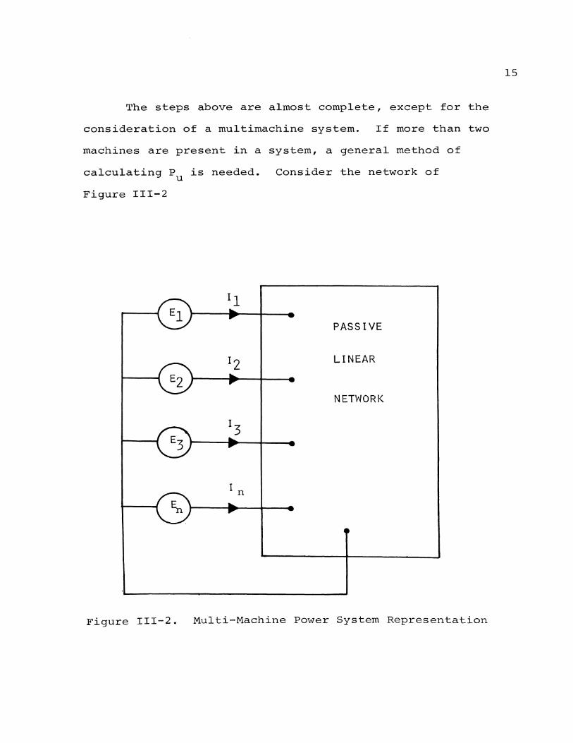
The steps above are almost complete, except for the

consideration of a rnultimachine system. If more than two

machines are present in a system, a general method of

calculating Pu is needed. Consider the network of

Figure III-2

PASSIVE

LINEAR

NETWORK

Figure III-2. Multi-Machine Power System Representation

15

16

It can be shown that the real power input to the network

from any machine n of an m machine system is given by

' [5] (III-16)

where Ynk~nk is a complex admittance term of the network

and EJon and E~k are voltages behind transient

reactance.

The angles of E and Ek n are the same machine angles

discussed in the swing equation solution. Multimachine

systems may be solved then by using Equation (III-16) to

calculate Pu used in Equation (III-10) . Note that the n

machine angles used in Equation (III-16) will continually

change with the progression of the solution.

In brief review, then, the solution of the swing

equations of the system will provide the information

necessary to plot swing curves, or curves of 6 versus

time. By using the stability criterion stated before,

the swing curves will determine whether or not the system

is stable. At this point it is evident that this is one

technique of determining stability. However, the inclusion

of the governor and exciter effects into the analysis has

not been considered. Since familiarity with these systems

is necessary before they can be included in the solution

of the swing equation, these control systems are discussed

in the following sections.

B. The Governor Control System

When the steam engine was first used as a prime

mover for generators, the angular speed of the machine

was controlled by the fly-ball type governor of the steam

engine. Since that time, governor controls have become

somewhat more complex, but their function has remained

basically the same, that of maintaining the required power

input at the proper angular velocity. Note that the

governor responds to a change in speed, which usually

results from a change in demand on the generator. There

are various types of governors which respond to signals

other than a change in speed; however, they will not be

considered. In order to understand qualitatively how

the governor can influence the stability of a system under­

going a fault or open circuit, consider the following.

Suppose that a disturbance on a given system causes

the power output of a certain machine to decrease below

its value before the disturbance. Since the power input

cannot change instantaneously, there is an unbalance

between output power and input power. Energy is being

absorbed by the machine. The only way the machine can

store this excess energy is to spin faster. This it

does and in so doing increases its output frequency and

moves away from the reference frequency. If the frequency

deviation is too severe, the machine will lose synchronism

with the rest of the system. Now, since it has already

17

been established that the governor responds to deviations

in speed, it is reasonable to .expect that when the machine

speeds up the governor will respond in such a manner as

to decrease the speed. The governor system, in order to

reduce the speed, reduces the power input to the prime

mover. This helps to balance the input and output powers

and decreases the absorption of energy by the generator.

As can be seen from inspection of Equations (III-2)

and (III-15), a decrease in power input due to th.e governor

response tends to decrease the value of ~o. In general,

the smaller the change in the machine angles, the more

stable the system will be. In any case, the governor

response will definitely affect the results of a stability

study. Since the governor control system does influence

stability, its inclusion in the swing equation solution

is required. This requirement should, however, be

reviewed, depending upon how fast a given control system

can respond. If the response is too slow to appreciably

change the power input before the end of the transient

analysis, then, including the effect of governor control

adds nothing but complexity to the solution. Assume,

however, that such is not the case and it is desirable to

include the effects of the governor control system.

In order to include the governor system, it must

first be modeled. Fortunately, much work has been done

in developing suitable models, and several different

18

models may be used. However, the basic factor in the

choice of a model for this work was the availability of

reliable data. On this basis, the model shown in Fig-

ure III-3 was chosen. Parameter values for this system

were available from a previous work [1] and were therefore

assumed correct. With the block diagram model and

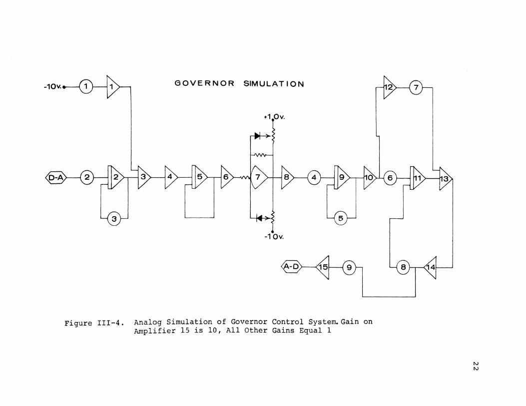
constants established, the conversion to analog simulation

was easily accomplished. The analog program is shown in

Figure III-4. Table III-1 lists the parameter values

which were used.

The system of Figure III-4 was patched on the TR-48

analog computer and found to respond satisfactorily to

various inputs. These initial tests also revealed that

the governor system chosen had a relatively quick response

to a step input. As can be seen in Figure III-5, the

governor system responds very quickly compared to the

voltage control system. Such a quick response would, of

course, aid stability. The author, however, had not

expected the governor to enter quite so prominently into

the transient analysis of the swing equation.

Having satisfactorily responded to test situations,

the governor simulation was ready for the hybrid system.

The voltage control system, however, still required

modeling, simulation, and testing before the hybrid system

could be completed. The voltage control system is the

subject of the next section.

19

GOVERNOR CONTROL SYSTEM BLOCK DIAGRAM

1

w' DEVIATION FROM SYNCHRONOUS VELOCITY

Figure III-3. Governor Control System Block Diagram

N 0

21

PARAMETER DESCRIPTION

K1 Control System Gain

T1 Control System Time Constant

T3 Servo Valve Time Constant

P Maximum Power Limit max

P . Minimum Power Limit m~n

PARAMETER VALUES

Kl = 0.219

Tl = 0.15 seconds

T3 = 0.05 seconds

T4 = 0.1 seconds

T5 = 10.0 seconds

K2 = 0.23

p = 6.75 per unit max

p min = o.o per unit

Table III-1. Governor Control System Parameters

-10V.

Figure III-4.

GOVERNOR SIMULATION

+1 Ov.

-1 ov.

Analog Simulation of Governor Control Syste~Gain on Amplifier 15 is 10, All Other Gains Equal 1

1.4

1--:z: =:;) 0 6 a:::' LLJ a..

0.2

'------- GOVERNOR CONTROL SYSTEM

O.OL-------~~------~~------~--------~--------~ 5.0 10.0 15.0 20.0 25.0

TIME IN SECONDS

Figure III-5. Control System Response to a Step Input

N w

C. The Voltage Control System

The purpose of a voltage control system on a large

generator is to maintain a desired voltage at the

terminals of the machine. The terminal voltage is

affected by changes in terminal current and therefore

the excitation must be changed whenever the current

changes in order to maintain a constant terminal voltage.

This can be easily deduced by examination of the model of

a synchronous generator given in Figure III-6.

Suppose that the generator is providing no load,

that is, I is equal to zero. Immediately from Kirchhoff's

voltage law it can be seen that VT is equal to Ein for any

given excitation. However, suppose the generator is

loaded and I is not zero. Kirchhoff's voltage law reveals

that VT is no longer equal to Ein' their difference being

the voltage drop across xd'. For a change in load, then,

the excitation must change in order to change the value

of E. such that the magnitude of VT remains constant. A ~n

reasonable model of such a system could be made by sub-

tracting the terminal voltage from a reference value and

generating an error signal which changes the excitation.

other techniques of changing the excitation may also be

used, but a system using a voltage error as a drive was

preferred for this work. Before proceeding to an actual

model of a voltage control system, consider how such a

system can influence stability.

24

25

I

Figure III-6. Synchronous Machine Model

Given the manner in which a voltage control system

responds, look again at the solution of the swing equa-

tion. Suppose that a disturbance on a power system causes

the terminal voltage on a given machine to decrease. The

control system would receive an error signal which would

tend to increase E. ~n

Now, examination of Equation (III-16)

reveals that the electrical power output will increase.

Since P increases, then P will decrease and the result-u a

ing change in the machine angle for a particular iteration

will be smaller. Taken over many iterations, with a

steadily increasing response from the exciter, the decrease

in the value of P is enough to significantly influence a

the stability of a system. As with the governor system,

the exciter must be included in the solution if the

analysis is to be complete. Again, depending upon the

comparison between the analysis time and response time,

inclusion of the exciter control system may add nothing;

however, most exciters respond quickly enough that they

require inclusion for accurate results.

In order to include the voltage control system in

the solution of the swing equation, it must first be

modeled.

The particular model for a given type of exciter

has been established by the IEEE Committee on Computer

Representation of Exciter Control Systems [12]. Since

the choice of systems for this research was arbitrary,

26

the selection of a Type 1 - Continuously Acting Regulator

was made. Figure III-7 shows the Type 1 block diagram

with magnetic saturation and the regulator stabilizer

loop omitted. Space limitations on the TR-48 analog

computer made it necessary to neglect magnetic saturation

and parameter values eliminated the stabilizer loop. As

with the governor system, once the model was chosen and

parameters available, the system was converted to an

analog simulation. The voltage control simulation is

shown in Figure III-8 and the parameter values are listed

in Table III-2. The simulation was subjected to various

tests to determine if it would respond correctly to

different inputs. The response of the simulation to a

step input is shown in Figure III-5. As with the governor

simulation, once the system had been tested it was ready

for the hybrid system. Actually, in the case of the

voltage control system, two identical systems were built

so that voltage control effects on two machines could

be included in an example study. With these two systems

and the governor control system working properly, only a

few difficulties remained before a working hybrid system

could be built. The method of including the control system

effects and the problems involved are discussed in the

next chapter.

27

VOLTAGE CONTROL SYSTEM BLOCK DIAGRAM

VRMAX +

KA f 1 1 + STA KE + STE

VRMIN

Figure III-7. Voltage Control System Block Diagram

Kv

1 + STDO

VT

1\J 00

v Tmin

vref

TR

KA

TA

v Rmax

VR . m~n

=

=

=

=

=

PARAMETER DESCRIPTION

Regulator Input Filter Time Constant

Regulator Gain

Regulator Amplifier Time Constant

Maximum Value of Regulator Output Voltage

Minimum Value of Regulator Output Voltage

Regulator Reference Voltage Setting

Exciter Constant Related to Self Excited Field

Exciter Time Constant

Constant Relating Field Voltage to Terminal Voltage

Open Circuit Time Constant

PARAMETER VALUES

0.05 seconds KE = 0.145

5.0 TE = 0.09 seconds

0.88 seconds Kv = 1.0

1.0 per unit TDO = 5.0 seconds

1.0 per unit

Table III-2. Exciter Control System Parameters

29

EXCITER SIMULATION

-10~

-10v.

Figure III-8. Analog Simulation of Voltage Control System

All Amplifier Gains Equal 1 Unless Otherwise Indicated

w 0

31

IV. THE HYBRID COMPUTING SYSTEM

As stated previously, the inclusion of the governor

and exciter systems may be required for a complete

transient analysis. The effects of these systems,

assuming they are significant, may be included in the

solution of the swing equation as discussed below.

Consider again the swing equation. The influence

of the governor control system will appear as a change

in the power input to a given machine. The most direct

method of including the governor in a step by step type

solution is to solve each iteration for ~oN and, then, I

using the value of wN calculated from this ~oN access the

analog program of the governor control system and run it

for one time increment. The resulting output from the

analog will be the desired value of P. to be used for lnN+l

the next iteration. This process of toggling back and

forth between the swing equation solution and analog

program results in the inclusion of the governor response

in the final results.

Only one major obstacle presented itself concerning

the inclusion of the governor control system. It was

necessary to develop a per unit base for w'. This was

necessary because the governor was modeled on a per unit

basis.

A base for finding the per unit value of w' can be

derived as follows. Assume that only 60 Hz machines are

used.

Ss (synchronous speed) = 2 nf electrical radians/

second

= 2 Tif X 180 = TI

2 f x 180 = 2 x 60 x 180 elec-

trical degrees/second

S = 21600 electrical degrees/second s

The base for finding the per unit angular-velocity

32

from a known value of angular velocity in electrical degrees/

second is therefore 21600. For example, if a given itera-

tion in the step by step solution yielded a change in

machine angle of 200 electrical degrees, then the deviation

from synchronous velocity would be 200 divided by the time

increment being used. If the time increment was, say,

0.02 seconds, w' would be 200/.02 or 10,000 electrical

degrees/second or 0.48 (.48 = (10000/21600)) on a per unit

basis. The value of 0.48 would be transmitted to the

analog as a constant input for one operation cycle of

0.02 problem seconds.

A distinction must be maintained between problem

time and real time since the analog program was time

scaled and slowed by a factor of twenty. Such time

scaling was necessary not only because of amplifier

saturation considerations but also because of the

comparatively short time between operate and hold cycles.

The longer the real time between operate and hold, the less

any discontinuities at the end points would influence

results. However, an extended total run time allows

integrator drift to influence results. A factor of 20

for a time scale allows a total operate time per itera-

tion of 0.4 real time seconds and still reduces drift

influence. This is the value used for both the governor

and exciter simulation since they were patched on the

same machine.

Having established a per unit value of w' and a

satisfactory time scale factor, the inclusion of the

governor into the swing equation solution may be summar-

ized as follows.

1. Calculate the change in machine angle for the

present iteration, ~oN.

2. Calculate ~ = ~oN/time increment.

3. Calculate w' p.u. N

4. Access analog and run for 0.4 real time seconds

with wN fixed.

5. P. is output from the analog and is used in 1n

Equation (III-2) to calculate Pa for the next

iteration.

The rest of the iteration is carried out as usual.

Another iteration is started and the process described

above is repeated until the stability analysis is complete.

33

The inclusion of the exciter control system is

accomplished in much the same manner as was the inclusion

of the governor control system. The exciter system,

however, presents the unique problem of taking into

account the load on a machine. It is obvious from

Figure III-6 that the load will influence the value of

the terminal voltage for a given excitation. The tech-

nique used to include loading effects may be explained as

follows.

It should be noted that the program of Figure III-8

gives a valid output of terminal voltage only when no

load is present. Note from Figure III-6 that, for the

case of no load, VT is equal to E. . Suppose that it ~n

were possible to generate a terminal voltage as input to

the control system which included loading effects. The

output of the control system would be the internal voltage

required to produce the desired terminal voltage under

load. Fortunately, the terminal voltage under load can

be calculated using network equations (IV-1) and (IV-2)

below.

m I = I y

nk Ek [5] n k=l

( IV-1)

- I xd ' VT = E. n ~nn j n n

( IV-2)

Note that both of the above equations require the complex

value of E. ~n

The magnitude of E. is available as output ~n

34

from the analog and the angle is given from the machine

angles of the swing equation solution. Given the network

admittance values and machine reactances, it is possible

to use Equations (IV-1) and (IV-2) to find VT under load.

In effect there is a feedback loop between E. and VT ~n

which contains a transfer function that calculates VT

based on the present magnitude of E. and the machine ~n

angles. When the actual hybrid system was built, the

feedback loop included the digital computer, which solved

Equations (IV-1) and (IV-2) 1 then through a hybrid inter-

face transmitted the value of VT to the analog. The

analog was then operated as described earlier and the

output at the end of an operate cycle gave a new value

of E. to be used in the solution of the swing equation. ~n

Briefly, then, the voltage control system can be

included in the solution of the swing equation by the

following steps.

1. Calculate VT from the network equations (IV-1)

and (IV-2) .

2. Operate the analog computer with this value

of VT for one time increment.

3. The output of the analog provides a new value

of E. to be used in the next iteration. ~n

Inherent in the above procedure is the assumption that E. ~n

and v are constant over each time increment. This is T

not particularly troublesome, except that in a realistic

35

situation each parameter would be changing on a continuous

rather than discrete basis. The smaller the time incre-

ment used in the step by step swing equation solution,

the closer the results will be to the actual system. An

analogous statement can be made concerning w• and P .. ~n

With the preceding discussion as background, the

development of a workable hybrid system was not difficult.

Two hybrid systems were investigated in this research.

36

Both utilize the same logic and control systems. Table I~l-1

shows a simplified flow table for the digital programs.

The main difference between the two systems is that one was

a true hybrid, consisting of a TR-48 analog computer, an

sec 650 digital computer, and hybrid interface, while the

other was a pseudo-hybrid system composed of the IBM 360

digital computer utilizing the CSMP simulation package.

Since the IBM system was of interest only for purposes

of detecting programming errors and its composition was

based on little more than Fortran programming, it does

not warrant extensive discussion. The discussion here

will, therefore, concentrate on the true hybrid system.

A comparison, however, between the sec 650 and IBM 360

digital programs does serve to show the validity of the

sec 650 results. As can be seen in Figure IV·-1, the

same example system solved on each machine gave very

similar results. The slight deviation can probably be

accounted for by the greater word length of the IBM 360,

NO IS T = No ... IS T GREATER lYE~ START N = 0 --+ IS T = 0 ~ CLEARING ,... THAN CLEAR- IS FLAG = 1

r TIME lNG TIME YES YES No ... , YES ., , ~,. ,...

I ~

CALCULATE PA AS AN CALCULATE PA AS AN N = N + 1 AVERAGE OF AVERAGE OF p PA . CALCULATE PA

PAr=n+ PAT=O- AT=Tc+ T=Tc .4 .. .... .4 ~

~ , ~,. ~

TRANSMIT ..... CHANGE ADMITTANCES CHANGE ADMITTANCES

CALCULATE ~ TO POST FAULT VALUES TO POST FAULT VALUffi EIN AND PIN

!::.8 r.- SET FLAG = 1 SET FLAG = 1 TO DIGITAL ~ ~ .....

~, ~

CONVERT 8 OUTPUT CONVERT 8 CALCULATE L-+ T AND 8

.... __. VT AND w' TO DEGREES ,.... TO RADIANS

OPERATE ANALOG ONE TRANSMIT w' INCREMENT T CALCULATE TIME INCREMENT THEN ~ AND VT TO .. +-.....__ HOLD ~ T = T + !::.T 8N+1 ANALOG

Table IV-1. Simplified Flow Table for Digital Programs

NO -

., ,

-

~,

-

w ....,]

350

325

300

275

250

en 225

LU LU 0::: (.!) 200 LU C)

.....1 175 <( u 0::: .,_

150 u LU

. .....1 LU

125

100

75

50

25

38

IBM - 360 • • sec - 650 • •

CLEARING TIME = 0.4 SECONDS

REFERENCE

0.1 0.2 0.3 0.4 0.5 0.6 0.7 0.8 0.9 1.0 SECONDS

Figure IV-1. Comparison of SCC 650 and IBM 360 Results Machine 2, Case 1, No Control

which would cause its results to be somewhat more accurate

and somewhat more stable. The fact that the difference

between the two programs increases with each iteration

reinforces the proposition that the difference is due to

actual computer accuracy.

The hybrid system used to take data for the various

runs is shown in simplified block diagram form in Fig-

ure IV-2. Space limitations on the TR-48 analog computer

limited the number of simulations to three. Since the

voltage control is probably the most important to include,

only one governor simulation was built.

39

The main difficulty in constructing this system,

excepting the mastering of Symbolic Programming Language,

concerned scaling of parameters for the hybrid interface.

The interface was constructed such that (3777) 8* given as an

input from the 650 digital computer·resulted in an output

level of +10 volts to the TR-48 analog computer. Recall

that the analog programs had been simulated from a per unit

s domain block diagram. When converted to an analog program,

the scale chosen for simplicity was 1 volt = 1 per unit.

Also, in order to use the full range of the analog computer,

the voltage control simulations were magnitude scaled such

that +10 volts represented the maximum value of VT. The

governor simulation was not magnitude scaled.

*Subscript 8 denotes a base 8 number.

DIGITAL COMPUTER D-A>-

GOVERNOR SIMULATION

A-D>-FOR MACHINE 2

1. SOLVES SWING EQUATION

2. PROVIDES MODE HYBRID

D-A >-CONTROL OVER VOLTAGE CONTROL ANALOG INTERFACE

SIMULATION FOR SIMULATIONS

A-n)- MACHINE 2

D-A >-VOLTAGE CONTROL SIMULATION FOR

.tA-D>- MACHINE 3

Figure IV-2. Simplified Block Diagram of Hybrid Computing System

41

In order to approach the scaling problem, the first

requirement was to chose maximum and minimum values for para-

meters which were to be passed through the hybrid interface.

A maximum value of +2 p.u. and a minimum value of -2 p.u.

were chosen for E. , VT, and w'. J..n A maximum value of +3 p.u.

was chosen for P. J..n

The best way to explain the scaling procedure is

through example. Suppose some parameter of value 2.0 p.u.

and maximum value of 2.0 p.u. is to be transmitted from the

digital computer to the analog. Since 1 volt= 1 p.u., a

signal representing this parameter should appear on the ana-

log as +2 volts. The first step in scaling is to convert

this floating point number to a scaled number. Since the

maximum value of the parameter is two, 2.0 is divided by 2.0

and the result, 1.0, is the desired scaled value. Note that

the floating point number that is to be transmitted is

stored as a double precision number consisting of two

mantissas and an exponent. These three parts of the number

are stored in the 650 digital computer as three 12 bit

binary words.

The next step must be to convert this floating point

number to a fixed point number in order for the interface

unit to receive it. Also, since 1 p.u. is desired, the num-

ber sent to the interface must be (3777) 8 . This is easily

accomplished by multiplying the scaled fixed point number

by ( 3777) 8. The parameter is now ready for transmission to

the digital-analog converter (D-A). The D-A unit receives

42

the fixed point number (3788} 8 on a predetermined channel

and, upon command from the digital computer, outputs +10

volts to the corresponding analog channel. The scaling is

almost complete now, except that the value transmitted was

2.0 p.u., so +2 volts must be the result. To obtain this,

the output channel of the D-A unit is divided by five. A

potentiometer set at 0.2 accomplishes the division by five.

The desired signal of +2 volts therefore appears at the out­

put of the potentiometer. The procedure described above was

used to transmit data to the analog from the digital com-

puter. In order to transmit data from the analog to the

digital, the procedure is simply reversed. It should be

noted that negative numbers require special handling; however,

the basic steps remain unchanged.

Another interesting part of the hybrid computing system

was the incorporation of time into the digital computer so that

it could accurately control the operate time of 0.4 real time

seconds required by the control system simulations. Fortu-

nately, the sec 650 has provision for the examination of a

signal input on a special jack. In order to examine this

signal, a standard Symbolic Programming Language instruction,

called SDF or Skip on Device Flag, is provided. If, when

the device flag is sampled, its value is at ground, the

computer skips the next instruction. If the signal is

not at ground, but at +8 volts, the computer executes

the next instruction. With this information, the operate

time of 0.4 seconds was achieved by inputing a square

wave of period 0.8 seconds, amplitude +8 volts, and

minimum value of 0 volts to the device flag jack. The

SDF instruction was used to construct a waiting loop for

the signal to go to ground, at which time the analog

was set in the operate mode. Another loop stopped

further digital execution until the wave returned to

+8 volts, then the analog was set to the hold mode. In

this manner, then, the digital computer was able to

accurately control the real time operate duration.

The hybrid computing system shown in Figure IV-2

was built and used to demonstrate the practicality of a

true hybrid solution to the swing equation, including the

effects of the governor and exciter control systems.

In all, five test cases were executed on the

hybrid system. A discussion of the example system and

test case results is presented in the following section.

43

V. EXAMPLE STUDIES

A. The Bas~c System

In order to show that the hybrid computing system

could be used to make stability studies, five example

systems were investigated. Basically, the same system

was used in all test cases, except for changes such as

different machine inertias and different fault clearing

times. Note, however, that with only three machines in

the system, and with one of these being the reference,

the changing of one machine inertia created a signifi­

cantly different system. The data for the basic system

is listed in Table V-1. Table V-2 also lists actual

amplifier and potentiometer assignments. Most of the

data for the example systems were taken from an example

system in Kimbark [5]. The inertia of machine one,

however, was not originally equal to 1.0 per unit. The

value of 1.0 per unit used in all test cases presented

here makes machine one a fixed reference machine.

The results of the five test cases are discussed,

beginning on page 50.

44

Machine 1

El = 1.17

01 = 23°

pl = 0.80

x1 = 0.33

Machine 2

Initial Operating Conditions

E 2 = 1.01

02 = 10.4°

p2 = 2.30

Machine Transient Reactances

x2 = o.o7

Machine Inertias

M = 0.001945 2

Admittance Value - Fault On

Angle y Magnitude (Degrees) y Magnitude

yll = 1.84 -90° y21 = 0.086

yl2 = 0.086 86° y22 = 10.14

yl3 = 0.086 86.7° y23 = 0.668

Angle y Magnitude (Degrees)

y31 = 0.086 86.7°

y32 = 0.668 84.7°

y33 = 4.66 -88.9°

Per Unit Base = 100 MVA

Table V-1. Data for Basic System

45

Machine 3

E3 = 1.00

03 = 9. 5°

p3 = 0.90

x3 = 0.18

M3 = 0.000741

Angle (Degrees)

86°

-88.7°

84.7°

y

yll =

yl2 =

yl3 =

Admittance Values - Fault Cleared

Angle Angle Magnitude (Degrees) y Magnitude (Degrees)

1.66 -ago y21 = 1.12 79.5°

1.12 79.5° y22 = 4.81 -70.7°

0.502 79.2° y23 = 3.06 77.4°

Angle y Magnitude (Degrees)

y31 = 0.502 79.2°

y32 = 3.06 77.4°

y33 = 3.69 -84.9°

Control Effects

Machine 1 - None

Machine 2 - Exciter and Governor

Parameter Values Listed in Tables III-1 and III-2

Machine 3 - Exciter Only

Parameter Values Listed in Table III-2

Table V-1. Data for Basic System (Concluded)

46

Governor Simulation - Machine 2

Amplifier Number in Figure III-4

Corresponding TR-48 Amplifier

1 2 3 4 5 6 7 8 9

10 11 12 13 14 15

Potentiometer Number in Figure III- 4

l 2 3 4 5 6 7 8 9

Corresponding TR-48 Potentiometer

48 46 47 50 51 53 52 55 41

36 38 37 40 39 41 43 42 45 25 31 26 27 35 34

Setting

Pref/10 0.073 0.333 0.500 0.500 0.050 0.230 0.050 0.333

47

Table V-2. Element Assignments and Potentiometer Settings

Exciter Simulation - Machine 2

Amplifier Number in Figure III-8

Corresponding TR-48 Amplifier

1 2 3 4 5 6 7 8 9

10 11 12 13

Potentiometer Number in Figure III- 8

1 2 3 4 5 6 7 8 9

Corresponding TR-48 Potentiometer

2 0 1

11 6 7 8 5

10

1 2 4 5 3 6

16 8

11 9

10 0 7

Setting

Vref/10 0.2000 0.2840 0.5700 0.0550 0.0805 1.0000 0.5000 0.0100

Table v-2. Element Assignments and Potentiometer Settings (Continued)

48

Exciter Simulation - Machine 3

Amplifier Number in Figure III- 8

Corresponding TR-48 Amplifier

1 2 3 4 5 6 7 8 9

10 ll 12 13

Potentiometer Number in Figure III-8

l 2 3 4 5 6 7 8 9

Corresponding TR-48 Potentiometer

17 15 16 18 21 22 23 20 25

33 14 28 29 15 18 17 20 23 21 22 32 19

Setting

Vref/lO 0.2000 0.2840 0.5700 0.0500 0. 0 80 5 1.0000 0.5000 0. 0 lOO

Note: All Amplifier Gains are l, except for TR-48 amplifiers 6, 18, and 34 which have gains of lO.

Table V-2. Element Assignments and Potentiometer Settings (Concluded)

49

50

B. Test Cases

1. Case 1

In this case, the data of Table V-1 were not

altered, and a clearing time of 0.4 seconds was used.

In order to show that the inclusion of the control systems

does influence results, two runs were made for each case

studied. The first run excluded the control systems from

the analysis and used the approximations of constant

voltage behind transient reactance and constant power

input. The second run included the control systems and

let the internal voltages and input powers vary as the

control systems responded to the fault condition.

The results of the two runs for Case 1 are shown

in Figure V-1. The swing curves are almost self-explan-

atory. The presence of the control systems obviously

results in a more stable system. Note that, except for

two points, the curve for machine two is always below

or superimposed on the curve for machine three, for the

run with control. Since the run without control tends

to show the curve of machine two above or superimposed

on the curve of machine three, it can perhaps be inferred

that the governor control system on machine two actually

makes enough difference that machine angle 2 moves from

above to below machine angle 3. This cannot, of course,

be directly deduced since many other factors must be

375

350

325

300

250

en 225 UJ UJ a:: t.!) 200 UJ ~

_J <( 175 u -a:: 1-u 150 UJ _J UJ

125

100

75

50

25

MACHINE 1 - REFERENCE--

MACHINE 2 A A

MACHINE 3 • •

~- WITHOUT CONTROL

CLEARING TIME = 0.4 SECONDS

51

.1 .2 .3 .4 .5 .6 .7 .8 .9 1.0 SECONDS

Figure V-1. Case 1 Swing Curves

considered. It would have been instructive to change

the governor control to machine three and then to have

observed the results. In any case, the results definitely

show that the control systems effects should be included

if an accurate analysis of the systems is desired.

2. Case 2

This case was very similar to Case 2, except for

the clearing time, which was changed to 0.35 seconds.

Figure V-2 shows the swing curves for this case. Note

in this case that machine two and machine three tend to

oscillate just a bit more than they did in Case 1. The

control systems effects are again very important, and

the analysis for the two runs yields very different

results. As with Case 1, the system is stable when the

control system effects are included and is unstable when

they are not included.

3. Case 3

In the interest of using a reasonable value for

the clearing time, a clearing time of 0.14 seconds was

used in this case. All other parameters were as listed

in Table V-1. Again, this study is almost identical to

the one of Case 1, and the results, shown in Figure V-3,

are consequently similar. It is interesting to note

again that machines two and three tend to oscillate

52

350

325

300

275

250 en

::!:: 225 ~ (.!)

LU

Q 200 _J ~ u ~ 175 1-. u LU

u:l 150

125

100

75

50

25

.1

MACHINE 1 - REFERENCE

MACHINE 2

MACHINE 3 • •

WITHOUT CONTROL

.2 .3 .4 .5 .6 SECONDS

CLEARING TIME = 0,35 SECONDS

53

.7 .8 .9 1.0

Figure V-2. Case 2 Swing Curves

140

130

120

110

100

~ 90 UJ 0:::

~ 80 Q

~ 70 u -0::: 1-u ~ 60 UJ

50

40

30

20

10

MACHINE 1 - REFERENCE

MACHINE 2

MACHINE 3 • •

WITHOUT CONTROL

.1 .2 .3 .4 .5 SECONDS

CLEARING TIME = 0.14 SECONDS

54

.6 .7 .8 .9 1.0

Figure V-3. Case 3 Swing Curves

about each other even more than in Case 2. The above

statement of course applies only to the runs without

control.

An interesting comparison can be made among

Cases 1, 2, and 3. Since they differ only in clearing

times and fast clearing generally means a more stable

system, then it would be expected that these three cases

would display an increasingly stable system with shorter

clearing times. A comparison of results shows that

the shorter clearing times do indeed show a more stable

system. Not only do the swing curves start to decrease

in a shorter time for faster clearing, but the magnitude

of the machine angles is less when the decrease starts.

From these first three cases, it would appear that a

generalization stating that inclusion of the effects of

the control systems results in a more stable study would

be true. As will be seen shortly, though, in Cases 4

and 5, such a generalization is not true.

4. Case 4

In order to study a somewhat different system, the

intertia of machine 2 was changed to a value of 0.0005.

The clearing time was set at 0.14 seconds. Figure V-4

shows the swing curves for this case. The most interest­

ing aspect of this case is that the inclusion of the

control system effects results in a less stable system.

55

100

75

50 en w w 25 0:: (.!) w Q

_J <( u -:= -25 u w _J w -50

-75

-100

MACHINE 1 - REFERENCE

MACHINE 2 A A r----"""'7 WITH CONTROL

MACHINE 3 WITHOUT CONTROL

CLEARING TIME = 0.14 SECONDS

56

.1 .2 .3 .4 .5 .6 .7 .8 .9 1.0

SECONDS

Figure V-4. Case 4 Swing Curves

The less stable system is, however, a more accurate

representation of how the actual system would respond

to the given fault condition. It is generally desirable

to study the worst case for.a given system; therefore,

in order to achieve the worst case for this particular

system, the control effects must be included. The

notion that the inclusion of control system effects

always results in more stable swing curves is clearly

not true for this case. As will be seen in Case 5, the

inclusion of the control systems may even show that a

given system is unstable.

5. Case 5

After seeing the results of Case 4, it was sus­

pected that, under the proper circumstances, a given

system could be analyzed as stable without control

effects and as unstable when analyzed with control effects.

After all, in Cases 1, 2, and 3 the results had changed

from unstable to stable with the addition of control; so

it seemed only logical that the reverse could also occur.

When the inertia of machine 2 was changed to a value of

0.0012, with a clearing time of 0.14 seconds, the sus­

picions mentioned above were realized. Figure V-5 shows

swing curves for this case. The inclusion of the

control system effects actually changed the analysis

results from a stable to an unstable system.

57

58

MACHINE 1 - REFERENCE

90 MACHINE 2 ... ... 80

MACHINE 3 •

70 WITHOUT CONTROL

60

50

U) 40 UJ UJ 0:::: l!) 30 UJ Q

_J <( 20 u 0:::: t-u 10 UJ _J UJ

0

-10

-20

-30 CLEARING TIME =

0.14 SECONDS

-40

.1 .8 .9 1.0 SECONDS

Figure V-5. Case 5 Swing Curves

The inclusion of the control system effects is,

therefore, mandatory in this case if any meaningful

results are to be obtained.

59

VI. DISCUSSION OF RESULTS

The objective of this research was to investigate the

practicality of a hybrid computing system for use in sta­

bility studies. Toward this end, an operating hybrid

computing system was built and several test cases were

executed in order to show that the hybrid system functioned

properly. The test case results also provided some signi­

ficant information on the importance of representing the

governor and exciter control systems in stability studies.

Perhaps the more important conclusion which can be drawn

from the test case results is that exclusion of control

system effects does not always produce conservative

stability results.

60

The basic fact gleaned from this research is that a

true hybrid approach to the solution of the swing equation

is possible. Whether or not it is desirable in all

instances will depend upon the advantages of a hybrid system

over those of a purely digital system. Some of the more

important advantages and disadvantages of a hybrid approach

are discussed below. Note that the discussion precludes

any consideration of cost, since for the particular systems

used in this work a fair comparison of cost was not possible.

one of the most significant advantages of the hybrid

approach lies in the ease with which control system models

can be simulated. It is relatively easy to build analog

61

simulations directly from block diagram models. This

compares to a purely digital approach in which some numer­

ical method for solving the differential equations of the

control system must be provided. The problems of which

solution technique andwhkili time increment to use for

accurate results also accompany the use of numerical methods.

Another advantage of the hybrid approach is that it

provides faster real time solutions. This advantage in

speed is due mainly to the excessive amount of time that it

takes to solve numerically the control system equations. A

further advantage in time for the hybrid approach is due to

the fact that the solution time on an analog computer is

independent of the complexity of the simulation. The use

of detailed control system models therefore requires no more

time than the use of simple models.

The advantages of a hybrid system are quite signifi­

cant, but a total evaluation also requires consideration of

certain disadvantages. Perhaps the most outstanding dis­

advantage of a hybrid computing system is the need for more

than one unit of computer hardware. Not only is a digital

computer required, but both a hybrid interface and an analog

computer are needed. The size of analog computer that is

required also presents a problem. It was found that a

large power system, involving many machines, would require

a very large analog computer.

Another disadvantage of the hybrid approach concerns

the accuracy of results. In order to obtain a value for

62

for some parameter on an analog simulation, a voltage

level must be measured. Ordinarily, measurement devices

used for this purpose are not accurate to more than

three or four significant digits. Fortunately, this

problem can be reduced by making more precise measure­

ments. With the use of the proper hardware, this dis­

advantage can be minimized.

In summary, the hybrid computing system proved

advantageous in many respects. Th~ disadvantages of a

hybrid approach involve basically hardware problems,

which are subject to improvement.

Assuming that the proper computer facilities are

available, the hybrid approach to system stability

studies should prove very useful.

63

BIBLIOGRAPHY

1. Lokay, H. E. and Bolger, R. L., "Effect of Turbine­Generator Representation in System Stability Studies," IEEE Transactions ~Power Apparatus and Slstems, Vol. PAS-84, No. 10, (October 1965), 933-9 2.

2. Schlie£, F. R., Hunkins, H. D., Martin, G. E., and Hattan, E. E., "Excitation Control to Improve Powerline Stability," IEEE Transactions on Power Apparatus and Systems, Vol. PAS 87, No. 6; (June 1968) 1 1426-1434. -

3. Park, R. H. and Bancker, E. H., "System Stability as a Design Problem," AIEE Transactions, Vol. 48, (1929), 170-193.

4. Crary, Selden B. Power System Stability: Volume 2. New York: John Wiley and Sons, Inc., 1947. -

5. Kimbark, E. w. Power System Stability: Volume 1. New York: John Wiley and Sons, Inc., 1966.

6. Stagg, Glenn W. and El-Abiad, Ahmed H. Computer Methods in Power System Analysis. New York: McGraw­Hill Book Company, Inc., 1968.

7. deMello, F. P. and Concordia, C., "Concepts of Synchronous Machine Stability as Affected by Excitation Control," IEEE Transactions on Power Apparatus and Systems, Vol. PAS-88, No.~, (April 1969), 316-329.

8. Dineley, J. L. and Kennedy, M. W., "Influence of Governors on Power System Transient Stability," Proceedings of IEE (Great Britian), Vol. III, No. 1, (January 1964f,-ga.

9. Dineley, J. L., "Study of Power System Stability by a Combined Computer," Proceedings of IEE (Great Britian), Vol. III, No.1, {January 1964), 107.

10. Sanderson, C. H. (Chm.), "American Standard Defini­tions of Electrical Terms," 35:20 200, American Institute of Electrical Engineers, New York: 1942.

11. Stevenson, William D. Analysis. New York: 1962.

Elements of Power System McGraw-Hllr-Book Company, Inc.,

12. Bast, R. R. (Chm.), "Computer Representation of Excitation Systems - IEEE Committee Report," IEEE Transactions ~Power Apparatus and Systems, Vol. PAS-87, No. 6, (June 1968), 1460-1464.

64

VITA

Donald Wayne Shaw was born on July 13, 1947, in

the city of Hannibal, state of Missouri. He spent the

first 18 years of his life on a farm located west of

Frankford, Missouri. He attended Frankford Public Schools

for ten years and Bowling Green High School for two years.

In May, 1965, he graduated from Bowling Green High School

and in September of the same year first enrolled at the

University of Missouri - Rolla.

On August 25, 1968, he was married to Winifred

Ruth Hutcherson. No children have been born to this

union.

In August of 1969, he graduated from the University

of Missouri - Rolla with a B.S. degree in Electrical

Engineering and since that time has been enrolled as a

graduate student at UMR.

65