HAL Id: inria-00335065https://hal.inria.fr/inria-00335065

Submitted on 28 Oct 2008

HAL is a multi-disciplinary open accessarchive for the deposit and dissemination of sci-entific research documents, whether they are pub-lished or not. The documents may come fromteaching and research institutions in France orabroad, or from public or private research centers.

L’archive ouverte pluridisciplinaire HAL, estdestinée au dépôt et à la diffusion de documentsscientifiques de niveau recherche, publiés ou non,émanant des établissements d’enseignement et derecherche français ou étrangers, des laboratoirespublics ou privés.

A Hybrid Algorithm for the Unbounded KnapsackProblem

Vincent Poirriez, Nicola Yanev, Rumen Andonov

To cite this version:Vincent Poirriez, Nicola Yanev, Rumen Andonov. A Hybrid Algorithm for the Unbounded KnapsackProblem. Discrete Optimization, Elsevier, 2009, 6, pp.110-124. �10.1016/j.disopt.2008.09.004�. �inria-00335065�

A Hybrid Algorithm for the Unbounded KnapsackProblem

Vincent Poirrieza Nicola Yanevb Rumen Andonovc,∗

a LAMIH/ROI UMR CNRS 8530, University of Valenciennes, Le Mont Houy, 59313Valenciennes Cedex 9, France

b Faculty of Mathematics and Informatics, University of Sofia, 1164 Sofia, 5 JamesBourchier Blvd., Bulgaria

cINRIA Rennes-Bretagne Atlantique and University of Rennes1, Campus de Beaulieu,35042 Rennes Cedex, France

Abstract

This paper presents a new approach for exactly solving the Unbounded Knapsack Prob-lem (UKP) and proposes a new bound that was proved to dominatethe previous bounds on aspecial class of UKP instances. Integrating bounds within the framework of sparse dynamicprogramming led to the creation of an efficient and robust hybrid algorithm, calledEDUK2.This algorithm takes advantage of the majority of the known properties of UKP, particularlythe diverse dominance relations and the important periodicity property. Extensive compu-tational results show that, in all but a very few cases,EDUK2 significantly outperformsboth MTU2 and EDUK, the currently available UKP solvers, as well the well-known gen-eral purpose mathematical programming optimizer CPLEX of ILOG. These experimentalresults demonstrate that the class of hard UKP instances needs to be redefined, and theauthors offer their insights into the creation of such instances.

Key words: Combinatorial Optimization, Integer Programming, Knapsack problem,Branch and Bound, Dynamic programming, Algorithm Engineering

1 Introduction

The knapsack problem is one of the most popular combinatorial optimization prob-lems. Its unbounded version, UKP (also called the integer knapsack), is formulatedas follows: there is a knapsack of acapacityc > 0 andn types of items. Each

∗ Corresponding author.Email addresses:vincent.poirriez@univ-valenciennes.fr (Vincent

Poirriez),choby@math.bas.bg (Nicola Yanev),randonov@irisa.fr (RumenAndonov).

Preprint submitted to Discrete Optimization 9 September 2008

item of typei ∈ I = {1, 2, . . . n} has aprofit, pi > 0, and aweight, wi > 0. SetN = {(pi, wi), i ∈ I} and letw,p denote vectors of sizen. The problem,UKP c

w,p,is to fill the knapsack in an optimal way, which is done by solving

f(N, c) ≡ f(w,p, c) = max{

px subject towx ≤ c,x ∈ Zn+

}

(1)

whereZn+ is the set of nonnegative integraln-dimensional vectors.

Many of this problem’s properties have been discovered overthe last three decades:[1,4,6,11,10,14], but no existing solver has yet been developed that benefits fromall of them. A detailed and comprehensive state-of-the art discussion the interestedreader can find in the recent monograph [12].

In this paper we introducea new upper boundand determine a UKP family forwhich this bound is the tightest one known. We also design a new algorithm thatcombines dynamic programming and branch-and-bound methods to solve UKP. Tothe best of our knowledge this is the first time that such an approach has beenused for UKP. Extensive computational experiments demonstrate the effectivenessof embedding a branch-and-bound algorithm into a dynamic programming frame-work. These results also shed light on the case of really hardUKP instances.

A hybrid algorithm, combining dynamic programming and branch-and-bound ap-proaches has been proposed in [8] for the 0/1 knapsack problem, and in [9] for thecase of the subset-sum problem. The adjective "hybrid" was also used for knapsackproblem algorithms in [13] (0/1 knapsack problem) and [3] (0/1 multidimensionalknapsack problem), but this is another kind of hybridization.

The paper is organized as follows. Section 2 briefly summarizes the basic propertiesof the problem. Section 3 presents a new upper bound and the associated classof instances where it is stronger than the previously known bounds. Section 4 isdedicated to the description ofEDUK2, a new algorithm that takes advantage ofall known dominance relations and successfully combines them with a variety ofbounds1 . In Section 5 this algorithm is compared with other available solvers. InSection 6 we conclude.

2 A summary of known dominance relations and bounds

The dominance relations between items and bounds allow the size of the searchspace to be significantly reduced. All the dominance relations, enumerated below,

1 EDUK2is free open-source software available at:http://download.gna.org/pyasukp/ where it is denoted by PYAsUKP.

2

could be derived by the following inequalities:

∑

j∈J

wjxj ≤ αwi, and∑

j∈J

pjxj ≥ αpi for somex ∈ Zn+ (2)

whereα ∈ Z+, J ⊆ I andi 6∈ J .

(1) Dominances(a) Collective Dominance[1,17]. Thei-th item iscollectively dominatedby

J , written asi ≪ J iff (2) hold whenα = 1. The verification of thisdominance is computationally hard, so it can be used in a dynamic pro-gramming approach only. To the best of our knowledgeEDUK(EfficientDynamic programming for UKP) [1] is the only one that makes practicaluse of this property.

(b) Threshold Dominance[1]. The i-th item isthreshold dominatedby J ,written asi ≺≺ J iff (2) hold whenα ≥ 1. This is an obvious generaliza-tion of the previous dominance by using instead of single item i a com-pound one, sayα times itemi. The smallest suchα defines thethresholdof the itemi, written ti, asti = (α− 1)wi.

The lightest item of those with the greatest profit/weight ratio is calledbest item, written asb. One can trivially show thatti ≤ wbwi or evensharper inequalityti ≤ lcm(wb, wi) wherelcm(wb, wi) is the least com-mon multiple ofwi andwb.

(c) Multiple Dominance[10]. Item i is multiply dominated by j, writtenasi≪m j, iff for J = {j}, α = 1, xj = ⌊wi

wj⌋ the relations (2) hold.

This dominance could be efficiently used in a preprocessing because itcan be detected relatively easily.

(d) Modular Dominance[17]. Item i is modularly dominated by j, writtenasi≪≡ j iff for J = {b, j}, α = 1, wj = wi + twb, t ≤ 0, xb = −t, xj =1 the inequalities (2) hold.

(2) BoundsU3 [10] : It is assumed that the first three items are of the largest profit/weight

ratio. Let us set

c= c modw1; c′ = c modw2; z

′ =⌊

c

w1

⌋

p1 +⌊

c

w2

⌋

p2;

U0 = z′ +

⌊

c′p3

w3

⌋

;

U1 = z′ +

⌊(

c′ +

⌈

w2 − c′

w1

⌉

w1

)

p2

w2−

⌈

w2 − c′

w1

⌉

p1

⌋

.

The following bound holds

U3 =max{U0, U1}. (3)

3

Us [4] : Us = c +⌊

cw1

⌋

α, where item1 is supposed to be the lightest one.It could be easily shown that this bound is valid (but could bevery weak)for arbitrary UKP withα such thatpi ≤ wi + α. It is proved in [4] thatthis bound is stronger thanU3 for the class of strongly correlated UKP (SC-UKP) defined aspi = wi + α whereα > 0. The caseα = 0 corresponds tothe so called Subset Sum Problem (SS-UKP) wherepi = wi.

Uv [15] 2 : Uv = c + max{

(pi−wi)

⌊wiw1

⌋, i ∈ I

}

⌊

cw1

⌋

. Here again item1 is sup-

posed to be the lightest one. This bound is stronger thanU3 for a specialclass of UKP (namelySAW-UKP see Definition 1 below).

3 A new general upper bound for UKP

In the following paragraphs, we introduce a new upper bound for the UKP and showthat it improvesUv and is not comparable toU3 in the general case. For the specialUKP family, theSAW-UKP, which includes theSC-UKP class (withα ≥ 0), thisnew bound is tighter than the previously known bounds.

Without losing generality it is assumed in this section that: 1 is the lightest itemwithin the set of items with(pi − wi) > 0 (i.e. ∀i > 1, w1 ≤ wi or pi ≤ wi)andp1 > w1. (If all pi − wi ≤ 0 then assume 1 is the item with the best ratioand by changingp to ψp, ψ > w1

p1, we will achieve the goal. If such an equivalent

transformation is done, the bound should be divided byψ). It is also assumed thatno item is multiply dominated. Let us define the following terms:

for k fixed, for all i 6= k, qik =

pi−pk

⌊

wiwk

⌋

wi−wk

⌊

wiwk

⌋ , q∗k = maxi6=k

{

qik

}

,

τ ∗1 = min {1, q∗1}, β1(τ) = maxi∈I

{

pi − τwi

⌊wi

w1⌋

}

, β∗1 = β(τ ∗1 ).

Theorem 1 [Uτ∗] for all UKP cw,p, f(w,p, c) ≤ Uτ∗ = τ ∗1 c+ β∗

1

⌊

cw1

⌋

≤ Uv

Proof: First, for any fixedτ ≥ 0,

max{px,wx ≤ c,x ∈ Zn+}= max{τwx + (p − τw)x,wx ≤ c,x ∈ Zn

+}

≤ τc + max{(p− τw)x,wx ≤ c,x ∈ Zn+} (4)

Caseτ ∗1 = q∗1 ≤ τ ≤ 1: in this case,q∗1 = maxi6=1

pi − p1

⌊

wi

w1

⌋

wi − w1

⌊

wi

w1

⌋

≤ τ

2 First presented in a research report [15], this bound is alsoused in [12].

4

and therefore

for all i, pi − τwi ≤⌊

wi

w1

⌋

(p1 − τw1). (5)

Relation (5) means that in UKPcw,(p−τw) all itemsi are multiply dominated bythe item 1, and also thatβ1(τ) = p1−τw1. Thus,max{(p−τw)x,wx ≤ c,x ∈

Zn+} = β1(τ)

⌊

cw1

⌋

.

The functionu1(τ) = τc + (p1 − τw1)⌊

cw1

⌋

is an increasing function, and itsminimum is reached forτ = τ ∗1 . This proves both inequalities of the theorem asUv = u1(1) andUτ∗ = u1(τ

∗1 ).

Caseq∗1 > 1 = τ ∗1 : in this case,

Σni=1(pi − wi)xi ≤ β∗

1Σni=1

⌊

wi

w1

⌋

xi ≤ β∗1

⌊

Σni=1

wixi

w1

⌋

≤ β∗1

⌊

c

w1

⌋

andUτ∗ = Uv = c + β∗1

⌊

cw1

⌋

.

Let us setuu(τ) = τc+f(w,p− τw, c) (defined forτ ≥ 0). We havef(w,p, c) =uu(0). Furthermore, it follows from (4) thatf(w,p, c) is upper-bounded byuu(τ),which is a nondecreasing piece-wise linear convex function. One known point onits graphics is atτb = pb

wb. A better bound is provided by the points (τ, uu(τ)),

τ < τb. In the first case of the proof,q∗1 ≤ 1, such a point is given by (q∗1 , uu(q∗1)).

Whenq∗1 > 1 (far from the targetτ = 0) we can overestimateuu(τ) in a pointcloser to0, (sayτ = 1). Such an estimate is done in the case 2 from above, but it isquite rough (because of overestimating thep− τw coefficients and in the roundingoperation⌊

∑ wixi

w1⌋ instead of

∑

⌊wixi

w1⌋).

Another approach is demonstrated in the theorem below, withthe main idea to"visualize" the graphics ofuu(τ) from the left of the pointpb

wb. This is done by

changing the role of item1 with item k, wherek is such thatq∗k ≤ τ ≤ pk

wkis

solvable. In the following theorem this is the casek = b.

Theorem 2 The boundU∗b = q∗b c+(pb−q

∗bwb)⌊

cwb⌋ is stronger than the (classical)

upper boundU = pbcwb

, and it is strictly stronger whenc is not a multiple ofwb and

q∗b <pb

wb.

Proof: The idea of the proof is quite simple:f(w,p, c) ≤ τc + f(w,p− τw, c)holds for arbitraryτ ≥ 0. Whenτ ≥ q∗b , similarly to the first case of Theorem 1,we can show that the best itembmultiply dominates all other items, thus giving theoptimalxb = ⌊ c

wb⌋ solution to the knapsack UKPcw,(p−τw) with value(pb − τwb)xb.

It is easy to check thatq∗b = maxi6=b

{

qib

}

≤pb

wb⇔

pi

wi≤

pb

wb. Furthermore,ub(τ) =

τc+ (pb − τwb)⌊c

wb⌋ is an increasing function, and gives a better upper bound than

U = ub(pb

wb) whenq∗b ≤ τ ≤ pb

wb.

5

The second half of the theorem follows from the observation thatub(τ) is strictlyincreasing whenc is not a multiple ofwb.

Definition 1 All UKP cw,p instances in whichq∗1 ≤ 1 are calledSAW-UKP 3 .

Remark 1 We use the name "SAW" because of the saw-like shape of the graph ofthe functionh(w) = w+(p1−w1)

⌊

ww1

⌋

defined on[w1, wmax] and forp1 > w1. Allinstances of aSAW-UKP are given by(wi, pi) points from the hypographhyp(h)(hyp(h) = {(w, p) | p ≤ h(w)}).

The following condition is a necessary condition for UKPcw,p to be aSAW-UKP.

Lemma 1 If UKP cw,p is a SAW-UKP, then the item 1 is the best one.

Proof:

UKP cw,p is aSAW-UKP means thatq∗1 ≤ 1, i.e. for all i ∈ I, qi

1 =pi−p1

⌊

wiw1

⌋

wi−w1

⌊

wiw1

⌋ ≤ 1.

Then we can derive for alli ∈ I:pi−p1

⌊

wiw1

⌋

wi−w1

⌊

wiw1

⌋ ≤ 1 ⇔ (pi − wi) ≤ (p1 − w1)⌊

wi

w1

⌋

which implies

(pi − wi) ≤ (p1 − w1)wi

w1⇔ pi

wi≤ p1

w1.

It can now be established thatU∗b is tighter thanU3 for this family of UKP.

Theorem 3 If UKP cw,p is a SAW-UKP, thenU∗

b = Uτ∗ ≤ Uv ≤ U3

Proof: It is assumed that the first three items are of the largest ratio, and also thatp3

w3≥ 1 (as above, if it is not the case, changingp to ψp, ψ > max{w1

p1, w3

p3}

achieves the goal).

According to lemma 1, the item 1 is the best one. It is easy to see that in this caseU∗

b = Uτ∗. Because of theorem 1 and the relationU3 = max{U0, U1}, it is enoughthen to prove thatUv ≤ U0. Since 1 is supposed to be the lightest item, we havew2 ≥ w1 and

⌊

c modw1

w2

⌋

= 0. Thusz′ =⌊

cw1

⌋

p1 andc′ = c = c modw1.

U0 =⌊

c

w1

⌋

p1 +⌊

c′p3

w3

⌋

=⌊

c

w1

⌋

p1 +⌊

(c modw1)p3

w3

⌋

≥⌊

c

w1

⌋

p1 + (c modw1) =⌊

c

w1

⌋

p1 + c−⌊

c

w1

⌋

w1 =⌊

c

w1

⌋

(p1 − w1) + c

≥Uv

3 This definition was first given in [15].

6

3.1 Summary of upper bounds relations

We summarize here the relations between the bounds just given (U∗b , Uτ∗) and the

previously known boundsUs, U3 andUv. These relations are to be taken into ac-count in the computational section 5, where an experimentaljustification of thesolverEDUK2 is presented.

(1) SAW-UKP : Uτ∗ = U∗b ≤ Uv

(a) SS-UKP(α = 0) : U∗b = Us = U3 = U

(b) SC-UKP andα > 0 :

if mini∈I/{1}

⌊

wi

w1

⌋

= 1:U∗b = Us

if mini∈I/{1}

⌊

wi

w1

⌋

> 1:U∗b < Us

(2) Non-SAW-UKP (SC-UKP with α < 0 being in this class) :U∗b

>< U3 (i.e.

these bounds can by in any relation)

Example 1 (A Saw UKP whereUτ∗ < Uv < U3 ) n=7; c=2900;I={1;. . . ;7};p=[300;580;301;601;605;322;310];w=[120;245;130;260;310;194;190].

We can compute thatq= [_; -4.; 0.1; 0.05; 0.0714285; 0.297297; 0.142857] (re-member thatq1

1 is not defined). Henceq∗1 ≈ 0.297 andExample 1is therefore aSAW-UKP. The bounds are:Uτ∗ = U∗

b = 7205 < Uv = 7220 < U3 = 7246. Theoptimal value is7202.

Example 2 (A non-SAW-UKP with U∗

b< U3) n=3; c=2900;p=[119;297;309];

w=[119;120;131]. The second item is the best one. We obtainq∗b = 1.090909 andU∗

b = 7149 < U3 = 7161. The optimal value is7140.

Example 3 (A non-SAW-UKP with U∗

b> U3) n=3; c=63; p=[17;30;40];

w=[15;20;25]. The third item is the best one. We obtainq= [ 32; 17

15; _;] and therefore

q∗b = 32. We compute thatU∗

b = 99 > U3 = 97. The optimal value is90.

4 Main components of the proposed algorithm

The algorithm described below is based on a convenient combination of two basicapproaches used in UKP solvers, namely dynamic programming(DP) and branchand bound(B&B) methods.

Dynamic programming (DP)

One of the recursions [6] used for solving UKP is

f(N, y) = maxj∈Jy

{f(N, y − wj) + pj} for Jy ⊆ I andy ∈ [wmin, c], (6)

7

wherewmin = min{wi, i ∈ I}.

The eligible setJy is supposed to contain at least one itemi s.t.xi > 0 in someoptimal solution to UKPy

w,p. The cardinality of this set is crucially important forthe efficiency of any algorithm based on formula (6). To the best of our knowl-edgeEDUK[1] is the only solver that uses this recursion with obvious efficiency.The main components of its implementation are the computation of (6) by slices,a sparse representation of the iteration space, and the use of threshold dominance.Slices are defined as intervals ofy, and the sparse representation is based on the par-ticular form of the functionf . It is well known thatf(N, y)) is an increasing step-wise function ony, and can be totally recovered when all skip-points{(y, f(N, y))}are known (in the sequel, the couples{(y, f(N, y))} will be calledoptimal states.)

Theperiodicityproperty has been described by Gilmore and Gomory [7] as the ca-pacityy∗, called theperiodicity level, such that for eachy > y∗, there is an optimalsolution withxb > 0. It is well known that, for each UKP∞w,p such ay∗ exists, butits value is not easily detectable. So, although the periodicity property can drasti-cally reduce the search space, it can only be detected in a DP framework. InEDUKthis is realized by discovering a capacityy+ > y∗ such thaty+ = min{y|∀y′ ∈[y − wmax, y] there is an optimal solution of UKPy

′

w,p with xb > 0}.

Finally, the fact thatDP algorithms compute optimal solutions for all values ofybelow the capacityc allows the recursion to be stopped when the capacitymin{max{ c

2, wmax}, y

+} is reached.

Thanks to all above mentioned properties, in practice,EDUKbehaves significantlybetter than the worst case complexityO(nc) of recurrence (6).

Branch-and-bound (B&B)Unlike DP,B&B algorithms compute an optimal solutiononly for a given capac-ity, and are dependent on the quality of the computed upper bounds. TheMTU2algorithm proposed by Martello and Toth [10] uses the upper boundU3 and thenow well knownvariable reduction scheme: let z be the objective function valueof a known feasible solution, and letU be an upper bound off(N, c − wj) + pj;if U ≤ z, then eitherz is optimal orxj can be set to zero. We say in this case thatitem j is “fathomed by bounds”.

Hybridization of DP and B&BThere are several complementary ways to integrate a bounds knowledge into a DP.

(1) The first approach is to use the variable reduction schemein a pre-processingstage to reduce the setN .

8

(2) The second approach consists in computing, for eachoptimal state(y, f(N, y)),an upper boundU(c− y) for a knapsack withc− y capacity. If

U(c− y) + f(N, y) ≤ z, (7)

wherez is the incumbent objective value, then the state can be discarded. Wesay in this case that the state is “fathomed by bounds in aB&B context”.Thisstates reduction scheme(called hereDP with states fathomed by bounds)significantly reduces the number of states during a sparse representation of theiteration space.

(3) The third approach consists in solving an UKPccore using aB&B algorithm in

which thecoreset is a subset of the items with the best ratios. Iff(core, c) =U(c) then the problem is solved. Otherwise,f(core, c) is used as a value of aknown feasible solution during theDP with states fathomed by boundsstage.

4.1 TheEDUK2 algorithm outline

The algorithmEDUK2, given below, is an hybridization ofEDUKwith B&B com-ponents, according the above given integrations. The basicsteps ofEDUK2are:

step 1 Detect inO(n) time the best itemb, and find an initial feasible solution withvaluez. Discard fromN all items multiply dominated byb. This is also done inlinear time.

step 2 For the reduced set of itemsN , compute an upper boundU by the tech-niques described in section 3. Apply the variable reductionscheme inO(|N |)time. Then, select a subset containing theC items with the best ratios (core ofsizeC).

step 3 To improve the lower bound, run aB&B algorithm on the core, limiting itto explore no more thanB nodes.

step 4 RunDP with states fathomed by bounds(see section 4.1.1).

Remark 2 In the current implementation ofEDUK2, we use a B&B similar to theone in MTU1 ( Martello and Toth [10]), but it is further enriched with the abilityto choose the computed upper bound (currentlyUv, Uτ∗ or U3). The parameters,B andC, were experimentally tuned and fixed toC = min{n,max{100, n/100}}andB = 10000.

4.1.1 DP with states fathomed by bounds

An enhanced version ofEDUKoperates in step 4. Its pseudo code is given in listing1. The functiondp-solve(states,items,ya,yb) is a dynamic program-ming based on recurrence (6). It traverses the search space by slices of sizeh 4 .

4 we useh = wmin but this is a parameter of the algorithm.

9

Starting from some initial lists of statesstates , and itemsitems , dp-solveuses threshold dominance to builddominances freelists (states’,item’) ofitems and states with weights in the capacity interval]ya..yb]. This part of the pro-gram corresponds to the originalEDUK.

Furthermore, and according to the second integration approach given above, thefunction fathoming applies the variables/states reduction schemes to eliminateall fathomed states and items, returning as result the lists(states”,item”) .These computations may improve the incumbent objective valuez. To take this intoaccount, the functionfathoming proceeds in the following manner: for any un-fathomed state(y, f(N, y)), a greedy solution of the knapsack UKPc−y

states′′ is found,and completed with the solution of(y, f(N, y)). The value of this new feasible so-lution replaces the old one, if its value, sayz′, is better thanz. This functionality ofthe DP phase is new and specific forEDUK2 only.

Note that computing all optimal states(y, f(N, y)) with y ≤ c2

is enough5 , sinceany knapsack with capacityy ∈] c

2, c] can be solved by completing the solution of

UKP y−c/2w,p with the one of UKPc/2

w,p.

5 Performance evaluation experiments

Computational experiments were run in order to: (i) test theefficiency of theB&B/DPpairing and the state discriminating capacity of the new boundsU∗

b ; (ii) exhibitsome actual hard instances. Unfortunately, very few real-life instances ofUKPhave been reported in the literature. For this reason we concentrated our effortson a set of benchmark tests using: (a) random profit and/or weight generation withsome correlation formulae; (b) hard data sets that were specially designed for theB&B approach [5].

The main rules for generating interesting (fair) instancesare briefly sketched below:

(1) Instances without simple dominance (wsd). These are instances with mutuallynon equal weights and ifwi < wj thenpi < pj for all couples(i, j). Thus forinstances with integer datan ≤ wmax −wmin + 1. This could cause problemswith generating large size instances, due to arithmetic overflow and needsspecial purpose compilers (as the one used for EDUK2).

(2) Instances without collective dominance (wcd). One can easily prove that asufficient condition for an instance to be of typewcd is the same as abovebut withpi andpj changed topi/wi andpj/wj, respectively (increasing prof-it/weight ratios on increasing items’ weights). A special subclass is the pre-viously mentioned SC-UKP withα < 0 (see paragraph 5.1.1.2 and formula

5 this test was not implemented inEDUK

10

Listing 1. Pseudo code of the dynamic programming with bounds (step 4)(*Input:

items: the remaining set of items;states: the list of optimal states with weights ≤y;y: the already reached capacity;c: the target capacity;z: the incumbent objective value;u: the upper bound.

*)(*Output:

an optimal solution z’

*)(* Initialization *)

ya := y;yb := y + h;

whi le (|items’| > 1) and (ya<c/2) and (z < u) do(states’,items’) := dp-solve(states,items,ya,yb);(states’’,items’’,z’) := fathoming(states’,items’,z);ya:=yb;yb:=yb+h;states:=states’’;items:=items’’;i f (z<z’) then z:=z’;

done;i f (|items’| = 1) then

stop, return the optimal solution buildby aggregating the single item with theappropriate element from states’.

e l s e i f (ya >= c/2) thenstop, return an optimal solution obtained by theaggregation of the optimal state of weight yb andthe one of weight (c-yb).

e l s e i f (z = u) thenstop, return z.

(8)), the SC-UKP subclass, called hard Chung examples (figures 2 and 3) andTable 1, part 3, and also formula (9).

In all runs, the instances solved are ofwsd type and those reported in figures 2 and3, and in Table 1 part 3 are of typewcd.

Remark 3 All problems reported below are with integer data although the usersof EDUK2 are not restricted to this class only.

11

The solver EDUK2 is based on a combination of DP approach and B&B approachto UKP. The main goal of the computational experiments is to check (experimen-tally) if such hybridization helps. The contestants chosenare EDUK- pure DP basedsolver which we believe is worthwhile to compete with, and MTU2-B&B basedsolver with an almost classical good reputation. Competition with CPLEX is addedfor completeness.

As for the boundsU3 andU∗b , we did not notice statistically meaningful inclination

in favor of one or the other on a large set of randomly generated instances exceptfor theSAW-UKP class. That is why their influence is reported for this class only,while for non-SAW-UKP instances we present only the results obtained by usingU∗

b .

Very few UKP solvers are available for comparison withEDUK2. For example,Babayevet al.have proposed an integer equivalent aggregation and consistency ap-proach (CA) that appears to be an improvement over MTU2 [2]. However, this codeis not available to us. Caccetta & Kulanoot [4] have recentlydescribed two spe-cialized algorithms for solving two particular classes of UKP: CKU1for StronglyCorrelated UKP (SC-UKP) andCKU2for Subset Sum Problem(SS-UKP). How-ever, these algorithms are not applicable to the general UKP. Thus, we chose tocompareEDUK2 with the only two publicly available solvers:EDUK[1], whichis considered to be the most efficient DP algorithm [12], andMTU2, a well-knownB&B solver [10].

We start by a comparison of the behaviors ofMTU2, EDUKandEDUK2 on clas-sic data sets, then we focus on comparingEDUKwith EDUK2 on new hard in-stances not solvable byMTU2. In the case of SAW UKP, we study the impact onthe resolution time when using the new boundUτ∗ instead ofU3. We also compareEDUK2 with the general purpose solver CPLEX.

EDUK2 andEDUKwere written in objective CAML 3.08. The respective codeswere all run on a Pentium 4, 3.4GHZ with 4GB of RAM, and the timelimit for eachrun was set to 300 sec. MTU2 was executed on the same machine and compiledwith g77-3.2 . The impact of the bounds was tested by simply substituting theboundU∗

b in EDUK2 with U3 in a version callededuU3.

5.1 Classic data sets

A complete study of the classic UKP benchmarks, where the behaviors ofEDUKandMTU2have been compared, can be found in [1]. Most of these UKP appear tobe easy solvable byEDUK2, and for this reason we report only the most interestingsubset of the data from our computational results.

12

5.1.1 Known “hard” instances

First, we focus on the data sets found to be difficult forMTU2or EDUK[1].5.1.1.1 (SS-UKP) The SS-UKP instances (w = p) are known to be difficultfor EDUK. We built such instances by generating 10 instances for eachpossiblecombination ofwmin ∈ {100, 500, 1000, 5000, 10000},wmax ∈ {0.5×105; 105} andn ∈ {1000; 2000; 5000; 10000}with c randomly generated within[5×105, 106]. Weobtain in this manner 400 distinct instances. The average CPU time for the differentalgorithms was:

EDUK2: 0.045s; EDUK: 0.474s; MTU2: 0.136s.

According to these results,EDUK2 is 10 (resp. 3) times faster thanEDUK (resp.MTU2). The impact ofU∗

b with respect to that ofU3 is negligible.

We also tested the sensitivity of the algorithms with respect towmin, and the resultsshowed thatEDUK2 is much less sensitive towmin thanEDUK. On an average thetime for EDUKincreased about 80 times whenwmin passed from100 to 10000,while for EDUK2 the average increase is 406 .

EDUK2 EDUK MTU2

wmin = 100 0.005s. 0.025s. 0.042s.

wmin = 10000 0.2s. 1.82s. 0.25s.

5.1.1.2 (SC-UKP) A set of instances of aSpecial SC-UKPwas built accordingto the formula

wi = wmin + i− 1 and pi = wi + α with wmin andα given. (8)

Chunget al. [5] have shown that solving this problem is difficult forB&B . We setwmin = 1 + n(n + 1) andn ∈ {50; 100; 200; 300; 500}, and used both a negativeand a positive value forα. For each set, we generated 30 instances with a capacitytaken randomly from the interval[106, 107].

α > 0 (SAW-UKP) The average time needed to solve the 150 instances was:

EDUK2: 3.32s, eduU3: 3.37s; EDUK: 4.29s.

MTU2was able to solve only 9 of the 60 instances withn ∈ {50; 100} and nonefor n > 100 .

α < 0 (Non-SAW-UKP) The average time for solving the 150 instances was:

EDUK2: 6.01s; edu U3:5.93s; EDUK:8.65s.

6 Even more stable behavior is observed forMTU2, but its running time forwmin = 100 is10 times bigger than the one ofEDUK2.

13

MTU2was able to solve only 10 of the 60 instances withn ∈ {50; 100} and nonefor n > 100.

From these results, it appears thatEDUK2 is 1.3 (resp. 1.45) times faster thanEDUKwhenα > 0 (resp. <0). We observe that the impact of the new upper boundU∗

b

with respect to that ofU3 is negligible. As expected, these instances were hard forMTU2.

Remark 4 Here we left theU3 versusU∗b comparison just as an illustration for

their statistical closeness in the case of non-SAW UKP instances.

5.1.2 Sensitivity to variations in the capacity: a comparison withEDUK

The B&B algorithms are known to be very sensitive to variations in the capacity.DP algorithms, on the other hand, are known to be robust, but their computationaltime increasing linearly with the capacity value. Our computational experimentsshow thatEDUK2 inherits the good properties of bothB&B and DP. Data pre-sented inFig. 1 were generated by formula (8) as aSpecial SC-UKP. We observethat EDUK2’s overall computational time is upper-bounded by the minimum be-tween the time taken by the pseudo-polynomial DP approach and the time forB&B.EDUK2 has lost the regular behavior typical ofEDUK, but this is in its favor, sincethe time ratio EDUK(i)

EDUK2(i)≥ 1 is valid for any instancei, and reaches a value of 2.5

for more than 12% of thec values. The local minima inEDUK2’s computationaltime are around points where the capacity is a multiple of thebest item’s weight.The efficiency of theB&B increases near around such capacities (instances) dueto the small deviation from0 of the duality gap (continuous solution is feasible),whose value is known to have a direct impact on the solution time.MTU2alwaysrequires more than 1200 sec., except for5% of the points where it requires lessthan 12 seconds. These are the points whereEDUK2 finds the solution with theB&B (the above mentioned local minima).

5.1.3 GeneralSAW-UKP instances

This class containsSAW-UKP instances generated by the procedure described inListing 2. Since the generated coefficientspi satisfypi ≤ mi + p1ai, qi

1 = pi−p1ai

mi

and we guarantee thatq∗1 ≤ 1. Moreoverpi > pi+1, so there is no simple domi-nance. 880 instances have been generated in this way using the parameters:c =110

∑

w, wmin ∈ {100; 200; 500; 1000},wmax ∈ {10000; 100000; 1000000} andn ∈ {1000; 2000; 5000; 10000}. For each of the44 possible parameter combina-tions7 , we randomly generated 20 instances, for which we obtained the followingaverage times:

7 The combinationn = wmax = 10000 is not possible due to simple dominance.

14

0

1

2

3

4

5

6

7

8

100x10^3 200x10^3 300x10^3 400x10^3 500x10^3

time

(sec

)

capacity

EDUKEDUK2

0

1

2

3

4

5

6

7

450x10^3 500x10^3

capacity

EDUKEDUK2

Formula (8) wheren = 100,wmin = n(n+1)+1, α = −3 andc is randomlyand uniformly generated between[90 000, 560 000]. The whole figure is de-picted on the left. On the right, a zoom on the sub-interval[450 000, 500 000]is shown. On an average,EDUK2 is more than25% faster thanEDUK.

Fig. 1. Capacity sensitivity ofEDUK2 andEDUK

Listing 2. Procedure for generatingSAW-UKP instanceswi : randomly generated i n strictly increasing order

with the property: wi modw1 > 0, ∀i > 1α : a random integer i n [1..5]p1 : p1 = w1 + α

f o r i i n ]1..n]mi := wi modw1 ;ai = ⌊wi

w1⌋ ;

li = 1 + max(pi−1, p1 × ai) ;pi : randomly choosen i n [ li..(mi + p1 × ai)] ;

done;then pairwise shuffle p and w;

EDUK2: 0.129s, edu U3: 0.252s; EDUK: 0.610s.

We therefore observe that for this familyEDUK2 is about 5 times faster thanEDUK,and usingUτ∗ = U∗

b instead ofU3 acceleratesEDUK2by a factor of 2.

Due to arithmetic overflowMTU2was run with only 200 instances withwmax =1000. For 95 of these instances, it reached the time limit of 300 seconds.

15

5.1.4 EDUK2 versus CPLEX versus EDUK

In this section we compareEDUK2 and EDUK with one of the most popular gen-eral purpose mathematical programming optimizers CPLEX ofILOG 8 . For thispurpose we focus on three types of problems, each defined by a pair (w,p) anda wide set of capacities. Each instance has been solved byEDUK2, EDUK andCPLEX, and the respective required times are reported inFig.2-Fig.7. The firsttwo problems were generated by formula (8) with parameters as given above thegraphics. As discussed in section 5.1.1, they are known to bedifficult for B&B.

Fig. 2.EDUK2 versus EDUK on a set of 540 hard non-SAW UKP instances

For the first problem, (Fig.2-Fig.3), 540 instances were created by uniformly ran-domly choosing the capacity values in the interval [4×104,105]. Fig. 2compares thebehavior ofEDUK2with the one of EDUK. As inFig. 1, EDUK behaves regularly,while the shape ofEDUK2’s curve permits to distinguish three different cases thatalternate periodically: i) a high plateau where both algorithms need the same timesince the solution was found by dynamic programming; ii) a low plateau where thesolution was found by the bound provided in the B&B phase.EDUK2 computesthe results instantaneously being 50 times faster than EDUK. iii) intermediate stagewhere the solution was found due to B&B/DP hybridization. The weight of the bestitem (here 21000) is a period of any of these three stages in the behavior ofEDUK2.

Next experiment was dedicated toEDUK2 versus CPLEX comparison. Runningtime for CPLEX was bounded by 600 seconds.Fig. 3 illustrates that for this lapse oftime and on the same data set CPLEX succeeds to solve about 12%of the instances.The solved instances have their capacity in a narrow neighborhood of a multiple ofthe best item weight. This is clearly seen onFig. 3. These instances correspond infact to the low plateau ii) above described. In the dominant case, 88%,EDUK2 is

8 We used version 10.0.1 of CPLEX

16

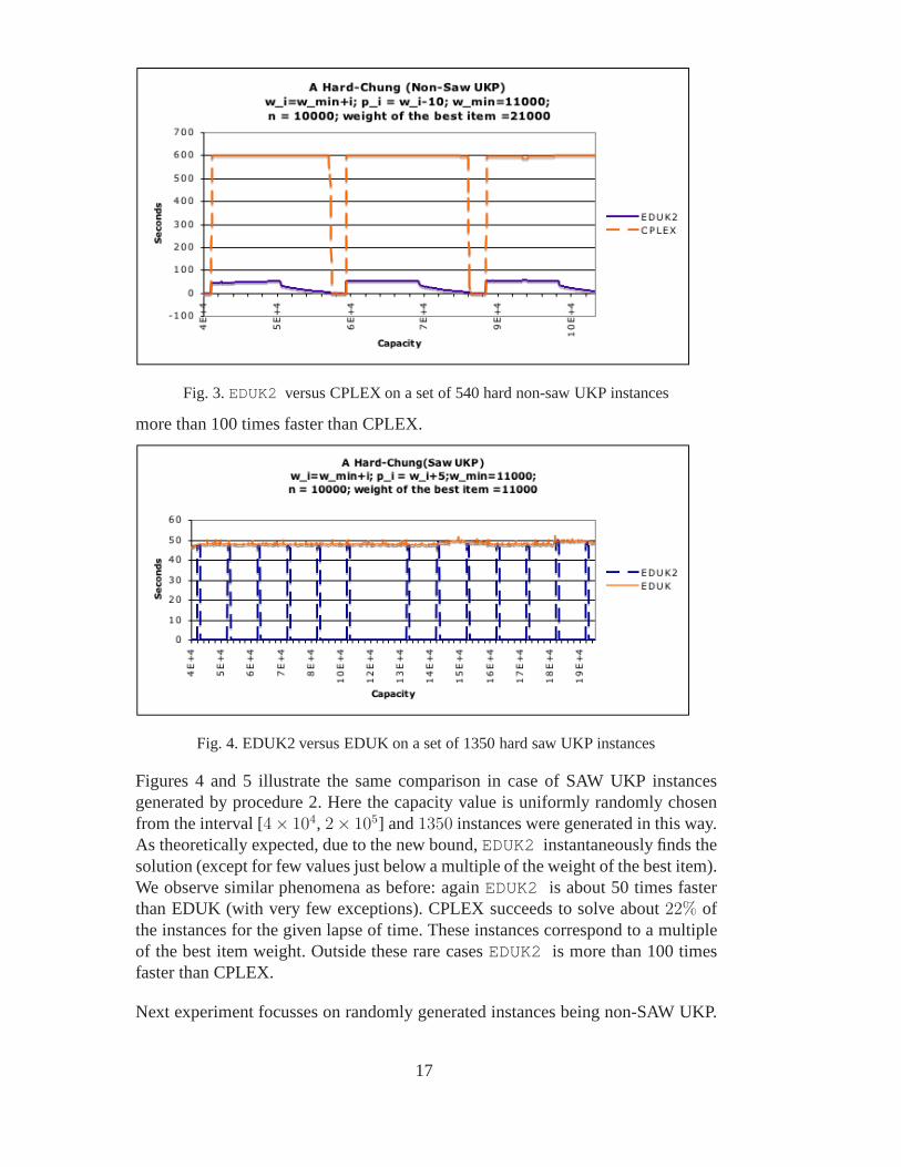
Fig. 3.EDUK2 versus CPLEX on a set of 540 hard non-saw UKP instances

more than 100 times faster than CPLEX.

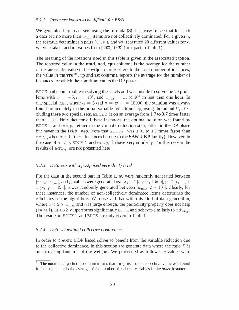
Fig. 4. EDUK2 versus EDUK on a set of 1350 hard saw UKP instances

Figures 4 and 5 illustrate the same comparison in case of SAW UKP instancesgenerated by procedure 2. Here the capacity value is uniformly randomly chosenfrom the interval [4× 104, 2× 105] and1350 instances were generated in this way.As theoretically expected, due to the new bound,EDUK2 instantaneously finds thesolution (except for few values just below a multiple of the weight of the best item).We observe similar phenomena as before: againEDUK2 is about 50 times fasterthan EDUK (with very few exceptions). CPLEX succeeds to solve about22% ofthe instances for the given lapse of time. These instances correspond to a multipleof the best item weight. Outside these rare casesEDUK2 is more than 100 timesfaster than CPLEX.

Next experiment focusses on randomly generated instances being non-SAW UKP.

17

Fig. 5. EDUK2 versus CPLEX on a set of 1350 hard saw UKP instances

We generated 2700 such instances with parameters as described in figures 7 and6 and a capacity uniformly randomly chosen from the interval[11 × 104, 43 ×104]. Fig. 6 comparesEDUK2 versus EDUK on this data set. The behavior ofboth algorithms is very similar to the one observed onFig. 2: the running time ofEDUK2 has a typical saw like shape with minima around the multiplesof the bestitem and upper-bounded by the time of EDUK.Fig. 7 illustratesEDUK2 versusCPLEX behavior. CPLEX succeeds to solve all instances with acapacity less than21 × 104 and those with a capacity close to a multiple of the best item,but failsfor all other instances with a capacity larger than21 × 104. For all these instancesEDUK2 is as at least 100 times faster than CPLEX.

Fig. 6. EDUK2 versus EDUK on a set of 2700 randomly generated UKP instances

18

Fig. 7. EDUK2 versus CPLEX on a set of 2700 randomly generatedUKP instances

5.2 Do hard UKP instances really exist?

Based on these results, one is inclined to conclude –wrongly– thatUKP are easyto solve. It is important to remind that, in the above experiments, the consideredinstances are of moderate size only. A real-life problem of the same size wouldindeed be easy to solve. However, real problems may have large coefficients, whichmakes necessary testing the solvers’ behavior on such data sets.

5.2.1 New hard UKP instances

In order to construct difficult instances, we considered data sets with large coef-ficients and/or large number of items. BecauseMTU2cannot be used for such in-stances because of arithmetic overflow, we restricted our comparisons toEDUK,eduU3

andEDUK2. For such data setsEDUK2 andeduU3benefit of thenum

ocaml library, which provides exact unlimited integer arithmetic to compute thebounds. All the runs were done on a Pentium IV Xeon , 2.8GHZ with 3GB of RAM.CPU time was limited to one hour per instance. If this time limit was reached, wereported 3600 sec. in order to compute the average9 . We use the notationxn todenotex× 10u+1 + n, where0 < ⌊ n

10u ⌋ < 10 (e.g.n = 213, 4n = 4213).

9 The notationt(k) means that the average time ist sec., withk instances reaching thetime limit.

19

5.2.2 Instances known to be difficult for B&B

We generated large data sets using the formula (8). It is easyto see that for sucha data set, no more thanwmin items are not collectively dominated. For a givenn,the formula determines n pairs(wi, pi), and we generated20 different values forc,wherec takes random values from[20n; 100n] (first part in Table 1).

The meaning of the notations used in this table is given in theassociated caption.The reported value in thenmd, ncd, cpu columns is the average for the numberof instances; the value in thewdp columns refers to the total number of instances;the value in thevrs 10 , rp andrst columns, reports the average for the number ofinstances for which the algorithm enters the DP phase.

EDUKhad some trouble in solving these sets and was unable to solvethe20 prob-lems withα = −5, n = 104, andwmin = 11 × 104 in less than one hour. Inone special case, whereα = 5 andn = wmin = 10000, the solution was alwaysfound immediately in the initial variable reduction step, using the boundUv. Ex-cluding these two special sets,EDUK2 is on an average from 1.7 to 3.7 times fasterthanEDUK. Note that for all these instances, the optimal solution wasfound byEDUK2 andedu U3

either in the variable reduction step, either in the DP phasebut never in theB&B step. Note thatEDUK2 was 1.01 to 1.7 times faster thaneduU3

whenα > 0 (these instances belong to theSAW-UKP family). However, inthe case ofα < 0, EDUK2 andedu U3

behave very similarly. For this reason theresults ofeduU3

are not presented here.

5.2.3 Data sets with a postponed periodicity level

For the data in the second part in Table 1,wi were randomly generated between[wmin;wmax], andpi values were generated usingp1 ∈ [w1;w1+500], pi ∈ [p(i−1) +1; p(i−1) + 125]. c was randomly generated between[wmax; 2 × 106]. Clearly, forthese instances, the number of non-collectively dominateditems determines theefficiency of the algorithms. We observed that with this kindof data generation,wherec < 2 × wmax andn is large enough, the periodicity property does not help(rp ≈ 1). EDUK2outperforms significantlyEDUKand behaves similarly toedu U3

.The results ofEDUK2 andEDUKare only given in Table 1.

5.2.4 Data set without collective dominance

In order to prevent a DP based solver to benefit from the variable reduction dueto the collective dominance, in this section we generate data where the ratiop

wis

an increasing function of the weights. We proceeded as follows. w values were

10 The notationx(y) in this column means that fory instances the optimal value was foundin this step andx is the average of the number of reduced variables in theother instances.

20

instance description EDUK2 eduU3EDUK

20 instances per line Hard data sets created using formula (8).c randomly from [20n; 100n].

α n wmin nmd ncd cpu vrs wdp rst rp cpu vrs wdp rst rp cpu rp

5 5 10 n n 21.77 0(13) 13 0.29 0.047 37.81 642(3) 3 0.38 0.069 80.06 0.108

15 n n 46.57 0(8) 8 0.34 0.099 52.29 83(7) 7 0.56 0.141 111.28 0.188

50 n n 154.19 0(2) 2 0.55 0.470156.63 0(2) 2 0.68 0.555 261.29 0.661

5 10 10 n n 0.03 0(20) 20 - - 135.22 2420(3) 3 0.54 0.007 336.70 0.008

50 n n 344.12 0(6) 6 0.26 0.037367.94 0(6) 6 0.41 0.052 915.11 0.079

110 n n 771.53 0(2) 2 0.20 0.112816.90 0(2) 2 0.26 0.139 2808.50 0.300

-5 5 10 n n 64.82 44(6) 6 0.78 0.091 113.67 0.108

15 n n 104.89 11(2) 2 0.61 0.091 183.31 0.188

50 n n 232.26 0(8) 8 0.86 0.650 447.40 0.660

-5 10 10 n n 167.26 1317(4) 4 0.67 0.009 317.01 0.009

50 n n 508.37 0(6) 6 0.45 0.058 1539.74 0.079

110 n n 1401.(3) 0(4) 4 - 0.124 (20) -

200 instances per line Data sets with a postponed periodicity level.c randomly from [wmax; 2 × 106]

n wmin wmax nmd ncd cpu vrs wdp rst rp cpu vrs wdp rst rp cpu rp

20 20 10n 19985 16851 118.65 11121 2 0.25 0.989 344.81 0.994

50 20 10n 50000 49999 1026.(1) 28881 0 0.22 1.00 2959.(8) 1.00

20 50 10n 19999 19924 126.(2) 9955 0 0.23 1. 504. 1

50 50 10n 50000 49999 1553.(1) 22827 0 0.32 1.00 3289.(51) 1.00

500 instances per line Data set without collective dominance (formula (9)).c randomly from [wmax..1000n]

n wmin nmd ncd cpu vrs wdp rst rp cpu vrs wdp rst rp cpu rp

5 n n n 7.93 3101 23 0.40 0.827 29.05 0.816

10 n n n 36.84 5660(1) 13 0.43 0.745 147.76 0.759

20 n n n 184.55 12010 3 0.38 0.791 735.24 0.783

50 n n n 808.26 25499 2 0.46 1 2764.59 1

SAW data sets.c randomly from [wmax; 10n]

n wmin nbi nmd ncd cpu vrs wdp rst rp cpu vrs wdp rst rp cpu rp

10 10 200 9975 1965 8.03 8015 14 0.40 0.597 11.12 5323 2 0.47 0.630 29.06 0.636

50 5 500 49925 5568 70.78 41289(1) 17 0.05 0.51108.97 25287(1) 11 0.53 0.517294.30(1) 0.521

50 10 200 49955 8983 71.02 39779(3) 6 0.40 0.49122.66 26510(3) 3 0.49 0.492 416.88 0.496

100 10 200 99809 6592 264.12 90436 1 0.32 0.510387.03 65289 1 0.45 0.519 1268.45 0.523

Table 1Data fromn and wmin columns should be multiplied by103 to get the real value. Weuse the following metrics: nmd: number of non-multiply dominated items (step 1 ofEDUK2); ncd: number of non-collectively dominated items (as computed by EDUK); cpu:running CPU time in seconds;rp : denotes the ratioy

+

c wherey+ is the capacity levelwhere the algorithm detects that the periodicity levely∗ is reached;vrs: number of itemseliminated in the variable reduction step;wdp: number of instances for which the optimalsolution was found without using DP (steps 1 to 3);rst: ratio of the number of states in theDP phase (step 4 ofEDUK2) with respect to the number of states forEDUK.

uniformly and randomly generated within the interval[wmin..wmax] (without dupli-cates) and were sorted in an increasing order. Thenp was generated using

21

p1 = pmin + k1 and

pi = ⌊wi × (0.01 +pi−1

wi−1)⌋+ ki with ki randomly generated≤ 10 (9)

We setwmin = pmin = n, wmax = 10n, andc was randomly generated within[wmax..1000n]. We did not observe any significant difference betweenEDUK2 andeduU3

, though both were about 4 times faster thanEDUK(see the associated (third)part in Table 1).

5.2.5 SAW data sets

SAW-UKP instances were generated following procedure 2 with the parameters:wmax = 1n, pmax = 2n andc ∈ [wmax; 10n]. For each pair(n, wmin), we generatednbi distinct instances(see the associated (last) part in Table 1).

The tight and computationally cheap upper bound for these sets gives a clear ad-vantage toEDUK2 compared toEDUKandedu U3

. The quality of this bound has anoticeable impact on the number of instances solved in the variables reduction stepor by the initialB&B (columnwdp), the number of reduced variables (columnvrs), and the number of states (columnrst) .

5.2.6 Summary

EDUK2consistently and significantly outperformed EDUK on all data sets. Oncemore this is illustrated onFig. 8 where the number of points plotted on the leftand the right graphics are 2500 each. Any point is an UKP instances of 20000(left) and of 50000 (right) variables. The average statistics for the running times ofEDUK2 and EDUK are: forSAW-UKP, generated according listing 2,EDUK2 is10 times faster than EDUK, while fornon-SAW-UKP - 3 times. For many in-stances,EDUK2 yielded the solution immediately while EDUK required severalminutes (sometimes more than 1 hour). The efficiency ofEDUK2 is obtained bythe cumulative effect of the different ways thatB&B and DP are integrated. Takinginto account all the new hard instances (except those generated with formula (8)),the reduction variables step reduces the number of items to be considered on anaverage varying from55% to 95%. Integrating bounds during the DP phase furtherreduces the number of states from46% to 95%. The impact of the new boundU∗

b

is important for allSAW-UKP instances and it affects all steps of the algorithm.For thenon-SAW-UKP instances no significant difference was observed betweenusingU∗

b andU3.

The superiority ofEDUK2 to the general solver CPLEX is (as expected) apparent.In the dominant case, in all tests presented in section 5.1.4EDUK2 was morethan 100 times faster than CPLEX11 . Additionally to these tests we found useful

11 CPLEX execution time was upper bounded by 600 sec.

22

Running times in seconds ofEDUK2 (on the horizontal axis) and of EDUK (on thevertical axis). Each point corresponds to one instance. Theline is the equal-timeline. Left: data set without collective dominance generated by formula (9) withn = 2 × 104. Right:SAW-UKP data set withn = 5 × 104.

Fig. 8. Plots of two large sets of instances

to check the performance ofEDUK2 in some recent UKP applications. One suchapplication is described in [16] where CPLEX has been used asUKP solver, insteadof a special purpose algorithm. We generated the same set of instances as in [16] forn = 106. EDUK2 computed 5 such instances on an average time of 0.15 seconds,while the respective running time in [16] is announced to be around 30 hours!

There are still hard instances with large values forn andwmin, notably those gener-ated with formula (8), whereα < 0, wmin = 110000, n = 10000. They were solvedby EDUK2 on an average of25 to 30 minutes. For all these difficult instances, thenumber of items that are not collectively dominated is very large. Thus, it appearsthat for such cases, DP algorithm needs to explore a huge iteration space whenB&B fails to discover the solution.

6 Conclusion

We have shown that a hybrid approach combining several knowntechniques forsolving UKP performs significantly better than any one of these techniques usedseparately. The effectiveness of the approach is demonstrated on a rich set of in-stances with very large inputs. The combined algorithm inherits the best timingcharacteristics of the parents (DP with bounds andB&B). We also proposed a newupper bound for the UKP and demonstrated that this bound is the tightest oneknown for a specific family of UKP. OurEDUK2 algorithm takes advantages ofmost of the known UKP properties and is able to solve all but the very special hardproblems in a very short time. It appears that instances, previously known to bedifficult, are now solvable in less than a few minutes.

Acknowledgements Supported by Hubert Curien French-Bulgarian partnershipRILA 2006 N0 15071XF. All computations were done on the Ouest-genopole bioin-formatics platform (http://genouest.org). Thanks to N. Malod-Dognin for his helpin running CPLEX. The authors would like to thank the two anonymous referees fortheir insightful comments, corrections and suggestions that significantly improvedthe paper.

23

References

[1] R. Andonov, V. Poirriez, and S. Rajopadhye. Unbounded knapsack problem : dynamicprogramming revisited.European Journal of Operational Research, 123(2):168–181,2000.

[2] D. Babayev, F. Glover, and J. Ryan. A new knapsack solution approach byinteger equivalent aggregation and consistency determination. INFORMS Journal onComputing, 9(1):43–50, 1997.

[3] V. Boyer, M. Elkihel, and D. El Baz. Efficient heuristics for the 0/1 multidimensionalknapsack. InROADEF, pages 95–106. Presses Universitaires de Valenciennes, 2006.

[4] L. Caccetta and A. Kulanoot. Computational Aspects of Hard Knapsack Problems.Nonlinear Analysis, 47:5547–5558, 2001.

[5] C-S. Chung, M. S. Hung, and W. O. Rom. A Hard Knapsack Problem.Naval ResearchLogistics, 35:85–98, 1988.

[6] R. Garfinkel and G. Nemhauser.Integer Programming. John Wiley and Sons, 1972.

[7] P. C. Gilmore and R. E. Gomory. The Theory and Computationof KnapsackFunctions.Operations Research, 14:1045–1074, 1966.

[8] S. Martello, D. Pisinger, and P. Toth. Dynamic programming and strong bounds forthe 0-1 knapsack problem.Manag. Sci., 45:414–424, 1999.

[9] S. Martello and P. Toth. A mixture of dynamic programmingand branch-and-boundfor the subset-sum problem.Manag. Sci., 30(6):765–771, 1984.

[10] S. Martello and P. Toth. Knapsack Problems: Algorithms and ComputerImplementations. John Wiley and Sons, 1990.

[11] G. L. Nemhauser and L.A. Wolsey.Integer and Combinatorial Optimization. JohnWilley & Sons, 1988.

[12] U. Pferschy, H. Kellerer, and D. Pisinger.Knapsack Problems. Springer, 2004.

[13] G. Plateau and M. Elkihel. A hybrid algorithm for the 0-1knapsack problem.Methodsof Oper. Res., 49:277–293, 1985.

[14] V. Poirriez and R. Andonov. Unbounded Knapsack Problem: New Results. InWorkshop Algorithms and Experiments (ALEX98), pages 103–111, February 1998.

[15] V. Poirriez, N. Yanev, and R. Andonov. Towards reduction of the class of intractableunbounded knapsack problem. Research report, LAMIH/ROI UMR CNRS-UVHC8530, 2004.

[16] C. Srisuwannapa and P. Charnsethikul. An exact algorithm for the unboundedknapsack problem with minimizing maximum processing time.Journal of ComputerScience, 3(3):138–143, 2007.

[17] Nan Zhu and Kevin Broughan. On dominated terms in the general knapsack problem.Operations Research Letters, 21:31–37, 1997.

24