A House Without a Ring · to be homeowners. 1California rst enacted the no-fault divorce in 1969....
64
A House Without a Ring: The Role of Changing Marital Transitions for Housing Decisions Minsu Chang * November 13, 2018 Latest Version Available Here Abstract This paper shows that the evolving likelihood of marriage and divorce is an essential factor in accounting for the changes in housing decisions over time in the United States. To quantify the importance of this channel, I build a life-cycle model of single and married households who face exogenous age-dependent marital transition shocks. I then estimate the parameters of the model by a limited information Bayesian method to match the moments from 1995’s cross-section data. I conduct a decomposition analysis between 1970 and 1995, two years with similar real house prices but substantially different probabilities of marital transitions. I find that the change in the likelihood of marital transitions accounts for 29% of the observed increase in the homeownership rate of singles. This portion is substantial given that the changes in downpayment requirements, earnings risk, and spousal labor productivity jointly replicate 45% of the change. When the change in marital transitions is shut down, the marrieds’ housing asset share increases, which is opposite to the data’s pattern. Then I extend my analysis to study whether the ongoing change in marital transitions still plays a role in explaining housing decisions in recent years, which have seen dramatically changing house prices. In addition to other factors such as credit constraints, wages, and beliefs on price appreciation that are often suggested as drivers for homeownership increase during the housing boom in the mid-2000s, I show that the continuing decrease in marriage contributes to an approximately 7% increase in the homeownership rate for young singles. Keywords: Homeownership; Portfolio Share; Marriage; Divorce; Household Formation; House Prices; * Department of Economics, University of Pennsylvania, 133 South 36th Street, Philadelphia, PA 19104. Email: [email protected]. I would like to thank my advisors, Jes´ us Fern´ andez-Villaverde and Frank Schorfheide, for their guidance and support throughout this project. I have also benefited from helpful comments by Harold Cole, Frank DiTraglia, Dirk Kr¨ uger, Andrew Postlewaite, Jos´ e-V´ ıctor R´ ıos-Rull, and participants at the UPenn Macro Seminar, UPenn Econometrics Seminar, and the MFM Summer Session for Young Scholars. All remaining errors are my own.
Transcript of A House Without a Ring · to be homeowners. 1California rst enacted the no-fault divorce in 1969....

A House Without a Ring:
The Role of Changing Marital Transitions
for Housing Decisions
Minsu Chang∗
November 13, 2018
Latest Version Available Here
Abstract
This paper shows that the evolving likelihood of marriage and divorce is an essential factorin accounting for the changes in housing decisions over time in the United States. To quantifythe importance of this channel, I build a life-cycle model of single and married householdswho face exogenous age-dependent marital transition shocks. I then estimate the parametersof the model by a limited information Bayesian method to match the moments from 1995’scross-section data. I conduct a decomposition analysis between 1970 and 1995, two yearswith similar real house prices but substantially different probabilities of marital transitions. Ifind that the change in the likelihood of marital transitions accounts for 29% of the observedincrease in the homeownership rate of singles. This portion is substantial given that the changesin downpayment requirements, earnings risk, and spousal labor productivity jointly replicate45% of the change. When the change in marital transitions is shut down, the marrieds’ housingasset share increases, which is opposite to the data’s pattern. Then I extend my analysis tostudy whether the ongoing change in marital transitions still plays a role in explaining housingdecisions in recent years, which have seen dramatically changing house prices. In addition toother factors such as credit constraints, wages, and beliefs on price appreciation that are oftensuggested as drivers for homeownership increase during the housing boom in the mid-2000s, Ishow that the continuing decrease in marriage contributes to an approximately 7% increase inthe homeownership rate for young singles.
Keywords: Homeownership; Portfolio Share; Marriage; Divorce; Household Formation; House Prices;
∗ Department of Economics, University of Pennsylvania, 133 South 36th Street, Philadelphia, PA 19104.Email: [email protected]. I would like to thank my advisors, Jesus Fernandez-Villaverde and FrankSchorfheide, for their guidance and support throughout this project. I have also benefited from helpfulcomments by Harold Cole, Frank DiTraglia, Dirk Kruger, Andrew Postlewaite, Jose-Vıctor Rıos-Rull, andparticipants at the UPenn Macro Seminar, UPenn Econometrics Seminar, and the MFM Summer Sessionfor Young Scholars. All remaining errors are my own.

1
1 Introduction
Owner-occupied housing represents the largest asset of most households’ net worth. Fur-
thermore, it is often argued that owner-occupied housing is associated with desirable policy
goals such as better-maintained neighborhoods and better educational outcomes for the chil-
dren living in them. Thus, it is not a surprise that many countries have encouraged home
purchase by policies such as mortgage subsidies and tax benefits. This means that, to as-
sess the effectiveness of such policies, it is crucial to study which factors affect households’
housing decisions. This paper argues that the evolving likelihood of marriage and divorce is
an essential factor in accounting for the change in homeownership rate and composition of
household net worth over time.
Figure 1 shows the likelihood of marital transitions, homeownership rate, and housing
asset share — net housing value divided by the total asset — in 1970 and in 1995. I pick
1970 as a representative period of high marriage and low divorce risks for two reasons: first,
it is not easy to get information on households’ portfolios with data prior to 1970; second,
a number of changes happened after 1970 in social norms associated with marriage and
divorce. One leading example is the legalization of no-fault divorce over the 1970s, in which
the dissolution of marriage does not require proof of wrongdoing by either spouse.1 As a
period of low marriage and high divorce risks, I choose 1995 because real house prices were
similar in levels but the probabilities of marital transitions differed substantially between
1970 and 1995. Once the analysis between 1970 and 1995 is done, changing house prices will
be incorporated to study recent years after 1995.
The top-left panel in Figure 1 shows marriage probabilities conditional on the age of
household head. Young singles in 1995 were much less likely to get married compared to
those in 1970. In the top-right panel, the singles’ homeownership rate displays a significant
increase from 1970 to 1995. I argue that this change in the homeownership rate can be
accounted for at least partially by the change in the likelihood of marriage. If a single is
likely to get married soon, he/she will wait to buy a house with a spouse because transaction
costs make it costly to sell or resize a house. Furthermore, the prospect of marriage creates
a free rider problem that discourages singles from saving, which makes it less likely for them
to be homeowners.
1California first enacted the no-fault divorce in 1969. By late 1983, all the states except for South Dakotaand New York had legally allowed no-fault divorce. It is still controversial whether this law raised divorcerates (Friedberg, 1998; Wolfers, 2006). Instead of taking a stand on causal effect, I interpret the legalizationof no-fault divorce as a signal of change in social norms about marriage and divorce.

2
Marriage Probabilities Homeownership of the Single
Divorce Probabilities Housing Asset Share of the Married
Figure 1: Likelihood of Marital Transitions and Housing Decisions (1970 vs. 1995)
Note: Section 2 and Section 4 of this paper include details on how these figures are generated.
Divorce rates increased sharply over the 1970s as a marriage was no longer regarded as
mandatory. The bottom-left panel of Figure 1 shows that divorce probabilities increased
across all age groups from 1970 to 1995. The bottom-right panel shows the housing share in
total assets of married households. Compared to those in 1970, young married households in
1995 held a lower fraction of total assets in housing. I show that this pattern can be generated
by the change in the likelihood of marital transitions. A married couple will invest less in
housing if the partners are more likely to get divorced, because it is more difficult to split a
house than liquid assets such as checking accounts.
In summary, I hypothesize that the change in housing decisions is affected by the change
in the likelihood of marital transitions in a quantitatively important way. Similar to Cubeddu

3
and Rıos-Rull (2003) and Fernandez and Wong (2014), I study this hypothesis by taking
marriage and divorce as exogenous shocks households face. This is in a similar vein to the
previous literature treating employment status or earnings as exogenous shocks that shape
households’ decisions. Then I vary the underlying probabilities over time to reflect the
observed changes in household formation from the data.
To quantify the effect of the change in marital transitions on the change in homeownership
and housing asset share, I build a life-cycle model of single and married households that face
age-dependent marital transition shocks. In other words, households consider the prospect of
marriage and divorce when making decisions. They decide how much to consume, rent, save
in non-housing and housing assets, and work. Owned housing incurs substantial transaction
cost whenever its size is adjusted. Especially in times of getting married or divorced, this
cost is modeled to arise because a status change makes the house owned prior to the change
no longer suitable. This is empirically supported by the fact that, although some couples
move in to the home that one partner already has, they tend to sell the house and move to
another one within 5 years of marriage, which is the unit of my model period (Speare and
Goldscheider, 1987). Likewise, divorcees are likely to move to a new house since the house
bought as a married couple would not meet their needs after divorce (South et al., 1998).
In addition, I model the following features to reflect other changes that may have affected
housing decisions: (i) A finite number of housing sizes are available to own, each of which
can serve as a collateral for borrowing. This is useful to isolate the role of relaxed borrowing
constraints on lumpy housing decisions. (ii) Households face idiosyncratic labor productivity
shocks. This enables me to analyze how households adapt their housing investment to
increasing earnings risk. (iii) Each household member decides how much to work. As a
spouse’s labor productivity increases, the model generates the increase in spousal labor
supply while allowing for a household head to adjust his/her labor supply accordingly.
I structurally estimate the parameters of the model by a limited information Bayesian
method to match the moments from the cross-section data of 1995, the benchmark year for
my analysis. The model closely fits the life-cycle profiles of homeownership, housing asset
share, and labor force participation across marital status observed in the data. The estimated
parameters inform us about the substitutability of renting and owning a house, utility from
home production, economies of scale within marriage, and cost associated with labor supply.
Then, I conduct a decomposition analysis to quantify how much of the change in housing
decisions between 1970 and 1995 can be accounted for by the change in the likelihood of

4
marital transitions. These two years are treated as steady states with the same housing
prices, but very different marriage and divorce prospects.
First, I find that the change in the likelihood of marital transitions accounts for 29%
of the observed change in singles’ average homeownership rate. This channel is useful to
generate a homeownership rate of singles aged 25 to 30 that is much lower in 1970 compared
to 1995. I also incorporate other changes in key drivers of housing decisions studied in
the literature: borrowing constraints, earnings risk, and spousal labor productivity. When
combined, these channels account for 45% of the observed change. The comparison with the
marital transition channel, which accounts for 29% of the observed change, demonstrates
that the change in marital transitions is quantitatively of comparable importance to the
changes in borrowing constraints, earnings risk, and spousal productivity.
Second, in the data, the average share of assets held in housing by married households
declined by 11% between 1970 and 1995. The model can only reproduce this decline if
the changes in marital transitions are included. In their absence, the other drivers predict
an increase in this share, again demonstrating the crucial importance of this channel for
observed trends in households’ housing decisions. In addition to getting the consistent sign
of change as observed in the data, all the combined channels generate 31% of the observed
change in housing asset share of the married.
It is then an obvious question whether marital transitions, which have continued to
change, still play a role in explaining the evolution of housing variables in recent years when
house prices have changed dramatically. To incorporate the changing house prices, I model
the common house price as a stochastic shock similar to Corbae and Quintin (2015), thereby
replicating the house price boom-bust episode in the 2000s. I also include a belief shock
on appreciation to generate the surge in homeownership during the boom. I simulate the
homeownership rate with changing house prices, beliefs on appreciation, credit constraints,
and wages. These changes are set to mimic the recent experiences in the housing market.
The reduction in marriage and divorce probabilities observed in the data increases the
singles’ homeownership rate by 6.8% whereas it decreases the marrieds’ homeownership
rate by 3.2% during the boom. The changes in credit constraints, wages, and beliefs on
appreciation were often suggested as drivers for homeownership increase during the boom,
which is also supported by my paper. It is worth noting that the change in marital transitions
contributes to replicate the homeownership increase for young singles even when the house

5
price was expensive. In contrast, the change in marital transitions puts downward pressure
on the marrieds’ homeownership, which is masked by the other factors during the boom.
This paper contributes to several distinct strands of literature. First, it is related to
the literature on household portfolio choice with housing. An important stream of papers
analyzes the implication of housing as illiquid asset in theoretical models of portfoilo choice
(Grossman and Laroque, 1990; Flavin and Yamashita, 2002; Stokey, 2009). Most quan-
titative papers on portfolio choice with housing rely on a life-cycle framework, motivated
from empirically conspicuous life-cycle patterns in housing decisions (Cocco, 2005; Yao and
Zhang, 2005; Fernandez-Villaverde and Krueger, 2007; Kaplan and Violante, 2014). My
paper builds on these while modeling transaction cost that arises in times of marital transi-
tions. This captures the friction from the idiosyncratic nature of housing investment in that
a status change would make the house owned prior to the change unsuitable.
Second, this paper demonstrates the importance of change in idiosyncratic risk on aggre-
gate variables, which is also emphasized in the literature. For instance, idiosyncratic income
shocks are analyzed to affect various aggregate variables such as income and consumption
inequality (Blundell et al., 2008; Heathcote et al., 2010), output and associated welfare (Low
et al., 2010), and homeownership (Diaz and Luengo-Prado, 2008). My paper studies the
aggregate implication of idiosyncratic shocks, including marital transition risk and earnings
risk, on homeownership and households’ portfolios over time. Furthermore, I study how
the change in marriage and divorce probabilities affects these housing variables differently
between singles and married households.
Third, this paper contributes to the literature that analyzes the importance of marital
transitions for households’ decisions. This includes various non-housing decisions such as
savings and female labor supply (Cubeddu and Rıos-Rull, 2003; Mazzocco et al., 2007;
Fernandez and Wong, 2014; Voena, 2015), fertility and child investment (Brown and Flinn,
2011), and portfoilo choice without housing (Love, 2010). Few recent papers attempt to
study housing decisions in the presence of marital transitions. Fisher and Gervais (2011),
for example, generate the decrease in the aggregate homeownership of the young by a trend
of marrying later and having more singles in the economy. However, as opposed to my
model, their framework cannot replicate the increase in young singles’ homeownership rate
observed in the data. Fischer and Khorunzhina (2016) study the role of divorce risk on
housing decisions by comparing the simulated life-cycle profiles for those with and without
divorce risk. I attempt to link my model to the historical data to quantify how much of
the change in the likelihood of marriage and divorce can account for the change in housing

6
decisions. To the best of my knowledge, my paper is the first study to quantify this effect
with estimation using the micro data.
The rest of the paper is organized as follows. Section 2 describes the data and establishes
the empirical facts. Section 3 outlines the model, and Section 4 explains how to calibrate
and estimate the parameters and provides the model fit. Section 5 shows the decomposition
analysis, which quantifies how much of the change in housing decisions can be accounted
for by the change in the likelihood of marital transitions between 1970 and 1995. Section 6
extends the framework to incorporate the changing house prices to study the recent periods.
Section 7 concludes.
2 Data
In this section, I illustrate the data sources used to construct the life-cycle profiles of
housing variables in 1970 and 1995. It is worth noting that the real house price was quite
stable between the two years.2 To control for this confounding factor, I chose 1970 and 1995
because the house prices were similar in level, but the likelihood of marital transitions differed
substantially. The year 1970 was chosen as a representative period with high marriage and
low divorce probabilities. If we look at the time series data3, the marriage rate showed a
local peak in 1970 and started to fall from then on. In contrast, with the legalization of
no-fault divorce, the divorce rate surged throughout the 1970s.4 The year 1995 was chosen
as the benchmark period with high divorce and low marriage probabilities. It is suitable for
the analysis in that it is after the housing recession in 1990 and before the start of housing
price boom in late 1990s, a trend that continued until the Great Recession.
I cover different time periods in the separate sections. In Section 5, I conduct a decompo-
sition analysis between 1970 and 1995 to study how much of the change in marital transition
probabilities can explain the change in housing decisions, controlling for the house price.
However, the house price increased dramatically over the early 2000s. In addition, the mar-
ital transition probabilities continued to change, although the magnitude of change became
small. In Section 6, I extend my analysis and study the implication of marital transition
probabilities on housing decisions under changing house prices.
2See Corbae and Quintin (2015) for the time series of the real house price index. The price to rent ratioalso shows a similar trend as reported in Gallin (2008).
3Source: Centers for Disease Control and Prevention National Center for Health Statistics (CDC NCHS)4See Voena (2015) for the overview of U.S. divorce laws and for the literature review.

7
2.1 Data to construct life-cycle profiles in 1995
I use the 1995 Survey of Consumer Finances (SCF), which is conducted every three
years and is available from the Federal Reserve’s website. This data is a repeated cross-
section that provides detailed information on the households’ portfolio choices as well as
their demographic characteristics such as age and marital status.
To be consistent with my model, I categorize assets into either housing or non-housing
assets.5 The SCF also provides information on mortgages and home equity lines of credit,
which can be used to construct the net value of housing assets. Then I construct the variable
housing asset share as the net value of housing assets divided by the total assets, including
both housing and non-housing assets. I focus on the unconditional share, which combines
the information about participation rate and conditional housing asset share. The life-cycle
profile of this unconditional share still preserves a hump shape. The variable homeownership
is defined as a dummy variable whose value is one if a household holds a positive amount of
housing assets. Regarding a household’s labor supply, I use the employment status and the
weekly hours of work reported in the SCF data.
To analyze the more recent years, I use the SCF data for 2007, 2010, and 2013. The year
2007 represents the housing boom period. The years 2010 and 2013 together give information
about the recovery period after the bust. The way the variables are constructed is analogous
to that of 1995, and hence it is omitted.
2.2 Data to construct life-cycle profiles in 1970
I use two data sources to construct life-cycle profiles for the year 1970. First, I use
the 1970 Survey of Consumer Finances. This data is accessible via the Inter-University
Consortium for Political and Social Research (ICPSR), whereas the SCF data since 1983 is
available from the Federal Reserve’s website. I use the raw data downloaded from ICPSR
and construct the variables of interest as outlined in Appendix A. The value of using the
historical SCF data before 1983 has recently been highlighted by Kuhn et al. (2017), and my
paper is also in line with their attempt to incorporate this data to answer a question that
has not been answered: How much of the change in homeownership and housing asset share
can be accounted for by the change in marital transition probabilities?
5The description on how each variable is constructed is provided in Appendix A.

8
However, there is a challenge to answering this question because the number of observa-
tions of single households in the 1970 SCF is too small due to the high marriage rate. This
results in a very jagged life-cycle profile for single households. To obtain more observations
that can inform us about homeownership rate and housing asset share in 1970, I use the
Panel Study of Income Dynamics (PSID) data, which is the longitudinal household survey
that has been administered since 1968.
Despite the larger number of observations in the 1970 PSID, it does not provide enough
information on households’ non-housing asset composition, which is essential information
to construct the housing asset share variable. Therefore, I use a cross-imputation strategy
similar to Blundell et al. (2005) to obtain a relation between housing assets and non-housing
assets from the 1970 SCF data and impute the missing non-housing assets for the PSID
sample using the fitted regression. The cross-imputation is done as follows: using the 1970
SCF sample, I first add 1% of average net value of housing to each household i’s net value
of housing, denoted by net value of housing†i,SCF . This is done in order to secure more
observations used in the regression of log-log specification. I regress this logged net value of
housing on the logged non-housing asset with various controls included in Xi,
log(net value of housing†i,SCF ) = X ′i,SCFβ + γ log(non-housing asseti,SCF ) + ui,SCF .
By using the estimated coefficients (β, γ) and assuming that the relation between vari-
ables will be the same between the different data sets, we can obtain the cross-imputed value
of non-housing assets in the PSID data for household i as
non-housing asseti,PSID = exp
(log(net value of housing†i,PSID)−X ′i,PSIDβ
γ
).
Using the imputed non-housing asset value and the observed housing asset value, I con-
struct the housing asset share for household i in the PSID as
housing asset sharei,PSID =net value of housingi,PSID
net value of housingi,PSID + non-housing asseti,PSID.
In Table 11 in Appendix A, I show that the regression applied to the 1970 SCF data to
obtain the estimates (β,γ) has an adjusted R-squared close to 0.8. Also, I show that the
mean, the median, and the standard deviation of the imputed housing asset share of the
PSID data are close to those observed in the SCF data.

9
2.3 Life-cycle profiles in 1970 and 1995
I construct the life-cycle profiles of single and married households in 1970 and 1995. Fig-
ure 2 shows the change in homeownership rate and housing asset share over time depending
on marital status. First, the singles’ homeownership rate increased significantly across all
age groups between the two years. This is also the case for the singles’ housing asset share.
Since the pattern of change is qualitatively similar for the two housing variables, I focus on
the change in homeownership in the following sections.
Homeownership of the Single Homeownership of the Married
Housing Asset Share of the Single Housing Asset Share of the Married
Figure 2: Homeownership Rate and Housing Asset Share
Note: All figures show the average homeownership rate and the average housing asset share acrossdifferent age groups. The x-axis stands for the age of household head. Housing asset share isdefined to be the net housing value divided by the total assets.

10
For the married, the homeownership rate did not change significantly between 1970 and
1995 for younger households from age 25 to age 44.6 In contrast, the homeownership rate
increased significantly for older married households. Given that the main channel of interest
— the change in the likelihood of marriage and divorce — matters mostly for the young, it
is not expected to explain the increase in the homeownership rate for older people. What
explains this change is left for future research. Interestingly, the housing asset share was
higher in 1970 compared to 1995 for younger married households.7 I focus on this change in
portfolio share of young married couples instead of the change in homeownership rate. This
is why Figure 1 includes the two housing variables showing significant changes.
Many papers have attempted to explain the pattern that married households are more
likely to be homeowners than singles. In addition to this observation from the cross-section, I
aim to account for the within-group change in housing variables over time; first, the increase
in the singles’ homeownership rate, and second, the decrease in the marrieds’ housing asset
share. I highlight that it is important to focus on heterogeneity in terms of marital status in
understanding the over-time changes in housing decisions. Then I argue that the likelihood
of household formation and dissolution plays a major role in generating these changes over
time. If a single is likely to marry soon, he will wait to buy a house with a spouse because
it is costly to sell or re-size a house. Furthermore, the prospect of marriage creates a free
rider problem that discourages singles from saving, which makes it less likely for them to be
homeowners. This may explain why the singles’ homeownership rate increased as they were
less likely to marry. In addition, a married couple who are likely to get divorced will tilt their
portfolio away from housing asset since it requires a large transaction cost when liquidation
happens with a divorce. To formalize this conjecture and quantify how much of the change
in marital transition probabilities can account for the change in housing variables, we need
a structural model.
3 Life-cycle model
I develop a life-cycle model of single and married households who face age-dependent
marital transition shocks. Similar to Cubeddu and Rıos-Rull (2003) and Fernandez and
6The null hypotheses of equal means are not rejected under 5% significance level for the age groups25-29, 30-34, 35-39, and 40-44.
7The null hypotheses of equal means are rejected under 5% significance level for age 25-30 and 35-40 andrejected under 10% significance level for age 30-35 (p-value = 0.07).

11
Wong (2014), marital status is treated as exogenous in order to build a computationally
tractable model of heterogeneous households.8 When making decisions, households will take
into account the probability of getting married or divorced.
Households decide how much to consume, rent, save in non-housing and housing assets,
and how many hours to work. For housing decisions, a finite number of housing sizes are
available to own. Owning a house is advantageous since it yields a higher service flow than
renting and it serves as a collateral for borrowing. However, it incurs substantial transaction
cost whenever its size is adjusted. Housing is a highly idiosyncratic investment, so a change
in status would make the house owned prior to the change no longer suitable. For example,
when you are single, you do not know what type of house your future spouse may like. When
you get married, you learn how your spouse values the jointly owned home. The house you
purchased as single is likely to be ill-suited for a married couple. Hence, it is modeled that
the owned house is sold and the associated transaction cost arises in times of getting married
or divorced.
Households face non-insurable idiosyncratic labor productivity shocks and idiosyncratic
housing price shocks. The framework is a partial equilibrium model in which households
face the following exogenous prices: wage, savings interest rate, borrowing interest rate, and
common house price. For now, the common house price is set to be fixed to analyze the
steady states. In Section 6, the common house price will be modeled as a stochastic shock
to study more recent periods with changing house prices.
Preference - Single agent. A single agent’s utility is specified by
u(c, s, l) =(cαs1−α)(1−σ)
1− σ−Bs
l1+ 1γ
1 + 1γ
− φ · I(l > 0) + uhp(l),
where c ≥ 0 is consumption and s ≥ 0 is housing service. The service is defined as s =
m + ζ(h) · h, where m is from rented housing and ζ(h) · h is from owned housing. ζ(h) is a
size-dependent function of owned housing
8Although people choose which type of family arrangement they live in, this paper treats it as exogenousshocks stochastically generated by underlying probability distribution. On the other hand, there are a fewrecent papers that endogenize households’ marital decisions in different contexts. For example, see Low etal. (2018) and Reynoso (2018).

12
ζ(h) =
(ζ1 + ζ2
h− hminhmax − hmin
),
where hmin is the smallest non-zero size of owned housing and hmax is the biggest size. ζ1 is
the service gain of owning hmin-sized housing compared to renting. ζ2 reflects the marginal
gain for larger houses. ζ(h) is assumed to be greater than 1 to reflect that owned housing is
preferred to rented housing.9
On top of the change in marital transitions, there were substantial changes in earnings
risk and in the labor market environment between 1970 and 1995. Since I want to incorporate
these changes to the decomposition analysis in Section 5, I build a model with endogenous
labor supply. This will allow us to study how housing decisions as lumpy investments change
according to how agents adjust their hours in response to various idiosyncratic shocks. l
stands for labor supply associated with disutility from working Bs and fixed cost of labor
market participation φ. Also, there is utility from home production
uhp(l) =
0 if one works
ωuhp if one does not work.
The utility from home production while working is normalized to be zero. The parameter
ωuhp is identified from φ since I adopt a different functional form for the married agent’s utility
from home production.
Preference - Married agents. Within a married household, there is a head and a spouse.
They differ in terms of labor productivity denoted by y for the head and y for the spouse.
This can be interpreted as each member of the household taking on a role depending on
comparative advantage in house management.
A married head’s utility uhead and a married spouse’s utility uspouse are specified below:
uhead(c, s, l, l) = ϕj
((γec)
α(γes)1−α)1−σ
1− σ−Bm
l1+ 1γ
1 + 1γ
− φ · I(l > 0) + uhp(l, l)
9One could modify the owned house more easily to cater one’s needs. Also, there could be a moral hazardissue with leasing agents, which makes renting less favorable, as pointed out in Postlewaite et al. (2008).

13
uspouse(c, s, l, l) = ϕj
((γec)
α(γes)1−α)1−σ
1− σ− Bm
l1+ 1γ
1 + 1γ
− φ · I(l > 0) + uhp(l, l),
where c, s ≥ 0 is joint consumption and joint housing service. γe is a parameter that
transforms joint objects into per capita terms. If γe is greater than 0.5, it captures economies
of scale in consumption and service flow provided by marriage. ϕj allows for the marginal
utility of consumption and housing service to differ over the life-cycle. ϕj > 1 could result
from the joy of having a partner or children. Both the head and the spouse are constrained
to enjoy equal consumption and housing service.
l is labor supply of the head and l is labor supply of the spouse. Labor supply is associated
with disutility from working Bm, Bm and fixed cost of working φ, φ. The married agent’s
utility from home production is defined as
uhp(l, l) =
0 if both work
ωuhpnψ
if only one spouse works
ωuhp if no one works,
where nψ reflects whether home production technology is increasing returns to scale or not.
In an extreme case where nψ = 1.0, having two people stay at home and do the housework
generates the same utility as having one person do so.
3.1 Problem of the single at the terminal age
This section describes the recursive formulation of the single’s problem at the terminal
age J . The value function depends on the following state variables: age J , total asset a,
housing asset h, and labor productivity y. Households face exogenously given wage w, risk-
free savings interest rate r, borrowing interest rate rH , and common housing price PH . To
simplify the notation, I denote the vector of all the state variables as XsJ = [J, a, h, y].

14
V s(XsJ) = max
c,m,b′,h′,lu(c, s, l) + βV s,fin(b′, h′)
s.t. c+m+ b′ + PHh′ = wyl + a− Φ(h′, h)
c ≥ 0, s ≥ 0, b′ ≥ 0.
Φ(h′, h) is the asymmetric transaction cost associated with illiquid housing asset. Similar
to Yang (2009), it is defined as
Φ(h′, h) =
κbPHh′ + κsPHh if h′ 6= h
0 if h′ = h,
where κb < κs. Households are borrowing-constrained at the terminal age, which is captured
by non-housing asset b′ being non-negative.
The objective is to maximize the combination of current period utility and the discounted
continuation value of the remaining life. V s,fin(b′, h′) is the continuation value after age J , for
4 more periods where the household consumes the constant amount of A ≡ (b′+PHh′) 1−β1−β4 .
The amount A is obtained by assuming that the discount factor during the retirement is
equal to 1(1+r)
. This can be considered as submitting (b′ + PHh′) and entering a retirement
community, which provides in return a constant flow of utility in the future. The continuation
value in this case is written as
V s,fin(b′, h′) =1− β4
1− β· A
(1−σ)
1− σ.
3.2 Problem of the married at the terminal age
A married household’s problem at age J depends on one more state variable compared
to their single counterparts, since we also need to consider the labor efficiency shock y of a
spouse. Similarly, I denote the vector of all the state variables as XmJ = [J, a, h, y, y].

15
A married household solves a joint problem that maximizes the average utility with equal
weights. In other words, a marriage is a contract to obey the decision of a utilitarian social
planner maximizing the average utility. The average utility at the current period is
u(c, s, l, l) =uhead(c, s, l, l) + uspouse(c, s, l, l)
2
= ϕj
((γec)
α(γes)1−α)1−σ
1− σ− 1
2
(Bm
l1+ 1γ
1 + 1γ
+ Bml1+ 1
γ
1 + 1γ
)− 1
2
(φ · I(l > 0) + φ · I(l > 0)
)+ uhp(l, l).
Then the problem solved by the married household is
V m(XmJ ) = max
c,m,b′,h′,l,lu(c, s, l, l) + βV m,fin(b′, h′)
s.t. c+m+ b′ + PHh′ = w(yl + yl) + a− Φ(h′, h)
c ≥ 0, s ≥ 0, b′ ≥ 0.
The household’s labor income includes both the head’s and the spouse’s labor income.
The choice variables are analogous to the single household’s problem except that the married
household also needs to decide labor supply of the spouse l.10
The continuation value V m,fin(b′, h′) is analogous to the single’s case. The household does
not face marital transition shock at the terminal age J . Each member of the household is
assumed to identically evaluate the joint consumption amount A = (b′+PHh′) 1−β1−β4 provided
by the retirement community. There is efficiency gain γe in consumption from marriage.
The continuation value then becomes
V m,fin(b′, h′) =1− β4
1− β· ϕJ
(γeA)(1−σ)
1− σ.
10Marriage in this setup is interpretable as the change in one’s preference to care about the other membersin the household. Instead of the arrangement set by a utilitarian social planner, the married household’sproblem can also be understood as each spouse having the identical non-egoistic preference u(c, s, l, l) asabove. Then the agent’s problem, given the joint budget constraint, amounts to the problem solved by themarried household.

16
3.3 Problem of the single at the non-terminal age
At the non-terminal age, the expected value should take into account the marital shock. I
denote the vector of all the state variables as Xsj = [j, a, h, y]. The single household’s problem
at age j < J is written as follows:
V s(Xsj ) = max
c,m,b′,h′,l
u(c, s, l
)+ β
[qss,j · EV s
(j + 1, a′, h′, y′
)
+ qsm,j · EV m(j + 1, (a′ + a′)− κsPH(h′ + h′), 0, y′, y′
)]
s.t. c+m+ b′ + PHh′ = wyl + a− Φ(h′, h)
a′ = (1 + r(b′))b′ + PH(1− δ′)h′, where r(b′) =
r if b′ ≥ 0
rH otherwise
c ≥ 0, s ≥ 0, b′ ≥ −ηPHh′ with 0 ≤ η ≤ 1.
The single household’s value function depends on the same state variables as in the
terminal period’s problem. A single stays single with age-dependent probability qss,j. Then
the expected value is based on the current period savings and housing choice in addition
to future labor efficiency. The single household gets married with probability qsm,j. This
renders the continuation value equal to the average utility from the marriage arrangement.
It is assumed that one gets married to a spouse of the same age group. This is consistent
with the empirical fact that the average age differential of a married couple is 3.8 years in
1995, which is less than the 5-year model period. When computing the expected value, we
need to consider the potential spouse’s distribution with respect to total asset a′, housing
asset h′, and labor efficiency y′.
To have random matching is computationally costly with rational expectation since con-
sistency is required between the potential spouse’s distribution of assets and the equilibrium
distribution of assets of singles. Instead, I decide to model the expectation with bounded
rationality as follows: assume that the potential spouse’s housing asset distribution Ωj(h)

17
depends on age j. Since we know the homeownership rate of singles over the life-cycle from
the data, we can incorporate this information to discipline Ωj(h) such that
Ωj(h = 0) = 1− homeownership rate at age j
Ωj(h = hmin) = homeownership rate at age j,
where hmin is the minimum non-zero housing asset level.11 Since the homeownership rate
is increasing with age, a younger single is more likely to meet a spouse without housing
assets. Using this distribution, the mean of housing assets in equilibrium turns out to be
close to the mean of the potential spouse’s housing assets. I assume perfect sorting in
terms of non-housing asset b, which induces the distribution over total asset a coupled with
Ωj(h). Simplifying the sorting pattern with respect to non-housing assets is based on the
empirical observation that housing assets account for the biggest part of most households’
portfolios. Lastly, I assume the potential spouse’s labor efficiency is distributed according
to the stationary distribution of labor efficiency y.12
Once a single gets married, the couple not only have to sell the housing assets they accu-
mulated while single, but they also have to pay the transaction costs of doing so. Although
this setting simplifies the reality, it still captures the fact that married households tend to
resize or buy a new house within 5 years after getting married. The prohibitive transaction
costs could also reflect potential moving or relocation costs associated with marriage. With
the remaining wealth after combining two people’s assets and selling off the houses owned
before marriage, the married couple can choose a new level of housing asset in the next period
to maximize the average utility. It is worth noting that there is no margin of disagreement
when the couple solve a joint problem.
Households receive the idiosyncratic house price shock δ on top of the common house
price PH . Depending on the shock, the total asset a household carries to the next age
differs. I assume that δ is uniformly distributed on [δ, δ]. If δ < 0 and δ > 0, the price
shock covers both depreciation and appreciation. Also, households at the non-terminal age
have access to collateralized borrowing. η captures the tightness of collateralized borrowing
11Since the model will be estimated with the moments including the life-cycle profile of homeownershiprate of singles, the potential spouse’s housing asset distribution used to form expectation will be consistentwith the ownership in equilibrium. However, the consistency over housing asset levels is not guaranteed.Even though I forgo some accuracy, the potential spouse’s housing asset distribution captures the reality inthat single homeowners tend to own a small house.
12Marriage market clearing is not considered in this model. Instead, singles are modeled to have a beliefthat they will meet a spouse with labor productivity y, which has a different support from y.

18
constraint b′ ≥ −ηPHh′. That is, (1− η) reflects the downpayment constraint requirement.
The borrowing interest rate rH is given to be higher than the savings interest rate r.13
3.4 Problem of the married at the non-terminal age
The married household solves a joint problem that maximizes the average utility. The
married household’s problem with Xmj = [j, a, h, y, y] is written as follows:
V m(Xmj ) = max
c,m,b′,h′,l,l
u(c, s, l, l
)+ β
[qmm,j · EV m
(j + 1, a′, h′, y′, y′
)
+ qms,j · EV s(j + 1, 0.5(a′ − κsPHh′), 0, y′
)]
s.t. c+m+ b′ + PHh′ = w(yl + yl) + a− Φ(h′, h)
a′ = (1 + r(b′))b′ + PH(1− δ′)h′, where r(b′) =
r if b′ ≥ 0
rH otherwise
c ≥ 0, s ≥ 0, b′ ≥ −ηPHh′ with 0 ≤ η ≤ 1.
The choice variables are analogous to the single’s problem except that the married house-
hold needs to make an additional decision on spousal labor supply l given the spouse’s labor
productivity y.
With probability qmm,j, the married household stays married with the same spouse. It is
not possible to be married to different spouses for two consecutive periods. In other words,
there is no reshuffling of spouses. With probability qms,j, the married household becomes
separated or divorced. With this status change, the divorced single agent becomes egoistic
and his/her labor productivity is again distributed over the support of y. So each spouse
has the same outlook of the future, which eliminates the margin of disagreement. Upon
13This could be from financial intermediation or from default risk. I treat this borrowing rate to beexogenous instead of endogenizing it. For endogenizing the borrowing rate by explicitly modeling short-termor long-term mortgages, see Jeske et al. (2013) and Favilukis et al. (2017).

19
separation, the joint house is sold and the associated cost is paid. After this transaction, the
remaining joint assets are equally divided between the couple.14
3.5 Shocks
Labor efficiency shock y at age j is modeled to be combination of age trend χ(j) from
Hansen (1993) and idiosyncratic shock x of AR(1) after taken log.
y = χ(j)x
log(x′) = ρx log(x) + εx
εx ∼ N(0, σ2x) i.i.d.
Idiosyncratic house price shock δ is modeled to be uniformly distributed with lower bound
δ and upper bound δ, δ ∼ U [δ, δ]. Additionally, households face the age-dependent marital
transition shocks with the associated probabilities qss,j, qsm,j, qms,j, and qmm,j. The common
house price PH is set to be fixed to analyze 1970 and 1995 as two steady states. However,
this will be extended to model time-varying house prices over the 2000s as a stochastic shock.
The parameterization of each shock will be covered in the following section.
4 Estimation of model parameters
I set parameters of the model in two ways. First, some parameters are set by using
parameter values in the literature or by using the estimates from the data without relying
on the dynamic model. Then the remaining parameters are estimated using a limited in-
formation Bayesian approach, which matches the life-cycle profiles from the data and those
generated from the model. I estimate the parameters for the baseline year 1995.
14There can be other ways of dividing joint assets after separation or divorce. Voena (2015) studied howvarious divorce laws on property division affect couples’ intertemporal decisions.

20
4.1 Externally set parameters
Demographics and endowments. Individuals start their life at age 25 and retire at age
65. One model period corresponds to five years, implying that non-retired individuals live
for 8 periods. There is no mortality shock during these periods. Once they retire, households
receive a fixed amount of payment for 4 more periods before they die with certainty. I use the
observed asset distribution of households aged 20 to 24 in the 1995 SCF data to determine
initial asset distribution in the model.
Preferences. The discount factor β is set to be 0.94 in annual term. I set the coefficient
of relative risk aversion σ to 5. The Frisch elasticity γ is set to be 0.5 following the macro
estimates of γ as reviewed in Keane and Rogerson (2015).
Labor productivity. The labor productivity consists of two parts: a life-cycle component
and an idiosyncratic shock. The life-cycle profile of labor productivity χ(j) is set to match
the estimates of Hansen (1993). The idiosyncratic shock follows AR(1) after taken log. I
set ρx = 0.75 and σx = 0.4. These values are close to the estimates in Fernandez and Wong
(2014), which are within the ranges of values in the previous literature (Storesletten et al.,
2004; Chang and Kim, 2006).15 Fernandez and Wong (2014) also use a five-year period.
For the married spouse, the process is modeled to be less persistent with a higher standard
deviation.
Marriage-related parameters. The scale parameter nψ of home production is set to be
1.34 for the married as in Fernandez-Villaverde and Krueger (2007).
Age 25-29 30-34 35-39 40-44 45-49 50-54 55-59 60-64ϕj 1.11 1.23 1.30 1.32 1.22 1.10 1.0 1.0
Table 1: Values for ϕj
15I simulate the process wt in Fernandez and Wong (2014) with (ρ, ση, σε) = (0.969, 0.076, 0.034) using
wt = zt + ηt, ηt ∼ N(0, σ2η), zt = ρzt−1 + εt, εt ∼ N(0, σ2
ε ).
Then I estimate AR(1) process using the simulated series for 10000 periods to obtain the persistence param-eter ρx = 0.75. Then I set σx to be in the ranges of previous literature.
21
To construct the life-cycle profile of ϕj, I rely on the OECD household member weight
as used in Pizzinelli (2018) and the average number of children in the 1995 Census data.
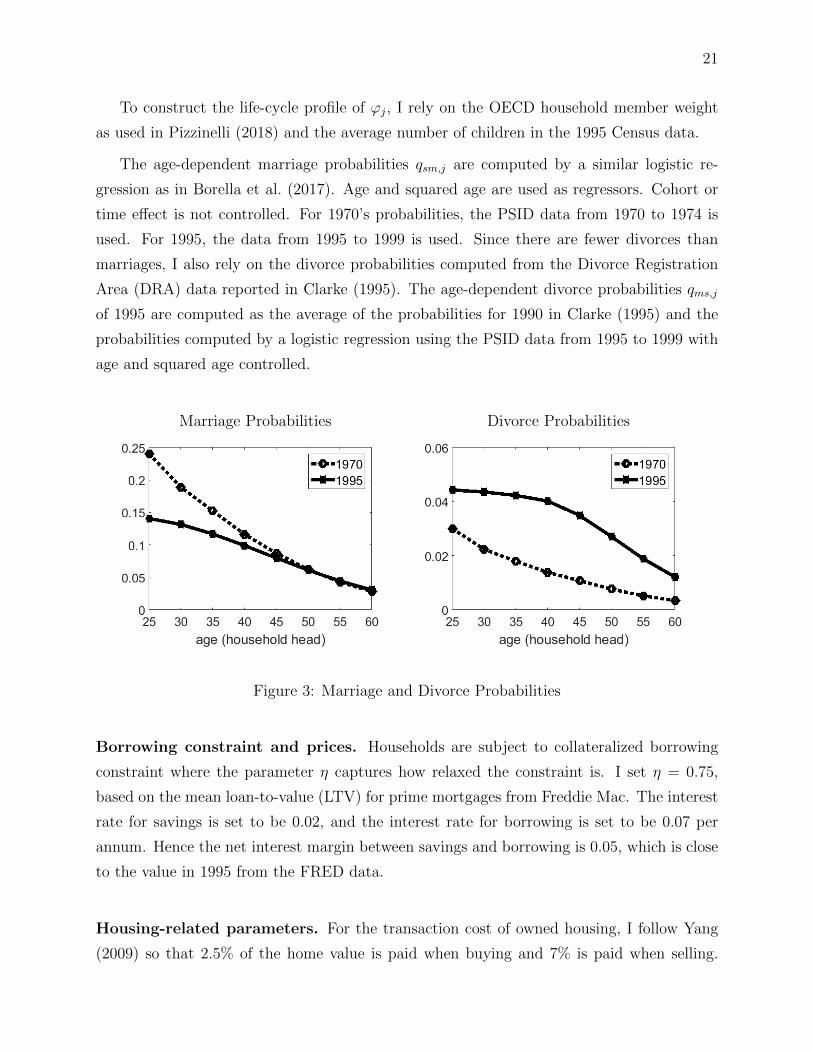
The age-dependent marriage probabilities qsm,j are computed by a similar logistic re-
gression as in Borella et al. (2017). Age and squared age are used as regressors. Cohort or
time effect is not controlled. For 1970’s probabilities, the PSID data from 1970 to 1974 is
used. For 1995, the data from 1995 to 1999 is used. Since there are fewer divorces than
marriages, I also rely on the divorce probabilities computed from the Divorce Registration
Area (DRA) data reported in Clarke (1995). The age-dependent divorce probabilities qms,j
of 1995 are computed as the average of the probabilities for 1990 in Clarke (1995) and the
probabilities computed by a logistic regression using the PSID data from 1995 to 1999 with
age and squared age controlled.
Marriage Probabilities Divorce Probabilities
Figure 3: Marriage and Divorce Probabilities
Borrowing constraint and prices. Households are subject to collateralized borrowing
constraint where the parameter η captures how relaxed the constraint is. I set η = 0.75,
based on the mean loan-to-value (LTV) for prime mortgages from Freddie Mac. The interest
rate for savings is set to be 0.02, and the interest rate for borrowing is set to be 0.07 per
annum. Hence the net interest margin between savings and borrowing is 0.05, which is close
to the value in 1995 from the FRED data.
Housing-related parameters. For the transaction cost of owned housing, I follow Yang
(2009) so that 2.5% of the home value is paid when buying and 7% is paid when selling.

22
Lastly, idiosyncratic house price shock is modeled to be uniform between δ and δ. I set
δ = −0.25, which is close to the average price increase for 10 major U.S. metropolitan areas
(Composite 10) from the Case-Shiller house price index.16 I set δ = 0.15, whose value is
similar to the 2.5th percentile of price change for all states from 1995 to 1999. The common
house price PH is calibrated to match the price-to-rent ratio.
In the decomposition analysis in Section 5, I treat 1970 and 1995 as two steady states
with the same common house price but with different marriage and divorce prospects. When
analyzing the more recent years with changing house prices, I model the common house price
to be a shock similar to Corbae and Quintin (2015). Referring to the price index by Shiller
(2000)17, real home values were relatively stable between 1890 and 2013, except for two
periods. The first exception is from 1920 to 1939, which featured low home values. The
other is the recent housing price boom, which lasted from 1999 until the crisis. Hence, the
common house price is modeled as PHt = PH × zt, where zt is a three-point process
zt ∈ [0.7, 1, 1.3]
with a Markov transition matrix. The support is set from the observation that the average
home values during low times are about 30 percent below the corresponding average during
normal times. Symmetrically, the highest price is set to be 30% higher than the middle
price.18 The transition matrix ΠPH is set as
0.75 0.25 0
0.045 0.91 0.045
0 0.375 0.625
.
This matrix is set based on the following: the middle price is maintained from 1940 to
1995, which corresponds to 11 model periods. Deviations to lowest level are expected to last
for 20 years. Lastly, deviations to highest level are expected to last for about 13 years. Table
2 summarizes the externally set parameters and their sources.
16Given that major metropolitan areas tend to experience sharper housing price increase, I use theaverage of Composite 10 as the upper bound. Composite 10 includes Boston, Chicago, Denver, Las Vegas,Los Angeles, Miami, New York, San Diego, San Francisco, and Washington, D.C.
17http://www.econ.yale.edu/∼shiller/data.htm18This is in line with the observation that the real house price in 2005, which can represent the boom
period, was 30% higher than the price in 1995.

23
Parameter Value Source
Preference
β 0.94 —σ 5.0 —γ 0.5 Keane and Rogerson (2015)
Labor Productivity
χ(j) — Hansen (1993)ρx (ρx) 0.75 (0.73) Fernandez and Wong (2014)σx (σx) 0.4 (0.42) Chang and Kim (2006)
Marriage
nψ 1.34 Fernandez-Villaverde and Krueger (2007)ϕj — Pizzinelli (2018), Census
qsm,j , qms,j — Divorce registration area (DRA) data, PSID
Borrowing Constraint
η 0.75 Freddie Mac mean LTV for prime mortgages(r, rH) (0.02, 0.07) Net interest margin of banks (FRED)
Housing Market
(κb, κs) (0.025, 0.07) Yang (2009)(δ, δ) (-0.25, 0.15) Case-Shiller house price index
Table 2: Externally Set Parameter Values
4.2 Estimated parameters
I estimate the remaining parameters by a limited information Bayesian approach as
in Christiano et al. (2010) and Fernandez-Villaverde et al. (2016). Structural estimation
such as mine has advantages for several reasons. First, we can discipline estimation with
various moments of interest. Since I want my model to be able to account for households’
housing and labor supply decisions, I use the relevant life-cycle profiles of homeownership
rates, housing asset share, and labor force participation rates across singles and married
households. Second, we are able to learn uncertainty associated with parameters in contrast
to calibration. For instance, we can construct a confidence interval or a credible set for each
parameter of interest. We can also quantify the uncertainty in the life-cycle profiles induced
from the parameter estimates. Lastly, one advantage of a Bayesian approach is that we can
explicitly incorporate prior beliefs and combine them with information from the data. As a
special case, a Bayesian inference becomes analogous to a classical inference if one chooses
uniform priors. This will be clear in the following explanation of a limited information
Bayesian procedure.

24
I denote the data moments to match as ψ. The goal is to choose a parameter vector θ
to make the model-simulated moments ψ(θ) be as close as possible to ψ. The approximate
likelihood of ψ is written as
f(ψ|θ) =
(1
2π
)M2
|V (θ0)|−12 × exp
[− 1
2
(ψ − ψ(θ)
)′V (θ0)−1
(ψ − ψ(θ)
)],
where M is the number of moments in ψ and V (θ0) is treated as a known object. To make
this approach adequate, we need at least an approximately consistent estimator for V (θ0).
I use a bootstrap approach with NB bootstrap samples to construct a reasonable estimator
for V (θ0) as
V =1
NB
NB∑b=1
(ψb − ψ)(ψb − ψ)′,
where ψb stands for the moments from the b-th bootstrap sample and ψ is the mean of ψb
for b = 1, . . . , NB. To provide context, there are not many observations for middle-aged and
elderly singles. This procedure will choose to weight more young singles’ moments if they
show lower variance.
The Bayesian posterior of θ conditional on ψ is derived as
f(θ|ψ) =f(ψ|θ)p(θ)f(ψ)
,
where p(θ) denotes the priors on θ and f(ψ) denotes the marginal density of ψ, where
f(ψ) =∫f(ψ|θ)p(θ)dθ. Then I characterize the posterior density using the Random-Walk
Metropolis Hastings sampler with the objective function
g(θ) ≡ log f(ψ|θ) + log p(θ).
The proposal covariance-variance matrix Ωproposal is obtained by multiplying a constant
c to the diagonal matrix Ω whose elements are equal to prior variances, Ωproposal = c × Ω.
As the chain runs, c is updated as in Herbst and Schorfheide (2018) so that the acceptance
rate x gets closer to the target 0.25:

25
c′ = c×(
0.95 + 0.1× e16(x−0.25)
1 + e16(x−0.25)
).
Table 3 shows the parameters to be estimated and their priors. I use the uniform priors
for all the parameters. This reflects that the prior belief does not favor certain values over
the others within the support. This belief would be updated with the curvature provided
by the difference between the moments from the data and those from the model. Given
this prior specification, this procedure can be considered as pseudo-likelihood estimation in
classical inference.
Parameter Distribution Support Description
ζ1 Uniform [1.0, 1.5] Service flow from owned housing (intercept)ζ2 Uniform [0.0, 1.0] Service flow from owned housing (slope)ωuhp Uniform [0.0, 2.0] Utility from home productionγe Uniform [0.5, 1.0] Economies of scale within marriageα Uniform [0.4, 0.9] Aggregator for consumption and housingBs Uniform [10.0, 100.0] Disutility from working (single)Bm Uniform [10.0, 100.0] Disutility from working (married head)
Bm Uniform [10.0, 100.0] Disutility from working (married spouse)φ Uniform [0.0, 2.0] Fixed cost of working (head)
φ Uniform [0.0, 2.0] Fixed cost of working (spouse)
Table 3: Priors
The moments used in this procedure include 1995’s life-cycle profiles for homeowner-
ship rates, housing asset share, and labor force participation rates for single and married
households respectively. For instance, ζ1 is identified from the levels of homeownership rate
whereas ζ2 is identified from the variations in housing asset share over the life-cycle. Without
ωuhp, the model cannot generate married household heads to work more than singles on av-
erage. Hence ωuhp is identified from the gap in the labor force participation between married
heads of households and singles. Due to economies of scale for consumption and housing
services within marriage, investment in housing assets is bigger (and that in non-housing
assets is smaller) for a married couple compared to their single counterpart. γe is identified
from how steeply the housing asset share increases for the married compared to singles. α is
obtained from the overall levels of housing asset share and φ, φ are from the levels of labor
force participation for the single and for the married spouse respectively. Lastly, Bs, Bm, Bm
are identified from how labor supply decreases over the life-cycle. If the disutility of working

26
is high, the decrease in labor supply will be steeper as one gets older.
I obtain the posterior estimates based on 8000 iterations with the average acceptance rate
0.24. Table 4 shows some percentiles from the prior and the posterior distributions. One
advantage of estimation is that we can see the uncertainty associated with each parameter.
By using the 5th percentile and 95th percentile of the posterior draws, we can construct
the 90% credible set for each parameter. In Appendix B, I provide the histogram of each
parameter’s posterior distribution and the cumulative mean of the posterior draws.
Prior PosteriorParameter 5% 50% 95% 5% 50% 95%
ζ1 1.025 1.25 1.475 1.163 1.364 1.480ζ2 0.05 0.5 0.95 0.048 0.341 0.938ωuhp 0.1 1.0 1.9 0.224 1.015 1.858γe 0.525 0.75 0.975 0.558 0.607 0.679α 0.425 0.65 0.875 0.458 0.538 0.593Bs 14.5 55 95.5 33.814 48.670 58.964Bm 14.5 55 95.5 10.731 17.491 46.067
Bm 14.5 55 95.5 19.046 48.318 74.348φ 0.1 1.0 1.9 0.370 1.374 1.932
φ 0.1 1.0 1.9 0.097 0.827 1.736
Table 4: Prior and Posterior Distributions of Estimated Parameters
Note: The columns show 5th, 50th, 95th percentiles of prior and posterior distributions.
4.3 Model fit
Figure 4 shows the model fit for the 1995 data. The model-generated life-cycle profiles
are obtained by using the posterior median, which is shaded in Table 4. The model does a
great job of matching the life-cycle profiles of homeownership rates and housing asset share
depending on marital status. Also, it matches the labor force participation of household
heads well. The model captures the overall life-cycle profile of spousal labor force partici-
pation in the data, even though I do not model many other factors that potentially affect
spousal labor supply. It is meaningful to get the spousal labor supply pattern close to the
data, because I want to experiment with the change in spousal labor supply over time.

27
Homeownership Rate Housing Asset Share
Labor Force Participation (Head) Labor Force Participation (Spouse)
Figure 4: Life-Cycle Profiles: Model vs. Data
Note: Solid line - Model, Dotted line - Data, Blue - Single, Red with circle - Married.
The in-sample fit is also analyzed by posterior predictive checks reported in Figure 5.
I simulate the life-cycle profiles for 50 different posterior draws that are equally-distanced
over the sampler. From Figure 4 based on the posterior median, we observe some gaps be-
tween the model-generated life-cycle profiles and the data’s. The hairlines generated from
the predictive checks allow us to see whether these discrepancies are big or not given the
uncertainty involved. For example, the life-cycle profiles of homeownership rates are quite
precisely estimated whereas there is more uncertainty associated with spousal labor supply
profiles. In addition, the hairlines for housing asset share are more spread out for younger
singles compared to older ones. Hence, the estimation procedure provides us with measures
of uncertainty and some insights that one would not otherwise get with calibration.

28
Figure 5: Predictive Checks of Posterior Draws
Note: Each hairline corresponds to a draw from the posterior distribution.
Lastly, the model is validated with some unmatched moments in Table 5 that are not
included in the sampler.
Variable Model Data
Housing wealth to consumption ratio 2.13 2.3Wealth to income ratio 2.98 3.0-3.5Rent to income ratio 0.23 0.21
Ratio of mean hours worked (Single/Married:Head) 0.81 0.82Ratio of mean hours worked (Married:Spouse/Married:Head) 0.62 0.66
Table 5: Unmatched Moments: Model vs. Data

29
5 Decomposition analysis: 1970 vs. 1995
Given the model and the parameter estimates, I can answer the main question of how
much of the change in marital transition probabilities can account for the change in housing
variables. In addition to this change in marriage and divorce probabilities, other changes
that may be key drivers of households’ housing decisions occurred. The goal of this section
is to quantify the explanatory power of the main channel while controlling for other changes
to affect housing decisions studied in the literature.
5.1 Major changes between 1970 and 1995
(1) Marital transition probabilities
This change is the main channel of interest in this paper. I use the age-dependent marriage
and divorce probabilities as in Figure 3. The baseline life-cycle profiles are generated by using
the marriage and divorce probabilities in 1995. In this decomposition exercise, I feed in the
probabilities in 1970 instead, holding the other things fixed, to see how the housing variables
would have looked under this scenario.
(2) Downpayment constraint
Downpayment constraint was tighter in 1970 compared to 1995. Fisher and Gervais (2011)
point out that the average downpayment in the 1990s was about the two-thirds value of the
average in the 1970s. The parameter governing the tightness of the borrowing constraint is
η. The baseline η is set to be 0.75, which equals 25% downpayment constraint. Instead, I
use η = 0.65 for 1970, which is a similar value as documented in Bullard (2012).
(3) Labor market volatility
The increase in labor market volatility is widely documented as in Fisher and Gervais
(2011) and Santos and Weiss (2013). The parameter associated with earnings risk is σx and
σx. The parameters for 1970 are set to reflect the 40% increase in volatility from 1970 to
1995 as reported in Fisher and Gervais (2011).

30
(4) Spousal labor productivity and fixed cost of working
From 1970 to 1995, the gender wage gap shrank and the labor force participation of
spouses increased substantially. Heathcote et al. (2010) show that the average female wage
increased by about 15% from 1970 to 1995. I set the value of χ(j) in 1970 to reflect this
change while fixing the household head’s χ(j).
However, the labor productivity change is not sufficient to generate the observed change
in spousal labor force participation. Therefore, I also change the parameter φ governing the
fixed cost of working. φ is set to be higher in 1970 so that the average spousal labor force
participation rate matches 0.52 in 1970.
5.2 The effect of each channel
I show how each change affects the housing decisions of single and married households. I
look at the singles’ homeownership rates and the marrieds’ housing asset share, since these
variables changed significantly between 1970 and 1995.
Single: Homeownership Married: Housing Asset Share
Figure 6: The Effect of the Change in Marital Transition Probabilities on Housing Decisions
Note: The black lines are generated from the model using the marriage and divorce probabilitiesin 1995 (baseline). The red lines are obtained by applying the marriage and divorce probabilitiesin 1970, holding the other things identical to the baseline specification.

31
(1) Marital transition probabilities
The red lines in Figure 6 are obtained by changing the marriage and divorce probabilities
to be 1970’s values. I focus on the age groups from 25 to 44 years old since marital transitions
happen relatively early in life. In the left panel of Figure 6, the homeownership rate for young
singles becomes lower under the high marriage probabilities of 1970. It is worth noting that
the gap between the red line and the black line closes as we look at older ages. This captures
that the difference in marriage probabilities between 1970 and 1995 is more conspicuous for
those in their 20s or early 30s. The mechanism that generates this drop in homeownership is
as follows: a single who expects to get married in the near future will refrain from owning a
house due to the transaction costs of selling or resizing. In addition, the prospect of marriage,
which causes a free rider problem with asset pooling, prevents singles from saving.
For the married households, they face lower divorce probabilities in 1970. Due to reduced
idiosyncratic risk of separation, their precautionary savings motive diminishes, which could
reduce the homeownership rate of the married. On the other hand, the housing asset share
increases with lower divorce probabilities. Under the 1970 probabilities, the expected return
on housing goes up as it is less likely to incur transaction costs associated with divorce. As
shown in the right panel of Figure 6, the marrieds’ housing asset share is bigger under 1970’s
likelihood of divorce. The gap between the red line and the black line does not close for the
housing asset share, which reflects that the gap in divorce probabilities do not get narrower
even up to age 44.
I do not use different values for marriage and remarriage probabilities. The remarriage
probabilities reported in the Current Population Reports by Bruno and Glick (1971) are
still higher than the marriage probabilities in 1995. My decomposition analysis captures the
reality consistently in that the married households in 1970 expected remarriage after divorce
to be more likely compared to the households in 1995.
(2) Downpayment constraint
Figure 7 includes the life-cycle profiles generated by each channel considered between
1970 and 1995. The red lines are the same as in Figure 6, showing the effect of marriage and
divorce risk. The blue lines are generated by changing the borrowing constraint to mimic
1970’s environment while holding the other things fixed to 1995’s values.

32
Single: Homeownership Married: Housing Asset Share
Figure 7: The Effect of Each Channel on Housing Decisions
Note: The black lines are generated from the 1995 baseline specification. The red lines are obtainedby only changing the marital transition probabilities to be 1970’s values, holding the other thingsidentical to the baseline specification. The other lines are also obtained by only applying one changeto mimic the 1970’s economy while preserving the others as in 1995; compared to the baseline, theblue lines are with tighter downpayment constraint, the pink lines are with lower labor volatility,and the cyan lines are with lower spousal labor productivity.
The borrowing constraint of interest is b′ ≥ −ηPHh′. With a tighter borrowing con-
straint as in 1970, the singles’ homeownership rates decrease a little whereas the marrieds’
homeownership rates do not change much. However, the average house size for the married
becomes smaller, which results in a decrease in housing asset share. In other words, the
intensive margin adjusts with the financial constraint change although the extensive margin
does not change much for married households. Still, the overall change in housing variables
does not seem to be substantial, with the only change in the loan-to-value parameter η from
0.75 to 0.65. However, this does not rule out the possibility that relaxed credit constraints
have a decisive effect on housing decisions in times of housing price booms or busts. This
will be studied more closely in Section 6.
(3) Labor market volatility
With 40% lower labor market volatility, labor supply increases for all household mem-
bers.19 Furthermore, the level of income in each state changes with diminishing income risk.
19This pattern is the opposite of the data’s pattern since the spousal labor supply was much smaller in1970. The change to capture spousal labor supply correctly is studied below.
33
I check whether the average household labor income is almost identical before and after the
change in volatility. There is only about a 2% increase in the average labor income from this
change, so the essential differences in housing decisions will be mostly from the income risk.
Income risk exerts two opposing forces on homeownership. On the one hand, it is valuable
to delay buying a house until a household can afford it due to the large transaction cost and
income risk. This can lower the homeownership rate, especially for the young who do not
have much wealth. On the other hand, the increase in risk raises the precautionary savings.
This savings can induce more transition from renting to home purchase, thereby increasing
the homeownership rate. Under the baseline parameterization, the latter force dominates
the former so the homeownership rate decreases under lower income risk. This is the case
for both the single and the married.
In terms of housing asset share, the magnitude of change in percentage is smaller than
that of homeownership rate. This is because the reduced precautionary savings motive is
split between housing assets and non-housing assets. If there was only one asset available in
which to invest, say a housing asset, then the decrease in homeownership rate would have
been larger as it would have absorbed all the reduction in precautionary savings motive.
With multiple assets, households can adjust, and therefore the portfolio share of housing
assets does not fall as much.
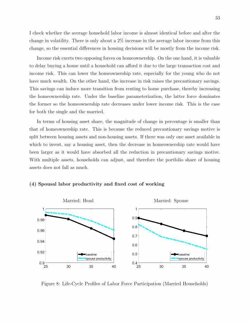
(4) Spousal labor productivity and fixed cost of working
Married: Head Married: Spouse
Figure 8: Life-Cycle Profiles of Labor Force Participation (Married Households)
34
The homeownership rate for both the single and the married are not affected much by
the change in spousal labor force participation. Especially for the married, this is because a
head can increase labor supply as his/her spouse’s labor supply diminishes. Figure 8 shows
how the life-cycle profiles of labor force participation change as I apply the lower spousal
labor productivity χ(j) and the higher fixed cost of working φ. This result is consistent with
the observed pattern in the data that the married heads worked more in 1970 than those in
1995. With the endogenous labor supply, the homeownership rate does not necessarily fall
with a decreased spousal labor supply since the other household member can adjust his/her
labor supply upward.
5.3 Decomposition with the data
In this section, I look at the changes in housing variables from the real-world data between
1970 and 1995 and quantify how much of the change can be accounted for by the change in
marital transition probabilities.
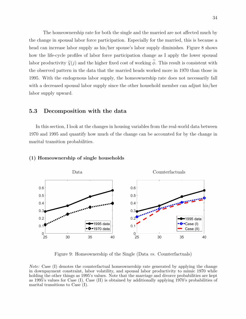
(1) Homeownership of single households
Data Counterfactuals
Figure 9: Homeownership of the Single (Data vs. Counterfactuals)
Note: Case (I) denotes the counterfactual homeownership rate generated by applying the changein downpayment constraint, labor volatility, and spousal labor productivity to mimic 1970 whileholding the other things as 1995’s values. Note that the marriage and divorce probabilities are keptas 1995’s values for Case (I). Case (II) is obtained by additionally applying 1970’s probabilities ofmarital transitions to Case (I).

35
The homeownership rate of single households was lower in 1970 compared to that in
1995 as shown in the left panel of Figure 9. The right panel of Figure 9 includes two coun-
terfactual life-cycle profiles of homeownership. First, the blue dotted line is generated by
applying all the changes except for the marriage and divorce probabilities. In other words,
the marital transition probabilities are kept as 1995’s values, whereas the downpayment con-
straint, labor volatility, and spousal labor productivity are set to reflect 1970’s environment.
All the changes except for the marital transition probabilities induce homeownership to fall
compared to the baseline in 1995. However, this does not generate a sufficient drop to match
that which is observed in the data, especially for young households in their 20s. The red
dashed line in Figure 9 is obtained once I additionally incorporate 1970’s marriage and di-
vorce probabilities. As younger singles refrain from buying a house under the likelihood of
marriage in 1970, the homeownership rate drops further from the blue dotted line.
Data CounterfactualsAge % Change Case (I) Case (II)
25 - 29 -61% -24% -56%30 - 34 -30% -11% -16%35 - 39 -29% -16% -19%40 - 44 -30% -18% -21%
Average -38% -17% -28%
Table 6: Homeownership of the Single (Data vs. Counterfactuals)
Table 6 quantifies the change in percentage, taking the year 1995 as the benchmark.
For instance, the homeownership of single households of age 25-29 was 61% lower in 1970
compared to 1995. The third column, Case (I), shows the counterfactual homeownership
rates generated by applying all the changes except for the marriage and divorce probabilities.
By taking the average over the age groups from 25 to 44 years, this specification generates
the 17% drop in homeownership compared to the baseline. In summary, 45% of the change
observed in the data can be explained by the combined change captured by Case (I).
The last column, Case (II), shows the values obtained by additionally applying 1970’s
marriage and divorce probabilities to Case (I). This specification generates the average of
28% drop in homeownership rate from age 25 to 44. In other words, 29% of the change can
be accounted for by the change in marriage and divorce probabilities. The change in marital
transitions seems to be quantitatively of comparable importance to the combined effect of

36
borrowing constraints, earnings risk, and spousal productivity.
(2) Housing asset share of married households
Figure 10 shows that the housing asset share was higher in 1970 than in 1995. The blue
line from the changes except for the marital transition probabilities shows a small decrease
in the housing asset share. Since the reduced precautionary savings motive is split between
housing asset and non-housing asset, the housing asset share does not fall as much as the
homeownership would fall. On the other hand, the reduction of divorce risk induces married
households to tilt their portfolio towards housing assets. This change is reflected in the red
dashed line of Figure 10.
Data Counterfactuals
Figure 10: Housing Asset Share of the Married (Data vs. Counterfactuals)
Note: Case (I) denotes the counterfactual housing asset share generated by applying the changein downpayment constraint, labor volatility, and spousal labor productivity to mimic 1970 whileholding the other things as 1995’s values. Note that the marriage and divorce probabilities are keptas 1995’s values for Case (I). Case (II) is obtained by additionally applying 1970’s probabilities ofmarital transitions to Case (I).
Table 7 summarizes the change in percentage of housing asset share. Without the change
in marital transition probabilities, the average change has the negative sign, which is the
opposite of what we observe in the data. However, once incorporating 1970’s marriage and
divorce probabilities, the direction of change becomes consistent with the data. With all
the changes applied, 31% of the observed change in portfolio share can be generated. This

37
decomposition analysis emphasizes that the change in marital transition probabilities is an
important risk factor when it comes to understanding the change in housing decisions.
Data CounterfactualsAge % Change Case (I) Case (II)
25 - 29 +17% -3% +8%30 - 34 +11% -3% +7%35 - 39 +18% -2% +5%40 - 44 +6% -11% -6%
Average +13% -3% +4%
Table 7: Housing Asset Share of the Married (Data vs. Counterfactuals)
6 Recent experiences in the housing market
The change in marital transition probabilities is shown to help account for the change in
housing variables between 1970 and 1995. The question in this section is whether marital
transitions have continued to change and, if so, whether they are still useful to understand
the changing housing variables in recent years. In the previous decomposition analysis, the
two years — 1970 and 1995 — were deliberately chosen because while the real house prices
were similar in levels, the marital transition probabilities were different. This allows us to
study the effect of marital transition probabilities while controlling for the house price, which
is a confounding factor. Furthermore, cohabitation was prevalent neither in 1970 nor 1995,
which justified treating only the legally married households as the married.
However, if we want to study the change in housing variables in more recent periods, it
is inevitable to consider the housing price boom, bust, and recovery. Over these periods,
there have also been major changes in credit constraints, wages, and households’ beliefs on
future housing prices. The main analysis of this section is on whether the likelihood of
marital transitions plays a role in explaining housing decisions over time, considering several
factors that characterize the recent experiences in the housing market. Also, as cohabitation
has become more common these days, it is worth looking at whether there is any difference
between legally married households and cohabiting couples in terms of housing decisions. The
last subsection serves as a robustness check by categorizing cohabiting couples as married
households.

38
6.1 Major changes over time
(1) Marital transition probabilities
Figure 11 overlays the marriage and divorce probabilities in 2007 on those in both 1970
and 1995. The marriage probabilities for young singles in their 20s or 30s continued to fall.
In addition, the divorce probabilities fell for young singles. From 1995 to 2007, marital tran-
sition probabilities moved in the same direction. This is opposite of that which happened
between 1970 and 1995; marriage probabilities fell while divorce probabilities increased. For
the subsequent analysis, I assume that the marriage and divorce probabilities for the year
2007 and those for the years after 2007 are the same.
Marriage Probabilities Divorce Probabilities
Figure 11: Marriage and Divorce Probabilities
(2) Housing prices and beliefs on price appreciation
This paper considers the housing prices to be exogenous, which does not analyze what
drives the substantial price changes over time. To make housing prices vary, I use the three-
point process PHt = PH × zt , as described in Section 4, which is similar to Corbae and
Quintin (2015) in which
zt ∈ [0.7, 1.0, 1.3], ΠPH =
0.75 0.25 0
0.045 0.91 0.045
0 0.375 0.625
.

39
Let’s first look at the life-cycle profiles of homeownership rates from applying the shock
above. Starting from the steady state of 1995, I feed in the house price series so that the
highest price hits the economy only in 2005. The blue dotted lines in Figure 12 are obtained
in the model period 2005.20 The model cannot simulate households to own more housing
while facing the more expensive price. The homeownership rates of both the single and the
married are much lower compared to what is observed in the 2007 data. Since housing prices
are at their highest levels, they are expected to fall. Hence, households do not invest in
housing assets unless they expect the asset price to rise more.
Single Married
Figure 12: Homeownership at the House Price Boom (Data vs. Model)
Note: The black lines are drawn with the 2007 Survey of Consumer Finances data, which representsthe housing price boom. The blue lines are obtained from the model by applying the stochastichouse price shock as follows: starting from the steady state of 1995, the house price series is fed sothat the highest price hits the economy in 10 years. The blue lines stand for the homeownershipat this boom period.
Hence, I model that households could expect house price appreciation while facing a
higher house price in a similar vein to Kaplan et al. (2017). Specifically, I incorporate an
additional shock of households’ beliefs on house price appreciation. Belief shock of future
appreciation ot is modeled as the two-state process where ot ∈ 0, ε = 0.6.21 With this
additional shock, the future house price is expected to be PHt+1 × (1 + ot+1). The transition
20When I conduct an analysis with (simulated) housing asset share, the results are qualitatively similar.Hence, the results with homeownership rates are reported.
21The value of ε is consistent with Case et al. (2012), where survey expectations on annual housing pricegrowth are reported to be between 6 and 15 percent in four metropolitan areas. ε = 0.6 is translated as 12percent increase per annum.

40
matrix of ot is set to be
Πo ≡
[π00 π0ε
πε0 πεε
]=
[0.85 0.15
0.5 0.5
].
In other words, given ot = 0, households expect the future price to bePHt+1 with probability 0.85
PHt+1 × (1 + ε) with probability 0.15.
Households are not likely to be optimistic about additional future price appreciation.
The expected duration of not being optimistic is about 30 years.
On the other hand, given ot = ε, households expect the future price to be
PHt+1 with probability 0.5
PHt+1 × (1 + ε) with probability 0.5.
Once a household becomes optimistic, that is ot = ε, then the household expects future
price appreciation PHt+1 × (1 + ε) with a half probability. The expected duration of being
optimistic is 10 years, which is close to the length of the recent housing boom-bust episode
in the 2000s. Physical environment at period t such as budget constraint does not change
with ot. All the change lies in the expectation about the future house price.
Given this additional shock, I define a new state variable τt ≡ (PHt , ot). This augmented
shock τt can take 6 possible values. τt ∈ (pH1 , 0), (pH1 , ε), (pH2 , 0), (pH2 , ε), (p
H3 , 0), (pH3 , ε) ≡
τ1,0, τ1,ε, τ2,0, τ2,ε, τ3,0, τ3,ε. The transition matrix is
Πτ = ΠPH⊗Πo =
0.75 0.25 0.0
0.045 0.91 0.045
0.0 0.375 0.625
⊗[
0.85 0.15
0.5 0.5
]=
0.638 0.113 0.213 0.038 0 0
0.375 0.375 0.125 0.125 0 0
0.038 0.007 0.774 0.137 0.038 0.007
0.023 0.023 0.455 0.455 0.023 0.023
0 0 0.319 0.056 0.531 0.094
0 0 0.188 0.188 0.313 0.313
.
I extend the previous model with an additional state τt and its transition matrix Πτ . The
expected value should be carefully computed, taking into account the stochastic nature of
τt+1 given τt. I apply the sequence of shocks (PHt , ot) in Table 8. There is empirical evidence

41
such as Piazzesi and Schneider (2009) and Landvoigt (2017) supporting the optimistic beliefs
of households for house price appreciation. I set the belief shock to hit both 2000 and 2005,
whereas the highest house price shock hit 2005 only. Standing at the baseline year 1995, the
ex-ante probability of this particular realization of shocks is close to 0.05%. In this regard,
this simulation represents a tail event similar to the boom-bust episode of the 2000s.
(3) Wage and credit constraints
In addition to the change in housing prices and households’ beliefs, I consider the simul-
taneous change in wages and credit constraints during the boom as in Kaplan et al. (2017).
I set the wage to be 7% higher in both 2000 and 2005 compared to the baseline wage in 1995.
This change is similar to the change observed in the median weekly real earnings for wage
and salary workers.22 The 7% wage increase is a little smaller than the change in average
male wage reported in Heathcote et al. (2010), which is about a 10% increase.
For credit constraints, I consider the following changes. First of all, the downpayment
constraint is relaxed by changing (1− η) to be 0.15 in 2005 compared to 0.25 in 1995. Then
the value for 2000 is taken to be 0.2, the average of the two. Second, the borrowing interest
rate rH is reduced to be 0.05 per annum and the savings interest rate r is set to be 0.015 in
2005. The values for 2000 are again taken to be the average of the 1995 value and the 2005
value. This change is consistent with the decrease in the fixed rate for a 30-year mortgage
and the decrease in the net interest margin.
Changes 1995 2000 2005 2010Housing price shock PH
t pH2 pH2 pH3 pH2Belief shock of appreciation ot 0 ε ε 0
Wage w 1.0 1.07 1.07 1.0Downpayment constraint (1− η) 0.25 0.2 0.15 0.25
Borrowing interest rate rH 0.07 0.06 0.05 0.07Savings interest rate r 0.02 0.018 0.015 0.02
Likelihood of marital transitions baseline marriage ↓, divorce ↓
Table 8: The Sequence of Changes Over Time
Note: pH2 is the middle house price and pH3 is the high house price. The wage is normalized so thatthe value in 1995 is 1.0. The interest rates are reported in annual terms.
22This is based on LES1252881600Q series from the FRED.

42
6.2 The effect of each channel: during boom
Single Married
Figure 13: The Effect of Each Channel on Homeownership (During Boom)
Note: The black lines are drawn with the 2007 Survey of Consumer Finances data, which representsthe housing price boom. The other lines are obtained by applying the sequence of changes overtime as in Table 8.
The blue lines in Figure 13 (identical to Figure 12) show that the change in housing
prices alone is insufficient to generate the homeownership increase observed in the data for
both the single and the married.
(1) Marital transition probabilities
The pink lines are obtained by changing the probabilities of marriage and divorce to be
the 2007 values as in Figure 11. The marriage probabilities continued to fall for the young
households and so did the divorce probabilities. As the singles are less likely to get married,
their homeownership rate increases. The average homeownership rate from age 25 to 44
increases by 6.8%. As seen in Figure 13, the effect of marital transitions is larger for younger
singles. To be specific, there is about a 20% increase for the age group of 25-29 years and a
5% increase for 30-34 years. Hence, this channel contributes to narrow the gap between the
baseline and the 2007 data for young singles.
On the other hand, the marrieds’ homeownership rate decreases with the decrease in
divorce probabilities. The reduced precautionary savings motive exerts downward pressure
on married couples to decrease their homeownership. There is about a 3% decrease in the

43
average homeownership from 25 to 44 years. The recent marital transition probabilities
slightly widen the gap between the baseline and the 2007 data for married households.
(2) Wage and credit constraints
The cyan line in Figure 13 is obtained by changing wage and credit constraints as in
Table 8. With these changes, the homeownership rate increases. The following numbers
show the change in percentage of homeownership rate for each age group; the cyan lines are
compared with the pink lines from applying the recent marital transition probabilities. The
first number is for 25-29 years and the last one is for 40-44 years.
For the single: +10.9%, +9.3%, +2.3%, +2.4%
For the married: +32.9%, +14.3%, +12.2%, +9.2%
The higher wage and the relaxed credit constraints (lower interest rates, lower downpay-
ment requirements) induce homeownership to increase for both singles and married house-
holds, the increase in percentage for the latter being much bigger. As married households are
more likely to buy a house with the joint asset and labor income compared to singles, they
react more strongly once the conditions are improved to make housing affordable. Although
better wage and credit constraints increase the homeownership rate, they are still insufficient
to match the homeownership rate in the 2007 data.
(3) Belief on house price appreciation
Lastly, I add the shock on beliefs about future price appreciation. When doing so, the
homeownership rate becomes similar in level to what is observed in the real-world data. It
is worth noting that it is not only the effect of optimism on price appreciation. Without
the wage increase and the lax credit constraints, the increase in homeownership from mere
optimism is much smaller than the red lines in Figure 13. Thus, to enable households to
afford more housing, we need beliefs about housing price appreciation in addition to changes
in labor income and borrowing capacity. A similar point is also made in Kaplan et al. (2017).
To sum up, although the magnitude of change is smaller compared to that in the past
(1970 vs. 1995), the change in likelihood of marital transitions still increases homeownership

44
among the single and decreases homeownership among the married. However, the unprece-
dented changes in wages, credit constraints, and beliefs of appreciation, coupled with a boom
in housing prices, played a tremendous role in generating a surge in the homeownership rate.
For the married, these changes during the boom seemed to mask the trend of decreasing
homeownership rates induced by the marital transitions. In contrast, the change in marriage
probabilities contributes to replicate the homeownership increase for young singles even when
the housing prices were expensive.
6.3 Homeownership over recent years
So far, I have shown that my model can generate the changes in homeownership during
the boom with the associated changes in prices, credit constraints, and beliefs on housing
price increase. In this subsection, I look at the periods after the boom-bust episode when
the real house price became similar to 1995’s level again. Figure 14 shows the time series of
real home price index. For the recovery periods (2010 and 2013),23 the house price is set to
be back to the middle value pH2 . In addition, all the other parameters are set to be 1995’s
values except for the marriage and divorce probabilities.
Figure 14: Real Home Price Index in the Recent Years
Note: The real home price index is the US Standard & Poors/Case-Shiller index. This figure is taken from
Corbae and Quintin (2015).
23 The most recent data available is the 2016 SCF. But I do not include this period because the real homeprice index seems to show another increasing trend.

45
Figure 15 shows the life-cycle profiles of homeownership over time from the data and
from the model simulation. The upper panels are obtained from the data. In 2007, a period
representative of the housing price boom, the married households’ homeownership rate was
higher compared to the benchmark year 1995. The increase in homeownership is not so con-
spicuous for singles except for one age group (30-34 years). Following Glover et al. (2017),
I treat the average life-cycle profiles of 2010 and 2013 as representing the recovery periods
after the bust. During the recovery periods, the homeownership rate of married households
is even lower than 1995, especially for those in their 20s. But for singles of the same age
group, the fall in homeownership rate is not observed.
Single: Data Married: Data
Single: Model Married: Model
Figure 15: Homeownership Over Time (Data vs. Model)
The bottom panels are obtained by the simulation applying the changes in Table 8. The

46
red dashed lines are from the model period 2005 and the blue dotted lines are from the model
period 2010. From the simulation, the only difference between 1995 (the baseline year) and
2010 lies in marriage and divorce probabilities. For the married households, the homeown-
ership rate decreases as marriage and divorce become less likely. This direction of change
is consistent with what we observe in the data. If there were only the change in marital
transition probabilities, the homeownership of married households would have been decreas-
ing over time. However, with the other changes associated with surging housing prices,
the homeownership rate increased significantly during the boom. For single households, the
model generates a slight increase in homeownership in the recovery period compared to 1995.
As young singles are less likely to get married, they purchase housing instead of waiting until
they get married. In the data representing the recovery period, the homeownership rate of
singles aged 25 to 34 did not fall, which is in contrast to the decrease in ownership for those
aged 35 and older. This may be due to the upward pressure resulting from the reduced
marriage probabilities.
Married SinglePeriod Data Model Data Model
1995 0.72 0.70 0.42 0.41Mid 2000s 0.78 0.78 0.45 0.44
2010 0.68 0.68 0.40 0.44
Table 9: The Average Homeownership Rate Over Time (Average of 25-44 Years)
Table 9 summarizes the average homeownership rate over time, focusing on the house-
holds aged 25-44 years old. For married households, the over-time change in homeownership
from the model tracks with the patterns from the data well. The change in the likelihood of
marriage and divorce helps replicate the decreasing homeownership among the young mar-
ried households. But the changes during the boom (mid 2000s) seem to have masked this
decreasing trend in homeownership.
For singles, the model is able to generate the increase in homeownership from 1995 to
the mid 2000s. But the model predicts that the homeownership rate will maintain the same
average in 2010, which is inconsistent with the decrease observed in the data. There may be
other factors that exert a downward force on singles’ homeownership rate during the recovery
period. One potential factor could be the heightened fear of unemployment, as pointed out
in Den Haan et al. (2015). This fear would repress the desire to spend or to save in an illiquid

47
asset, leading to a lower homeownership rate. This remains a question for future research.
6.4 Robustness check: cohabitation
The rate of cohabitation more than doubled between 1995 and 2010. According to the
Current Population Survey, 7% of adults of age 30-44 cohabited in 2010 compared to 3%
who did so in 1995. In all the analysis prior to this subsection, only the legally-married
households are considered to be married. The concern is whether legal marriage in recent
years is mere labeling; if legally married households and cohabiting couples are qualitatively
similar in terms of housing decisions, it might be misleading to categorize cohabiting couples
as single households. In the following subsections, I look at the two data sources with the
information on cohabitation and see whether the previous analysis is still robust regardless
of how cohabiting couples are categorized.
(1) From SCF data
Without Cohabitors (Previous Analysis) With Cohabitors
Figure 16: The Marrieds’ Homeownership With and Without Cohabitors
Note: The line for 1995 data is drawn with legally married households only — the same baselineto help comparison.
Figure 16 shows the homeownership rate for married households, where “being mar-
ried” is differently defined. In the left panel, I only treat a household with a legal spouse
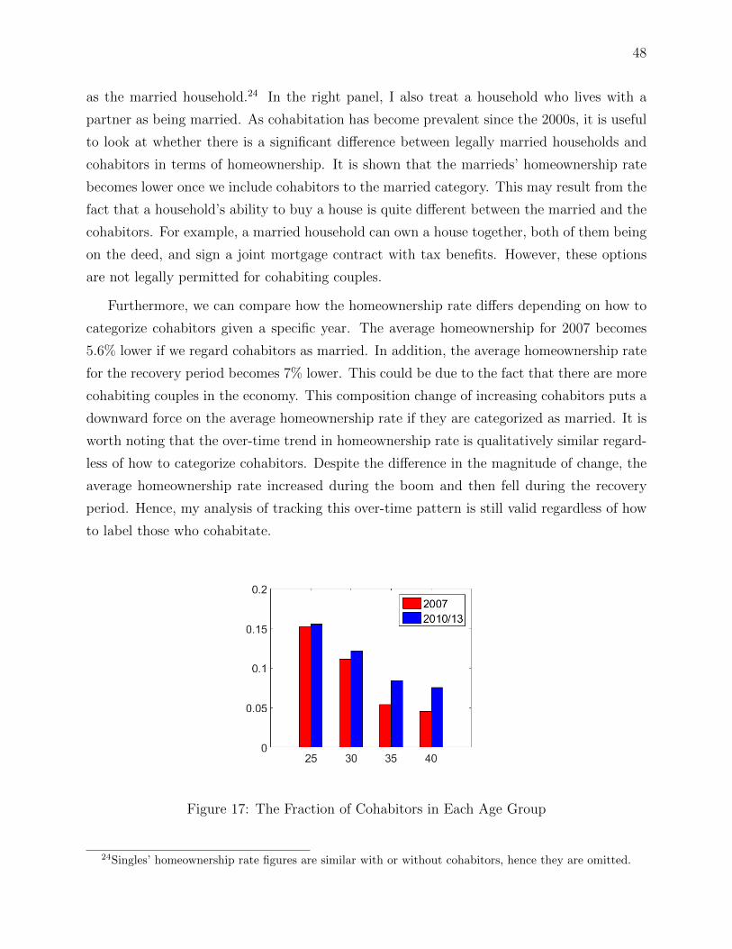
48
as the married household.24 In the right panel, I also treat a household who lives with a
partner as being married. As cohabitation has become prevalent since the 2000s, it is useful
to look at whether there is a significant difference between legally married households and
cohabitors in terms of homeownership. It is shown that the marrieds’ homeownership rate
becomes lower once we include cohabitors to the married category. This may result from the
fact that a household’s ability to buy a house is quite different between the married and the
cohabitors. For example, a married household can own a house together, both of them being
on the deed, and sign a joint mortgage contract with tax benefits. However, these options
are not legally permitted for cohabiting couples.
Furthermore, we can compare how the homeownership rate differs depending on how to
categorize cohabitors given a specific year. The average homeownership for 2007 becomes
5.6% lower if we regard cohabitors as married. In addition, the average homeownership rate
for the recovery period becomes 7% lower. This could be due to the fact that there are more
cohabiting couples in the economy. This composition change of increasing cohabitors puts a
downward force on the average homeownership rate if they are categorized as married. It is
worth noting that the over-time trend in homeownership rate is qualitatively similar regard-
less of how to categorize cohabitors. Despite the difference in the magnitude of change, the
average homeownership rate increased during the boom and then fell during the recovery
period. Hence, my analysis of tracking this over-time pattern is still valid regardless of how
to label those who cohabitate.
Figure 17: The Fraction of Cohabitors in Each Age Group
24Singles’ homeownership rate figures are similar with or without cohabitors, hence they are omitted.

49
(2) From PSID data
In this subsection, I look at the marriage and divorce probabilities depending on how
cohabitors are categorized. In the PSID data, there are two variables related to marital sta-
tus. Taking the 2007 PSID as an example, variable ER36023 asks the legal marital status
whereas ER41039 asks marital status where no distinction is made between those legally
married and those who merely cohabitate. I construct the age-dependent marriage and di-
vorce probabilities using these two different variables.
Marriage Probabilities Divorce Probabilities
Figure 18: Marriage and Divorce Probabilities with and without Cohabitors
The top panels in Figure 18 show the marriage and divorce probabilities depending on
how to categorize cohabitors. The divorce probabilities become higher once we include
cohabitors among the married. So we can see that the young cohabitors are more likely to
separate than the legally married. The marriage probabilities become lower once we include

50
cohabitors. This indicates that the transition from single to either married or cohabiting
is less likely than the one from single or cohabiting to married. The bottom panels show
how the likelihood of marital transitions changed over time. The black lines are based on
labeling only the legally married as married households. The blue dashed lines are from
adding cohabitors to the married category. Regardless of the categorization, the recent
trend of falling marriage and divorce probabilities is kept.
7 Concluding remarks
Owner-occupied housing is the most widely held assets and an important source of indi-
vidual and national wealth. Many countries have attempted to boost home purchasing by
implementing policies such as mortgage subsidies and tax benefits. To assess the effective-
ness of such policies, it is crucial to study the drivers for households’ housing decisions. This
paper argues that the evolving likelihood of marriage and divorce is an essential factor in
accounting for how housing decisions have changed in the United States.
I first look at two years — 1970 and 1995 — when the real house prices were similar in
level but the marriage and divorce probabilities differed substantially. Comparing these two
years, the micro data shows that the singles’ homeownership increased for all age groups
and the young marrieds’ housing asset share decreased. I conjecture that these changes in
housing variables could be affected by the change in the likelihood of marital transitions.
A single who is likely to get married soon will wait to buy a house with a spouse because
it is costly to sell or resize a house. Furthermore, the prospect of marriage creates a free
rider problem that discourages singles from saving, which makes it unlikely for them to be
homeowners. For a married couple, a high probability of divorce will prevent them from
investing in housing because it is more difficult to split a house than liquid assets.
To quantify what fraction of the observed change in homeownership and housing asset
share can be explained by the change in marital transitions, I build a life-cycle model of
single and married households that face exogenous age-dependent marital transition shocks.
In times of getting married or divorced, a substantial transaction cost is modeled to arise
because housing is a highly idiosyncratic investment, and a marital status change would make
the house owned prior to the change no longer suitable. In addition, the model includes the
features to incorporate the changes in borrowing constraints, earnings risk, and spousal
productivity.

51
I estimate the parameters of the model by a limited information Bayesian method to
match the moments from 1995’s cross-section data. Then I conduct a decomposition analysis
comparing 1970 to 1995 as two steady states with different marriage and divorce probabilities.
I find that the change in the likelihood of marital transitions accounts for 29% of the increase
in the homeownership rate of singles. This fraction is substantial given that the changes in
downpayment requirements, earnings risk, and spousal labor productivity jointly replicate
45% of the change. Furthermore, the model can only reproduce the decline in housing asset
share if the changes in marital transitions are included. In their absence, the other drivers
predict an increase in this share, again demonstrating the crucial importance of this channel
for observed trends in households’ housing decisions.
I then extend my analysis to study whether the ongoing change in marital transitions still
plays a role in explaining housing decisions in recent years. To do so, one must inevitably
incorporate the dramatically changing house prices as seen in the boom-bust episode of the
2000s. Hence, I simulate the homeownership rates with the changes in marital transitions,
house prices, beliefs on appreciation, credit constraints, and wages. These changes are set
to mimic the recent experiences in the housing market. The decrease in both marriage and
divorce probabilities increases the singles’ homeownership rate by 6.8%, but it decreases the
marrieds’ homeownership rate by 3.2%. The changes in credit constraints, wages, and beliefs
on appreciation were often suggested as drivers for the homeownership increase during the
boom, which is also supported by my paper. It is worth noting that the change in marital
transitions contributes to replicate the homeownership increase for young singles even when
housing prices were expensive.
This paper sheds light on how underlying demographic changes have shaped households’
housing decisions, which could be of interest to policymakers. For instance, the Trump
administration suggested a new tax law that will reduce the number of people who can
claim the mortgage interest deduction. This policy may have very different impacts across
households depending on their marital stability and their risk of a status change. Also, the
trend of decreasing marriages puts upward pressure to the singles’ homeownership. As a
result, the change in mortgage interest deductability may be more detrimental to singles
than it is intended to be.
Lastly, since marital transitions and housing decisions are complex problems in life, my
model abstracts from some interesting dimensions to explore, including strategic interactions
within marriage. In other words, my model is a measurement device to see how much the
likelihood of marital transitions account for the change in housing decisions while ruling

52
out disagreement between married spouses. As a first pass, this model is still meaningful
to account for the increase in the singles’ homeownership and the decrease in the marrieds’
housing asset share. How these within-group changes in housing decisions are affected by
the prospect of marriage and divorce has not been quantified in the literature. However, the
current model is not sufficient to study, for example, how divorced males and females differ
in their decisions and outlooks and how these discrepancies affect the joint decision during
the marriage. Incorporating intra-household bargaining or collective decision making would
be an interesting avenue for future research.

53
References
Blundell, Richard, Luigi Pistaferri, and Ian Preston, “Imputing Consumption in the
PSID Using Food Demand Estimates in the CEX,” 2005. Stanford University Working
Paper.
, , and , “Consumption Inequality and Partial Insurance,” American Economic Re-
view, 2008, 98, 1887–1921.
Borella, Margherita, Mariacristina De Nardi, and Fang Yang, “Marriage-related
Policies in an Estimated Life-Cycle Model of Housholds’ Labor Supply and Savings for
Two Cohorts,” 2017. Working Paper.
Brown, Meta and Christopher J. Flinn, “Family Law Effects on Divorce, Fertility and
Child Investment,” 2011. Working Paper.
Bruno, Rosalind R. and Paul C. Glick, “Social and Economic Variations in Marriage,
Divorce, and Remarriage: 1967,” Current Population Series 223, U.S. Bureau of the Census
1971.
Bullard, James, “The Aftermath of the Housing Bubble,” 2012. Presentation at Housing in
America: Innovative Solutions to Address the Needs of Tomorrow, The Bipartisan Policy
Center, St. Louis.
Case, Karl E., Robert J. Shiller, and Anne K. Thompson, “What Have They Been
Thinking? Homebuyer Behavior in Hot and Cold Markets,” Brookings Papers of Economic
Activity, 2012, 2, 265–298.
Chang, Yongsung and Sun-Bin Kim, “From Individual to Aggregate Labor Supply: A
Quantitative Analysis Based on a Heterogeneous Agent Macro Economy,” International
Economic Review, 2006, 47, 1–27.
Christiano, Lawrence J., Mathias Trabandt, and Karl Walentin, “DSGE Models
for Monetary Policy Analysis,” in B.M. Friedman and Michael Woodford, eds., Handbook
of Monetary Economics, Vol. 3, Elsevier, 2010, pp. 285–367.
Clarke, Sally, “Advance Report of Final Divorce Statistics, 1989 and 1990,” Monthly Vital
Statistics Report, 1995, 43, 1–31.

54
Cocco, Joao F., “Portfoilo Choice in the Presence of Housing,” Review of Financial Studies,
2005, 18, 535–567.
Corbae, Dean and Erwan Quintin, “Leverage and the Foreclosure Crisis,” Journal of
Political Economy, 2015, 123, 1–65.
Cubeddu, Luis and Jose-Vıctor Rıos-Rull, “Families as Shocks,” Journal of the Euro-
pean Economic Association, 2003, 1, 671–682.
Diaz, Antonia and Maria Jose Luengo-Prado, “On the User Cost and Homeowner-
ship,” Review of Economic Dynamics, 2008, 11, 584–613.
Favilukis, Jack, Sydney C. Ludvigson, and Stijn Van Nieuwerburgh, “The Macroe-
conomic Effects of Housing Wealth, Housing Finance, and Limited Risk Sharing in General
Equilibrium,” Journal of Political Economy, 2017, 125, 140–223.
Fernandez, Raquel and Joyce Wong, “Divorce Risk, Wages and Working Wives: A
Quantitative Life-Cycle Analysis of Female Labour Force Participation,” The Economic
Journal, 2014, 124, 319–358.
Fernandez-Villaverde, Jesus and Dirk Krueger, “Consumption Over the Life Cycle:
Facts From Consumer Expenditure Survey Data,” Review of Economics and Statistics,
2007, 89, 552–565.
, J.F. Rubio-Ramırez, and Frank Schorfheide, “Solution and Estimation Methods for
DSGE Models,” in John B. Taylor and Harald Uhlig, eds., Handbook of Macroeconomics,
Vol. 2, Elsevier, 2016, pp. 527–724.
Fischer, Marcel and Natalia Khorunzhina, “Housing Decision Under Divorce Risk,”
2016. Working Paper.
Fisher, Jonas D. M. and Martin Gervais, “Why Has Home Ownership Fallen Among
The Young?,” International Economic Review, 2011, 52, 883–912.
Flavin, Marjorie and Takashi Yamashita, “Owner-Occupied Housing and the Compo-
sition of the Household Portfolio,” American Economic Review, 2002, 92, 345–362.
Friedberg, Leora, “Did Unilateral Divorce Raise Divorce Rates? Evidence from Panel
Data,” American Economic Review, 1998, 88, 608–627.

55
Gallin, Joshua, “The Long-Run Relationship Between House Prices and Rents,” Real
Estate Economics, 2008, 36, 635–658.
Glover, Andrew, Jonathan Heathcote, Dirk Krueger, and Jose-Vıctor Rıos-Rull,
“Intertemporal Redistribution in the Great Recession,” 2017. Working Paper.
Grossman, Sanford J. and Guy Laroque, “Asset Pricing and Optimal Portfolio Choice
in the Presence of Illiquid Durable Consumption Goods,” Econometrica, 1990, 58, 25–51.
Haan, Wouter J. Den, Pontus Rendahl, and Markus Riegler, “Unemployment
(Fears) and Deflationary Spirals,” 2015. Working Paper.
Hansen, G. D., “The Cyclical and Secular Behaviour of the Labor Input: Comparing
Efficiency Units and Hours Worked,” Journal of Applied Econometrics, 1993, 8, 71–80.
Heathcote, Jonathan, Fabrizio Perri, and Giovanni L. Violante, “Unequal We Stand:
An Empirical Analysis of Economic Inequality in the United States, 19672006,” Review of
Economic Dynamics, 2010, 13, 15–51.
Herbst, Ed and Frank Schorfheide, “Tempered Particle Filtering,” Journal of Econo-
metrics, 2018, Forthcoming.
Jeske, Karsten, Dirk Krueger, and Kurt Mitman, “Housing, Mortgage Bailout Guar-
antees and the Macro Economy,” Journal of Monetary Economics, 2013, 60, 917–935.
Kaplan, Greg and Giovanni L. Violante, “A Model of the Consumption Response to
Fiscal Stimulus Payments,” Econometrica, 2014, 82, 1199–1239.
, Kurt Mitman, and Giovanni L. Violante, “The Housing Boom and Bust: Model
Meets Evidence,” 2017. Working Paper.
Keane, Michael and Richard Rogerson, “Reconciling Micro and Macro Labor Supply
Elasticities: A Structural Perspective,” Annual Review of Economics, 2015, 7, 89–117.
Kuhn, Moritz, Moritz Schularick, and Ulrike I. Steins, “Income And Wealth In-
equality In America, 1949-2013,” 2017. Working Paper.
Landvoigt, Tim, “Housing Demand During the Boom: The Role of Expectations and
Credit Constraints,” Review of Financial Studies, 2017, 30, 1865–1902.
56
Love, David A., “The Effect of Marital Status and Children on Savings and Portfolio
Choice,” Review of Financial Studies, 2010, 23, 385–432.
Low, Hamish, Costas Meghir, and Luigi Pistaferri, “Wage Risk and Employment
Risk over the Life Cycle,” American Economic Review, 2010, 100, 1432–1467.
, , , and Alessandra Voena, “Marriage, Labor Supply and the Dynamics of the
Social Safety Net,” 2018. Working Paper.
Mazzocco, Maurizio, Claudia Ruiz, and Shintaro Yamaguchi, “Labor Supply,
Wealth Dynamics, and Marriage Decisions,” 2007. Working Paper.
Piazzesi, Monika and Martin Schneider, “Momentum Traders in the Housing Market:
Survey Evidence and a Search Model,” American Economic Review: Papers & Proceedings,
2009, 99, 406–411.
Pizzinelli, Carlo, “Housing, Borrowing Constraints, and Labor Supply Over the Life Cy-
cle,” 2018. Working Paper.
Postlewaite, Andrew, Larry Samuelson, and Dan Silverman, “Consumption Com-
mitments and Employment Contracts,” The Review of Economic Studies, 2008, 75, 559–
578.
Reynoso, Ana, “The Impact of Divorce Laws on the Equilibrium in the Marriage Market,”
2018. Working Paper.
Santos, Cezar and David Weiss, “Risky Income, Risky Families: Marriage and Divorce
in a Volatile Labor Market,” 2013. Working Paper.
Shiller, Robert J., Irrational Exuberance, Princeton University Press, 2000.
South, Scott J., Kyle D. Crowder, and Katherine Trent, “Children’s Residential
Mobility and Neighborhood Environment following Parental Divorce and Remarriage,”
Social Forces, 1998, 77, 667–693.
Speare, Alden and Frances K. Goldscheider, “Effects of Marital Status Change on
Residential Mobility,” Journal of Marriage and Family, 1987, 49, 455–464.
Stokey, Nancy L., “Moving Costs, Nondurable Consumption and Portfoilo Choice,” Eco-
nomic Theory, 2009, 144, 2419–2439.

57
Storesletten, Kjetil, Chris Telmer, and Amir Yaron, “Consumption and Risk Sharing
over the Life-cycle,” Journal of Monetary Economics, 2004, 51, 609–633.
Voena, Alessandra, “Yours, Mine and Ours: Do Divorce Laws Affect the Intertemporal
Behavior of Married Couples?,” American Economic Review, 2015, 105, 2295–2332.
Wolfers, Justin, “Did Unilateral Divorce Laws Raise Divorce Rates? A Reconciliation and
New Results,” American Economic Review, 2006, 96, 1802–1820.
Yang, Fang, “Consumption over the Life Cycle: How Different is Housing?,” Review of
Economic Dynamics, 2009, 12, 423–443.
Yao, Rui and Harold H. Zhang, “Optimal Consumption and Portfolio Choices with Risky
Housing and Borrowing Constraints,” Review of Financial Studies, 2005, 1, 197–239.
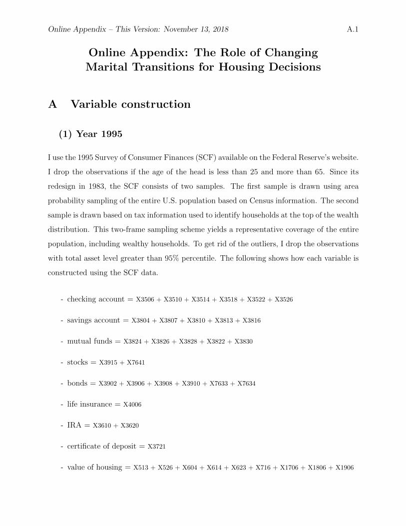
Online Appendix – This Version: November 13, 2018 A.1
Online Appendix: The Role of Changing
Marital Transitions for Housing Decisions
A Variable construction
(1) Year 1995
I use the 1995 Survey of Consumer Finances (SCF) available on the Federal Reserve’s website.
I drop the observations if the age of the head is less than 25 and more than 65. Since its
redesign in 1983, the SCF consists of two samples. The first sample is drawn using area
probability sampling of the entire U.S. population based on Census information. The second
sample is drawn based on tax information used to identify households at the top of the wealth
distribution. This two-frame sampling scheme yields a representative coverage of the entire
population, including wealthy households. To get rid of the outliers, I drop the observations
with total asset level greater than 95% percentile. The following shows how each variable is
constructed using the SCF data.
- checking account = X3506 + X3510 + X3514 + X3518 + X3522 + X3526
- savings account = X3804 + X3807 + X3810 + X3813 + X3816
- mutual funds = X3824 + X3826 + X3828 + X3822 + X3830
- stocks = X3915 + X7641
- bonds = X3902 + X3906 + X3908 + X3910 + X7633 + X7634
- life insurance = X4006
- IRA = X3610 + X3620
- certificate of deposit = X3721
- value of housing = X513 + X526 + X604 + X614 + X623 + X716 + X1706 + X1806 + X1906
Online Appendix – This Version: November 13, 2018 A.2
- mortgages and HELOCs = X1715 + X1815 + X1915 + X805 + X905 + X1005 + X1044 +
X1108 + X1119 + X1130 + X1136
- net value of housing = value of housing - mortgages and HELOCs
- total asset = checking account + savings account + mutual funds + stocks + bonds
+ life insurance + IRA + certificate of deposit + net value of housing
- homeownership dummy = 1 if value of housing > 0
- housing asset share =
net value of housing/total asset if total asset > 0
0 if total asset = 0
The variables for the years 2007, 2010, 2013 are all constructed in an analogous manner,
hence an explanation is omitted.
(2) Year 1970
(2-1) Survey of Consumer Finances (SCF)
I use the 1970 Survey of Consumer Finances (SCF) that was conducted by the Economic Be-
havior Program of the Survey Research Center at the University of Michigan. The raw data
can be downloaded from the Inter-University Consortium for Political and Social Research
(ICPSR), at the Institute for Social Research in Ann Arbor. The historical survey contains
the variables that are used to construct housing asset share and home ownership rate. It
also includes demographic information including age, sex, marital status, and educational
attainment. The historical SCF sample before 1983 is not supplemented by the second sam-
ple, so wealthy households are likely to be under-represented. Similar to the re-weighting
procedure described in Kuhn et al. (2017), I identify the observations belonging to the top
5% of the total asset distribution. Then I increase the survey weights for these households
so that 2% of wealthy households are added to the original sample. The remaining weights
are adjusted. Once this is done, I drop the observations with a total asset level greater than

Online Appendix – This Version: November 13, 2018 A.3
95% percentile under the new weights. The following shows how each variable is constructed
with this data.
- checking account = V334
- savings account = V333
- mutual funds = V335
- stocks = V336
- bonds = V337 + V338
- life insurance = V275
- certificate of deposit = V332
- net value of housing = V150 + V339 - V340
- total asset25, homeownership dummy, housing asset share are analogously defined as
with the 1995 SCF.
(2-2) Panel Study of Income Dynamics (PSID)
The Panel Study of Income Dynamics (PSID) data is the longitudinal household survey.
The 1970 PSID data does not provide a detailed breakdown of households’ portfolios into
different assets. However, the net value of housing can be constructed as V1122-V1124 and a
homeownership dummy can be set to 1 if V1122> 0. Non-housing asset is required in order
to construct housing asset share variable. To do so, I use the cross-imputation strategy as
described in section 2.2. Table 10 shows the summary statistics from the data sets in 1970
and 1995.
25There is no IRA variable for 1970. Traditional IRA was introduced with the Employee RetirementIncome Security Act of 1974 (ERISA) and made popular with the Economic Recovery Tax Act of 1981.

Online Appendix – This Version: November 13, 2018 A.4
Panel A. Mean of Variables (1970 v. 1995)
Year 1970 Year 1995Variables PSID SCF SCF
Marriage rate 0.75 0.78 0.55Age of head 43.82 43.88 42.61
Age of spouse 39.9 40.36 40.64Education of head 4.26 4.24 4.41
Housing asset share 0.54∗ 0.54 0.49Homeownership rate 0.67 0.66 0.66
Employment rate (head:M) 0.94 0.9 0.84Employment rate (head:S) 0.69 0.67 0.72
Employment rate (spouse:M) 0.52 0.51 0.66Weekly hours worked (head:M) 43.31 43.67 40Weekly hours worked (head:S) 27.89 29.44 32.13
Weekly hours worked (spouse:M) 17.68 8.47 25.69Number of observations 3267 1764 2408
Panel B. Moments of housing asset share (imputed v. raw)
Housing asset share (Year 1970) PSID SCFMean 0.54∗ 0.54
Median 0.73∗ 0.71Standard Deviation 0.44∗ 0.41
Table 10: Summary Statistics (1970 vs. 1995)
Notes: M stands for married and S stands for single. Education of head is a categorical variable (1:0-5 grades, 2: 6-8 grades, 3: 9-11 grades, 4: 12 grade/ complete high school, 5: complete college,6: post graduate studies). The value with asterisk(∗) is obtained from cross-imputation similar toBlundell et al. (2005).

Online Appendix – This Version: November 13, 2018 A.5
Vari
ab
les
Coeffi
cien
ts(S
.E.)
p-v
alu
eC
oeffi
cien
ts(S
.E.)
p-v
alu
eC
oeffi
cien
ts(S
.E.)
p-v
alu
eC
oeffi
cien
ts(S
.E.)
p-v
alu
e
log(n
on
-hou
sin
gass
et)
0.1
31∗∗∗
0.0
00
0.1
32∗∗∗
0.0
00
0.1
32∗∗∗
0.0
00
0.1
33∗∗∗
0.0
00
(0.0
15)
(0.0
15)
(0.0
15)
(0.0
15)
age
0.0
23∗∗∗
0.0
00
0.0
23∗∗∗
0.0
00
0.0
23∗∗∗
0.0
00
0.0
23∗∗∗
0.0
00
(0.0
03)
(0.0
03)
(0.0
03)
(0.0
03)
edu
cati
on
0.0
68∗∗∗
0.0
00
0.0
68∗∗∗
0.0
00
0.0
68∗∗∗
0.0
00
0.0
68∗∗∗
0.0
00
(0.0
15)
(0.0
15)
(0.0
15)
(0.0
15)
marr
iage
du
mm
y0.1
92∗∗∗
0.0
04
0.1
85∗∗∗
0.0
08
0.1
92∗∗∗
0.0
04
0.1
85∗∗∗
0.0
07
(0.0
67)
(0.0
69)
(0.0
67)
(0.0
69)
wee
kly
hou
rsw
ork
ed0.0
03∗
0.0
98
0.0
03
0.1
04
0.0
04∗
0.0
81
0.0
04∗
0.0
84
(0.0
02)
(0.0
02)
(0.0
02)
(0.0
02)
hom
eow
ner
ship
du
mm
y3.8
35∗∗∗
0.0
00
3.8
32∗∗∗
0.0
00
3.8
37∗∗∗
0.0
00
3.8
34∗∗∗
0.0
00
(0.0
59)
(0.0
59)
(0.0
59)
(0.0
60)
chil
dre
nd
um
my
——
0.0
24
0.6
90
——
0.0
25
0.6
84
(0.0
61)
(0.0
61)
emp
loym
ent
du
mm
y—
——
—-0
.075
0.4
64
-0.0
75
0.4
62
(0.1
03)
(0.1
03)
con
stant
-3.0
98∗∗∗
0.0
00
-3.1
24∗∗∗
0.0
00
-3.0
67∗∗∗
0.0
00
-3.0
94∗∗∗
0.0
00
(0.1
77)
(0.1
89)
(0.1
82)
(0.1
94)
nu
mb
erof
ob
serv
ati
on
s1570
1570
1570
1570
Ad
just
edR
-squ
are
d0.7
94
0.7
94
0.7
94
0.7
94
Tab
le11
:O
LS
Reg
ress
ion
Res
ult
s(S
CF
1970
)
Notes:
Sta
tist
ical
sign
ifica
nce
isex
pre
ssed
wit
h∗∗∗ :<
0.01
,∗∗
:<
0.05
,∗ :<
0.1

Online Appendix – This Version: November 13, 2018 A.6
B Posterior draws
Figure 19: Histogram of Posterior Draws
Figure 20: Cumulative Mean of Posterior Draws