Lawre

nce

Liverm

ore

National

Labora

tory

UCRL-ID-126085

A High Shear Stress Segment along the San Andreas Fault: Inferences Based on Near-Field Stress Direction and Stress

Magnitude Observations in the Carrizo Plain Area

David A. CastilloLeland W. Younker

January 30, 1997

This is an informal report intended primarily for internal or limited external distribution. The opinions and conclusions stated are those of the author and may or may not be those of the Laboratory.Work performed under the auspices of the U.S. Department of Energy by the Lawrence Livermore National Laboratory under Contract W-7405-ENG-48.

DISCLAIMER

This document was prepared as an account of work sponsored by an agency of the United States Government. Neitherthe United States Government nor the University of California nor any of their employees, makes any warranty, expressor implied, or assumes any legal liability or responsibility for the accuracy, completeness, or usefulness of anyinformation, apparatus, product, or process disclosed, or represents that its use would not infringe privately ownedrights. Reference herein to any specific commercial product, process, or service by trade name, trademark,manufacturer, or otherwise, does not necessarily constitute or imply its endorsement, recommendation, or favoring bythe United States Government or the University of California. The views and opinions of authors expressed herein donot necessarily state or reflect those of the United States Government or the University of California, and shall not beused for advertising or product endorsement purposes.

This report has been reproduceddirectly from the best available copy.

Available to DOE and DOE contractors from theOffice of Scientific and Technical Information

P.O. Box 62, Oak Ridge, TN 37831Prices available from (615) 576-8401, FTS 626-8401

Available to the public from theNational Technical Information Service

U.S. Department of Commerce5285 Port Royal Rd.,

Springfield, VA 22161

1

A High Shear Stress Segment along the San Andreas Fault:Inferences Based on Near-Field Stress Direction

and Stress Magnitude Observations in the Carrizo Plain Area

David A. Castillo* and Leland W. Younker

Lawrence Livermore National Labortory

Livermore, California 94551

* Now at:Department of Geology and Geophysics, University of Adelaide, Adelaide, SouthAustralia, AUSTRALIA 5073Email: castillo@timor.geology.adelaide.edu.auPhone: (61-08-8303-3870)Fax: (61-08-8303-4347)

2

Abstract

Nearly 200 new in-situ determinations of stress directions and stress magnitudes near the

Carrizo plain segment of the San Andreas fault (SAF) indicate a marked change in stress state

occurring within 20 km of this principal transform plate boundary. The predominant maximum

principal stress direction (SHmax), inferred from stress-induced breakouts in about 25 industry

wells within 3-20 km of the San Andreas fault indicate a SHmax orientation that varies between

25-45° from the fault trend. Additional in-situ observations in wells located beyond 20 km of the

fault indicate a stress state consistent with previous observations of SHmax oriented at high

angles (65-85°) to SAF. These new in-situ stress observations in wells located on either side of

the fault and at depths ranging from 0.5 - 7.4 km, show a marked transition occurring at about 20

km from the SAF, where the SHmax directions changes from "fault-normal" to "fault-oblique"

compression. Estimates of the minimum principal stress (Shmin) magnitude depth-profile,

inferred from several hydraulic fracturing treatments in production fields situated within 16-25

km east of the SAF, indicate a strike-slip stress regime with Shmin/Sv ~ 0.7. Estimates of SHmax

magnitudes based on frictional faulting theory and the observed style of faulting (strike-slip and

reverse faulting), suggest that the level of shear stress on SAF-parallel planes increases towards

the fault.

A natural consequence of this stress transition at 20 km distance from the fault is that if the

observed near-field "fault-oblique" stress directions are representative of the fault stress state, the

Mohr-Coulomb shear stresses resolved on San Andreas sub-parallel planes is substantially

greater than previously inferred based on fault-normal compression. Although the directional

stress data and near-hydrostatic pore pressures, which exist within 15 km of the fault, supports a

high shear stress environment near the fault, appealing to elevated pore pressures in the fault

zone (Byerlee-Rice Model) merely enhances the likelihood of shear failure.

These near-field stress observations within 20 km of the San Andreas fault raises important

questions regarding what previous stress observations have actually been measuring. The "fault-

normal" stress direction measured out to 70 km from the fault can be interpreted as representing

a comparable depth average shear strength of the principal plate boundary. Stress measurements

closer to the fault reflects a shallower depth-average representation of the fault zone shear

strength. If this is true, only stress observations at fault distances comparable to the seismogenic

depth, will be representative of the fault zone shear strength. This is consistent with results from

dislocation modeling where there is a pronounced shear stress accumulation out to 20 km of the

fault as a result of aseismic slip within the lower crust loading the upper locked section. Beyond

about 20 km, the shear stress resolved on San Andreas fault-parallel planes becomes negligible.

3

Introduction

Over the past 30 years, much has been learned about the kinematics of transform fault

motion, in particular, from work conducted along the San Andreas fault in California. Although

recent advances in seismological, geodetic, and wellbore measurements have greatly improved

our understanding of this major plate boundary, there remains several unresolved issues.

Probably the most paramount of these issues is what has been called within the scientific

community as the San Andreas stress/heat-flow paradox. Laboratory simulations of frictional

faulting would suggest a "strong" San Andreas fault with shear stresses, averaged over

seismogenic depths (upper 20 km) ranging from 50-100 MPa (e.g., Byerlee, 1978; Sibson, 1973,

1983; Brace and Kohlstedt, 1980). The shear stresses implied by a "weak" San Andreas would

be on the order of the earthquake stress drops, or less than 20 MPa (e.g., Lachenbruch and Sass,

1980). The lack of a appreciable long-term frictional heat-flow anomaly along the SAF would

be consistent with a "weak" fault (Brune et al, 1969; Henyey and Wasserberg, 1971;

Lachenbruch and Sass, 1973, 1980).

Within the past decade, in-situ data collected adjacent to the San Andreas supports the

concept of a "weak" fault, based on the analysis of earthquake focal mechanisms and stress-

induced wellbore breakouts indicating that the maximum horizontal principal stress (SHmax) is at

high angles (about 65-85°) to the San Andreas (Zoback et al., 1987; Mount and Suppe, 1987;

Jones, 1988; Oppenheimer et al., 1988 ). A majority of these observations come from either well

data in the Central Valley but beyond 20 km or so from the San Andreas, although, a few of the

earthquake focal mechanism solutions are from the fault zone itself (Zoback and Beroza, 1993).

That fault-parallel fold axes ocurr along the western margin of the Central Valley, implies that

this "fault normal" SHmax orientation exist within 20 km of the fault despite the lack of reliable

well data (Zoback et al., 1987; Mount and Suppe, 1987). Nonetheless, the lack of a frictional

heat-flow anomaly, a regional "fault-normal" SHmax orientation, and fault-parallel fold axes

points to the hypothesis that the San Andreas fault is a "weak" plate boundary.

The heat-flow and directional stress constraints along the SAF can be satisfied by a marked

decrease in the coefficient of friction of the fault gouge materials from µ=0.6-0.8 (Byerlee, 1978)

to µ<0.2. Moore et al., (1996) has recently demonstrated that the serpentinite mineral chrysotile,

originally thought to have explained the relative weaknesses inherit in fault gouge materials,

approaches coefficients of friction typical of Byerlee's results at relatively high confining

stresses. Therefore, a marked reduction in the coefficient of friction reduction is insufficient to

explain the low shear stresses inferred from the in-situ data (heat-flow and stress directions).

Elevating the in-situ pore pressure would reduce the effective normal stress, however, high

fluid pressures cannot exceed the least principal stress once the angle between SHmax and the

fault exceds ~60° (Scholz, 1989; Lachenbruch and McGarr, 1990). Large-scale yielding could

4

lead to an increase in the magnitudes of the principal stresses within the fault zone relative to

values immediately outside the fault (e.g., Byerlee, 1990; Rice, 1992). This increase in stress

magnitudes could support an elevation in pore pressure, and thereby, rotate the stress field within

the fault zone.

120  119 

120  119 

35°  35 

120° 119° 30' 119° 

120°  119° 30' 119° 

35° 30'

35° 

35° 30'

Plain

Carrizo

San Andreas Fault

S. SierraNevada

Mtns

Bakersfield

Taft

SodaLake

Calienta Range

Wheeler Ridge F.

Pleito Thrust F.

San Juan F.

S. Cuyama F.

Morales Thrust F.

Southern San Joaquin Valley

White

Wolf F

SAF

1857 Tejon Earthquake

Figure 1. Location map of the San Andreas fault along the Carrizo Plain segment in central California.Bold fault lines correspond to faults that have ruptured in historic time, such as the 1857 ~M8 Tejonearthquake along the San Andreas fault and the 1952 M7.8 Kern County earthquake along the WhiteWolf fault. Other faults delineate rupture in Quaternary time. Dashed line correspond to fold axes ofPliocene age or younger.

Several dynamic mechanisms have been proposed that might explain the low strength of the

SAF appealing to processes associated directly with the propagation of seismic rupture. These

processes range from transient high fluid pore pressure (Lachenbruch, 1980), dilational wave-

induced reductions in normal stress (Brune, 1993), and fluidization of fault zone material due to

channeling of acoustic waves (Melosh, 1979, 1996).

Despite the recent surge in proposed explanations for a "weak" SAF, the physical

mechanism(s) governing the strength of the SAF are far from being clearly understood. For

instance, we have no direct in-situ evidence at seismogenic depths that can be used to evaluate

fault zone dynamics in terms of structure, stress, fluids, and chemical processes. To begin

addressing these discrepancies, a joint effort between LLNL, U.S. Geological Survey, and

Stanford University has been gaining momentum design to drill a 10 km deep hole into the San

5

Andreas fault, penetrating the fault at several depths. This report reflects an intiative undertaken

at LLNL to characterize the stress state along key segments of the fault for drill site selection.

This is particularly important since it will be of paramount importance that data collected during

deep drilling into the SAF be interpreted in context of the surrounding crust.

In this study, we have collected an abundance of in-situ stress directions and stress

magnitudes from the petroleum industry, especially within 20 km of the fault. This has given us

an unprecedented opportunity to examine the near-field stress state to within 3 km of the SAF. A

equally important intiative, pioneered by LLNL has been to create new tools and technologies

necessary to drill and collect critical data in the harsh physical environments expected at these

drilling depths.

Background

The Carrizo Plain segment of the San Andreas fault proper is the simplest and easily

recognized segment of this major plate boundary. In the Carrizo plain region, the SAF divides a

8km+ sequence of marine sediments of the southern San Joaquin Valley to the northeast, from a

sequence of non-marine sediments and crystalline rocks of the Salinian Terrane to the southwest

(Graham and Olsen, 1988). The well-delineated and narrow (~few kilometers) trace of the SAF

within the northern limits of the Carrizo Plain, develops into a series of pressure ridges further

south as the SAF progressively turn eastward (Figure 1). Offset stream drainage and other

geomorphic features provides quantitative evidence of strike-slip motion along this major plate

boundary (Lawson et al., 1908; Wallace, 1968; Sieh and Jahns, 1984; Grant and Sieh, 1994;

Grant and Donnellan, 1994). The SAF last ruptured in this regions in the Great 1857 M=7.8

Fotrt Tejon earthquake (Ellsworth, 1990) along a total length of about 300 km with as much as 9-

11 m of slip along the Carrizo plain segment (Grant and Donnellan, 1994). The lack of current

seismicity and paleoseismic studies suggest that the Carrizo plain segment ruptures only during

great earthquakes (Sims, 1993 ). The accumulated transform slip over the past 15-20 Ma, when

motion initiated in the Carrizo plain, has been about 315 km (Graham et al, 1989; Sims, 1993).

The average slip rate up to about 5 Ma is about 10 mm/yr, increasing to a present-day slip rate of

about 33 mm/yr based on paleoseismic and geodetic evidence (Sieh and Jahns, 1984; Eberhart-

Phillips et al., 1990; Lisowski et al., 1991; Grant and Sieh, 1993; Grant and Donnellan, 1994).

The stress maps in Central California prior to this study presented striking evidence that the

San Andreas may be a "weak" plate boundary (Zoback et al., 1987; Mount and Suppe, 1987).

Observations of wellbore breakouts and earthquake focal mechanisms ranging in distance from a

few kilometers to ~ 70 km from the fault, and along a distance that nearly stretches its entire

length, have long been regarded as representative of the stress state resolved on the San Andreas.

Although there were few in-situ measurements within 20 km of the fault, particularly in Central

6

California, evidence supporting the notion that this fault-normal stress state extended up to the

fault were the SAF-parallel fold axes (Figure stress).

Near-Field In-Situ Stress Data

Data from over 300 wells have been analyzed for stress-induced wellbore breakouts and pore

pressure estimates adjacent to the Carrizo plain segment of the San Andreas fault (SAF). A

majority of the wells are located northeast of the SAF in the San Joaquin basin, although several

critical wells are situated in the Carrizo plain area southwest of the fault. Depths over which

reliable data were obtained ranges from about 0.5 - 7.4 km deep, with the most reliable stress

indicators generally restricted to 1 km or deeper. Estimates of the stress orientation ranged from

3- 65 km from the San Andreas fault in wells located primarily in active hydrocarbon production

fields. Without exception, wells located within 15 km of the San Andreas were drilled as

hydrocarbon exploration 'wildcat' wells.

020406080

100120

3000

3200

3400

3600

3800

4000

Arco CREE FEE 1-A

(5.4 km NE of SAF)

030

60

90

120

150180

210

240

330

Cum

ulat

ive

Bre

akou

t L

engt

h (m

)

-40 0 40 80 120SHmax (Deg)

Cen

ter

Dep

th (

met

ers)

c)

d)

a)

b)

Carrizo Plain 1-16

( 3.2 km SW of SAF )

-40 0 40 80 120

0

500

1000

1500

2000

2500

SHmax (Deg)

Cen

ter

Dep

th (

met

ers)

0

20

40

60

80

1000

30

60

90

120

150180

210

240

330

Cum

ulat

ive

Bre

akou

t L

engt

h (m

)

Figure 2. SHmax stress directions for selected wells in the Carrizo Plain area. Top plot for each well showsSHmax directions versus depth inferred from wellbore breakouts with horizontal error-barscorresponding to directional uncertainties. Vertical bars for each point illustrates the Vertcal extentalong which the breakout was observed. The bottom plot for each well represents the length-weightedSHmax directions for data in that specfic well. a) and b) Carrizo Plain 1-16; c) and d) Arco Cree Fee 1-A; e) and f) Tenneco TWI Fee 1-33; g) and h) Grayson Owen 1-35; i) and j) UO-NPR 385-12Z; k) andl) UO-NPR 934-29R.

7

0

50

100

150

2000

30

60

90

120

150180

210

240

330

Cum

ulat

ive

Bre

akou

t L

engt

h (m

)

-40 0 40 80 120

1000

1500

2000

2500

3000

3500

Grayson Owen 1-35

(13.5 km SW of SAF)

SHmax (Deg)

Cen

ter

Dep

th (

met

ers)

g)

h)

Tenneco TWI Fee 1-33

( 7 km SW of SAF )

-40 0 40 80 120

1200

1000

1400

1600

1800

2000

SHmax (Deg)

Cen

ter

Dep

th (

met

ers)

e)

020406080

100120140

030

60

90

120

150180

210

240

330

Cum

ulat

ive

Bre

akou

t L

engt

h (m

)

f)

050

100150200250300350

-40 0 40 80 120

1000

0

2000

4000

5000

3000

7000

6000

8000

SHmax (Deg)

Cen

ter

Dep

th (

met

ers)

030

60

90

120

150180

210

240

330

Cum

ulat

ive

Bre

akou

t L

engt

h (m

)

UO-NPR 934-29R

( 20.8 km NE of SAF )

k)

l)

0

20

40

60

80

100

-40 0 40 80 120

1600

1800

2000

2200

2400

2800

2600

3000

SHmax (Deg)

Cen

ter

Dep

th (

met

ers)

030

60

90

120

150180

210

240

330

Cum

ulat

ive

Bre

akou

t L

engt

h (m

)

UO-NPR 385-12Z

( 22.5 km NE of SAF )

i)

j)

Figure 2. Continued

8

A catalog of SHmax directions inferred from stress-induced wellbore breakouts is the primary

contribution in this manuscript. Two hundred of the 300 or so wells used in this study indicated

reliable wellbore breakout directions, which in theory, are aligned perpendicular to the maximum

principal horizontal stress (SHmax). The cummulative length of breakout intervals observed for

the entire study was in excess of 15,000 meters, with representative examples of average

directions for selected wells shown in Figures 2a-2l. Only stress data for a particular wells

where the total variability was less than 25° are shown in these figures. For comparison, data of

quality A and B from the World Stress Data Base (Zoback and Zoback, 1991) are also shown.

35 °

120 ° 119 °

(> 1km Deep)

San Andreas fault

20 km

Carrizo PlainElk Hills NPR

a)

T 1-20

CP 1-16

T 1-33

ACF 1-A

GO 1-35

NPR 385NPR 934

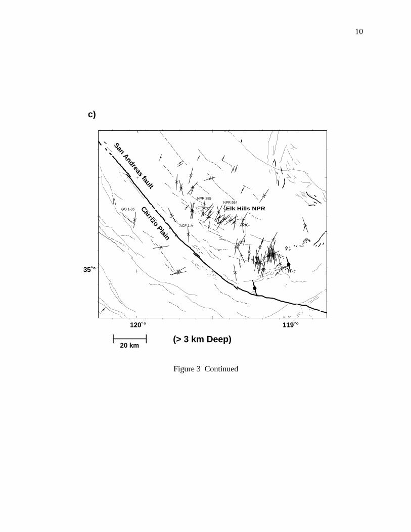
Figure 3 Maps showing the maximum principal stress orientations (SHmax) along the San Andreas faultand surrounding regions at different observation depths. Inward facing arrows are stress indicatorsinferred from wellbore breakouts while the circled symbols are stress indicators inferred from focalmechanism inversions. a) Stress directions using data 1 km and deeper. b) Stress directions usingdata 2 km and deeper. c) Stress directions using data 3 km and deeper. Stress observations situated20 km or more from the San Andreas fault suggest that the fault has little shear stress resolved on it,while data within 20 km, showing stress directions that are 30-45° from the fault and in some cases asclose as 3 km, suggest relatively high levels of shear stress resolved on the fault. CP 1-16, CarrizoPlain 1-16; T 1-20, Tenneco 1-20; T 1-33, Tenneco TWI Fee 1-33; GO 1-35, Grayson Owen 1-35;ACF 1-A, Arco CREE Fee 1-A; NPR 385, UO-NPR 385-12Z; NPR 934, UO-NPR 934-29R

9

35 °

120 ° 119 °

(> 2 km Deep)

San Andreas fault

20 km

Carrizo Plain

Elk Hills NPR

b)

T 1-20

CP 1-16

T 1-33

ACF 1-A

GO 1-35

NPR 385NPR 934

Figure 3 Continued

10

35 °

120 ° 119 °

(> 3 km Deep)

San Andreas fault

20 km

Carrizo Plain

Elk Hills NPR

c)

ACF 1-A

GO 1-35

NPR 385NPR 934

Figure 3 Continued

11

Examples of SHmax stress directions inferred from wellbore breakouts in 5 wells are shown

in Figures 2a-2l. These wells are located between 5.4 and 22.5 km from the San Andreas fault

with observations ranging from 0.5 - 7.4 km deep. The deepest stress observation at 7.4 km

depth was measured in well UO-NPR 934-29R situated about 21 km northeast of the San

Andreas (Figures 2k and 2l) indicating a dominant northeast-southwest SHmax stress direction,

consistent with previous observations (Zoback, et al., 1987; Mount and Suppe, 1987). However,

wells located closer to the San Andreas fault display a markedly different SHmax direction. The

average SHmax direction seen in Carrizo 1-16 and Arco Cree Fee 1-A (Figure 3), located within

5.4 km of the San Andreas fault, indicates a well-pronounced north-south orientation at a depth

of about 2.5 and 4 km, respectively. Examples of shallower stress measurements in Tenneco

TWI Fee 1-33 (~ 1.9 km deep) and Grayson Owen 1-35 (~ 3.1 km deep), located 7 and 13.5 km

southwest of the San Andreas fault, respectively, also indicate a consistent north-south SHmax

direction (Figures 2d-2e).

The small-scale variations in the stress versus depth plots (Figures 2a-2l) are indicators of

local perturbations in the stress field where the wellbore has possibly intersected faults and/or

fractures. In cases where computed dip-meter logs were available in the intervals of these local

stress perturbations, there were pronounced structural discontinuities that may be due to faulting.

Examples of these small scale and local stress variations have been observed elsewhere in the

San Joaquin basin (Castillo and Zoback, 1994) and in other stress provinces (Barton and Zoback,

1994).

Non-uniform stress field

The non-uniformity in the stress state adjacent to the Carrizo plain segment of the San

Andreas fault is best illustrated in map view and as plots showing stress directions versus

distance from the San Andreas (Figures 3, 4, and 5). We've chosen to show the average stress

direction for each well in terms of observation depths. For instance, Figure 3a is a map showing

stress directions from observations 1 km or deeper. Figures 3b and 3c correspond to average

stress directions from those wells with observations deeper than 2 km and 3 km, respectively. In

many cases where breakouts were observed over depths of several kilometers, the same average

stress direction will appear on subsequent maps showing deeper data. Aside from the small-

scale stress variations seen in a few of the wells (Figure 3) there were no large scale changes in

the stress field in any particular well that would suggest systematic and depth dependent

rotations in the stress field. To avoid stress complications related to the 'big bend' segment of the

San Andreas fault, our discussions will be restricted to those data on either side of the linear

Carrizo plain segment before the fault enters into the "big bend" area (Figures 1 and 3). .

12

In most of the wells situated beyond ~ 20 km from the San Andreas fault, the dominant

SHmax stress direction is consistent with previous observations of 'fault-normal' compression

(Zoback et. al., 1987; Mount and Suppe, 1987, Castillo and Zoback, 1994). This remains the

case even after the shallower data, some of which shows locally conflicting stress directions, is

filtered out showing only stress observations deeper than 3 km (Figure 3c). This is most

pronounced within the eastern portions of the Elk Hills Naval Petroleum Reserve (NPR) fields

where the largest concentration of data was analyzed. Overall, these 'fault-normal' stress

directions are geologically consistent with the compressional fold axes in the central valley

which are shown as dashed lines in Figures 3a-c.

An important pattern that emerges considering the stress data within 20 km or so is that the

SHmax direction shows a pronounced rotation from northeast-southwest compression to nearly

north-south becoming oblique to the trace of the San Andreas fault (Figures 3a-c). This pattern

of 'fault-oblique' compression is observed on both sides of the fault to depths approaching 4 km.

As in the case with data located 20+km from the fault, filtering to include 2+ km deep

observations eliminates some of the inconsistent stress orientations which either show fault-

parallel compression or have a stress field that resolves left-lateral shear on San Andreas parallel

planes. The implication is that these shallower measurements may be reflecting local stress

anomalies and are likely not representative of a stress field associated with the San Andreas fault.

Interestingly, the perpendicular distance from the San Andreas fault where this stress

transition from far-field fault-normal to near-field fault-oblique compression occurs appears to

show a slight fault-strike dependence. Along the central and northwest sectors of our study area,

stresses appears to rotate at about 20 km from the fault. However, near the 'big bend' area, there

is a tendency for SHmax to remain near fault-normal up to about 10 km from the fault (Figure 3a-

c). If the fault restraining character produced by the 'big bend' region contributes to the rotation

in the stress field, one would expect the opposite variations along strike, namely, fault-oblique

compression would be seen at further distances from the fault instead of 10 km or so. Perhaps

along strike variations in fault rheology are contributing or controling the stresses (more on this

later).

Probably the most detailed evidence showing the nature of this stress transition occurs within

the Elk Hills NPR (Figure 4). In general, the Elk Hills NPR can be subdivided into two

regionally distinct structures. The eastern half is characterized by a east-west trending anticlinal

structure that changes to a more northwest-southeast orientation along the western half of the

reserve. Along with this change in structure trend comes a gradual counter-clockwise rotation in

SHmax stress directions from northeast-southwest to a more northerly direction at the western

extremes of the Elk Hills structure (Figure 4). Although there is a ~7 km gap between the

western Elk Hills NPR and the Cymric field further west, the transition from 'fault-normal' to

13

35° 15'35° 15'

119° 30' 119° 15'119° 45'

119° 30' 119° 15'119° 45'

0 5 10 15 20 km

Elk Hills Naval Petroleum Reserve-1

San Andreas Fault

NPR-1-934-29R7.4 km deep

NPR-1-385-12Z3 km deep

Carrizo Plain

Cymric Field

Arco Cree Fee 1-A

Bradfield 42-11

Figure 4 Detailed stress map within the Elk Hills Naval Petroleum Reserve spanning a distance of 15 - 30km from the San Andreas fault. Stress symbols are the same as Figure 2. Stress observations withinthis range provides an excellent opportunity to examine details of the SHmax stress transition fromNE-SW to N-S compression. Over 70 wells analyzed in the Elk Hills area indicates that the apparenttransition occurrs between 20 - 25 km from the San Andreas fault.

'fault-oblique' appears to be complete in the Cymric area since stress measurements in excess of

3 km deep show a well-pronounced north-south compression (Figure 4).

Distances beyond 20 km or so, the SHmax directions are remarkably consistent with the trend

of the fold axes which are sub-parallel to the San Andreas fault. In particular, one of the

important arguments supporting the extrapolation of this stress field up to the plate boundary was

that these fold axes remain sub-parallel to very near distances to the fault (Zoback et al., 1987;

Mount and Suppe, 1987). Emerging from these new stress observations situated within 20 km of

the fault, is an apparent inconsistency between the trend of these fold axes and the fault-oblique

stresses (Figures 3-4). If the development of the SAF-parallel folds are a consquence of SHmax

acting nearly perpendicular to the structure, one is left with explaining the ~45° discrepency

between the stresses and fold axes orientation. One possibility is that the folds orginally formed

oblique to the fault trace in a classical wrench tectonics fashion but have since rotated as a result

finite strain due to strike-slip motion on the San Andreas fault. There is some evidence in the

Temblor range area that tentativley supports this hypothesis (personal communicaiton, Don

Miller 1996, Stanford University). Alternatively, the folds may be the consequence of folding

within the hanging wall of an updip propagating blind thrust which could be responding to near

14

fault-normal compression, but at greater depths (>10 km). This depth-varying stress state at

distances less than 20 km from the fault will be revisited later.

0

10

20

30

40

50

60

70

80

90

100

0 10 20 30 40 50 60

( > 1 km deep)

Azi

mu

th w

rt f

ault

str

ike

(deg

)A

zim

uth

wrt

fau

lt s

trik

e (d

eg)

Azi

mu

th w

rt f

ault

str

ike

(deg

)

Distance from SAF (km)

Distance from SAF (km)

Distance from SAF (km)

0

10

20

30

40

50

60

70

80

90

100

0 10 20 30 40 50 60

( > 3 km deep )

0

10

20

30

40

50

60

70

80

90

100

0 10 20 30 40 50 60

( > 2 km deep)

a)

b)

c)

Figure 5 Stress versus Distance from the San Andreas fault. Azimuths are measured with respect to thestrike of the fault (~N40°W). Included are only data adjacent to the Carrizo plain segment butremoved from the 'Big Bend' area in order to eliminate any geometric complications. a) Relative faultand stress azimuth for data 1 km or deeper. b) Relative fault and stress azimuth for data 2 km ordeeper. c) Relative fault and stress azimuth for data 3 km or deeper. As was the case in Figure 2, databetween 20 km and nearly 55 km from the San Andreas fault suggest that the fault can not ustain agreat deal of shear stress. However, within 20 km or so of the fault, the relative azimuth changes from~75° to about 30-45° from the fault.

15

There are four exceptional stress anamolies that cannot be explained by shallow filtering

since they presist to depths in excess of 3 km. One set of wells are located west of the SAF

along the western margins of the Carrizo plain proper (Figure 3a-c). These three wells, situated

about 12-15 km from the fault, show nearly fault-normal compression but with a small degree of

left-lateral shear stresses on San Andreas parallel planes. That these anomalous stress directions

presist to depth in excess of 3 km suggests strong local control. Based on an east-west cross-

section that includes these wells (Davis et al., 1988), the observed stress-induced wellbore

breakouts appears to be confined to an interval located between the east-dipping Morales thrust

and White Rock thrust faults with east-west convergence beginning about 3 Ma. Between these

wells and the SAF, are two wells; Carrizo Plain 1-16 (Figure 3) and Tenneco TWI Fee 1-33

(Figures 2c, 2d and 3) that indicate a rotation to N-S compression or fault-oblique. Another

exception includes a well situated on the east side of the fault showing nearly fault-parallel

compression, which is consistent with a nearby shallow well also showing 'fault-parallel'

compression (Figure 3a). Unfortunately there are no other wells within 10 km of these wells that

would characterize how extensiveness this anomaly is in the area.

An alternate way of showing this transitional stress state is to plot stress orientations relative

to the strike of the San Andreas fault for wells on both side of the fault (Figures 5a-c). Using a

depth filtering scheme as in Figures 3a-c, this representation illustrates a depth consistent pattern

of stress rotation at a distance of ~ 20 km from the San Andreas fault. Although there is some

noise in the data, as to be expected in 4-arm caliper data, the density of well coverage strongly

suggests that dispite this apparent scatter in the data (which diminishes when only deeper data is

considered), there is a well pronounced transition from fault-normal compression in the far-field

to fault-oblique witihn ~20 km from the San Andreas fault (Figure 5a-c).

There are far too few wells to test if this pattern of fault-oblique compression is still evident

if only data in the 4+ km depth range is considered, however, Arco Cree Fee 1-A (Figures 2a-b,

3c and 4) shows a relative orientation of 33° with respect to the fault at depths in excess of 3.9

km and about 5.4 km east of the fault. Beyond 20 km from the fault, most of the data deeper

than 4 km lies between 55° and 90° relative to fault strike.

Crustal Pore Pressure

Nearly 300 wells were used to estimate crustal pore pressure adjacent to the San Andreas

fault in the Carrizo plain area with a majority of the data from the San Joaquin basin. Pore

pressure estimates were based either on mud weight records or drill stem tests. There was

agreement in those cases where both data types were used. A mud weight log is a recording of

the density of drilling mud used during the drilling process, which in principal reflects, the

formation pore pressure if there is a pressure balance between the borehole fluids and the

16

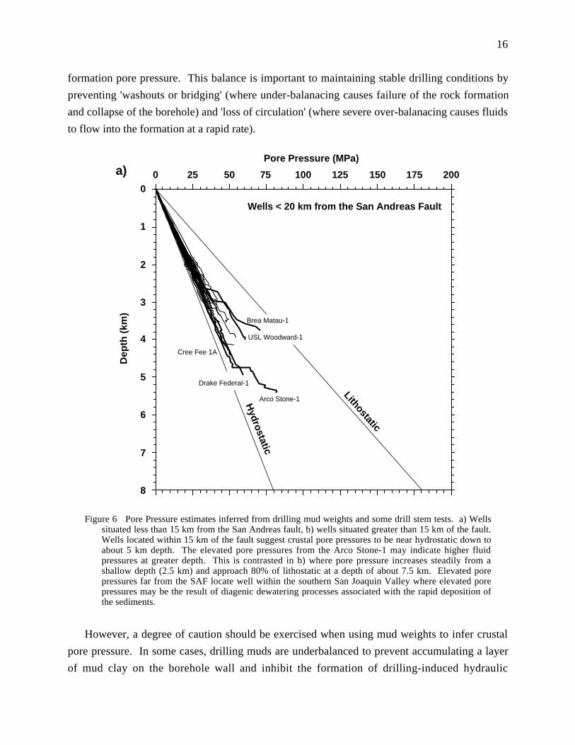
formation pore pressure. This balance is important to maintaining stable drilling conditions by

preventing 'washouts or bridging' (where under-balanacing causes failure of the rock formation

and collapse of the borehole) and 'loss of circulation' (where severe over-balanacing causes fluids

to flow into the formation at a rapid rate).

USL Woodward-1

Arco Stone-1

Cree Fee 1A

Brea Matau-1

Drake Federal-1

Lithostatic

Hydrostatic

00

1

2

3

4

5

6

7

8

25 50 75 100 125 150 175 200

Pore Pressure (MPa)

Dep

th (

km)

Wells < 20 km from the San Andreas Fault

a)

Figure 6 Pore Pressure estimates inferred from drilling mud weights and some drill stem tests. a) Wellssituated less than 15 km from the San Andreas fault, b) wells situated greater than 15 km of the fault.Wells located within 15 km of the fault suggest crustal pore pressures to be near hydrostatic down toabout 5 km depth. The elevated pore pressures from the Arco Stone-1 may indicate higher fluidpressures at greater depth. This is contrasted in b) where pore pressure increases steadily from ashallow depth (2.5 km) and approach 80% of lithostatic at a depth of about 7.5 km. Elevated porepressures far from the SAF locate well within the southern San Joaquin Valley where elevated porepressures may be the result of diagenic dewatering processes associated with the rapid deposition ofthe sediments.

However, a degree of caution should be exercised when using mud weights to infer crustal

pore pressure. In some cases, drilling muds are underbalanced to prevent accumulating a layer

of mud clay on the borehole wall and inhibit the formation of drilling-induced hydraulic

17

fractures.

18

Sand Hills64X-34

Pleito Creek86X-18

00

1

2

3

4

5

6

7

8

25 50 75 100 125 150 175 200

Pore Pressure (MPa)

Dep

th (

km)

Central regions of the San Joaquin Basin

and > 20 km from the San Andreas FaultLithostatic

Hydrostatic

Rio Viejo27X-34

b)

Figure 6 Continued

19

954-4G

00

1

2

3

4

5

6

7

8

25 50 75 100 125 150 175 200

Pore Pressure (MPa)

Dep

th (

km)

Wells within the Elk Hills NPR and

> 20 km from the San Andreas Fault

523-32S

987-25R

934-29R Lithostatic

Hydrostatic

c)

Figure 6 Continued

20

Clay on the borehole walls reduces the response of the geologic/geophysical logs. Overbalanced

wells prevents the development of wellbore breakouts, but can cause formation fluid invasion

which also reduces the log response. The preferred method would be a series of drill stem tests

which measure pore pressure within a specific interval, however, these tests are not frequently

measured and if so, are conducted across hydrocarbon targeted intervals. Nonetheless, the

abundance of wells used to map mud-weights in the Carrizo plain probably can be used as a

rough descriminator to distinguish between areas of high or low pore pressure.

Because there seems to be a marked change in SHmax directions at about 15-20 km from the

SAF, we have regionally separated crustal pore pressure plots into wells located less than 20 km

(Figure 6a) and wells greater than 20 km from the SAF (Figure 6b). For wells in the latter

category, data has been further divided to examine details within the Elk Hills NPR (Figure 6c).

In general, the data indicates near-hydrostatic pore pressure to at least 5 km depth and within

20 km of the SAF. The Arco Cree Fee 1-A, located 5.4 km northeast of the fault indicates near-

hydrostatic pore pressure to depths approaching 4.5 km. These relatively low pore pressures are

consistent with nearly all wells situated within 20 km of the fault. In contrast, the Arco Stone-1

well, the deepest well in the area, shows a significant increase in apparent pore pressure over a

short interval below 5 km. The other two wells that indicates a significant increase in apparent

pore pressure are Brea Matau-1 and USL Woodward-1, both situated south-southeast of the SAF,

near where the fault makes a bend.

The wells located >20 km from the SAF indicate a significant increase in the apparent pore

pressure, compared to wells near the fault. There is very little difference between both regions in

the upper 3 km, however, pore pressures rapidly increase to almost 60-80% of lithostatic. The

drill-stem test conducted in Tenneco Sand Hills 64X-34 well are consistent with an average

apparent pore pressure inferred from the mud weights. The gradual increase in pore pressure in

the 7.4 km deep NPR 934-29R well begins with Po/Sv ~ 0.6 at 4 km and increases to 0.8 at total

depth.

Although speculative, the mud weight inferred increase in pore pressure below 5 km depth

and within 20 km of the fault may increase further at greater depths, which would support the

high pore pressure fault model after Byerlee (1990) and Rice (1992). However, as will be shown

later, a rigorous interpreation of the Byerlee/Rice high pore pressure model would imply a 15-20

km wide San Andreas fault zone. This is probably unlikely, because the surface trace of the SAF

is well confined to a kilometer or so zone with no clear evidence of additional SAF-parallel

strike-slip faults within 20 km of the main trace. Lower pore fluid pressures are required

adjacent to the elevated fault-zone fluid pressures, however, the data indicates the opposite with

high apparent crust pore pressures beyond 20 km of the San Andreas fault.

21

Frictional Faulting Theory for Estimating Stress Magnitudes

Estimates of the principal stress magnitudes in the vicinity of the Carrizo Plain segment of

the San Andreas fault were made using Shmin magnitudes from hydrofrac treatments in the San

Joaquin Valley, and SHmax from Frictional Faulting theory using Byerlee's law (Byerlee, 1979)

and a Mohr-Coulomb failure criteria (Jaeger and Cook, 1979). Estimates of the third and

vertical component of the stress tensor is presumed to be equivalent to the vertical lithostatic

load (i e., Sv).

Minimum Principal Stress Magnitudes (Shmin)

Hydraulic fracturing treatments in the Cymric Deep Gas Field situated about 18 km from the

SAF and the Elk Hill NPR provided reasonably consistent Shmin magnitudes to depth

approaching 3 km. The exploration wells drilled close (< 10 km) to the San Andreas fault are

normally abandoned when the well fails to produce any signs of hydrocarbons. Therefore, none

of the near-field wells have any information regarding stress magnitudes from hydraulic

fracturing treatments, since such treatments are generally used during enhanced oil recovery

efforts.

Four hydraulic fracturing treatments from the Cymric field were utilized in this study. The

relatively close spacing between wells and the consistency between estimates of Shmin

magnitudes (Figure 7a) in this area compared to other well sites in the San Joaquin Valley

suggest that Shmin this field may be representative of the stress state, at least within 18 km of the

SAF. Without additional stress information close to the fault, we will assume that the trend in

Shmin magnitudes observed in Cymric field may be representative of the stress state close to the

fault.

The relative stress magnitudes in the Cymric field, as in many other wells in the San Joaquin

Valley, are such that Shmin < Sv. The average Shmin/Sv "frac" ratio shown in Figure 7a is about

0.65, which is also consistent with other observations throughout the San Joaquin Valley, at least

below 2 km (Personal Communications, Bill Minner, Pinnacle Technologies Inc.). The possible

stress states consistent with the observed Shmin/Sv ratio are either strike-slip or normal faulting

stress regimes. Based on the observed strike-slip and reverse faulting seen within the San

Andreas fault system and within the adjacent crust, we can rule out the possibility of a normal

faulting stress regime Another reason why a normal faulting stress state can be discounted is that

the stress concentrations resulting from such a stress state could not support the development of

wellbore breakouts that are so pervasive throughout the Central Valley.

There are anomalous areas in the San Joaquin Valley where the frac ratio Shmin/Sv

approaches unity, but these place are restricted to shallow depths (< 500 m) in the diatomite

rocks within the Lost Hills and Belridge fields (Wright et al., 1996). In these situations, tiltmeter

22

arrays deployed during hydraulic fracturing treatments detect near-horizontal hydofracs

propagating away from the wellbore. Deployment of these tiltmeter arrays for deeper fracs (>

2km) in other parts of the Central Valley indicate a near-vertical hydraulic fracture implying that

the minimum principal stress is approximately horizontal.

0 10 20 30 40 50 60 70 80 90 100

0

500

1000

1500

2000

2500

3000

3500

Stress (MPa)

Dep

th (

km)

Shmin (Closure Stress)

SHmax (Frictional Faulting

Constraints, µ=0.75)

Vertical Stress (SV = pgh)

a)

Figure 7 Possible strike-slip stress state within 15 km of the San Andreas fault along the Carrizo Plainsegment. Stress states correspond to a depth of 3 km which is about the average observation depth ofwellbore breakouts showing a consistent rotation from NE-SW to N-S near the fault. a) Estimates ofthe minimum principal stress magnitude (Shmin) inferred from hydraulic fracturing treatments in theCymric field located 18 km east of the San Andreas fault, b) The inferred stress profiles rely on theassumption that hydraulic fracture gradients observed in the Cymric wells located near (~ 18 km) theSan Andreas fault are representative of the Shmin gradient. The vertical load, Sv, is based on an

average rock density of 2300 kg/m3. Possible SHmax values range from φ = 1.0 (SHmax =Sv) to alimiting factor of φ =0.38, assuming frictional faulting contraints and a coefficient of friction of µ = 0.6(Jeager and Cook, 1979). c) Equivalent 2-D Mohr Circles to the stress states shown in b) butextrapolated to a depth of 15 km.

Maximum Principal Stress Magnitudes (SHmax)

Probably the single most difficult component of the stress tensor to quantify is the maximum

horizontal stress (SHmax). Where a Shmin is well constrained using several pressure cycles of a

hydraulic fracture treatment or 'extended leakoff tests', SHmax can be estimated assuming that

subsequent pressure cycles have already exceeded the tensile strength of the rock formation and

the fracture has propagated several borehole radii away. Without, this information, we will

appeal to an alternative method for constraining SHmax utilizing the observed style of wellbore

failure. Given we can estimate a Shmin profile from the data collected in the Cymric field and

elsewhere in the Central Valley, we explore a range of possible SHmax values using a Mohr-

23

0 100 200 300 400 5000

5

10

15

Strike-Slip Stress Regime within

10-20 km of the San Andreas Fault

= Sv

SH SHSh

Stress (MPa)

Dep

th (

km)

MaximumShear .7 .5 0.38φ = 1.0

b)

-40

-30

-20

-10

0

10

20

30

40

10 80

Sh

ear

Str

ess

(MP

a)

Effective Normal Stress (MPa)

SvSh

φ=.38φ=.5φ=.7φ=1

Frictional Limit

c)

HFC

Figure 7 Continued

Coulomb failure criteria (Jaeger and Cook, 1979) which places constraints on the ratio of

maximum and minimum effective stresses in terms of the strength of the crust.

The formulation is based on a failure criterion first proposed by Coulomb (1773) that states

that the ratio of the shear (τ) and the normal stresses (σn) applied on a particular plane at failure

is equivalent to the coefficient of friction (µ), namely;

τσn

= µ (1)

24

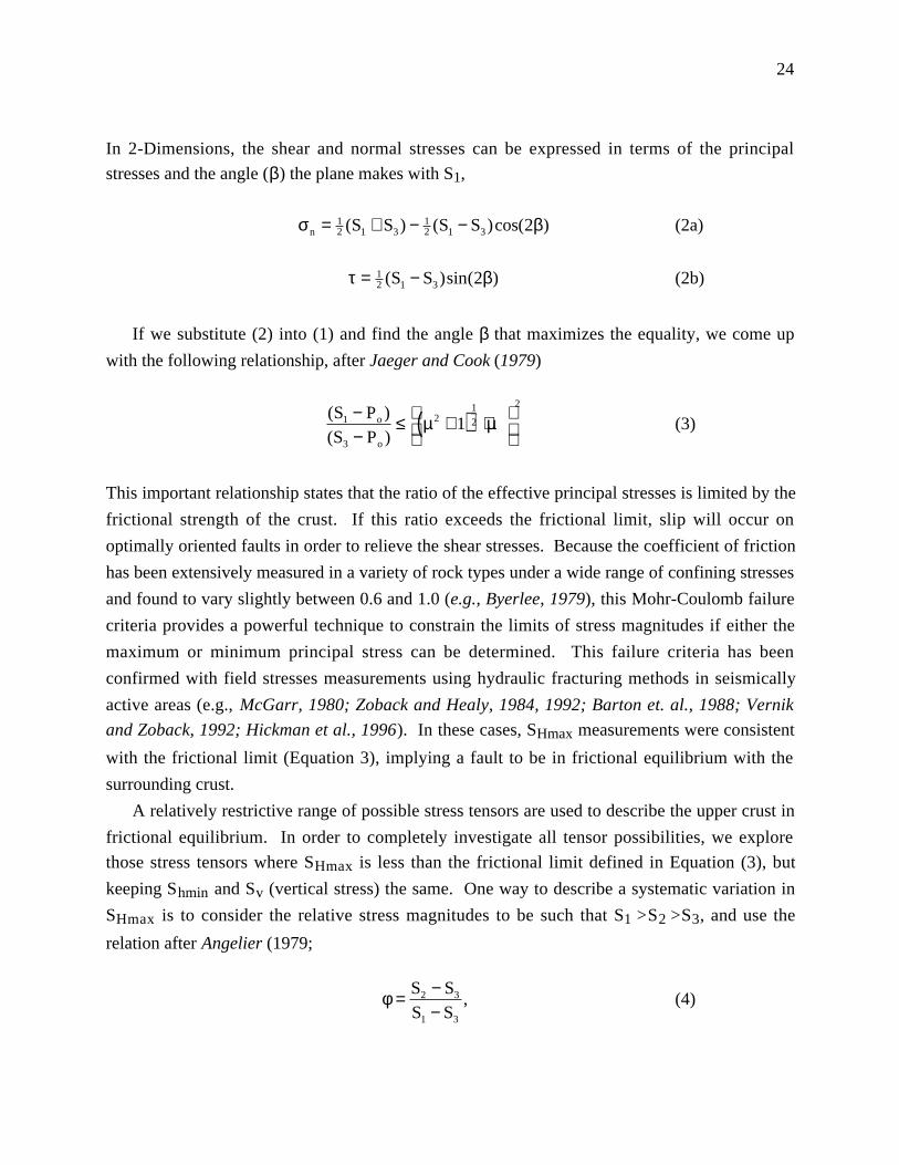
In 2-Dimensions, the shear and normal stresses can be expressed in terms of the principal

stresses and the angle (β) the plane makes with S1,

σn = 12 (S1 + S3) − 1

2 (S1 − S3)cos(2β) (2a)

τ = 12 (S1 − S3)sin(2β) (2b)

If we substitute (2) into (1) and find the angle β that maximizes the equality, we come up

with the following relationship, after Jaeger and Cook (1979)

(S1 − Po )(S3 − Po )

≤ µ2 + 1( )1

2 + µ

2

(3)

This important relationship states that the ratio of the effective principal stresses is limited by the

frictional strength of the crust. If this ratio exceeds the frictional limit, slip will occur on

optimally oriented faults in order to relieve the shear stresses. Because the coefficient of friction

has been extensively measured in a variety of rock types under a wide range of confining stresses

and found to vary slightly between 0.6 and 1.0 (e.g., Byerlee, 1979), this Mohr-Coulomb failure

criteria provides a powerful technique to constrain the limits of stress magnitudes if either the

maximum or minimum principal stress can be determined. This failure criteria has been

confirmed with field stresses measurements using hydraulic fracturing methods in seismically

active areas (e.g., McGarr, 1980; Zoback and Healy, 1984, 1992; Barton et. al., 1988; Vernik

and Zoback, 1992; Hickman et al., 1996). In these cases, SHmax measurements were consistent

with the frictional limit (Equation 3), implying a fault to be in frictional equilibrium with the

surrounding crust.

A relatively restrictive range of possible stress tensors are used to describe the upper crust in

frictional equilibrium. In order to completely investigate all tensor possibilities, we explore

those stress tensors where SHmax is less than the frictional limit defined in Equation (3), but

keeping Shmin and Sv (vertical stress) the same. One way to describe a systematic variation in

SHmax is to consider the relative stress magnitudes to be such that S1 >S2 >S3, and use the

relation after Angelier (1979;

φ = S2 − S3

S1 − S3

, (4)

25

where φ varies from 0 to 1. For a strike-slip faulting stress regime (i.e., SHmax> Sv> Shmin),

Anderson's faulting theory (Anderson, 1951) defines φ = (Sv-Shmin)/(SHmax-Shmin). When φ =0,

relative stress magnitudes are such that Sv = Shmin, or a transitional stress state that can support

both strike-slip and reverse faulting. When φ =1, stress magnitudes are such that Sv =SHmax

which is also a transitional stress state but between strike-slip and normal faulting. An example

of these possible stress states are shown in Figure 7b-c.

Upper limits for SHmax magnitudes were derived assuming frictional faulting theory, a

coefficient of friction, µ=0.75, and near-hydrostatic pore pressure. This upper limit was

determined at a depth of 3 km, corresponding to the average depth of wellbore breakouts

analyzed in this study. If we use an average Shmin value, as seen in the Cymric field, in Equation

3 to estimate the frictional limit of SHmax at hydrostatic pore pressure conditions, we find that

φ=0.4 (Equation 4). Since we do not have independent evidence to constrain SHmax values, we

cannot rule out the possibility that SHmax could be less than the frictional limit defined by

Equation 3, and as low as SHmax =Sv (φ=1). The relative stress magnitudes and corresponding

shear stresses are shown in Figure 7c. For fixed values of Shmin and Sv, any decrease in SHmax

magnitudes corresponds to a decrease in shear stress (i e., a decrease in the size of the Mohr

circle (Figure 7c) Also shown in Figure 7b is the maximum shear stress that would satisfy the

heat-flow constraint (Lachenbruch and Sass, 1980).

Shear Stresses Along the Carrizo Plain Segment of the San Andreas Fault

Having detailed stress orientation data in the SAF near-field as well as the surrounding crust

(Figures 3 and 4) and plausible stress magnitude information, provides an unprecendeted

opportunity to examine how shear stresses vary along SAF-parallel planes as a function of

distance from the fault. Using Equations 2a and 2b, and the Mohr-Coulomb failure criteria

(Jaeger and Cook, 1979) shear failure could occur when,

τ − µ(σn − P0 ) > 0 , (5)

where (σn-Po) is the effective normal stress, τ is the applied shear stress, and µ is the coefficient

of friction, where we use µ=0.6 consistent with Byerlee (1979). Using the relative stress

orientation data shown in Figure 5, the Mohr-Coulomb shear failure criteria along SAF-parallel

planes were determined using estimates of stress magnitudes discussed above. The results are

also presented in Figure 8 showing variations in shear stress as a function of distance from the

fault. The vertical bars reflect the range of possible SHmax magnitudes ranging from SHmax

=frictional limit (high φ) and SHmax =Sv (φ=1). The results indicate a strong tendency for the

Mohr-Coulomb shear stresses to increase within 20 km of the fault. Considering data farther

26

than 20 km from the fault, the Mohr-Coulomb shear failure criteria is markedly negative

implying the likelihood for shear failure is very low. Although the data would appear to be noisy

in the upper 1 km or so, the propensity for shear failure increases irrespective of filtering efforts

to depth-filter the data (Figure 8 ). This increase in shear stress in the vicinity of the SAF is

more pronounced if near-lithostatic pores pressures are considered, although, appealing to these

elevated pressures are not necessary to promote failure.

(>1 km Depth)

-50

-40

-30

-20

-10

0

10

0 10 20 30 40 50 60

Sh

ear

Str

ess

(MP

a)

Distance from San Andreas fault (km)

-50

-40

-30

-20

-10

0

10

0 10 20 30 40 50 60

Sh

ear

Str

ess

(MP

a)

Distance from San Andreas fault (km)

-50

-40

-30

-20

-10

0

10

0 10 20 30 40 50 60

Sh

ear

Str

ess

(MP

a)

Distance from San Andreas fault (km)

(>3 km Depth )

(>2 km Depth)

Figure 8 Mohr-Coulomb failure criteria (shear stress) using the possible stress states at 3 km depth shownin Figure 6 and the stress direction profile data shown in Figure 3. The failure criteria as a function ofdistance from the San Andreas fault considering only data with observations a) ≥ 1 km deep, b) ≥ 2km deep, and c) ≥ 3 km deep. The vertical limits indicated by the bars represent the bounding limits ofstress states considered in Figure 6 with φ ranging from 1.0 to 0.38. The important issue is that theconditions for shear failure along SAF parallel planes (Mohr-Coulomb failure criteria > 0) markedlyincreases within 20 km of the San Andreas fault.

27

Non-Uniform Fault Strength

Probably the most profound observation that emerges from this study is that the Carrizo plain

segment of the San Andreas fault appears to sustain a relatively higher level of shear stress

compared to other neighboring segments, based on stress directions. Although our stress

magnitudes information is not as well constrained as our stress directions, the relatively high

stress differentials seen at 15+ km from the fault would have to decrease markedly near the fault

to produce a low shear stress environment along the SAF, and still satisfy the observed fault-

oblique orientations and the apparent lack of a heat-flow anomaly. This same low stress

differential produces insufficient stress concentrations around the borehole wall that could not

support the widespread development of wellbore breakouts as seen throughout the San Joaquin

Valley.

A comparison between stress direction data observed along the Carrizo plain segment and

three other segments (i.e., San Francisco Bay Area, central California between San Juan Bautista

and Parkfield, and Mojave desert) suggests that the Carrizo plain may be unique. Although the

density coverage along the three comparison segments is less than the Carrizo plain area (Figure

9), the current data along the San Francisco, Central California and Mojave segments still

suggest that these segments have low resolved shear stresses (Figure 10). The San Francisco

Bay Area is complicated because the San Andreas Fault System widens considerably from

several kilometers in Central California to 70-100 km between the Bay Area and the Mendocino

Area (e.g., Wallace, 1990; Castillo and Ellsworth, 1992). The dominant stress indicators in this

area are earthquake focal mechanisms adjacent to the San Andreas fault proper, Hayward, and

Calaveras faults (Zoback et al., 1987; Oppenheimer et al., 1988), together showing SHmax to be

at high-angles to the fault system (Figures 9 and 10a).

A similar conclusion is evident along the Central California segment, where good well

coverage further supports the hypothesis of a "weak" fault (Figure 10b). The weak fault

hypothesis is well supported in Central California because of the abundance of stress-induced

wellbore breakouts and earthquake focal mechanisms (Coalinga and Kettleman Hills

earthquakes), and the SAF-subparallel fold axes. The Central California segment has been a

classic example of fault-normal compression, although we are still not clear of the fault

weakening mechanim(s). Perhaps an extreme response to this weakening mechansim might

result in a fault being unable to sustain any shear stresss, which could apply to this segment

based on the creeping behavior of the SAF or very regular earthquake recurrence intervals

(Bakun and Lindh, 1985; Bakun and McEvilly, 1984).

Prior to this study, the well coverage along the Carrizo plain segment was similar to Central

California, indicating that the fault may also be "weak". Clearly, the collection of additional data

28

122°  120°  118° 

34° 

36° 

38° 

Pacific Ocean

San Andreas Fault

Nevada

Central California

San FranciscoBay Area

Carrizo

Mojave

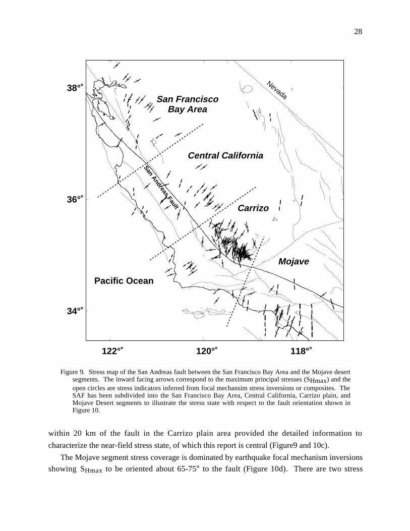
Figure 9. Stress map of the San Andreas fault between the San Francisco Bay Area and the Mojave desertsegments. The inward facing arrows correspond to the maximum principal stresses (SHmax) and theopen circles are stress indicators inferred from focal mechansim stress inversions or composites. TheSAF has been subdivided into the San Francisco Bay Area, Central California, Carrizo plain, andMojave Desert segments to illustrate the stress state with respect to the fault orientation shown inFigure 10.

within 20 km of the fault in the Carrizo plain area provided the detailed information to

characterize the near-field stress state, of which this report is central (Figure9 and 10c).

The Mojave segment stress coverage is dominated by earthquake focal mechanism inversions

showing SHmax to be oriented about 65-75° to the fault (Figure 10d). There are two stress

29

indicators from wells situated within 5 km of the fault (Hickman et al., 1988; Stock et al., 1988)

showing inconsistent results. One of the stress measurements from these shallow (~1 km) wells

indiate a SHmax direction of about 45° with respect to the fault (Stock et al., 1988).

Stress directions adjacent to the SAF along the San Francisco Bay Area, Central California,

and the Mojave desert are essentially identical with SHmax oriented about 65-85° with respect to

the fault. One possible consequence steming from the difference between the "fault-oblique"

stress state in the Carrizo plain and the "fault-normal" stress state in the Mojave desert, is that

there should be an appreciable heat-flow anomaly in the Carrizo plain area, assuming frictional

heating is occurring.

0102030405060708090

100

0 10 20 30 40 50 60Azi

mu

th w

rt f

ault

str

ike

(deg

)

Distance from SAF (km)

San Francisco Bay Area

0102030405060708090

100

0 10 20 30 40 50 60Azi

mu

th w

rt f

ault

str

ike

(deg

)

Creeping Segment in Central California

0102030405060708090

100

0 10 20 30 40 50 60Azi

mu

th w

rt f

ault

str

ike

(deg

)

Distance from SAF (km)

Distance from SAF (km)

Distance from SAF (km)

Carrizo Plain ( > 2 km deep )

0102030405060708090

100

0 10 20 30 40 50 60 70Azi

mu

th w

rt f

ault

str

ike

(deg

)

Mojave Desert

Figure 10 Comparison of stress states associated with four different segments of the San Andreas faultshown in a). Stress orientations relative to the strike of the San Andreas fault and as a function ofdistance to the fault for b) San Francisco Bay Area segment, c) Creeping segment in central California,d) Carrizo Plain segment (≥ 2 km deep), and e) Mojave Desert segment. SHmax stress indicatorsinclude those inferred from wellbore breakouts (solid) and earthquake focal mechanisms (open).Although the stress rotation along the Carrizo Plain segment is well deliniated with near-field data, theother segments do not appear to show any significant rotation within 20 km of the San Andreas fault,suggesting higher shear stress along the Carrizo Plain.

The lack of a pronounced heat-flow anomaly over the SAF within the Mojave segment

clearly indicates a low-shear stress fault segment (Figures 11 and 12). However, the heat-flow

data for the Carrizo plain area does not completely rule out the possibility of an anomaly because

30

of the step-wise increase in heat-flow when crossing the SAF from east to west (Figure heat).

This step-wise increase may be the thermal effect associated with the recent uplift of the Coast

Ranges juxtaposd to the relatively cool Great Valley (Figures 11 and 12).

Modeling

Preliminary modelling efforts explaining the transition in the stress field from fault-normal to

fault-oblique is being performed using a 2D finite element code (TECTON) and a 3-D

dislocation code. One of the important issues that any modelling approach needs to address is

whether the stress transition is a temporal feature related to the earthquake cycle. For instance,

will the present-day fault-oblique stress orientation return to fault-normal immediately following

the next major earthquake, if we assume that the stress drop associated with the event was

complete? The appealing aspect of this hypothesis is that it would explain the development of

the SAF-parallel fold axes in response to an apparent stress change to northeast SHmax direction

immediately following the major earthquake.

35 °

36 °

34 °

33 °

121 ° 120 ° 119 ° 118 ° 117 °

121 ° 120 ° 119 ° 118 ° 117 °

35 °

36 °

34 °

33 °

Carrizo Plainsegment

Mojavesegment

Southern San Joaquin Valley

SAF

SAF

Los Angeles

Bakersfield

Santa Barbara

PACIFIC OCEAN

Figure 11. Location map of heat-flow measurements adjacent to the Carrizo plain and Mojave segments ofthe San Andreas fault (after Lachenbruch and Sass, 1980).

We've attemped a very generalized simulation of this process by imposing an equivalent slip

history along the ductile and aseismic portion of the fault during several earthquake cycles, and

examined the resultant stress field in the upper locked section immediately following the

earthquake. We used a brittle-ductile rheology shown in Figure 13a using different heat-flow

31

values consistent with the scatter of values seen in the San Joaquin Valley (Figures 11 and 12).

The rheology model was designed to allow for a smooth and realistic transition from the elastic

32

CARRIZO PLAIN

81 mW/m2

61 42 - 54

9275

Surface heat-flowdue to frictionalheating

t(my)=°t=2.4

t=.3

Coast Range Thermal Mean

1.0

2.0

3.0

Hea

t fl

ow

(H

FU

)

Hea

t fl

ow

(m

W/m

2 )

42

84

126

0 20204060

Distance from San Andreas Fault (km)

0 2020 404060

Distance from San Andreas Fault (km)

1.0

2.0

3.0H

eat

flo

w (

HF

U)

Hea

t fl

ow

(m

W/m

2 )

25

50

75

100

125

USGSCal Tech

Anomaly for50 MPa friction

MOJAVE

70 mW/m2 mean

a)

b)

Figure 12 Comparison of heat-flow data from the Carrizo Plain and Mojave Desert segments. a) CarrizoPlain heat-flow, and b) Mojave desert heat-flow plotted with respect to distance from the San Andreasfault. The step increase in heat-flow across the San Andreas fault in Carrizo may not be a attributed tothe fault, but rather to a possible thermal boundary between the recently uplifted (and warm) CoastRanges to the west and the relatively cool crust in the Central Valley. This is contrasted in the Mojavedesert area where there is no marked heat-flow anomaly and the stress data suggests low shear stress(Figure 10). After Lachenbruch and Sass (1980)

33

18 20 22 24 26 28 300

10

20

30

40

50

60

Log Effective Viscosity (Pa-s)D

epth

(km

)

Granite

Diabase

Olivine

0 200 400 600 800 1000 1200 14000

10

20

30

40

50

60

Temperature (C)

Granite

Diabase

Olivine

50 mW/m2

50 mW/m2

60

60 70 80 90

708090

a) b)

Figure 13. Earth model paramters used in the finite element based on the range of heat flow measurementsseen in the San Joaquin Valley. a) Temperature profiles inferred from different heat-flow observationsshown in Figures 11 and 12. b) Effective viscosity profile used in the finite element model. Note thegradual transition between the elastic and viscoelastic layers, with the viscosity decreasing 3 orders ofmagnitude. This transition acts to avoids the stress singularity imposed by the abrupt elastic andviscoelastic boundary, but more importantly, uses model rheologies that are more geophysicallyplausible.

granite to the plastic diabase/olivine regions. The effective viscosities at this transition decreases

by about 3 orders of magnitude so as to avoid any stress singularities near the base of the locked

section of the fault (Figure 13a). Using this finite element model, we imposed a 200 and 300

year recurrence interval along a fault slipping at 35 mm/yr, below the locking depth of about 14

km and monitored the shear stress at a depth of 3 km (average depth of stress orientation data).

Our modelling tested whether the 200-300 year strain accumulation between earthquakes was

sufficient to increase the shear stresses and therefore rotate the SHmax direction to the present-

day configuration. Assuming the far-field SHmax direction is fault-normal and stress magnitudes

consistent with the industry data, the resultant superposition between the accumulated shear

stresses and the far-field stresses near the end of the cycle are insufficient to rotate the stresses to

fault-oblique. Figure 14 serves to illustrate that for the in-situ stress directions to rotate between

major earthquakes, the difference in the far-field horizontal stresses must be extremely small or

comparable in magnitude (i e., SHmax ~Shmin). Therefore, our conclusion is that the present-day

stress state is long-term and does not rotate from fault-oblique to fault-normal as a consequence

of a total stress drop earthquake.

Although the temporal shear stress accumulation i s insufficient to rotate the local stress field,

there does appear to be a stress concentration near the fault that reduces to about 50% of its peak

value at about 15-20 km from the fault (Figure 14a). Similar results have been obtained using 2-

34

D finite element and 3-D dislocation codes, in that the high shear stress concentration occurs

within 15-20 km of the fault. The stress concentrations and stress directions could be reproduced

within the area straddling the fault, however, the stress magnitudes were an order of magnitude

less than expected based on the magnitudes estimates inferred from the industry data.

Extrapolating the industry data to regions close to the fault may not be warranted, in which case,

the model boundary conditions need to be modified. A more accurate approach, which we are

exploring, is to model the fault rheology separate from the surrounding crust and impose stress-

boundary conditions on the fault instead of treating the fault and surrounding crust as

homogeneous. A similar approach of using stress boundary conditions along the fault and

displacement boundary conditions along the sides of the model were employed by Lyzenga et al.,

(1991), however, the models tested were generalized and short of performing a sensitivity

analysis.

Distance from fault (km)

0

1

2

3

4

5

0 10 20 30 40 50

She

ar S

tres

s (M

Pa)

t = 0

t = 200 yr

a)

t = 0

t = 200 yr

0

10

20

30

40

50

60

70

80

90

0 10 20 30 40 50

Distance from fault (km)

SH

max

Azi

mut

h w

.r.t.

faul

t-no

rmal

(de

g)

far-field SHmax

near-field SHmax

b)

Figure 14 Shear stress loading at a depth of 3 km over the earthquake cycle. a) Shear stresses induced byaseismic slip below the locaking depth of ~14 km at a slip rate of 35 mm/yr over a 200 year earthquakecycle, plotted as a function of distance from the fault. b) Superposition of the induced shear stressesand the far-field stress state inferred from hydraulic fracturing in the Cymric field (indicated by theshaded box > 30km from fault and oriented ~15° wrt the fault). The near-field relative stressorientations from the observed stress directions are indicated by the upper shaded box (< 20km fromfault and oriented ~55° wrt the fault). The thin and thick lines correspond to the supperposition of theinduced shear stresses and the far-field state for t=0 yr (immediately following the earthquake) andt=200 yr (immediately preceeding the earthquake). Note the lack of a rotation in the stress directionfrom "fault-oblique" before the earthquake to "fault-normal" after the earthquake.

ImplicationsThe observed transition in SHmax directions from fault-normal to fault-oblique in the near-

field regions of the San Andreas fault presents an intriguing problem in our efforts to understand

the physical mechanisms leading to earthquake nucleation and propagation. The in-situ stress

35

analysis presented in this study reflects new infomation about the possible spatial variability in

fault strength between the different segments of the San Andreas fault, which is essential for

understanding the dynamics of faulting and the earthquake process. Interestingly, our results add

a new "twist" to our current knowledge of the state of stress along this major plate boundary, and

does so by adding a few more unresolved issues.

For instance, a mechanism for explaining the San Andreas "weak" fault model has been to

appeal to elevated fault zone pore pressues (Byerlee, 1990; Rice, 1992). Our generalized

estimates of the crustal pore pressure inferred from mud weight drilling information does not

fully support or discount a high fault zone pore pressure model. Based on the coverage of data

collected a kilometer-wide fault zone with elevated pore pressure cannot be completely ruled out.

The Byerlee/Rice model cannot be fully supported by our data because none of the wells actually

penetrated the SAF proper, and the data closest to the fault indicate near-hydrostatic pore

pressures but only to depths approaching 5 km (Figure 6). Elevated pore pressures may exist at

greater depth and within the 15-20 km stress transition zone, however, these extremely wide

fault-zone dimensions would imply that the principal displacement zone for this plate boundary

would be equally wide. The remarkably narrow (<1 km) surface expression of the San Andreas

fault in the Carrizo plain is evidence against such a wide fault zone since we are not seeing a

banded shear zone 10-40 km wide.

The fault-oblique stress orientation adjacent to the Carrizo plain segment strongly suggests

that the segment may be "strong" and able to sustain relatively high shear stresses. However, if

frictional heating during the faulting process is still operative, the step-wise heat-flow profile

shown in Figure 12 does not conclusively demonstrate a "strong" fault character, but it is

suggestive. This step-wise profile could be explained by a thermal response to the recent uplift

of the Coast Ranges during the past 5 Ma or so, in which case the difference in heat flow across

the fault may be due to the juxtaposition between the warm Coast ranges and the relatively cool

San Joaquin Valley. The Heat-Flow Group at the U.S. Geolgical Survey is currently exploring

the possibility of re-entering idle wells or 'holes of opportunity' in the San Joaquin Valley,

particularly near the San Andreas fault.

Another possibilty may be that frictional sliding generates little heat because of several

dynamic weakening mechanisms associated with the earthquake rupture and propagation

processes. These include a reduction in the normal stresses or dilatational opening immediately

preceeding the propagation front (Brune, 1993); acoustic fluidization (Melosh, 1979, 1996); and

granular debris weakening (Scott, 1996). These various mechanisms have not been field tested

since they describe processes that occur at seismogenic depths and require deep in-situ

observations.

36

One of the strongest arguments supporting a fault-normal stress orientation immediately

juxtaposed to the San Andreas fault have been the Pliocene-recent fold axes oriented sub-parallel

37

Fault-Normal SHmaxLOW SHEAR STRESSES

DEPTH-AVERAGED

OVER MOST OF THE SAF

(70-100 km deep)

Fault-Oblique SHmax

RELATIVELY HIGH SHEAR

STRESSES DEPTH-AVERAGED

OVER UPPER 10-20 km of SAF

Car

rizo

Plai

n

SAF

"STRONG"(Currently

locked)

"WEAK"

10-20 km

70-100 km

Region of Aseismic Slip

SeismogenicZone

~ 70 km~ 50 km~ 20 km~ 5 km

Distance from the San Andreas Fault

De

ep

es

t "I

ma

gin

g"

Se

cti

on

s o

f th

e F

au

lt

Sh

all

ow

'im

ag

ing

"

Figure 15. Conceptual fault strength versus depth model illustrating how the distance-varying stress statemay be representative of stresses seen at specific depths along the active portions of the San Andreasfault. In-situ stress measurements collected in the far-field, which show 'fault-normal' SHmaxdirections, may be imaging the stress state depth-averaged over a depth comparable to the distance ofthe measurement. In the far-field case, fault can be considered weak when averaged over the entiredepth of the plate boundary, since most of the fault, situated below the seismogenic zone, is slippingasesimically with very little resistance to shear. Within the near-field, the stresses observed may beimaging the shallow portions of the fault comparable to the distances. For the 'fault-oblique' stressstate seen within 15-20 km of the fault, the relativley high shear stresses resolved on the fault wouldimply that the upper portions of the fault can sustain significant shear stresses.

38

to the plate boundary. The apparent discrepency between these fold axes and the fault-oblique

stress orientation is difficult to reconcile. From our modelling, it would appear that the present-

day stress state is long term, implying a stress orientation which is inconsistent with the fold axes

(assuming the fold axes reflect a structural response due to a stress direction oriented

perpendicular to the folds). This incompatibility between the fold axes and fault-oblique stress

state may be the result of deep seated folding driven by slip occurring along low-angle and SAF-

subparallel faults associated with NE-SW convergence. This would again appear to be

inconsistent with the observed stress state, unless the stress directions situated at depths greater

than our wellbore observations but within ~20 km from the SAF are subject to NE-SW

compression. Although appealing, because these blind thrust faults have not been remotely

imaged with seismic or been seismically active in recent times, we have no means of support a

fault-oblique to fault-normal transition with depth at distances less than 20 km from the SAF.

Preliminary modelling would also suggest that the region straddling the SAF, where the

"fault-oblique" stress directions are observed, may be representative of the average SAF stress

state but restricted to depths comparable to the distance where the transistion occurrs. At

distances out to 60-70 km from the fault, the observed "fault-normal" stress direction may

indicate an average stress state over the lithospheric thickness of the fault. If so, inferrences of

the stress state operative along the seismogenic portions of the SAF may only come from in-situ

stress measurements taken within 15-20 km of the SAF.

Conclusions and Recommendations

The San Andreas fault along the Carrizo plain segment appears to be characterized by a

SHmax near-field stress orientation that is fault-oblique (30-45°) to the SAF. This SHmax

orientation reflects a stress transistion from fault-normal to fault-oblique occuring between 15-20

km from the SAF. Supporting evidence includes stress-induced wellbore breakouts measured

using 4-arm caliper dip meter logs in nearly 150 wells. These wells which reached depths

approaching 7.5 km, locate between 3 and 60 km on either side of the San Andreas fault. Data

from wells located beyond 20 km or so indicates a NE-SW SHmax direction, or "fault-normal"

which is consistent with previous observations (Zoback et al., 1987; Mount and Suppe, 1987;

Castillo and Zoback, 1994). Observations of this transistion to nearly N-S SHmax direction, or

"fault-oblique" within 20 km of the SAF appears to represent a long-term stress state and not one

that fluctuates within the earthquake cycle. However, stress indicators showing a fault-oblique

direction is inconsistent with the SAF-parallel fold axes. If these folds are deep-seated, their

development may be the consequence of motion within the hanging wall of a deep blind thrust

sub-parallel to the SAF, but accommodating NE-SW convergence in response to a deeper NE-

SW SHmax direction. There is no extensive subsurface imaging of deep-seated low-angle blind

39

thrust faults that may be responsible for the folding mapped at the surface, although, a proposal

submitted to the Continental Dynamics Division of National Science Foundation to investigate

such processes and manifestations as transcompressional strain partitioning in the Carrizo plain

area .

One of the primary motivations for conducting this in-situ stress anslysis was to characterize

the possible drill sites for the San Andreas Fault Zone Drilling Project, recently proposed to

National Science Foundation, U.S. Geological Survey, Department of Energy, and the

International Continental Drilling Program (e.g., Hickman et al., 1995; Zoback et al., 1995;

Hickman et al., 1994). Although there are many industry wells drilled in the vicinity of the

Carrizo plain segement, which is one of the candidate drill sites, future efforts should focus on

attaining available well data adjacent to other sites such as the Parkfield and Mojave segments.

To better constrain our understanding of stress magnitudes along the SAF, acquiring industry

hydraulic fracturing data should be a part of that effort.

Previous modelling of the stress field adjacent to the SAF has never before included data of

the nature presented in this study. These near-field stress observations provides an

unprecedented opportunity to model the strength of the fault in a depth-dependent manner. The

limitations of the modelling attempted in this study demonstrates that the rheology of the fault

zone must be treated differently from the surrounding crust. Code development using stress

boundary conditions along the locked portions of the SAF is currently being investigated.

The importance of obtaining detailed measurements of the principal stress magnitudes

(SHmax and Shmin) within the near-field regions of the San Andreas fault is critical. The San

Andreas Fault Zone Drilling Project will certainly contribute a great deal to our understanding of

the physics of earthquakes and the processes leading to earthquake nucleation and propagation.

However, data is also needed along the other segments of the San Andreas that won't be drilled

due to budget constraints. To take advantage and re-enter existing wells drilled and later

abandoned close to the San Andreas, would enable us to more thoroughly conduct the type of in-

situ stress, heat-flow, chemical, and hydrologic experiments at reasonable depths. One such

opportunity may be to re-enter two (2) abandoned exploration wells located 3 and 5 km west of

the SAF (Carrizo Plains 1-16 and Tenneco 1-20 in Figure 3a). Each of these wells were drilled

in the early 1980's to a depth of about 2.2 km. The casing is at a depth of about 300 m, leaving

open hole conditions below to conduct the experiments just described. This field experiment

would compliment the pilot hole at Parkfield proposed for the San Andreas Fault Zone Drilling

Project.

Another aspect of this project has been to explore ways of advancing the current drilling and

measurement technologies or create new technologies critical for the success of the San Andreas

Fault Zone Drilling Project. One such project that was started as part of this LDRD project was

40

the Advanced Tiltmeter Hydraulic Fracture Imaging and Modeling project. Although this new

tiltmeter will be used for monitoring the geometry of the hydraulic fracture created during the

deep hydraulic fracturing stress measurement stages of the drilling project, it has immediate

applications in the oil and gas industry. Because nearly 50% of all production wells depend

upon hydraulic fracturing treatments to enhance hydrocarbon production, knowing the

orientation of the fracture has an important impact on designing and evaluating production field

performance. Partial funding for this tiltmeter project came from the Natural Gas and Oil

Technology Partnership in Fossil Energy within DOE.

Proposed stress, heat-flow, geochemical, and hydrologic experiments in the two abandoned

holes situated near the SAF mentioned above could also include testing of instruments being

designed at LLNL, such as the high resolution tiltmeter and slim hole seismometer. An avenue

for funding such a project could be multi-institutional, including Basic Energy Sciences at DOE

and IGPP.

41

References

Anderson, E. M., 1951, The Dynamics of Faulting and Dike Formation with Applications in

Britian, 2nd ed., Oliver and Boyd, Edinburge.

Angelier, J, 1979; Determination of the mean principal directions of stress for a given fault

population, Tectonphysics, 56, T17-T26.

Bakun, W. H. and A. G. Lindh, 1985; The Parkfield, California, earthquake prediction

experiment, Science, 229, 619-624.

Bakun, W. H. and T. V. McEvilly, 1984; Recurrence models and Parkfield, California,

earthquakes, J. Geophys. Res., 89, 3051-3058.

Barton, C. A., M. D. Zoback, and K. L. Burns, 1988, In-situ stress orientation and magnitude at

Fenton Hill geothermal site, New Mexico, Geophys. Res. Lett., 15, 467-470.

Barton, C. A., and M. D. Zoback, 1994; Stress perturbations associated with active faults

penetrated by boreholes: Possible evidence for near-complete stress drop and a new

technique for stress magnitude measurement, J. Geophys Res., 99, 9373-9390.

Blanpied, M. L., D. A. Lockner, and J. D. Byerlee, fault stability inferred from granite sliding

experiments at hydrothermal conditions, Geophys. Res. Lett., 18, 609-612, 1991.

Brace, W. F. and D. L. Kohlstedt, 1980; Limits on lithospheric stress imposed by laboratory

experiemtns, J. Geophys. Res., 85, 6248-6252.

Brune, J. N., T. L. Henyey, and R. F. Roy, 1969, Heat flow, stress, and rate of slip along the San

Andreas fault, California, J. Geophys. Res., 74, 3821-3827.

Brune, J. N., 1993, Rupture mechanism and interface separation in foam rubber models of

earthquakes: A possible solution to the heat-flow paradox and the paradox of large

overthrusts, Tectonophy., 218, 59-67.

Byerlee, J. D., 1978; Friction of rock, Pure Appl. Geophys., 116, 615-626.

Byerlee, J. D., 1990, Friction, overpressure and fault normal compression, Geophys., Res. Lett.,

17, 2109-2112.

Byerlee, J. D., A model for episodic flow of high pressure water in fault zones before

earthquakes, Geology, 21, 303-306, 1993.

Castillo, D. A., and W. L. Ellsworth, 1993, Seismotectonics of the San Andreas Fault System

Between Point Arena and Cape Mendocino in Northern California: Implications for the

Development and Evolution of a Young Transform, J. Geophys. Res., 98, 6543-6560.

Castillo, D. A., 1993, State of stress near active plate boundaries: The San Andreas fault in

northern and central California, and the Indo-Australian plate, south of Java, Ph.D.

Dissertation, Stanford University, 289pp.

42

Castillo, D. A. and Zoback, M. D., 1995, Systematic stress variations in the Southern San

Joaquin Valley and along the White Wolf Fault: Implications for the rupture mechanics of

the 1952 Ms 7.8 Kern County earthquake and its contemporary seismicity, J. Geophys. Res.,

100, 6249-6264.

Castillo, D. A. and Zoback, M. D., 1994, Systematic variations in stress state in the Southern San

Joaquin Valley: Inferences based on wellbore data and contemporary seismicity, Bull. Am.

Assoc. Petro. Geol., 78, 1257-1275.

Coulomb, C. A., 1773; Sur une application des regles de Maximis et Minimis a quelques

problemes de statique relatifs a l'Architecture, Acad. Roy. des Sciences Memoires de

math, et de physique par divers savans, 7, 343-382.

Davis, T. L., M. B Lagoe, W. J. M. Bazeley, S. A. Gordon, K. McIntosh, and J. S. Namson;

1988; Structure of the Cuyama valley, Calienta range, and Carrizo Plain and its significance

to the structural style of the southern Coast Ranges and western trnsverse Ranges, in Tertiary

tectonics and sedimentation in the Cuyama basin, San Luis Obispo, Santa Barabara, and

ventura counties, edited by W. J. M. Bazeley, Field trip Guidebook, 59, pp. 141-158, Pac.

sect. S.E.P.M.

Eberhart-Phillips, D., M. Lisowski, and M. D. Zoback, 1990; Crustal strain near the big bend of

the San Andreas Fault; Analysis of the Los Padres-Tehachapi trilaterations networks,

California, J. Geophys. Res., 95, 1139-1153.

Ellsworth, W. L., Historical Seismicity, in The San Andreas Fault System, R. E. Wallace, ed., U.

S. Geol. Surv. Professional Paper 1515, 115-152, 1990.

Grant, L. B., and A. Donnellan, 1994; 1855 and 1991 surveys of the San Andreas fault:

Implications for fault mechanics, Seis Soc. Am. Bull., 84, 241-246.

Grant, L. B., and K. E. Sieh, 1994; Paleoscismic evidence of clustered earthquakes on the San

Andreas fault in the Carrizo Plain, California, J. Geophys. Res., 99 , 6819-6841.

Henyey, T. L., and G. L. Wasserburg, 1971, Heat flow near major strike-slip faults in California,

J. Geophys. Res., 76 , 7924-7946.

Hickman, S., and M. D. Zoback, 1996; In-situ stress in a fault-hosted geothermal reservoir at

Dixie Valley, Nevada, in Faulting, Fault Sealing and Fluid Flow in Hydrocarbon

Reservoirs Conference, University of Leeds, 23-25 September, 1996, 100-101.

Hickman, S. H., M. D. Zoback, and J. H. Healy, 1988; Continuation of a deep borehole stress

mesurements profile near thge San Andreas fault: 1. Hydraulic fracturing stress

measuremetns at Hi Vista, Mojave Desert, California, J. Geophys. Res., 93, 15,183-

15,195.

43

Hickman, S., M. D. Zoback, W. L. Ellsworth, and L. W. Younker, 1994; Deep scientific

drilling in the San Andreas fault zone, Abstracts of the Workshop on Investigations of

Lithosphere Architecture and Development, Taos, NM., November 5-9, 1994.

Hickman, S., L. W. Younker, M. D. Zoback, and G. Cooper, 1995; The San Andreas Fault

Zone Drilling Project: Scientific objectives and technological challenges, J. Energy

Resources Technology, 117, 263-270.

Hubbert, M. K., and D. G. Willis, 1957; Mechanics of hydraulic fracturing, J. Pet. Technol.,

9, 153-168.

Jaeger, J. C., and N. G. W. Cook, 1979; Fundementals of Rock Mechanics, 3rd ed., 593 pp.,

Chapman and Hall London.

Jones, L. M., Focal mechanisms and the state of stress on the San Andreas fault in Southern

California, J. Geophys. Res., 93, 8869-8891, 1988.

Lachenbruch A. H., 1980, Frictional heating, fluid pressure, and the resistance to fault motion,J.

Geophys. Res., 85, 6097-6112.

Lachenbruch A. H. and J. H. Sass, 1973, Thermal-mechanical aspect of the San Andreas fault

system, in Proceedings of the Conference on the Tectonic Problems of the San Andreas fault

System, R. L. Kovach and A. Nur, eds.,Stanford University Press, 192-205.

Lachenbruch A. H. and J. H. Sass, 1980, Heat flow and energetics of the San Andreas fault zone,

J. Geophys. Res., 85 , 6185-6222.

Lachenbruch A. H. and A. McGarr, 1990, Stress and heat flow, in The San Andreas Fault

System, California, R. E. Wallace (ed.) pp. 261-277, U. S. Geol. Surv. Prof. Paper 1515.

Lachenbruch A. H. and J. H. Sass, 1992, Heat flow from Cajon Pass, fault strength and tectonic

implications, J. Geophys. Res., 97 , 4995-5015.

Lawson, A. C. and others, 1908; The California eathquake of April 18, 1906, Carnegie

Institution of Washington, Report of the earthquake investigation committee 1908.

Lyzenga, G. A., A. Raefsky, and S. G. Mulligan, 1991; Models of recurrent strike-slip cycles and

the state of crustal stress, J. Geophys. Res., 96 , 21,623-21,640.

Lisowski, M, J. C. Savage, and W. R. Prescott, 1991; The velocity field along the San Andreas

fault in central and southern California, J. Geophys. Res., 96 , 8369-8389.

McGarr, A., 1980; Some constraints on levels of shear stress in the crust from obsevations

and theory, J. Geophys Res., 85, 6231-6238.

Melosh, H. J., 1979; Acoustic fluidization: A new geologic process?, J. Geophys. Res., 84 ,

7513-7520.

Melosh, H. J., 1996; Dynamic weakening of faults by acoustic fluidization, Nature, 379 ,

601-606.

44

Moore, D. E., D. Lockner, and R. Summers, 1996; Strength of chrysotile-serpentinite gouge

under hydrothermal conditions: Can it explain a weak San Andreas fault? Geology,

Submitted.

Mount, V. S. and J. Suppe, 1987, State of stress near the San Andreas fault: Implications for

wrench tectonics, Geology, 15, 1143-1146.

Mount, V. S. and J. Suppe, 1992, Present-day stress orientations adjacent to active strike-slip

faults: California and Sumatra, J. Geophys. Res., 97, 11,995-12,013.

Oppenheimer, D. H., P. A. Reasenberg, and R. W. Simpson, 1988; Fault-plane solutions for the

1984 Morgon Hill, California earthquake sequence: Evidence for the state of stress on the

Calaveras fault, J. Geophys Res., 93, 9007-9026.

Reches, Z., G. Schubert, and C. Anderson, 1994; Modeling of periodic great earthquakes on the

San Andreas fault: Effects of nonlinear crustal rheology, J. Geophys Res., 99, 21,983-

22,000.

Rice, J. R., 1992, Fault stress states, pore pressure distributions, and the weakness of the San

Andreas fault, in Earthquake Mechanics, Rock Deformation and Transport Properties of

Rocks, edited by B. Evens and T. F. Wong, Academic Press, London, 475-503.

Scholz, C. H., 1989; Mechanics of faulting, Ann. Rev. Earth Planet. Sci, 17, 309-334.

Scott, D. R., 1996; Seismicity and stress rotation in granular model of the brittle crust,

Nature, 381, 592-595.

Sibson, R. H., 1973; Interactions between temperature and pore-fluid pressure during

earthquake faulting: A mechanism for partial and total stress relief, Nature Phys. Soc.,

243, 66-68.

Sibson, R. H., 1983; Continental fault structure and the shallow earthquake source, J. Geol.

Soc. London, 140, 741-767.

Sieh, K. E., and R. H. Jahns, 1984; Holocene activity of the San Andreas Fault at Wallace

Creek, California, Geol. Soc. Amer. Bull., 95, 883-896.

Sims, J. D., 1993; Chronology of displacement on the San Andreas fault in Central california:

Evidence from reversed positions of exotic rock bodies near Parkfield, California, in The

San Andreas fault system; displacement, palinspastic reconstruction, and geologic

evolution, edited by R. E. Powell, R. J. Weldon II and J. C. Matti, Memoir, 178, pp. 231-

256, Geol. Soc. Amer.

Stock J. H., and J. H. Healy, 1988; Continuation of a deep borehole stress mesurements

profile near thge San Andreas fault: 2. Hydraulic fracturing stress measuremetns at Black

Butte, Mojave Desert, California, J. Geophys. Res., 93, 15,196-15,210.

45

Stock, J. M., J. H. Healy, S. H. Hickman, and M. D. Zoback, 1985, Hydraulic fracturing

stress measurements at Yucca Mountain Nevada, and relationships to the regional sstress

field, J. Geophys Res., 90, 8691-8706.

Vernik, L., and M. D. Zoback, 1992; Estimations of the maximum horizontal principal stress

magnitude from stress-induced wellbore breakouts in the Cajon Pass scientific research

borehole, J. Geophys Res., 97, 5109-5119.

Wallace, R. E., 1968; Noteson stream channels offset by the San Andreas fault, souther Coast

Ranges, California, in Proceedings of the conference on geologic problems of the San

Andreas Fault, edited by W. R. Dickinson and A. Grant, 11 pp, Stanford University

Publications in the Geologic Sciences.

Wallace, R. E., 1990; General Features and Geomorphic Expression, in The San Andreas Fault

System, R. E. Wallace, ed., U. S. Geol. Surv. Professional Paper 1515, 3-21.

Zoback, M. D., and S. Hickman, 1982; In situ study of the physical mechanisms controlling

induced seismicity in Montcello reservoir, South Carolina, J. Geophys Res., 87, 6959-

6974.

Zoback, M. D., and J. H. Healy, 1984; Friction, faulting and in-situ stress, Annales

Geophysicae, 2, 689-698.

Zoback, M. D., M. L. Zoback, V. S. Mount, J. Suppe, J. P. Eaton, J. H. Healy, D. Oppenheimer,

P. Reasenberg, L. Jones, C. B. Raleigh, I. G. Wong, O. Scotti, and C. Wentworth, 1987, New

evidence on the state of stress of the San Andreas fault system, Science, 238, 1105-1111.

Zoback, M. D., and G. C. Beroza, 1993, Evidence for near-frictionless faulting in the 1989 (M

6.9) Loma Prieta, California, earthquake and its aftershocks, Geology, 21, 181-185.

Zoback, M. L. and Zoback, M. D., Tectonic stress field of the conterminous United States: Geol.

Soc. Am. Mem., 172, 523-539, 1991.

Zoback, M. D., S. Hickman, L. W. Younker, and W. L. Ellsworth, 1995; Strong plates and weak

plate boundaries: Reconciling relative plate motions, plate-driving forces and intraplate

seismicity through scientific drilling, Abstracts XXI General Assembly of the International

Union of Geodesy and Geophysics, Boulder, CO.

Technical Inform

ation Departm

ent • Lawrence Liverm

ore National Laboratory

University of C

alifornia • Livermore, C

alifornia 94551