
A High Precision Measurement of the Proton Charge Radius ...
232
A High Precision Measurement of the Proton Charge Radius at JLab by Weizhi Xiong Department of Physics Duke University Date: Approved: Haiyan Gao, Advisor Phillip S. Barbeau Shailesh Chandrasekharan Stephen W. Teitsworth Christopher Walter Dissertation submitted in partial fulfillment of the requirements for the degree of Doctor of Philosophy in the Department of Physics in the Graduate School of Duke University 2020
Transcript of A High Precision Measurement of the Proton Charge Radius ...

A High Precision Measurement of the Proton Charge Radius
at JLab
by
Weizhi Xiong
Department of PhysicsDuke University
Date:Approved:
Haiyan Gao, Advisor
Phillip S. Barbeau
Shailesh Chandrasekharan
Stephen W. Teitsworth
Christopher Walter
Dissertation submitted in partial fulfillment of therequirements for the degree of Doctor of Philosophy
in the Department of Physicsin the Graduate School of
Duke University
2020

ABSTRACT
A High Precision Measurement of the Proton Charge Radius
at JLab
by
Weizhi Xiong
Department of PhysicsDuke University
Date:Approved:
Haiyan Gao, Advisor
Phillip S. Barbeau
Shailesh Chandrasekharan
Stephen W. Teitsworth
Christopher Walter
An abstract of a dissertation submitted in partial fulfillment of therequirements for the degree of Doctor of Philosophy
in the Department of Physicsin the Graduate School of
Duke University
2020

Copyright c© 2020 by Weizhi Xiong
All rights reserved

Abstract
The elastic electron-proton (e−p) scattering and the spectroscopy of hydrogen atoms
are the two traditional methods to determine the proton charge radius (rp). In 2010,
a new method using muonic hydrogen (µH)1 spectroscopy reported a rp result that
was nearly ten times more precise but significantly smaller than the values from the
compilation of all previous rp measurements. This discrepancy is often referred to
as the “proton charge radius puzzle”. In order to investigate the puzzle, the PRad
experiment (E12-11-1062) was first proposed in 2011 and performed in 2016 in Hall
B at the Thomas Jefferson National Accelerator Facility, with both 1.1 and 2.2 GeV
electron beams. The experiment measured the e− p elastic scattering cross sections
in an unprecedented low values of momentum transfer squared region (Q2 = 2.1 ×
10−4−0.06 (GeV/c)2), with a sub-percent precision. The PRad experiment utilized a
calorimetric method that was magnetic-spectrometer-free. Its detector setup included
a large acceptance and high resolution calorimeter (HyCal), and two large-area, high-
spatial-resolution Gas Electron Multiplier (GEM) detectors. To have a better control
over the systematic uncertainties, the absolute e−p elastic scattering cross section was
normalized to that of the well-known Møller scattering process, which was measured
simultaneously during the experiment. For each beam energy, all data with different
Q2 were collected simultaneously with the same detector setup, therefore sharing
the same integrated luminosity. The windowless H2 gas-flow target utilized in the
experiment largely removed a typical background source, the target cell windows. The
proton charge radius was determined as rp = 0.831±0.007stat.±0.012syst. fm, which is
smaller than the average rp from previous e−p elastic scattering experiments, but in
agreement with the µH spectroscopic results within the experimental uncertainties.
1A muonic hydrogen has its orbiting electron replaced by a muon.
2Spokespersons: A. Gasparian (contact), H. Gao, M. Khandaker, D. Dutta
iv
Acknowledgements
First of all, I would like to sincerely thank my advisor, Prof. Haiyan Gao, for giving
me the opportunity to work on this project, and for her generous support not only for
me but also for the entire PRad experiment. She not only guided me through various
difficulties of this project but also provided me the help I needed for my personal life
during my graduate school, even though she was very busy all the time. I believe the
best way I can appreciate all these is by working as hard as I can.
I would also like to thank all the members in the PRad collaboration, especially se-
nior physicists: Dr. Gasparian, Dr. Khandaker, Dr. Dutta, Dr. Liyanage, Dr. Pasyuk
and Dr. Higinbotham for continuously giving me valuable suggestions throughout the
years. I would like to thank all the graduate students who worked on this experiment,
including Chao Peng, Xinzhan Bai, Li Ye, and Yang Zhang. I enjoyed all the time
we spent together in order to solve various problems, to build and test our detectors,
to run the experiment and to overcome various difficulties in the analysis. I would
like to express my great appreciation for all the postdoc of this experiment, including
Xuefei Yan, Chao Gu, Mehdi Meziane, Vladimir Khachatryan, Maxime Levillain and
Zhihong Ye, for their important contributions to various aspects of this experiment,
and for their valuable guidance and suggestions for the analysis. I would like to thank
especially Xuefei Yan and Chao Gu, who had worked very closely with me through
out the years, and had a lot of fruitful discussions about the analysis. Xuefei Yan
has developed a machine learning algorithm for rejecting the cosmic background for
the PRad experiment, and studied the robust fitters for the PRad result. Chao Gu
is one of the most important contributors for the PRad simulation software package
and spent a lot of efforts on the event generators and radiative corrections.
Lastly I would like to thank Chao Peng, who has been one of the most important
v

contributors since the early development and preparation stage of the PRad experi-
ment, and has developed the data analysis software framework for the experiment. I
appreciate all the help and suggestions he gave me during my years in the graduate
school.
vi

Contents
Abstract iv
Acknowledgements v
List of Figures x
List of Tables xviii
List of Abbreviations xix
1 Introduction 1
2 Physics Background 8
2.1 Unpolarized electron-proton scattering . . . . . . . . . . . . . . . . . 8
2.2 Proton Form Factors . . . . . . . . . . . . . . . . . . . . . . . . . . . 14
2.3 Proton Form Factors from e− p Scattering Experiments . . . . . . . 17
2.3.1 Unpolarized Measurements . . . . . . . . . . . . . . . . . . . . 18
2.3.2 Polarization Transfer Measurements . . . . . . . . . . . . . . . 23
2.3.3 Double Polarization Measurements . . . . . . . . . . . . . . . 25
2.4 Hydrogen Sepctroscopy . . . . . . . . . . . . . . . . . . . . . . . . . . 31
3 The Experiment 38
3.1 Overview . . . . . . . . . . . . . . . . . . . . . . . . . . . . . . . . . . 38
3.2 The electron beam . . . . . . . . . . . . . . . . . . . . . . . . . . . . 40
3.3 Target system . . . . . . . . . . . . . . . . . . . . . . . . . . . . . . . 43
3.4 Gas Electron Multiplier . . . . . . . . . . . . . . . . . . . . . . . . . . 46
3.5 Hybrid Calorimeter . . . . . . . . . . . . . . . . . . . . . . . . . . . . 49
3.6 Hall B Photon Tagger . . . . . . . . . . . . . . . . . . . . . . . . . . 54
vii
3.7 Triggers and Data Acquisition . . . . . . . . . . . . . . . . . . . . . . 55
4 Data Analysis 61
4.1 Overview . . . . . . . . . . . . . . . . . . . . . . . . . . . . . . . . . . 61
4.2 Event Reconstruction . . . . . . . . . . . . . . . . . . . . . . . . . . . 66
4.3 Calibration . . . . . . . . . . . . . . . . . . . . . . . . . . . . . . . . 69
4.3.1 Energy Calibration . . . . . . . . . . . . . . . . . . . . . . . . 69
4.3.2 Position Calibration . . . . . . . . . . . . . . . . . . . . . . . 81
4.4 Event Selection . . . . . . . . . . . . . . . . . . . . . . . . . . . . . . 84
4.5 Background Subtraction . . . . . . . . . . . . . . . . . . . . . . . . . 91
4.5.1 Background from Beam-Line . . . . . . . . . . . . . . . . . . . 92
4.5.2 Background from Inelastic e− p channels . . . . . . . . . . . . 97
4.5.3 Background from photon induced GEM hits . . . . . . . . . . 102
4.5.4 Background from Multiple Scattering of Small Angle Events . 102
4.6 Efficiency of GEM . . . . . . . . . . . . . . . . . . . . . . . . . . . . 105
4.7 Simulation . . . . . . . . . . . . . . . . . . . . . . . . . . . . . . . . . 116
4.8 Angular Resolution and Q2 Resolution . . . . . . . . . . . . . . . . . 120
4.9 Cross Section Extraction . . . . . . . . . . . . . . . . . . . . . . . . . 124
4.9.1 (e− p) /(e− e) Ratio . . . . . . . . . . . . . . . . . . . . . . . 124
4.9.2 Radiative Corrections . . . . . . . . . . . . . . . . . . . . . . . 128
4.9.3 Born Level e− p Elastic Scattering Cross Section . . . . . . . 131
4.10 Systematic Uncertainties on Cross Section . . . . . . . . . . . . . . . 136
4.10.1 Systematic Uncertainties Associated with Cuts . . . . . . . . . 137
4.10.2 Systematic uncertainties from Experimental Conditions . . . . 140
4.10.3 Systematic uncertainties from Models . . . . . . . . . . . . . . 156
viii

4.11 Proton Electric Form Factor Extraction . . . . . . . . . . . . . . . . . 159
5 Radius Extraction 163
5.1 Search for Robust Fitters . . . . . . . . . . . . . . . . . . . . . . . . . 164
5.2 Systematic Uncertainty on the Radius . . . . . . . . . . . . . . . . . 167
5.3 Proton Charge Radius Result . . . . . . . . . . . . . . . . . . . . . . 170
6 Possible Improvements on the Result 181
7 Conclusion 192
A Cross Section and Form Factor Data 198
Bibliography 203
Biography 213
ix
List of Figures
1.1 Proton charge radius results from recent experiments [1, 5, 6, 18, 19,20, 22] and world data compilations [4, 7]. . . . . . . . . . . . . . . . 3
2.1 The Born level (one photon exchange) Feynman diagram for the e− pelastic scattering. . . . . . . . . . . . . . . . . . . . . . . . . . . . . . 9
2.2 Diagram for the e− p elastic scattering. . . . . . . . . . . . . . . . . 9
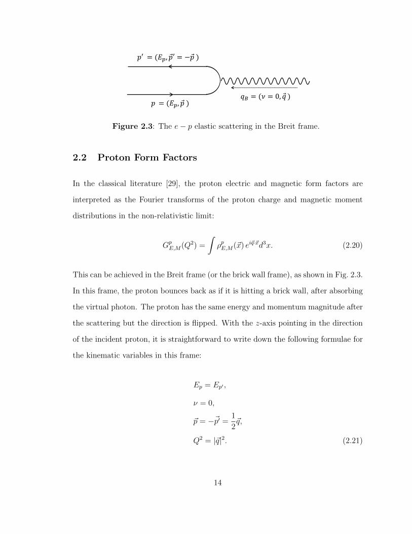
2.3 The e− p elastic scattering in the Breit frame. . . . . . . . . . . . . 14
2.4 An example demonstrating the Rosenbluth separation technique. . . . 19
2.5 The extracted proton GpE and Gp
M parameterizations from the Mainzexperiment [5]. . . . . . . . . . . . . . . . . . . . . . . . . . . . . . . 21
2.6 The proton electric form factor results from the Saskatoon experiment,obtained by measuring the recoil proton from the elastic e−p scattering. 22
2.7 Proton form factor ratio measurements in the low Q2 region, obtainedusing the polarized e− p elastic scatterings. . . . . . . . . . . . . . . 24
2.8 Proton form factor ratios obtained using the Rosenbluth separationmethod, and polarization transfer measurements. . . . . . . . . . . . 26
2.9 Born level diagram for the double polarization e− p elastic scattering. 27
2.10 The BLAST detector and proton form factor ratio results from theBLAST experiment. . . . . . . . . . . . . . . . . . . . . . . . . . . . 29
2.11 Compilation of the GpE/GD (top plot) and Gp
M/(µpGD) at BLASTkinematics. . . . . . . . . . . . . . . . . . . . . . . . . . . . . . . . . 30
2.12 Muonic hydrogen energy levels, transitions and de-excitations. . . . . 36
2.13 The measured frequency for 2SF=11/2 - 2PF=2
3/2 transition of a muonichydrogen atom. . . . . . . . . . . . . . . . . . . . . . . . . . . . . . . 37
x

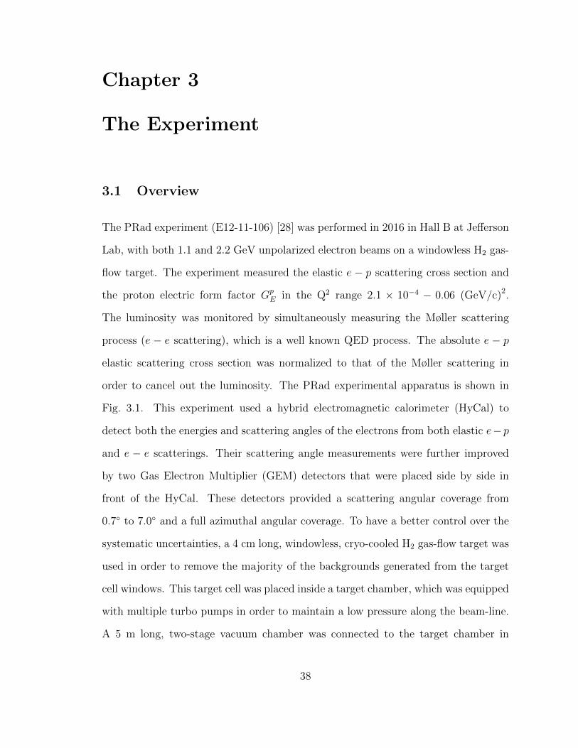
3.1 Schematic layout of the PRad experimental setup in Jeferson Lab, HallB. . . . . . . . . . . . . . . . . . . . . . . . . . . . . . . . . . . . . . 39
3.2 An overview of CEBAF at Jefferson Lab. . . . . . . . . . . . . . . . . 41
3.3 Example of the beam profile measured by harps during the PRad ex-periment. . . . . . . . . . . . . . . . . . . . . . . . . . . . . . . . . . 42
3.4 The target cell used in the PRad experiment. The cell is a cylinderwith 4 cm length and 5 cm in diameter. . . . . . . . . . . . . . . . . . 43
3.5 3D view of the PRad target system. . . . . . . . . . . . . . . . . . . . 45
3.6 Working principle of GEM. . . . . . . . . . . . . . . . . . . . . . . . . 47
3.7 The electric field produced by a GEM foil. . . . . . . . . . . . . . . . 47
3.8 PRad GEM detectors in the Experimental Equipment Lab at JLab. 48
3.9 Design for the PRad GEM detector. . . . . . . . . . . . . . . . . . . . 49
3.10 The hit positions of e−p elastic scattering events on GEMs are shownalong one of the strip directions. . . . . . . . . . . . . . . . . . . . . . 50
3.11 Front view of the HyCal electromagnetic calorimeter. . . . . . . . . . 51
3.12 PbWO4 and Pb-glass modules of HyCal calorimeter. . . . . . . . . . . 52
3.13 Front view of HyCal. . . . . . . . . . . . . . . . . . . . . . . . . . . . 53
3.14 The bremsstrahlung photon tagger in Hall B at Jefferson Lab. . . . . 55
3.15 The configuration of the PRad DAQ system for the production runs. 57
3.16 Summing all 52 signals from the UVA120A modules, using NIM modules. 57
4.1 The flow chart for the data analysis procedure. . . . . . . . . . . . . . 65
4.2 Examples of HyCal cluster reconstruction for an event that has twomaxima in the same group. . . . . . . . . . . . . . . . . . . . . . . . 68
xi
4.3 The HyCal movement during the calibration runs. . . . . . . . . . . . 70
4.4 The ratio between the reconstructed energy Erec and the beam energyEγ, for beam energy around 550 MeV. . . . . . . . . . . . . . . . . . 71
4.5 The non-linearity behavior of a PbWO4 module W213 and a Pb-glassmodule G507. . . . . . . . . . . . . . . . . . . . . . . . . . . . . . . . 72
4.6 The energy resolution of the PbWO4 detector. . . . . . . . . . . . . . 73
4.7 The trigger efficiency for PbWO4 and Pb-glass detectors, as a functionof the incident photon beam energy. . . . . . . . . . . . . . . . . . . . 74
4.8 The reconstructed energy Erec over the expected energy Eexp for thee− p elastic scattering and the e− e elastic scattering. . . . . . . . . 75
4.9 The non-uniformity in the HyCal reconstructed energy for e−p eventsin a PbWO4 module W521 and a Pb-glass module G238. . . . . . . . 77
4.10 The non-linearity correction function of a Pb-glass module from thePrimEx-II experiment. . . . . . . . . . . . . . . . . . . . . . . . . . . 78
4.11 The HyCal gain factors for the module W103 and the average of allHyCal modules as a function of run number. . . . . . . . . . . . . . . 79
4.12 The reconstructed elastic peak positions from each run over the aver-aged peak position from all the runs. . . . . . . . . . . . . . . . . . . 80
4.13 A diagram that indicates the azimuthal angles (φe1 and φe2) of thescattered electrons from the e− e scattering process. . . . . . . . . . 82
4.14 The co-planarity and vertex z distributions, reconstructed using theGEM reconstructed coordinates. . . . . . . . . . . . . . . . . . . . . . 83
4.15 ∆R distributions between the HyCal and GEM reconstructed hits. . . 85
4.16 The reconstructed energy as a function of the reconstructed scatteringangle. . . . . . . . . . . . . . . . . . . . . . . . . . . . . . . . . . . . 87
4.17 The co-planarity and vertex z distributions, reconstructed using theHyCal reconstructed coordinates. . . . . . . . . . . . . . . . . . . . . 90
xii

4.18 Main target configurations during the PRad data taking. . . . . . . . 93
4.19 The counts from the runs with different target configuration over thatfrom the full target runs, for the 2.2 GeV beam setting. . . . . . . . . 95
4.20 The counts from the runs with different target configuration over thatfrom the full target runs, for the 1.1 GeV beam setting. . . . . . . . . 96
4.21 The normalized ratios between e− p and e− e counts after the back-ground subtraction, as a function of the run number. . . . . . . . . . 98
4.22 The reconstructed energy spectrum from the 2.2 GeV data and thesimulation for part of the PbWO4 and Pb-glass detector regions. . . . 99
4.23 χ2 from Eq. 4.27, as a function of scale factor and stretch factor forthe 2.2 GeV beam energy setting. . . . . . . . . . . . . . . . . . . . . 101
4.24 The ratio between background counts due to the events with scatteringangles from 0.2 to 0.6 and the total counts using the PRad simulation.104
4.25 Super ratio between the live charge and total time. . . . . . . . . . . 107
4.26 GEM efficiencies as a function of the size of the kinematic cuts. . . . 108
4.27 GEM efficiencies measured using the e− p and e− e events. . . . . . 110
4.28 The GEM efficiencies obtained from the PRad simulation. . . . . . . 112
4.29 GEM efficiency cancellation and correction error. . . . . . . . . . . . 113
4.30 The GEM efficiency measured using 2.2 GeV e−p events, from regionsthat have no GEM spacers. . . . . . . . . . . . . . . . . . . . . . . . 114
4.31 The e − p to e − e ratios between the data and the simulation fromdifferent quadrants. . . . . . . . . . . . . . . . . . . . . . . . . . . . . 115
4.32 Feynman diagrams calculated in the generator [79] for the e−p elasticscattering. . . . . . . . . . . . . . . . . . . . . . . . . . . . . . . . . . 117
4.33 Feynman diagrams calculated in the generator [79] for the e−e elasticscattering. . . . . . . . . . . . . . . . . . . . . . . . . . . . . . . . . . 118
xiii

4.34 Feynman diagrams calculated in the generator [31] for the e−p elasticscattering. . . . . . . . . . . . . . . . . . . . . . . . . . . . . . . . . . 119
4.35 The reconstructed energy spectrum from the data and simulations forthe 2.2 GeV beam energy setting. . . . . . . . . . . . . . . . . . . . . 121
4.36 The simulated gas density profile along the beam line by COMSOLMultiphysics R© simulation package. . . . . . . . . . . . . . . . . . . . 122
4.37 The polar-angle and Q2 resolutions of the experimental setup. . . . . 123
4.38 The super ratios obtained using the integrated Møller method and thebin-by-bin method. . . . . . . . . . . . . . . . . . . . . . . . . . . . . 127
4.39 The comparison between super ratios obtained when using only thePbWO4 modules and when using all modules. . . . . . . . . . . . . . 128
4.40 The elastic e − p counts from the simulation, obtained with differentEminγ and Emax
γ cuts, for the 1.1 GeV beam energy setting. . . . . . . 130
4.41 The iterative procedure for the radiative correction. . . . . . . . . . . 132
4.42 The super ratios before and after the iteration process. . . . . . . . . 133
4.43 The relative difference in the cross sections before and after the itera-tion process. . . . . . . . . . . . . . . . . . . . . . . . . . . . . . . . . 134
4.44 The Born level differential cross sections for the e−p elastic scatteringfrom the 1.1 GeV and 2.2 GeV data sets. . . . . . . . . . . . . . . . . 135
4.45 The reduced cross section as defined in Eq. 4.31, for the 1.1 GeV and2.2 GeV data sets. . . . . . . . . . . . . . . . . . . . . . . . . . . . . 135
4.46 Total relative systematic uncertainties for the e − p elastic scatteringcross sections for the 1.1 and 2.2 GeV data sets. . . . . . . . . . . . . 138
4.47 The variations of the super ratio results when changing the size of thekinematic cuts for the 1.1 GeV e− p event selection. . . . . . . . . . 141
4.48 The variations of the super ratio results when changing the size of thekinematic cuts for the 2.2 GeV e− p event selection. . . . . . . . . . 142
xiv

4.49 The variations of the super ratio results when changing the size of theenergy cuts for the 1.1 GeV e− e event selection. . . . . . . . . . . . 143
4.50 The variation of the super ratio results when changing the size of theenergy cuts for the 2.2 GeV e− e event selection. . . . . . . . . . . . 144
4.51 The z-vertex distributions from the 2.2 GeV data, and simulationsusing the gas profiles with min. tails and max. tails. . . . . . . . . . . 148
4.52 The e− p to e− e ratios obtained with the gas profile with max. tailsover those with the min. tails, in the case of the 2.2 GeV energy setting.149
4.53 The e−p to e− e ratios from simulations with different beam energiesover those obtained with the nominal beam energy. . . . . . . . . . . 152
4.54 Correlation between the beam energies and the determined z positionof GEM-I. . . . . . . . . . . . . . . . . . . . . . . . . . . . . . . . . . 152
4.55 The e− p to e− e ratios from different simulations with shifted GEMpositions over those obtained from the standard simulation. . . . . . . 155
4.56 Relative systematic uncertainties for the cross sections due to internalradiative corrections for the e− p and e− e. . . . . . . . . . . . . . . 157
4.57 Relative systematic uncertainties for the cross sections due to the in-elastic e− p contribution. . . . . . . . . . . . . . . . . . . . . . . . . 159
4.58 Different GpM parameterizations and the relative difference between the
extracted GpE using these Gp
M parameterizations. . . . . . . . . . . . . 161
4.59 The total relative systematic uncertainties of the proton electric formfactor Gp
E for the 1.1 and 2.2 GeV data sets. . . . . . . . . . . . . . . 162
4.60 The extracted proton electric form factors GpE from both the 1.1 and
2.2 GeV data sets. . . . . . . . . . . . . . . . . . . . . . . . . . . . . 162
5.1 Robust fitter test results for the dipole, monopole and Gaussian fitters. 167
5.2 Robust fitter test results for the multi-parameter polynomial expansionof Q2. . . . . . . . . . . . . . . . . . . . . . . . . . . . . . . . . . . . 168
xv
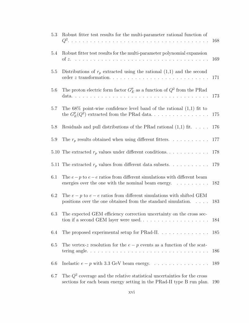
5.3 Robust fitter test results for the multi-parameter rational function ofQ2. . . . . . . . . . . . . . . . . . . . . . . . . . . . . . . . . . . . . . 168
5.4 Robust fitter test results for the multi-parameter polynomial expansionof z. . . . . . . . . . . . . . . . . . . . . . . . . . . . . . . . . . . . . 169
5.5 Distributions of rp extracted using the rational (1,1) and the secondorder z transformation. . . . . . . . . . . . . . . . . . . . . . . . . . . 171
5.6 The proton electric form factor GpE as a function of Q2 from the PRad
data. . . . . . . . . . . . . . . . . . . . . . . . . . . . . . . . . . . . . 173
5.7 The 68% point-wise confidence level band of the rational (1,1) fit tothe Gp
E(Q2) extracted from the PRad data. . . . . . . . . . . . . . . . 175
5.8 Residuals and pull distributions of the PRad rational (1,1) fit. . . . . 176
5.9 The rp results obtained when using different fitters. . . . . . . . . . . 177
5.10 The extracted rp values under different conditions. . . . . . . . . . . . 178
5.11 The extracted rp values from different data subsets. . . . . . . . . . . 179
6.1 The e−p to e−e ratios from different simulations with different beamenergies over the one with the nominal beam energy. . . . . . . . . . 182
6.2 The e− p to e− e ratios from different simulations with shifted GEMpositions over the one obtained from the standard simulation. . . . . 183
6.3 The expected GEM efficiency correction uncertainty on the cross sec-tion if a second GEM layer were used. . . . . . . . . . . . . . . . . . . 184
6.4 The proposed experimental setup for PRad-II. . . . . . . . . . . . . . 185
6.5 The vertex-z resolution for the e− p events as a function of the scat-tering angle. . . . . . . . . . . . . . . . . . . . . . . . . . . . . . . . . 186
6.6 Inelastic e− p with 3.3 GeV beam energy. . . . . . . . . . . . . . . . 189
6.7 The Q2 coverage and the relative statistical uncertainties for the crosssections for each beam energy setting in the PRad-II type B run plan. 190
xvi

6.8 Robust fitter test results for the rational (1,1) fitter, based on thePRad-II type B. . . . . . . . . . . . . . . . . . . . . . . . . . . . . . . 191
6.9 Projected total uncertainties on rp for PRad-II type A and type B runplans. . . . . . . . . . . . . . . . . . . . . . . . . . . . . . . . . . . . 191
7.1 The rp extracted from the PRad data, shown along with the othermeasurements of rp since 2010 and the CODATA recommended values. 193
7.2 Comparison between PRad GpE and a number of previously measured
GpE data sets [15, 36, 37]. . . . . . . . . . . . . . . . . . . . . . . . . . 195
7.3 The rp extracted from the PRad data, and other measurements oranalyses of rp from e− p elastic scattering experiments. . . . . . . . . 197
xvii
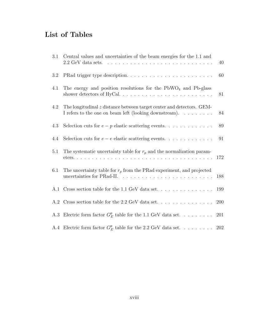
List of Tables
3.1 Central values and uncertainties of the beam energies for the 1.1 and2.2 GeV data sets. . . . . . . . . . . . . . . . . . . . . . . . . . . . . 40
3.2 PRad trigger type description. . . . . . . . . . . . . . . . . . . . . . . 60
4.1 The energy and position resolutions for the PbWO4 and Pb-glassshower detectors of HyCal. . . . . . . . . . . . . . . . . . . . . . . . . 81
4.2 The longitudinal z distance between target center and detectors. GEM-I refers to the one on beam left (looking downstream). . . . . . . . . 84
4.3 Selection cuts for e− p elastic scattering events. . . . . . . . . . . . . 89
4.4 Selection cuts for e− e elastic scattering events. . . . . . . . . . . . . 91
5.1 The systematic uncertainty table for rp and the normalization param-eters. . . . . . . . . . . . . . . . . . . . . . . . . . . . . . . . . . . . . 172
6.1 The uncertainty table for rp from the PRad experiment, and projecteduncertainties for PRad-II. . . . . . . . . . . . . . . . . . . . . . . . . 188
A.1 Cross section table for the 1.1 GeV data set. . . . . . . . . . . . . . . 199
A.2 Cross section table for the 2.2 GeV data set. . . . . . . . . . . . . . . 200
A.3 Electric form factor GpE table for the 1.1 GeV data set. . . . . . . . . 201
A.4 Electric form factor GpE table for the 2.2 GeV data set. . . . . . . . . 202
xviii

List of Abbreviations
ADC Analog-to-Digital Convertor
BPM Beam Position Monitor
CEBAF Continuous Electron Beam Accelerator Facility
CODA CEBAF Online Data Acquisition
DAQ Data Acquisition System
EPICS Experimental Physics and Industrial Control System
FEC Front-End Concentrator cards
GEM Gas Electron Multiplier
HyCal Hybrid Calorimeter
PMT Photon Multiplier Tube
QCD Quantum Chromodynamics
QED Quantum Electrodynamics
RMS Root-Mean-Square
SRS Scalable Readout System
TDC Time-to- Digital Convertor
TPC Time Projection Chamber
TPE Two Photon Exchange
TI Trigger Interface
xix

Chapter 1
Introduction
Nucleons (protons and neutrons) are primary building blocks of the visible universe,
and they make up over 99.9% of visible matter. It is important to understand the
basic properties of a proton, such as its root-mean-square (RMS) charge radius1 rp.
It is related to the spacial distribution of the proton’s charge, which is carried by
the quarks. A precise knowledge of rp is certainly important to our understanding
about how Quantum Chromodynamics (QCD) - the theory of the strong interaction
- works in the non-perturbative region. This quantity is also an important input to
the bound state Quantum Electrodynamics (QED) calculations of atomic hydrogen
energy levels. For instance, for a muonic hydrogen (µH) atom, the proton charge
radius affects the Lamb shift between 2S1/2 and 2P1/2 energy levels by as much as
2% [1]. It also impacts the determination of the Rydberg constant (R∞), which is one
of the most precisely measured quantities in physics. A high precision measurement
of the Rydberg constant comes from the exact same type of experiments where the
proton charge radius can be determined, so that they are highly correlated.
There are two well-established methods to measure the proton charge radius.
The more traditional method is the electron-proton (e− p) elastic scattering exper-
iment [2], in which one measures the elastic e − p scattering cross section and then
extracts the proton electric form factor GpE. The proton charge radius can be de-
termined from the slope of GpE as the four-momentum transfer squared Q2 goes to
1It is often referred to as the proton charge radius in this dissertation
1

zero [2]:
〈r2p〉 ≡ −6
dGpE(Q2)
dQ2
∣∣∣∣Q2=0
(1.1)
The second method is hydrogen spectroscopy [3], in which one measures the transition
frequency between two energy levels of a hydrogen atom. These energy levels are
affected by the proton charge distribution, and one can determine the proton charge
radius from the measured transition frequency, combined with the state-of-the-art
bound state QED calculations. The hydrogen Lamb shift has been the transition
often adopted for this purpose. The physics background and various techniques used
in these two types of methods will be discussed in the next chapter.
Results of rp obtained with these two methods generally agreed with each other
prior to 2010. Based on CODATA-2010 [4], the rp results are 0.8758(77) fm and
0.895(18) fm, obtained from the compilations of previous hydrogen spectroscopy and
e − p elastic scattering experiments, respectively. This agreement was further rein-
forced in the same year by the result from the high precision e− p elastic scattering
experiment at Mainz Microtron (MAMI) [5]. It measured about 1400 cross section
data points, covering Q2 from 0.004 to 1 (GeV/c)2. The extracted rp from the Mainz
experiment is 0.8791(79) fm. Combining these results, CODATA-2010 gave the rec-
ommended value for rp as
rp = 0.8775± 0.0051 fm. (1.2)
However, also in 2010, a new rp result was reported based on a novel method using
the muonic hydrogen (µH) spectroscopy [1]. A µH atom has its orbiting electron
replaced by a muon, which is about 200 times heavier than an electron. As a result,
the muon orbits much closer to the proton and is more sensitive to the proton charge
2

[fm]p
Proton charge radius r0.78 0.8 0.82 0.84 0.86 0.88 0.9 0.92
CODATA-2010
CODATA-2014H spect.)µAntognini 2013 (
H spect.)µPohl 2010 (
Beyer 2017 (H spect.)
Fleurbaey 2018 (H spect.)
Bernauer 2010 (ep scatt.)
Mihovilovic 2019(ep scatt.)
Bezginov 2019 (H spect.)
σ7
Figure 1.1: Proton charge radius results from recent experiments [1, 5, 6, 18, 19,20, 22] and world data compilations [4, 7].
radius. The reported result from this experiment is
rp = 0.84184± 0.00067 fm, (1.3)
with an unprecedented precision of better than 0.1%. However, this value is 7σ
smaller than the CODATA -2010 recommended value (see Fig. 1.1), and it was con-
firmed by a second µH result reported in 2013 [6], which gave
rp = 0.84087± 0.00039 fm. (1.4)
This discrepancy between the electronic and muonic measurements was unexpected,
as the µ− p and e− p interactions were expected to be the same as described by the
Standard Model. The discrepancy is often referred to as the “proton charge radius
puzzle”, and has triggered intensive experimental and theoretical efforts to resolve
this puzzle.
3

The bound state QED calculations for muonic hydrogen have been scrutinized
and refined after the puzzle, yet no convincing evidence could be found to explain
the discrepancy [8]. New physics related to lepton2 universality violation has been
proposed [9], which suggests that new particles that couple stronger to the muon
and proton can possibly resolve the puzzle. Constraints from other physics such
as the muon (g − 2)µ, Kaon decay and the hyper-fine structure measurement in
the muonic hydrogen [9], put unusual requirements on the properties of these new
particles, though not denying their existence. The definition of the proton charge
radius (Eq. 1.1) has been examined rigorously in both the spectroscopic and scattering
theories [10]. The same GpE slope at Q2 = 0, measured by the elastic scattering
experiments, is shown to be responsible for the finite proton size effect in the hydrogen
spectroscopy. However, as pointed out also in Ref. [10], the rp defined in Eq. 1.1 is
not strictly related to the second moment of the proton charge density distribution.
Meanwhile, for e− p scattering, the proper Q2 range of the form factor data and
the proper functional forms used in the fit were intensively studied and discussed
recently [11, 12]. Numerous re-analyses of the existing e − p scattering data were
carried out in order to provide more inputs to the puzzle [13, 14]. However, no
conclusive argument can be made at this point. In particular, studies [15, 16] have
shown that when using a reduced Q2 range and lower order fit functions, one can
obtain rp results that are in agreement with the muonic spectroscopic measurements,
while others [17] emphasize the need of including data points with higher values of
Q2 and using higher order fit functions for a reliable radius extraction.
From the experimental side, multiple new hydrogen spectroscopic results were
published since 2010. These include the 2S-4P transition frequency measurement [18],
which published rp = 0.8335(95) fm in 2017; the 1S-3S transition frequency measure-
2Leptons include electrons, muons and taus, and their anti-particles.
4

ment [19], which gave rp = 0.877(13) fm in 2018; and the most recent 2S-2P Lamb
shift measurement [20], which determined rp = 0.833(10) fm in 2019. The 2017 and
2019 measurements are very close to each other and both agree with the µH measure-
ments, while the 2018 measurement is in agreement with the CODATA-2010 value.
For lepton-proton scattering experiments, the initial state radiation (ISR) experiment
at MAMI measured the proton electric form factor in a very low Q2 region (0.001 to
0.016 (GeV/c)2) [21]. Their latest extracted rp is 0.870(28) fm [22], which was pub-
lished in 2019. The results from these experiments are summarized in Fig. 1.1. For
future experiments, The MUSE collaboration [23] aims to extract rp using 4 different
leptons, e+, e−, µ+ and µ−, and the Q2 range is from 0.002 to 0.07 (GeV/c)2. This
experiment is the first µ − p elastic scattering experiment in history and provides
unique opportunities for testing the electron-muon universality and the determina-
tion of the Two-Photon Exchange (TPE) effect in the lepton-proton scattering. This
experiment is currently taking data, and is expected to have results in the next few
years. The ProRad experiment [24] at Institut de Physique Nucleaire d’Orsay plans
to measure the proton electric form factor in a very low Q2 region from 10−6 to 10−4
(GeV/c)2, using a laminar liquid hydrogen jet target. This experiment is foreseen to
take data in the second half of 2020. The ULQ2 collaboration [25] at Tohoku Univer-
sity plans to measure both the proton electric and magnetic form factors in the Q2
range from 3× 10⁻⁴ to 8× 10⁻³ (GeV/c)2. It will use a 20 to 60 MeV electron beam
and high resolution spectrometers to cover the electron scattering angles from 30
to 150. Another µ− p elastic scattering experiment is proposed at COMPASS [26].
They plan to use a high pressure Time Projection Chamber (TPC), filled with hy-
drogen gas, for both an active target and recoil proton detector. The Q2 coverage is
expected to be from 10−4 to 1 (GeV/c)2. The same TPC detector will be used at
MAMI to extract the proton charge radius using the e− p elastic scattering [27]. In
5

addition, a number of new experiments are planed at MAMI, including a new ISR
experiment [21], with a point-like jet target and an improved spectrometer entrance
flange to further reduce the systematic uncertainties.
At this point, we wish to discuss the PRad experiment (E12-11-106) [28] at the
Thomas Jefferson National Accelerator Facility (Jefferson Lab or JLab), which is an
elastic e−p scattering experiment. Compared to the previous e−p elastic scattering
experiments, it used a magnetic-spectrometer-free and calorimeter based technique,
which enabled a number of improvements. First of all, data points at differentQ2 were
recorded with the same detector setting during the experiment, with all the elements
in the experimental setup fixed in space. This eliminated the need of having a
large number of normalization parameters, which are typical for spectrometer-based
experiments and may introduce additional systematic uncertainties to the result.
Second, the PRad experimental setup covered a minimum scattering angle of 0.7,
which corresponds to a minimum Q2 close to 2× 10⁻⁴ (GeV/c)2. This is the lowest
value ever measured for all the e−p elastic scattering experiments. Together with the
maximum angular coverage of 7.0, the PRad setup covered two orders of magnitude
in the low Q2 region (2× 10⁻⁴ to 6× 10⁻² (GeV/c)2), which provided a large enough
leverage that was necessary for a precise rp extraction. The combination of the low Q2
and the extreme forward angular coverage also minimized the proton magnetic form
factor GpM contribution to the cross section, which reduced the systematic uncertainty
in the GpE extraction. Third, the absolute e − p elastic scattering cross section was
normalized to that of the Møller scattering process (e− e scattering), which is a well
known QED process and was simultaneously measured during the experiment with
the same experimental setup. By taking the e − p to e − e ratio, the luminosity is
cancelled out, and this ratio can also enable a cancellation of the energy-independent
part of the acceptance and detector efficiency, which is important for the control
6

of systematic uncertainties. Lastly, the experiment used a windowless, cryogenic-
cooled, hydrogen gas-flow target. It removed most of the backgrounds generated
from the target cell windows, which was one of the dominant background sources for
the previous e− p scattering experiments.
This dissertation presents the analysis and results of the PRad experiment. Chap-
ter 2 provides a general introduction to the physics background and various exper-
imental methods for the rp measurements. The PRad experimental setup will be
introduced in Chapter 3. Details of the analysis, and the e − p elastic scattering
cross section results and their systematic uncertainties will be presented in Chap-
ter 4, followed by the rp extraction in Chapter 5. Lastly, a discussion about possible
future improvements on the PRad results will be given in Chapter 6, followed by the
conclusion of the PRad project in Chapter 7.
7
Chapter 2
Physics Background
2.1 Unpolarized electron-proton scattering
The derivation described in this section follows Ref. [29]. At Born level (one photon
exchange), an incident electron (with 4-momentum ` = (El, ~)) can scatter elastically
off a proton (p = (Ep, ~p )) by exchanging a virtual photon. The process is described
by the Feynman diagram in Fig 2.1. The 4-momenta of the scattered electron and
proton are denoted as `′ = (E`′ , ~′ ) and p′ = (Ep′ , ~p′ ), respectively. For a fixed target
experiment with an incident electron beam, typically, the target proton is considered
at rest in the lab frame. The z-axis can be chosen to be aligned with the momentum
direction of the incident electron, and the x− z plane is defined by the momenta of
the incident and scattered electrons (the lepton scattering plane) (see Fig. 2.2). In
such a coordinate system, the kinematic variables can be expressed as
` = (E`, 0, 0, |~|),
p = (M, 0, 0, 0),
`′ = (E`′ , |~′|sin θ, 0, |~′|cos θ),
p′ = `+ p− `′, (2.1)
where M is the mass of the proton, θ is the scattering (polar) angle of the scattered
electron. The 4-momentum of the virtual photon is denoted as q = (ν, ~q ), and the
8
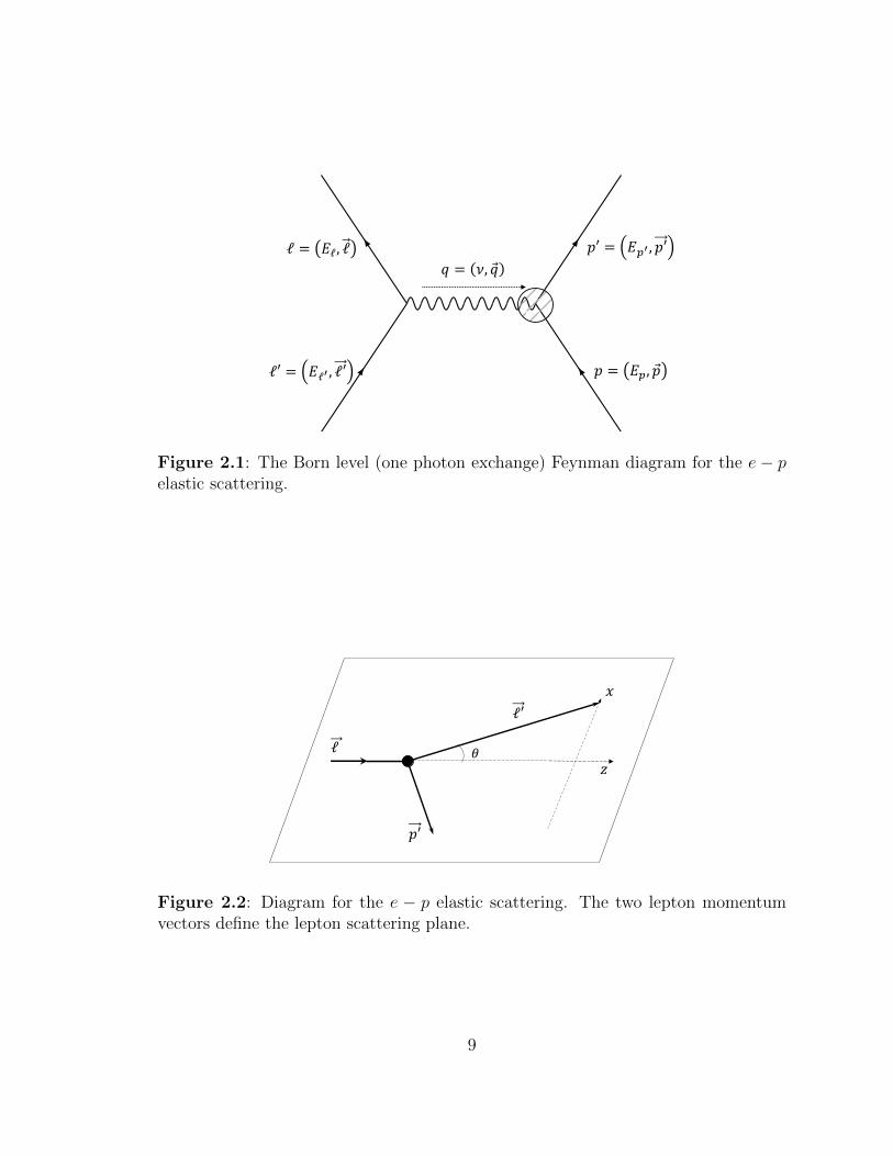
ℓ = #ℓ, ℓ
ℓ′ = #ℓ&, ℓ′ ' = #(, '
'′ = #(&, '′* = +, *
Figure 2.1: The Born level (one photon exchange) Feynman diagram for the e− pelastic scattering.
!
"
ℓ
ℓ′
%
&′
Figure 2.2: Diagram for the e − p elastic scattering. The two lepton momentumvectors define the lepton scattering plane.
9

minus of this quantity squared defines the 4-momentum transfer squared Q2,
Q2 = −q2 = −(`− `′)2 = 2(E`E`′ − ~ · ~′)− 2m2
≈ 4E`E`′ sin2 θ
2= 2E`E`′(1− cos θ),
(2.2)
where the approximation is true if the electron mass (m) squared is negligible. In
the case of elastic scattering, the Q2 can also be expressed as
Q2 = 2Mν = 2M(E` − E`′), (2.3)
in the lab frame.
For the e− p elastic scattering, the differential cross section in the lab frame can
be expressed as
dσ =1
F
|M|24π2
d3~′
2E`′
d3~p′
2Ep′δ(4)(`+ p− `′ − p′), (2.4)
where F = 4√
(` · p)2 −m2M2 ≈ 4E`M is the incident flux factor (the approximation
is true if the electron mass squared is neglected). M is the invariant amplitude that
contains the physics about the electron-proton interaction. It can be expressed as
M = jµ1
q2Jµ, (2.5)
where jµ (Jµ) is the 4-vector transition current density for the electron (proton),
and the Einstein summation convention is applied. The electron transition current
density can be completely described by Quantum Electrodynamics as
jµ = −e u(`′) γµ u(`) ei(`′−`)·x, (2.6)
where e is the charge of the electron. γµ consists of four 4×4 Dirac γ-matrices. They
10

satisfy the anti-commutation relation:
γµ, γν = γµγν + γνγµ = 2gµν , (2.7)
where gµν is the metric tensor with g00 = 1, g11 = g22 = g33 = −1, and all the other
components are 0. In the Dirac-Pauli representation, these matrices can be expressed
as
γ0 =
I 0
0 −I
, ~γ =
0 ~σ
−~σ 0
, (2.8)
where ~σ are the Pauli matrices:
σ1 =
0 1
1 0
, σ2 =
0 −i
i 0
, σ3 =
1 0
0 −1
, (2.9)
u(`) e−i`·x is the positive-energy solution to the Dirac equation (iγµ∂µ−m)ψ = 0 for
a free particle; u(`) ≡ u(`)†γ0 by definition, and u(`) is a 4-component Dirac spinor:
u(s) =√E +m
χ(s)
~σ·~pE+m
χ(s)
, χ(1) =
1
0
, χ(2) =
0
1
. (2.10)
On the other hand, if the proton is also a structureless particle, its transition
current density can be constructed exactly as in Eq. 2.6, with a positive sign stand-
ing for the positive charge of the proton. However, as we know, the proton is an
extended object, and the most general form of its transition current density, under
11
the requirement of Lorentz invariance and parity conservation, can be written as
Jµ = e u(p′)[F1(q2)γµ +
κ
2MF2(q2)iσµνqν
]u(p) ei(p
′−p)·x, (2.11)
where F1(q2) and F2(q2) are the Dirac and Pauli form factors, respectively. They are
related to the internal structure of the proton. κ is the proton anomalous magnetic
moment and σµν is the antisymmetric tensor:
σµν =i
2[γµ, γν ] =
i
2(γµγν − γνγµ) . (2.12)
Combining with Eq. 2.4 and Eq. 2.5, one can derive the differential cross section for
the e− p elastic scattering in the lab frame:
dσ
dΩ=
(dσ
dΩ
)Mott
×[((F1(q2))2 − κ2q2
4M2(F2(q2))2)− q2
2M2(F1(q2) + κF2(q2))2tan2 θ
2
],
(2.13)
where (dσ/dΩ)Mott is the Mott cross section that describes the scattering off the
structure-less and spin-less proton:
(dσ
dΩ
)Mott
=α2cos2 θ
2
4E2` sin
4 θ2
E`′
E`. (2.14)
It is common to use the Sachs form factors [30], which are linear combinations of
F1(q2) and F2(q2):
GpE(Q2) ≡ F1(q2) +
κq2
4M2F2(q2),
GpM(Q2) ≡ F1(q2) + κF2(q2), (2.15)
12
such that no interference term of the form factors will appear in the cross section,
and Eq. 2.13 can be re-written in a much simpler form:
dσ
dΩ=
(dσ
dΩ
)Mott
1
1 + τ
[(Gp
E(Q2))2 +τ
ε(Gp
M(Q2))2], (2.16)
with τ = Q2/(4M2) and ε = [1 + 2(1 + τ) tan2 (θ/2)]−1. Eq. 2.16 is often referred to
as the Rosenbluth formula [30].
It is worth noticing that in the Q2 → 0 limit, the wavelength of the virtual photon
becomes significantly larger than the size of the proton. Effectively it will “see” the
proton as a point target with charge e and magnetic moment (1 + κ)e/2M . This
requires that F1(0) = 1 and F2(0) = 1, and the Sachs form factors become
GpE(0) = 1,
GpM(0) = 1 + κ = µp. (2.17)
In the case that the electron mass is not neglected, as shown in Ref. [31], the
Rosenbluth formula is still applicable, provided that one uses the following two ex-
pressions for ε and the Mott cross section:
ε =
[1− 2(1 + τ)
2m2 −Q2
4E`E`′ −Q2
]−1
, (2.18)
(dσ
dΩ
)Mott
=α2
4E2`
1−Q2/(4E`E`′)
Q4/(4E`E`′)
E`|~′|E`′|~|
M(E2`′ −m2)
ME`E`′ +m2(E`′ − E` −M). (2.19)
13
!" = (% = 0, ! )* = (+,, * )
*′ = (+,, *′ = −* )
Figure 2.3: The e− p elastic scattering in the Breit frame.
2.2 Proton Form Factors
In the classical literature [29], the proton electric and magnetic form factors are
interpreted as the Fourier transforms of the proton charge and magnetic moment
distributions in the non-relativistic limit:
GpE,M(Q2) =
∫ρpE,M(~x) ei~q·~xd3x. (2.20)
This can be achieved in the Breit frame (or the brick wall frame), as shown in Fig. 2.3.
In this frame, the proton bounces back as if it is hitting a brick wall, after absorbing
the virtual photon. The proton has the same energy and momentum magnitude after
the scattering but the direction is flipped. With the z-axis pointing in the direction
of the incident proton, it is straightforward to write down the following formulae for
the kinematic variables in this frame:
Ep = Ep′ ,
ν = 0,
~p = −~p′ = 1
2~q,
Q2 = |~q|2. (2.21)
14

Assuming the density distributions are spherically symmetric and if one takes the
Taylor expansion at the Q2 → 0 limit, then:
GpE,M(Q2) =
∫ (1 + i~q · ~x− (~q · ~x)2
2+ . . .
)ρpE,M(~x)d3x
= 1− 1
6〈rpE,M
2〉Q2 + . . . (2.22)
The mean square charge and magnetic radii can then be identified as1:
〈rpE2〉 ≡ −6
dGpE(Q2)
dQ2
∣∣∣∣Q2=0
, (2.23)
〈rpM2〉 ≡ − 6
µp
dGpM(Q2)
dQ2
∣∣∣∣Q2=0
. (2.24)
These two quantities are in general close to each other, but do not have to be the
same. The charge radius is related to the charge density distribution, while the
magnetic radius is related to the current density distribution. It would be interesting
to see what lattice QCD calculations [32] will predict for the relationship between
the two in the future.
This Fourier transform interpretation of the form factors (Eq. 2.22) was first
proved by Sachs in 1962 [33]. Note that after using the Gordon decomposition
u(p′)γµu(p) = u(p′)
[(p+ p′)µ
2M+ iσµν
(p′ − p)ν2M
]u(p), (2.25)
to replace the tensor term in Eq. 2.11, it is easy to show that the proton 4-vector
1As the work of this dissertation focuses only on the proton charge radius, we will use rp ≡ rpE forsimplicity.
15

transition current can be written as
Jµ = e u(p′)
[γµ(F1 + κF2)− (p+ p′)µ
2MκF2
]u(p) ei(p
′−p)·x. (2.26)
Using Eq. 2.8 and Eq. 2.10, it is straightforward to show that in the Breit frame, the
proton transition current becomes:
Jµ = 2Meχ′†(GpE(Q2), i
~σ × ~q2M
GpM(Q2)
)χ, (2.27)
where the time-like component GpE(Q2) is clearly related to the charge density of the
proton while GpM(Q2) is related to the space-like components and thus related to the
magnetization density of the proton. To obtain the Fourier transform interpretation
as in Eq. 2.20, one can compute the moments of density distributions and take the
non-relativistic (Q2 → 0) limit, as shown in Appendix II of [33].
In the modern physics context, it is more appropriate to define a two-dimensional
charge density distribution in the transverse space [10]. In fact, a three-dimensional
charge density distribution cannot be defined properly because the longitudinal com-
ponent is clearly frame-dependent due to Lorentz contraction. A transverse charge
density distribution can be defined in the infinite-momentum frame [10]:
ρ(b) ≡∑q
eq
∫dx q(x,~b) =
∫d2q
(2π)2F1(Q2 = ~q 2)e−i~q·
~b, (2.28)
where b is the transverse distance from the z−axis (along the longitudinal direction),
F1 is the Dirac form factor as appeared in Eq. 2.13, and the summation is performed
over all quark flavors. In this case, the mean square charge radius can be determined
as:
〈b2〉 =
∫d2b b2 ρ(b) = −4F ′1(0). (2.29)
16

In other words, the quantity defined in Eq. 2.23 is not strictly related to the second
moment of the three-dimensional proton charge density distribution. In Chapter 1,
we mentioned that the proton charge radius can also be measured using hydrogen
spectroscopy. Thus, it is important to examine whether these two different experi-
mental methods are measuring the same quantity. This consistency is presented in
Ref. [10], which shows that the quantity defined in Eq. 2.23 is indeed responsible for
the shift in the transition frequency of atomic energy levels due to the proton finite
size effect:
∆E = −4παG′pE(0)|ψn0(0)|2δl0
= 4παr2p
6|ψn0(0)|2δl0. (2.30)
where |ψn0(0)| is the electron wave function at the origin in coordinate space and the
term is non-vanishing only for a S-state (l = 0). However, it is worth noticing that in
the spectroscopic case, the measurement is done at Q2 = 0 while for the scattering
experiments, the quantity is accessed through an extrapolation from low Q2 form
factor measurements down to Q2 = 0.
2.3 Proton Form Factors from e− p Scattering Experiments
The cross section for the e − p elastic scattering is shown in Eq. 2.16, which con-
tains the contributions from both the electric and magnetic form factors. In order
to separate them, in principle, one would need to have at least two independent
measurements at the same Q2. Some techniques for the unpolarized e − p elastic
scattering will be introduced in Sub-section 2.3.1, including the most commonly ap-
plied Rosenbluth separation method [34], which requires multiple measurements of
17
the unpolarized cross section at the same Q2. Another method is to use the polarized
e − p elastic scattering, which is sensitive directly to the form factor ratio GpE/G
pM .
In this case, the two form factors can be de-coupled by combining the ratio measure-
ment with the unpolarized cross section measurement. The polarized e − p elastic
scattering will be discussed in Sub-section 2.3.2 and Sub-section 2.3.3.
2.3.1 Unpolarized Measurements
The most commonly applied technique to extract GpE and Gp
M from the unpolarized
e− p elastic scattering cross section is the Rosenbluth separation method [34]. First
of all, one needs to re-write the cross section (Eq. 2.16) into a reduced form
( dσdΩ
)reduced
= (1 + τ)ε
τ
(dσdΩ
)ep(
dσdΩ
)Mott
= (GpM(Q2))2 +
ε
τ(Gp
E(Q2))2, (2.31)
where (dσ/dΩ)ep is the Rosenbluth formula (Eq. 2.16). And then, one can obtain
(GpM)2 and (Gp
E)2/τ from the intersection and slope of a linear fit to the reduced
cross sections at the same Q2 but with different values of ε. This can be achieved
by using different beam energies and scattering angles. An example is presented in
Fig. 2.4 where the data points are normalized by the standard dipole form factor:
GD =1
(1 + Q2
0.71(GeV/c)2)2. (2.32)
Alternatively, one can parameterize GpE and Gp
M with different functions, and then
fit the unpolarized cross section directly to extract the two form factors. Such a
technique was used in the Mainz 2010 analysis [5] and a global analysis work [35].
Lastly, in a very low Q2 region and especially when the scattering angles θ are
small, the cross section is completely dominated by the electric form factor. This
18

Figure 2.4: An example demonstrating the Rosenbluth separation technique. Datapoints are shown for the Q2 values of 2.5 (open triangles), 5.0 (open circles) and 7.0(filled triangles) (GeV/c)2. The straight lines are linear fits to the corresponding datapoints. The figure is obtained from Ref. [34].
19
is due to the kinematic factor τ/ε in front of the magnetic form factor. One can
extract GpE alone assuming Gp
M follows certain models or parameterizations, with an
associated systematic uncertainty taken into account. This approach was adopted in
the analysis of Simon [36], in which a simple scaling relation
GpE =
GpM
µp(2.33)
was assumed. The Q2 coverage of this experiment was from 0.005 to 0.055 (GeV/c)2.
For the PRad experiment, the maximum Q2 is comparable to that of Ref. [36], but
the value for the minimum Q2 is one order of magnitude lower. At the same time, the
scattering angular range (0.7 to 7.0) is very small so that ε is nearly 1 (0.99243 to
0.99993), which is its maximum. One would expect a smaller systematic uncertainty
for the PRad experiment, if a similar approach is applied.
Previous unpolarized e−p elastic scattering experiments were typically done with
the magnetic spectrometer method, in which the spectrometer needed to be shifted
to different angles in order to cover the desired angular or Q2 range. A classical
example of this type of experiment is the Mainz 2010 measurement [5], which took
place at the Mainz Microtron. In this experiment, over 1400 cross section data points
were measured, covering Q2 from 0.004 to 1 (GeV/c)2, with statistical uncertainties
better than 0.2% per point. The experiment used a liquid hydrogen target system,
and three spectrometers, with one of the spectrometers in a fixed position in order
to determine the relative luminosity. The extracted GpE and Gp
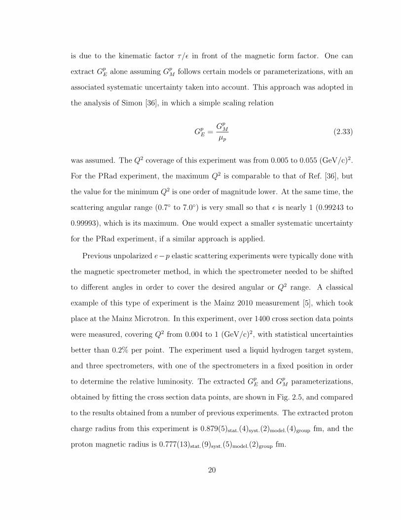
M parameterizations,
obtained by fitting the cross section data points, are shown in Fig. 2.5, and compared
to the results obtained from a number of previous experiments. The extracted proton
charge radius from this experiment is 0.879(5)stat.(4)syst.(2)model.(4)group fm, and the
proton magnetic radius is 0.777(13)stat.(9)syst.(5)model.(2)group fm.
20

0.95
0.96
0.97
0.98
0.99
1
1.01
1.02
1.03
1.04
0 0.05 0.1 0.15 0.2
GE/G
std.
dip
ole
[13][2]Simon et al.Price et al.
Borkowski et al. [15]Janssens et al.Murphy et al. [16]
0.8
0.85
0.9
0.95
1
1.05
0 0.2 0.4 0.6 0.8 1
GE/G
std.
dip
ole
[13][2]Christy et al.Simon et al.Price et al.Berger et al.Hanson et al.
Borkowski et al. [15]Janssens et al.Murphy et al. [16]
0.94
0.96
0.98
1
1.02
1.04
1.06
1.08
1.1
0 0.2 0.4 0.6 0.8 1
GM
/(µ p
Gst
d. d
ipol
e)
[13][2]Christy et al.Price et al.Berger et al.
Hanson et al.Borkowski et al. [15]Janssens et al.Bosted et al.Bartel et al.
0.75
0.8
0.85
0.9
0.95
1
1.05
1.1
0 0.2 0.4 0.6 0.8 1
µ pG
E/G
M
Q2 / (GeV/c)2
[13] w/o TPE[13] w/ TPE[2]Crawford et al.
Gayou et al.Milbrath et al.Punjabi et al.Jones et al.
Pospischil et al.Dieterich et al.Ron et al. [17]
Figure 2.5: The extracted proton GpE and Gp
M parameterizations from the Mainzexperiment [5]. The figures are obtained from Ref. [5].
21

Figure 2.6: The proton electric form factor results from the Saskatoon experiment,obtained by measuring the recoil proton from the elastic e− p scattering. The solidline is a least-squares fit to the data points. The figure is taken from Ref. [37].
Most of the unpolarized e − p cross section measurements, including the Mainz
2010 and the PRad experiments, were done by detecting the scattered electrons.
Equivalently, one can measure the cross section by detecting the recoil proton. In this
case, one would integrate over the electron variables in Eq. 2.4 instead of the proton
variables. One of the major advantages of this approach is that the radiative effects
are significantly smaller for the protons than for the electrons. An experiment of
this kind was performed in Saskatoon, Canada, and the results [37] were published in
1974. The proton electric form factor results, covering Q2 from 5.8×10⁻³ to 3.1×10⁻²
(GeV/c)2, are shown in Fig. 2.6. The scaling relation Eq. 2.33 was assumed in the
extraction. The proton charge radius determined from this experiment is 0.81(3) fm.
22

2.3.2 Polarization Transfer Measurements
Most of -and especially early- proton from factor measurements, were obtained by
measuring the unpolarized e − p elastic scattering cross sections and by using the
Rosenbluth separation method. This method works very well in the kinematic re-
gion where both electric and magnetic form factors contribute to the cross section
significantly. However, due to the kinematic factor τ/ε appearing in front of GpM
(see Eq. 2.16), the electric form factor will dominate the cross section if Q2 and θ
are small, while the magnetic form factor becomes dominant at high Q2 and large
scattering angles. Thus, the electric form factor data obtained in this way typically
have large uncertainties in the high Q2 region while the magnetic form factor uncer-
tainties are larger in the low Q2 region. In addition, the Rosenbluth method may be
more sensitive to systematic uncertainties that are beam-energy-dependent. These
difficulties may be overcome by using the polarized e − p elastic scattering, which
allows one to measure directly the form factor ratio GpE/G
pM at a given Q2 point, in
addition to the cross section measurement. One of the techniques is the polarization
transfer measurement. In this case, one uses a longitudinally polarized electron beam
and an unpolarized proton target, and then measures the polarization transferred to
the recoil proton. The form factor ratio can be expressed as [38]
GpE
GpM
= −PtPl
E` + E`′
2Mtan
θ
2, (2.34)
where Pt and Pl are the transverse and longitudinal components of the proton polar-
ization in the lepton scattering plane (defined by the incident and scattered leptons).
One of the very recent measurements using this technique is the Jefferson Lab E08-
007 experiment [38], performed in the experimental Hall A. The experiment was
performed using a 1.2 GeV polarized electron beam and a cryogenic hydrogen target.
23
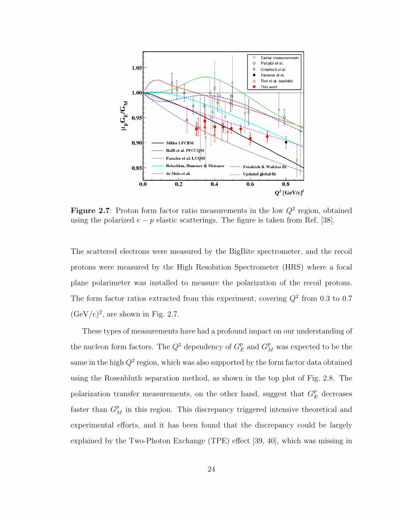
Figure 2.7: Proton form factor ratio measurements in the low Q2 region, obtainedusing the polarized e− p elastic scatterings. The figure is taken from Ref. [38].
The scattered electrons were measured by the BigBite spectrometer, and the recoil
protons were measured by the High Resolution Spectrometer (HRS) where a focal
plane polarimeter was installed to measure the polarization of the recoil protons.
The form factor ratios extracted from this experiment, covering Q2 from 0.3 to 0.7
(GeV/c)2, are shown in Fig. 2.7.
These types of measurements have had a profound impact on our understanding of
the nucleon form factors. The Q2 dependency of GpE and Gp
M was expected to be the
same in the highQ2 region, which was also supported by the form factor data obtained
using the Rosenbluth separation method, as shown in the top plot of Fig. 2.8. The
polarization transfer measurements, on the other hand, suggest that GpE decreases
faster than GpM in this region. This discrepancy triggered intensive theoretical and
experimental efforts, and it has been found that the discrepancy could be largely
explained by the Two-Photon Exchange (TPE) effect [39, 40], which was missing in
24

the earlier analyses using the Rosenbluth separation method. The TPE corrected
form factor ratios from the Rosenbluth separation method are shown in the bottom
plot of Fig. 2.8, and are compared to the polarization transfer measurements.
Individual form factors can be obtained by combining the ratio measurements
with unpolarized cross section measurements. And the proton charge and magnetic
radii can be constrained by the low Q2 ratio measurements. A number of global
analyses of this type are presented in Ref. [13, 35, 38].
2.3.3 Double Polarization Measurements
The proton form factor ratio GpE/G
pM can also be extracted from a double polarization
experiment, with a longitudinally polarized electron beam and a polarized proton
target. In this case, the differential cross section for the e − p elastic scattering can
be expressed as [41]
dσ
dΩ= Σ + h∆, (2.35)
where Σ is the unpolarized differential cross section as shown in Eq. 2.16. h is the
helicity of the incident electron (+1 for positive helicity and -1 for negative helicity),
and ∆ is the spin-dependent differential cross section:
∆ = −(dσ
dΩ
)Mott
f−1recoil[2τvT ′ cos θ∗(Gp
M)2
− 2√
2τ(1 + τ) vTL′ sin θ∗ cosφ∗Gp
MGpE],
(2.36)
where frecoil = 1+2ε sin2 (θ/2)/M, vT ′ =√
1/(1 + τ) + tan (θ/2) tan (θ/2) and vTL′ =
−(1/√
2)/(1 + τ) tan (θ/2). The angles θ∗ and φ∗ are the polar and azimuthal angles
of the proton polarization in the frame with the x− z plane defined by the incoming
and outgoing electrons, and with the z-axis along the direction of the virtual photon,
25

Figure 2.8: Proton form factor ratios obtained using the Rosenbluth separationmethod (red open circles), and polarization transfer measurements (blue solid dia-monds). The Rosenbluth results are shown without (with) the TPE correction in thetop (bottom) plot. The figure is taken from Ref. [35]
26
!
"
ℓ
ℓ′Proton
Polarization
%&∗
(∗
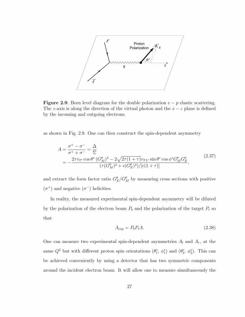
Figure 2.9: Born level diagram for the double polarization e− p elastic scattering.The z-axis is along the direction of the virtual photon and the x− z plane is definedby the incoming and outgoing electrons.
as shown in Fig. 2.9. One can then construct the spin-dependent asymmetry
A =σ+ − σ−
σ+ + σ−=
∆
Σ
= −2τvT ′ cos θ∗ (Gp
M)2 − 2√
2τ(1 + τ)vTL′ sin θ∗ cosφ∗Gp
MGpE
(τ(GpM)2 + ε(Gp
E)2)/[ε(1 + τ)],
(2.37)
and extract the form factor ratio GpE/G
pM by measuring cross sections with positive
(σ+) and negative (σ−) helicities.
In reality, the measured experimental spin-dependent asymmetry will be diluted
by the polarization of the electron beam Pb and the polarization of the target Pt so
that
Aexp = PbPtA. (2.38)
One can measure two experimental spin-dependent asymmetries Al and Ar, at the
same Q2 but with different proton spin orientations (θ∗1, φ∗1) and (θ∗2, φ∗2). This can
be achieved conveniently by using a detector that has two symmetric components
around the incident electron beam. It will allow one to measure simultaneously the
27

two asymmetries with the same target proton spin orientation in the lab frame. And
then, one can extract the form factor ratio and the product of the two polariza-
tions simultaneously. Or one can take the super ratio between the two experimental
asymmetries in order to cancel out the polarizations [2], so that
R =AlAr
=2τvT ′ cos θ∗1 (Gp
M)2 − 2√
2τ(1 + τ)vTL′ sin θ∗1 cosφ∗1G
pMG
pE
2τvT ′ cos θ∗2 (GpM)2 − 2
√2τ(1 + τ)vTL′ sin θ∗2 cosφ∗2G
pMG
pE
. (2.39)
The proton electric and magnetic factors can be de-coupled by combining the form
factor ratio measurements with unpolarized e − p elastic scattering cross section
measurements, similar to the polarization transfer experiments.
This double polarization technique was pioneered by the Bates Large Acceptance
Spectrometer Toroid (BLAST) experiment at MIT-Bates [42], which measured the
form factor ratio from 0.15 to 0.65 (GeV/c)2. The experiment utilized the BLAST
detector [43] (Fig. 2.10), which was equipped with an eight-sector, toroidal, magnetic
field. The two horizontal sectors had detector components installed, which were
symmetric around the beam and simultaneously measured the two experimental spin-
dependent asymmetries, Al and Ar. The experiment also used a windowless target
tube that could be fed with polarized protons produced from either an Atomic Beam
Source or a Laser Driven Source. The extracted proton form factor ratios from this
experiment are shown in Fig. 2.10. The individual form factor can be extracted by
combining the ratio measurements with unpolarized e−p cross section measurements.
Fig 2.11 shows the improvement on GpE and Gp
M due to the BLAST form factor
ratio measurements, when combining with world unpolarized e − p cross section
measurements [44, 45, 46, 47, 48, 49, 50, 51, 52]. This technique will be used in an
experiment at the Mainz Energy-Recovering Superconducting Accelerator (MESA),
which will measure the ratio down to Q2 = 0.005(GeV/c)2 [53].
28

Figure 2.10: Top plot: Main detector components for the BLAST detector. The fig-ure is taken from Ref. [43]. Bottom plot: Proton form factor ratio Gp
E/GpM extracted
from the BLAST experiment at MIT. The figure is taken from Ref.[42].
29

Figure 2.11: Compilation of the GpE/GD (top plot) and Gp
M/(µpGD) at BLASTkinematics with (red square) and without (blue dot) BLAST form factor ratio mea-surements. The figures are taken from Ref. [42].
30

2.4 Hydrogen Sepctroscopy
The proton charge radius can also be extracted from hydrogen spectroscopic experi-
ments, in which the transition frequency between two different hydrogen energy levels
is measured and the proton charge radius is extracted based on high precision bound-
state QED calculations. In the non-relativistic limit and considering the proton to
be infinitely heavy, the time-independent Schrodinger equation is
[− ~p
2
2m+ V
]ψ(~r) = Eψ(~r), (2.40)
where V = −Zα/r is the Coulomb potential of a point-like nucleus with charge Z
(Z = 1 for a hydrogen atom), m is the mass of the electron and α is the fine structure
constant. The energy levels can be obtained by solving the Schrodinger equation
En = −m(Zα)2
2n2= −2πR∞
Z2
n2, (2.41)
where n is the principal quantum number, and R∞ = α2m/(4π) is the Rydberg con-
stant. This is the well-known Bohr energy levels. Although the wave functions ob-
tained with this model depend also on the orbital angular momentum l = 0, 1, . . . , n−
1 and the projection of the orbital angular momentum mz = 0,±1, . . . ,±l, all energy
levels with the same principal quantum number share the same energy. The finite
nuclear mass correction can be easily achieved by replacing the electron mass with
the reduced mass of the system: mr = mM/(m + M), where M is the mass of the
nucleus.
Considering the relativistic energy dependency and the electron spin, a better
description for the hydrogen energy levels can be obtained from the Dirac equation.
31

In the case of an infinitely heavy proton, the energy levels can be expressed as [3, 54],
Enj = mf(n, j), (2.42)
where j = 1/2, 3/2, . . . n− 1/2, is the total angular momentum and
f(n, j) =
1 +(Zα)2(√(
j + 12
)2 − (Zα)2 + n− j − 12
)2
− 1
2
. (2.43)
Notice that in this case, the degeneracy is lifted by the total angular momentum.
However, the energy levels with the same n and j but different l = j ± 1/2 remain
degenerate, such as the 2S1/2 and 2P1/2 states. For the Dirac energy levels, the finite
nuclear mass correction can not be achieved by simply replacing the electron mass
with the reduced mass of the system. Instead, a leading relativistic correction with
an exact mass dependency can be obtained, up to the (Zα)4 order, with an effective
Hamiltonian [3],
H = H0 + VBr, (2.44)
where H0 is the non-relativistic Hamiltonian
H0 =~p 2
2m+
~p 2
2M− Zα
r, (2.45)
and VBr is the Breit potential
VBr =πZα
2
(1
m2+
1
M2
)δ3(~r)− Zα
2mMr
(~p 2 +
~r(~r · ~p) · ~pr2
)+Zα
r3
(1
4m2+
1
2mM
)[~r × ~p ] · ~σ.
(2.46)
32

The result for the energy level is presented in Ref. [3, 55]:
Enjl =(m+M) +mr[f(n, j)− 1]− m2r
2(m+M)[f(n, j)− 1]2
+(Zα)4m3
r
2n3M2
(1
j + 12
− 1
l + 12
)(1− δl0),
(2.47)
where the first two terms are the rest masses, the third term takes into account
the reduced mass effect of the system, and the last two terms are recoil corrections.
Notice that the degeneracy in the Dirac energy levels, with the same n and j but
different l = j ± 1/2, is lifted by the last term in the expression.
The transition frequency between 2S1/2 and 2P1/2 states of a hydrogen atom was
measured by Willis Lamb and Robert Retherford in 1947 [56]. The 2S1/2 state was
found to be higher than the 2P1/2 state by 1 GHz. This difference is certainly not pre-
dicted by the Dirac energy level (Eq. 2.42) and it is still too large for the l-dependent
term in Eq. 2.47, which contributes about 2 kHz to the transition frequency. This
discrepancy was first explained by Bethe in the same year [57]. The main contribu-
tion to this shift is the electron self-energy radiative correction, by emitting and then
absorbing a virtual photon. This effect will smear out the position of the electron
over a certain range and its charge distribution is spread out instead of being a point
charge. This effect shifts the 2S1/2 energy level more than the 2P1/2 as the electron
is much closer to the proton in the former case. Generally speaking, the Lamb shift
includes all the contributions to the energy level, beyond the first three terms in
Eq. 2.47 and without considering the hyperfine splitting. There are four major items
considered in the Lamb shift [54]. Listing with a decreasing order on the contribution,
they include radiative corrections (such as the self-energy and vacuum polarization),
recoil corrections (due to the finite nuclear mass), radiative-recoil corrections (mixed
terms between radiative and recoil corrections) and the finite nuclear size correction.
33

For a hydrogen atom and in the non-relativistic case, the leading order contribution
due to the proton finite size effect is given by Eq. 2.30. This proton finite size effect
originates from the slope of the proton electric form factor at Q2 = 0. For a muonic
hydrogen atom, the proton size contributes to roughly 2% of the Lamb shift [1] be-
tween the 2S1/2 and 2P1/2 energy levels, while for an ordinary hydrogen atom, the
contribution is only about 0.014% [54].
The basic strategy of a hydrogen spectroscopic measurement for the proton charge
radius involves measuring the transition frequency between two different energy lev-
els. The proton charge radius is extracted with all the other terms calculated within
the framework of QED. Generally speaking, there will be two unknowns for a tran-
sition frequency. One is the proton charge radius, and the other one is the Rydberg
constant R∞. There are two types of spectroscopic measurements [9]. One is the
small splitting measurement, which measures the transition frequency between two
states that have the same principal quantum number n. In addition, the proton finite
size effect is only significant if the S-state is involved, for example, the 2S-2P transi-
tion. In this case, the main contributions to the transition frequency are cancelled as
the two states share the same principal quantum number, and the Rydberg constant
is known precisely enough from external measurements. Recent experiments of this
type include the two muonic hydrogen Lamb shift measurements (2SF=11/2 - 2PF=2
3/2 and
2SF=01/2 - 2PF=1
3/2 ) [1, 6], and the 2019 ordinary hydrogen Lamb shift measurement [20]
(2SF=01/2 - 2PF=1
1/2 ). The other type of spectroscopic measurements is the large splitting
measurement, which measures the transition frequency between two states with dif-
ferent principal quantum numbers. In this case, the contribution due to the proton
finite size effect is much smaller relatively and the Rydberg constant is not known
precisely enough. The solution is to measure two transition frequencies at the same
time and then solve for both rp and R∞ with two equations. In fact, the high pre-
34

cision Rydberg constant is determined from these types of measurements, and thus
it is highly correlated with the proton charge radius. Typically, the 1S-2S transition
is measured as one of the equations, as the transition frequency can be determined
very precisely. And again the other transition will have an S-state involved in order
to include the proton finite size effect. The 2017 [18] and 2018 [19] hydrogen spec-
troscopy results were both obtained from experiments of this type. They measured
the transition frequencies between the 2S-4P and 1S-3S states, respectively.
The most precise measurements of the proton charge radius were obtained with
the muonic hydrogen Lamb shift measurements [1, 6], performed at the Paul Scherrer
Institute. Since the muon is about 200 times heavier than the electron, they orbit
about 200 times closer to the proton and are more sensitive to the proton finite size
effect. First of all, these experiments had a low energy muon beam injected into the
target hydrogen gas in order to form muonic hydrogen. 99% of the muonic hydrogen
atoms would de-excit almost immediately to the ground state, with only 1% of them
de-exciting to the meta-stable 2S state (life time about 1 µs), and these were the
events of interest (see A in Fig. 2.12). A laser with tunable frequency was then used
to drive the muons from the 2S state towards the 2P state. Once the muons reached
the 2P state, they would de-excit immediately to the ground state, emitting a 1.9 keV
Kα X-ray (see B in Fig. 2.12), which was measured in coincidence with the incident
laser pulse and the electron from the muon decay (µ− → e−νµνe). The measured
frequency for 2SF=11/2 - 2PF=2
3/2 transition is shown in Fig 2.13 from the 2010 Lamb shift
experiment [1].
35
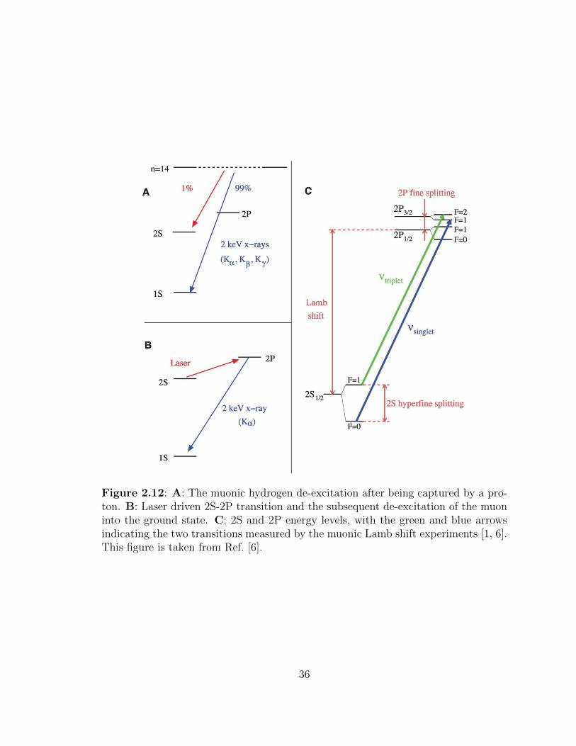
Figure 2.12: A: The muonic hydrogen de-excitation after being captured by a pro-ton. B: Laser driven 2S-2P transition and the subsequent de-excitation of the muoninto the ground state. C: 2S and 2P energy levels, with the green and blue arrowsindicating the two transitions measured by the muonic Lamb shift experiments [1, 6].This figure is taken from Ref. [6].
36

Figure 2.13: The measured frequency for 2SF=11/2 - 2PF=2
3/2 transition of a muonic
hydrogen atom. The figure is taken from Ref. [1].
37
Chapter 3
The Experiment
3.1 Overview
The PRad experiment (E12-11-106) [28] was performed in 2016 in Hall B at Jefferson
Lab, with both 1.1 and 2.2 GeV unpolarized electron beams on a windowless H2 gas-
flow target. The experiment measured the elastic e − p scattering cross section and
the proton electric form factor GpE in the Q2 range 2.1 × 10⁻⁴ − 0.06 (GeV/c)2.
The luminosity was monitored by simultaneously measuring the Møller scattering
process (e − e scattering), which is a well known QED process. The absolute e − p
elastic scattering cross section was normalized to that of the Møller scattering in
order to cancel out the luminosity. The PRad experimental apparatus is shown in
Fig. 3.1. This experiment used a hybrid electromagnetic calorimeter (HyCal) to
detect both the energies and scattering angles of the electrons from both elastic e−p
and e − e scatterings. Their scattering angle measurements were further improved
by two Gas Electron Multiplier (GEM) detectors that were placed side by side in
front of the HyCal. These detectors provided a scattering angular coverage from
0.7 to 7.0 and a full azimuthal angular coverage. To have a better control over the
systematic uncertainties, a 4 cm long, windowless, cryo-cooled H2 gas-flow target was
used in order to remove the majority of the backgrounds generated from the target
cell windows. This target cell was placed inside a target chamber, which was equipped
with multiple turbo pumps in order to maintain a low pressure along the beam-line.
A 5 m long, two-stage vacuum chamber was connected to the target chamber in
38
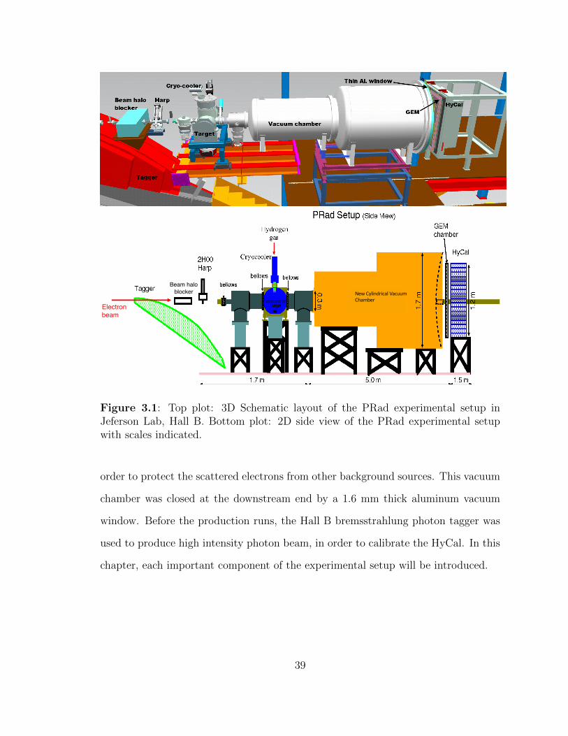
New Cylindrical Vacuum Chamber
Electron beam
Beam halo blocker
Figure 3.1: Top plot: 3D Schematic layout of the PRad experimental setup inJeferson Lab, Hall B. Bottom plot: 2D side view of the PRad experimental setupwith scales indicated.
order to protect the scattered electrons from other background sources. This vacuum
chamber was closed at the downstream end by a 1.6 mm thick aluminum vacuum
window. Before the production runs, the Hall B bremsstrahlung photon tagger was
used to produce high intensity photon beam, in order to calibrate the HyCal. In this
chapter, each important component of the experimental setup will be introduced.
39

Data set Beam energy (MeV) Uncertainty (MeV)1.1 GeV 1101.0 0.52.2 GeV 2143.0 1.5
Table 3.1: Central values and uncertainties of the beam energies for the 1.1 and2.2 GeV data sets.
3.2 The electron beam
The electron beam of the experiment was provided by the Continuous Electron Beam
Accelerator Facility (CEBAF) at Jefferson Lab. There are in total 4 experimental
halls in this facility and the PRad experiment was performed in Hall B. This exper-
iment was one of the first experiments to run after the accelerator upgraded from
6 GeV to 12 GeV beam energy [58]. CEBAF is a recirculating linear accelerator, as
shown in Fig. 3.2. It consists of two linear sections that are connected by two recir-
culating arcs. Each linear section contains multiple cyromodules that can provide in
total about 1.1 GeV energy to the beam energy. The recirculating arcs contain sep-
arated beam lines that are equipped with different dipole and quadrupole magnets.
They can recirculate the electron beam back to the linear section for a maximum of 5
times. This will provide a maximum 11 GeV electron beam to Hall A, B and C. The
electron beam can be accelerated one more time in the north linear section, delivering
a maximum 12 GeV electron beam to Hall D. The electron beam consists of small
bunches that are separated by either 2 ns or 4 ns. The bunch length is typically less
than 100 microns in distance [59].
Two different beam energies were used in this experiment. Table 3.1 shows the
central values and the associated uncertainties from the offline analysis1. The energy
1The nominal beam energy for the second pass beam from the JLab linear accelerator should bearound 2.2 GeV. The actual beam energy 2143 MeV determined later on was slightly less thanthe requested value of this experiment, but we will still use the 2.2 GeV as a label for the dataset taken with the second pass beam, with the understanding that the actual beam energy wasslightly lower.
40

Add arc
Add 5 cryomodules
Add 5 cryomodules
20 cryomodules
20 cryomodules
Upgrade arc magnets and supplies
CHL upgrade
Figure 3.2: An overview of CEBAF at Jefferson Lab.
spread of the electron beam was at the level of 3 × 10⁻⁵, which was significantly
smaller than the uncertainty in the central value. The beam position and beam
current were monitored continuously during the experiment by Hall B beam position
monitors (BPM). In order to study the associated systematic uncertainties, various
beam currents were used during the data taking. For the 1.1 GeV data set, the
majority of runs were taken with 15 nA while others were taken with 10 nA. For
the 2.2 GeV data set, the designated beam current was 55 nA, with several reference
runs at 15 nA, 25 nA and 40 nA. The beam profile was also measured multiple times
in a data taking period, by various harps in Hall B. An example of the harp scan is
shown in Fig. 3.3. The typical profile could be reasonably well described by Gaussian
distributions, with their widths at the level of 20 µm.
41

Figure 3.3: Example of the beam profile measured by harps during the PRad ex-periment.
42
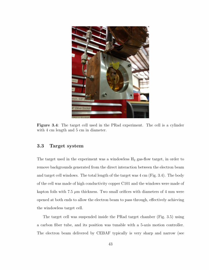
Figure 3.4: The target cell used in the PRad experiment. The cell is a cylinderwith 4 cm length and 5 cm in diameter.
3.3 Target system
The target used in the experiment was a windowless H2 gas-flow target, in order to
remove backgrounds generated from the direct interaction between the electron beam
and target cell windows. The total length of the target was 4 cm (Fig. 3.4). The body
of the cell was made of high conductivity copper C101 and the windows were made of
kapton foils with 7.5 µm thickness. Two small orifices with diameters of 4 mm were
opened at both ends to allow the electron beam to pass through, effectively achieving
the windowless target cell.
The target cell was suspended inside the PRad target chamber (Fig. 3.5) using
a carbon fiber tube, and its position was tunable with a 5-axis motion controller.
The electron beam delivered by CEBAF typically is very sharp and narrow (see
43

Fig. 3.3) but may be accompanied by a long tail that is much wider but lower in its
intensity (beam halo). Thus, the lateral position of the target cell was fine-tuned at
the beginning of each data taking period to align the target cell with the electron
beam so that the main beam could pass the orifices, and to minimize the background
generated from the beam halo hitting the kapton foils. For full target runs, the H2
target gas was cooled to approximately 20 K with a Cryomech pulse tube refrigerator
PT810, prior to be filled inside the cell at a rate of 600 sccm. This was the first time
that a gas-flow target was used on an external beam-line at CEBAF. Due to the
fact that the gas was flowing out of the cell from both orifices, and the importance
to maintain a low background pressure inside the target chamber and the beam-line
vacuum, we needed to pump away the gas flowing into the target chamber from the
target cell. Thus, the target chamber was connected to three Pfeiffer 3200 turbo
pumps and fore pumps to remove leaking H2 gas from the orifices. The chamber
was also connected to an upstream and a downstream chamber. Each of them was
connected to a Pfeiffer 1500 turbo pump and a fore pump in order to maintain low
pressure along the beam-line. With the understanding that the H2 gas inside the
target chamber could be a background source that contaminates the measurement,
empty target runs were taken every few hours. The purpose was to subtract this
background H2 gas contribution, together with contributions from other beam-line
objects like the beam halo blocker (see Fig. 3.1) and target cell windows. For these
empty target runs, the H2 gas was filled in at the same flow rate directly into the
target chamber through a second inlet, in order to mimic the residual gas distribution
far away from the target cell. All the other conditions remained the same as for the
full target runs, for which the second inlet was valved off during the data taking.
More related details will be presented in Section 4.5.1.
Various pressure gauges were used during the experiment to continuously measure
44
Figure 3.5: 3D view of the PRad target system.
the pressure at different locations of the target system. For full target runs when H2
target gas was filled inside the cell, the cell pressure was measured to be about
480 mTorr, which achieved approximately an areal density of 2× 10¹⁸ H atoms/cm2.
The pressure of the target chamber was measured to be about 2.5 mTorr while the
pressure for the rest of the beamline was kept below 0.1 mTorr. For empty target
runs, the measured target chamber pressure was about 2.9 mTorr.
A 5 m long, two-stage vacuum chamber was connected to the target downstream
chamber in order to protect the scattered electrons from other background sources.
This vacuum chamber was closed at the downstream end by a 1.6 mm thick aluminum
vacuum window, immediately in front of the GEM detectors.
45
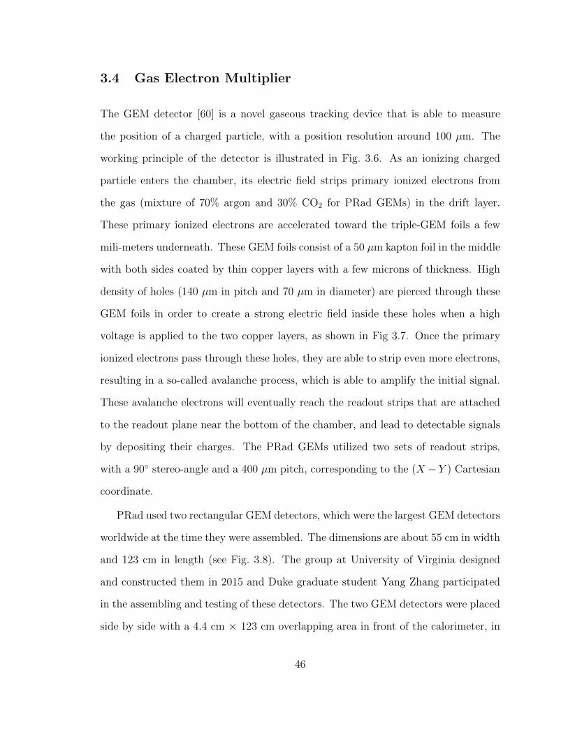
3.4 Gas Electron Multiplier
The GEM detector [60] is a novel gaseous tracking device that is able to measure
the position of a charged particle, with a position resolution around 100 µm. The
working principle of the detector is illustrated in Fig. 3.6. As an ionizing charged
particle enters the chamber, its electric field strips primary ionized electrons from
the gas (mixture of 70% argon and 30% CO2 for PRad GEMs) in the drift layer.
These primary ionized electrons are accelerated toward the triple-GEM foils a few
mili-meters underneath. These GEM foils consist of a 50 µm kapton foil in the middle
with both sides coated by thin copper layers with a few microns of thickness. High
density of holes (140 µm in pitch and 70 µm in diameter) are pierced through these
GEM foils in order to create a strong electric field inside these holes when a high
voltage is applied to the two copper layers, as shown in Fig 3.7. Once the primary
ionized electrons pass through these holes, they are able to strip even more electrons,
resulting in a so-called avalanche process, which is able to amplify the initial signal.
These avalanche electrons will eventually reach the readout strips that are attached
to the readout plane near the bottom of the chamber, and lead to detectable signals
by depositing their charges. The PRad GEMs utilized two sets of readout strips,
with a 90 stereo-angle and a 400 µm pitch, corresponding to the (X − Y ) Cartesian
coordinate.
PRad used two rectangular GEM detectors, which were the largest GEM detectors
worldwide at the time they were assembled. The dimensions are about 55 cm in width
and 123 cm in length (see Fig. 3.8). The group at University of Virginia designed
and constructed them in 2015 and Duke graduate student Yang Zhang participated
in the assembling and testing of these detectors. The two GEM detectors were placed
side by side with a 4.4 cm × 123 cm overlapping area in front of the calorimeter, in
46

0 0 00 0 00 0 00 0 00 0 00 0 0
1 1 11 1 11 1 11 1 11 1 11 1 1
0 0 00 0 00 0 00 0 00 0 00 0 0
1 1 11 1 11 1 11 1 11 1 11 1 1
0 0 00 0 00 0 00 0 00 0 00 0 0
1 1 11 1 11 1 11 1 11 1 11 1 1
0 0 00 0 00 0 00 0 00 0 00 0 0
1 1 11 1 11 1 11 1 11 1 11 1 1
0 0 00 0 00 0 00 0 00 0 00 0 0
1 1 11 1 11 1 11 1 11 1 11 1 1
0 0 00 0 00 0 00 0 00 0 00 0 0
1 1 11 1 11 1 11 1 11 1 11 1 1
0 0 00 0 00 0 00 0 00 0 00 0 0
1 1 11 1 11 1 11 1 11 1 11 1 1
0 0 00 0 00 0 00 0 00 0 00 0 0
1 1 11 1 11 1 11 1 11 1 11 1 1
0 0 00 0 00 0 00 0 00 0 00 0 0
1 1 11 1 11 1 11 1 11 1 11 1 1
0 0 00 0 00 0 00 0 00 0 0
1 1 11 1 11 1 11 1 11 1 1
0 0 00 0 00 0 00 0 00 0 0
1 1 11 1 11 1 11 1 11 1 1
0 0 00 0 00 0 00 0 00 0 0
1 1 11 1 11 1 11 1 11 1 1
0 0 00 0 00 0 00 0 00 0 0
1 1 11 1 11 1 11 1 11 1 1
0 0 00 0 00 0 00 0 00 0 0
1 1 11 1 11 1 11 1 11 1 1
0 0 00 0 00 0 00 0 00 0 0
1 1 11 1 11 1 11 1 11 1 1
0 0 00 0 00 0 00 0 00 0 0
1 1 11 1 11 1 11 1 11 1 1
0 0 00 0 00 0 00 0 00 0 0
1 1 11 1 11 1 11 1 11 1 1
0 0 00 0 00 0 00 0 00 0 0
1 1 11 1 11 1 11 1 11 1 1
0 0 00 0 00 0 00 0 00 0 0
1 1 11 1 11 1 11 1 11 1 1
0 0 00 0 00 0 00 0 00 0 0
1 1 11 1 11 1 11 1 11 1 1
0 0 00 0 00 0 00 0 00 0 0
1 1 11 1 11 1 11 1 11 1 1
0 0 00 0 00 0 00 0 00 0 0
1 1 11 1 11 1 11 1 11 1 1
0 0 00 0 00 0 00 0 00 0 0
1 1 11 1 11 1 11 1 11 1 1
0 0 00 0 00 0 00 0 00 0 0
1 1 11 1 11 1 11 1 11 1 1
0 0 00 0 00 0 00 0 00 0 0
1 1 11 1 11 1 11 1 11 1 1
0 0 00 0 00 0 00 0 00 0 0
1 1 11 1 11 1 11 1 11 1 1
0 0 00 0 00 0 00 0 00 0 0
1 1 11 1 11 1 11 1 11 1 1
0 0 0 0 0 0 0 0 0 0 0 0 0 0 0 0 0 0 0 0 0 0 0 0 0 0 0 0 0 00 0 0 0 0 0 0 0 0 0 0 0 0 0 0 0 0 0 0 0 0 0 0 0 0 0 0 0 0 00 0 0 0 0 0 0 0 0 0 0 0 0 0 0 0 0 0 0 0 0 0 0 0 0 0 0 0 0 00 0 0 0 0 0 0 0 0 0 0 0 0 0 0 0 0 0 0 0 0 0 0 0 0 0 0 0 0 0
1 1 1 1 1 1 1 1 1 1 1 1 1 1 1 1 1 1 1 1 1 1 1 1 1 1 1 1 1 11 1 1 1 1 1 1 1 1 1 1 1 1 1 1 1 1 1 1 1 1 1 1 1 1 1 1 1 1 11 1 1 1 1 1 1 1 1 1 1 1 1 1 1 1 1 1 1 1 1 1 1 1 1 1 1 1 1 11 1 1 1 1 1 1 1 1 1 1 1 1 1 1 1 1 1 1 1 1 1 1 1 1 1 1 1 1 1
0 0 0 0 0 0 0 0 0 0 0 0 0 0 0 0 0 0 0 0 0 0 0 0 0 0 0 0 0 00 0 0 0 0 0 0 0 0 0 0 0 0 0 0 0 0 0 0 0 0 0 0 0 0 0 0 0 0 00 0 0 0 0 0 0 0 0 0 0 0 0 0 0 0 0 0 0 0 0 0 0 0 0 0 0 0 0 0
1 1 1 1 1 1 1 1 1 1 1 1 1 1 1 1 1 1 1 1 1 1 1 1 1 1 1 1 1 11 1 1 1 1 1 1 1 1 1 1 1 1 1 1 1 1 1 1 1 1 1 1 1 1 1 1 1 1 11 1 1 1 1 1 1 1 1 1 1 1 1 1 1 1 1 1 1 1 1 1 1 1 1 1 1 1 1 1
Ionizing Particle
Drift Cathode
GEM foil
GEM foil
GEM foil
Readout Plane
3 mm − Drift
2 mm − Transfer
2 mm − Transfer
2 mm − Induction
−V
Figure 3.6: Working principle of GEM. The figure is taken from [61]
Figure 3.7: The electric field produced by a GEM foil. The figure is taken from[60]
47

Figure 3.8: PRad GEM detectors in the Experimental Equipment Lab at JLab.
order to fully cover its detection region. Each GEM detector had a 4.4 cm × 4.4 cm
hole located at the center of one of the edges to allow the beam pipe to go through.
To prevent GEM foils from direct contact with each other, multiple dielectric
spacers were placed in between them. These spacers are about 3 mm in thickness
and their locations are indicated in Fig. 3.9 as the black solid lines. They can cause
about 3% loss of detection efficiency for PRad GEMs. Each GEM foil was sub-
divided into 60 high voltage sectors, separated by 100 µm gaps. These gaps may also
cause inefficiencies for the GEMs but the effect is significantly smaller compared to
that from the spacers. This effect is shown in Fig. 3.10, where the hit positions of
e − p elastic scattering events on GEMs are shown along one of the readout strip
directions. The large spikes (as indicated in the plot) are due to the GEM spacers,
the much smaller spikes are due to the gaps between the high voltage sectors. The
48

SolidWorks Student Edition. For Academic Use Only.
Figure 3.9: Design for the PRad GEM detector. Black solid lines indicate thelocation of the spacers. The plot is made by Xinzhan Bai of University of Virginia.
GEM efficiency losses due to these spacers and gaps between high voltage sectors
were measured using the data and modeled in the simulation.
The position resolutions of these GEM detectors are typically at the level of
100 µm. For PRad GEMs, the resolution is about 72 µm, which is at least 20 times
better than the position resolution of HyCal. A detected particle by the calorime-
ter will eventually have its reconstructed position replaced by that from the GEM
detectors. Thus, they are able to significantly improve the scattering angle and Q2
resolution of the PRad setup.
3.5 Hybrid Calorimeter
The calorimeter used in this experiment is a hybrid electromagnetic calorimeter [62],
constructed by the PrimEx collaboration [63] and Jefferson Lab, and used during the
PrimEx-I and PrimEx-II experiments [64, 65]. It consists of 1152 PbWO4 modules
49
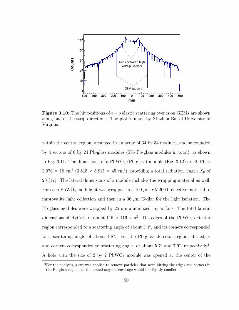
500- 400- 300- 200- 100- 0 100 200 300 400 500mm
1
10
210
310
410
510
Counts
GEM spacers
Gaps between high voltage sectors
Figure 3.10: The hit positions of e−p elastic scattering events on GEMs are shownalong one of the strip directions. The plot is made by Xinzhan Bai of University ofVirginia.
within the central region, arranged in an array of 34 by 34 modules, and surrounded
by 4 sectors of 6 by 24 Pb-glass modules (576 Pb-glass modules in total), as shown
in Fig. 3.11. The dimensions of a PbWO4 (Pb-glass) module (Fig. 3.12) are 2.076 ×
2.076 × 18 cm3 (3.815 × 3.815 × 45 cm3), providing a total radiation length X0 of
20 (17). The lateral dimensions of a module includes the wrapping material as well.
For each PbWO4 module, it was wrapped in a 100 µm VM2000 reflective material to
improve its light collection and then in a 36 µm Tedlar for the light isolation. The
Pb-glass modules were wrapped by 25 µm aluminized mylar foils. The total lateral
dimensions of HyCal are about 116 × 116 cm2. The edges of the PbWO4 detector
region corresponded to a scattering angle of about 3.4, and its corners corresponded
to a scattering angle of about 4.8. For the Pb-glass detector region, the edges
and corners corresponded to scattering angles of about 5.7 and 7.9, respectively2.
A hole with the size of 2 by 2 PbWO4 module was opened at the center of the
2For the analysis, a cut was applied to remove particles that were hitting the edges and corners inthe Pb-glass region, so the actual angular coverage would be slightly smaller.
50

Figure 3.11: Front view of the HyCal electromagnetic calorimeter. The photo istaken from [63].
detector to allow the beam pipe to go through. A square shaped tungstate absorber
was located immediately in front of the calorimeter to cover the inner-most layer of
PbWO4 modules (12 modules in total). This absorber would partially block events
with scattering angles from 0.2 to 0.6, in order to protect these PbWO4 modules
from the ultra-high event rates.
This detector is excellent in detecting and measuring the energy of electrons and
photons. As these particles enter HyCal modules, they will initiate electromagnetic
showers that are cascades of secondary particles including electrons, positrons and
photons, with less and less energy as the showers develop. Even though both PbWO4
and Pb-glass are electromagnetic calorimeters, their working principles are slightly
different. PbWO4 is a scintillating type of calorimeter, for which charged particles
in the shower produce fluorescence light through the ionization process, while Pb-
glass is a Cherenkov type of calorimeter, for which the light is produced by the
51

Figure 3.12: PbWO4 (small) and Pb-glass (large) modules of HyCal calorimeter.The photo is taken from [63].
Cherenkov process of the charged particles in the shower [66]. In both cases, the
produced photons are collected by a photon multiplier tube (PMT) attached to the
back of each module, and the size of the signal is approximately proportional to the
energy of the initial incident electron and photon. The proportionality constants
(calibration constants) can be obtained, if one calibrates the detected signal from the
PMTs to the energy of the incident particle, which needs to be determined by some
additional sources. These constants may depend on various variables, such as the
light attenuation property of the module, the high voltage applied to the PMT and
so on.
Since calibration constants are usually determined at some specific times (calibra-
tion runs for instance) while their dependent variables may not be constant during the
entire experiment, it is necessary to have a particular system to monitor the possible
shifts for these constants. For this purpose, a light monitoring system (LMS) [67]
was adopted, based on a pulsed nitrogen laser. The light produced was delivered to
all HyCal modules by optical fibers that were attached to their front ends, as shown
52

Figure 3.13: Front view of HyCal. Each module has a LMS optical fiber attachedto its front end (1728 modules in total). The photo is taken from [63]
in Fig. 3.13. In addition, the light produced by the same source was delivered to
three additional PMTs (reference PMTs), which also had 241Am radioactive sources
and scintillators attached. The main decay channel of 241Am is α-decay, by emitting
an α particle and a photon that are almost at constant energies. This setup allows
one to calculate a gain correction factor, which can change as a function of time (t)
g(t) =ALMSi × Aαref
ALMSref
, (3.1)
where ALMSi is the signal amplitude of the i-th HyCal module due to the LMS light
source, Aαref is the signal amplitude of a reference PMT due to the 241Am radioactive
source and ALMSref is the signal amplitude of the same reference PMT due to the LMS
light source. To correct for a calibration constant, one can multiply it by the factor
g(tf )/g(t0), where g(tf ) is the current gain correction factor and g(t0) is the gain
correction factor when the calibration constant was obtained.
53
For the PRad experiment, HyCal served as the main detector for two major
purposes. First, the measured energy of the scattered electron was used for the event
selection, which means to select e− p and e− e elastic scattering events and to reject
backgrounds. Second, the total energy deposition in HyCal was used for triggering the
data acquisition system (DAQ) during the production runs (the full target runs and
the empty target runs). Because the performance of Pb-glass modules was expected
to be better at a slightly higher energy than that of this experiment, the total energy
deposition in Pb-glass modules was solely utilized as an additional trigger with a
lower threshold.
3.6 Hall B Photon Tagger
The bremsstrahlung photon tagger [68] in Hall B at Jefferson Lab was used to cali-
brate the HyCal (calibration runs) prior to the data taking of the production runs.
First of all, the electron beam was incident onto a thin wire radiator, and a por-
tion of the electrons would radiate photons through the bremsstrahlung process. As
shown in Fig. 3.14, the electrons would be banded by a dipole magnet placed im-
mediately downstream of the radiator while the radiated photon would move along
the initial electron beam direction and eventually injected into the HyCal. After
the bremsstrahlung radiation, the electrons with different energies will have different
curvatures inside the magnetic field. Their energies and timing information are mea-
sured by 384 partially overlapping E-counters and 61 T-counters, respectively. The
energy of the radiated photon can be determined from the difference between the
electron beam energy and the energy determined by the E-counters,
Eγ = Eb − Ee. (3.2)
54

Figure 3.14: The bremsstrahlung photon tagger in Hall B at Jefferson Lab. TheFigure is taken from Ref. [68]
This photon tagger is capable of measuring the energy of the radiated photon from
20% to 95% of the electron beam energy (Eb), up to Eb = 6.1 GeV, and with an energy
resolution of 10−3Eb [68]. The timing resolution of this tagger is about 110 ps [68].
3.7 Triggers and Data Acquisition
This experiment used the CEBAF Online Data Acquisition (CODA) system, which
recorded the data from front-end electronics and wrote into binary data files (evio).
The electronics for HyCal were mostly inherited from the PrimEx experiments [63, 64,
65]. The complete PRad DAQ system for production runs is illustrated by Fig. 3.15.
The signals from the PMTs of HyCal modules were divided into anode and dynode
signals. The anode signals from all 1728 HyCal modules were recorded using 30
ADC1881M modules contained in 3 FastBus crates. The integrated charge within a
280 ns time window from the PMT of each HyCal module was converted into digital
55

signals and written into the data stream. These 1728 modules were grouped into 52
Time-to-Digital Convertor (TDC) groups, with about 36 modules in each group. The
dynode signals from all modules within a TDC group were first summed linearly by
using 52 homemade modules (UVA120A) from University of Virginia. A copy of the
produced signals would be sent to the JLab discriminators located in a VME crate.
They were recorded by the CAEN v1990 TDC modules in the data stream as the
timing information for the TDC groups. Signals from the other copy were summed
using 5 NIM modules into a total sum signal, which was then converted into ECL
signal (see Fig. 3.16) and sent to the Trigger Interface (TI) master located in the same
VME crate. The TI master would then distribute the signal to the TI slaves, which
were synchronized to the TI master. The TI slaves would then send signals to all the
controlled crates for recording the triggered events. In addition to the triggers from
the HyCal, the TI master also received triggers from a pulser of the LMS system of
HyCal, and triggers from the 241Am sources attached on the reference PMTs. These
triggers were used to monitor the gain of the HyCal at the beginning of each run of
the data taking.
The total sum signal was also used to trigger the readout system for the GEM
detectors, which was a APV25 [69] based Scalable Readout System (SRS) [70]. 72
APVs, each with 128 channels, were used to record the data from in total 9216
channels from the two GEM detectors. These APV25s are analogue pipe-line readout
chips, which measure the signal amplitudes from the GEM readout strips every 25 ns
and store the information in a 192-cell analogue pipeline. They were connected,
through HDMI connectors, to ADC boards, which were then connected to the Front-
End Concentrator cards (FEC) located in the SRS crate. These FECs are FPGA
based cards and are capable of managing the outputs from the ADC boards and
receiving the triggers. As multiple FECs were used in the PRad experiment, they
56

Linear Sum
Gate for Fastbus ADCs
Trigger to TI master
Trigger to TI slaves
Timing information to JLab discriminators
Sum
HyCalAnode signals
Dynode signals -> TDC groups
GEMSRS
Crate
Trigger to SRS
SRS data to CPUTrigger from LMS pulserTrigger from 241Am-sources
Figure 3.15: The configuration of the PRad DAQ system for the production runs.This plot is made by Chao Peng of Duke University.
PbWO4
Figure 3.16: Summing all 52 signals from the UVA120A modules, using NIM mod-ules. The final total sum signal is converted into ECL signal in order to be acceptedby the TI master. This plot is made by Chao Peng of Duke University.
57
were connected to a higher level board called Scalable Readout Unit (SRU), which
was connected to the DAQ computer using fibers. The HyCal total sum trigger would
be sent to this DAQ computer, which would forward this signal to a NIM module to
convert it from ECL signal to a NIM signal. This NIM signal would be eventually
sent to the SRU, which would distribute it to the hosted FECs. The output data
consisted of three consecutive samples from each strip in GEMs, measured by the
APV25s, and were transferred to the data stream using a 10 Gb Ethernet.
For the calibration runs, the DAQ configuration was very similar to that of the
production runs, with the exception that the trigger was produced by the Hall B
photon tagger instead of HyCal, and there was an additional data stream to data files,
including the photon energy and timing measured by the tagger. A separated VME
crate (tagger crate) was integrated into the DAQ system, which had an additional
TI master that received the trigger from the tagger and controlled all the TI slaves
shown in Fig. 3.15.
In addition to the data from GEMs and HyCal, the output data also included in-
formation from the Experimental Physics and Industrial Control System (EPICS) and
the scaler events. The EPICS events were taken every few seconds, which included
pressure measurements at various locations along the beam-line, beam positions mea-
sured by various Beam Position Monitors (BPM), the target related gas flow rate,
pressure, temperature, and so on. The scaler events, which were taken every 20 to
50 seconds, contained the information to calculate the dead time of the DAQ system
and the total beam charge. Once the DAQ system received a trigger, it would start
recording the current event, which would take about 20 µs. The system would be in
a “busy mode” and would not be able to response to additional triggers during this
period. This would lead to a “dead time” (tdead) of the system. To measure this, a
pulser with a constant frequency of 2.0 MHz was used and tdead could be calculated
58
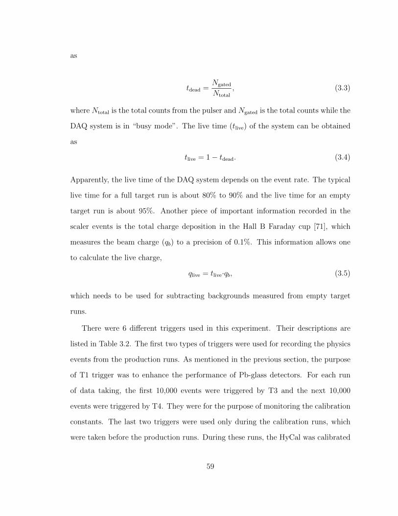
as
tdead =Ngated
Ntotal
, (3.3)
where Ntotal is the total counts from the pulser and Ngated is the total counts while the
DAQ system is in “busy mode”. The live time (tlive) of the system can be obtained
as
tlive = 1− tdead. (3.4)
Apparently, the live time of the DAQ system depends on the event rate. The typical
live time for a full target run is about 80% to 90% and the live time for an empty
target run is about 95%. Another piece of important information recorded in the
scaler events is the total charge deposition in the Hall B Faraday cup [71], which
measures the beam charge (qb) to a precision of 0.1%. This information allows one
to calculate the live charge,
qlive = tlive·qb, (3.5)
which needs to be used for subtracting backgrounds measured from empty target
runs.
There were 6 different triggers used in this experiment. Their descriptions are
listed in Table 3.2. The first two types of triggers were used for recording the physics
events from the production runs. As mentioned in the previous section, the purpose
of T1 trigger was to enhance the performance of Pb-glass detectors. For each run
of data taking, the first 10,000 events were triggered by T3 and the next 10,000
events were triggered by T4. They were for the purpose of monitoring the calibration
constants. The last two triggers were used only during the calibration runs, which
were taken before the production runs. During these runs, the HyCal was calibrated
59
Trigger name DescriptionT1 Total energy deposition in Pb-glass part of HyCalT2 Total energy deposition in HyCalT3 LMS light sourceT4 241Am radioactive sourceT5 Hall B tagger counterT6 Scintillator
Table 3.2: PRad trigger type description.
by high intensity photon beams that were tagged by the Hall B photon tagger, which
also provided triggers for these runs. During this period, two scintillators were placed
on the beam line and right in front of the GEM detectors. These scintillators could
convert a small portion of the photons into electron-positron pairs, so that one could
calibrate the efficiency of the GEM detectors, which are only sensitive to charged
particles.
60

Chapter 4
Data Analysis
4.1 Overview
In general, the experimental differential cross section for the e− p elastic scattering,
in a particular scattering-angle bin or Q2 bin can be obtained as
〈 dσdΩ〉e,rep (θi) =
N e,rep (θi)
L·f eep(θi)·εe
ep(θi), (4.1)
where N e,re−p(θi) is the total count for the e − p elastic scattering events in the i-
th scattering-angle bin. The superscript “e” indicates that the events are from the
experiment and the superscript “r” indicates that they contain the radiative effects.
L is the integrated luminosity L = N e−
beam · NHtar, which is the product of the total
incident electron number and the number of H atoms/cm2 (areal density). f eep(θi)
stands for the geometric acceptance for the e − p elastic scattering events in this
angular bin and εeep(θi) represents the detector efficiency for the same angular bin.
On the other hand, a similar expression for the differential cross section of e− e
scattering, in an angular bin j, could be written as
〈 dσdΩ〉e,ree (θj) =
N e,ree (θj)
L·f eee(θj)·εe
ee(θj). (4.2)
Since both e− p and e− e events were taken simultaneously during the experiment,
with the same electron beam and the same target areal density, the integrated lumi-
nosity L can be cancelled out if one takes the ratio between the two differential cross
61

sections,
〈 dσdΩ〉e,rep (θi) =
N e,rep (θi)
N e,ree (θj)
· feee(θj)·εe
ee(θj)
f eep(θi)·εe
ep(θi)· 〈 dσdΩ〉e,ree (θj). (4.3)
In addition, the energy-independent part of the geometric acceptance and detector
efficiency can be cancelled out if one takes this ratio using the counts from the same
angular bin such that i = j (the bin-by-bin method). Alternatively, one can fix j for
the Møller and apply it as a common normalization factor for all the bins for e − p
(the integrated Møller method). There will be no cancellation for any acceptance and
efficiency in the latter case. Typically, the detector efficiencies are measured with ref-
erence detectors and the geometric acceptance effect can be obtained using a realistic
simulation for the experiment. However, one also needs to note that the experimental
differential cross section cannot be used directly for the form factor extraction, as
it contains the radiative effects. Furthermore, the cross sections mentioned above
are averaged values over angular bins. They are not necessarily equal to the cross
section values at the bin centers. So in order to obtain the Born level differential
cross section at a particular θ value, one needs to apply a radiative correction and a
bin center correction [72],
( dσdΩ
)e,b
ep(θi) =
Rbcc
Rrc
· 〈 dσdΩ〉e,rep (θi), (4.4)
where Rrc is the radiative correction factor and Rbcc is the bin center correction factor.
If one has a realistic simulation that includes all the important internal and ex-
ternal radiative effects, one can obtain the radiative correction factor for a particular
angular bin as
Rrc =〈 dσdΩ〉s,rep(θi)
〈 dσdΩ〉s,bep (θi)
. (4.5)
The superscript “s” indicates that the values are obtained from the simulation and
62

the superscript “b” indicates that the events are at Born level.
The bin center correction also relies on a realistic simulation. In particular, it
requires that the cross section model used in the simulation describes the actual
cross section well enough. This can be achieved by tuning the cross section model in
the simulation iteratively such that the simulation result converges to the data. The
bin center correction factor for a particular angular bin can be obtained as
Rbcc =( dσdΩ
)s,bep (θi)
〈 dσdΩ〉s,bep (θi)
. (4.6)
Combining with Eq. 4.3, one obtains:
( dσdΩ
)e,b
ep(θi) =
N e,rep (θi)
N e,ree (θj)
· feee(θj)·εe
ee(θj)
f eep(θi)·εe
ep(θi)·〈 dσdΩ〉e,ree (θj)
〈 dσdΩ〉s,rep(θi)
·( dσdΩ
)s,b
ep(θi). (4.7)
Since the e − e elastic scattering is a pure QED process, and its radiated cross
section can be calculated exactly (at least at the next-to-leading order), one can
assume that
〈 dσdΩ〉e,ree (θi) = 〈 dσ
dΩ〉s,ree (θi), (4.8)
so that one can replace the averaged e− e cross section from the experiment by that
from the simulation. And the ratio,
〈 dσdΩ〉s,ree (θj)
〈 dσdΩ〉s,rep(θi)
=N s,ree (θj)
N s,rep (θi)
·f sep(θi)·εs
ep(θi)
f see(θj)·εs
ee(θj), (4.9)
can be obtained from the e−p and e−e counts by using the simulation that includes
the radiative effects for both e − p and e − e elastic scatterings, normalized at the
same integrated luminosity.
The acceptance correction is obtained with a simulation that contains accurate
63

geometric information about the experimental setup and precise models for the actual
detector responses. The geometric information of the setup was surveyed prior to
the experiment by the JLab survey group, using a high precision laser technique.
The detector positions would be further refined by the Møller events taken during
the experiment. The detector responses, such as those for the position and energy
reconstruction, are included in the simulation and fine-tuned to match those from
the actual detectors. With all the realistic acceptance effects incorporated in the
simulation, the acceptance factors for the data and the simulation can be cancelled.
The imperfection for the acceptance description in the simulation will be taken into
account in the associated systematic uncertainties. For the detector efficiencies, they
can be extracted from the experimental data and simulation separately. The e − p
and e− e counts from the experiment can be corrected by these efficiencies so that
N e,rep (θi) =
N e,rep (θi)
εeep
, (4.10)
N e,ree (θi) =
N e,ree (θi)
εeep
, (4.11)
and similar corrections will be performed for those obtained from the simulation.
Eventually, the Born level e−p elastic scattering cross section can be extracted using
( dσdΩ
)e,b
ep(θi) =
N e,rep (θi)/N
e,ree (θj)
N s,rep (θi)/N
s,ree (θj)
·( dσdΩ
)s,b
ep(θi). (4.12)
A flow chart for the data analysis procedure is shown in Fig. 4.1. In this chapter,
details of each item in the flow chart will be discussed except for the radius fitting,
which will be discussed in the next chapter. It starts with the event reconstructions,
for both the GEMs and HyCal, and then the detector calibrations, including the
energy calibration for HyCal and position calibrations for both GEMs and HyCal.
64

CalibrationPosition calibrations for GEMs and HyCal
Energy calibration for HyCal
Event Selectione-p event selection
e-e event selection
Background subtractionBeam background subtraction using
empty target runs
Estimation of other backgrounds using models and simulation
e-p/e-e ratioDetector efficiency corrections for data
and simulation
Acceptance correction (simulation)
Elastic e-p cross sectionRadiative correction (simulation)
Bin center correction (simulation)
Proton electric form factor
Proton charge radius extraction
Event ReconstructionGEM Reconstruction
HyCal Reconstruction
Figure 4.1: The flow chart for the data analysis procedure.
65

The energy calibration is essential for the e − p and e − e event selections as they
are primarily distinguished by the energies of the scattered electrons. The position
calibration is important for the scattering angle reconstruction, which will affect the
Q2 determination. The event reconstructions and detector calibrations need to be
performed iteratively in order to obtain the energy calibration constants for all the
HyCal modules. The event selection will be presented next, with the details about
the event selection cuts for both e − p and e − e scatterings. Typically, not all the
events satisfying the selection cuts are coming from the reactions of interest. Some
of them may come from backgrounds generated from objects near the beam-line or
from other reaction channels such as inelastic e− p scatterings. So one will need to
perform a background subtraction before forming the e− p to e− e ratio. The cross
section and its radiative correction will be presented next. This is another iterative
procedure, which involves fine tuning the form factors used in the simulation so
that eventually the e − p to e − e ratios in the data and the simulation agree with
each other. After the cross section is obtained, the proton electric form factor GpE
can be extracted by assuming GpM with certain models, as the contribution to the
cross section is dominated by GpE in the PRad kinematic range. This aspect will be
discussed in the last part of this chapter.
4.2 Event Reconstruction
The direct information obtained from the experiment is the Analog-to-Digital Con-
vertor (ADC) signals from all the readout channels of the GEMs and HyCal. The
event reconstruction involves analyzing these ADC signals, and extract information
that contains physical meanings about the scattered electrons, such as the hit posi-
tions as they penetrate the GEM detectors and the energy depositions in the HyCal.
66
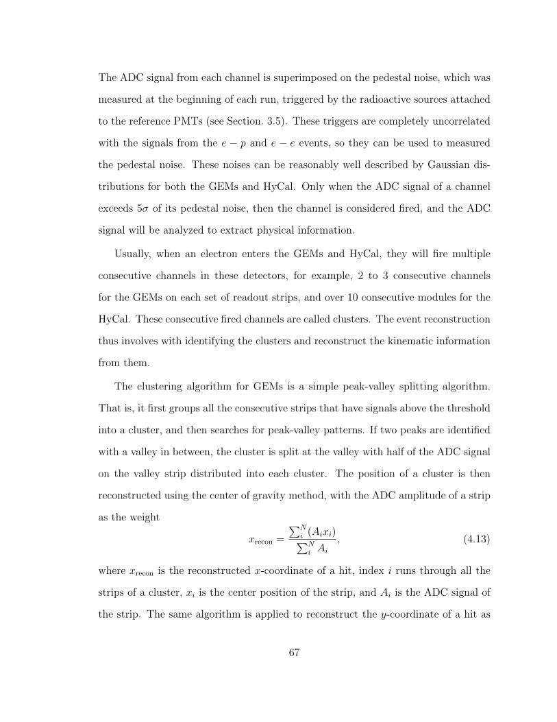
The ADC signal from each channel is superimposed on the pedestal noise, which was
measured at the beginning of each run, triggered by the radioactive sources attached
to the reference PMTs (see Section. 3.5). These triggers are completely uncorrelated
with the signals from the e − p and e − e events, so they can be used to measured
the pedestal noise. These noises can be reasonably well described by Gaussian dis-
tributions for both the GEMs and HyCal. Only when the ADC signal of a channel
exceeds 5σ of its pedestal noise, then the channel is considered fired, and the ADC
signal will be analyzed to extract physical information.
Usually, when an electron enters the GEMs and HyCal, they will fire multiple
consecutive channels in these detectors, for example, 2 to 3 consecutive channels
for the GEMs on each set of readout strips, and over 10 consecutive modules for the
HyCal. These consecutive fired channels are called clusters. The event reconstruction
thus involves with identifying the clusters and reconstruct the kinematic information
from them.
The clustering algorithm for GEMs is a simple peak-valley splitting algorithm.
That is, it first groups all the consecutive strips that have signals above the threshold
into a cluster, and then searches for peak-valley patterns. If two peaks are identified
with a valley in between, the cluster is split at the valley with half of the ADC signal
on the valley strip distributed into each cluster. The position of a cluster is then
reconstructed using the center of gravity method, with the ADC amplitude of a strip
as the weight
xrecon =
∑Ni (Aixi)∑Ni Ai
, (4.13)
where xrecon is the reconstructed x-coordinate of a hit, index i runs through all the
strips of a cluster, xi is the center position of the strip, and Ai is the ADC signal of
the strip. The same algorithm is applied to reconstruct the y-coordinate of a hit as
67

1000500
10050
10
5
1 Ener
gy d
epos
ition
[MeV
]Cluster 1
Cluster 2
Figure 4.2: Examples of HyCal cluster reconstruction for an event that has twomaxima in the same group. The two clusters are separated by finding a best matchwith the simulated cluster profiles. Reconstructed energy is obtained by taking thetotal sum of from all the modules that belong to a cluster. The reconstructed positionis evaluated using the center of gravity method in these modules.
well.
There are two cluster reconstruction algorithms implemented for the HyCal. The
first one is a 5× 5 algorithm. It firstly identifies all the modules with local maximum
energy deposition (higher ADC values than all of their neighbors), and then groups
their surrounding 5× 5 modules. This algorithm is excellent in the execution speed,
but is expected to perform less accurately in separating the scattered electron and
radiated photons. The second method is called the “island” algorithm, which is used
in the analysis. Firstly, the algorithm will group all the neighboring modules with
the signals above a certain threshold. Then it identifies the local maxima within each
group. If two or more local maxima were found in one group, the algorithm will sub-
divide the group iteratively until a best match is achieved with the simulated cluster
profiles (see Fig. 4.2). For a module that is shared by multiple clusters, its energy
distribution among the clusters is determined to achieve a maximum accordance
68

with the simulated cluster profiles. In this case, the likelihood function of a double
exponential distribution was used as the estimator. After the clustering is finished,
the reconstructed energy can be obtained from the sum of the energy depositions
from all the modules in the same cluster. The reconstructed position is obtained
from the center of gravity of the cluster with logarithmic weights, which correspond
to the exponential decay of the signal strength as a function of the distance from the
center
xrecon =
∑Ni (wixi)∑Ni wi
. (4.14)
xrecon is the reconstructed x-coordinate of a hit, index i runs through all the modules
of a cluster, xi is the center position of a module, and wi is the weighting factor of a
module
wi = Max[0, a + log(Ei/Etotal)], (4.15)
where Ei is the energy deposition in this module, Etotal is the total energy deposition
of a cluster and a is a free parameter, which when set to 3.6, gives the best position
resolution for HyCal1. This calculation is repeated to reconstruct the y-coordinate
of a hit as well.
4.3 Calibration
4.3.1 Energy Calibration
The HyCal was calibrated during the calibration runs using a photon beam, generated
by a 1.1 GeV electron beam incident on a thin wire target. The energy of the photon
beam was measured by the Hall B photon tagger [68]. There were three major
purposes for this calibration. First, the photons with tagged energies could be used
1The notation Max[a,b] means it returns the larger value between a and b.
69

Figure 4.3: The HyCal movement during the calibration runs. The photon beamwas fixed in the space, while HyCal was suspended on a transporter to move in a waysuch that the beam would hit each module one at a time in a snake-like pattern, asindicated by the red arrow.
to obtain the energy calibration constants for the HyCal modules. Second, the photon
beam energy ranged from 220 MeV to 1050 MeV (0.2 to 0.95 of the incident electron
beam energy, limited by the measurement range of the Hall B photon tagger), which
could be used to study the non-linearity properties of the HyCal modules. Third, the
events recorded in the calibration runs were triggered by the Hall B photon tagger
so that one could study the trigger efficiency of the calorimeter.
During these calibration runs, the HyCal was suspended on a transporter so that
the photon beam could be injected on each HyCal module, one at a time, in a snake-
like pattern as shown in Fig. 4.3. Once a photon enters the calorimeter, it will
generate a shower, which results in detectable signals in several consecutive modules.
A calibration constant was assigned to each module to convert the measured ADC
values into the deposited energies. A HyCal reconstruction algorithm was applied to
identify and group these modules into a cluster, and obtain the reconstructed energy
by summing the energy depositions in all the modules of the cluster. The energy
70

(Erec/E!)
Cou
nts
E! = 550 MeVSigma = 3.96%
Figure 4.4: The ratio between the reconstructed energy Erec and the beam energyEγ, for beam energy around 550 MeV. The black histogram comes from the data ofthe calibration runs, the red curve is a Gaussian fit to the data. The width (sigma) ofthe Gaussian fit is 3.96%. The figure is made by Li Ye of Mississippi State University.
calibration of the calorimeter was done iteratively, by fine tuning the calibration
constant of each module such that eventually, the reconstructed energy converged to
the energy of the incident photon. An example for the ratio between the reconstructed
energy Erec and the incident photon energy Eγ, for Eγ around 550 MeV, is shown in
Fig 4.4.
Typically, due to reasons such as the light attenuation property of a module and
the pedestal noise in the electronics, the calibration constants obtained at a particular
incident photon energy are not necessarily applicable if the incident photon is at a
different energy. The calorimeter is linear if the calibration constants can correctly
reconstruct the energy of a photon, regardless of its incident energy, otherwise, the
calorimeter is non-linear. The photon beam could be used to study this property
conveniently, as it was generated through the bremsstrahlung process and the tagged
71
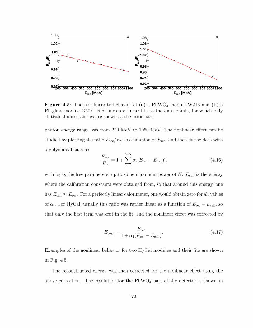
[MeV]recE200 300 400 500 600 700 800 900 1000 1100
γ/E
rec
E
0.97
0.98
0.99
1
1.01
1.02
1.03 a
[MeV]recE200 300 400 500 600 700 800 900 1000 1100
γ/E
rec
E
0.92
0.94
0.96
0.98
1
1.02
1.04
1.06
1.08 b
Figure 4.5: The non-linearity behavior of (a) a PbWO4 module W213 and (b) aPb-glass module G507. Red lines are linear fits to the data points, for which onlystatistical uncertainties are shown as the error bars.
photon energy range was from 220 MeV to 1050 MeV. The nonlinear effect can be
studied by plotting the ratio Erec/Eγ as a function of Erec, and then fit the data with
a polynomial such as
Erec
Eγ= 1 +
i=N∑i=1
αi(Erec − Ecali)i, (4.16)
with αi as the free parameters, up to some maximum power of N . Ecali is the energy
where the calibration constants were obtained from, so that around this energy, one
has Ecali ≈ Erec. For a perfectly linear calorimeter, one would obtain zero for all values
of αi. For HyCal, usually this ratio was rather linear as a function of Erec −Ecali, so
that only the first term was kept in the fit, and the nonlinear effect was corrected by
Ecorr =Erec
1 + α1(Erec − Ecali). (4.17)
Examples of the nonlinear behavior for two HyCal modules and their fits are shown
in Fig. 4.5.
The reconstructed energy was then corrected for the nonlinear effect using the
above correction. The resolution for the PbWO4 part of the detector is shown in
72

Figure 4.6: The energy resolution of the PbWO4 detector. This figure is made byMaxime Lavilain of North Carolina A&T State University.
Fig. 4.6. The resolution is about 2.5%, which is the nominal value for this detector,
based on the PrimEx measurements [63, 64, 65]. The energy resolution of Pb-glass
is much worse, at about 6%.
The third purpose of the calibration runs was to obtain the trigger efficiency
of the HyCal. During these runs, the events were recorded based on the triggers
from the photon tagger. One could then search for a trigger signal from HyCal.
The trigger efficiency was determined as the number of events that produced HyCal
triggers over the total number of events. A number of cuts were applied to suppress
the accidental backgrounds from the photon beam, including the coincidence time
between the tagger TDC and HyCal TDC signals, the HyCal energy deposition and
so on. The measured HyCal trigger efficiency is shown in Fig 4.7, for some PbWO4
and Pb-glass detectors. Typically, the efficiency reaches a plateau at about 99.9%
once the incident photon energy exceeds 400 MeV. A few low efficiency modules were
73

Figure 4.7: The trigger efficiency for PbWO4 and Pb-glass detectors, as a functionof the incident photon beam energy.
identified and removed during the analysis.
Even though for the HyCal, signals produced by electrons are highly similar to
those produced by photons, there could be some small differences [73]. In addition,
certain experimental conditions could be slightly shifted relative to those from the
calibration runs. In order to resolve these issues, the scattered electrons from the e−p
and e− e events during the production runs (the full target and empty target runs)
were also used for various purposes, such as fine tuning the calibration constants,
extracting certain fine-corrections for the HyCal reconstruction, and also fine tuning
the nonlinearity constants extracted from the photon beam calibration data. In the
first case, one would calibrate the calorimeter to the expected energies of the scattered
electrons from these reaction channels. For the e− p elastic scattering, the expected
74

exp/ErecE0.6 0.7 0.8 0.9 1 1.1 1.2 1.3 1.4
co
un
ts
0
100
200
300
400
500a
exp/ErecE0.6 0.7 0.8 0.9 1 1.1 1.2 1.3 1.4
co
un
ts
0
500
1000
1500
2000
2500
3000
3500 b
Figure 4.8: The reconstructed energy Erec over the expected energy Eexp for (a) thee− p elastic scattering and (b) the e− e elastic scattering.
energy for a scattered electron (given as equation (2.27) in Ref. [31]) is
Eexp =(Eb +M)(MEb +m2) +
√M2 −m2 sin2 θ| ~ |2 cos θ
(Eb +M)2 − | ~ |2 cos2 θ, (4.18)
where ~ is the 3-momentum of the incident electron. This formula does not neglect
the mass of an electron. If one replaces the proton mass M with the electron mass
m, one obtains the expected energy for a scattered electron from the e − e elastic
scattering,
Eexp = mEb +m+ (Eb −m) cos2 θ
Eb +m− (Eb −m) cos2 θ. (4.19)
The ratio between the reconstructed energy and the expected energy Erec/Eexp from
both e− p and e− e elastic scatterings are shown in Fig 4.8.
Secondly, certain fine-corrections for the HyCal reconstruction cannot be obtained
from the calibration runs as the incident photon beam was very narrow and it could
not cover the entire area of HyCal. These corrections are better to be obtained from
the production runs, from the e − p and e − e events. An important correction is
for the non-uniformity in the reconstructed energy from HyCal. Fig. 4.9 shows the
75

Erec/Eexp ratio for the e−p events in a PbWO4 module W5212 and a Pb-glass module
G238, as a function of the normalized reconstructed position, which is the difference
between the reconstructed position and the module center position, normalized by
the size of the module:
tx =xrec − xc
S, (4.20)
ty =yrec − yc
S, (4.21)
where the size S of a PbWO4 module is about 20.76 mm, and the size of a Pb-glass
module is about 38.15 mm. The reconstructed energy tends to be slightly larger when
the electron is hitting the edges and corners. The reason is that for the purpose of
mechanical supports, the front end of HyCal modules are covered by bronze flanges
with 2 mm thickness and a 13 mm diameter hole in the middle (see Fig. 3.11). These
flanges can behave like pre-showers, and change the shower depths of the incident
electrons. This effect is a few times larger for the Pb-glass detectors as they are more
sensitive to various shower position effects, as shown in (c) of Fig. 4.9. A detailed
description about how to correct this effect is provided in Ref. [74]. (b) and (d) of
Fig. 4.9 show the results after this correction.
Lastly, providing that the energy of the incident electron from the Møller scatter-
ing is large enough (at least 20% of the beam energy) for a particular HyCal module,
the e− p and e− e events from the production runs can also be used to fine tune the
non-linearity correction of this module, since from the calibration runs the measured
non-linearity could be well described by a linear function over the measured range.
However, the Møller electrons appearing in the Pb-glass region often have energy be-
low 200 MeV for both 1.1 and 2.2 GeV energy settings. And this linear description is
expected to break down if the energy of the incident particle is too low, which is due
2Pb-glass channel ID start with the letter ”G”, PbWO4 channels start with ”W”
76

0.5-0.4-
0.3-0.2-
0.1-0
0.10.2
0.30.4
0.5
0.5-0.4-
0.3-0.2-
0.1-0
0.10.2
0.30.4
0.50.98
0.99
1
1.01
1.02
0.98
0.99
1
1.01
1.02
avg_ep_ratio_1521
0.5-0.4-
0.3-0.2-
0.1-0
0.10.2
0.30.4
0.5
0.5-0.4-
0.3-0.2-
0.1-0
0.10.2
0.30.4
0.50.98
0.99
1
1.01
1.02
0.98
0.99
1
1.01
1.02
avg_ep_ratio_1521
𝑡" 𝑡"𝑡#𝑡#
𝐸%&'𝐸&()
𝐸%&'𝐸&()
(a) (b)
0.5-0.4-
0.3-0.2-
0.1-0
0.10.2
0.30.4
0.5
0.5-0.4-
0.3-0.2-
0.1-0
0.10.2
0.30.4
0.50.920.940.960.98
11.021.041.061.08
0.92
0.94
0.96
0.98
1
1.02
1.04
1.06
1.08
avg_ep_ratio_238
0.5-0.4-
0.3-0.2-
0.1-0
0.10.2
0.30.4
0.5
0.5-0.4-
0.3-0.2-
0.1-0
0.10.2
0.30.4
0.50.920.940.960.98
11.021.041.061.08
0.920.940.960.9811.021.041.061.08
avg_ep_ratio_238
𝑡" 𝑡"𝑡#𝑡#
𝐸%&'𝐸&()
𝐸%&'𝐸&()
(c) (d)
Figure 4.9: The non-uniformity in the HyCal reconstructed energy for e− p eventsin a PbWO4 module W521, as shown in (a), and in a Pb-glass module G238, asshown in (c). tx and ty are defined in Eq. 4.20 and Eq. 4.21. The z-axis showsthe ratio between the reconstructed energy and the expected energy, obtained usingequation Eq. 4.18. (b) and (d) show the ratio after the correction, for W521 andG238 respectively.
77
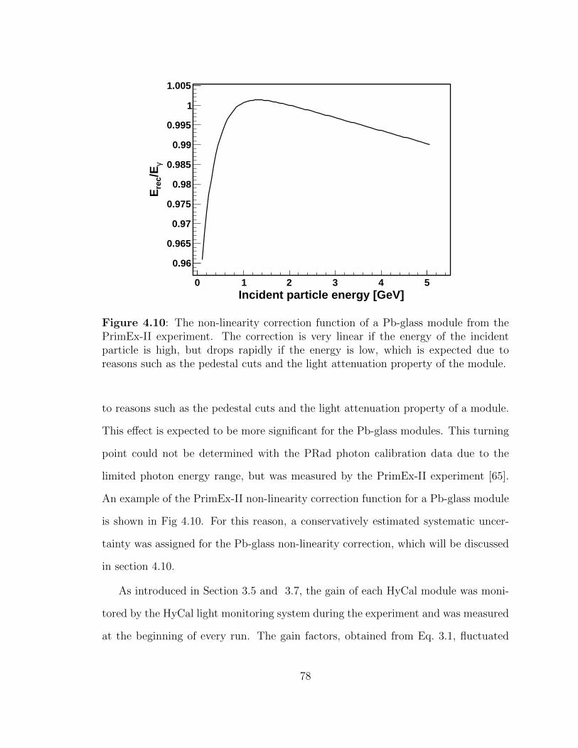
Incident particle energy [GeV]0 1 2 3 4 5
γ/E
rec
E
0.96
0.965
0.97
0.975
0.98
0.985
0.99
0.995
1
1.005
Figure 4.10: The non-linearity correction function of a Pb-glass module from thePrimEx-II experiment. The correction is very linear if the energy of the incidentparticle is high, but drops rapidly if the energy is low, which is expected due toreasons such as the pedestal cuts and the light attenuation property of the module.
to reasons such as the pedestal cuts and the light attenuation property of a module.
This effect is expected to be more significant for the Pb-glass modules. This turning
point could not be determined with the PRad photon calibration data due to the
limited photon energy range, but was measured by the PrimEx-II experiment [65].
An example of the PrimEx-II non-linearity correction function for a Pb-glass module
is shown in Fig 4.10. For this reason, a conservatively estimated systematic uncer-
tainty was assigned for the Pb-glass non-linearity correction, which will be discussed
in section 4.10.
As introduced in Section 3.5 and 3.7, the gain of each HyCal module was moni-
tored by the HyCal light monitoring system during the experiment and was measured
at the beginning of every run. The gain factors, obtained from Eq. 3.1, fluctuated
78
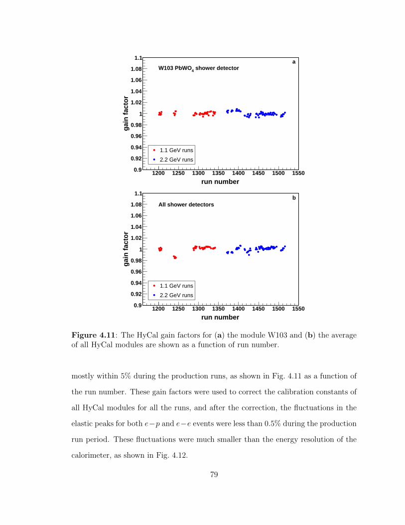
run number1200 1250 1300 1350 1400 1450 1500 1550
gai
n f
acto
r
0.9
0.92
0.94
0.96
0.98
1
1.02
1.04
1.06
1.08
1.1
shower detector4W103 PbWO a
1.1 GeV runs
2.2 GeV runs
run number1200 1250 1300 1350 1400 1450 1500 1550
gai
n f
acto
r
0.9
0.92
0.94
0.96
0.98
1
1.02
1.04
1.06
1.08
1.1
All shower detectors b
1.1 GeV runs
2.2 GeV runs
Figure 4.11: The HyCal gain factors for (a) the module W103 and (b) the averageof all HyCal modules are shown as a function of run number.
mostly within 5% during the production runs, as shown in Fig. 4.11 as a function of
the run number. These gain factors were used to correct the calibration constants of
all HyCal modules for all the runs, and after the correction, the fluctuations in the
elastic peaks for both e−p and e−e events were less than 0.5% during the production
run period. These fluctuations were much smaller than the energy resolution of the
calorimeter, as shown in Fig. 4.12.
79

Run number1200 1220 1240 1260 1280 1300 1320 1340 1360 1380
avg
/Ere
cE
0.94
0.960.98
1
1.021.04
1.06 a
Run number1200 1220 1240 1260 1280 1300 1320 1340 1360 1380
avg
/Ere
cE
0.960.970.980.99
11.011.021.031.04 b
σ1d
et. r
eso
.Run number
1360 1380 1400 1420 1440 1460 1480 1500 1520 1540
avg
/Ere
cE
0.97
0.98
0.99
1
1.01
1.02
1.03 c
Run number1360 1380 1400 1420 1440 1460 1480 1500 1520 1540
avg
/Ere
cE
0.97
0.98
0.99
1
1.01
1.02
1.03 d
σ1d
et. r
eso
.
Figure 4.12: The reconstructed elastic peak positions from each run over the aver-aged peak position from all the runs for, (a): 1.1 GeV e − p from 5.0 to 7.0, (b):1.1 GeV e−e from 1.6 to 1.8, (c): 2.2 GeV e−p from 2.5 to 3.5, and (d): 2.2 GeVe− e from 0.8 to 0.9. The fluctuation is mostly within 0.5%, and it is significantlysmaller than the detector resolution, as marked by the dash lines on each plot.
80

Detector type Energy resolution (%) Position resolution (mm)
PbWO4 2.4/√E(GeV) 2.4/
√E(GeV)
Pb-glass 6.2/√E(GeV) 6.5/
√E(GeV)
Table 4.1: The energy and position resolutions for the PbWO4 and Pb-glass showerdetectors of HyCal. E is the energy of the incident electron in unit of GeV.
The energy and position resolutions of the HyCal for the electrons from the pro-
duction runs are shown in Table 4.1. These values were used during the analysis to
determine the size of various event selection cuts.
4.3.2 Position Calibration
It is critically important to know precisely the position of the detectors as they
will directly affect the reconstructed scattering angle and Q2. The position of the
detectors and also various important components of the PRad setup (PRad target,
vacuum box window...) were surveyed by the Jefferson Lab survey group before
the experiment using their laser technique, with a precision better than 1 mm. In
addition, the e− e elastic scattering events can also be used to refine this knowledge.
For this purpose, both scattered electrons must be detected in coincidence (double-
arm Møller events). First of all, the transverse momentum conservation requires that
the transverse position of the electron beam must fall in the same plane determined by
the two scattered electrons (co-planarity). One should expect to obtain a distribution
centered at 0 if one computes the variable
∆φ = φe1 − φe2 − π, (4.22)
where φe1 and φe2 are the reconstructed azimuthal angles of the scattered electrons
from the e−e scattering, as indicated in Fig 4.13. The distributions of the co-planarity
from the data and simulation are shown in the top plot of Fig. 4.14.
81
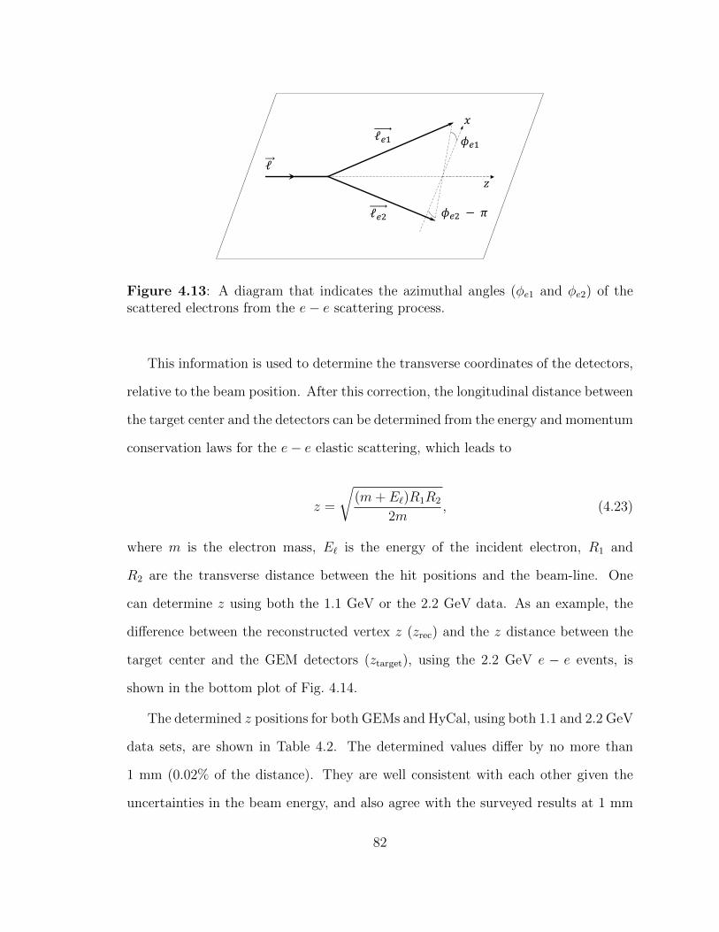
!
"
ℓ$%&
$%' − )
ℓ%&
ℓ%'
Figure 4.13: A diagram that indicates the azimuthal angles (φe1 and φe2) of thescattered electrons from the e− e scattering process.
This information is used to determine the transverse coordinates of the detectors,
relative to the beam position. After this correction, the longitudinal distance between
the target center and the detectors can be determined from the energy and momentum
conservation laws for the e− e elastic scattering, which leads to
z =
√(m+ E`)R1R2
2m, (4.23)
where m is the electron mass, E` is the energy of the incident electron, R1 and
R2 are the transverse distance between the hit positions and the beam-line. One
can determine z using both the 1.1 GeV or the 2.2 GeV data. As an example, the
difference between the reconstructed vertex z (zrec) and the z distance between the
target center and the GEM detectors (ztarget), using the 2.2 GeV e − e events, is
shown in the bottom plot of Fig. 4.14.
The determined z positions for both GEMs and HyCal, using both 1.1 and 2.2 GeV
data sets, are shown in Table 4.2. The determined values differ by no more than
1 mm (0.02% of the distance). They are well consistent with each other given the
uncertainties in the beam energy, and also agree with the surveyed results at 1 mm
82

[deg]φ∆10− 5− 0 5 10
cou
nts
/deg
0
2
4
6610×
datasimulation
[mm]target - zrecz500− 0 500
cou
nts
/mm
0
20
40
60
80
310×datasimulation
Figure 4.14: Top plot: the co-planarity distributions for the 2.2 GeV data andsimulation. Bottom plot: the difference between the reconstructed vertex z and thedistance between the target center and the GEM detectors for the 2.2 GeV data andsimulation. Only the double arm Møller events with two hits on the GEMs wereused for these computations, and the distributions were obtained based on the GEMreconstructed coordinates.
83

HyCal z (mm) GEM-I z (mm) GEM-II z (mm)1.1 GeV data 5646.56 5226.44 5186.462.2 GeV data 5645.68 5225.87 5186.43
Average 5646.12 5226.16 5186.45
Table 4.2: The longitudinal z distance between target center and detectors. GEM-Irefers to the one on beam left (looking downstream).
level. This result can be considered as a validation for the beam energy measurement
from our offline analysis, and the results were listed in Table 3.1. The averaged
positions from the two beam energy settings were used in the later analysis.
4.4 Event Selection
The event selection cuts will be discussed in this section. For all the electrons detected
by HyCal, it is required that a matching hit must be found on the GEM detectors.
First of all, all the reconstructed hits from the GEMs and HyCal are projected onto a
common transverse plane located at the surface of the PbWO4 modules, assuming the
track is produced at the center of the target cell. For each HyCal hit, the matching
GEM hits must fall inside a circle that is centered at the HyCal hit position and
with its radius determined by the position resolution of HyCal. If multiple GEM
hits satisfy this condition, then the closest one to the HyCal hit will be chosen as its
matching hit. The detectors were well aligned after the position calibration, so that
the difference of the projected coordinates from these detectors form Gaussian peaks
that are centered at 0, as shown in Fig 4.15. The size of the matching radius was
chosen to be 6 times larger than the position resolution of HyCal in order to minimize
the effects due to the non-uniformity in the HyCal coordinate reconstruction.
The second common cut applied for all the events is the dead module removal cut.
As mentioned in the previous section, a number of HyCal modules had low trigger
84
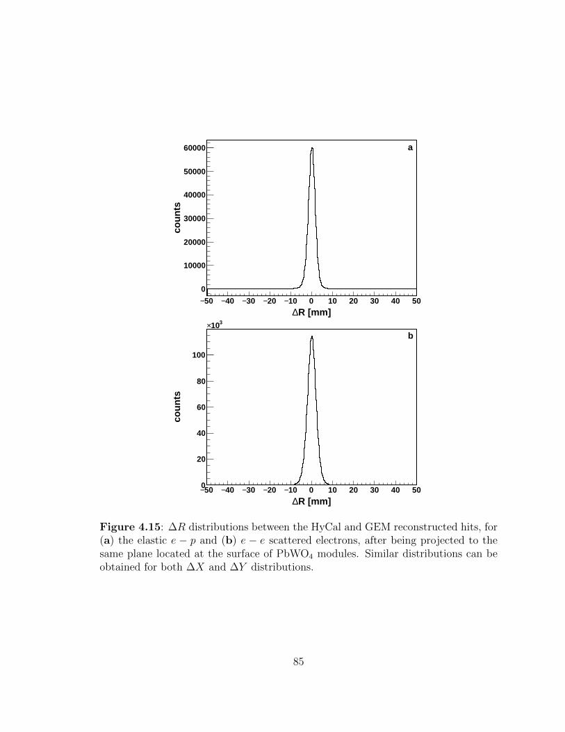
R [mm]∆50− 40− 30− 20− 10− 0 10 20 30 40 50
cou
nts
0
10000
20000
30000
40000
50000
60000 a
R [mm]∆50− 40− 30− 20− 10− 0 10 20 30 40 50
cou
nts
0
20
40
60
80
100
310×b
Figure 4.15: ∆R distributions between the HyCal and GEM reconstructed hits, for(a) the elastic e − p and (b) e − e scattered electrons, after being projected to thesame plane located at the surface of PbWO4 modules. Similar distributions can beobtained for both ∆X and ∆Y distributions.
85
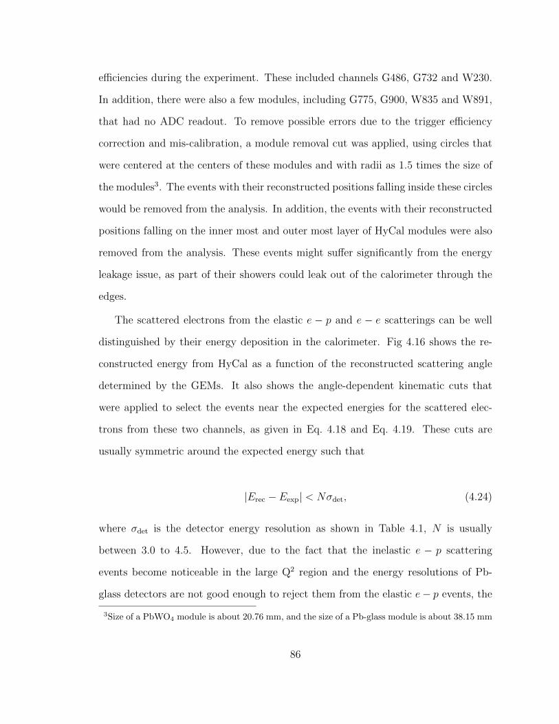
efficiencies during the experiment. These included channels G486, G732 and W230.
In addition, there were also a few modules, including G775, G900, W835 and W891,
that had no ADC readout. To remove possible errors due to the trigger efficiency
correction and mis-calibration, a module removal cut was applied, using circles that
were centered at the centers of these modules and with radii as 1.5 times the size of
the modules3. The events with their reconstructed positions falling inside these circles
would be removed from the analysis. In addition, the events with their reconstructed
positions falling on the inner most and outer most layer of HyCal modules were also
removed from the analysis. These events might suffer significantly from the energy
leakage issue, as part of their showers could leak out of the calorimeter through the
edges.
The scattered electrons from the elastic e − p and e − e scatterings can be well
distinguished by their energy deposition in the calorimeter. Fig 4.16 shows the re-
constructed energy from HyCal as a function of the reconstructed scattering angle
determined by the GEMs. It also shows the angle-dependent kinematic cuts that
were applied to select the events near the expected energies for the scattered elec-
trons from these two channels, as given in Eq. 4.18 and Eq. 4.19. These cuts are
usually symmetric around the expected energy such that
|Erec − Eexp| < Nσdet, (4.24)
where σdet is the detector energy resolution as shown in Table 4.1, N is usually
between 3.0 to 4.5. However, due to the fact that the inelastic e − p scattering
events become noticeable in the large Q2 region and the energy resolutions of Pb-
glass detectors are not good enough to reject them from the elastic e− p events, the
3Size of a PbWO4 module is about 20.76 mm, and the size of a Pb-glass module is about 38.15 mm
86
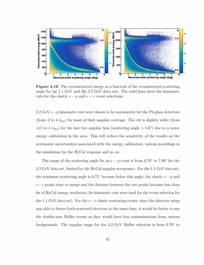
Figure 4.16: The reconstructed energy as a function of the reconstructed scatteringangle for (a) 1.1 GeV and (b) 2.2 GeV data sets. The solid lines show the kinematiccuts for the elastic e− p and e− e event selections.
2.2 GeV e−p kinematic cuts were chosen to be asymmetric for the Pb-glass detectors
(from -2 to 4 σdet) for most of their angular coverage. The cut is slightly wider (from
-2.5 to 4 σdet) for the last two angular bins (scattering angle > 5.6) due to a worse
energy calibration in the area. This will reduce the sensitivity of the results on the
systematic uncertainties associated with the energy calibration, various modelings in
the simulation for the HyCal response and so on.
The range of the scattering angle for an e− p event is from 0.70 to 7.00 for the
2.2 GeV data set, limited by the HyCal angular acceptance. For the 1.1 GeV data set,
the minimum scattering angle is 0.75 because below this angle, the elastic e− p and
e− e peaks start to merge and the distance between the two peaks becomes less than
6σ of HyCal energy resolution (3σ kinematic cuts were used for the event selection for
the 1.1 GeV data set). For the e−e elastic scattering events, since the detector setup
was able to detect both scattered electrons at the same time, it would be better to use
the double-arm Møller events as they would have less contaminations from various
backgrounds. The angular range for the 2.2 GeV Møller selection is from 0.70 to
87

2.00 and from 0.75 to 4.00 for the 1.1 GeV Møller4. The minimum scattering
angles are limited by the same reason as for the e − p events, while the maximum
scattering angles for Møller are limited by the minimum ones as they are completely
correlated.
In addition, for the double-arm Møller event selection, one could apply additional
cuts, such as the co-planarity cut, which requires the azimuthal angle difference
between the two scattered electrons to be about 180
|φe1 − φe2 − π| < 10, (4.25)
the elasticity cut, which means the total energy of the two scattered electrons must
agree with the initial beam energy
|Etotal − Eb −m| = |Ee1 + Ee2 − Eb −m| < Nσdet. (4.26)
And lastly, one can apply a cut on the reconstructed vertex-z, calculated from
Eq. 4.23, in order to ensure that the Møller event is coming from the target region.
In principle, if one requires both e−e scattered electrons to be detected at the same
time by the GEM detectors, the GEM efficiency needs to be εe−e = εe−e(θ1)×εe−e(θ2),
where θ1 and θ2 are the scattering angles of the two e− e electrons. In this way, the
GEM efficiency for e − e would be inevitably different from the GEM efficiency for
e − p, which only depends on the scattering angle of one electron. And there will
be no cancellation for the GEM efficiency regardless how one forms the e − p to
e− e ratio. This difficulty can be overcome by using a combinatory Møller selection
method. First of all, one uses only HyCal and apply the above mentioned Møller
selection cuts to select the double arm Møller events. And then after matching
4Most of the double-arm Møllers are inside the PbWO4 detector region.
88

Beam energy Category Cut
1.1 GeVKinematic cut in PbWO4
Kinematic cut in Pb-glassAngular cut
−3.0 · σdet < Erec − Eexp < 3.0 · σdet
−3.0 · σdet < Erec − Eexp < 3.0 · σdet
0.75 < θrec < 7.00
2.2 GeV
Kinematic cut in PbWO4
Kinematic cut I in Pb-glassKinematic cut II in Pb-glass
Angular cut
−3.5 · σdet < Erec − Eexp < 3.5 · σdet
−2.0 · σdet < Erec − Eexp < 4.0 · σdet
−2.5 · σdet < Erec − Eexp < 4.0 · σdet
0.70 < θrec < 7.00
Table 4.3: Selection cuts for e−p elastic scattering events. Erec is the reconstructedenergy by HyCal, Eexp is the expected energy at a given angle based on elastic e− pkinematics, σdet is the energy resolution of a HyCal module (see Table 4.1) and θrec
is the reconstructed scattering angle. In the case of 2.2 GeV beam setting, kinematiccut II in Pb-glass is used if the scattering angle is larger than 5.6 in order to reducethe sensitivity of the result on the size of this cut. Otherwise, kinematic cut I is used.
with the GEM detectors, one only uses the electron that has a matching hit on
GEMs (two if both are matched), and do not requires that both e− e electrons have
matching hits at the same time. In this way, the GEM efficiency correction factor
for the Møller counts in an angular bin θ is still εe−e(θ), which is similar to that for
the e − p events. This method is still superior in suppressing various backgrounds
from the beam-line, and the energy-independent part of the GEM efficiency can still
be cancelled if one takes the ratio between e − p and e − e counts from the same
angular bin. However, the efficiency and acceptance effects from HyCal will not be
cancelled, and one has to make a corresponding correction based on the simulation.
In addition, when applying the co-planarity and vertex-z cuts, one has to use the
HyCal reconstructed coordinates. These co-planarity and vertex-z distributions from
the data and the simulation are shown in Fig. 4.17. The event selection cuts are
summarized in Table 4.3 and Tabel 4.4, for the e− p and e− e events, respectively.
The GEM matching cuts and the dead module removal cuts are not listed in the
tables as they are universal regardless of the reaction channels.
89

[deg]φ∆20− 10− 0 10 20
cou
nts
/deg
0
0.5
1
1.5
2
610×datasimulation
[mm]target - zrecz1000− 500− 0 500 1000
cou
nts
/mm
0
10
20
30
40310×
datasimulation
Figure 4.17: Top plot: the co-planarity distributions for the 2.2 GeV data andsimulation. Bottom plot: the difference between the reconstructed vertex z and thedistance between the target center and the HyCal for the 2.2 GeV data and simula-tion. The distributions were obtained using the HyCal reconstructed coordinates.
90
Beam energy Category Cut
1.1 GeV
Kinematic cut in PbWO4
Kinematic cut in Pb-glassAngular cut
Elasticity cutCo-planarity cut
vertex-z cut
−3.0 · σdet < Erec − Eexp < 3.0 · σdet
−3.0 · σdet < Erec − Eexp < 3.0 · σdet
0.75 < θrec < 4.00
|Etotal − Eb| < 3.0 · σdet
|φe1 − φe2 − π| < 10
|zrec − ztarget| < 500 mm
2.2 GeV
Kinematic cut in PbWO4
Kinematic cut in Pb-glassAngular cut
Elasticity cutCo-planarity cut
vertex-z cut
−4.5 · σdet < Erec − Eexp < 4.5 · σdet
−4.5 · σdet < Erec − Eexp < 4.5 · σdet
0.70 < θrec < 2.00
|Etotal − Eb| < 4.5 · σdet
|φe1 − φe2 − π| < 10
|zrec − ztarget| < 500 mm
Table 4.4: Selection cuts for e−e elastic scattering events. Erec is the reconstructedenergy by HyCal, Eexp is the expected energy at an given angle based on elastice − p kinematics, σdet is the energy resolution of a HyCal module (see Table 4.1),θrec is the reconstructed scattering angle, φe1 and φe2 are the reconstructed azimuthalangles of the two scattered electrons, zrec is the reconstructed vertex-z and ztarget isthe distance between the target center and the detectors.
4.5 Background Subtraction
Not all the events that satisfy the event selection cuts are coming from the reactions
of interest. Some of them may come from the interaction of the electron beam
halo with other objects near the beam-line, such as the upstream beam halo blocker
and the target cell windows, the electron beam interaction with the background H2
gas outside the target cell, etc. While such backgrounds can be subtracted using the
empty target runs, some other backgrounds cannot be treated this way. These include
the backgrounds from the inelastic e− p scattering channels, multiple scatterings of
the small angle e−p and e−e events from downstream objects around the beam-line,
and also the photon induced hits on the GEMs through processes like pair production
and small angle Compton scattering. In the following sub-sections, the details about
subtracting these backgrounds will be discussed.
91
4.5.1 Background from Beam-Line
To subtract the backgrounds in this category, an empty target run was taken every few
hours during the production data taking of the experiment. These empty target runs
((b) in Fig 4.18) had all experimental conditions the same as for the full target runs
((a) in Fig. 4.18), except that the H2 gas was filled through a second inlet, directly
into the target chamber instead of the cell, in order to mimic the background gas
distribution far away from the target when the data taking was for the full target.
They also included contributions from the backgrounds that were generated from
objects near the beam-line, such as the upstream beam halo blocker and the target
cell window foils. The e−p and e−e counts from these runs were first normalized by
the total live charge (Eq. 3.5), and then subtracted from the corresponding counts
from the full target runs, before forming the e−p to e−e ratio. (c) and (d) in Fig. 4.18
were used to study the background contribution from some individual sources. For
instance, after normalization by the live charges, one can subtract (c) from (b) in
order to obtain backgrounds generated from the background H2 gas, and one can
study the backgrounds generated from the target cell windows by subtracting (d)
from (c). The backgrounds from (d) were mainly generated by the beam halo hitting
the upstream beam halo blocker.
The ratios between the e− p and e− e counts from the background runs ((b), (c)
and (d) in Fig. 4.18) and those from the full target runs are shown in Fig. 4.19, for
the 2.2 GeV e−p and e−e events. For the 2.2 GeV e−p events, the background rate
is high at nearly 10% of the full target rate in the forward angular region (< 1.1) due
to the backgrounds generated from the upstream beam halo blocker, otherwise the
background ratio is around or below 2%. For e−e, the ratio is much lower in general,
due to the coincidence measurement of the two scattered electrons. For both cases,
92

(a)
(b)
(c)
(d)
Figure 4.18: Main target configurations during the PRad data taking. In (a) fulltarget runs, H2 gas was filled directly into the target cell, as marked by the pink area.Blue area stands for low pressure background H2 gas from the orifices of the cell. (b)is for the empty target runs, H2 gas was filled directly into the chamber though asecond inlet to mimic background H2 gas far away from the cell. These runs wereused for the beam line background subtraction of the full target runs. No H2 gasfilled to the target system at all for (c) and (d), as marked by the white area. Theywere used to study background contributions from individual sources.
93
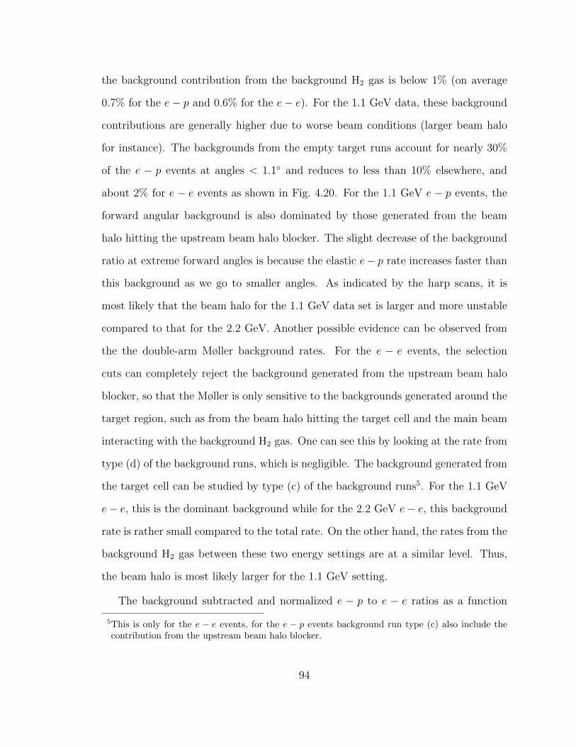
the background contribution from the background H2 gas is below 1% (on average
0.7% for the e− p and 0.6% for the e− e). For the 1.1 GeV data, these background
contributions are generally higher due to worse beam conditions (larger beam halo
for instance). The backgrounds from the empty target runs account for nearly 30%
of the e − p events at angles < 1.1 and reduces to less than 10% elsewhere, and
about 2% for e − e events as shown in Fig. 4.20. For the 1.1 GeV e − p events, the
forward angular background is also dominated by those generated from the beam
halo hitting the upstream beam halo blocker. The slight decrease of the background
ratio at extreme forward angles is because the elastic e− p rate increases faster than
this background as we go to smaller angles. As indicated by the harp scans, it is
most likely that the beam halo for the 1.1 GeV data set is larger and more unstable
compared to that for the 2.2 GeV. Another possible evidence can be observed from
the the double-arm Møller background rates. For the e − e events, the selection
cuts can completely reject the background generated from the upstream beam halo
blocker, so that the Møller is only sensitive to the backgrounds generated around the
target region, such as from the beam halo hitting the target cell and the main beam
interacting with the background H2 gas. One can see this by looking at the rate from
type (d) of the background runs, which is negligible. The background generated from
the target cell can be studied by type (c) of the background runs5. For the 1.1 GeV
e− e, this is the dominant background while for the 2.2 GeV e− e, this background
rate is rather small compared to the total rate. On the other hand, the rates from the
background H2 gas between these two energy settings are at a similar level. Thus,
the beam halo is most likely larger for the 1.1 GeV setting.
The background subtracted and normalized e − p to e − e ratios as a function
5This is only for the e − e events, for the e − p events background run type (c) also include thecontribution from the upstream beam halo blocker.
94

Reconstructed scattering angle [deg]1−10×6 1 2 3 4 5 6 7 8 9 10
tota
l/N
bac
kgro
un
dN
0
0.02
0.04
0.06
0.08
0.1
(b)(c)(d)(b) - (c)
a
Reconstructed scattering angle (deg)0.6 0.8 1 1.2 1.4 1.6 1.8 2
tota
l/N
bac
kgro
un
dN
0
0.001
0.002
0.003
0.004
0.005
0.006
0.007
0.008
0.009
0.01 b
Figure 4.19: The counts from the runs with target configuration (b), (c) (d) inFig. 4.18 over that from the full target runs. Plot (a) shows the ratios for 2.2 GeVe− p events, Plot (b) is for 2.2 GeV e− e events.
95
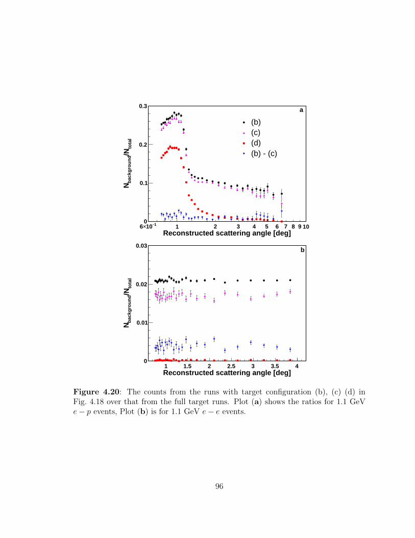
Reconstructed scattering angle [deg]1−10×6 1 2 3 4 5 6 7 8 9 10
tota
l/N
bac
kgro
un
dN
0
0.1
0.2
0.3
(b)(c)(d)(b) - (c)
a
Reconstructed scattering angle [deg]1 1.5 2 2.5 3 3.5 4
tota
l/N
bac
kgro
un
dN
0
0.01
0.02
0.03b
Figure 4.20: The counts from the runs with target configuration (b), (c) (d) inFig. 4.18 over that from the full target runs. Plot (a) shows the ratios for 1.1 GeVe− p events, Plot (b) is for 1.1 GeV e− e events.
96
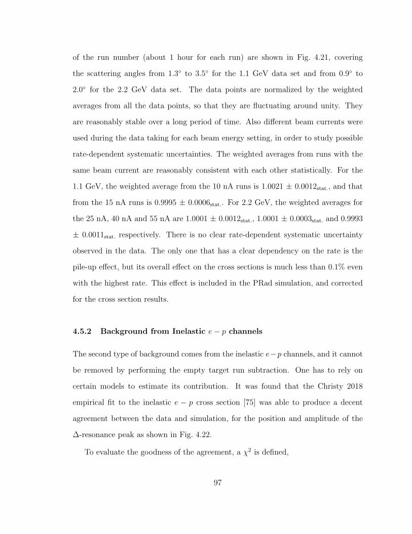
of the run number (about 1 hour for each run) are shown in Fig. 4.21, covering
the scattering angles from 1.3 to 3.5 for the 1.1 GeV data set and from 0.9 to
2.0 for the 2.2 GeV data set. The data points are normalized by the weighted
averages from all the data points, so that they are fluctuating around unity. They
are reasonably stable over a long period of time. Also different beam currents were
used during the data taking for each beam energy setting, in order to study possible
rate-dependent systematic uncertainties. The weighted averages from runs with the
same beam current are reasonably consistent with each other statistically. For the
1.1 GeV, the weighted average from the 10 nA runs is 1.0021 ± 0.0012stat., and that
from the 15 nA runs is 0.9995 ± 0.0006stat.. For 2.2 GeV, the weighted averages for
the 25 nA, 40 nA and 55 nA are 1.0001 ± 0.0012stat., 1.0001 ± 0.0003stat. and 0.9993
± 0.0011stat. respectively. There is no clear rate-dependent systematic uncertainty
observed in the data. The only one that has a clear dependency on the rate is the
pile-up effect, but its overall effect on the cross sections is much less than 0.1% even
with the highest rate. This effect is included in the PRad simulation, and corrected
for the cross section results.
4.5.2 Background from Inelastic e− p channels
The second type of background comes from the inelastic e−p channels, and it cannot
be removed by performing the empty target run subtraction. One has to rely on
certain models to estimate its contribution. It was found that the Christy 2018
empirical fit to the inelastic e − p cross section [75] was able to produce a decent
agreement between the data and simulation, for the position and amplitude of the
∆-resonance peak as shown in Fig. 4.22.
To evaluate the goodness of the agreement, a χ2 is defined,
97
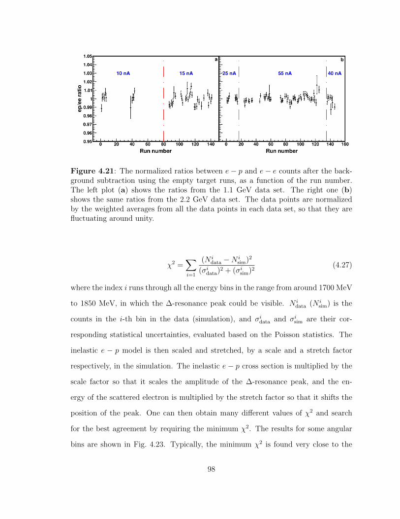
Figure 4.21: The normalized ratios between e− p and e− e counts after the back-ground subtraction using the empty target runs, as a function of the run number.The left plot (a) shows the ratios from the 1.1 GeV data set. The right one (b)shows the same ratios from the 2.2 GeV data set. The data points are normalizedby the weighted averages from all the data points in each data set, so that they arefluctuating around unity.
χ2 =∑i=1
(N idata −N i
sim)2
(σidata)2 + (σisim)2(4.27)
where the index i runs through all the energy bins in the range from around 1700 MeV
to 1850 MeV, in which the ∆-resonance peak could be visible. N idata (N i
sim) is the
counts in the i-th bin in the data (simulation), and σidata and σisim are their cor-
responding statistical uncertainties, evaluated based on the Poisson statistics. The
inelastic e − p model is then scaled and stretched, by a scale and a stretch factor
respectively, in the simulation. The inelastic e− p cross section is multiplied by the
scale factor so that it scales the amplitude of the ∆-resonance peak, and the en-
ergy of the scattered electron is multiplied by the stretch factor so that it shifts the
position of the peak. One can then obtain many different values of χ2 and search
for the best agreement by requiring the minimum χ2. The results for some angular
bins are shown in Fig. 4.23. Typically, the minimum χ2 is found very close to the
98

Kinematic cut
Kinematic cut
Figure 4.22: The comparison between the reconstructed energy spectrum from the2.2 GeV data (black) and the simulation (red) for part of the PbWO4 detector region(a) and Pb-glass detector region (b). (a) covers scattering angle from 3.0 to 3.3,which corresponds to Q2 around 0.014 (GeV/c)2. (b) covers scattering angle from6.0 to 7.0, which corresponds to Q2 around 0.059 (GeV/c)2 (largest Q2 for PRad).Blue histograms show the inelastic e− p contribution from the simulation, using theChristy 2018 model. Due to a large difference in amplitudes, the elastic e − p peak(amplitude 2800 counts/MeV) is not shown in (a), in order to display the ∆-resonancepeak.
99

original Christy 2018 model (scale factor = 1 and stretch factor = 1), particularly for
the PbWO4 region where there is a clear separation between the ∆-resonance peak
and the elastic e − p peak (see (a) in Fig. 4.22). The scale factor is found typically
from 0.9 to 1.1 for the minimum χ2, and from 0.995 to 1.005 for the stretch factor.
For Pb-glass region, the agreement can be slightly worse for certain angular bins, for
example, the minimum χ2 for scattering angles from 6.0 to 7.0 (shown in (b) of
Fig. 4.22) appears when the stretch factor is 1.01 and the scale factor is 0.9. This is
most likely due to the nonlinear properties of the Pb-glass modules, which may also
shift the position of the ∆-resonance peak. One may disentangle these two effects
by studying the spectrum agreement in the polar-angle overlapping region between
the PbWO4 detectors and the Pb-glass detectors, and the agreement was found to
be better in the PbWO4 detectors. However, this study cannot be applied reliably
to the 1.1 GeV data set as the inelastic e − p contribution is much smaller and the
∆-resonance peak is not clearly visible anywhere. It is assumed that for the 1.1 GeV
data set, the scale factor and the stretch factor would also be in the range from 0.9
to 1.1, and 0.995 to 1.005, respectively.
With the Christy 2018 model, the inelastic e− p contribution is estimated to be
negligible in the PbWO4 region. Due to the good energy resolution, the kinematic cut
for e−p event selection is sufficiently good to reject most of the inelastic e−p events,
as shown in Fig. 4.22. However, for Pb-glass detectors, the tail from the ∆-resonance
peak starts to leak under the e − p elastic peak, due to a worse detector resolution.
The contribution is determined as no more than 2% and 0.2%, for the 2.2 GeV and
1.1 GeV data sets, respectively, and the contribution increases with larger Q2.
100

scale factor0.7 0.8 0.9 1 1.1 1.2 1.3
stre
tch
fac
tor
0.97
0.98
0.99
1
1.01
1.02
1.03
1.04
1.05
2 χ
0
100
200
300
400
500
600
700a
scale factor0.7 0.8 0.9 1 1.1 1.2 1.3
stre
tch
fac
tor
0.97
0.98
0.99
1
1.01
1.02
1.03
1.04
1.05
2 χ
0
100
200
300
400
500b
Figure 4.23: χ2 from Eq. 4.27, as a function of scale factor and stretch factorfor the 2.2 GeV beam energy setting. (a) is for the scattering angles from 3.0 to3.3, corresponding to Q2 of 0.014 (GeV/c)2, (b) is for the scattering angles from4.0 to 4.3, corresponding to Q2 of 0.024 (GeV/c)2. The red boxes mark the cellcorresponding to the minimum χ2. The minimum χ2/ndf is about 0.67 for (a) and1.11 for (b).
101
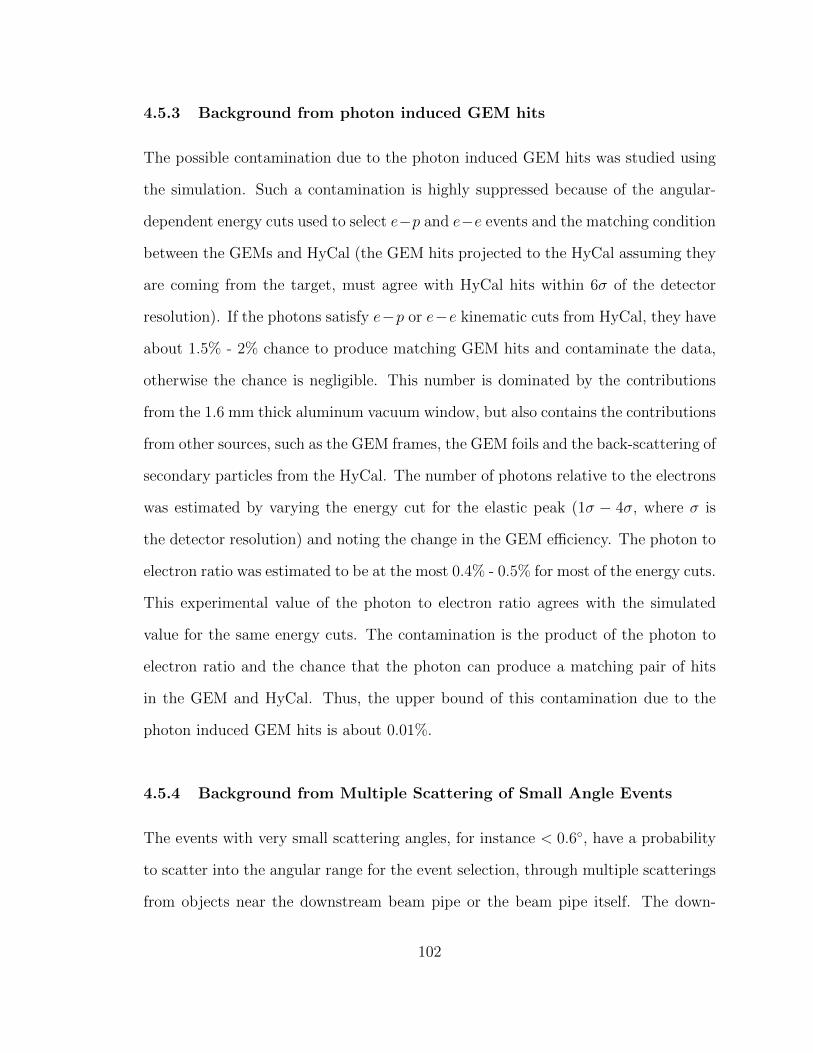
4.5.3 Background from photon induced GEM hits
The possible contamination due to the photon induced GEM hits was studied using
the simulation. Such a contamination is highly suppressed because of the angular-
dependent energy cuts used to select e−p and e−e events and the matching condition
between the GEMs and HyCal (the GEM hits projected to the HyCal assuming they
are coming from the target, must agree with HyCal hits within 6σ of the detector
resolution). If the photons satisfy e−p or e−e kinematic cuts from HyCal, they have
about 1.5% - 2% chance to produce matching GEM hits and contaminate the data,
otherwise the chance is negligible. This number is dominated by the contributions
from the 1.6 mm thick aluminum vacuum window, but also contains the contributions
from other sources, such as the GEM frames, the GEM foils and the back-scattering of
secondary particles from the HyCal. The number of photons relative to the electrons
was estimated by varying the energy cut for the elastic peak (1σ − 4σ, where σ is
the detector resolution) and noting the change in the GEM efficiency. The photon to
electron ratio was estimated to be at the most 0.4% - 0.5% for most of the energy cuts.
This experimental value of the photon to electron ratio agrees with the simulated
value for the same energy cuts. The contamination is the product of the photon to
electron ratio and the chance that the photon can produce a matching pair of hits
in the GEM and HyCal. Thus, the upper bound of this contamination due to the
photon induced GEM hits is about 0.01%.
4.5.4 Background from Multiple Scattering of Small Angle Events
The events with very small scattering angles, for instance < 0.6, have a probability
to scatter into the angular range for the event selection, through multiple scatterings
from objects near the downstream beam pipe or the beam pipe itself. The down-
102
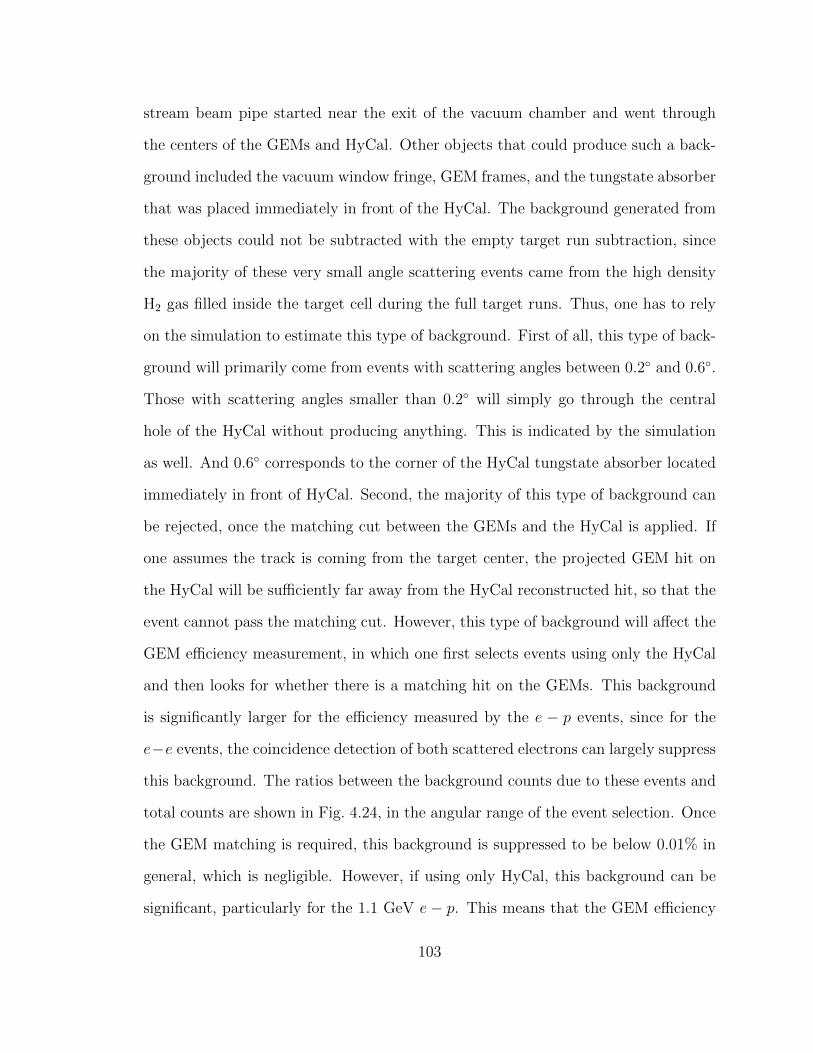
stream beam pipe started near the exit of the vacuum chamber and went through
the centers of the GEMs and HyCal. Other objects that could produce such a back-
ground included the vacuum window fringe, GEM frames, and the tungstate absorber
that was placed immediately in front of the HyCal. The background generated from
these objects could not be subtracted with the empty target run subtraction, since
the majority of these very small angle scattering events came from the high density
H2 gas filled inside the target cell during the full target runs. Thus, one has to rely
on the simulation to estimate this type of background. First of all, this type of back-
ground will primarily come from events with scattering angles between 0.2 and 0.6.
Those with scattering angles smaller than 0.2 will simply go through the central
hole of the HyCal without producing anything. This is indicated by the simulation
as well. And 0.6 corresponds to the corner of the HyCal tungstate absorber located
immediately in front of HyCal. Second, the majority of this type of background can
be rejected, once the matching cut between the GEMs and the HyCal is applied. If
one assumes the track is coming from the target center, the projected GEM hit on
the HyCal will be sufficiently far away from the HyCal reconstructed hit, so that the
event cannot pass the matching cut. However, this type of background will affect the
GEM efficiency measurement, in which one first selects events using only the HyCal
and then looks for whether there is a matching hit on the GEMs. This background
is significantly larger for the efficiency measured by the e − p events, since for the
e−e events, the coincidence detection of both scattered electrons can largely suppress
this background. The ratios between the background counts due to these events and
total counts are shown in Fig. 4.24, in the angular range of the event selection. Once
the GEM matching is required, this background is suppressed to be below 0.01% in
general, which is negligible. However, if using only HyCal, this background can be
significant, particularly for the 1.1 GeV e − p. This means that the GEM efficiency
103

Reconstructed scattering angle [deg]1 2 3 4 5 6 7
Rat
io [
%]
0
0.1
0.2
0.3
0.4
0.5
0.6
0.7Only HyCal
HyCal and GEMs
a
Reconstructed scattering angle [deg]0.5 1 1.5 2 2.5 3 3.5 4
Rat
io [
%]
0
0.005
0.01
0.015
0.02
0.025
0.03 b
Reconstructed scattering angle [deg]1 2 3 4 5 6 7
Rat
io [
%]
0
0.01
0.02
0.03
0.04
0.05
0.06
0.07 c
Reconstructed scattering angle [deg]0.8 1 1.2 1.4 1.6 1.8
Rat
io [
%]
0
0.005
0.01
0.015
0.02d
Figure 4.24: The ratio between background counts due to the events with scatteringangles from 0.2 to 0.6 and the total counts using the PRad simulation, for (a):1.1 GeV e− p, (b): 1.1 GeV e− e, (c): 2.2 GeV e− p and (d): 2.2 GeV e− e. Blackdots are obtained using only the HyCal. Red squares are obtained after requiringthere is a matching hit on the GEMs.
measured using the e−p events can be underestimated in the forward angular region.
The inefficiency due to this background is corrected using the simulation and since
it affects mostly scattering angles less than 1.3, for which the bin-by-bin method
is applied and the GEM efficiency is not needed, the systematic uncertainty for this
correction is considered negligible for the results.
104

4.6 Efficiency of GEM
The GEM efficiency was determined using both the e− p and e− e events from the
production runs. During this process, the events of interest were first identified using
the HyCal reconstructed information alone and then one would search if there were
matching GEM hits. If there were, then the GEMs were counted as efficient. All the
event selection cuts for e− p and e− e were applied to this study, with much tighter
cuts (1σ of the HyCal energy resolution) on the energy of the scattered electrons in
order to reject high energy radiated photons, cosmic events and other backgrounds.
A cluster profile cut was also applied, which put requirements on the size and shape
of a cluster, in order to further reject the cosmic events. A background subtraction
using the empty target runs was also performed for the efficiency calculation. In this
case, the efficiency could be calculated as
εGEM =N full
GEM − C·NempGEM
N fullHyCal − C·N
empHyCal
, (4.28)
where N is the number of counts, the subscripts “GEM” and “HyCal” indicate which
detector they come from, and the superscripts “full” and “emp” indicate that the
counts are from the full target runs and the empty target runs, respectively. C is the
live charge ratio between the full target and empty target runs. The statistical un-
certainties were estimated using the Binomial statistics. Notice that the backgrounds
generated from the electron beam should be scaled with the live charge while the cos-
mic backgrounds should be scaled with the total time (weighted by DAQ live time)
of the data taking. Thus, the runs and periods with an unstable beam status were
removed from this study so that C is also about the same as the total time ratio
between the full target runs and the empty target runs, as shown in Fig. 4.25. The
data point for the first sub-period of the 1.1 GeV data set ((a) of Fig. 4.25) had a
105

beam stability issue, which is the reason that its data point is far away from unity,
and thus it was excluded in the entire analysis. Otherwise, the live charge ratios agree
with the total time ratios mostly within 0.2%. This enables a subtraction of the cos-
mic backgrounds as well. The background subtracted GEM efficiencies for e− p and
e− e events for various scattering angles are shown in Fig. 4.26. The efficiencies are
very stable regardless of the size of the energy cut. In the case of the 1.1 GeV beam
energy setting, the kinematic cut variation is limited to 3σ as the e − p and e − e
events can not be well distinguished at very forward angles if a larger cut is used.
Typically, the variation on the efficiency is smaller than 0.2% except for the efficiency
in the very forward angular region measured by the 1.1 GeV e− p events. This is ex-
pected due to the background generated from the very-small-angle-scattering events
(see Section 4.5.4). Otherwise, the slight increase in the efficiency with narrower cuts
can be explained by high energy radiative photons. In addition, a machine learning
algorithm based on the auto-encoder [76] and the convolutional neural network [77]
was developed by Duke Postdoc researcher Xuefei Yan, and trained using the cosmic
runs taken during the PRad experiment in order to reject the cosmic backgrounds.
The GEM efficiency results obtained after applying this cosmic rejection algorithm
is consistent statistically with the efficiency results obtained after the background
subtraction using the empty target runs, which demonstrates that the cosmic back-
grounds were under control.
The background due to high energy radiative photons generated from the e − p
and e − e bremsstrahlung processes was studied using the generators for e − p and
e− e elastic scatterings. They included the exact calculations for the next-to-leading
order Feynman diagrams and were capable of generating radiative photons up to
nearly the energy of the incident electron beam. The effect is expected to be around
0.06% or less in the Pb-glass detector region, and <0.01% in the PbWO4 region if
106

Sub-period ID0 2 4 6 8 10 12 14
Su
per
rat
io
0.92
0.94
0.96
0.98
1a
Sub-period ID0 2 4 6 8 10 12 14 16 18
Su
per
rat
io
0.99
0.992
0.994
0.996
0.998
1
1.002
1.004
1.006
1.008
1.01b
Figure 4.25: Super ratio of the live charge ratio, between the full target and theempty target runs, over the total time (weighted by ADC live time) ratio, betweenthe full target and the empty target runs, as a function of the sub-period for thebackground subtraction. Left plot (a) for the 1.1 GeV data set, right plot (b) for the2.2 GeV data set.
using a kinematic cut with 1σ of detector resolution, and around 0.26% or less in the
Pb-glass detector region and around 0.08% in the PbWO4 region if using a kinematic
cut with 4σ of detector resolution.
The GEM efficiencies measured using the 1.1 GeV e−p and e−e events, and those
from the 2.2 GeV data set are shown in Fig. 4.27. The GEM efficiencies measured
by the e− e events have smaller angular coverage than that for the e− p events, as
the double-arm Møller event selection was applied in the study, and it would limit
the angular acceptance. These GEM efficiencies include the efficiency loss due to the
GEM spacers and the gaps between the high voltage sectors. There are a number of
reasons for the slight differences between the efficiencies measured using these two
types of events. First of all, the matching cuts between the GEMs and HyCal are
different for e − p and e − e events. The electrons from the Møller scattering have
lower energies and thus are more sensitive to the multiple scattering effect and have
worse HyCal position resolution. The matching cut for e−e events is larger than that
for the e − p events. Second, for a particular angular bin, the efficiency losses due
107

σN1 1.5 2 2.5 3
GE
M e
ffic
ien
cy
0.87
0.88
0.89
0.9
0.91
0.92
0.93
0.94
0.95
0.96
0.97 o < 0.80θ < o0.75o < 3.00θ < o2.50o < 7.00θ < o6.00
a
σN1 1.5 2 2.5 3 3.5 4
GE
M e
ffic
ien
cy0.88
0.89
0.9
0.91
0.92
0.93
0.94
0.95
0.96
0.97 o < 0.80θ < o0.70o < 3.00θ < o2.50o < 7.00θ < o6.00
b
σN1 1.5 2 2.5 3
GE
M e
ffic
ien
cy
0.9
0.91
0.92
0.93
0.94
0.95
0.96
0.97 o < 0.80θ < o0.75o < 1.80θ < o1.60o < 3.00θ < o2.50
c
σN1 1.5 2 2.5 3 3.5 4
GE
M e
ffic
ien
cy
0.93
0.935
0.94
0.945
0.95
0.955
0.96 o < 0.80θ < o0.70o < 1.40θ < o1.30o < 1.80θ < o1.60
d
Figure 4.26: GEM efficiencies for 1.1 GeV e − p (a), 2.2 GeV e − p (b), 1.1 GeVe− e (c), 2.2 GeV e− e (d) for various scattering angles as indicated in the legends,as a function of the size of the kinematic cuts, which are measured in unit of theenergy resolution of HyCal.
108

to the GEM spacers and the gaps between the high voltage sectors can be slightly
different between the e − p and e − e events, as the angular distributions for these
two types of events are very different. The e − p events always focus more on the
lower edge of an angular bin, while the e− e events tend to go to the upper edge of
a bin, particularly if the scattering angle is large. Thus, this effect is more dominant
at the large angles, such as those larger than 1.5, but this is expected and can be
reproduced using the simulation. Third, the efficiencies measured by the e−p events
are typically smaller than that from the e − e events in the forward angular region
(< 1.3), and it is more obvious in the case of the 1.1 GeV efficiencies. This is due to
the background from the very-small-angle-scattering events (see Section 4.5.4). This
background has a significantly impact on the efficiency measured by the 1.1 GeV e−p
events in the very forward angular region, and quickly becomes less than 0.1% when
the scattering angle is larger than 1.3. However, since the GEM efficiency in the
forward angular region can be cancelled by using the bin-by-bin method, the effect
due to this background is further minimized. This effect will be corrected using the
simulation and since the overall effect is expected to be less than 0.1%, the systematic
uncertainty for this correction was considered negligible. And lastly, the efficiencies
measured by the e−p and e−e events may be affected differently by the HyCal finite
resolution effect, which is in fact, one of the major systematic uncertainty sources for
the GEM efficiency measurements.
The HyCal position resolution (see Table 4.1) is not good enough to resolve the
spacers and the gaps between high voltage sectors, and also it is about the same
size as the forward angular bins. It causes a significant bin migration problem,
particularly for the very forward angular region6. One can study this effect using
6The multiple scattering can also cause a similar effect, but it is much smaller than the HyCalresolution effect.
109

[deg]θScattering angle 1 10
GE
M e
ffic
ien
cy [
%]
88
89
90
91
92
93
94
95
96ep GEM efficiency
ee GEM efficiency
[deg]θScattering angle 1 10
GE
M e
ffic
ien
cy [
%]
88
89
90
91
92
93
94
95
96 ep GEM efficiency
ee GEM efficiency
Figure 4.27: GEM efficiencies measured using (top) 1.1 GeV e−p and e− e events,and (bottom) 2.2 GeV e− p and e− e events, as a function of the scattering angle.
110

the simulation, by comparing results from the simulation that uses perfect GEM
detectors and simulation that uses more realistic GEM detectors including all the
dead areas. The GEM efficiency obtained from these two cases are shown in Fig. 4.28.
The intrinsic efficiency (probability for the ionization, avalanche, and producing a
detectable signal on the readout strips) is assumed to be 100% for this study. In the
case with no GEM spacers and dead areas, the efficiency is nearly 100%. The small
loss for the GEM efficiencies is mainly due to the finite matching radius used in the
analysis (6σ of the HyCal position resolution) and can be removed if one uses larger
ones. In the other case, the efficiency is highly non-uniform due to the GEM spacers
and the gaps between the high voltage sectors, and the inefficiency can be as large as
6%. One can study the GEM efficiency corrected e− p to e− e ratio obtained from
these two cases. If the GEM efficiency calculation and correction are accurate, one
would expect the two ratios agree with each other. However, due to the systematic
uncertainty related to the HyCal finite resolution, there can be certain deviations
from unity, and the effect is particularly large in the forward angular region. As
shown in (a) of Fig. 4.29, the deviation can be significantly larger than 0.2% at the
very forward angular region (< 1.3) for the 2.2 GeV beam energy setting, with
the maximum deviation slightly above 0.5%. This deviation is slightly larger for
the 1.1 GeV setting (about 0.7% for the maximum deviation) as the HyCal position
resolution is energy-dependent and it is better at a higher energy. To overcome this
difficulty, one can apply the bin-by-bin method when forming the e−p to e− e ratio,
that is, taking the e − p counts and e − e counts from the same angular bin. In
this case, the energy-independent part of the GEM efficiency is cancelled. This is
demonstrated in (b) of Fig. 4.29, where the forward angle data points (< 1.6) are
obtained with the bin-by-bin method. The deviation for the bin-by-bin method is no
more than 0.05% in this angular range. However, the bin-by-bin method cannot be
111
Reconstructed scattering angle [deg]0 1 2 3 4 5 6 7
GE
M e
ffic
ien
cy [
%]
92
93
94
95
96
97
98
99
100
No spacersWith spacers
Figure 4.28: The GEM efficiencies obtained from the PRad simulation. The blackdotted points are obtained with perfect GEM detectors with no spacers and no deadarea. The red squares are obtained with more realistic GEM detectors that includethe GEM spacers and the gaps between the high voltage sectors.
applied to the entire angular acceptance of HyCal if one requires the two electrons
from the e − e scattering to be detected at the same time. This is because for the
e − e scattering, if one electron goes to a large angle, the other one may hit the
HyCal tungstate absorber or even pass HyCal through its central hole, so that there
is only one electron detected. This limits the angular acceptance of the double-arm
Møllers to be less than 4.0 for the 1.1 GeV beam setting and less than 2.0 for the
2.2 GeV beam setting, and the e − p to e − e ratio in larger angular range has to
be obtained from the integrated Møller method, which requires a GEM efficiency
correction. As shown in Fig. 4.29, the deviations for the e− p to e− e ratio obtained
from the integrated Møller method at large angles are mostly within 0.2%, which is
still acceptable.
112

Reconstructed scattering angle [deg]0 1 2 3 4 5 6 7
sim
/(ep
/ee)
xsi
m(e
p/e
e)
0.99
0.995
1
1.005
1.01
a
Reconstructed scattering angle [deg]0 1 2 3 4 5 6 7
sim
/(ep
/ee)
xsi
m(e
p/e
e)
0.99
0.995
1
1.005
1.01
b
Bin by bin Integrated Moller
Figure 4.29: The GEM efficiency corrected e− p to e− e ratio from the simulationwith more realistic GEM detectors that include all the dead areas, over the same ratiofrom the simulation with perfect GEM detectors. The results in (a) are obtained usingthe integrated Møller method. For (b), the results on the left hand side of the bluedash line are obtained with the bin-by-bin method, while the results on the righthand side remain the same as those shown in (a).
The GEM efficiency measured with the 2.2 GeV e−p events, from the regions that
are far away from the spacers, is shown in Fig. 4.30. The efficiency is rather uniform
when the scattering angle is less than 3, while it drops by 5% at larger angles. This
drop was due to an issue with the front-end electronics. All the channels that were
parallel to the y−axis, in the range −460 mm < x < −200 mm, were connected to the
same Frontend Concentrator Card (FEC) during the experiment. They all suffered
from this issue, which led to early saturations for the APV channels, and resulted
in smaller ADC signals from the APV25s, compared to other channels. As a result,
the GEM efficiency in this region was more sensitive to the pedestal cuts, and the
efficiency was lower by nearly 10% compared to the efficiencies in other unaffected
regions. This efficiency drop can be reproduced very well by the simulation. To
further validate the GEM efficiency correction, the e− p to e− e ratios between the
data and the simulation from different quadrants of the detecters are compared, and
shown in Fig 4.31. Two different quadrant definitions were used in this study. In the
113
Figure 4.30: The GEM efficiency measured using 2.2 GeV e−p events, from regionsthat have no GEM spacers. This figure is made by Xinzhan Bai of University ofVirginia.
first case, the y-axis is vertical to the ground and the x-axis is to the right if one looks
downstream towards the detectors. In the second case, the x − y plane is rotate by
45 clockwise around the z-axis. The ratios, after the GEM efficiency correction, are
consistent within their statistical uncertainties for all the angular bins. Lastly, one
can study the extracted e− p elastic scattering cross sections in the Q2 overlapping
region between the 1.1 GeV and 2.2 GeV data sets (more details in Section 4.9.3).
This efficiency drop is the same for both 1.1 GeV and 2.2 GeV data sets. If this
drop is artificial, it will cause the 1.1 GeV data point at the highest Q2 (about 0.016
(GeV/c)2) to shift by nearly 5%, while its statistical uncertainty is about 1%. On
the other hand, for the 2.2 GeV data set, the data point at the same Q2 will not be
affected by the drop as the corresponding scattering angle is about 3.4. This will
cause a significantly discrepancy between the two data sets, which is not observed
as their cross section data points are highly consistent statistically around this Q2
value. To sum up, we are confident that this decrease of the GEM efficiency at large
114
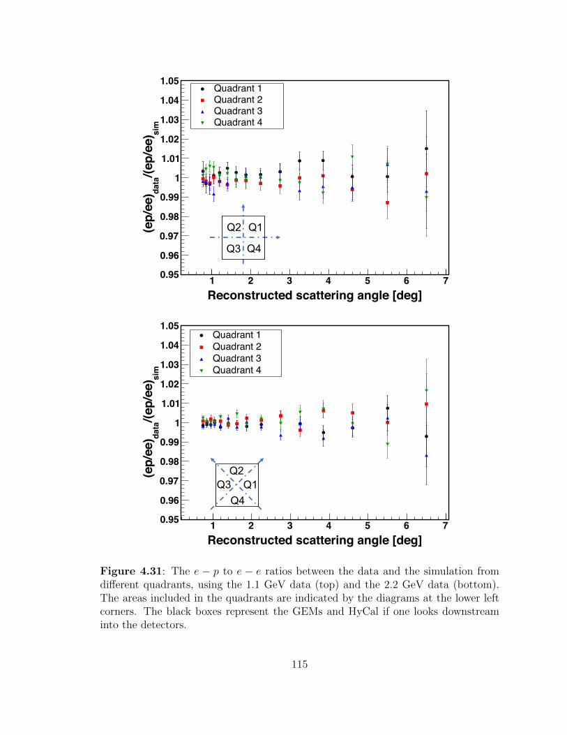
Reconstructed scattering angle [deg]1 2 3 4 5 6 7
sim
/(ep/
ee)
data
(ep/
ee)
0.95
0.96
0.97
0.98
0.99
1
1.01
1.02
1.03
1.04
1.05Quadrant 1Quadrant 2Quadrant 3Quadrant 4
Q1Q2
Q3 Q4
Reconstructed scattering angle [deg]1 2 3 4 5 6 7
sim
/(ep/
ee)
data
(ep/
ee)
0.95
0.96
0.97
0.98
0.99
1
1.01
1.02
1.03
1.04
1.05Quadrant 1Quadrant 2Quadrant 3Quadrant 4
Q1Q2
Q3Q4
Figure 4.31: The e − p to e − e ratios between the data and the simulation fromdifferent quadrants, using the 1.1 GeV data (top) and the 2.2 GeV data (bottom).The areas included in the quadrants are indicated by the diagrams at the lower leftcorners. The black boxes represent the GEMs and HyCal if one looks downstreaminto the detectors.
115

angles was indeed due to the electronic issue and it can be corrected successfully by
the GEM efficiency correction.
4.7 Simulation
As mentioned at the beginning of this chapter, the analysis of this experiment re-
quires a comprehensive and realistic Monte Carlo simulation. This is necessary for
the studies of the acceptance, radiative effects, bin center correction, various sys-
tematic uncertainties and so on. A simulation program was developed based on the
Geant4 toolkit [78], which is capable of calculating possible radiative effects such as
the energy loss and bremsstrahlung radiation, and multiple scatterings as particles
pass through the external materials in the experimental setup. It will also generate
possible secondary particles in the process. The program uses the geometric infor-
mation determined from the position calibration for the GEMs and HyCal, and also
the surveyed and blueprint information for other objects in the experimental setup.
The simulation also includes an external package for the detector digitization, whose
purpose is to turn the Geant4 simulation results into ADC values, like one would
obtain directly from the experiment. During this process, one would also include
various electronics effects like the pedestal noises and pile-up effects into the ADC
values. The pedestal data used in the simulation were obtained from the experiment.
They were taken at the beginning of each run and were triggered by the radioactive
sources attached to the reference PMTs (see section 3.7), which were uncorrelated
to the HyCal total sum trigger used for the physics events. These pedestal events
were taken while the electron beam was on so that they could be used to measure
the pile-up effects in the corresponding run.
For the internal radiative effects of e− p and e− e scatterings, two separate event
116
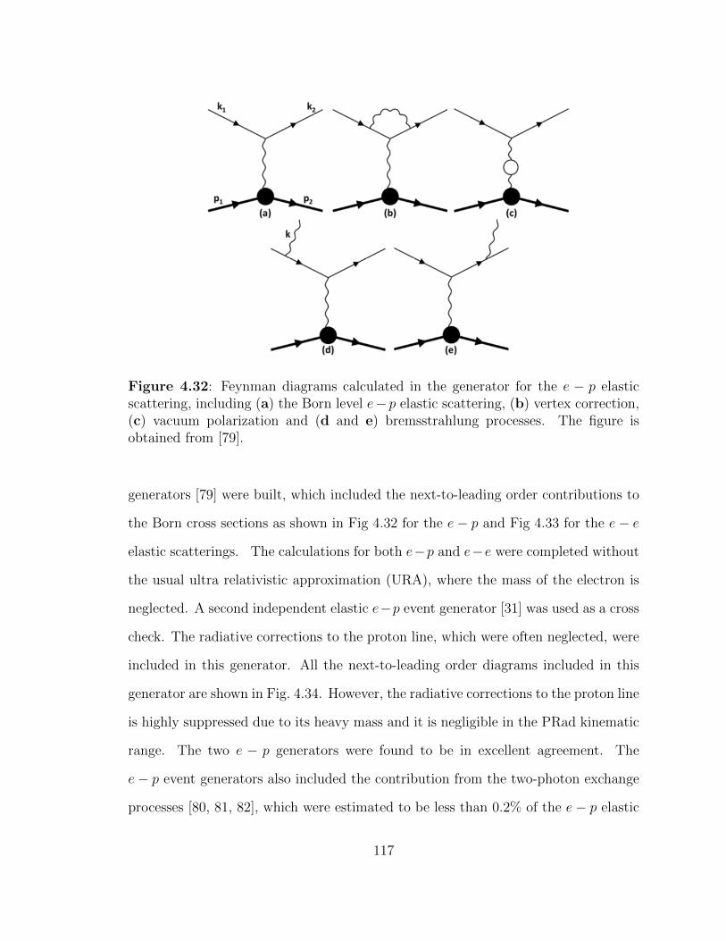
Figure 4.32: Feynman diagrams calculated in the generator for the e − p elasticscattering, including (a) the Born level e− p elastic scattering, (b) vertex correction,(c) vacuum polarization and (d and e) bremsstrahlung processes. The figure isobtained from [79].
generators [79] were built, which included the next-to-leading order contributions to
the Born cross sections as shown in Fig 4.32 for the e− p and Fig 4.33 for the e− e
elastic scatterings. The calculations for both e−p and e−e were completed without
the usual ultra relativistic approximation (URA), where the mass of the electron is
neglected. A second independent elastic e−p event generator [31] was used as a cross
check. The radiative corrections to the proton line, which were often neglected, were
included in this generator. All the next-to-leading order diagrams included in this
generator are shown in Fig. 4.34. However, the radiative corrections to the proton line
is highly suppressed due to its heavy mass and it is negligible in the PRad kinematic
range. The two e − p generators were found to be in excellent agreement. The
e− p event generators also included the contribution from the two-photon exchange
processes [80, 81, 82], which were estimated to be less than 0.2% of the e− p elastic
117

Figure 4.33: Feynman diagrams calculated in the generator for the e − e elasticscattering, including (a and b for the t and u channels, respectively) the Born levele−e elastic scattering, (c) vacuum polarization, (d and e) vertex correction, (f and g)two-photon exchange and (h to k) bremsstrahlung processes. The figure is obtainedfrom [79].
118

Figure 4.34: All the Feynman diagrams considered in Ref. [31], including (a) Bornlevel e−p elastics scattering, (b and c) bremsstrahlung radiations from the lepton line,(d and e) bremsstrahlung radiations from the proton line, (f) vacuum polarization,(g) the lepton and (h) proton vertex correction, and (i and j) box diagrams. Thefigure is obtained from Ref. [31].
scattering cross section in the PRad kinematic range. All the generators are able
to generate hard radiated photons, beyond the peaking approximation7 [83]. This is
crucial for the calorimeter simulation, as the HyCal will integrate some of the radiated
photons into the electron cluster, if they are close enough to each other when they
hit the HyCal.
The inelastic e− p scattering events were included in the simulation using an em-
pirical fit [75] to the e−p inelastic scattering world data. The inelastic e−p scattering
contributes as a background to the elastic e− p events. And the simulation was able
to reproduce the measured energy spectrum reasonably well (see section 4.5.2) once
the inelastic e− p scattering events were included.
After normalizing the integrated luminosities for the outputs of these generators,
the generated particles are then propagated in the experimental setup using the
7In the peaking approximation, the radiated photon will be co-linear with the electron.
119
Geant4 simulation. Eventually, the results are digitized into the ADC counts in the
readouts and reconstructed with the same event reconstruction algorithm as for the
data. The simulated energy spectrum is highly similar to that from the data, as
shown in Fig. 4.35.
In addition, as introduced in Section 3.3, a number of pressure gauges and tem-
perature sensors were used during the experiment to monitor the gas pressure and
temperatures at multiple locations across the entire target system. These measured
temperature values, together with the inlet gas flow rate, pumping speeds of the
vacuum pumps, and the detailed geometry of the target system were used to simu-
late the hydrogen density profile in the target using the COMSOL Multiphysics R©
simulation package. The average pressure obtained from the simulation agreed with
the measured values within 2 mTorr for both the target cell and the target chamber,
under the PRad full target running conditions. The simulated gas density profile
along the beam-line is shown in Fig. 4.36.
4.8 Angular Resolution and Q2 Resolution
Using the PRad simulation package, the polar-angle resolution of the experimental
setup can be extracted and it is shown in (a) of Fig. 4.37, for which the GEM de-
tectors were used for the (two-dimensional) position reconstruction. This resolution
is dominated by the multiple scatterings when electrons pass through external ma-
terials, in particular, the 1.6 mm thick aluminum vacuum window. The extended
target effect also plays a role, but the effect is only significant when the polar angle
is large. The polar-angle resolution is about 0.1 and 0.06 mrad at the very forward
angle, for the 1.1 and 2.2 GeV energy settings, respectively, and increases to 0.27 and
0.24 mrad at the largest angle.
120
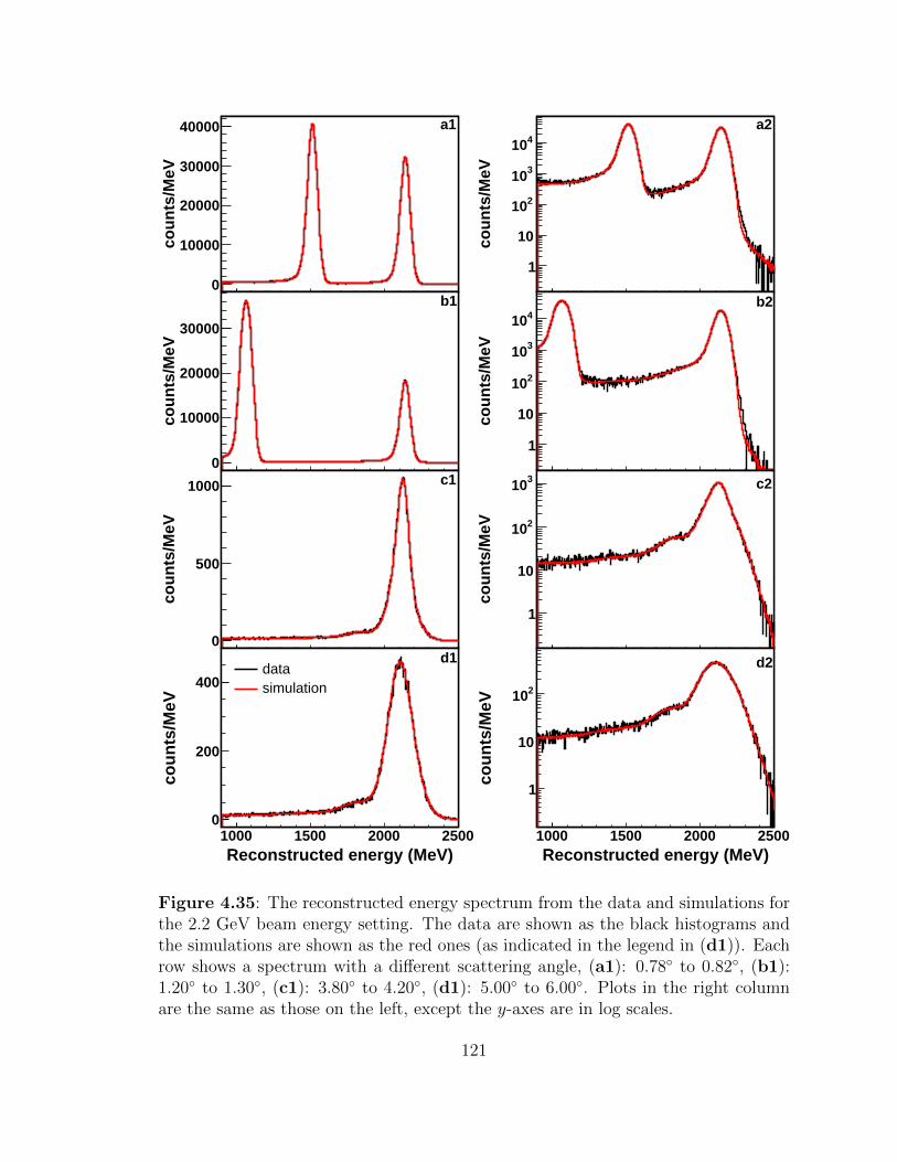
cou
nts
/MeV
0
10000
20000
30000
40000 a1
cou
nts
/MeV
0
10000
20000
30000
b1
cou
nts
/MeV
0
500
1000 c1
Reconstructed energy (MeV)1000 1500 2000 2500
cou
nts
/MeV
0
200
400
d1datasimulation
cou
nts
/MeV
1
10
210
310
410a2
cou
nts
/MeV
1
10
210
310
410b2
cou
nts
/MeV
1
10
210
310 c2
Reconstructed energy (MeV)1000 1500 2000 2500
cou
nts
/MeV
1
10
210
d2
Figure 4.35: The reconstructed energy spectrum from the data and simulations forthe 2.2 GeV beam energy setting. The data are shown as the black histograms andthe simulations are shown as the red ones (as indicated in the legend in (d1)). Eachrow shows a spectrum with a different scattering angle, (a1): 0.78 to 0.82, (b1):1.20 to 1.30, (c1): 3.80 to 4.20, (d1): 5.00 to 6.00. Plots in the right columnare the same as those on the left, except the y-axes are in log scales.
121

[cm]60- 40- 20- 0 20 40 60
]3/c
m2
Gas
den
sity
[H
1210
1310
1410
1510
1610
1710
1810COMSOL production run
COMSOL empty target run
COMSOL full target
COMSOL empty target
Figure 4.36: The simulated gas density profile along the beam line by COMSOLMultiphysics R© simulation package, for the full target run condition (black curve)and empty target run condition (red curve). The target center is placed at 0 cm inthe plot.
122
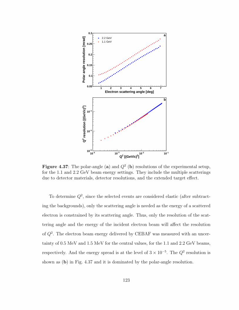
Electron scattering angle [deg]1 2 3 4 5 6 7
Po
lar
ang
le r
eso
luti
on
[m
rad
]0.05
0.1
0.15
0.2
0.25
0.3
2.2 GeV1.1 GeV
a
]2 [(GeV/c)2Q4−10 3−10 2−10 1−10
]2 r
eso
luti
on
[(G
eV/c
)2
Q
6−10
5−10
4−10
b
Figure 4.37: The polar-angle (a) and Q2 (b) resolutions of the experimental setup,for the 1.1 and 2.2 GeV beam energy settings. They include the multiple scatteringsdue to detector materials, detector resolutions, and the extended target effect.
To determine Q2, since the selected events are considered elastic (after subtract-
ing the backgrounds), only the scattering angle is needed as the energy of a scattered
electron is constrained by its scattering angle. Thus, only the resolution of the scat-
tering angle and the energy of the incident electron beam will affect the resolution
of Q2. The electron beam energy delivered by CEBAF was measured with an uncer-
tainty of 0.5 MeV and 1.5 MeV for the central values, for the 1.1 and 2.2 GeV beams,
respectively. And the energy spread is at the level of 3× 10⁻⁵. The Q2 resolution is
shown as (b) in Fig. 4.37 and it is dominated by the polar-angle resolution.
123

4.9 Cross Section Extraction
4.9.1 (e− p) /(e− e) Ratio
The e − p elastic scattering cross section is extracted based on Eq. 4.12 for the
experiment. It states that after making the efficiency corrections in both the data
and simulation, the e− p elastic scattering cross section equals to the (e− p)/(e− e)
ratio from the data over the (e− p)/(e− e) ratio from the simulation (super ratio),
multiplied by the Born e− p cross section used in the simulation.
Before obtaining the (e − p)/(e − e) ratio from the data, one needs to subtract
the e− p and e− e counts measured in the empty target runs from those in the full
target runs, after normalization by the total live charges between these two types of
runs. Due to possible fluctuations in the background rate, the entire data set was
split into smaller sub-periods (10 for the 1.1 GeV data set, and 20 for the 2.2 GeV
data set), with most of the sub-periods consisted of about 3 to 4 full target runs,
and sandwiched by two empty target runs. For an angular bin at θi, the background
subtracted e− p and e− e counts are
N e,rep (θi) =
∑j
[(N e,r
ep )full(θi)− Cj · (N e,rep )emp(θi)
], (4.29)
N e,ree (θi) =
∑j
[(N e,ree )full(θi)− Cj · (N e,r
ee )emp(θi)] . (4.30)
The subscript “full” indicates that the counts are from the full target runs, and the
subscript “emp” indicates that the counts are from empty target runs. Cj is the live
charge ratio (see Eq. 3.5) between the full target runs and the empty target runs in
the j-th sub-period, and the index j runs through all sub-periods for a beam energy
setting. After this subtraction procedure, the e−p to e−e ratio can be obtained after
124

making the detector efficiency correction to the e − p and e − e counts separately.
Other than taking the total sum of all the background subtracted counts from all the
sub-periods, one can also obtain an (e − p)/(e − e) ratio from each sub-period and
obtain the final ratio by taking a weighted average using their statistical uncertainties.
The two results differ by no more than 0.05% for all angular bins, which is negligible.
For the inelastic e− p contribution, one has the option to either subtract this in the
data or add this in the simulation. The difference in the super ratio between these
two approaches was much smaller than 0.05% for all angular bins.
For the simulation, one can obtain the (e − p)/(e − e) ratio by using the e − p,
e− e and inelastic e− p event generators and then transport the generated particles
in the Geant4 simulation. The events from these generators must be normalized to
the same integrated luminosity (the integrated luminosity of e − e in this study) as
they all share the same luminosity in the data. The exact same event selection cuts
were applied to the simulation to obtain the (e− p)/(e− e) ratio.
As mentioned at the beginning of the chapter, there are two methods to form
the e − p to e − e ratio. The first method is the bin-by-bin method, for which one
will form the ratio using the e − p and e − e counts from the same angular bin.
This method has the ability to cancel out the energy-independent part of the GEM
efficiency (see section 4.6). However, this method is limited to the angular range of
the double-arm Møller acceptance, which is significantly smaller than that for the
e−p, and it may also introduce angular-dependent systematic uncertainties from the
e−e. The other method is the integrated Møller method, which uses the e−e counts
from a selected angular range and is applied as a common normalization factor for
all angular bins of the e − p. It is applicable to all the angular bins in principle,
but requires the GEM efficiency corrections whose systematic uncertainties could be
significant especially in the forward angular region (< 1.3). However, the systematic
125

uncertainties from the e− e can only affect the normalization of the data points, and
will not affect the extracted rp. Taking various considerations into account, the range
for the bin-by-bin method is applied up to 3.0 and 1.6 for the 1.1 and 2.2 GeV data
sets, respectively. And the data points in larger angular ranges are obtained from the
integrated Møller method. The selected angular ranges for the e− e integration are
1.3 to 3.0 for the 1.1 GeV data and 1.3 to 2.0 for the 2.2 GeV data. The major
reason of choosing these ranges is that the GEM efficiency can be determined more
precisely. One can also choose some other ranges, for example 0.7 to 1.0 or 1.0 to
1.3, and the difference on the super ratio is about 0.05% compared to the default
range. The e − p to e − e super ratios obtained with both the bin-by-bin and the
integrated Møller method are very consistent in the range that they can be reliably
compared, as shown in Fig. 4.38.
The azimuthal symmetry of the super ratio between the data (e − p)/(e − e)
and the simulated (e − p)/(e − e) was studied by comparing the results obtained
from each quadrant of the HyCal calorimeter. The super ratio from each quadrant
was found to be consistent with each other within the statistical uncertainties, as
shown in Fig. 4.31 in Section 4.6. The purpose of this comparison was not only to
validate the GEM efficiency correction, but also to check the combined systematic
effects such as, the beam position, tilting angles of both the beam and detectors,
HyCal detector responses and geometric acceptances. Note that a number of these
systematic effects, such as the beam position and tilting angles of both the beam
and detectors, could be averaged out significantly when combing the data from all
the quadrants. In addition, as various properties, including the triggers, are different
between the two types of shower detectors of the HyCal, the consistency between the
PbWO4 and Pb-glass modules was also verified by comparing the super ratio with
and without using the Pb-glass modules. The super ratio in the angular range where
126

Reconstructed scattering angle [deg]1.4 1.6 1.8 2 2.2 2.4 2.6 2.8 3
sim
/(ep
/ee)
dat
a(e
p/e
e)
0.98
0.985
0.99
0.995
1
1.005
1.01
1.015
1.02Inte Moller method
Bin by bin method
a
Reconstructed scattering angle [deg]1.3 1.4 1.5 1.6 1.7 1.8 1.9 2 2.1 2.2
sim
/(ep
/ee)
dat
a(e
p/e
e)
0.98
0.985
0.99
0.995
1
1.005
1.01
1.015
1.02b
Figure 4.38: The super ratios (e − p to e − e ratios from the data over that fromthe simulation) obtained using the integrated Møller method (black solid dots) andthe bin-by-bin method (red open circle). The 1.1 GeV data are shown in (a) and2.2 GeV data are shown in (b).
127

Reconstructed scattering angle [deg]3.4 3.6 3.8 4 4.2 4.4 4.6
sim
/(ep
/ee)
dat
a(e
p/e
e)
0.97
0.98
0.99
1
1.01
1.02
1.03
4Only PbWO
All data
a
Reconstructed scattering angle [deg]3.4 3.6 3.8 4 4.2 4.4 4.6
b
Figure 4.39: The super ratio obtained when using only the PbWO4 modules andwhen using all modules for the angular region where the two types of modules haveoverlapping coverage. Plot (a) is for the 1.1 GeV and plot (b) for the 2.2 GeV electronbeam energy settings.
the two types of modules have overlapping coverage is shown in Fig. 4.39.
4.9.2 Radiative Corrections
The radiative corrections for the e− p elastic scattering cross section include the in-
ternal radiative corrections calculated by the e−p and e− e event generators [31, 79]
and the radiative correction for effects due to particles passing through external ma-
terials, which is performed by the Geant4 simulation. There are four important
parameters for the generators, including the minimum and maximum scattering an-
gles (θmin` and θmax
` ), the maximum allowed bremsstrahlung photon energy cut (Emaxγ )
and the soft photon energy cut (Eminγ ). Based on the Feynman diagrams presented in
Section. 4.7, the generators will generate all possible scattered electrons within the
angular and energy ranges defined by these four parameters, and also their associated
bremsstrahlung photons. In the ideal case if one wants to cover the full phase spaces
within the experimental kinematic range, one would generate events in the entire 4π
128
solid angle and with all possible energies for the radiated photons. However, this is
not practical computationally and the ranges for the generators have to be limited
by these parameters. They have to be chosen carefully so that the effects due to ne-
glecting events outside the ranges are negligible, and the results from the simulation
are not sensitive to the choices for these parameters. The angular range for the gen-
erators is chosen to be from 0.5 to 8.5, slightly larger than the angular acceptance
of the experimental setup. Even though events outside this range may still bounce
into the acceptance through multiple scatterings, this effect is rather negligible as
shown by the simulation. First of all, the events with smaller scattering angles will
be rejected by the matching condition between the GEMs and HyCal, as discussed
in Section 4.5.4. For the e − e events with larger scattering angles, their energies
will be too small to satisfy the event selection cuts. And for the e − p events, even
though they may still have enough energy, the cross section is decreasing drastically
with larger scattering angles. The purpose of the soft photon cut is to deal with the
infrared divergent problem of the radiated photons with very low energies, and it is
typically chosen to be much smaller than the energy resolution of the detector. For
the analysis, Eminγ = 1 MeV is used for both beam energy settings and Fig. 4.40 (a)
shows that in the case of the 1.1 GeV beam energy setting, the results with Eminγ =
2 MeV, 5 MeV and 10 MeV are consistent statistically with the one obtained with
Eminγ = 1 MeV. Similar results can be obtained from the 2.2 GeV simulation. For
Emaxγ , the difference in the simulation results becomes negligible once this cut is set
to a large enough value, such as larger than 1000 MeV for the 1.1 GeV setting, and
1800 MeV for the 2.2 GeV setting. However, the results are sensitive to this param-
eter if it is set to be too low, as shown in Fig. 4.40 (b) for the 1.1 GeV setting, in
which case the results are normalized to the one obtained with Emaxγ = 1100 MeV.
The reason is that the PRad detector setup cannot distinguish the electrons and pho-
129

Reconstructed scattering angle [deg]1 2 3 4 5 6
rati
o
0.985
0.99
0.995
1
1.005
1.01
= 2 MeVminγE
= 5 MeVminγE
= 10 MeVminγE
a
Reconstructed scattering angle [deg]1 2 3 4 5 6
rati
o
0.985
0.99
0.995
1
1.005
1.01 = 400 MeVmax
γE = 600 MeVmax
γE = 800 MeVmax
γE = 1000 MeVmax
γE
a
Figure 4.40: The elastic e − p counts from the simulation, obtained with differentEminγ (top) and Emax
γ (bottom) cuts, for the 1.1 GeV beam energy setting. The resultsin both plots are normalized to the case with Emin
γ = 1 MeV and Emaxγ = 1100 MeV.
For the top plot, Emaxγ is fixed at 1100 MeV for all the cases while for the bottom
one, Eminγ is fixed at 1 MeV for all the cases.
130

tons if they are almost co-linear. In this case, they will produce only one cluster on
the HyCal and also produce a hit on the GEMs that is able to satisfy the matching
condition. This type of events mostly come from the bremsstrahlung radiation of the
final state electrons, in which case the probability for the photon emission decreases
drastically as the photon energy increases. Thus, once this cut is large enough, the
results start to saturate. In addition, this cut mostly affects the normalization of the
results, so that the systematic uncertainty on rp is expected to be negligible once a
large cut is applied in the generators.
The radiative correction was applied using an iterative procedure, which would
replace the electric form factor used in the e−p event generator by the one extracted
from the data so that the e−p to e−e ratios between the data and simulation would
converge to unity eventually. This procedure is important also for the bin center
correction, which requires a good agreement between the simulation and the data. A
flow chart for this procedure is presented in Fig. 4.41. The Kelly form factors [84] were
used before the iteration. The super ratios before and after this iterative procedure
(4 iterations for the 1.1 GeV and 5 iterations for the 2.2 GeV data sets) are shown in
Fig. 4.42. The super ratios converged very fast after a few iterations. The differences
for the differential cross section results, before and after the iterative procedure are
shown in Fig. 4.43. The cross section results are insensitive to these cross section
models used in the simulation, as the data points are consistent statistically before
and after the iteration.
4.9.3 Born Level e− p Elastic Scattering Cross Section
The e− p elastic scattering cross sections were obtained by comparing the measured
e−p to e−e ratio to the simulated e−p to e−e ratio, as indicated by Eq. 4.12, after
the efficiency corrections for both the data and simulation. For angles below 3.0
131
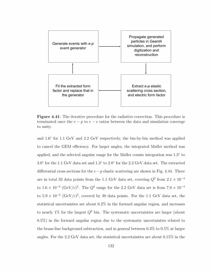
Generate events with e-pevent generator
Propagate generated particles in Geant4
simulation, and perform digitization and reconstruction
Extract e-p elastic scattering cross section, and electric form factor
Fit the extracted form factor and replace that in
the generator
Figure 4.41: The iterative procedure for the radiative correction. This procedure isterminated once the e− p to e− e ratios between the data and simulation convergeto unity.
and 1.6 for 1.1 GeV and 2.2 GeV respectively, the bin-by-bin method was applied
to cancel the GEM efficiency. For larger angles, the integrated Møller method was
applied, and the selected angular range for the Møller counts integration was 1.3 to
3.0 for the 1.1 GeV data set and 1.3 to 2.0 for the 2.2 GeV data set. The extracted
differential cross sections for the e−p elastic scattering are shown in Fig. 4.44. There
are in total 33 data points from the 1.1 GeV data set, covering Q2 from 2.1 × 10⁻⁴
to 1.6 × 10⁻² (GeV/c)2. The Q2 range for the 2.2 GeV data set is from 7.0 × 10⁻⁴
to 5.9 × 10⁻² (GeV/c)2, covered by 38 data points. For the 1.1 GeV data set, the
statistical uncertainties are about 0.2% in the forward angular region, and increases
to nearly 1% for the largest Q2 bin. The systematic uncertainties are larger (about
0.5%) in the forward angular region due to the systematic uncertainties related to
the beam-line background subtraction, and in general between 0.3% to 0.5% at larger
angles. For the 2.2 GeV data set, the statistical uncertainties are about 0.15% in the
132
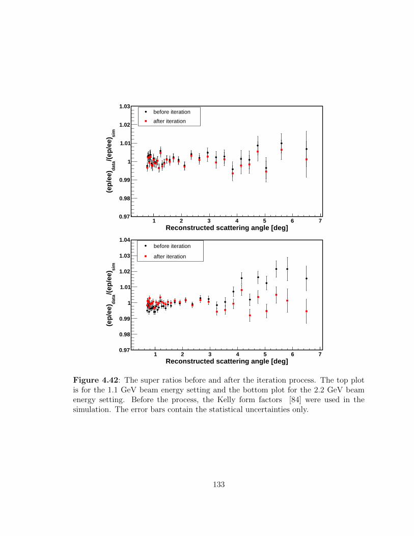
Reconstructed scattering angle [deg]1 2 3 4 5 6 7
sim
/(ep
/ee)
dat
a(e
p/e
e)
0.97
0.98
0.99
1
1.01
1.02
1.03before iteration
after iteration
Reconstructed scattering angle [deg]1 2 3 4 5 6 7
sim
/(ep
/ee)
dat
a(e
p/e
e)
0.97
0.98
0.99
1
1.01
1.02
1.03
1.04before iteration
after iteration
Figure 4.42: The super ratios before and after the iteration process. The top plotis for the 1.1 GeV beam energy setting and the bottom plot for the 2.2 GeV beamenergy setting. Before the process, the Kelly form factors [84] were used in thesimulation. The error bars contain the statistical uncertainties only.
133
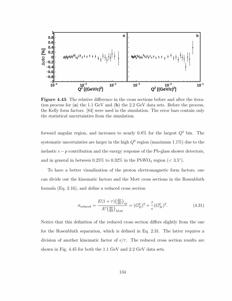
]2 [(GeV/c)2Q4−10 3−10 2−10
[%
]σ/σ∆
1−0.8−0.6−0.4−0.2−
00.20.40.60.8
1a
]2 [(GeV/c)2Q3−10 2−10 1−10
[%
]σ/σ∆
1−0.8−0.6−0.4−0.2−
00.20.40.60.8
1b
Figure 4.43: The relative difference in the cross sections before and after the itera-tion process for (a) the 1.1 GeV and (b) the 2.2 GeV data sets. Before the process,the Kelly form factors [84] were used in the simulation. The error bars contain onlythe statistical uncertainties from the simulation.
forward angular region, and increases to nearly 0.8% for the largest Q2 bin. The
systematic uncertainties are larger in the high Q2 region (maximum 1.1%) due to the
inelastic e−p contribution and the energy response of the Pb-glass shower detectors,
and in general in between 0.25% to 0.32% in the PbWO4 region (< 3.5).
To have a better visualization of the proton electromagnetic form factors, one
can divide out the kinematic factors and the Mott cross sections in the Rosenbluth
formula (Eq. 2.16), and define a reduced cross section
σreduced =E(1 + τ)
(dσdΩ
)ep
E ′(dσdΩ
)Mott
= (GpE)2 +
τ
ε(Gp
M)2. (4.31)
Notice that this definition of the reduced cross section differs slightly from the one
for the Rosenbluth separation, which is defined in Eq. 2.31. The latter requires a
division of another kinematic factor of ε/τ . The reduced cross section results are
shown in Fig. 4.45 for both the 1.1 GeV and 2.2 GeV data sets.
134

]2 [(GeV/c)2Q3−10 2−10
[m
b/s
r]ep
→ep
Ω/dσd
3−10
2−10
1−10
1
10
210
310a
]2 [(GeV/c)2Q3−10 2−10 1−10
3−10
2−10
1−10
1
10
210
310b
Stat. Uncertainty (right axis)
Syst. Uncertainty (right axis)012012
012
[%]
012
Figure 4.44: The Born level differential cross sections for the e−p elastic scatteringfrom (a) the 1.1 GeV and (b) the 2.2 GeV data sets. Statistical and systematicuncertainties are shown as separate bands and are scaled to the right axes of eachplot.
Figure 4.45: The reduced cross section as defined in Eq. 4.31, for the 1.1 GeV and2.2 GeV data sets. After dividing out the kinematic factors, the reduced cross sectionis a linear combination of the electromagnetic form factors squared.
135
4.10 Systematic Uncertainties on Cross Section
The systematic uncertainties of the PRad experiment are grouped into uncorrelated
uncertainties and correlated ones. The latter are further divided into normalization
uncertainties and Q2-dependent uncertainties. Only a few systematic uncertainties
may be considered uncorrelated, that is, no clear correlations are observed among
different angular or Q2 bins. These include the uncertainties in the detector effi-
ciency measurements, parts of the energy calibration of the HyCal modules, and also
parts of the detector responses for the Pb-glass detectors. Unlike the PbWO4 mod-
ules, which show clear similarities, the Pb-glass modules have some differences in
their responses and no clear correlations are observed among them. So, these sys-
tematic uncertainties are assumed to be uncorrelated. Most of the other systematic
uncertainties are considered to be correlated, and their angular dependencies are ex-
tracted using either the data or the simulation, and are included in the systematic
uncertainty studies. A few items, such as the energy cuts in the event selection, and
the time-stability of the background subtraction are considered to be mixed, that is,
they are partially correlated and partially uncorrelated. Studies for their systematic
uncertainties involve using many different sizes for the event selection cuts and us-
ing different combinations of empty target runs to do the background subtraction.
All the systematic uncertainties that are considered for the cross section results are
shown in the following list:
1. Event selection
2. Detector efficiency
3. Beam-line background
4. HyCal response
136
5. Geometric acceptance
6. Beam energy
7. Energy loss and multiple scattering due to external materials
8. Radiative corrections for e− p and e− e
9. Inelastic e− p
The total relative systematic uncertainties for the cross sections are shown in Fig. 4.46
for both the 1.1 and 2.2 GeV data sets. The first item is related to various cuts used
to select the e − p and e − e elastic scattering events, which will be discussed in
the Sub-section 4.10.1. Various systematic uncertainties can arise from the imperfect
knowledge about the experimental setup, such as the beam energy, positions and
efficiencies of the detectors, the HyCal energy response to incident particles, and
fluctuations and possible biases in the beam-line background subtraction. These
are related to various conditions while the experiment was taking place and they
will be discussed in the Sub-section 4.10.2. Lastly, the cross section results depend
inevitably on certain models and calculations, such as the radiative corrections for
the e − p and e − e and also the inelastic e − p subtraction. They are discussed in
the Sub-section 4.10.3.
4.10.1 Systematic Uncertainties Associated with Cuts
A series of cuts were used in the analysis to select the elastic e−p and e−e events, such
as the kinematic cuts for both reaction channels, and the coplanarity and vertex-z
cuts for the e−e events. Slightly different cross sections results can be obtained once
the sizes of these cuts are changed, and this variation arises from the fact that there
are always some slight differences between the data and simulation. For example, for
137

Reconstructed scattering angle [deg]1 2 3 4 5 6 7
Rel
ativ
e u
nce
rtai
nty
[%
]
0
0.2
0.4
0.6
0.8
1
1.2
1.4 1GeV
2GeV
Figure 4.46: Total relative systematic uncertainties for the e− p elastic scatteringcross sections for the 1.1 and 2.2 GeV data sets.
the shape of the elastic e − p peak, the central positions and widths obtained from
the data and simulation match very well, however, there can be small differences in
the tail regions (see Fig. 4.35). These differences may arise from various sources such
as the light attenuation in the modules, the non-linearity, the gaps between HyCal
modules that are not simulated perfectly, other electronics related effects that were
unaccounted for in the detector digitization and so on. These sources are typically
very difficult to be isolated and studied separately. In order to quantify their overall
effects, the sizes of the event selection cuts are varied around the nominal cuts used
to obtain the cross section results (see Table 4.3 and Table 4.4). The root-mean-
squares (RMS) of the cross section results as one changes these cuts are used as the
uncertainties due to the event selection.
The uncertainties for the event selection are dominated by those cuts related to
the HyCal reconstructed energy, such as the kinematic cuts. And the variations
138
are not uniform across different detector modules of the HyCal, especially given
that it consists of two different types of shower detectors. These variations may
come from small inter-module differences in properties such as the light attenuation,
non-linearity of detector responses, microscopic gaps between detector modules and
the energy calibrations. The effect of this systematic uncertainty was studied by
varying the kinematic cuts over a wide range, which is ± 20% for the 1.1 GeV
default kinematic cuts and at least ± 50% for the 2.2 GeV default kinematic cuts
(see Table 4.3 and Table 4.4). The reason of a smaller range for the 1.1 GeV data
set is because the e− p and e− e elastic peaks are very close, particularly in the very
forward angular region (< 1.0 for instance). Increasing the cut size for the e − p
events can include significant amount of e− e events and vice versa.
The super ratios (proportional to the cross section) as a function of the e − p
kinematic cut size, are shown in Fig 4.47 and Fig 4.48. The variation of the kinematic
cut leads to changes in the extracted cross section of about 0.1%, on average, and
is typically within ± 0.15%, except for the last few bins in the large angular region.
This is most likely due to the lack of statistics in the fine tuning process of the
energy calibrations for the Pb-glass modules and the effect is more significant if the
size of the kinematic cut is reduced. In the PbWO4 region (< 3.4), the variation
is significantly smaller and it is most likely due to the light attenuation property
of the PbWO4 modules and the gaps between them. The variations when changing
the energy cuts for the e− e (see Fig 4.49 and Fig 4.50) are typically slightly larger
than those for the e − p in the similar detector region. This is because the double-
arm Møller selection requires three cuts on the HyCal reconstructed energy for each
event (two kinematic cuts for the two scattered electrons and an elasticity cut for
the total energy of these two electrons). However, the variation is more uniform
139
across the HyCal8, which means varying energy cuts for the e−e mostly just changes
the normalization of the data points and the angular dependency of the variation is
significantly smaller than that for the e−p. The RMSs of the cross section results, due
to the change in the size of the energy cuts, are used as the systematic uncertainty.
For the co-planarity and vertex-z cuts, the variations are negligible compared to
those from the energy cuts. Only a 0.02% difference was observed when changing
the sizes of these cuts by ±20%, and the difference is mostly on the normalization
of the data points. The cross section results are also shown to be insensitive to the
matching cuts between the GEMs and HyCal. The default value for this cut is 6σ
of the HyCal position resolution. When using 5σ, 7σ and 8σ cuts, the RMSs of the
cross section results are about 0.02% (mostly uncorrelated) of the nominal ones. The
sensitivity on the selected angular ranges for the integrated Møller method was also
included for the systematic uncertainties of the event selection. These ranges are, by
default, 1.3 to 3.0 for the 1.1 GeV data set and 1.3 to 2.0 for the 2.2 GeV data set,
as the GEM efficiency could be more precisely determined in these ranges. Typically
around 0.05% difference would appear if some other ranges are used, such as 0.7
to 1.0 or 1.0 to 1.3. This difference is assigned as the corresponding systematic
uncertainty.
4.10.2 Systematic uncertainties from Experimental Conditions
Detector efficiency: These systematic uncertainties include two items. The first item
includes the statistical uncertainties in the detector efficiency measurements, namely,
measurements of the HyCal trigger efficiency and the GEM efficiency. These statis-
tical uncertainties are determined using the Binomial distribution. For the HyCal
trigger efficiency, the uncertainties are typically less than 0.03% for each module, so
8Partially because the double-arm Møllers are mostly inside the PbWO4 detector region.
140

Multiplication factor0.8 0.9 1 1.1 1.2
sim
/(ep
/ee)
dat
a(e
p/e
e)
0.995
1
1.005o < 0.825θ < o0.800
Multiplication factor0.8 0.9 1 1.1 1.2
sim
/(ep
/ee)
dat
a(e
p/e
e)
0.995
1
1.005o < 1.211θ < o1.157
Multiplication factor0.8 0.9 1 1.1 1.2
sim
/(ep
/ee)
dat
a(e
p/e
e)
0.995
1
1.005o < 2.000θ < o1.787
Multiplication factor0.8 0.9 1 1.1 1.2
sim
/(ep
/ee)
dat
a(e
p/e
e)0.995
1
1.005o < 2.792θ < o2.492
Multiplication factor0.8 0.9 1 1.1 1.2
sim
/(ep
/ee)
dat
a(e
p/e
e)
0.99
1
1.01 o < 3.692θ < o3.392
Multiplication factor0.8 0.9 1 1.1 1.2
sim
/(ep
/ee)
dat
a(e
p/e
e)
0.99
1
1.01 o < 4.592θ < o4.292
Multiplication factor0.8 0.9 1 1.1 1.2
sim
/(ep
/ee)
dat
a(e
p/e
e)
0.98
0.99
1
1.01
1.02 o < 5.200θ < o4.892
Multiplication factor0.8 0.9 1 1.1 1.2
sim
/(ep
/ee)
dat
a(e
p/e
e)
0.98
0.99
1
1.01
1.02 o < 7.000θ < o6.000
Figure 4.47: The variations of the super ratio results when changing the size of thekinematic cuts for the 1.1 GeV e− p event selection, for different scattering angularbins. The multiplication factor is to be multiplied on top of the default sizes of thekinematic cuts, listed in Table 4.3. A multiplication factor of 0.8 means reducingthe sizes by 20%, which leads to -2.40 σdet to 2.40 σdet for the size of the cut in thePbWO4 region for instance. Data points are shifted so that the super ratio with thedefault cut size is at unity.
141
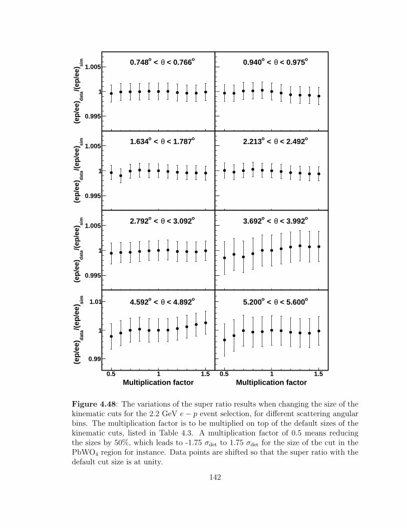
Multiplication factor0.5 1 1.5
sim
/(ep
/ee)
dat
a(e
p/e
e)
0.995
1
1.005o < 0.766θ < o0.748
Multiplication factor0.5 1 1.5
sim
/(ep
/ee)
dat
a(e
p/e
e)
0.995
1
1.005o < 0.975θ < o0.940
Multiplication factor0.5 1 1.5
sim
/(ep
/ee)
dat
a(e
p/e
e)
0.995
1
1.005o < 1.787θ < o1.634
Multiplication factor0.5 1 1.5
sim
/(ep
/ee)
dat
a(e
p/e
e)0.995
1
1.005o < 2.492θ < o2.213
Multiplication factor0.5 1 1.5
sim
/(ep
/ee)
dat
a(e
p/e
e)
0.995
1
1.005o < 3.092θ < o2.792
Multiplication factor0.5 1 1.5
sim
/(ep
/ee)
dat
a(e
p/e
e)
0.995
1
1.005o < 3.992θ < o3.692
Multiplication factor0.5 1 1.5
sim
/(ep
/ee)
dat
a(e
p/e
e)
0.99
1
1.01 o < 4.892θ < o4.592
Multiplication factor0.5 1 1.5
sim
/(ep
/ee)
dat
a(e
p/e
e)
0.99
1
1.01 o < 5.600θ < o5.200
Figure 4.48: The variations of the super ratio results when changing the size of thekinematic cuts for the 2.2 GeV e− p event selection, for different scattering angularbins. The multiplication factor is to be multiplied on top of the default sizes of thekinematic cuts, listed in Table 4.3. A multiplication factor of 0.5 means reducingthe sizes by 50%, which leads to -1.75 σdet to 1.75 σdet for the size of the cut in thePbWO4 region for instance. Data points are shifted so that the super ratio with thedefault cut size is at unity.
142

Multiplication factor0.8 0.9 1 1.1 1.2
sim
/(ep
/ee)
dat
a(e
p/e
e)
0.995
1
1.005o < 0.825θ < o0.800
Multiplication factor0.8 0.9 1 1.1 1.2
sim
/(ep
/ee)
dat
a(e
p/e
e)0.995
1
1.005o < 1.211θ < o1.157
Multiplication factor0.8 0.9 1 1.1 1.2
sim
/(ep
/ee)
dat
a(e
p/e
e)
0.995
1
1.005o < 1.634θ < o1.514
Multiplication factor0.8 0.9 1 1.1 1.2
sim
/(ep
/ee)
dat
a(e
p/e
e)
0.995
1
1.005o < 2.792θ < o2.492
Figure 4.49: The variations of the super ratio results when changing the size ofthe energy cuts for the 1.1 GeV e− e event selection, for different scattering angularbins. The multiplication factor is to be multiplied on top of the default sizes of thekinematic cuts, listed in Table 4.4. A multiplication factor of 0.8 means reducingthe sizes by 20%, which leads to -2.40 σdet to 2.40 σdet for the size of the cut in thePbWO4 region for instance. Data points are shifted so that the super ratio with thedefault cut size is at unity.
143
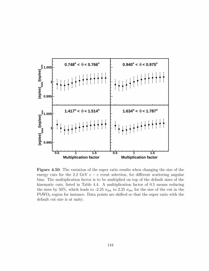
Multiplication factor0.5 1 1.5
sim
/(ep
/ee)
dat
a(e
p/e
e)
0.995
1
1.005o < 0.766θ < o0.748
Multiplication factor0.5 1 1.5
sim
/(ep
/ee)
dat
a(e
p/e
e)0.995
1
1.005o < 0.975θ < o0.940
Multiplication factor0.5 1 1.5
sim
/(ep
/ee)
dat
a(e
p/e
e)
0.995
1
1.005o < 1.514θ < o1.417
Multiplication factor0.5 1 1.5
sim
/(ep
/ee)
dat
a(e
p/e
e)
0.995
1
1.005o < 1.787θ < o1.634
Figure 4.50: The variation of the super ratio results when changing the size of theenergy cuts for the 2.2 GeV e − e event selection, for different scattering angularbins. The multiplication factor is to be multiplied on top of the default sizes of thekinematic cuts, listed in Table 4.4. A multiplication factor of 0.5 means reducingthe sizes by 50%, which leads to -2.25 σdet to 2.25 σdet for the size of the cut in thePbWO4 region for instance. Data points are shifted so that the super ratio with thedefault cut size is at unity.
144

the effect is negligible. For the statistical uncertainties of the GEM efficiency, only
data points obtained using the integrated Møller method can be affected (scattering
angles larger than 3.0 for 1.1 GeV and 1.6 for 2.2 GeV data sets), as the GEM
efficiency correction is not needed for the bin-by-bin method. For the 2.2 GeV data
set, this uncertainty is about 0.05% at 1.6 and increases to 0.3% for the largest
angular bin. For the 1.1 GeV data set, it is about 0.1% at 3.0 and increases to
0.4% for the largest angular bin. These statistical uncertainties should be considered
uncorrelated among different angular bins. The second item includes the uncertain-
ties in the GEM efficiency measurements due to the finite HyCal position resolution
effect (see Section 4.6). The uncertainties from this source are estimated by running
multiple simulations with slightly different widths and locations for the GEM spac-
ers, and then compared the GEM efficiency corrected cross section results to those
obtained with perfect GEMs (no GEM spacers and other dead areas). These simula-
tions include ± 0.9 mm variations around the nominal width (3.0 mm) and ± 2 mm
variations around the measured locations for the GEM spacers. This source can in-
troduce a maximum uncertainty of 0.35% on the 1.1 GeV cross sections and 0.25%
on the 2.2 GeV cross sections. The background related systematic uncertainties for
the GEM efficiency, such as those due to cosmic events, high energy photons and
very-small-angle-scattering events (see Section 4.5.4 and Section 4.6) are considered
negligible.
Beam-line background: There are three items included in the systematic uncer-
tainties due to the beam-line background subtraction. The first one is the time
variation of the background, which was studied by performing the background sub-
traction using different combinations of the empty target runs, such as, the empty
target run before or after the corresponding production runs, or the average of these
two empty target runs. The RMSs of the cross sections were used as the systematic
145

uncertainties due to the time variation of the background subtraction. These uncer-
tainties are negligible for the 2.2 GeV cross section results (∼ 0.02%) as the beam-line
background was highly stable during the experiment, but is one of the dominant un-
certainties for the 1.1 GeV data set. It introduces nearly 0.5% uncertainties on the
cross sections in the very forward angular region, and reduces to around 0.25% for
larger angles. The second item is the uncertainty in the live charge measurement,
and the nominal uncertainty is about 0.1%. This leads to a maximum 0.05% and
0.02% uncertainties on the cross sections below 1.1 for the 1.1 and 2.2 GeV data
sets, respectively, as the background rates are high in this region. The last item is
related to the background hydrogen gas distribution around the target cell. When
the hydrogen gas is filled directly into the target cell, it produces two diffusing tails
as it exits the window-less cell through the orifices. The empty target runs can only
be used to subtract hydrogen gas that is far away from the cell and cannot reproduce
these tails, as the gas is filled directly into the chamber. In this case, effects due to
these tails can cause systematic uncertainties for the results. One way to quantify this
effect is to study the vertex-z distributions in the data and simulation, reconstructed
by two hits on the GEMs from the double arm Møller events. Over 10 different gas
profiles were used to study the comparisons of the vertex-z distributions between the
data and simulation, and also to study the effects on the cross section results. They
include gas profiles from the COMSOL simulation and a number of variations based
on that, no gas outside the target cell, and profiles based on a simple gas diffusion
relation 1/(dz + c)2, where dz is the z−coordinate difference between a point outside
the cell and the orifice, and c is a tunable parameter that can control the size of
the diffusing tails. To estimate the possible systematic uncertainties, we use the two
extreme cases. In the first case (min. tails), the gas profile has no diffusing tails out-
side the target cell. The vertex-z distribution simulated with this profile always gives
146
smaller tails compared to the same distribution from the data, as shown in Fig. 4.51
for the 2.2 GeV setting. In the second case (max. tails), we use one of the gas profiles
based on the simple gas diffusion model, which always gives larger tails compared to
the same distribution from the data. The ratios between the e − p to e − e ratios,
obtained with these two gas profiles, are shown in Fig. 4.52 for the 2.2 GeV setting.
The effect on the cross section results is correlated. The e−p to e−e ratios obtained
in the second case are larger than those in the first case by around 0.2% for the very
forward angles, and then converge almost linearly with larger angles. This effect is
about the same for the 1.1 GeV setting. The differences in the results obtained with
these two gas profiles are used as the 3σ boundaries for the systematic uncertainties
due to the diffusing gas tails.
HyCal response: This item is mainly related to the HyCal energy response for an
incident particle with different energies (non-linearity). There are a number of fac-
tors that can affect the nonlinear behavior of a module, such as the light attenuation,
pedestal cuts, back scattering of secondary particles and so on. A typical nonlinear
behavior of a HyCal module is shown in Fig. 4.10 over a very broad energy range
of an incident particle, based on measurements from the PrimEx-II experiment [65].
The linearity is usually very good when the energy of the incident particle is high, but
changes rapidly at the low energy side mainly due to the pedestal cuts. For the PRad
experiment, the non-linearity near the elastic e− p peak can be measured using the
data from production runs if the energies of the scattered electrons from both e− p
and e− e scatterings are high enough, so that they are both on the linear part of the
response curve. This is true for most of the PbWO4 modules and some of the Pb-glass
modules that are covering smaller scattering angles. However, when the scattering
angles are too large, the incident energies of the e − e electrons become so low that
they will fall on the rapidly changing part of the response curve, and it can no longer
147

[mm]target - zrecz200− 150− 100− 50− 0 50 100 150 200
cou
nts
/mm
0
10
20
30
40
50
60
70
80
310×datamin. tailsmax. tails
[mm]target - zrecz200− 150− 100− 50− 0 50 100 150 200
cou
nts
/mm
0
2
4
6
8
10310×
datamin. tailsmax. tails
Figure 4.51: The z-vertex distributions from the 2.2 GeV data (black histogram),and simulations using the gas profiles with min. tails (green histogram) and max.tails (red histogram). All distributions are normalized by the integrals in the peakregion (from -20 mm to 20 mm, size of the target cell). The bottom plot is a zoom-in ofthe top plot. The distribution from the data is completely within the two boundariesset by the simulations with min. and max. tails.
148

Reconstructed scattering angle [deg]1 2 3 4 5 6 7
min
.si
m/(
ep/e
e)m
ax.
sim
(ep
/ee)
0.996
0.998
1
1.002
1.004
1.006
1.008
1.01 / ndf 2χ 15.62 / 18
Prob 0.6189p0 0.0001967± 1.002 p1 0.0001253±0.000346 −
/ ndf 2χ 15.62 / 18Prob 0.6189p0 0.0001967± 1.002 p1 0.0001253±0.000346 −
Figure 4.52: The e− p to e− e ratios obtained with the gas profile with max. tailsover those with the min. tails, in the case of the 2.2 GeV energy setting. The redsolid line is a linear fit to the super ratios.
149

be used to measure the non-linearity near the e − p peak. Thus, the uncertainty
associated with non-linearity corrections primarily affects data points in the large
angular region and it is expected to be larger for the 2.2 GeV setting as the HyCal
gain was lower and the effect due to the pedestal cuts would be more significant. In
addition, for the 2.2 GeV data set, these corrections affect directly the position of the
∆-resonance peak, which is significantly larger than that in the 1.1 GeV data set. To
estimate these uncertainties, a few versions of the non-linearity corrections are used
for modules in the large angular region, including those from the PrimEx-II exper-
iment and those that can produce the best match for the ∆-resonance peak in the
data and simulation. For the 2.2 GeV setting, the uncertainties are mostly correlated
and are estimated to be negligible in the PbWO4 region (< 3.4) but increase linearly
to about 1% at the largest angular bin. Additional uncorrelated uncertainties are as-
signed in order to take into account the module-by-module differences in the Pb-glass
nonlinear properties. These systematic uncertainties are negligible at 3.4 and grow
linearly to 0.4% at the largest angular bin. On the other hand, for the 1.1 GeV data
set, the differences between results obtained with different non-linearity corrections
are much smaller than the statistical uncertainties of the data points and the effect
is expected to be negligible. The other item considered for the HyCal response is
the non-uniformity correction for the HyCal energy reconstruction (discussed in sec-
tion 4.3.1). In principle, to extract this correction, one will need to study the ratio
(Erec/Eexp) as a function of the reconstructed position for each module separately.
This is particularly important for the Pb-glass modules as their non-uniformities are
very different from each other. This requires a sufficient amount of statistics from
the production runs for each module. However, the e− p cross section drops drasti-
cally at large scattering angles, and one has to group multiple neighboring modules
in order to extract this correction. And one has to assume that the correction is
150

applicable to all modules within the group, which makes this correction much less
reliable compared to that for the PbWO4 modules. The systematic uncertainties
are expected to be larger for the 2.2 GeV data set, as the non-uniformity effect is
relatively larger than that for the 1.1 GeV data and a tighter energy cut is used in
order to reject inelastic e−p events. Given that no clear correlations are observed for
this non-uniformity behavior among the Pb-glass modules, uncorrelated systematic
uncertainties are assigned for the 2.2 GeV data points in the large angular region.
The sizes of these uncertainties are considered negligible at 3.4 and increase linearly
to 0.3% at the largest angular bin.
Beam energy: The measured beam energy for the 1.1 GeV data set is 1101.0 MeV
± 0.5 MeV, and 2143.0 MeV ± 1.5 MeV for the 2.2 GeV data set. These uncertain-
ties are assumed to be Gaussian distributed, with the widths equal to 0.5 MeV and
1.5 MeV for the 1.1 and 2.2 GeV data sets, respectively. The effects due to these
systematic uncertainties are determined by running multiple simulations with dif-
ferent beam energies. Ratios between the e − p to e − e ratios with different beam
energies and those obtained with the nominal beam energy, are shown in Fig 4.53
for the 2.2 GeV beam energy setting. Note that as the z positions of the detectors
were determined using Eq. 4.23 (see Section 4.3.2), which depend also on the beam
energy. Thus, there is a strong correlation between the beam energy and detector z
positions. That is, for every 1 MeV increase in the beam energy, it corresponds to
a 2.3 mm shift in z for the 1.1 GeV energy setting, and a 1.2 mm shift in z for the
2.2 GeV energy setting, as shown in Fig. 4.54. Therefore, the systematic uncertain-
ties for the beam energy will include the beam-energy-dependent part of the detector
position systematic uncertainties. In fact, these two systematic effects will partially
cancel out each other due to this correlation. The total systematic uncertainties on
the cross sections due to the beam energy are about 0.1% for the 2.2 GeV data set
151
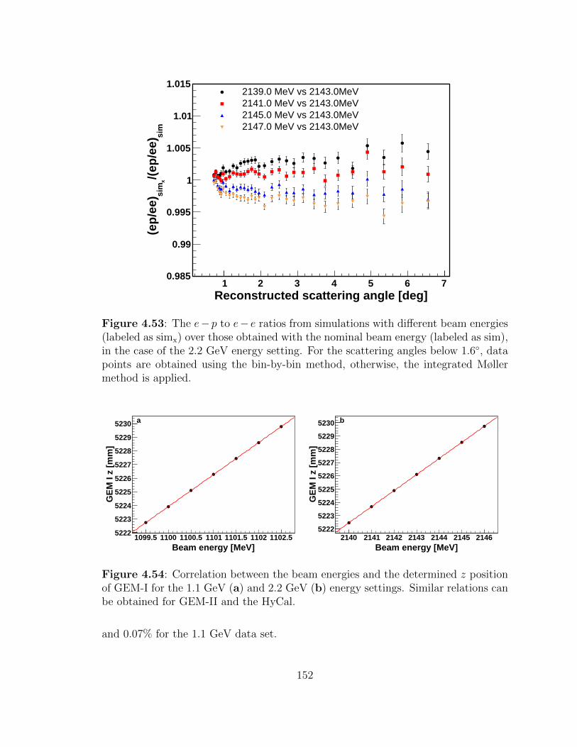
Reconstructed scattering angle [deg]1 2 3 4 5 6 7
sim
/(ep
/ee)
xsi
m(e
p/e
e)
0.985
0.99
0.995
1
1.005
1.01
1.0152139.0 MeV vs 2143.0MeV2141.0 MeV vs 2143.0MeV2145.0 MeV vs 2143.0MeV2147.0 MeV vs 2143.0MeV
Figure 4.53: The e− p to e− e ratios from simulations with different beam energies(labeled as simx) over those obtained with the nominal beam energy (labeled as sim),in the case of the 2.2 GeV energy setting. For the scattering angles below 1.6, datapoints are obtained using the bin-by-bin method, otherwise, the integrated Møllermethod is applied.
Beam energy [MeV]1099.5 1100 1100.5 1101 1101.5 1102 1102.5
GE
M I
z [m
m]
5222
5223
5224
5225
5226
5227
5228
5229
5230 a
Beam energy [MeV]2140 2141 2142 2143 2144 2145 2146
GE
M I
z [m
m]
5222
5223
5224
5225
5226
5227
5228
5229
5230 b
Figure 4.54: Correlation between the beam energies and the determined z positionof GEM-I for the 1.1 GeV (a) and 2.2 GeV (b) energy settings. Similar relations canbe obtained for GEM-II and the HyCal.
and 0.07% for the 1.1 GeV data set.
152

Geometric acceptance: this item includes the uncertainties in the detector posi-
tions, beam position, dead module removal cuts for certain HyCal modules (due to low
trigger efficiency and no ADC readout), and microscopic gaps between the modules.
For the detector positions of the GEMs, the beam-energy-dependent part is included
in the systematic uncertainties due to the beam energy. The energy-independent part
may come from the statistical uncertainties in the selected double-arm Møller events,
the uncertainties in the beam position and so on. It is assumed to be around 1 mm,
since the determined values for the detector positions using data from the production
runs (see Table 4.2) and the surveyed results agree at this level. The effects on the
cross section results are determined by running a number of simulations with slightly
different GEM positions, varied around the measured positions based on a Gaus-
sian distribution with 1 mm width. For data points obtained using the integrated
Møller method, the shifts in the GEM positions mostly just affect the normalization
of the data points, at around ± 0.05%. For data points obtained using the bin-by-bin
method, it starts from nearly 0 at the most forward angle and then increases to about
0.05% at around 3.0 and 1.6 for the 1.1 and 2.2 GeV data set, respectively. The e−p
to e−e ratios from a few versions of these simulations versus those obtained from the
standard simulation are shown in Fig 4.55. The Q2-dependent uncertainty mostly
comes from the Møller through the bin-by-bin method. For the HyCal position, the
effect is rather negligible since the HyCal reconstructed coordinates are eventually
replaced by the GEM coordinates after matching. The tilting angles of the detectors
were surveyed by the Jefferson Lab survey group before the experiment took place.
The maximum tilting angle of all the detectors is about 0.016. The effect will very
likely get averaged out (at least partially) by combining the data from the full 2π
azimuthal angle. The systematic uncertainties are studied using the simulation and
found to be negligible. Similarly, for the systematic uncertainties due to the beam
153

position, the effect will get averaged out by using the data from the full 2π azimuthal
angle, and it is also shown to be negligible. There were in total 3 PbWO4 and 4 Pb-
glass dead modules in the HyCal and they needed to be removed during the analysis.
The cut to remove a dead module would remove all the hits reconstructed inside a
circle around the center of a dead modules, with the radius as 1.5 times the size of
the module (20.75mm for a PbWO4 and 38.15mm for a Pb-glass module). These
cuts are varied from 1 to 2 times the size of the module and the RMSs of the cross
sections are assigned as the associated systematic uncertainties. There should be no
need to use a larger cut size since the lateral shower width is very narrow in the
HyCal. On average nearly 80% of the energy deposition is in the central module of
a cluster. Apparently, only angular bins containing dead modules would be affected,
and it is at maximum 0.14% for the 1.1 GeV cross sections and 0.11% for the 2.2 GeV
cross sections, at around 3.9 where there were two low efficiency Pb-glass modules
removed during the analysis. For the microscopic gaps between the modules, the
systematic uncertainties are studied by randomly varying the sizes of the PbWO4
modules by 20 µm and 100 µm for the Pb-glass modules in the simulation, and then
comparing the results to those obtained with standard sizes. The observed variations
are a few times smaller than the statistical uncertainties of the cross section results,
and they are uncorrelated. Thus, this effect should be rather negligible.
Energy loss and multiple scattering due to external materials: radiative effects
such as the bremsstrahlung radiation, ionization energy loss and also multiple scat-
tering are simulated by Geant4 as particles propagate inside the experimental setup.
They depend on the geometric and material information in the simulation about
these external materials, and also the physics list used in the simulation for com-
puting these effects. They may cause systematic uncertainties in the results as they
may not reflect exactly the reality. These systematic uncertainties are studied by
154

Reconstructed scattering angle [deg]0 1 2 3 4 5 6 7
sim
/(ep
/ee)
xsi
m(e
p/e
e)
0.995
0.996
0.997
0.998
0.999
1
1.001
1.002
1.003
1.004
1.005GEM shift -2.0 mmGEM shift -1.0 mmGEM shift 1.0 mmGEM shift 2.0 mm
Reconstructed scattering angle [deg]0 1 2 3 4 5 6 7
sim
/(ep
/ee)
xsi
m(e
p/e
e)
0.995
0.996
0.997
0.998
0.999
1
1.001
1.002
1.003
1.004
1.005GEM shift -2.0 mmGEM shift -1.0 mmGEM shift 1.0 mmGEM shift 2.0 mm
Figure 4.55: The e − p to e − e ratios from different simulations (labeled as simx)with shifted GEM positions (positive shift means shift to down stream) over thoseobtained from the standard simulation (labeled as sim), for the 1.1 GeV (top) and2.2 GeV (bottom) energy settings.
155
changing the areal densities of the external materials between the target and HyCal
by ±20%, shifting the positions for some of the dominant sources of radiative effects
(the aluminum vacuum window for instance), and also changing the physics list used
in the simulation. The observed deviation from the default simulation is mostly on
the normalization of the data points. In order words, these radiative effects due to
external materials mostly shift all data points in the same way and no clear angu-
lar dependency was observed. A systematic uncertainty of 0.2% is assigned for this
source.
4.10.3 Systematic uncertainties from Models
Internal radiative corrections for the e − p and e − e: The systematic uncertain-
ties due to the radiative corrections arise mainly from higher order contributions to
the cross sections for both elastic e − p and e − e scatterings. The next-to-leading
order diagrams (see Fig. 4.32 and Fig. 4.33) are calculated exactly beyond the ultra-
relativistic approximation [79] and included in the analysis. These corrections also
include the multi-photon emission and multi-loop processes, which are approximated
at the Q2 → 0 limit by the exponentiation procedure described in Ref. [79]. How-
ever, these higher order contributions are not calculated exactly, and the possible
systematic uncertainties are estimated based on the approach by Arbuzov and Kopy-
lova [85], for some of the higher order radiative corrections. The estimated systematic
uncertainties for both the e−p and Møller are correlated and Q2-dependent [86]. The
estimated systematic uncertainties on the cross sections are shown in Fig. 4.56 for
the 1.1 GeV and 2.2 GeV data sets. The Q2-dependence is larger for the Møller
and it affects the cross section results through the use of the bin-by-bin method.
This can be seen from the uncertainties below 1.6 for the 2.2 GeV and 3.0 for
the 1.1 GeV where the bin-by-bin method is applied. On the other hand, the Q2-
156

Reconstructed scattering angle [deg]1 2 3 4 5 6 7
Rel
ativ
e u
nce
rtai
nty
[%
]
0
0.05
0.1
0.15
0.2
0.251.1 GeV2.2 GeV
Figure 4.56: Relative systematic uncertainties for the cross sections due to internalradiative corrections for the e− p and e− e. Blue squares are for the 2.2 GeV energysetting, red dots are for the 1.1 GeV energy setting.
dependence from the e − p are estimated to be much smaller. The Q2-dependent
systematic uncertainties from the Møller can be suppressed by using the integrated
Møller method for all angular bins, which will turn all systematic uncertainties from
the Møller into normalization uncertainties for the cross sections. This requires high
precision GEM efficiency measurements particularly for the forward angular region,
which unfortunately cannot be achieved with the PRad setup (see Section 4.6), but
can be achieved with an additional GEM plane. In addition, the collaboration has
been working on calculating exactly the next-to-next-leading order diagrams for both
the e − p and e − e elastic scatterings, beyond the ultra-relativistic approximation.
These improvements will be discussed in Chapter. 6.
Consider that the Q2-dependent systematic uncertainty is larger for the Møller
scattering and the potential impact on rp will be more significant, a second, inde-
pendent estimate was provided by the Duke postdoc researcher Vladimir Khacha-
tryan [87]. This estimation follows the method developed for the MOLLER experi-
157
ment at JLab [88], where the authors have calculated two-loop electroweak corrections
to the parity-violating asymmetry for the Møller scattering, in the kinematic range of
the MOLLER experiment. Based on their mathematical framework, we were able to
estimate the contribution from the next-to-next-leading order diagrams on the Born
cross section in the PRad kinematic range. The estimated Q2-dependent systematic
uncertainties are smaller than those estimated in the first approach, for any reason-
able photon energy cut for the PRad experiment (20 MeV to 70 MeV). Thus, we still
use the uncertainty from the first approach as a conservative estimate for the Møller
radiative correction.
Inelastic e− p: The inelastic e− p contribution to the cross section is simulated
using the Christy 2018 empirical fit [75] to the existing inelastic e − p scattering
world data. It produces a good agreement between the data and simulation, with at
most a 10% difference for the magnitude and a 0.5% difference for the position of
the ∆-resonance peak, in the PbWO4 detector region (see section 4.5.2). A similar
conclusion can be drawn if one uses the MAID 2007 model [89]. The systematic
uncertainties on the cross sections are determined by running multiple simulations.
Each simulation has the inelastic model randomly scaled and shifted, based on two
random numbers generated by two Gaussian distributions, with their widths as 10%
and 0.5%, corresponding to the observed differences in the magnitude and position
of the ∆-resonance peak, respectively. The systematic uncertainties are found to be
negligible in the PbWO4 detector region (<< 0.02% for both energy settings), and
then increase almost linearly with larger angles in the Pb-glass region, as shown in
Fig. 4.57. In the case of the 2.2 GeV setting, the sudden increase for the last two
angular bins is due to the slightly larger kinematic cuts used (see Table 4.3). The
largest uncertainty is about 0.35% for the 2.2 GeV data set and 0.04% for the 1.1 GeV
data set.
158
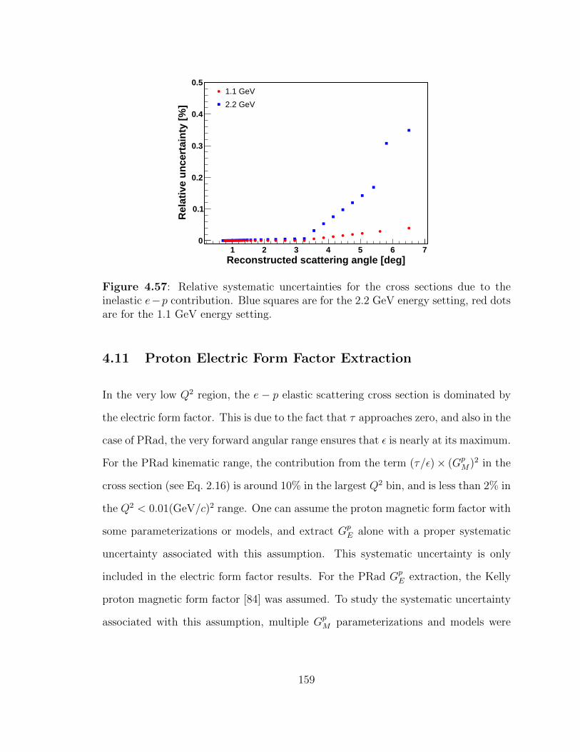
Reconstructed scattering angle [deg]1 2 3 4 5 6 7
Rel
ativ
e u
nce
rtai
nty
[%
]
0
0.1
0.2
0.3
0.4
0.51.1 GeV
2.2 GeV
Figure 4.57: Relative systematic uncertainties for the cross sections due to theinelastic e−p contribution. Blue squares are for the 2.2 GeV energy setting, red dotsare for the 1.1 GeV energy setting.
4.11 Proton Electric Form Factor Extraction
In the very low Q2 region, the e− p elastic scattering cross section is dominated by
the electric form factor. This is due to the fact that τ approaches zero, and also in the
case of PRad, the very forward angular range ensures that ε is nearly at its maximum.
For the PRad kinematic range, the contribution from the term (τ/ε)× (GpM)2 in the
cross section (see Eq. 2.16) is around 10% in the largest Q2 bin, and is less than 2% in
the Q2 < 0.01(GeV/c)2 range. One can assume the proton magnetic form factor with
some parameterizations or models, and extract GpE alone with a proper systematic
uncertainty associated with this assumption. This systematic uncertainty is only
included in the electric form factor results. For the PRad GpE extraction, the Kelly
proton magnetic form factor [84] was assumed. To study the systematic uncertainty
associated with this assumption, multiple GpM parameterizations and models were
159

used [90, 91, 92, 93, 94], including the standard dipole form,
GpM,dipole = µp
1
(1 + Q2
0.71(GeV/c)2)2, (4.32)
where µp is the magnetic moment of a proton. These GpM parameterizations are
shown in the top plot of Fig. 4.58. The difference between these parameterizations is
around 2% in the largest Q2 bin and less than 0.5% in the Q2 < 0.01(GeV/c)2 range.
The relative differences between the extracted GpE using other Gp
M parameterizations
or models, and the GpE extracted using the Kelly Gp
M parameterization are shown
in the bottom plot of Fig. 4.58. The extracted GpE varies by no more than 0.3% at
Q2 = 0.06 (GeV/c)2, which is the largest Q2 accessible to the experiment, and <
0.01% in the Q2 < 0.01 (GeV/c)2 region. The total relative systematic uncertainties
of GpE, including the additional source related to the Gp
M assumption, are shown
in Fig. 4.59. The extracted proton electric form factors GpE from both the 1.1 and
2.2 GeV data sets are shown in Fig. 4.60.
160

] 2 [(GeV/c)2Q
3−10 2−10
Kel
lyM
/GM
G
0.99
0.995
1
1.005
1.01
1.015
1.02
1.025
1.03 Bernauer 2010Higinbotham unbound fit 2019Higinbotham bound fit 2019Standard dipoleArrington 2004Arrington 2007Venkat 2011
] 2 [(GeV/c)2Q
3−10 2−10
) [%
]E
/(G
EG∆
0.3−
0.2−
0.1−
0
0.1
0.2
0.3Bernauer 2010Higinbotham unbound fit 2019Higinbotham bound fit 2019Standard dipoleArrington 2004Arrington 2007Venkat 2011
Figure 4.58: Top plot: Different GpM parameterizations [90, 91, 92, 93, 94],
divided by the Kelly GpM parameterization [84]. Bottom plot: The relative
difference between the extracted GpE using other Gp
M parameterizations or mod-els [90, 91, 92, 93, 94] and the extracted Gp
E using the Kelly GpM parameterization [84].
161

Reconstructed scattering angle [deg]1 2 3 4 5 6 7
Rel
ativ
e u
nce
rtai
nty
[%
]
0
0.1
0.2
0.3
0.4
0.5
0.6
0.7
0.8
0.9
11GeV
2GeV
Figure 4.59: The total relative systematic uncertainties of the proton electric formfactor Gp
E for the 1.1 and 2.2 GeV data sets.
Figure 4.60: The extracted proton electric form factors GpE from both the 1.1 (red)
and 2.2 GeV (blue) data sets. The proton magnetic form factor GpM is assumed to be
the Kelly form factor [84] in the extraction. Statistical uncertainties are shown as theerror bars, systematic uncertainties are shown as the shadow bands at the bottom.
162

Chapter 5
Radius Extraction
The slope of GpE(Q2) as Q2 →0 is directly proportional to r2
p (see Eq. 1.1). A common
practice is to fit GpE(Q2) to a functional form and then obtain rp by extrapolating to
Q2 = 0. However, each functional form handles the higher order effects of GpE(Q2)
differently and may introduce a model-dependent bias in the extrapolated rp result.
Thus, it is critical to choose a robust functional form that is most likely to yield
an unbiased determination of rp given the uncertainties in the data set, and test
the chosen functional form over a broad range of parametizations of GpE(Q2). This
study was discussed in the paper of X. Yan, et al. [12] and will be summarized in
Section 5.1 of this chapter. To determine the systematic uncertainty in rp, a Monte
Carlo technique was used to randomly smear the cross section and GE(Q2) data
points for each known source of systematic uncertainties, which were described in
Section 4.10 and Section 4.11. The rp was extracted from the smeared data and the
process was repeated 100,000 times. The RMS of the rp distribution was recorded
as the systematic uncertainty. The studies related to the systematic uncertainty of
rp will be discussed in Section 5.2 of this chapter. Due to the fact that different
normalization uncertainties might exist between the 1.1 and 2.2 GeV data sets, the
radius result was obtained by introducing two independent normalization constants
n1 and n2 to the 1.1 and 2.2 GeV data sets, respectively, but the Q2-dependence was
kept identical during the fitting. The proton charge radius result will be discussed in
Section 5.3 of this chapter.
163

5.1 Search for Robust Fitters
As described in [12], to search for the robust fitters for the PRad data set, first of all, a
large number of pseudo-data sets were generated based on a number of well-known GpE
parameterizations and models [84, 93, 94, 95, 96, 97, 98] with known input rp values.
The pseudo-data points were sampled based on the PRad Q2 range, binning and
statistical uncertainties. Second, a number of functional forms for GpE (fitters) were
used to fit and extract rp from these pseudo-data sets. These GpE parameterizations
are summarized in the following list, with pi as free parameters:
• Dipole:
GpE(Q2) =
(1 +
Q2
p1
)−2, (5.1)
where rp can be determined as√
12/p1.
• Monopole:
GpE(Q2) =
(1 +
Q2
p1
)−1, (5.2)
where rp can be determined as√
6/p1.
• Gaussian:
GpE(Q2) = e−Q
2/p1 , (5.3)
where rp can be determined as√
6/p1.
• Multi-parameter polynomial expansion of Q2:
GpE(Q2) = 1 +
N∑i=1
piQ2i, (5.4)
where rp can be determined as√−6p1 and the maximum order N is defined by
the user.
164

• Multi-parameter rational function of Q2 (rational (N,M)):
GpE(Q2) =
1 +∑N
i=1 paiQ
2i
1 +∑M
j=1 pbjQ
2j, (5.5)
where rp can be determined as√
6(pb1 − pa1) and the maximum order N and M
are defined by the user.
• Continuous fraction expansion:
GpE(Q2) =
1
1 + p1Q2
1+p2Q
2
1+...
, (5.6)
where rp can be determined as√
6p1.
• Multi-parameter polynomial expansion of z:
GpE(Q2) = 1 +
N∑i=1
pizi, (5.7)
after making a conformal mapping through [13]:
z =
√Tc +Q2 −
√Tc − T0√
Tc +Q2 +√Tc − T0
, (5.8)
where Tc = 4m2π, mπ is the mass of a π0 meson, and T0 is a free parameter
representing the point that is mapping onto z = 0 (T0 = 0 for this study). The
charge radius is given by rp =√−3p1/2Tc.
In addition, it is a common practice to include an additional normalization parameter
(floating parameter) to handle systematic uncertainties associated with the normal-
165

ization of the data points, such that the final functional form of a fitter is
f(Q2) = nGpE(Q2), (5.9)
where n is the floating parameter and GpE(Q2) can be any of the functions listed
above.
Lastly, the mean value and RMS of the extracted rp values were compared to the
input rp. In addition to minimizing the value of the Root-Mean-Square Error (RMSE
=√
bias2 + RMS2), it is also required that a robust fitter must have the mean value of
the extracted rp agree with the input rp within the value of the RMS, for all the input
form factor models used in the test. The results for some of the fitters are shown in
Fig 5.1 to Fig 5.4, which apply to the entire PRad kinematic range (1.1 and 2.2 GeV
data sets together). Single parameter fitters (excluding the floating parameter) such
as the dipole, monopole, Gaussian and the first order polynomial expansion of Q2
and z tend to give biased results with very small uncertainties. Fitters including
more than two parameters (excluding the floating parameter) such as the third order
polynomial expansions of Q2 and z tend to give unnecessarily large uncertainties even
though the results are well consistent with the input rp within their RMS values. The
robust fitters identified from this study include the two-parameter rational function
(rational (1,1)):
f(Q2) = nGE(Q2) = n1 + pa1Q
2
1 + pb1Q2, (5.10)
and the second order polynomial expansion of z (second order z transformation):
f(Q2) = nGE(Q2) = n(1 + p1z + p2z
2). (5.11)
166
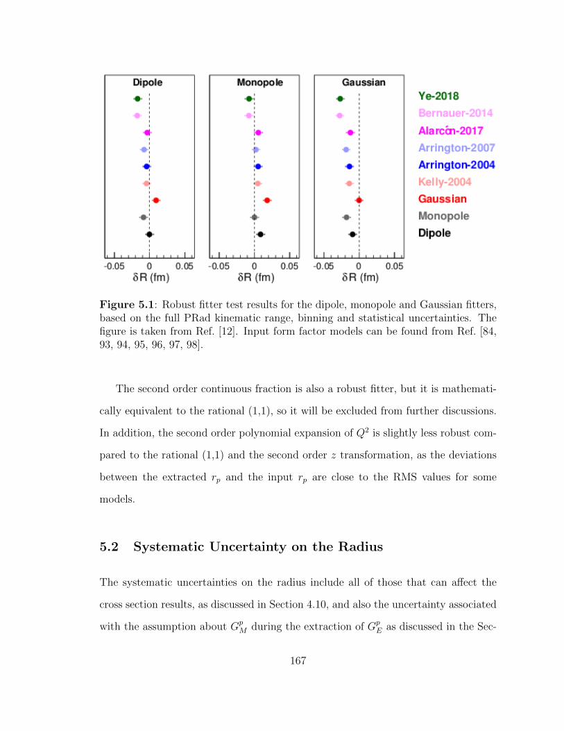
Figure 5.1: Robust fitter test results for the dipole, monopole and Gaussian fitters,based on the full PRad kinematic range, binning and statistical uncertainties. Thefigure is taken from Ref. [12]. Input form factor models can be found from Ref. [84,93, 94, 95, 96, 97, 98].
The second order continuous fraction is also a robust fitter, but it is mathemati-
cally equivalent to the rational (1,1), so it will be excluded from further discussions.
In addition, the second order polynomial expansion of Q2 is slightly less robust com-
pared to the rational (1,1) and the second order z transformation, as the deviations
between the extracted rp and the input rp are close to the RMS values for some
models.
5.2 Systematic Uncertainty on the Radius
The systematic uncertainties on the radius include all of those that can affect the
cross section results, as discussed in Section 4.10, and also the uncertainty associated
with the assumption about GpM during the extraction of Gp
E as discussed in the Sec-
167

Figure 5.2: Robust fitter test results for the multi-parameter polynomial expansionof Q2, based on the full PRad kinematic range, binning and statistical uncertainties.The figure is taken from Ref. [12]. Input form factor models can be found fromRef. [84, 93, 94, 95, 96, 97, 98].
Figure 5.3: Robust fitter test results for the multi-parameter rational function ofQ2, based on the full PRad kinematic range, binning and statistical uncertainties.The figure is taken from Ref. [12]. Input form factor models can be found fromRef. [84, 93, 94, 95, 96, 97, 98].
168

Figure 5.4: Robust fitter test results for the multi-parameter polynomial expansionof z, based on the full PRad kinematic range, binning and statistical uncertainties.The figure is taken from Ref. [12]. Input form factor models can be found fromRef. [84, 93, 94, 95, 96, 97, 98].
tion 4.11. A Monte-Carlo technique was used to evaluate the effect of these system-
atic uncertainties on the radius result. First of all, 100,000 data sets were generated
based on the PRad cross section results. Then the data points were smeared by all
the systematic uncertainty sources at once, and a set of GpE data points was extracted
from each smeared cross section data set. For each systematic uncertainty source, if
it was uncorrelated, then each cross section data point was smeared independently
by a random number generated from a Gaussian distribution, with its width as the
systematic uncertainty of this data point. If the systematic uncertainty source was
correlated, then the correlation between different angular or Q2 data points must be
included in the smearing. Typically, the correlation could be described by low order
polynomials or splines. Then the data points would be multiplied or divided by these
correlation functions. For the mixed uncertainties (partially correlated and partially
uncorrelated), such as those related to event selection cuts, the cross section tables
were generated by randomly choosing the cuts within a given range (± 50% of the
169

nominal kinematic cut for the 2.2 GeV e − p in the PbWO4 region for instance).
For the uncertainty associated with the GpM assumption, a Gp
M model was randomly
selected from Ref. [84, 90, 91, 92, 93, 94], and also the standard dipole model (see
Eq. 4.32), when extracting GpE from the cross section data points.
Second, the extracted GpE data sets were fitted separately and a rp value was
extracted from each of these data sets. Only the statistical uncertainties were used
during these extractions. Lastly, the RMS of these extracted rp values was assigned
as the systematic uncertainty. The distributions for these extracted rp using the
rational (1,1) and the second order z transformation are shown in Fig. 5.5. The
contributions from individual systematic uncertainties are listed in Table 5.1, for the
rational (1,1) fitter. In this case, the data points were smeared by the individual
systematic uncertainty source only, while effects from other sources were turned off.
The table also includes the systematic uncertainties for the normalization parameters
n1 and n2 for the 1.1 and 2.2 GeV data sets respectively. The systematic uncertainties
obtained with the second order z transformation are in general very similar to those
from the rational (1,1), but slightly larger.
5.3 Proton Charge Radius Result
The GpE(Q2) extracted from the 1.1 GeV and 2.2 GeV data sets were fitted simul-
taneously using the rational (1,1) function. Independent normalization parameters
n1 and n2 were assigned to the 1.1 and 2.2 GeV data sets, respectively, to allow
for differences in the normalization uncertainties, but the Q2-dependence was identi-
cal. The normalization parameters and rp obtained from the fit to the rational (1,1)
function are [99]:
170

[fm]pr0.74 0.76 0.78 0.8 0.82 0.84 0.86 0.88 0.9 0.92
cou
nts
0
1
2
3
4
5
6
7
310×
RMS = 0.0115 fm
a
[fm]pr0.74 0.76 0.78 0.8 0.82 0.84 0.86 0.88 0.9 0.92
cou
nts
0
1
2
3
4
5
6
310×
RMS = 0.0135 fm
b
Figure 5.5: Distributions of rp extracted using (a) the rational (1,1) and (b) thesecond order z transformation; from data sets that were smeared by all the PRadsystematic uncertainties. The RMS of the distribution in (a) is 0.0115 fm and thatfor (b) is 0.0135 fm.
171

Item rp uncertainty [fm] n1 uncertainty n2 uncertaintyEvent selection 0.0070 0.0002 0.0006
Radiative correction 0.0069 0.0010 0.0011Detector efficiency 0.0042 0.0000 0.0001Beam background 0.0039 0.0017 0.0003HyCal response 0.0029 0.0000 0.0000
Acceptance 0.0026 0.0001 0.0001Beam energy 0.0022 0.0001 0.0002Inelastic ep 0.0009 0.0000 0.0000
GpM parameterization 0.0006 0.0000 0.0000
Total 0.0115 0.0020 0.0013
Table 5.1: The systematic uncertainty table for rp and the normalization parameters.Items are arranged in decreasing order of the effect on rp. The parameters n1 and n2
are the normalization parameters for the 1.1 GeV and 2.2 GeV data sets, respectively.Uncertainties are estimated using the rational (1,1) function.
rp = (0.831± 0.007stat. ± 0.012syst.) fm,
n1 = 1.0002± 0.0002stat. ± 0.0020syst., (5.12)
n2 = 0.9983± 0.0002stat. ± 0.0013syst..
Only the statistical uncertainties were used when evaluating the central values.
The rational (1,1) fit and the GpE data points from the experiment are shown in
Fig. 5.6, compared to two recent GpE models [96, 97]. The 68% point-wise confidence
level band for the total uncertainties of the result is shown in Fig. 5.7, compared to
those from the same GpE models [96, 97]. The total uncertainties were taken as the
quadratic sum of the total systematic uncertainties and the statistical uncertainties.
The rational (1,1) function describes the data reasonably well, with a reduced
χ2 of 1.3 when considering only the statistical uncertainties. The quality of the fit
is shown in Fig. 5.8, where (a) shows the residuals (differences between data points
172
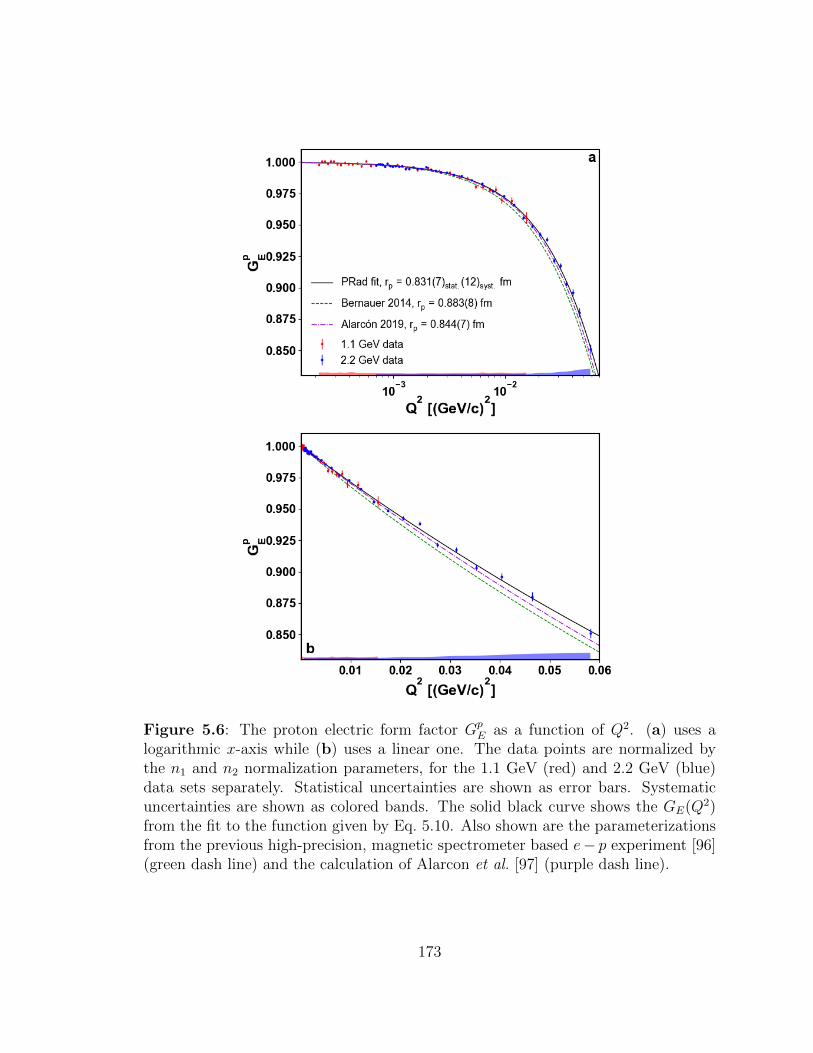
Figure 5.6: The proton electric form factor GpE as a function of Q2. (a) uses a
logarithmic x-axis while (b) uses a linear one. The data points are normalized bythe n1 and n2 normalization parameters, for the 1.1 GeV (red) and 2.2 GeV (blue)data sets separately. Statistical uncertainties are shown as error bars. Systematicuncertainties are shown as colored bands. The solid black curve shows the GE(Q2)from the fit to the function given by Eq. 5.10. Also shown are the parameterizationsfrom the previous high-precision, magnetic spectrometer based e− p experiment [96](green dash line) and the calculation of Alarcon et al. [97] (purple dash line).
173

and the fit) of the fit, and (b) shows the pull distribution (residuals weighted by
the statistical uncertainties of the data points). The largest deviation is about 2.5
standard deviations. For the pull distributions, if the uncertainties describe the
fluctuation in the data points very well, one would expect that about 68% of the
data points fall inside ±1. This number is about 67% for the 1.1 GeV data set and
about 58% for the 2.2 GeV data set.
The results obtained with the second order z transformation are very similar to
those from the rational (1,1): n1 = 1.0002 ± 0.0002stat. ± 0.0021syst., n2 = 0.9983 ±
0.0002stat.± 0.0013syst., and rp = (0.830± 0.008stat.± 0.013syst.) fm. Fig 5.9 shows the
results obtained from the rational (1,1) and the second order z transformation, and
also results obtained from other slightly less robust fitters. Based on our robustness
tests [12], lower order functional forms such as the monopole, dipole, and the first
order expansion of Q2 (not shown here) tend to give smaller statistical uncertainties,
but have larger uncertainties from the truncation of the Q2 range and the extrap-
olation to Q2 = 0, and also tend to produce larger biases depending on the input
GpE(Q2) parametrization used. On the other hand, higher order functional forms such
as the third order polynomial expansion of Q2 (not shown here) and z transformation
tend to give very large overall uncertainties. The results also confirm that rational
(1,1) and the second order z transformation are the most robust fitting functions,
giving the most consistent results with the least uncertainties for the Q2 range of
the PRad experiment.
The consistency of the radius extraction was further studied by extracting rp from
various sub-sets of the experimental data, such as the data collected with only the 1.1
GeV electron beam, only the 2.2 GeV electron beam, just the PbWO4 modules, and
the Q2 range limited to < 0.016 (GeV/c)2 and > 0.002 (GeV/c)2. All the data sub-
sets were fitted with the rational (1,1) functional form and the rp values obtained are
174
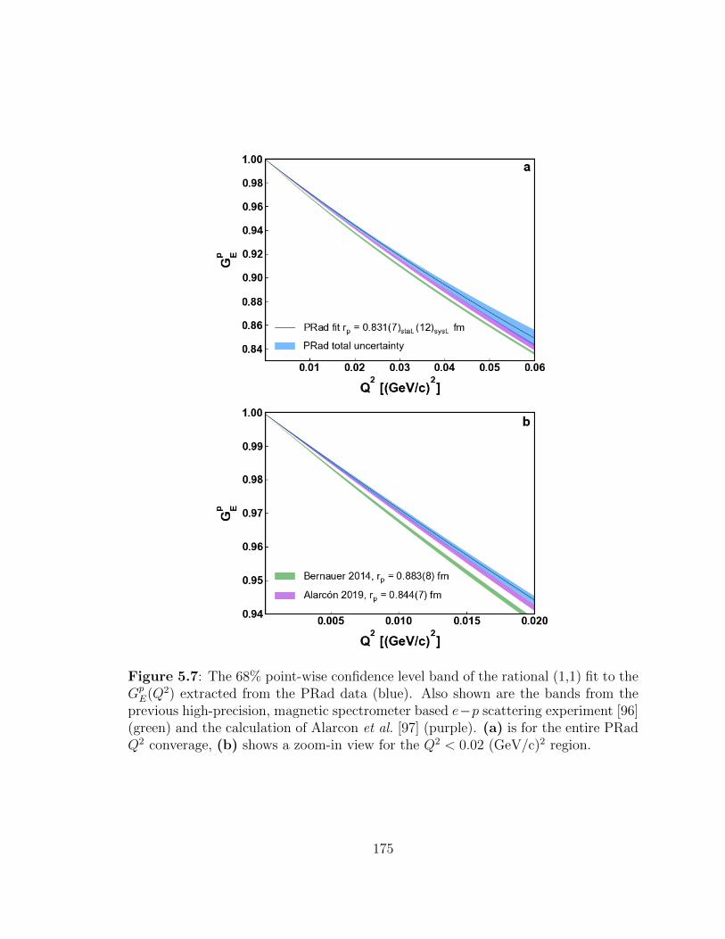
Figure 5.7: The 68% point-wise confidence level band of the rational (1,1) fit to theGpE(Q2) extracted from the PRad data (blue). Also shown are the bands from the
previous high-precision, magnetic spectrometer based e−p scattering experiment [96](green) and the calculation of Alarcon et al. [97] (purple). (a) is for the entire PRadQ2 converage, (b) shows a zoom-in view for the Q2 < 0.02 (GeV/c)2 region.
175

Figure 5.8: (a) shows the residuals between PRad GpE data points and the fit using
the rational (1,1) fitter. Red squares are from the 1.1 GeV data set and blue dotsare from the 2.2 GeV data set. Error bars contain only the statistical uncertainties.(b) shows the pull distributions (residuals weighted by the statistical uncertaintiesof the data points) for the 1.1 GeV (red) and 2.2 GeV (blue) data sets.
176

Figure 5.9: The rp results obtained when using different fitters. Statistical uncer-tainties are shown as error bars, and the total uncertainties (quadratic sum of thetotal systematic and statistical uncertainties) are shown as colored bands. The ratio-nal (1,1) and the second order z transformation are identified as robust fit functionsby Yan et al. [12].
consistent within statistical uncertainties as shown in Fig. 5.10 (a). However, the rp
values extracted from some data sub-sets, such as the ones with restricted Q2 range,
have larger uncertainties because the Q2 coverage is reduced, and the rational (1,1)
is not the most robust functional form for these data sub-sets. This is demonstrated
in Fig. 5.10 (b), where the 1.1 GeV and 2.2 GeV data sets are separately fitted using
the two best functional forms for these particular data sets, as determined from the
robustness study [12].
The statistical fluctuation of the result was studied by separating the entire data
set randomly into 20 subsets (10 for the 1.1 GeV and 10 for the 2.2 GeV settings).
Each subset is then fitted with the same functional form, which is the monopole
fitter for the 1.1 GeV subsets and the rational (1,1) for 2.2 GeV subsets1. The results
1The reason for choosing a lower order fitter for the 1.1 GeV subsets was that the uncertainty byusing the rational (1,1) was too large (over 0.1 fm for each data point).
177

Figure 5.10: (a): the extracted rp values under different conditions, as listed in thefigure. All data points are obtained using the rational (1,1) fitter. Error bars showonly the statistical uncertainties. (b): the monopole and dipole fits for the 1.1 GeVdata points, and the rational (1,1) and the second order z transformation fits for the2.2 GeV data points. Error bars show the statistical uncertainties. Colored bandsshow the total uncertainties.
from the subsets are well consistent statistically with the ones obtained by fitting the
whole data sets, which are almost identical to the weighted averages from the subsets
by their statistical uncertainties, as shown in Fig. 5.3.
Another important study is to extract the rp result using only the integrated
Møller method. As discussed in Section 4.10, a number of dominant systematic un-
certainties are Q2-dependent ones due to the Møller and they affect the result through
the bin-by-bin method, as in this case, the e− p to e− e normalization is performed
separately for each angular bin. On the other hand, for the integrated Møller method,
all systematic uncertainties from the Møller can only affect the normalization of all
data points and cannot introduce any Q2-dependent systematic uncertainty. How-
ever, the integrated Møller method is more sensitive to systematic uncertainties such
as the GEM efficiency, which cannot be determined well enough when the scattering
angles are smaller than 1.3. If one removes all data points below 1.3 for both en-
178
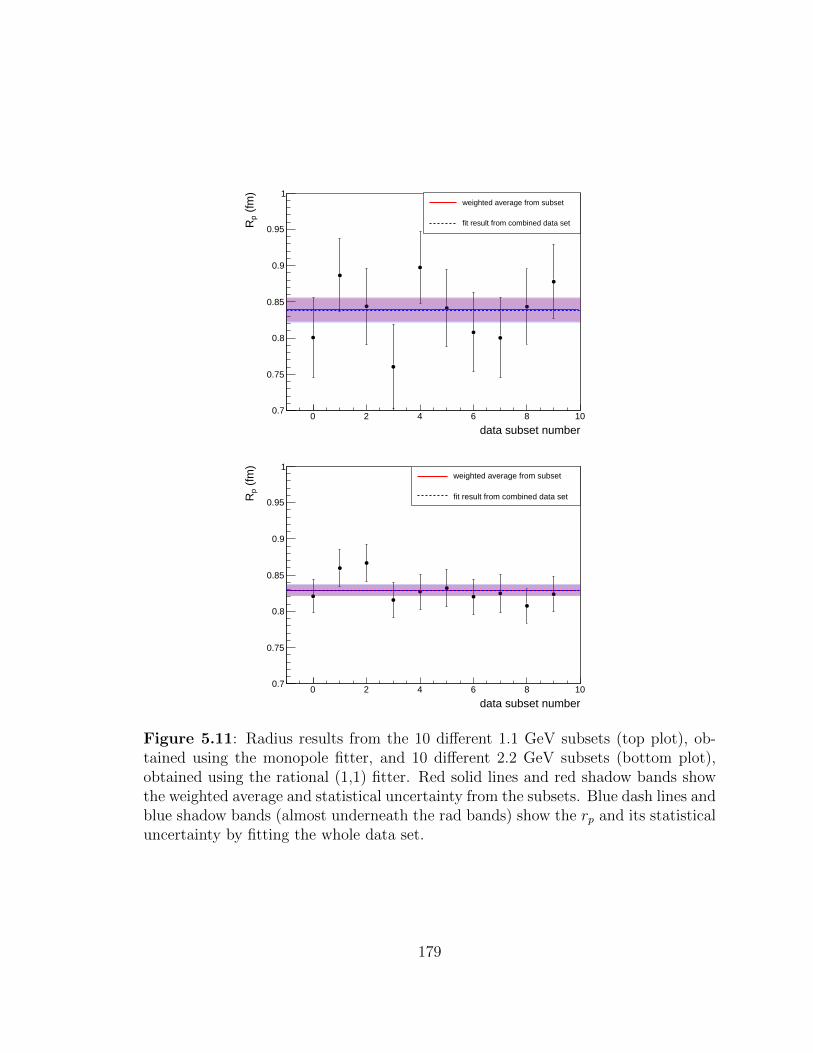
data subset number0 2 4 6 8 10
(fm
)p
R
0.7
0.75
0.8
0.85
0.9
0.95
1weighted average from subset
fit result from combined data set
data subset number0 2 4 6 8 10
(fm
)p
R
0.7
0.75
0.8
0.85
0.9
0.95
1weighted average from subset
fit result from combined data set
Figure 5.11: Radius results from the 10 different 1.1 GeV subsets (top plot), ob-tained using the monopole fitter, and 10 different 2.2 GeV subsets (bottom plot),obtained using the rational (1,1) fitter. Red solid lines and red shadow bands showthe weighted average and statistical uncertainty from the subsets. Blue dash lines andblue shadow bands (almost underneath the rad bands) show the rp and its statisticaluncertainty by fitting the whole data set.
179

ergy settings and apply only the integrated Møller method, the extracted results will
be: n1 = 1.0001± 0.0003stat. ± 0.0018syst., n2 = 0.9984± 0.0004stat. ± 0.0014syst., and
rp = (0.834±0.010stat.±0.008syst.) fm, using the rational (1,1) fitter. They agree with
the results shown in Eq. 5.12 within 1 standard deviation of the statistical uncertain-
ties. In this case, the minimum Q2 will be 6.3× 10⁻⁴ (GeV/c)2 for the 1.1 GeV and
2.4 × 10⁻³ (GeV/c)2 for the 2.2 GeV data sets. In addition, removing data points
below 1.3 also significantly reduces the effect due to the background generated from
the upstream beam halo blocker, which is the dominating background source partic-
ularly in the forward angular region. The consistency of the rp results demonstrates
that the empty target run subtraction was rather effective.
180
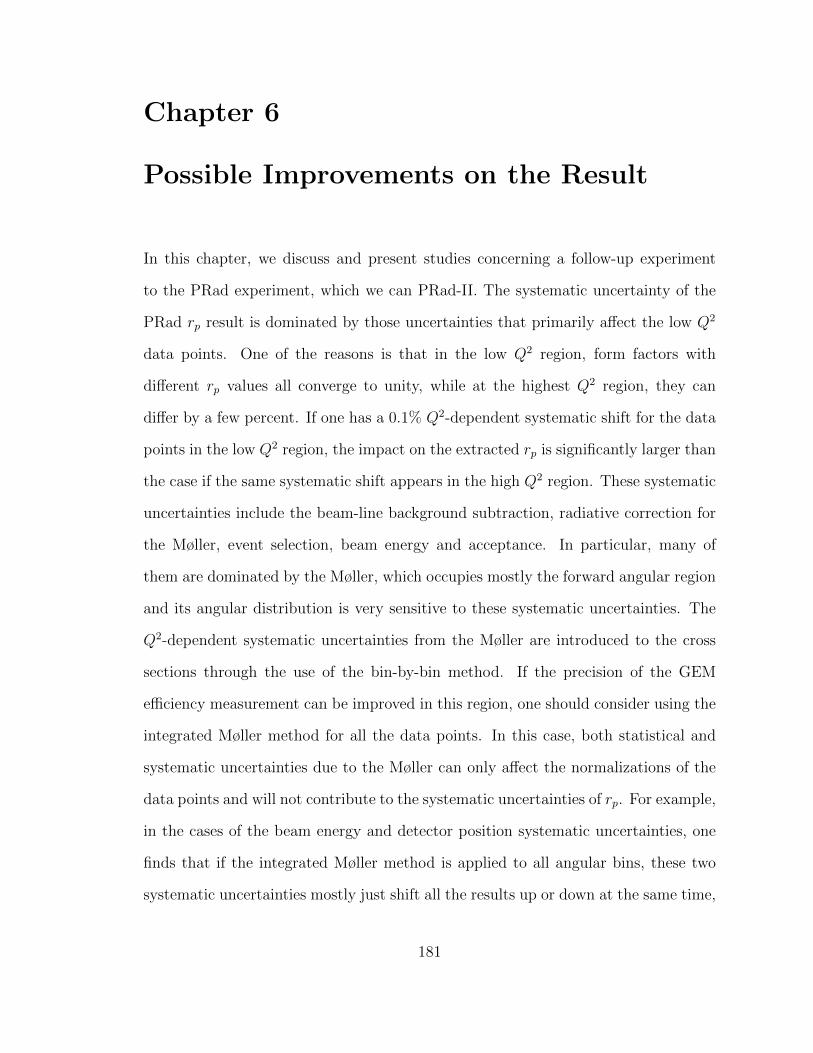
Chapter 6
Possible Improvements on the Result
In this chapter, we discuss and present studies concerning a follow-up experiment
to the PRad experiment, which we can PRad-II. The systematic uncertainty of the
PRad rp result is dominated by those uncertainties that primarily affect the low Q2
data points. One of the reasons is that in the low Q2 region, form factors with
different rp values all converge to unity, while at the highest Q2 region, they can
differ by a few percent. If one has a 0.1% Q2-dependent systematic shift for the data
points in the low Q2 region, the impact on the extracted rp is significantly larger than
the case if the same systematic shift appears in the high Q2 region. These systematic
uncertainties include the beam-line background subtraction, radiative correction for
the Møller, event selection, beam energy and acceptance. In particular, many of
them are dominated by the Møller, which occupies mostly the forward angular region
and its angular distribution is very sensitive to these systematic uncertainties. The
Q2-dependent systematic uncertainties from the Møller are introduced to the cross
sections through the use of the bin-by-bin method. If the precision of the GEM
efficiency measurement can be improved in this region, one should consider using the
integrated Møller method for all the data points. In this case, both statistical and
systematic uncertainties due to the Møller can only affect the normalizations of the
data points and will not contribute to the systematic uncertainties of rp. For example,
in the cases of the beam energy and detector position systematic uncertainties, one
finds that if the integrated Møller method is applied to all angular bins, these two
systematic uncertainties mostly just shift all the results up or down at the same time,
181
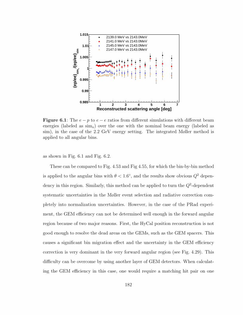
Reconstructed scattering angle [deg]1 2 3 4 5 6 7
sim
/(ep
/ee)
xsi
m(e
p/e
e)
0.985
0.99
0.995
1
1.005
1.01
1.0152139.0 MeV vs 2143.0MeV2141.0 MeV vs 2143.0MeV2145.0 MeV vs 2143.0MeV2147.0 MeV vs 2143.0MeV
Figure 6.1: The e− p to e− e ratios from different simulations with different beamenergies (labeled as simx) over the one with the nominal beam energy (labeled assim), in the case of the 2.2 GeV energy setting. The integrated Møller method isapplied to all angular bins.
as shown in Fig. 6.1 and Fig. 6.2.
These can be compared to Fig. 4.53 and Fig 4.55, for which the bin-by-bin method
is applied to the angular bins with θ < 1.6, and the results show obvious Q2 depen-
dency in this region. Similarly, this method can be applied to turn the Q2-dependent
systematic uncertainties in the Møller event selection and radiative correction com-
pletely into normalization uncertainties. However, in the case of the PRad experi-
ment, the GEM efficiency can not be determined well enough in the forward angular
region because of two major reasons. First, the HyCal position reconstruction is not
good enough to resolve the dead areas on the GEMs, such as the GEM spacers. This
causes a significant bin migration effect and the uncertainty in the GEM efficiency
correction is very dominant in the very forward angular region (see Fig. 4.29). This
difficulty can be overcome by using another layer of GEM detectors. When calculat-
ing the GEM efficiency in this case, one would require a matching hit pair on one
182

Reconstructed scattering angle [deg]0 1 2 3 4 5 6 7
sim
/(ep
/ee)
xsi
m(e
p/e
e)
0.995
0.996
0.997
0.998
0.999
1
1.001
1.002
1.003
1.004
1.005GEM shift -2.0 mmGEM shift -1.0 mmGEM shift 1.0 mmGEM shift 2.0 mm
Figure 6.2: The e − p to e − e ratios from different simulations with shifted GEMpositions (positive shift means shift to down stream, labeled as simx) over the oneobtained from the standard simulation (labeled as sim), in the case of the 2.2 GeVenergy setting. The integrated Møller method is applied to all angular bins.
GEM layer and the HyCal, and then look for whether there is a hit found on the
other GEM layer. The incident angle would be determined by the matching GEM
hit, which will eliminate the bin migration issue due to the HyCal resolution and
non-uniformity in the position reconstruction. The expected systematic uncertainty
in the GEM efficiency correction, due to the GEM dead areas, is shown to be better
than 0.1% (see Fig. 6.3), and the corresponding systematic uncertainty on rp will
be much smaller than that from the PRad. The uncertainty is determined using a
similar approach as discussed in Section 4.6, by comparing the e − p to e − e ratios
obtained using perfect GEM detectors in the simulation and those with more realistic
GEMs including the spacers and other dead areas. This systematic uncertainty can
be further reduced if one assembles the second GEM using a new technique [123],
which requires no spacers in between the GEM foils. Second, the very forward angular
region suffers from the background that is generated from very-small-angle-scattering
183

Reconstructed scattering angle [deg]1 2 3 4 5
sim
/(ep
/ee)
sim
'(e
p/e
e)
0.995
0.996
0.997
0.998
0.999
1
1.001
1.002
1.003
1.004
1.005
Figure 6.3: The expected GEM efficiency correction uncertainty on the cross sectionif a second GEM layer were used.
particles hitting the downstream beam pipe and other surrounding objects (see Sec-
tion 4.5.4). This type of background cannot be rejected by the HyCal alone, but can
be rejected when combining one GEM layer and the HyCal, since these tracks cannot
be projected back to the target region. In addition, other backgrounds for the GEM
efficiency measurement, such as the cosmic events and high energy photons, will be
rejected easily by having a second GEM layer. The collaboration is currently working
on more detailed simulations to study the improvement of the GEM efficiency. We
will also consider using the overlapping region of the PRad GEM data (there was a
4.4 cm × 123 cm overlapping region for PRad GEMs, see Section 3.4) to demonstrate
the improvement, as in this case there were two separated GEM planes in this region.
Another benefit of having two separated GEM detector layers is that, once the
distance in between the two layers is large enough, one can reconstruct the vertex-z
184

New GEM
PRadGEM
HyCal
Vacuum chamber
Figure 6.4: The proposed experimental setup for PRad-II.
for the e − p events with a reasonable resolution in order to reject the background
that is generated very far away from the target center. In particular, it can reject
the background generated from the upstream beam halo blocker, which is about 2 m
upstream from the target and its background is a few times larger than all the other
beam-line backgrounds combined. This can significantly suppress the systematic un-
certainties related to the beam-line background subtraction. The proposed setup will
have the PRad HyCal and GEMs pushed slightly downstream and have the second
GEM layer placed immediately after the vacuum chamber, as shown in Fig. 6.4. With
a 40 cm distance between the two GEM layers, the vertex-z resolution can be better
than 30 cm as shown in Fig. 6.5 for the 2.2 GeV beam setting, which is sufficient to
reject the background generated from the upstream halo blocker. The resolution can
be further improved by using a thiner aluminum vacuum window (0.8 mm instead
of 1.6 mm as for the PRad experiment for example), or by pushing the PRad GEMs
and the HyCal slightly downstream, at a cost of sacrificing slightly the maximum Q2
185

Figure 6.5: The vertex-z resolution for the e−p events as a function of the scatteringangle, reconstructed using two GEMs layers that are separated by 40 cm, for the2.2 GeV beam energy setting. For the red dots, the simulation uses a 1.6 mm thickaluminum vacuum window, which is true in the case of the PRad experiment. Theblack triangles assume a 0.8 mm thick vacuum window. The plot is taken from [124].
coverage.
Other than the possible improvements mentioned above, there is a plan to include
calculations for the next-to-next-leading order Feynman diagrams in the radiative
correction (currently only the next-to-leading order diagrams included), which will
further reduce this systematic uncertainty. The dominant part is the Møller radiative
correction and it can already be reduced by using the integrated Møller method. The
remaining part comes from the e − p elastic scattering, and it should be reasonable
to assume that even higher order contributions should be one order of magnitude
smaller than that from the next-to-next-leading order. The future experiment should
also consider to increase the statistics by a factor or 4 at least so that the statistical
uncertainty of rp can be suppressed to a 0.003 fm level. The increase of statistics
can also help reducing the systematic uncertainties due to the event selection and
HyCal response in the large angular region. For the PRad experiment, the energy
186

spectrum agreement between the data and simulation is significantly worse in the
Pb-glass region. As shown in Fig. 4.47 and Fig. 4.48, the variation on the cross
section is significantly larger if one changes the size of the event selection cuts, com-
pared to the PbWO4 region. This is partially due to the lack of statistics for the
energy calibration of the HyCal. And also for the same reason, one has to combine
multiple modules to extract certain properties, such as their light attenuation and
non-uniformity properties in the energy reconstruction. With more statistics, these
types of studies can be done module by module, and thus improving the agreement
between the data and the simulation. It should be reasonable to assume a factor of
2 reduction for the systematic uncertainties associated with the event selection and
HyCal response in the large angular region. With 4 times more statistics, a second
GEM layer, the planned use of the integrated Møller method for all data points and
the same beam energy settings as for the PRad experiment, the projected statistical
and systematic uncertainty for PRad-II are shown in Table 6.1 (as PRad-II type A),
and compared to those from the PRad experiment. The major improvement comes
from the planned use of the integrated Møller method for all data points. This item
alone can already reduce the total systematic uncertainty by about a factor of 2, as
long as the GEM efficiency is known to better than 0.1% precision. As discussed
earlier in this chapter, this method will turn all the systematic uncertainties from the
Møller into normalization uncertainties, and thus will not introduce any systematic
uncertainties in rp. Such systematic uncertainties include the Møller event selection,
Møller radiative correction, acceptance and beam energy. Further improvements may
come from the rejection of some beam-line background using two GEM planes, fixing
all the dead modules of the HyCal, better modeling for the HyCal response, better
simulation for the target gas profile and so on.
The future experiment can also exploit possible benefits from enlarging the Q2
187
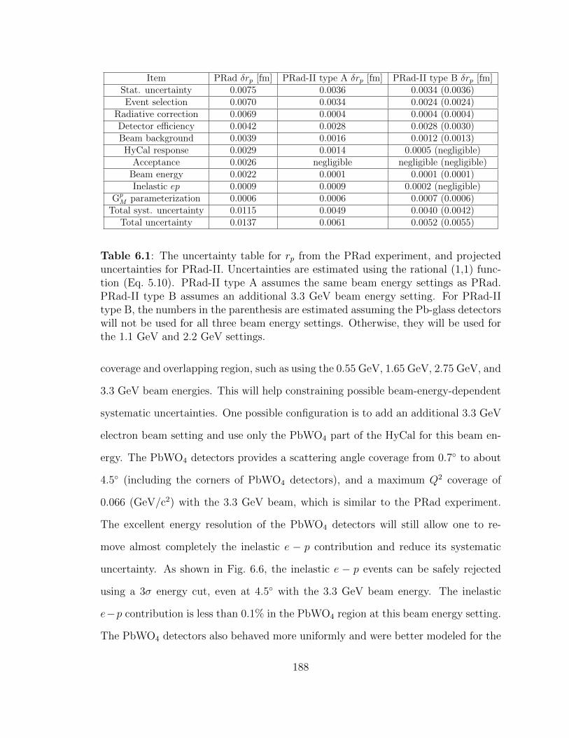
Item PRad δrp [fm] PRad-II type A δrp [fm] PRad-II type B δrp [fm]Stat. uncertainty 0.0075 0.0036 0.0034 (0.0036)Event selection 0.0070 0.0034 0.0024 (0.0024)
Radiative correction 0.0069 0.0004 0.0004 (0.0004)Detector efficiency 0.0042 0.0028 0.0028 (0.0030)Beam background 0.0039 0.0016 0.0012 (0.0013)HyCal response 0.0029 0.0014 0.0005 (negligible)
Acceptance 0.0026 negligible negligible (negligible)Beam energy 0.0022 0.0001 0.0001 (0.0001)Inelastic ep 0.0009 0.0009 0.0002 (negligible)
GpM parameterization 0.0006 0.0006 0.0007 (0.0006)
Total syst. uncertainty 0.0115 0.0049 0.0040 (0.0042)Total uncertainty 0.0137 0.0061 0.0052 (0.0055)
Table 6.1: The uncertainty table for rp from the PRad experiment, and projecteduncertainties for PRad-II. Uncertainties are estimated using the rational (1,1) func-tion (Eq. 5.10). PRad-II type A assumes the same beam energy settings as PRad.PRad-II type B assumes an additional 3.3 GeV beam energy setting. For PRad-IItype B, the numbers in the parenthesis are estimated assuming the Pb-glass detectorswill not be used for all three beam energy settings. Otherwise, they will be used forthe 1.1 GeV and 2.2 GeV settings.
coverage and overlapping region, such as using the 0.55 GeV, 1.65 GeV, 2.75 GeV, and
3.3 GeV beam energies. This will help constraining possible beam-energy-dependent
systematic uncertainties. One possible configuration is to add an additional 3.3 GeV
electron beam setting and use only the PbWO4 part of the HyCal for this beam en-
ergy. The PbWO4 detectors provides a scattering angle coverage from 0.7 to about
4.5 (including the corners of PbWO4 detectors), and a maximum Q2 coverage of
0.066 (GeV/c2) with the 3.3 GeV beam, which is similar to the PRad experiment.
The excellent energy resolution of the PbWO4 detectors will still allow one to re-
move almost completely the inelastic e − p contribution and reduce its systematic
uncertainty. As shown in Fig. 6.6, the inelastic e − p events can be safely rejected
using a 3σ energy cut, even at 4.5 with the 3.3 GeV beam energy. The inelastic
e−p contribution is less than 0.1% in the PbWO4 region at this beam energy setting.
The PbWO4 detectors also behaved more uniformly and were better modeled for the
188

E' [MeV]2000 2200 2400 2600 2800 3000 3200 3400
Co
un
ts
0
500
1000
1500
2000
2500
3000elastic e-pinelastic e-p
[deg]θ0.5 1 1.5 2 2.5 3 3.5 4 4.5
Rat
io
0
0.0005
0.001
Figure 6.6: Left plot: the energy spectrums for the elastic (black histogram) andinelastic (red histogram) e−p with the 3.3 GeV beam energy at around 4.5 scatteringangle. Only the PbWO4 part of the HyCal is used. The blue dash line indicates a3σ kinematic cut. Right plot: the ratio between the inelastic e− p and elastic e− pcounts with 3.3 GeV beam energy as a function of the scattering angle θ, using the3σ kinematic cut.
PRad experiment. Thus the systematic uncertainties associated with HyCal response
and event selection are also expected to be under better control.
A possible PRad-II type B run plan consists of both 1.1 and 2.2 GeV runs with 2
times more statistics compared to the PRad, and an additional 3.3 GeV setting using
only the PbWO4 part of the HyCal. The beam time for the 3.3 GeV setting is assumed
to be roughly 260 hours with a 55 nA beam current (included 52 hours of beam time
for the empty target runs). This plan can produce a similar statistical uncertainty
for rp as the PRad-II type A. The Q2 coverage for each beam energy setting and the
projected relative statistical uncertainties on the cross section are shown in Fig. 6.7.
An advantage of this run plan is that, the e−p elastic scattering cross section will be
measured at least twice for most part of the total Q2 coverage, which is very useful
for cross-checking the beam-energy-dependent systematic uncertainties.
Since the beam energy setting is different, it is also important to study the robust-
ness of the rational (1,1) fitter for this configuration. The results, obtained following
189
]2 [(GeV/c)2Q4−10 3−10 2−10 1−10
Cro
ss s
ecti
on
sta
t. u
nce
rtai
nty
[%
]
1.5−
1−
0.5−
0
0.5
1
1.51.1 GeV2.2 GeV3.3 GeV
Figure 6.7: The Q2 coverage and the relative statistical uncertainties for the crosssections for each beam energy setting in the PRad-II type B run plan.
the same approach in Ref. [12], are shown in Fig. 6.81. The study indicates that the
rational (1,1) fitter is still a robust fitter for this configuration. Assuming a second
GEM layer will be available, the projected statistical and systematic uncertainties for
the PRad-II type B are shown in Table 6.1, and compared to those from the PRad
experiment. The improvement is also dominated by the use of the integrated Møller
method for all data points. For both types of the PRad-II experiments, the expected
total uncertainties on rp are over two times smaller than that from the PRad exper-
iment. The projected total uncertainties are shown in Fig. 6.9, along with the PRad
result and other recent rp measurements.
1The form factor model from Ref. [98] is removed from the test as the rp parameter was fixed tothe CODATA-2014 value during fitting. This approach is different from the fitting proceduresused for other form factor models used in the robustness test.
190

[fm]pr∆0.015− 0.01− 0.005− 0 0.005 0.01 0.015 0.02
Bernauer-2010
Bernauer-2014
Alarcon
Arrington-2007
Arrington-2004
Venkat
Kelly-2004
Gaussian
monopole
dipole
Figure 6.8: Robust fitter test results for the rational (1,1) fitter, based on thePRad-II type B kinematic range, binning and statistical uncertainties, as shown inFig. 6.7. Input form factor models can be found from [84, 90, 93, 94, 95, 96, 97, 92].
[fm]p
Proton charge radius r0.78 0.8 0.82 0.84 0.86 0.88 0.9 0.92
CODATA-2014
CODATA-2014 (ep scatt.)
CODATA-2014 (H spect.)
H spect.)µAntognini 2013 (
H spect.)µPohl 2010 (
Beyer 2017 (H spect.)
Fleurbaey 2018 (H spect.)
Bernauer 2010 (ep scatt.)
CODATA-2018
Mihovilovic 2019(ep scatt.)
Bezginov 2019 (H spect.)
PRad exp. (ep scatt.)PRad-II (type-A) proj.PRad-II (type-B) proj.
Figure 6.9: Projected total uncertainties on rp for PRad-II type A and type B runplans are shown along with the PRad rp result and other recent rp measurements.
191
Chapter 7
Conclusion
In conclusion, this dissertation presents the analysis and results for the PRad ex-
periment, which measured the proton electric form factor GpE in the Q2 region
Q2 = 2.1 × 10⁻⁴ − 0.06 (GeV/c)2. The PRad rp result, obtained by fitting GpE
using the rational (1,1) function, is shown in Figure 7.1, with statistical and sys-
tematic uncertainties summed in quadrature. The result is also compared with a
number of previous rp measurements. It shows a significant discrepancy compared
to results obtained from previous e− p elastic scattering experiments. For instance,
it is about 3-standard deviations smaller than the high-precision electron scattering
measurement at MAMI [5], which was a spectrometer based experiment and the Q2
was limited to higher values (> 0.0038 (GeV/c)2), and it is about 2.7-standard devia-
tions smaller than the CODATA-2014 recommended value for rp based on the results
from previous e− p scattering experiments. However, the result of this experiment is
in agreement with the muonic hydrogen spectroscopic measurements [1, 6], and also
two recent ordinary hydrogen spectroscopic results including the 2S-4P transition
frequency measurement [18] and the 2S-2P Lamb shift measurement [20]. This result
is also consistent with the most recent announced rp value from CODATA-2018 [100].
The result of this experiment does not support any fundamental difference between
the e− p and µ− p interactions.
The comparison between the PRad GpE and a number of previous measured Gp
E
data sets [15, 36, 37] are shown in Fig. 7.2. The top plot shows the full PRad Q2
range and the bottom plot shows only the Q2 < 0.02 (GeV/c)2 range. The GpE data
set for the Mainz 2010 experiment [5, 96] is obtained from Ref. [15]. Generally speak-
192

[fm]pProton charge radius r0.78 0.8 0.82 0.84 0.86 0.88 0.9 0.92
CODATA-2014
CODATA-2014 (ep scatt.)
CODATA-2014 (H spect.)
H spect.)µAntognini 2013 (
H spect.)µPohl 2010 (
Beyer 2017 (H spect.)
Fleurbaey 2018 (H spect.)
Bernauer 2010 (ep scatt.)
CODATA-2018
Mihovilovic 2019(ep scatt.)
Bezginov 2019 (H spect.)
This work (ep scatt.)
σ2.7
Figure 7.1: The rp extracted from the PRad data, shown along with the othermeasurements of rp since 2010 and the CODATA recommended values. The PRadresult is 2.7-σ smaller than the CODATA recommended value for e − p scatteringexperiments [7]. Other results can be found from [1, 5, 6, 18, 19, 20, 22, 100]
ing, the PRad GpE data points are consistent with the previous measurements in the
Q2 < 0.02 (GeV/c)2 range, while the PRad points are consistently larger in the higher
Q2 range. To understand this difference, one may consider various systematic uncer-
tainties of these experiments. The PRad experiment is less sensitive to systematic
uncertainties associated with the integrated luminosity of the measurement, as the
Møller scattering was measured simultaneously and data points with difference Q2
were collected at the same time. However, it is more sensitive to inelastic e− p con-
tribution due to a worse energy resolution compared to magnetic spectrometers, and
also to the detector response of the Pb-glass shower detectors of the HyCal. System-
atic uncertainties due to these two sources can be reduced significantly for PRad-II
as discussed in Ch. 6. The difference may also arise from radiative corrections, which
are quite different for the PRad experiment and other magnetic-spectrometer-based
experiments. Lastly, the difference may be also related to the proton magnetic form
193

factor contribution in the cross section. Important inputs can be obtained in the
future from high precision GpM measurements at very low Q2. Such measurements
may be provided by experiments such as (but not limited to) Ref. [25, 53].
The comparison between the rp result obtained from this experiment, and other
rp results from previous e− p elastic scattering experiments and analyses are shown
in Fig. 7.31. Compared to the previous measurements, the PRad experiment used a
spectrometer-free approach and is the first e−p elastic scattering experiment to cover
two orders of magnitude of low Q2 region in one detector setting. This means that for
each beam energy setting, data points at different Q2 were recorded simultaneously,
with all the detectors fixed in location for the entire data taking process. This elimi-
nates the need for having vast multitude of normalization parameters, which may in-
troduce additional systematic uncertainties to the result. The lowest Q2 measured by
this experiment, 2.1×10⁻⁴(GeV/c)2, is currently the lowest measured value for all e−p
elastic scattering experiments. This reduces the uncertainties due to extrapolation
in the rp extraction. Further measurements for rp are certainly needed particularly
from lepton-proton elastic scattering experiments. A number of e−p and µ−p elastic
scattering experiments are currently under preparation [21, 23, 24, 25, 26, 27, 53],
which will certainly provide useful inputs for the puzzle. The initial state radiation
technique has been proven to be viable by the ISR experiment at MAMI [22], and a
new experiment is planned using the same technique, but with a point-like jet target
and an improved spectrometer entrance flange to further reduce the systematic un-
certainties [21]. An important result is expected in the next few years from the MUSE
collaboration [23], which will use e+, e−, µ+ and µ− beams to perform lepton-proton
elastic scattering measurements, and has a sufficiently large Q2 coverage (0.002 to
0.07 (GeV/c)2). The expected precision on rp is about 0.01 fm for each of the incident
1Thanks to Douglas Higinbotham for providing all the references for the plot.
194
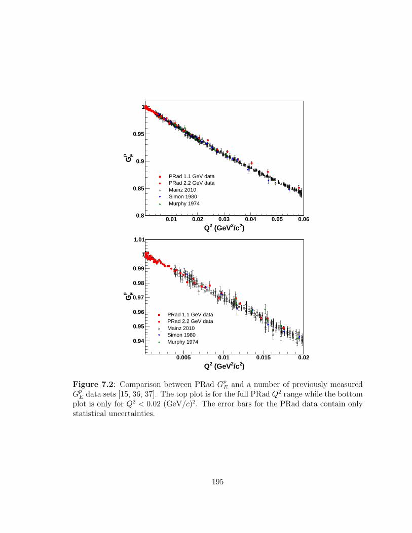
)2/c2 (GeV2Q0.01 0.02 0.03 0.04 0.05 0.06
p EG
0.8
0.85
0.9
0.95
1
PRad 1.1 GeV dataPRad 2.2 GeV dataMainz 2010Simon 1980Murphy 1974
)2/c2 (GeV2Q0.005 0.01 0.015 0.02
p EG
0.94
0.95
0.96
0.97
0.98
0.99
1
1.01
PRad 1.1 GeV dataPRad 2.2 GeV dataMainz 2010Simon 1980Murphy 1974
Figure 7.2: Comparison between PRad GpE and a number of previously measured
GpE data sets [15, 36, 37]. The top plot is for the full PRad Q2 range while the bottom
plot is only for Q2 < 0.02 (GeV/c)2. The error bars for the PRad data contain onlystatistical uncertainties.
195

leptons. This experiment can directly test the lepton universality and will be very
important for fully resolving the proton charge radius puzzle. In addition, the PRad
collaboration has a plan to perform a follow-up experiment to the PRad experiment.
As discussed in Chapter 6, this new experiment will include a second GEM plane to
improve the tracking capacity and the precision of the GEM efficiency measurements,
which allows the application of the integrated Møller method to all angular bins. It
is quite possible that the new experiment can reduce the total uncertainty of rp by a
factor of 2 to 3, compared to the PRad result.
196

Figure 7.3: The rp extracted from the PRad data (black squares), shown along withthe other measurements or analyses of rp from e − p elastic scattering experiments(blue dots). Data points are obtained from references (bottom to top) [30, 101, 102,37, 48, 95, 103, 104, 36, 105, 106, 107, 108, 109, 110, 111, 5, 112, 113, 114, 38, 115,116, 117, 118, 119, 120, 13, 15, 16, 121, 97, 122, 22]
197

Appendix A
Cross Section and Form Factor Data
The fitting function (rational (1,1)) used to obtain the PRad final rp result is,
f(Q2) = nGpE(Q2) = n
1 + pa1Q2
1 + pb1Q2, (A.1)
where n is 1.0002 for the 1.1 GeV data set and 0.9983 for the 2.2 GeV data, pa1 is
-0.07146 and pb1 is 2.88141, both in (GeV/c)−2. Please see Chapter 5 for more details
Table A.1 and Table A.2 contain the cross sections and the f(Q2), that is, they include
the floating parameters n. Our best estimates for the floating parameter n for the
two beam energy settings are listed above. Table A.3 and Table A.4 contain the
proton electric form factor GpE(Q2) without the floating parameter n, i.e. f(Q2)/n.
The bin width for each θ angle bin is shown as “θbw” in Table A.1 and Table A.2.
The polar angle coverage of a polar angle bin goes from θ − 0.5θbw to θ + 0.5θbw.
198

E` θ θbw Q2 σ δσstat. δσsyst. f(Q2) δf(Q2)stat. δf(Q2)syst.
[MeV] [] [] [GeV/c]2 [mb/sr] [mb/sr] [mb/sr] [1] [1] [1]1101 0.7625 0.025 0.000215 2173.30000 4.27660 11.14500 0.99801 0.00098 0.002531101 0.7875 0.025 0.000229 1920.60000 3.95980 9.79210 1.00070 0.00103 0.002521101 0.8125 0.025 0.000244 1694.70000 3.71820 8.38080 1.00060 0.00110 0.002441101 0.8375 0.025 0.000259 1496.80000 3.51490 7.89930 0.99916 0.00117 0.002611101 0.8625 0.025 0.000275 1335.40000 3.33650 6.01830 1.00090 0.00125 0.002221101 0.8875 0.025 0.000291 1190.50000 3.12730 5.51420 1.00060 0.00132 0.002291101 0.9200 0.040 0.000312 1026.60000 2.28790 4.92340 0.99847 0.00111 0.002361101 0.9575 0.035 0.000338 874.24000 2.17710 4.57160 0.99805 0.00124 0.002581101 0.9945 0.039 0.000365 753.64000 1.83400 3.24370 0.99964 0.00122 0.002111101 1.0355 0.043 0.000396 639.98000 1.52630 3.43360 0.99868 0.00119 0.002651101 1.0810 0.048 0.000431 538.60000 1.26520 2.97920 0.99842 0.00117 0.002741101 1.1310 0.052 0.000472 450.10000 1.03500 2.01120 0.99908 0.00115 0.002201101 1.1840 0.054 0.000517 373.16000 0.83371 1.52830 0.99692 0.00111 0.002011101 1.2405 0.059 0.000568 312.19000 0.65870 1.29390 1.00090 0.00106 0.002041101 1.3040 0.068 0.000628 253.75000 0.51715 1.02260 0.99708 0.00102 0.001981101 1.3775 0.079 0.000700 204.03000 0.41431 0.82302 0.99765 0.00101 0.001981101 1.4655 0.097 0.000793 159.52000 0.32207 0.61447 0.99839 0.00101 0.001891101 1.5740 0.120 0.000914 119.67000 0.24211 0.43621 0.99746 0.00101 0.001791101 1.7105 0.153 0.001080 85.90400 0.17184 0.34341 0.99791 0.00100 0.001971101 1.8935 0.213 0.001323 57.04200 0.10879 0.19283 0.99631 0.00095 0.001661101 2.1065 0.213 0.001637 37.08100 0.07857 0.13113 0.99396 0.00106 0.001751101 2.3525 0.279 0.002041 23.93300 0.05027 0.09441 0.99566 0.00105 0.001961101 2.6420 0.300 0.002574 14.97400 0.03506 0.05211 0.99294 0.00117 0.001741101 2.9420 0.300 0.003190 9.72850 0.02670 0.03721 0.99203 0.00137 0.001921101 3.2420 0.300 0.003873 6.55510 0.02000 0.02711 0.98838 0.00152 0.002051101 3.5420 0.300 0.004621 4.59280 0.01651 0.01826 0.98702 0.00179 0.001961101 3.8420 0.300 0.005434 3.27990 0.01337 0.01262 0.98078 0.00202 0.001881101 4.1420 0.300 0.006313 2.42860 0.01090 0.01275 0.98034 0.00223 0.002611101 4.4420 0.300 0.007257 1.82920 0.00887 0.00650 0.97789 0.00241 0.001751101 4.7420 0.300 0.008265 1.41160 0.00735 0.00638 0.97840 0.00259 0.002251101 5.0460 0.308 0.009353 1.08360 0.00619 0.00540 0.96986 0.00283 0.002431101 5.6000 0.800 0.011506 0.71577 0.00377 0.00273 0.96955 0.00262 0.001881101 6.5000 1.000 0.015468 0.38535 0.00374 0.00197 0.95586 0.00480 0.00251
Table A.1: Cross section table for the 1.1 GeV data set.
199
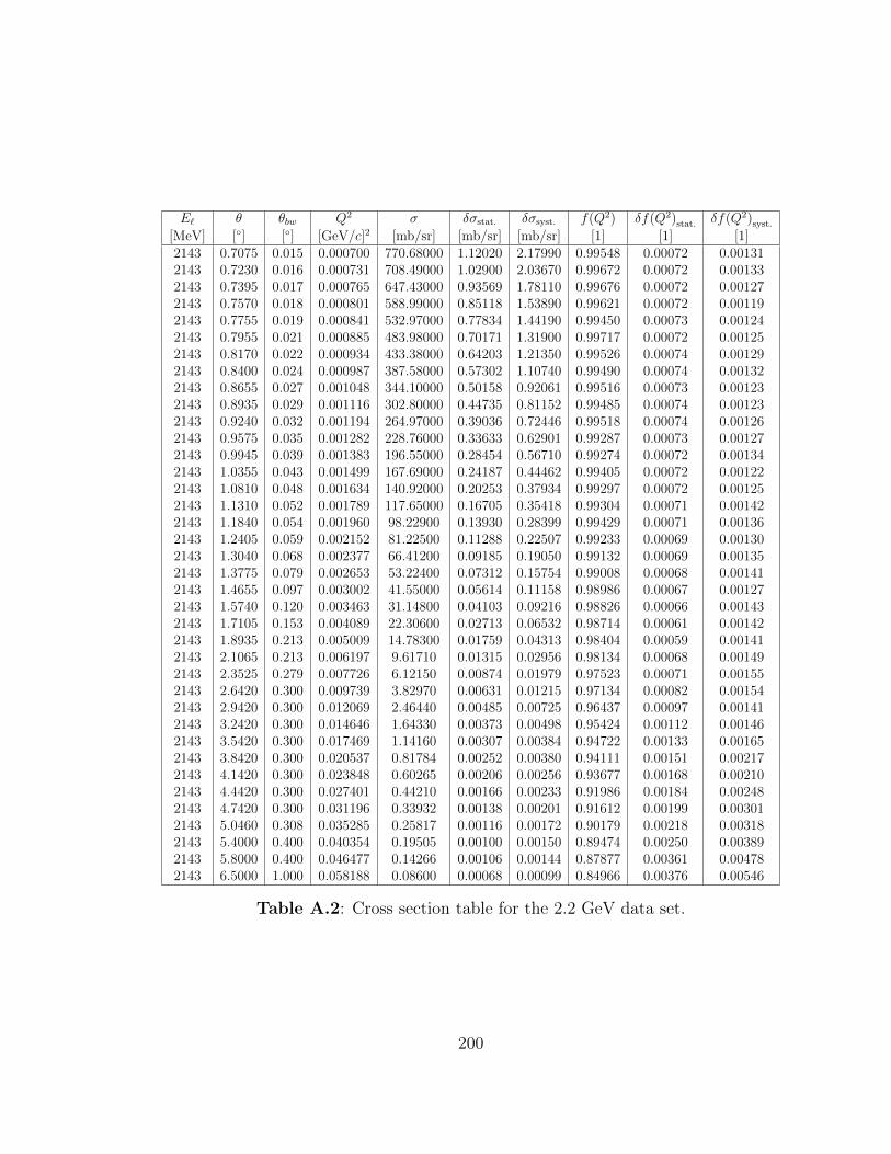
E` θ θbw Q2 σ δσstat. δσsyst. f(Q2) δf(Q2)stat. δf(Q2)syst.
[MeV] [] [] [GeV/c]2 [mb/sr] [mb/sr] [mb/sr] [1] [1] [1]2143 0.7075 0.015 0.000700 770.68000 1.12020 2.17990 0.99548 0.00072 0.001312143 0.7230 0.016 0.000731 708.49000 1.02900 2.03670 0.99672 0.00072 0.001332143 0.7395 0.017 0.000765 647.43000 0.93569 1.78110 0.99676 0.00072 0.001272143 0.7570 0.018 0.000801 588.99000 0.85118 1.53890 0.99621 0.00072 0.001192143 0.7755 0.019 0.000841 532.97000 0.77834 1.44190 0.99450 0.00073 0.001242143 0.7955 0.021 0.000885 483.98000 0.70171 1.31900 0.99717 0.00072 0.001252143 0.8170 0.022 0.000934 433.38000 0.64203 1.21350 0.99526 0.00074 0.001292143 0.8400 0.024 0.000987 387.58000 0.57302 1.10740 0.99490 0.00074 0.001322143 0.8655 0.027 0.001048 344.10000 0.50158 0.92061 0.99516 0.00073 0.001232143 0.8935 0.029 0.001116 302.80000 0.44735 0.81152 0.99485 0.00074 0.001232143 0.9240 0.032 0.001194 264.97000 0.39036 0.72446 0.99518 0.00074 0.001262143 0.9575 0.035 0.001282 228.76000 0.33633 0.62901 0.99287 0.00073 0.001272143 0.9945 0.039 0.001383 196.55000 0.28454 0.56710 0.99274 0.00072 0.001342143 1.0355 0.043 0.001499 167.69000 0.24187 0.44462 0.99405 0.00072 0.001222143 1.0810 0.048 0.001634 140.92000 0.20253 0.37934 0.99297 0.00072 0.001252143 1.1310 0.052 0.001789 117.65000 0.16705 0.35418 0.99304 0.00071 0.001422143 1.1840 0.054 0.001960 98.22900 0.13930 0.28399 0.99429 0.00071 0.001362143 1.2405 0.059 0.002152 81.22500 0.11288 0.22507 0.99233 0.00069 0.001302143 1.3040 0.068 0.002377 66.41200 0.09185 0.19050 0.99132 0.00069 0.001352143 1.3775 0.079 0.002653 53.22400 0.07312 0.15754 0.99008 0.00068 0.001412143 1.4655 0.097 0.003002 41.55000 0.05614 0.11158 0.98986 0.00067 0.001272143 1.5740 0.120 0.003463 31.14800 0.04103 0.09216 0.98826 0.00066 0.001432143 1.7105 0.153 0.004089 22.30600 0.02713 0.06532 0.98714 0.00061 0.001422143 1.8935 0.213 0.005009 14.78300 0.01759 0.04313 0.98404 0.00059 0.001412143 2.1065 0.213 0.006197 9.61710 0.01315 0.02956 0.98134 0.00068 0.001492143 2.3525 0.279 0.007726 6.12150 0.00874 0.01979 0.97523 0.00071 0.001552143 2.6420 0.300 0.009739 3.82970 0.00631 0.01215 0.97134 0.00082 0.001542143 2.9420 0.300 0.012069 2.46440 0.00485 0.00725 0.96437 0.00097 0.001412143 3.2420 0.300 0.014646 1.64330 0.00373 0.00498 0.95424 0.00112 0.001462143 3.5420 0.300 0.017469 1.14160 0.00307 0.00384 0.94722 0.00133 0.001652143 3.8420 0.300 0.020537 0.81784 0.00252 0.00380 0.94111 0.00151 0.002172143 4.1420 0.300 0.023848 0.60265 0.00206 0.00256 0.93677 0.00168 0.002102143 4.4420 0.300 0.027401 0.44210 0.00166 0.00233 0.91986 0.00184 0.002482143 4.7420 0.300 0.031196 0.33932 0.00138 0.00201 0.91612 0.00199 0.003012143 5.0460 0.308 0.035285 0.25817 0.00116 0.00172 0.90179 0.00218 0.003182143 5.4000 0.400 0.040354 0.19505 0.00100 0.00150 0.89474 0.00250 0.003892143 5.8000 0.400 0.046477 0.14266 0.00106 0.00144 0.87877 0.00361 0.004782143 6.5000 1.000 0.058188 0.08600 0.00068 0.00099 0.84966 0.00376 0.00546
Table A.2: Cross section table for the 2.2 GeV data set.
200

E` θ Q2 GpE(Q2) δGp
E(Q2)stat. δGpE(Q2)syst.
[MeV] [] [GeV/c]2 [1] [1] [1]1101 0.7625 0.000215 0.99779 0.00098 0.002531101 0.7875 0.000229 1.00050 0.00103 0.002521101 0.8125 0.000244 1.00040 0.00110 0.002441101 0.8375 0.000259 0.99895 0.00117 0.002601101 0.8625 0.000275 1.00070 0.00125 0.002221101 0.8875 0.000291 1.00040 0.00131 0.002281101 0.9200 0.000312 0.99825 0.00111 0.002361101 0.9575 0.000338 0.99783 0.00124 0.002581101 0.9945 0.000365 0.99942 0.00122 0.002111101 1.0355 0.000396 0.99846 0.00119 0.002651101 1.0810 0.000431 0.99821 0.00117 0.002731101 1.1310 0.000472 0.99886 0.00115 0.002201101 1.1840 0.000517 0.99670 0.00111 0.002011101 1.2405 0.000568 1.00070 0.00106 0.002041101 1.3040 0.000628 0.99686 0.00102 0.001981101 1.3775 0.000700 0.99743 0.00101 0.001981101 1.4655 0.000793 0.99817 0.00101 0.001891101 1.5740 0.000914 0.99724 0.00101 0.001791101 1.7105 0.001080 0.99769 0.00100 0.001971101 1.8935 0.001323 0.99609 0.00095 0.001661101 2.1065 0.001637 0.99374 0.00106 0.001751101 2.3525 0.002041 0.99544 0.00105 0.001961101 2.6420 0.002574 0.99272 0.00117 0.001741101 2.9420 0.003190 0.99181 0.00137 0.001921101 3.2420 0.003873 0.98816 0.00152 0.002051101 3.5420 0.004621 0.98680 0.00179 0.001961101 3.8420 0.005434 0.98057 0.00202 0.001881101 4.1420 0.006313 0.98012 0.00223 0.002611101 4.4420 0.007257 0.97768 0.00241 0.001751101 4.7420 0.008265 0.97819 0.00259 0.002251101 5.0460 0.009353 0.96965 0.00283 0.002431101 5.6000 0.011506 0.96934 0.00262 0.001881101 6.5000 0.015468 0.95565 0.00480 0.00250
Table A.3: Electric form factor GpE table for the 1.1 GeV data set.
201

E` θ Q2 GpE(Q2) δGp
E(Q2)stat. δGpE(Q2)syst.
[MeV] [] [GeV/c]2 [1] [1] [1]2143 0.7075 0.000700 0.99715 0.00073 0.001312143 0.7230 0.000731 0.99840 0.00073 0.001332143 0.7395 0.000765 0.99844 0.00072 0.001272143 0.7570 0.000801 0.99789 0.00072 0.001192143 0.7755 0.000841 0.99617 0.00073 0.001242143 0.7955 0.000885 0.99885 0.00073 0.001262143 0.8170 0.000934 0.99693 0.00074 0.001292143 0.8400 0.000987 0.99657 0.00074 0.001332143 0.8655 0.001048 0.99684 0.00073 0.001232143 0.8935 0.001116 0.99653 0.00074 0.001232143 0.9240 0.001194 0.99686 0.00074 0.001262143 0.9575 0.001282 0.99454 0.00073 0.001272143 0.9945 0.001383 0.99441 0.00072 0.001352143 1.0355 0.001499 0.99573 0.00072 0.001222143 1.0810 0.001634 0.99464 0.00072 0.001252143 1.1310 0.001789 0.99471 0.00071 0.001422143 1.1840 0.001960 0.99597 0.00071 0.001362143 1.2405 0.002152 0.99400 0.00069 0.001302143 1.3040 0.002377 0.99299 0.00069 0.001362143 1.3775 0.002653 0.99175 0.00069 0.001412143 1.4655 0.003002 0.99152 0.00067 0.001282143 1.5740 0.003463 0.98992 0.00066 0.001432143 1.7105 0.004089 0.98881 0.00061 0.001422143 1.8935 0.005009 0.98570 0.00059 0.001412143 2.1065 0.006197 0.98300 0.00068 0.001492143 2.3525 0.007726 0.97688 0.00071 0.001552143 2.6420 0.009739 0.97298 0.00082 0.001552143 2.9420 0.012069 0.96599 0.00098 0.001412143 3.2420 0.014646 0.95585 0.00112 0.001462143 3.5420 0.017469 0.94881 0.00133 0.001652143 3.8420 0.020537 0.94270 0.00152 0.002172143 4.1420 0.023848 0.93835 0.00169 0.002112143 4.4420 0.027401 0.92141 0.00184 0.002482143 4.7420 0.031196 0.91766 0.00200 0.003022143 5.0460 0.035285 0.90331 0.00219 0.003192143 5.4000 0.040354 0.89625 0.00250 0.003902143 5.8000 0.046477 0.88026 0.00362 0.004792143 6.5000 0.058188 0.85109 0.00377 0.00547
Table A.4: Electric form factor GpE table for the 2.2 GeV data set.
202
Bibliography
[1] R. Pohl et al., “The size of the proton,” Nature 466, 213 (2010).doi:10.1038/nature09250
[2] H. Gao, “Nucleon Electromagnetic Form Factors,” Int. J. Mod. Phys. E 12, 1(2003) [Erratum-ibid. E 12, 567 (2003)].
[3] M. I. Eides, H. Grotch and V. A. Shelyuto, “Theory of light hydrogen - likeatoms,” Phys. Rept. 342, 63 (2001) doi:10.1016/S0370-1573(00)00077-6 [hep-ph/0002158].
[4] P. J. Mohr, B. N. Taylor and D. B. Newell, “CODATA Recommended Values ofthe Fundamental Physical Constants: 2010,” Rev. Mod. Phys. 84, 1527 (2012)doi:10.1103/RevModPhys.84.1527 [arXiv:1203.5425 [physics.atom-ph]].
[5] J. C. Bernauer et al. [A1 Collaboration], “High-precision determination of theelectric and magnetic form factors of the proton,” Phys. Rev. Lett. 105, 242001(2010) doi:10.1103/PhysRevLett.105.242001 [arXiv:1007.5076 [nucl-ex]].
[6] A. Antognini et al., “Proton Structure from the Measurement of 2S −2P Transition Frequencies of Muonic Hydrogen,” Science 339, 417 (2013).doi:10.1126/science.1230016
[7] P. J. Mohr, D. B. Newell and B. N. Taylor, Rev. Mod. Phys. 88, no. 3, 035009(2016) doi:10.1103/RevModPhys.88.035009 [arXiv:1507.07956 [physics.atom-ph]].
[8] A. Antognini, F. Kottmann, F. Biraben, P. Indelicato, F. Nez and R. Pohl,“Theory of the 2S-2P Lamb shift and 2S hyperfine splitting in muonichydrogen,” Annals Phys. 331, 127 (2013) doi:10.1016/j.aop.2012.12.003[arXiv:1208.2637 [physics.atom-ph]].
[9] C. E. Carlson, “The Proton Radius Puzzle,” Prog. Part. Nucl. Phys. 82, 59(2015) doi:10.1016/j.ppnp.2015.01.002 [arXiv:1502.05314 [hep-ph]].
[10] G. A. Miller, Phys. Rev. C 99, no. 3, 035202 (2019)doi:10.1103/PhysRevC.99.035202 [arXiv:1812.02714 [nucl-th]].
[11] E. Kraus, K. E. Mesick, A. White, R. Gilman and S. Strauch, “Polynomialfits and the proton radius puzzle,” Phys. Rev. C 90, no. 4, 045206 (2014)doi:10.1103/PhysRevC.90.045206 [arXiv:1405.4735 [nucl-ex]].
[12] X. Yan et al., “Robust extraction of the proton charge radius fromelectron-proton scattering data,” Phys. Rev. C 98, no. 2, 025204 (2018)doi:10.1103/PhysRevC.98.025204 [arXiv:1803.01629 [nucl-ex]].
203

[13] G. Lee, J. R. Arrington and R. J. Hill, “Extraction of the proton radiusfrom electron-proton scattering data,” Phys. Rev. D 92, no. 1, 013013 (2015)doi:10.1103/PhysRevD.92.013013 [arXiv:1505.01489 [hep-ph]].
[14] M. Horbatsch and E. A. Hessels, “Evaluation of the strength of electron-protonscattering data for determining the proton charge radius,” Phys. Rev. C 93,no. 1, 015204 (2016) doi:10.1103/PhysRevC.93.015204 [arXiv:1509.05644 [nucl-ex]].
[15] K. Griffioen, C. Carlson and S. Maddox, “Consistency of electron scatteringdata with a small proton radius,” Phys. Rev. C 93, no. 6, 065207 (2016)doi:10.1103/PhysRevC.93.065207 [arXiv:1509.06676 [nucl-ex]].
[16] D. W. Higinbotham, A. A. Kabir, V. Lin, D. Meekins, B. Norum andB. Sawatzky, “Proton radius from electron scattering data,” Phys. Rev. C93, no. 5, 055207 (2016) doi:10.1103/PhysRevC.93.055207 [arXiv:1510.01293[nucl-ex]].
[17] J. C. Bernauer and M. O. Distler, “Avoiding common pitfalls and misconcep-tions in extractions of the proton radius,” arXiv:1606.02159 [nucl-th].
[18] A. Beyer et al., “The Rydberg constant and proton size from atomic hydrogen,”Science 358, 79-86 (2017).
[19] H. Fleurbaey et al., “New Measurement of the 1S − 3S Transition Frequencyof Hydrogen: Contribution to the Proton Charge Radius Puzzle,” Phys.Rev. Lett. 120, no. 18, 183001 (2018) doi:10.1103/PhysRevLett.120.183001[arXiv:1801.08816 [physics.atom-ph]].
[20] N. Bezginov, T. Valdez, M. Horbatsch, A. Marsman, A. C. Vutha and E. A. Hes-sels, “A measurement of the atomic hydrogen Lamb shift and the proton chargeradius,” Science 365, no. 6457, 1007 (2019). doi:10.1126/science.aau7807
[21] M. Mihovilovic et al., “First measurement of proton’s charge form factor atvery low Q2 with initial state radiation,” Phys. Lett. B 771, 194 (2017)doi:10.1016/j.physletb.2017.05.031 [arXiv:1612.06707 [nucl-ex]].
[22] M. Mihovilovic et al., “The proton charge radius extracted from the InitialState Radiation experiment at MAMI,” arXiv:1905.11182 [nucl-ex].
[23] R. Gilman et al. [MUSE Collaboration], “Studying the Proton ”Radius” Puzzlewith µ p Elastic Scattering,” arXiv:1303.2160 [nucl-ex].
[24] D. Marchand, “A new platform for research and applications withelectrons: the PRAE project,” EPJ Web Conf. 138, 01012 (2017).doi:10.1051/epjconf/201713801012
204
[25] T. Suda et al. “Measurement of Proton Charge Radius by Low-Energy ElectronScattering,” J. Particle Accelerator Society of Japan 15 (2018) 52-59.
[26] The COMPASS collaboration, “d-Quark Transversity and Proton Radius (Ad-dendum to the COMPASS-II Proposal)”.
[27] A. Vorobyev and N. Sagidova, “Method for precision measurement of theRange – Energy relation for protons in pure hydrogen gas,” arXiv:1912.06065[physics.ins-det].
[28] A. Gasparian, M. Khandaker, H. Gao, & D. Dutta, “A proposal for JeffersonLaboratory: High Precision Measurement of the Proton Charge Radius (2011)”.JLab PAC40 proposal.
[29] F. Halzen and A. D. Martin, ”Quarks And Leptons: An Introductory CourseIn Modern Particle Physics” (Wiley, New York, 1984).
[30] L. N. Hand, D. G. Miller and R. Wilson, “Electric and Mag-netic Formfactor of the Nucleon,” Rev. Mod. Phys. 35, 335 (1963).doi:10.1103/RevModPhys.35.335
[31] A. V. Gramolin, V. S. Fadin, A. L. Feldman, R. E. Gerasimov, D. M. Nikolenko,I. A. Rachek and D. K. Toporkov, “A new event generator for the elastic scat-tering of charged leptons on protons,” J. Phys. G 41, no. 11, 115001 (2014)doi:10.1088/0954-3899/41/11/115001 [arXiv:1401.2959 [nucl-ex]].
[32] N. Hasan, J. Green, S. Meinel, M. Engelhardt, S. Krieg, J. Negele, A. Pochin-sky and S. Syritsyn, “Computing the nucleon charge and axial radii di-rectly at Q2 = 0 in lattice QCD,” Phys. Rev. D 97, no. 3, 034504 (2018)doi:10.1103/PhysRevD.97.034504 [arXiv:1711.11385 [hep-lat]].
[33] R. G. Sachs, “High-Energy Behavior of Nucleon Electromagnetic Form Fac-tors,” Phys. Rev. 126, 2256 (1962). doi:10.1103/PhysRev.126.2256
[34] C. F. Perdrisat, V. Punjabi and M. Vanderhaeghen, “Nucleon Elec-tromagnetic Form Factors,” Prog. Part. Nucl. Phys. 59, 694 (2007)doi:10.1016/j.ppnp.2007.05.001 [hep-ph/0612014].
[35] J. Arrington, W. Melnitchouk and J. A. Tjon, “Global analysis of proton elasticform factor data with two-photon exchange corrections,” Phys. Rev. C 76,035205 (2007) doi:10.1103/PhysRevC.76.035205 [arXiv:0707.1861 [nucl-ex]].
[36] G. G. Simon, C. Schmitt, F. Borkowski and V. H. Walther, “Absolute elec-tron Proton Cross-Sections at Low Momentum Transfer Measured with a HighPressure Gas Target System,” Nucl. Phys. A 333, 381 (1980). doi:10.1016/0375-9474(80)90104-9
205

[37] J. J. Murphy, Y. M. Shin and D. M. Skopik, “Proton form factor from 0.15to 0.79 fm-2,” Phys. Rev. C 9, 2125 (1974) Erratum: [Phys. Rev. C 10, 2111(1974)]. doi:10.1103/PhysRevC.9.2125, 10.1103/PhysRevC.10.2111
[38] X. Zhan et al., “High-Precision Measurement of the Proton Elastic FormFactor Ratio µpGE/GM at low Q2,” Phys. Lett. B 705, 59 (2011)doi:10.1016/j.physletb.2011.10.002 [arXiv:1102.0318 [nucl-ex]].
[39] J. Arrington, P. G. Blunden and W. Melnitchouk, “Review of two-photonexchange in electron scattering,” Prog. Part. Nucl. Phys. 66, 782 (2011)doi:10.1016/j.ppnp.2011.07.003 [arXiv:1105.0951 [nucl-th]].
[40] C. E. Carlson and M. Vanderhaeghen, “Two-Photon Physics inHadronic Processes,” Ann. Rev. Nucl. Part. Sci. 57, 171 (2007)doi:10.1146/annurev.nucl.57.090506.123116 [hep-ph/0701272 [HEP-PH]].
[41] T. W. Donnelly and A. S. Raskin, “Considerations of Polarization in In-clusive electron Scattering from Nuclei,” Annals Phys. 169, 247 (1986).doi:10.1016/0003-4916(86)90173-9
[42] C. B. Crawford et al., “Measurement of the proton electric to magnetic formfactor ratio from vector H-1(vector e, e’ p),” Phys. Rev. Lett. 98, 052301 (2007)doi:10.1103/PhysRevLett.98.052301 [nucl-ex/0609007].
[43] D. Hasell et al., “The BLAST experiment,” Nucl. Instrum. Meth. A 603, 247(2009). doi:10.1016/j.nima.2009.01.131
[44] M. E. Christy et al. [E94110 Collaboration], “Measurements of electron protonelastic cross-sections for 0.4 ¡ Q**2 ¡ 5.5 (GeV/c)**2,” Phys. Rev. C 70, 015206(2004) doi:10.1103/PhysRevC.70.015206 [nucl-ex/0401030].
[45] T. Janssens, R. Hofstadter, E. B. Hughes and M. R. Yearian, “Proton formfactors from elastic electron-proton scattering,” Phys. Rev. 142, 922 (1966).doi:10.1103/PhysRev.142.922
[46] M. Goitein et al., “Elastic electron-proton scattering cross-sections mea-sured by a coincidence technique,” Phys. Rev. D 1, 2449 (1970).doi:10.1103/PhysRevD.1.2449
[47] C. Berger, V. Burkert, G. Knop, B. Langenbeck and K. Rith, “Electromag-netic form-factors of the proton at squared four momentum transfers between10-fm**-2 and 50 fm**-2,” Phys. Lett. 35B, 87 (1971). doi:10.1016/0370-2693(71)90448-5
[48] F. Borkowski, P. Peuser, G. G. Simon, V. H. Walther and R. D. Wendling,“Electromagnetic Form-Factors of the Proton at Low Four-Momentum Trans-fer,” Nucl. Phys. B 93, 461 (1975). doi:10.1016/0550-3213(75)90514-3
206

[49] P. E. Bosted et al., “Measurements of the Deuteron and Proton MagneticForm-factors at Large Momentum Transfers,” Phys. Rev. C 42, 38 (1990).doi:10.1103/PhysRevC.42.38
[50] W. Bartel et al., “Small-Angle Electron-Proton Elastic Scattering Cross Sec-tions for Momentum Transfers between 10 and 105 f −2,” Phys. Rev. Lett. 17,608 (1966). doi:10.1103/PhysRevLett.17.608
[51] S. Stein et al., “Electron Scattering at 4-Degrees with Energies of 4.5-GeV -20-GeV,” Phys. Rev. D 12, 1884 (1975). doi:10.1103/PhysRevD.12.1884
[52] M.I. Niculescu, Ph.D. thesis, Hampton University
[53] A. Denig, “Recent results from the Mainz Microtron MAMI and an outlook forthe future,” AIP Conf. Proc. 1735, no. 1, 020006 (2016). doi:10.1063/1.4949374
[54] A. Antognini, Ph.D. dissertation, Ludwig-Maximilians-University Munich,“The Lamb Shift Experiment in Muonic Hydrogen.”
[55] J. R. Sapirstein and D. R. Yennie, “Theory Of Hydrogenic Bound States,” Adv.Ser. Direct. High Energy Phys. 7, 560 (1990). doi:10.1142/9789814503273 0012
[56] W. E. Lamb and R. C. Retherford, “Fine Structure of the Hydrogen Atom bya Microwave Method,” Phys. Rev. 72, 241 (1947). doi:10.1103/PhysRev.72.241
[57] H. A. Bethe, “The Electromagnetic shift of energy levels,” Phys. Rev. 72, 339(1947). doi:10.1103/PhysRev.72.339
[58] R. D. McKeown, “The Jefferson Lab 12 GeV Upgrade,” J. Phys. Conf.Ser. 312, 032014 (2011) doi:10.1088/1742-6596/312/3/032014 [arXiv:1009.3503[physics.ins-det]].
[59] J. Benesch, Private communication, Jefferson Lab.
[60] F. Sauli, “The gas electron multiplier (GEM): Operating principles and applica-tions,” Nucl. Instrum. Meth. A 805, 2 (2016). doi:10.1016/j.nima.2015.07.060
[61] The SoLID collaboration, “SoLID (Solenoidal Large Inten-sity Device) Updated Preliminary Conceptual Design Report”https://hallaweb.jlab.org/12GeV/SoLID/download/doc/solid-precdr-2018.pdf
[62] A. Gasparian [PrimEx Collaboration], “A high performance hybrid electromag-netic calorimeter at Jefferson Lab,”
[63] The Primakoff Experiment at Jefferson Lab. https://www.jlab.org/primex/
207

[64] I. Larin et al. [PrimEx Collaboration], “A New Measurement of theπ0 Radiative Decay Width,” Phys. Rev. Lett. 106, 162303 (2011)doi:10.1103/PhysRevLett.106.162303 [arXiv:1009.1681 [nucl-ex]].
[65] Y. Zhang, Ph.D thesis, “A Precision Measurement of Neutral Pion Lifetime.”
[66] C. W. Fabjan and F. Gianotti, “Calorimetry for Particle Physics” CERN-EP/2003-075
[67] S. Danagulian [PrimEx Collaboration], “LED based light monitoring systemfor the PrimEx experiment at Jefferson Lab,”
[68] D. I. Sober et al., “The bremsstrahlung tagged photon beam in Hall B at JLab,”Nucl. Instrum. Meth. A 440, 263 (2000). doi:10.1016/S0168-9002(99)00784-6
[69] M. J. French et al., “Design and results from the APV25, a deep sub-micronCMOS front-end chip for the CMS tracker,” Nucl. Instrum. Meth. A 466, 359(2001). doi:10.1016/S0168-9002(01)00589-7
[70] S. Martoiu, H. Muller, A. Tarazona and J. Toledo, “Development of the scalablereadout system for micro-pattern gas detectors and other applications,” JINST8, C03015 (2013). doi:10.1088/1748-0221/8/03/C03015
[71] B. A. Mecking et al. [CLAS Collaboration], “The CEBAF Large Accep-tance Spectrometer (CLAS),” Nucl. Instrum. Meth. A 503, 513 (2003).doi:10.1016/S0168-9002(03)01001-5
[72] G. D. Lafferty and T. R. Wyatt, “Where to stick your data points: The treat-ment of measurements within wide bins,” Nucl. Instrum. Meth. A 355, 541(1995). doi:10.1016/0168-9002(94)01112-5
[73] R. Wigmans and M. T. Zeyrek, “On the differences between calorimetric de-tection of electrons and photons,” Nucl. Instrum. Meth. A 485, 385 (2002).doi:10.1016/S0168-9002(01)02141-6
[74] D. Romanov, I. Larin, A. Gasparian, L. Gan, M. Khandaker, andM. Kubantsev, “HyCal Reconstruction Fine Tuning and Transition Re-gion Performance Measured During Calibration Run,” PrimEx Note #83.https://www.jlab.org/primex/
[75] M. E. Christy and P. E. Bosted, “Empirical fit to precision inclusive electron-proton cross- sections in the resonance region,” Phys. Rev. C 81, 055213 (2010)doi:10.1103/PhysRevC.81.055213 [arXiv:0712.3731 [hep-ph]].
[76] Kramer, Mark A, “Nonlinear principal component analysis using au-toassociative neural networks,” AIChE Journal. 37 (2): 233?243.doi:10.1002/aic.690370209
208
[77] K. O’Shea, R. Nash, “An Introduction to Convolutional Neural Networks,”arXiv:1511.08458.
[78] S. Agostinelli et al. [GEANT4 Collaboration], “GEANT4: A Simulationtoolkit,” Nucl. Instrum. Meth. A 506, 250 (2003). doi:10.1016/S0168-9002(03)01368-8
[79] I. Akushevich, H. Gao, A. Ilyichev and M. Meziane, “Radiative correctionsbeyond the ultra relativistic limit in unpolarized ep elastic and Mller scatteringsfor the PRad Experiment at Jefferson Laboratory,” Eur. Phys. J. A 51, no. 1,1 (2015). doi:10.1140/epja/i2015-15001-8
[80] O. Tomalak, “Two-photon exchange correction in elastic lepton-proton scat-tering,” Few Body Syst. 59, no. 5, 87 (2018) doi:10.1007/s00601-018-1413-8[arXiv:1806.01627 [hep-ph]].
[81] O. Tomalak and M. Vanderhaeghen, “Two-photon exchange correction inelastic unpolarized electron-proton scattering at small momentum transfer,”Phys. Rev. D 93, no. 1, 013023 (2016) doi:10.1103/PhysRevD.93.013023[arXiv:1508.03759 [hep-ph]].
[82] O. Tomalak and M. Vanderhaeghen, ‘ ‘Subtracted dispersion relation for-malism for the two-photon exchange correction to elastic electron-protonscattering: comparison with data,” Eur. Phys. J. A 51, no. 2, 24 (2015)doi:10.1140/epja/i2015-15024-1 [arXiv:1408.5330 [hep-ph]].
[83] L. W. Mo and Y. S. Tsai, “Radiative Corrections to Elastic and In-elastic e p and mu p Scattering,” Rev. Mod. Phys. 41, 205 (1969).doi:10.1103/RevModPhys.41.205
[84] J. J. Kelly, “Simple parametrization of nucleon form factors,” Phys. Rev. C 70,068202 (2004). doi:10.1103/PhysRevC.70.068202
[85] A. B. Arbuzov and T. V. Kopylova, “On higher order radiative correctionsto elastic electron?proton scattering,” Eur. Phys. J. C 75, no. 12, 603 (2015)doi:10.1140/epjc/s10052-015-3833-7 [arXiv:1510.06497 [hep-ph]].
[86] Chao Gu, Private communication, Duke University.
[87] Vladimir Khachatryan, Private communication, Duke University.
[88] A. G. Aleksejevs, S. G. Barkanova, V. A. Zykunov and E. A. Kuraev, “Estimat-ing two-loop radiative effects in the MOLLER experiment,” Phys. Atom. Nucl.76, 888 (2013) [Yad. Fiz. 76, 942 (2013)]. doi:10.1134/S1063778813070028
209
[89] D. Drechsel, S. S. Kamalov and L. Tiator, “Unitary Isobar Model - MAID2007,”Eur. Phys. J. A 34, 69 (2007) doi:10.1140/epja/i2007-10490-6 [arXiv:0710.0306[nucl-th]].
[90] S. Venkat, J. Arrington, G. A. Miller and X. Zhan, “Realistic Transverse Imagesof the Proton Charge and Magnetic Densities,” Phys. Rev. C 83, 015203 (2011)doi:10.1103/PhysRevC.83.015203 [arXiv:1010.3629 [nucl-th]].
[91] D. W. Higinbotham and R. E. McClellan, “How Analytic Choices Can Affectthe Extraction of Electromagnetic Form Factors from Elastic Electron Scatter-ing Cross Section Data,” arXiv:1902.08185 [physics.data-an].
[92] J. C. Bernauer, “Measurement of the elastic electron-proton cross section andseparation of the electric and magnetic form factor in the Q2 range from 0.004to 1 (GeV/c)2,”
[93] J. Arrington, “Implications of the discrepancy between proton form-factor mea-surements,” Phys. Rev. C 69, 022201 (2004) doi:10.1103/PhysRevC.69.022201[nucl-ex/0309011].
[94] J. Arrington and I. Sick, “Precise determination of low-Q nucleon electro-magnetic form factors and their impact on parity-violating e-p elastic scatter-ing,” Phys. Rev. C 76, 035201 (2007) doi:10.1103/PhysRevC.76.035201 [nucl-th/0612079].
[95] F. Borkowski, G. G. Simon, V. H. Walther and R. D. Wendling, “On thedetermination of the proton RMS-radius from electron scattering data,” Z.Phys. A 275, no. 1, 29 (1975). doi:10.1007/BF01409496
[96] J. C. Bernauer et al. [A1 Collaboration], “Electric and magnetic formfactors of the proton,” Phys. Rev. C 90, no. 1, 015206 (2014)doi:10.1103/PhysRevC.90.015206 [arXiv:1307.6227 [nucl-ex]].
[97] J. M. Alarcon, D. W. Higinbotham, C. Weiss and Z. Ye, “Proton chargeradius extraction from electron scattering data using dispersively improvedchiral effective field theory,” Phys. Rev. C 99, no. 4, 044303 (2019)doi:10.1103/PhysRevC.99.044303 [arXiv:1809.06373 [hep-ph]].
[98] Z. Ye, J. Arrington, R. J. Hill and G. Lee, “Proton and Neutron Elec-tromagnetic Form Factors and Uncertainties,” Phys. Lett. B 777, 8 (2018)doi:10.1016/j.physletb.2017.11.023 [arXiv:1707.09063 [nucl-ex]].
[99] W. Xiong et al., “A small proton charge radius from an electron proton scatter-ing experiment,” Nature 575, 147-150 (2019). doi:10.1038/s41586-019-1721-2
[100] CODATA internationally recommended 2018 values of the fundamental physicsconstants. https://physics.nist.gov/cuu/Constants/
210

[101] D. Frerejacque, D. Benaksas and D. J. Drickey, “Proton Form-factors From Pro-ton Observation,” Phys. Rev. 141, 1308 (1966). doi:10.1103/PhysRev.141.1308
[102] Y. K. Akimov et al., “Small angle scattering of electrons by protons,” Sov.Phys. JETP 35, 651 (1972) [Zh. Eksp. Teor. Fiz. 62, 1231 (1972)].
[103] G. Hohler, E. Pietarinen, I. Sabba Stefanescu, F. Borkowski, G. G. Si-mon, V. H. Walther and R. D. Wendling, “Analysis of ElectromagneticNucleon Form-Factors,” Nucl. Phys. B 114, 505 (1976). doi:10.1016/0550-3213(76)90449-1
[104] Y. K. Akimov et al., “Investigation Of Elastic Electron - Proton Scattering InThe Region Of Squared Momentum Transfers 0.12-f**-2 <= Q**2 <= 0.5-f**-2,” Sov. J. Nucl. Phys. 29, 474 (1979) [Yad. Fiz. 29, 922 (1979)].
[105] M. McCord, H. Crannell, L. W. Fagg, J. T. O’Brien, D. I. Sober, J. W. Light-body, X. K. Maruyama and P. A. Treado, “Preliminary results of a new de-termination of the rms charge radius of the proton,” Nucl. Instrum. Meth. B56/57, 496 (1991). doi:10.1016/0168-583X(91)96079-Z
[106] P. Mergell, U. G. Meissner and D. Drechsel, “Dispersion theoretical analysisof the nucleon electromagnetic form-factors,” Nucl. Phys. A 596, 367 (1996)doi:10.1016/0375-9474(95)00339-8 [hep-ph/9506375].
[107] R. Rosenfelder, “Coulomb corrections to elastic electron?proton scattering andthe proton charge radius,” Phys. Lett. B 479, 4 (2000)
[108] I. Eschrich et al., “Measurement of the Σ− charge radius by Σ−-electron elasticscattering,” Phys. Lett. B 522, 3-4 (2001)
[109] I. Sick, “On the RMS radius of the proton,” Phys. Lett. B 576, 62 (2003)doi:10.1016/j.physletb.2003.09.092 [nucl-ex/0310008].
[110] P. G. Blunden and I. Sick, “Proton radii and two-photon exchange,” Phys. Rev.C 72, 057601 (2005) doi:10.1103/PhysRevC.72.057601 [nucl-th/0508037].
[111] M. A. Belushkin, H.-W. Hammer and U.-G. Meissner, “Dispersion analysis ofthe nucleon form-factors including meson continua,” Phys. Rev. C 75, 035202(2007) doi:10.1103/PhysRevC.75.035202 [hep-ph/0608337].
[112] R. J. Hill and G. Paz, “Model independent extraction of the protoncharge radius from electron scattering,” Phys. Rev. D 82, 113005 (2010)doi:10.1103/PhysRevD.82.113005 [arXiv:1008.4619 [hep-ph]].
[113] D. Borisyuk, “Proton charge and magnetic rms radii from the elastic ep scatter-ing data,” Nucl. Phys. A 843, 59 (2010) doi:10.1016/j.nuclphysa.2010.05.054[arXiv:0911.4091 [hep-ph]].
211

[114] G. Ron et al. [Jefferson Lab Hall A Collaboration], “Low Q2 measurements ofthe proton form factor ratio mupGE/GM ,” Phys. Rev. C 84, 055204 (2011)doi:10.1103/PhysRevC.84.055204 [arXiv:1103.5784 [nucl-ex]].
[115] I. Sick, “Problems with proton radii,” Prog. Part. Nucl. Phys. 67, 473 (2012).doi:10.1016/j.ppnp.2012.01.013
[116] C. Adamuscin, S. Dubnicka and A. Z. Dubnickova, “New value of the pro-ton charge root mean square radius,” Prog. Part. Nucl. Phys. 67, 479 (2012).doi:10.1016/j.ppnp.2012.01.014
[117] I. T. Lorenz, H.-W. Hammer and U. G. Meissner, “The size of the pro-ton - closing in on the radius puzzle,” Eur. Phys. J. A 48, 151 (2012)doi:10.1140/epja/i2012-12151-1 [arXiv:1205.6628 [hep-ph]].
[118] K. M. Graczyk and C. Juszczak, “Proton radius from Bayesian inference,” Phys.Rev. C 90, 054334 (2014) doi:10.1103/PhysRevC.90.054334 [arXiv:1408.0150[hep-ph]].
[119] I. T. Lorenz, U. G. Meißner, H.-W. Hammer and Y.-B. Dong, “Theoretical Con-straints and Systematic Effects in the Determination of the Proton Form Fac-tors,” Phys. Rev. D 91, no. 1, 014023 (2015) doi:10.1103/PhysRevD.91.014023[arXiv:1411.1704 [hep-ph]].
[120] J. Arrington and I. Sick, “Evaluation of the proton charge radius from e-pscattering,” J. Phys. Chem. Ref. Data 44, 031204 (2015) doi:10.1063/1.4921430[arXiv:1505.02680 [nucl-ex]].
[121] M. Horbatsch, E. A. Hessels and A. Pineda, “Proton radius from electron-proton scattering and chiral perturbation theory,” Phys. Rev. C 95, no. 3,035203 (2017) doi:10.1103/PhysRevC.95.035203 [arXiv:1610.09760 [nucl-th]].
[122] S. Zhou, P. Giulani, J. Piekarewicz, A. Bhattacharya and D. Pati, “Reex-amining the proton-radius problem using constrained Gaussian processes,”Phys. Rev. C 99, no. 5, 055202 (2019) doi:10.1103/PhysRevC.99.055202[arXiv:1808.05977 [nucl-th]].
[123] W. H. You, Y. Zhou, C. Li, H. F. Chen, M. Shao, Y. J. Sun, Z. B. Tang andJ. B. Liu, “A large-area GEM detector using a novel self-stretching technique,”Chin. Phys. C 39, no. 4, 046001 (2015) doi:10.1088/1674-1137/39/4/046001[arXiv:1405.1872 [physics.ins-det]].
[124] A. Gasparian, H. Gao, D. Dutta, N. Liyanage & E. Pasyuk “Precision DeuteronCharge Radius Measurement with Elastic Electron-Deuteron Scattering”. JLabPR12-17-009.
212
Biography
Weizhi Xiong attended the No. 86 middle school and high school of Guangzhou from
2001 to 2007, and came to the United States of America for higher educations in
2007. Xiong received a bachelor degree in physics from University of South Carolina
in 2012. In the fall of 2013, Xiong attended Duke University and joined the Medium
Energy Physics Group in 2014.
213


![puzzle arXiv:1301.0905v2 [physics.atom-ph] 30 May 2013 · Proton Radius Puzzle 1 Muonic hydrogen and the proton radius puzzle Randolf Pohl Max-Planck-Institut fur Quantenoptik, 85748](https://static.fdocuments.net/doc/165x107/5f0608ab7e708231d415f605/puzzle-arxiv13010905v2-30-may-2013-proton-radius-puzzle-1-muonic-hydrogen.jpg)
