A hierarchical facility layout planning approach for large...
27
A hierarchical facility layout planning approach for large and complex hospitals Stefan Helber, Daniel Böhme, Farid Oucherif, Svenja Lagershausen, and Steffen Kasper Department of Production Management Leibniz University Hannover, Germany [email protected], +49 511 7625650 March 3, 2014 Abstract The transportation processes for patients, personnel, and material in large and complex maximum-care hospitals with many departments can consume significant resources and thus induce substantial logistics costs. These costs are largely deter- mined by the allocation of the different departments and wards in possibly multiple connected hospital buildings. We develop a hierarchical layout planning approach based on an analysis of organizational and operational data from the Hannover Medical School, a large and complex university hospital in Hannover, Germany. The purpose of this approach is to propose locations for departments and wards for a given system of buildings such that the consumption of resources due to those transportation processes is minimized. We apply the approach to this real-world or- ganizational and operational dataset as well as to a fictitious hospital building and analyze the algorithmic behavior and resulting layout. Keywords: Hospital layout planning, quadratic assignment problem, fix-and-optimize heuristic 1
Transcript of A hierarchical facility layout planning approach for large...

A hierarchical facility layout planning approachfor large and complex hospitals
Stefan Helber, Daniel Böhme, Farid Oucherif,
Svenja Lagershausen, and Steffen Kasper
Department of
Production Management
Leibniz University Hannover, Germany
[email protected], +49 511 7625650
March 3, 2014
Abstract
The transportation processes for patients, personnel, and material in large and
complex maximum-care hospitals with many departments can consume significant
resources and thus induce substantial logistics costs. These costs are largely deter-
mined by the allocation of the different departments and wards in possibly multiple
connected hospital buildings. We develop a hierarchical layout planning approach
based on an analysis of organizational and operational data from the Hannover
Medical School, a large and complex university hospital in Hannover, Germany.
The purpose of this approach is to propose locations for departments and wards for
a given system of buildings such that the consumption of resources due to those
transportation processes is minimized. We apply the approach to this real-world or-
ganizational and operational dataset as well as to a fictitious hospital building and
analyze the algorithmic behavior and resulting layout.
Keywords: Hospital layout planning, quadratic assignment problem, fix-and-optimize
heuristic
1

1 Introduction
Large hospitals often consist of many highly specialized departments with correspond-
ing wards. The allocation of these organizational units (OUs) within the hospital build-
ings determines the distances and travel times between those OUs. In the daily oper-
ation of a hospital, patients, medical personnel, and material must travel or be trans-
ported between these OUs. The resource consumption due to travel and transportation
processes depends on the chosen location of the different facilities within the hospital.
Allocating those facilities is a highly complex problem that is rarely solved in a for-
mal and systematic approach. It is also a challenging problem from a mathematical
perspective, as it contains the quadratic assignment problem (QAP), which is difficult
to solve to optimality. In addition, a substantial number of important real-world con-
straints and problem aspects must be considered to develop a formal hospital facility
layout planning approach.
To develop such an approach, we decompose the problem in a hierarchical manner
into two planning stages. In the Stage I problem, we assign OUs to locations considering
various factors, such as space requirements. Based on this assignment, we then make
more detailed decisions regarding the internal location of the selected OUs within those
locations in the Stage II problem. Despite the hierarchical problem decomposition, the
Stage I problem is still numerically difficult to solve via standard solvers for mixed-
integer programs. Thus, we also present a fix-and-optimize heuristic decomposition
approach to solve the Stage I problem. We then apply the developed facility layout
planning system to a real-world dataset of departments, wards, and travel intensities.
We consider a fictitious system of connected hospital buildings, for which distances can
be computed in a systematic and transparent manner. For this system of buildings, we
determine an allocation of the OUs to minimize the consumption of resources due to
transportation processes.
The remainder of the paper is structured as follows. In Section 2, we present the
problem in more detail and discuss the related literature. The hierarchical modeling
approach is explained in Section 3. Section 4 contains the fix-and-optimize heuristic
for the Stage I problem. The case study for the real-world organizational dataset is
presented in Section 5, and conclusions are provided in Section 6.
2

2 The hospital facility layout problem (HFLP)
2.1 Problem aspects
When hospitals are designed, extended, or re-organized, the locations of different OUs
within the hospital building(s) must be determined. This is a complex task for large
maximum-care hospitals with numerous highly specialized departments and sub-departments.
This task determines the spatial location of the numerous medical departments, such as
• Accident and emergency
• Anesthesia
• Diagnostic imaging
• General surgery
• Gynecology
• Oncology
• ...
as well as the location of other (non-medical) service units. Many of the medical depart-
ments have corresponding wards, where the patients stay until they are ready to leave
the hospital. In a large hospital, more than 1,000 beds can be distributed over those
wards. Due to their size and high degree of specialization, such large hospitals often
also serve as teaching hospitals to train future physicians or are even part of, or associ-
ated with, a university. In this case, such hospitals also provide research and teaching
facilities as well as numerous administrative and social facilities.
The spatial distances between the different departments and between departments
and wards can be significant in these large hospitals. A substantial staff can be necessary
in the hospital’s transportation service to transport patients. Furthermore, transports
of numerous types of materials, such as beds, food, and medical supplies, are also
necessary. Transporting patients can range from guiding people (who might otherwise
become lost) to pushing wheelchairs or beds. As the fraction of patients with extreme
obesity increases, an increasing fraction of transport tasks require two members of the
transportation service to transport a bed with a single obese patient. In addition, the
medical staff (physicians and nurses) can spend an economically relevant part of their
working time merely traveling from one location to another within the hospital. For
3

RAMPE
K28
K2
Baufeld NeubauKDL/TM und
Ambulanzgebäude
Stadtfelddamm
Karl-Wiechert-Allee Haupteinfahrt
Haupteingang
EingangFrauen-klinik
EingangHörzentrum
Bewegungs-halle
Polikliniken/Ambulanzen
PatientenBesucher
Sport-anlagen
Carl-
Neu
berg
-Stra
ßeHelst
orfe
r Stra
ße
Bissendorfer Straße
Medizinische Hochschule
Stadtbahn, Linie 4
Medizinische HochschuleBus, Linie 123, 137
K10
D K21
BC2
K8
K7K12
J7
K6
K25
K5
J5
K4
K1
J1
K20
J10
K11
M
L
K9
K19
K18
J6
J4
J3
J2
J8
K27
K24
K23
Studierenden-wohnheim
MO2
K15K16
K17
Z2
K29
K22
Z1Weltkinder
DieHirten-kinder
Campuskinder
K14
N
Misburger StraßeStadtbahn, Linie 4Bus, Linie 123, 124, 127, 137
EingangZahnklinik
EingangKinderklinik
Abschieds-raum
Eingang
J11
P
i
ii
i
i
H
H
H
5 Plätze
Parkplatz nur fürPatienten und Besucher !
M19
Klinikbereich
K1 Notaufnahme, Chir. Ambulanz,Blutspendedienst
K2 Polikliniken / Ambulanzen West
K4 Laborgebäude / Rechenzentrum
K5 Poliklinik / Ambulanz, Untersuchung,Behandlung, Forschung / Stat. 71-74Patientenaufnahme /Klinikverwaltung / Sozialdienst
K6 Zentralklinikum / Stationen 10-48Ladenpassage
K7 Strahlentherapie / Nuklearmedizin / PET / Stationen 75+76
K8 Rehabilitationsmedizin /Sportmedizin
K9 Psychiatrie / Stationen 50-54
K10 Kinderklinik / Stationen 60-69
K11 Frauenklinik / Transplantationsmedizin / Stationen 81-85
K12 Infektions-Stat. 78 / KMT-Stat. 79
K14 Immunologische Ambulanz
K20 Zahn-Mund-Kieferklinik / Stat. 77
K21 Psychosomatik / Station 58
K25 KfH-Med. Versorgungszentrum
Verwaltungs- und Technikbereich
Z1 Kindertagesstätte Weltkinder
Z2 Kindertagesstätte Campuskinder
J8 Materiallager
K15 Mensa / Küche
K16 Technische Zentrale
K17 Wäscherei
K22 Dampfkesselhaus
K23 Personalrat (Haus E)
K24 Verwaltungsgebäude (Haus C)
K27 Verwaltungsgebäude /Betriebsärztlicher Dienst (Haus A)
K28 Abfallzentrale
K29 Bereitstellungslager
Instituts- und Lehrbereich
J1 Klinisches LehrgebäudeHörsäle F-N
J2 Vorklinisches LehrgebäudeHörsäle A-E
J3 Theoretische Institute I
J4 Forschungswerkstätten
J5 Zentrales Tierlabor
J6 Theoretische Institute IIHörsäle Q-S
J7 Hundehaus
J10 Pädiatrisches Forschungszentrum
J11 Hans-Borst-ZentrumRudolf-Pichlmayr-ZentrumSchule für Diätassistentinnen
K18 Kranken- undKinderkrankenpflegeschule
K19 MTA-Schulen fürLabor und RadiologieZahn-Mund-KieferklinikHörsäle O und PLogopädenschule
Wohnbereich
B Wohnhaus B
C2 Wohnhaus C2
D Wohnhaus D
L Wohnhaus L
M Wohnhaus MKindertagesstätte Die Hirtenkinder
Karl-Wiechert-Allee 3A
MO2 Verwaltungsgebäude /Hörzentrum
Helstorfer Straße 7
M19 Verwaltungsgebäude
K15
K20
K23
K23In den Gebäuden und Eingangsbereichen der MHH ist das Rauchen verboten.
M
SAP:
300
5459
- M
HV 1
414/
220
- 02/
12 L
Figure 1: Site plan of the Hannover Medical School, Source: Medizinische HochschuleHannover (MHH)
those reasons, the highly heterogenous transportation processes are a major concern in
hospital facility layout planning.
As a practical example regarding organizational and operational aspects, we con-
sider the case of the MHH, one of Germany’s leading medical schools. Figure 1 presents
the spatial dimensions and complexity of this maximum-care hospital. A computer-
ized dispatching system for transportation jobs was installed at the MHH several years
ago. The archive of those past transportation jobs can be used to determine the trans-
portation intensity between different OUs, such as functional departments or wards. In
Oucherif (2012, p. 7), almost 630,000 records of patient transportation jobs for the
12-month period from May 2011 to April 2012 were analyzed to determine those trans-
portation intensities. In addition, data on the currently used space of the different OUs
were collected in Oucherif (2012). This real-world dataset is useful for highlighting the
organizational and operational aspects of the HFLP due to its size and complexity.
4

This paper does not seek to reoptimize the current MHH layout. If the MHH build-
ings were to be rebuilt today given the MHH’s current scale and scope, a more compact
and logistically efficient structure of the buildings would most likely be chosen. Instead,
we address the general HFLP at a more abstract level and develop a decision support
system. However, to evaluate this system, we use the MHH dataset to create a test bed
by combining it with a fictitious system of buildings.
A decision support system for hospital layout planning must consider the following
factors:
• Organizational units differ with respect to their space requirements. To the ex-
tent possible, they should be locally concentrated in a compact manner to mini-
mize internal transportation processes.
• Some OUs may require particular locations or locations that have a specific rel-
evant feature. For example, the Emergency Department or Emergency Room
should be accessible by ambulances, and thus, an allocation at ground level is
typically necessary. Similarly, specific technical requirements may enforce or elim-
inate certain allocations of OUs to locations.
• There may be considerations that prohibit a direct neighborhood of two specific
units; for instance, patients that recently underwent a surgical procedure should
be protected from infectious areas. In contrast, there may be cases where a direct
neighborhood is highly desirable for operational purposes. For example, medical
personnel may have to move routinely back and forth between a specific medical
department’s functional installations and the department’s wards.
We address all these features in the model system presented below. One might argue
that this facility layout problem cannot be solved in reality, as the transportation data
will only be available if the hospital has already been in operation for some time, i.e.,
after all the facility layout decisions have been made. Although this is generally true,
it is possible to establish standardized datasets for transportation processes of different
types of hospitals. Analyzing a dataset for a hospital with a similar organizational struc-
ture to obtain an estimate of the future transportation volume may still be helpful for
determining reasonable layout proposals for a new or redesigned hospital.
2.2 Related literature
In the research literature, the general facility layout problem is mainly discussed with
respect to manufacturing systems. However, the related methodology is highly relevant
5
for the allocation of departments in hospitals. Drira et al. (2007) have recently con-
ducted a literature review on facility layout problems. The authors classify the existing
literature according to numerous criteria, such as a static versus dynamic problem set-
ting, continuous or discrete decision variables, and the type of problem formulation.
Levary and Kalchik (1985) summarize the main characteristics of the most frequently
used solution procedures. Kusiak and Heragu (1987) present and compare different
formulations of the facility layout problem and corresponding algorithms to solve the
presented problem. Hassan (1994) have conducted a literature review focused on the
machine layout problem.
Facility layout problems typically contain a QAP. Loiola et al. (2007) have surveyed
the literature on the QAP. The authors present selected QAP formulations and discuss
theoretical resources used to define lower bounds for exact and heuristic algorithms.
Burkard et al. (1991) summarize the main QAPs and establish a library of problem
instances for the QAP. Many studies on the QAP are related to fields other than the hos-
pital layout problem. For instance, Steinberg (1961) addresses the problem of placing
computer elements on the mainboard, Hillier and Connors (1966) examine the problem
of assigning locations to indivisible facilities and its relation to the QAP, and Burkard
and Offermann (1977) consider the allocation of keys on a computer keyboard. Many
heuristics have been proposed for the QAP because the QAP is one of the most difficult
problems in the NP-hard class and has a wide area of applications. Hahn et al. (2010)
and Hahn et al. (2012) used the reformulation-linearization technique to solve QAP.
Additional methods have been proposed by Glover and Woolsey (1974), Armour and
Buffa (1963), Foulds (1983), Adams and Sherali (1986), and Oral and Kettani (1992).
Heragu and Kusiak (1991) present two linearizations for the facility layout problem.
Bozer et al. (1994) develop an approach to consider facilities with multiple floors by
extending an existing facility layout algorithm. Bozer and Meller (1997) compare ba-
sic modeling approaches for the facility layout problem. Barbosa-Póvoa et al. (2001)
propose a mixed-integer linear model to find the optimal two-dimensional layout. In a
subsequent study, Barbosa-Póvoa et al. (2002) extend their model to consider a three-
dimensional space.
A relatively limited body of research has been published with respect to layout plan-ning in hospitals. Elshafei (1977) formulates the problem of locating hospital depart-
ments as a QAP to minimize the total distance traveled by patients. Hahn and Krarup
(2001) outline the history of a facility layout problem that arose in 1972 when designing
another large German Hospital, Klinikum Regensburg. The problem was formulated as
a QAP, solved in 1972, and included in the QAP library of Burkard et al. (1991). Butler
6

et al. (1992) consider the facility layout and bed allocation problems in a two-stage ap-
proach. In the first stage, an optimization model for the facility layout is solved, and in
the second stage, a simulation-optimization procedure for bed allocation is performed.
Vos et al. (2007) evaluate a hospital building design with the focus on ensuring that the
design supports the efficient and effective operating of care processes. The authors eval-
uate different scenarios in a discrete-event simulation. Hahn et al. (2010) formulate the
multi-story space assignment problem, which is particularly relevant in hospital layout
planning. However, we are not aware of a hospital facility layout planning approach
that can handle large and heterogeneous dataset as well as the numerous real-world
aspects of the problem, as reported in Oucherif (2012).
3 A hierarchical modeling approach
3.1 Conceptual starting point: The QAP
To develop a formal decision support system for the HFLP, we assume that a planned
or existing building or system of buildings is given. Within these buildings, spatial
areas that will house OUs must be identified. In our context, OUs are in particular
medical departments with their functional installations and wards. The spatial areas are
divided into locations. The distances between different locations k and l are denoted as
dkl. Similarly, transport processes with a number mi j of transports per time unit occur
between different OUs i and j (in either direction). It is sufficient to consider transport
relations with i < j because the direction of the traffic is not relevant.
A natural starting point to formally model the HFLP is the QAP (see Koopmans and
Beckmann (1957)). The QAP aims at assigning OUs i, j ∈I to locations k, l ∈K such
that each OU is assigned to exactly one location, whereas each location houses at most
one OU, and the total transport cost is minimized. The central decision variable Xik
equals 1 if OU i is assigned to location k and 0 otherwise. The QAP can be stated as
follows:
Min Z =I−1
∑i=1
I
∑j=i+1
K
∑k=1
K
∑l=1k 6=l
dkl mi j Xik X jl (1)
7
s.t.I
∑i=1
Xik ≤ 1 k ∈K (2)
K
∑k=1
Xik = 1 i ∈I (3)
Xik ∈ {0,1} i, j ∈I ; k, l ∈K (4)
The QAP is a quadratic problem due to the product Xik ·X jl of decision variables in the
objective function. It can be linearized by introducing a new variable X̃ik jl. This binary
variable equals 1 if OU i is assigned to location k and OU j is assigned to location l. It
substitutes the product Xik ·X jl in the objective function, which subsequently becomes
Min Z =I−1
∑i=1
I
∑j=i+1
K
∑k=1
K
∑l=1k 6=l
dkl mi j X̃ik jl. (5)
The following additional constraint ties the Xik variables to the X̃ik jl variables:
Xik +X jl− X̃ik jl ≤ 1 i, j ∈I ; i < j;k, l ∈K ;k 6= l (6)
With this linearization, a standard mixed-integer linear programming (MILP) solver
can theoretically solve the QAP. However, the problem is still difficult to solve for even
small instances. The number of variables X̃ik jl and the number of constraints (6) rapidly
become prohibitively large when addressing even relatively small problem instances. In
addition, the QAP does not begin to approach the real-world complexities of allocating
the OUs of a hospital. However, the QAP is a useful conceptual starting point to formally
consider those complexities in a hierarchical problem decomposition.
3.2 Hierarchical problem decomposition
Large maximum-care hospitals are often distributed over various buildings, each of
which may have several levels. Thus, the distances between two locations k and l have
both a horizontal and vertical component (dHkl and dV
kl, respectively). These components
are defined by floors and the location of elevators or staircases, as illustrated in Fig-
ure 2. The distances reflect the structure of the given or planned building(s) and are
exogenously given in our modeling perspective.
In the basic version of the QAP presented in Section 3.1, we assume that each loca-
tion can theoretically house each of the OUs and that each OU is assigned to a maximum
8

Location 1
Location 3
Location 2
Location 4
Location 6Building A
100m 100m
50m
100m
200m
50m
10m
10m
Legend:
Staircase
Elevator
Transportation route
Building B
Location 7
Location 8
Location 9
50m
50m
10m
10m
Location 5
Figure 2: Distances and transportation routes
of one location. In reality, the space requirements of the different OUs of a hospital can
differ by a factor of 10, i.e., a relatively small fraction of the OUs can account for a rela-
tively large fraction of the total space requirement. Thus, a large OU may require mul-
tiple (possibly adjacent) locations, whereas other locations may house multiple small
OUs. Thus, we assume that an OU i ∈ I can consist of multiple OU elements e ∈ Ei.
The space requirement aie for such an OU element e of OU i should not exceed the size
of those locations Ki that are candidates to house the respective OU. The analysis in
Oucherif (2012) for the MMH indicates that a large number of the OUs are relatively
small with respect to their space requirements in relation to the available space at the
locations. For each of those OUs, only one such OU element e needs to be defined
because a single location suffices to house that OU.
Furthermore, the transportation tasks differ considerably with respect to the tolera-
ble transportation time. For non-critical transport types, such as the transport of used
beds, a long transportation time due to a large distance only leads to high transporta-
tion costs for the required personnel. However, a long travel time between, for instance,
the helicopter landing pad and cardiology department may be extremely undesirable.
Consider the case of transporting an urgent patient with a myocardial infarction (“heart
attack”). For this type of transport, there may be a maximum tolerable travel time. Due
to this reason, different types b of transport with maximum travel times tmaxb must be
defined. The different transport types b may also differ with respect to the horizon-
9

OU 2/1
OU 3/1
OU elements Locations
OU 1/1
Location 3
Location 2
Location 1
OU 2
Location 6
Location 5
Location 4
Location 3
Location 2
Location 1
Location 6
Location 5
Location 4
OU 3/1
OU 3/1
OU 3/2
OU 3/2
Assignment of OU elements to locations
OU 7/1
OU 1/1
OU 2/1
OU 9/1
OU 2/1
OU 9/1
OU 4/1
OU 4/1
OU 5/1
6/1
Figure 3: Assignment of OU elements to locations in Stage I
Location 5OU 3/2 OU 5/1 OU 6/1
OU 3/2
OU 5/1
OU 5/1
OU 5/1
OU 5/1
OU 5/1
OU 5/1
OU 5/1
OU 5/1
OU 6/1
OU 6/1
OU 6/1
OU 6/1
OU 6/1
OU 6/1
OU6/1
OU6/1
OU6/1
OU5/1
OU5/1
OU3/2
OU3/2
OU3/2
OU6/1 LIFT OU
5/1OU5/1
OU5/1
OU3/2 LIFT OU
3/2
OU6/1
OU6/1
OU5/1
OU5/1
OU5/1
OU3/2
OU3/2
OU3/2
1 2 3 4 5 6 7 8
9 10 11 12 13 14
15 16 17 18 19 20 21 22
Layout of the raster elementswithin the location
Required raster elements for assigned OU elements Elevators
OU 3/2
OU 3/2
OU 3/2
OU 3/2
OU 3/2
OU 3/2
OU 3/2
Figure 4: Location of required raster elements for assigned OU elements in Stage II
tal and vertical transportation speeds (vHb and vV
b , respectively). These are examples
of real-world complexities that must be reflected in a potentially useful decision sup-
port system, in addition to the problem aspects already outlined in Section 2.1. These
aspects complicate the HFLP from both managerial and mathematical perspectives.
Thus, we developed a two-stage decision support system based on the principles
of aggregation and decomposition to reduce the conceptual complexity and numerical
burden of proposing a layout.
We assumed that each of the OUs to be allocated represents an aggregation of objects
that are similar in function and structure and that have tight internal organizational
ties. For example, several wards belonging to the same medical department may be
aggregated to a single care area. This aggregation reduces the number of OUs that have
to be considered. Furthermore, we assume that a location is a larger spatial area, such
as the entire floor of a larger building. Each of these locations could house multiple
OUs. Thus, this aggregation approach limits both the number of OUs and locations to
be considered.
Figures 3 and 4 illustrate the concept of the proposed approach. In the Stage I
10

problem treated in Figure 3, we assign the elements e ∈ Ei of all the OUs i ∈ I to the
locations k ∈K . For example, OU 3 consists of two elements, 3/1 and 3/2, which are
assigned to locations 6 and 5, respectively. Whereas OU element 3/1 is sufficiently large
that it requires an entire floor of the right building, OU element 3/2 is substantially
smaller and can hence share a floor with OU elements 5/1 and 6/1 in location 5. This
Stage I problem contains, among other components, a QAP. Due to the reduced number
of aggregate objects, solving this problem is demanding but feasible. In addition to or
as a variation of the QAP, we make the following additional assumptions for the Stage
I problem:
• A location has a spatial capacity constraint and can host multiple OU elements.
• There may be upper limits on the desired travel time for a given type of transport.
• If an OU consists of multiple elements, these elements should be assigned to im-
mediately adjacent locations.
• It should be possible to impose a limit on the total dispersion of multi-element
OUs over different locations.
The Stage II problem then considers the Stage I planning results and treats each
location separately. The aim of this stage is to place the possibly multiple OU elements
assigned to a location within that location. To explain the approach, we consider the
case of location 5, to which the OU elements 3/2, 5/1, and 6/1 were assigned, in Fig-
ure 4. We assume that the spatial area of each location can be divided into rectangular
raster elements, which may reflect the technical construction of the building. The space
requirement for the possibly multiple elements e of OU i that are assigned to the given
location is converted into the number qi of raster elements required for those elements
of OU i. In Figure 4, eight raster elements are required for OU elements 3/2 and 5/1,
whereas six raster elements are required for OU element 6/1. In the Stage II problem,
these required raster elements must be placed within the currently considered location
5. In this problem, we aim to cohesively place the raster elements within each location.
Furthermore, the OUs that need to use elevators most often should be placed close to
the elevators. These OUs exhibit high traffic intensity to and from OUs at other loca-
tions. The following two sections describe the models for both stages in detail. The
models contain elements developed in Böhme (2013).
11

Table 1: Notation for the Stage I model
Indices and setsb ∈B Transport types b = 1, . . . ,Bi, j ∈I Organizational units (OU) i, j = 1, . . . , Ie, f ∈ Ei Elements of OU ik, l ∈K Locations k, l = 1, . . . ,KKi ⊆K Locations that can house the elements of OU iNk ⊆K Locations that are immediate neighbors of location k
Parametersaie Space requirement of element e of OU iAk Available space at location kdH
kl , dVkl Horizontal/vertical distance between locations k and l
dcHk , dcV
k Horizontal/vertical distance between location k and the spatialcenter of the hospital
G Maximum aggregated number of additional locations used bymulti-element OUs
mie j f b Number of transports between element e of OU iand element f of OU j for transport type b
Loc+i j =
{1 if OE i and OE j must be assigned to the same location0 otherwise
Loc−i j =
{1 if OE i and OE j cannot be assigned to the same location0 otherwise
pcb Penalty “cost” for exceeding the time limit for transport type btmaxb Maximum tolerable transport time for transport type b
vHb Horizontal transport speed of transport type b
vVb Vertical transport speed of transport type b
Variables
X Iiek =
{1 if element e of OU i is assigned to location k0 otherwise
X̃ Iiek j f l =
1 if element e of OE i is assigned to location k and
element f of OU j to location l0 otherwise
Uiek j f lb Exceedance of the travel time limit
Yik =
{1 if any element of OU i is assigned to location k0 otherwise
Wi Number of locations housing at least one element of OU iZI Stage I objective function value (total transport workload)
12
3.3 Stage I: Assigning elements of OUs to locations
With the notation given in Table 1, we now define the Stage I model as follows:
Min. Z =I−1
∑i=1
∑e∈Ei
∑k∈Ki
I
∑j=i+1
∑f∈E j
∑l∈K jl 6=k
B
∑b=1
mie j f b
((dH
klvH
b+
dVkl
vVb
)X̃ I
iek j f l + pcbUiek j f lb
)(7)
subject to
I
∑i=1
∑e∈Ei
aieX Iiek ≤ Ak k ∈K (8)
∑k∈Ki
X Iiek = 1 i ∈I ,e ∈ Ei (9)(
dHkl
vHb+
dVkl
vVb
)X̃ I
iek j f l ≤ tmaxb +Uiek j f lb i, j ∈I , i < j,e ∈ Ei,k ∈Ki, f ∈ E j, l ∈K j,
k 6= l,b ∈B (10)
X Iiek = X I
j f k i, j ∈I ,k ∈Ki,Loc+i j = 1,e ∈ Ei, f ∈ E j (11)
X Iiek +X I
j f k ≤ 1 i, j ∈I ,k ∈Ki,Loc−i j = 1,e ∈ Ei, f ∈ E j (12)
X Iiek +X I
j f l− X̃ Iiek j f l ≤ 1 i, j ∈I , i < j,k ∈Ki, l ∈K j,k 6= l,
e ∈ Ei, f ∈ E j (13)
X Iiek ≤ X I
i,e+1,k + ∑l∈Nk∩Ki
X Ii,e+1,l i ∈I ,e ∈ Ei,e < |Ei|,k ∈Ki (14)
∑e∈Ei
X Iiek ≤ |Ei| ·Yik i ∈I , |Ei|> 1,k ∈Ki (15)
∑k∈Ki
Yik =Wi i ∈I , |Ei|> 1 (16)
∑i∈I|Ei|>1
(Wi−1)≤ G (17)
X Iiek, X̃iek j f l,Yik ∈ {0,1} i, j ∈I ,k ∈Ki, l ∈K j,e ∈ Ei, f ∈ E j (18)
Wi ∈ {0,1,2, ....} i ∈I (19)
The objective function (7) aims to minimize the total transportation time consider-
ing both the distances between locations and the number of transports between OUs.
It further penalizes any exceedance of the travel time limit. Constraint (8) is the spa-
tial capacity constraint for the locations. Constraint (9) is used to assign each element
e ∈ Ei of OU i to one location out of the set Ki that can house that OU. Any exceedance
of the maximum tolerable travel time is detected in constraint (10). When a pair (i, j)
13

of OUs must be assigned to the same location, this requirement is enforced for all re-
spective elements e and f via constraint (11). Similarly, constraint (12) prohibits the
joint assignment of the elements of two incompatible OUs to the same location. In con-
straint (13), the linearization is performed as in (5). The use of the decision variable
X̃ik jl induces symmetry in the model because X̃ik jl = 1 describes the same decision as
X̃ jlik = 1. Thus, the definition domain in constraints (10) and (13) and the summation
in objective function (7) can be restricted to pairs (i, j) with i < j. If an OU i consists of
multiple elements e, constraint (14) ensures that those elements are assigned to either
the same location i or an immediate neighbor location l ∈Nk. This constraint enforces a
connected placement of the possibly multiple elements of an OU. Constraints (15) and
(16) determine the number of locations occupied by multi-element OUs. Constraint
(17) limits the extent to which the elements of multi-element OUs are spread over mul-
tiple locations.
Because the Stage I problem contains a computationally challenging QAP, we de-
scribe a heuristic math programming algorithm to solve the problem below.
3.4 Stage II: Detailed positioning within a location
The model for the Stage II problem is solved for each location k separately. The location
is divided into uniformly sized raster elements r ∈Rk. The space requirement for all el-
ements e ∈ Ei of OU i ∈I k assigned to location k is expressed in terms of the number of
raster elements qi needed for elements of OU i that must be placed within that location.
Two often conflicting objectives are considered in the model. We want to place those
OUs that have heavy traffic to and from other locations l 6= k close to the elevators. This
preference is controlled via a binary assignment variable X IIir , which indicates whether
raster element r is used by an element of OU i. However, we also want to achieve com-
pact allocations of those raster elements used by a particular OU i∈I k. To this end, we
use the integer variable Yir, which denotes the number of raster elements immediately
next to raster element r that house the same OU i. Maximizing this quantity induces
a compact allocation of the OUs within the currently considered location. Using the
notation shown in Table 2, detailed positions for OUs within the locations can be found
via the following model:
Minimize ZII = α ∑i∈I k
∑r∈Rk
mLi f ti dLi f t
r
qiX II
ir − ∑i∈I k
∑r∈Rk
Yir (20)
14

Table 2: Notation of the Stage II model for location k
Indices and sets
i ∈I k Organizational units i with elements e ∈ Ei assigned to location kr, p ∈Rk Raster elements of location kNr ⊆Rk Set of raster elements that are immediate neighbors of raster ele-
ment r
Parameters
α Weight and normalization factordLi f t
r Distance between raster element r and the nearest elevatormLi f t
i Number of transports between OU i and OUs at other locations(and hence via the elevator)
qi Number of raster elements required for OU i ∈I k
Variables
X IIir =
{1 if raster element r is used by OU i0 otherwise
Yir Number of neighbors of raster element r that are used by OU iZII Objective function value
subject to
Yir ≤ qi ·X IIir i ∈I k,r ∈Rk (21)
Yir ≤ ∑p∈Nr
X IIip i ∈I k,r ∈Rk (22)
∑r∈Rk
X IIir = qi i ∈I k (23)
∑i∈I k
X IIir ≤ 1 r ∈Rk (24)
X IIir ∈ {0,1},Yir ∈ {0,1,2,3, ...} i ∈I k,r ∈Rk (25)
In objective function (20), the transportation effort to the elevator(s) is minimized
and the internal compactness of the set of raster elements assigned to OU i is maximized
via the sum of the neighborhood relationships. The parameter α serves two purposes.
First, it harmonizes the different dimensions of the two components of the objective
function. Second, it balances the compactness of the solution against the transportation
effort to the elevator(s). Constraint (21) allows for positive values of the variable Yir
15

only if OU i uses raster element r. The number of raster elements in the immediate
neighborhood of raster element r that are also used by OU i is considered in constraint
(22) through the optimization direction of the objective function. Each OU i seizes the
required number of qi raster elements using equation (23). Constraint (24) prohibits
the assignment of more than one OU to each raster element r.
The Stage II problem can easily be solved for each location k in isolation using stan-
dard mixed-integer linear programming software. The solution may be subject to man-
ual fine-tuning by human planers considering additional aspects that are not considered
in the Stage II model.
4 A fix-and-optimize heuristic for the Stage I problem
4.1 Finding an initial feasible solution
The Stage I problem presented in Section 3.3 is a computationally challenging NP-hard
optimization problem because it includes the QAP as a special case (see Garey and
Johnson (2009, p. 218)). We developed an iterative improvement heuristic to solve
the problem. Below, we first describe two different approaches to construct an initial
solution. We then demonstrate how this initial solution can be improved iteratively.
The Stage I problem is difficult due the “quadratic component” reflected in the possi-
bly large number of X̃iek j f l variables. Thus, we construct the initial solution by avoiding
this variable and optimize over the Xiek variables only, which also forces us to omit
constraints (10) and (13) temporarily. In other words, we start by solving a relatively
straightforward assignment problem. The two different methods of constructing a fea-
sible starting solution differ slightly with respect to the objective function. The first
approach (denoted as approach “A”) that appears to suggest itself is to place the ele-
ments of heavy-traffic OUs close to the spatial center of the layout and the remaining
low-traffic OUs somewhere in the periphery. This solution can be modeled very easily
based on the horizontal and vertical distances of location k to this spatial center of the
hospitals (dcHk and dcV
k , respectively) using the following objective function:
Minimize ZA = ∑i∈I
∑e∈Ei
∑j∈Jj 6=i
∑f∈E j
∑k∈Ki
B
∑b=1
mie j f b
(dcH
kvH
b+
dcVk
vVb
)X I
iek (26)
The objective function (26) is linear. Minimizing this function subject to restrictions (8),
(9), (11), (12), and (14) to (19) is less computationally demanding than solving the
16

original Stage I model presented in Section 3.3. This solution leads to a first feasible
assignment of OUs i to locations. For this or any other solution, the non-zero values of
the X̃iek j f l variables of the original Stage I model can be easily calculated from the given
values of the X Iiek variables. Furthermore, any exceedance Uiek j f lb of the travel time
limit tmaxb can be easily determined via constraint (10). Hence, one can easily determine
the objective function value of the original Stage I model for the starting solution. A
second approach “B” to find a starting solution is to use the same weight for all decision
variables X Iiek according to the following modified objective function:
Minimize ZB = ∑i∈I
∑e∈Ei
∑j∈Jj 6=i
∑f∈E j
∑k∈Ki
B
∑b=1
X Iiek (27)
In preliminary tests, approach A, with the objective function (26), led to a better initial
solution than approach B, with the objective function (27), for the initial (QAP-type)
Stage I problem. Furthermore, use of the initial solution from approach B can also be
more time consuming. However, this solution tends to lead to better final solutions, so
we used and compared both approaches below. Regardless of which approach is used,
the result is an initial set of values for the current (incumbent) solution. This set is
stored as the parameter XSIiek, i.e., we perform an initial assignment
XSIiek := X I
iek, i ∈I ,e ∈ Ei,k ∈Ki (28)
to remember the current solution.
4.2 Iterative improvement of the feasible solutions
We use an iterative fix-and-optimize heuristic decomposition to improve the incumbent
solution (see Sahling (2010) or Helber and Sahling (2010)). In this approach, we first
split the set of OUs I into two subsets I opt and I fix = I \I opt. The set I fix denotes
all OUs for which the allocation of their elements e ∈ Ei remains fixed to their XSIiek
values in the current Stage I subproblem. Hence, only the location of elements of OUs
within the set I opt can be optimized. Similarly, we split the set of locations K into
two subsets, K opt and K fix = K \K opt. To this end, we also add the following two
constraints to the Stage I model as formulated in Section 3.3:
X Iiek = XSI
iek i ∈I fix,e ∈ Ei,k ∈Ki (29)
X Iiek = XSI
iek i ∈I ,e ∈ Ei,k ∈K fix (30)
17

/* Part I: Determine an initial feasible solution */Maximize (26) or (27) subject to (8), (9), (11), (12), (14) - (19)Set XSI
iek := X Iiek to store incumbent solution
Determine initial objective function value ZI,best via (7) and (10) for theincumbent solution/* Part II: Improve feasible solutions via partial optimization */Set RoundsWithoutImprovement := 0while RoundsWithoutImprovement < LimitRoundsWithoutImprovement andTimeLimitNotExceeded do
RoundsWithoutImprovement := RoundsWithoutImprovement +1/* Optimize over the random selection of OUs and all locations */Determine the random set I opt ⊆I with #OUopt elementsSet I fix := I \I opt
K fix := {}Solve the augmented Stage I model (7) - (19), (29), and (30)if ZI < ZI,best then
Set XSIiek := X I
iek to store the improved solutionSet RoundsWithoutImprovement := 0Set ZI,best := ZI
end/* Optimize over the random selection of locations and all OUs */Determine the random set K opt ⊆K with #Locopt elementsSet K fix := K \K opt
I fix := {}Solve the augmented Stage I model (7) - (19), (29) and (30)if ZI < ZI,best then
Set XSIiek := X I
iek to store the improved solutionSet RoundsWithoutImprovement := 0Set ZI,best := ZI
endend
Algorithm 1: Fix-and-optimize algorithm for the Stage I problem
18

After finding an initial solution, as described in Section 4.1, we first set K fix := {} and
determine a random set I opt and a corresponding set I fix. In the next step, we solve
the Stage I problem augmented by constraints (29) and (30), which may lead to an
improved solution. We then optimize over the locations. To this end, we set I fix := {}and determine a random set K opt as well as a corresponding set K fix. We again solve
the Stage I problem augmented by constraints (29) and (30). The process is repeated
until no improvement is obtained over a specified number of consecutive iterations. The
number of X̃iek j f l variables in each of the augmented Stage I problems is reduced con-
siderably by adding constraints (29) and (30). Any solution to the augmented problem
is also a solution to the original Stage I problem, although the objective function value
of the augmented problem is only an upper bound on the optimal objective function
value of the Stage I problem.
The detailed description of the procedure is presented in Algorithm 1. The behav-
ior of this algorithm is controlled through the numbers #OUopt = |I opt| and #Locopt =
|K opt| of OUs and locations over which we optimize simultaneously within the sub-
problems. The behavior of the algorithm is also controlled by the stopping conditions.
We stopped the algorithm when a time limit of two hours was exceeded or when 100
consecutive iterations of the “while”-loop in Algorithm 1 did not lead to an improved
solution. The solution quality and computation times increase as the values of #OUopt
and #Locopt and the number of repetitions increase. The algorithm was implemented
in GAMS 24.0.1, and we used CPLEX 12.5.0.0 to solve the models numerically. We
used the CPLEX MipStart feature to start each optimization with the current solution
to avoid unnecessary computations. In the CPLEX preprocessing step, a large fraction
of the rows and columns of the matrix can typically be eliminated due to constraints
(29) and (30). Thus, the small remaining sub-problems can be solved to optimality
more rapidly, provided that the numbers #OUopt and #Locopt are sufficiently small. The
algorithm terminates with a sub-optimal solution of the original problem (without the
constraints (29) and (30)).
5 Case study for a fictitious building based on real-world
organizational data
To evaluate the developed approach, we tested it on the real-world dataset from the
MMH, Germany (see Figure 1). In Oucherif (2012), approximately 630,000 records for
patient transportation jobs between May 2011 and April 2012 are analyzed to deter-
19

Loc 1
Loc 2
Loc 3
Loc 4
Loc 5Loc 6
Buildin
g A
Loc 12
Loc 7
Loc 8
Loc 9
Loc 10
Loc 11
Loc 13
Buildin
g B
Loc 14
Loc 15
Loc 16
Buildin
g D
Loc 17
Loc 18
Loc 19
Loc 20
Loc 21
Loc 22
Loc 23
Loc 24
Loc 25
Loc 26
Loc 27Loc 28
Buildin
g E
Elevator Connecting path Heliport
Building C
Figure 5: Schematic design of a hypothetical hospital building
Table 3: Aggregated description of the test case
Object type Number Size range [m2] Total size [m2]Wards 63 [245 ; 1,176] 37,779Functional units 42 [49 ; 6,517] 44,051Locations (Building C) 2 6,762 13,524Locations (other) 26 3,381 87,906
mine the number of transports between any two of its OUs. In addition, the current
space requirements of those units had been determined. With respect to the locations
housing the different OUs, we decided against attempting to hypothetically relocate
them within the MHH building structure for several reasons. First, we observed that
modern maximum-care hospital buildings tend to be designed in a more compact man-
ner than the one shown in Figure 1 for the MHH. Second, the current layout of the
MHH reflects its history of growth and development rather than a coherent design from
a logistical perspective. Finally, it would be difficult to divide this aged structure into
locations for planning purposes and determine distances in a transparent manner. Thus,
we designed the hypothetical hospital building shown in Figure 5. Its 28 locations re-
flect entire floors of specific buildings. Examples of this type of connected multi-level
buildings include the General Hospital in Vienna, Austria, or the university hospital of
the Martin-Luther-Universität Halle, Germany.
Table 3 provides the aggregated features of the dataset. The number of OUs (both
wards and functional units, such as “Diagnostic imaging” or ”Accident and Emergency
Department”) exceeds the number of locations considerably. Thus, a typical location
has to house (elements of) several OUs. However, some OUs are sufficiently large that
they must be split up into multiple elements to be allocated to a location.
20

0
200,000
400,000
600,000
800,000
1,000,000
1,200,000
0 20 40 60 80 100 120
Obj
ectiv
e fu
nctio
n va
lue
Time [min]
A B
Figure 6: Development of the Stage I objective function value over time
We used an Intel i7-2600 PC with four cores, 3.4 GHz, and 16 GB running under
Windows 7, 64 bit, for our computations. The Stage I problem (as formulated in Sec-
tion 3.3) could not be solved directly for this dataset. Due to the high number of X̃ Iiel j f k
variables, the size of the matrix GAMS provided to CPLEX was in the range of giga-
bytes, and the initial linear programming relaxation for a branch-and-bound process
required approximately 1 h. However, an initial solution could be easily obtained us-
ing the approaches explained in Section 4.1, in which we omitted the large number of
X̃ Iiel j f k variables that reflect the QAP aspect of the Stage I problem. The fix-and-optimize
heuristic presented in Section 4.2 was successfully able to iteratively improve the initial
solutions from either approach A or B in Section 4.1.
Figure 6 presents a typical development of the objective function value as the solu-
tion was iteratively improved. The graph illustrates that the idea of approach A to place
heavy-traffic OUs close to the center of the hospital leads to a better initial solution
than the arbitrary assignment via approach B for this example. However, the solution
from approach B outperforms approach A after several iterations. We observed this be-
havior frequently and conjecture that beginning with an essentially random allocation
avoids premature convergence to a local optimum. The graph also illustrates that the
difference in the transportation effort between the initial and improved solutions can be
substantial. Unfortunately, the optimal objective function value or any other reference
21

Table 4: Parameter settings and results for Stage I
Run Approach #Locopt #OUopt OFV1 A 4 16 492,4902 B 4 16 467,8573 A 6 20 508,1614 B 6 20 492,5275 A 8 24 469,2306 B 8 24 465,6247 A 10 28 475,1348 B 10 28 471,7319 A 12 30 515,625
10 B 12 30 491,59611 B 5 10 497,09612 B 3 9 470,80313 B 8 20 467,81214 B 10 20 474,64415 B 8 28 474,93116 B 7 22 466,88517 B 7 24 481,09418 B 4 24 499,45719 B 7 23 479,73620 B 8 26 461,94621 A 8 26 476,076
methodology with which to compare our results are unavailable.
In Table 4, we report a series of 21 different runs of the fix-and-optimize algorithm
for the Stage I problem. We experimented with approaches A and B to determine an ini-
tial solution and different numbers of locations and OUs over which to optimize within
each of the sub-problems of the fix-and-optimize heuristic. In each case, the total time
limit for the Stage I algorithm was set to two hours. The time limit to solve sub-problems
to optimality was set to 60 seconds. The results for runs 1 to 10 indicate that the initial
solution of approach B consistently outperforms that of approach A. Furthermore, it is
sufficient to limit the optimization within each subproblem to a relatively small number
of 7 or 8 OUs, provided that the number of locations is relatively large.
We then attempted to solve the Stage II problem using the best solution obtained
for the Stage I problem. In the formulation of the model for the Stage II problem, we
used the parameter α to balance two competing objectives. One objective was to place
the required raster elements for an OU element close to the elevator if the respective
OU element will use that elevator often The other objective was to achieve a cohesive
assignment of the raster elements. Values of α between 0.0001 and 0.00001 and a
22

OP OP LIFT
OP OP OP
OP OP OP
OP OP OP
OP OP OP
OP OP OP
OP OP OP
OP OP OP
OP OP OP
OP OP OP
OP OP OP
St
85
St
85LIFT
St
85
St
85
St
85
St
85
St
85
St
85
St
85
St
85
St
85
St
85
St
85BLB
BLB BLB BLB
BLB BLB BLB
BLB BLB BLB
St
86BLB BLB
St
86
St
86BLB
St
86
St
86
St
86
St
86
St
86
St
86
St
86
St
86LIFT
LIFT OP OP
OP OP OP
OP OP OP
OP OP OP
OP OP OP
OP OP OP
OP OP OP
OP OP OP
OP OP OP
OP OP OP
OP OP OP
LIFTSt
46
St
46
St
46
St
46
St
46
St
46
St
46
St
46
St
46
St
46
St
46
BLB BLB BLB
BLB BLB BLB
BLB BLB BLB
BLB BLB BLB
BLB BLB BLB
BLB BLB BLB
BLB BLB BLB
BLB BLB BLB
LIFT BLB BLB
Location 15
PSY LIFT PSY
PSY PSY PSY
PSY PSY PSY
PSY PSY PSY
PSY PSY PSY
St
64
St
64
St
64
St
64
St
64
St
64
St
64
St
64
St
64
St
64
St
64
St
64
St
64
St
64
St
64
St
64
St
64
St
64
LIFTSt
64
St
63
St
63
St
63
St
63
St
63
St
63
St
63
St
63
St
63
St
61
St
61
St
61
St
61
St
61
St
61
St
61
St
61
St
61
REM REM REM
REM REM REM
REM REM REM
REM REM REM
REM REM REM
REM LIFT
Location 25St
33LIFT
St
33
St
33
St
33
St
33
St
33
St
33
St
33
St
33
St
33
St
33
St
28
St
28
St
28
St
28
St
28
St
28
St
28
St
28
St
28
St
28
St
28
St
28
St
78
St
78
St
28
St
78
St
78
St
78
St
78
St
78
St
78
St
78LIFT
St
78
St
10
St
10
St
10
St
10
St
10
St
10
St
10
St
10
St
10
St
10
St
10
St
10
St
27
St
27
St
27
St
27
St
27
St
27
St
27
St
27
St
27
St
27
St
27
St
27
St
45
St
45
St
45
St
45
St
45
St
45
St
45
St
45
St
45
St
45LIFT
St
45
Location 8
PSO LIFTSt
48
St
48
St
48
St
48
St
48
St
48
St
48
St
48
St
48
St
48
St
48
St
48
St
48
NEU
NEU NEU NEU
NEU NEU NEU
NEU NEU NEU
NEU NEU NEU
St
43
St
43
St
43
St
43LIFT
St
43
St
43
St
43
St
43
St
43
St
43
St
43
DEN DEN DEN
DEN DEN DEN
DEN DEN DEN
DEN DEN DEN
DEN DEN DEN
St
26
St
26
St
26
St
26
St
26
St
26
St
26
St
26
St
26
St
26
St
26
St
26
LIFTSt
26
Location 9
Loc 8
Build
ing
B
Loc 9Loc 15
Building C
Loc 25
Build
ing
E
Figure 7: Selection of results for Stage II
computation time limit of 1,800 seconds were required to achieve adequate and largely
cohesive solutions.
In Figure 7, we present a selection of results for four out of the 28 different loca-
tions of our hypothetical hospital. The results are driven by a logistical perspective on
23
0%
2%
4%
6%
8%
10%
12%
14%
0 10 20 30 40 50 60
Gap
Time [sec]
Loc08
Loc09
Loc15
Loc16
Loc25
Figure 8: Development of the optimality gap for selected Stage II models
the problem. This perspective suggests a structure in which wards (indicated by station
numbers) and functional units (indicated by abbreviations) are mixed within the loca-
tions. If such a structure is not desired, it can easily be avoided by adjusting the set Ki
of those locations, to which the elements of an OU i can be assigned at all.
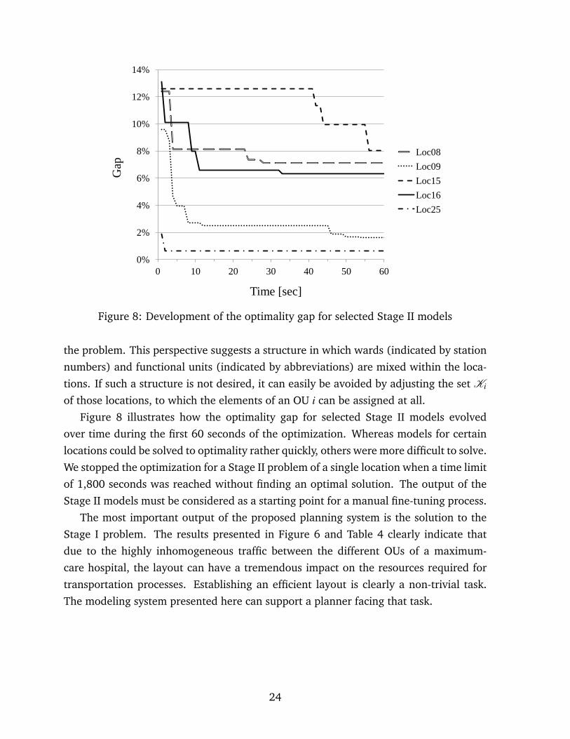
Figure 8 illustrates how the optimality gap for selected Stage II models evolved
over time during the first 60 seconds of the optimization. Whereas models for certain
locations could be solved to optimality rather quickly, others were more difficult to solve.
We stopped the optimization for a Stage II problem of a single location when a time limit
of 1,800 seconds was reached without finding an optimal solution. The output of the
Stage II models must be considered as a starting point for a manual fine-tuning process.
The most important output of the proposed planning system is the solution to the
Stage I problem. The results presented in Figure 6 and Table 4 clearly indicate that
due to the highly inhomogeneous traffic between the different OUs of a maximum-
care hospital, the layout can have a tremendous impact on the resources required for
transportation processes. Establishing an efficient layout is clearly a non-trivial task.
The modeling system presented here can support a planner facing that task.
24

6 Conclusion
We have analyzed and modeled the problem of assigning the different OUs of a large
maximum-care hospital within a given building structure that is sufficiently large to host
those units. We considered the space requirements and other real-world aspects with
the aim of obtaining a solution for the layout problem that minimizes the transportation
effort. To this end, we developed a hierarchical modeling system and a decomposition
algorithm that enabled us to solve problem instances with real-world characteristics de-
spite the computationally challenging underlying QAP. The computational burden of the
approach appears to be acceptable given the enormous planning effort to design such a
large maximum-care hospital. Although the proposed approach is neither intended nor
suited to fully automate the process of generating a solution for the layout problem, it
can systematically support this process.
References
Adams, W. P. and H. D. Sherali (1986). A Tight Linearization and an Algorithm for Zero-One
Quadratic Programming Problems. Management Science 32(10), 1274–1290.
Armour, G. C. and E. S. Buffa (1963). A Heuristic Algorithm and Simulation Approach to Relative
Location of Facilities. Management Science 9(2), 294–309.
Barbosa-Póvoa, A. P., R. Mateus, and A. Q. Novais (2001). Optimal two-dimensional layout of
industrial facilities. International Journal of Production Research 39(12), 2567–2593.
Barbosa-Póvoa, A. P., R. Mateus, and A. Q. Novais (2002). Optimal 3D layout of industrial
facilities. International Journal of Production Research 40(7), 1669–1698.
Böhme, D. (2013). Entwicklung von Entscheidungsmodellen für die innerbetriebliche Standortpla-
nung von Akutkrankenhäusern. Gottfried Wilhelm Leibniz Universität Hannover: Masterar-
beit, Institut für Produktionswirtschaft.
Bozer, Y. A. and R. D. Meller (1997). A reexamination of the distance-based facility layout
problem. IIE Transactions 29(7), 549–560.
Bozer, Y. A., R. D. Meller, and S. Erlebacher (1994). An Improvement-Type Layout Algorithm for
Single and Multiple-Floor Facilities. Management Science 40(7), 918–932.
Burkard, R. E., S. Karisch, and F. Rendl (1991). QAPLIB-A quadratic assignment problem library.
European Journal of Operational Research 55(1), 115–119.
Burkard, R. E. and J. Offermann (1977). Entwurf von Schreibmaschinentastaturen mittels
quadratischer Zuordnungsprobleme. Zeitschrift für Operations Research 21(4), 121–132.
Butler, T. W., K. R. Karwan, J. R. Sweigart, and G. R. Reeves (1992). An Integrative Model-Based
Approach to Hospital Layout. IIE Transactions 24(2), 144–152.
25

Drira, A., H. Pierreval, and S. Hajri-Gabouj (2007). Facility layout problems: A survey. Annual
Reviews in Control 31(2), 255–267.
Elshafei, A. N. (1977). Hospital Layout as a Quadratic Assignment Problem. Operational Research
Quarterly 28(1), 167–179.
Foulds, L. R. (1983). Techniques for Facilities Layout: Deciding Which Pairs of Activities Should
be Adjacent. Management Science 29(12), 1414–1426.
Garey, M. R. and D. S. Johnson (2009). Computers and intractability: A guide to the theory of
NP-completeness (27. print Aufl.). A series of books in the mathematical sciences. New York
NY u.a: Freeman.
Glover, F. and E. Woolsey (1974). Converting the 0-1 Polynomial Programming Problem to a
0-1 Linear Program. Operations Research 22(1), 180–182.
Hahn, P., J. MacGregor Smith, and Y.-R. Zhu (2010). The Multi-Story Space Assignment Prob-
lem. Annals of Operations Research 179(1), 77–103.
Hahn, P. M. and J. Krarup (2001). A hospital facility layout problem finally solved. Journal of
Intelligent Manufacturing 12, 487–496.
Hahn, P. M., Y.-R. Zhu, M. Guignard, W. L. Hightower, and M. J. Saltzman (2012). A Level-3
Reformulation-Linearization Technique-Based Bound for the Quadratic Assignment Prob-
lem. INFORMS Journal on Computing 24(2), 202–209.
Hassan, M. M. D. (1994). Machine layout problem in modern manufacturing facilities. Interna-
tional Journal of Production Research 32(11), 2559–2584.
Helber, S. and F. Sahling (2010). A fix-and-optimize approach for the multi-level capacitated lot
sizing problem. International Journal of Production Economics 123(2), 247–256.
Heragu, S. S. and A. Kusiak (1991). Efficient models for the facility layout problem. European
Journal of Operational Research 53(1), 1–13.
Hillier, F. S. and M. M. Connors (1966). Quadratic Assignment Problem Algorithms and the
Location of Indivisible Facilities. Management Science 13(1), 42–57.
Koopmans, T. C. and M. Beckmann (1957). Assignment Problems and the Location of Economic
Activities. Econometrica 25(1), 53–76.
Kusiak, A. and S. S. Heragu (1987). The facility layout problem. European Journal of Operational
Research 29(3), 229–251.
Levary, R. R. and S. Kalchik (1985). Facilities layout – a survey of solution procedures. Computers
& Industrial Engineering 9(2), 141–148.
Loiola, E. M., N. M. M. de Abreu, P. O. Boaventura-Netto, P. Hahn, and T. Querido (2007).
A survey for the quadratic assignment problem. European Journal of Operational Re-
search 176(2), 657 – 690.
Oral, M. and O. Kettani (1992). A Linearization Procedure for Quadratic and Cubic Mixed-
Integer Problems. Operations Research 40, 109–116.
26

Oucherif, F. (2012). Analyse und Optimierung der Layoutplanung von Krankenhäusern aus Sicht
der Transportlogistik durch Methoden des Operations Research. Gottfried Wilhelm Leibniz
Universität Hannover: Masterarbeit, Institut für Produktionswirtschaft.
Sahling, F. (2010). Mehrstufige Losgrößenplanung bei Kapazitätsrestriktionen. Gabler Research :
Produktion und Logistik. Wiesbaden: Gabler.
Steinberg, L. (1961). The Backboard Wiring Problem: A Placement Algorithm. SIAM Re-
view 3(1), 37–50.
Vos, L., S. Groothuis, and G. G. van Merode (2007). Evaluating hospital design from an opera-
tions management perspective. Health Care Management Science 10(4), 357–364.
27