A Gravity Gradient, Momentum-Biased Attitude Control ...
151
A GRAVITY GRADIENT, MOMENTUM-BIASED ATTITUDE CONTROL SYSTEM FOR A CUBESAT A Thesis presented to the Faculty of California Polytechnic State University, San Luis Obispo In Partial Fulfillment of the Requirements for the Degree Master of Science in Aerospace Engineering by Ryan Sellers March, 2013
Transcript of A Gravity Gradient, Momentum-Biased Attitude Control ...

A GRAVITY GRADIENT, MOMENTUM-BIASED ATTITUDE CONTROL SYSTEM
FOR A CUBESAT
A Thesis
presented to
the Faculty of California Polytechnic State University,
San Luis Obispo
In Partial Fulfillment
of the Requirements for the Degree
Master of Science in Aerospace Engineering
by
Ryan Sellers
March, 2013

Page ii
© 2013
Ryan Sellers
ALL RIGHTS RESERVED

Page iii
Committee Membership
TITLE: A Gravity Gradient, Momentum-Biased Attitude
Control System for a CubeSat
AUTHOR: Ryan Sellers
DATE SUBMITTED: March, 2013
COMMITTEE CHAIR: Dr. Eric Mehiel, Department Chair
Aerospace Engineering Department
COMMITTEE MEMBER: Dr. Jordi Puig-Suari, Professor
Aerospace Engineering Department
COMMITTEE MEMBER: Dr. Kira Abercromby, Professor
Aerospace Engineering Department
COMMITTEE MEMBER: Dr. John Bellardo, Professor
Computer Science Department
Page iv
Abstract
A Gravity Gradient, Momentum-Biased Attitude Control System for a CubeSat
Ryan Sellers
ExoCube is the latest National Science Foundation (NSF) funded space weather CubeSat
and is a collaboration between PolySat, Scientific Solutions Inc. (SSI), the University of
Wisconsin, NASA Goddard and SRI International. The 3U will carry a mass
spectrometer sensor suite, EXOS, in to low earth orbit (LEO) to measure neutral and
ionized particles in the exosphere and thermosphere. Measurements of neutral and ion
particles are directly impacted by the angle at which they enter EXOS and which leads to
pointing requirements. A combination of a gravity gradient system with a momentum
bias wheel is proposed to meet pointing requirements while reducing power requirements
and overall system complexity. A MATLAB simulation of dynamic and kinematic
behavior of the system in orbit is implemented to guide system design and verify that the
pointing requirements will be met. The problem of achieving the required three-axis
pointing is broken into four phases: detumbling, initial attitude acquisition, wheel spin-
up, and attitude maintenance. Ultimately, this configuration for attitude control in a
CubeSat could be applied to many future missions with the simulation serving as a design
tool for CubeSat developers.

Page v
Acknowledgements
I want to thank my friends, family, and girlfriend for all of their love and support. I also
want to acknowledge all of the work of those in the PolySat lab and CubeSat community
upon which my thesis is built on.

Page vi
Table of Contents
List of Tables ...................................................................................................................... x List of Figures .................................................................................................................... xi 1 Introduction ................................................................................................................. 1
1.1 Scope of Thesis ......................................................................................... 1
1.2 Background ............................................................................................... 1
1.2.1 CubeSat ............................................................................................... 1
1.2.2 ExoCube .............................................................................................. 3
2 Attitude Basics .......................................................................................................... 10 2.1 Reference Frames .................................................................................... 10
2.1.1 Earth Centered Inertial ...................................................................... 11
2.1.2 Earth Centered Earth Fixed ............................................................... 12
2.1.3 Geocentric Latitude, Longitude, Radius ........................................... 13
2.1.4 Perifocal ............................................................................................ 14
2.2.1 Orbital................................................................................................ 15
2.2.2 Body Fixed ........................................................................................ 16
2.3 Attitude Representations ......................................................................... 17
2.3.1 Direction Cosine Matrices ................................................................. 17
2.3.2 Euler Angles ...................................................................................... 19
2.3.3 Quaternions ....................................................................................... 22
3 Astrodynamics .......................................................................................................... 26 3.1 Kinematics ............................................................................................... 26
3.2 Dynamics ................................................................................................. 27
4 Space Environment ................................................................................................... 31 4.1 Earth Magnetic Field Model ................................................................... 31

Page vii
4.2 Sun Direction........................................................................................... 31
4.3 Eclipse Conditions................................................................................... 33
4.4 Atmospheric Model ................................................................................. 34
5 Environmental Disturbance Torques ........................................................................ 36 5.1 Gravity Gradient Torque ......................................................................... 36
5.1.1 Gravity Gradient Stability ................................................................. 37
5.2 Magnetic Torque ..................................................................................... 38
5.3 Aerodynamic Torque............................................................................... 39
5.4 Solar Radiation Pressure ......................................................................... 40
6 Attitude Determination & Control Architecture ....................................................... 42
6.1 Concept of Operations ............................................................................. 46
6.2 Attitude Determination ............................................................................ 47
6.3 Attitude Control Hardware ...................................................................... 49
6.3.1 Magnetorquers ................................................................................... 49
6.3.2 Momentum Wheel ............................................................................. 54
7 Attitude Control Algorithms ..................................................................................... 57
7.1 B-dot Detumbling Algorithm .................................................................. 57
7.1.1 Control Sequence .............................................................................. 58
7.2 Three-Axis Control Algorithm ................................................................ 59
7.2.1 Global Stability ................................................................................. 60
7.2.2 Gain Selection ................................................................................... 63
7.2.3 Moment of Inertia Uncertainty .......................................................... 64
7.2.4 Pseudo-Reverse Cross Product.......................................................... 65
7.2.5 Control Sequence .............................................................................. 65
8 Simulation and Results ............................................................................................. 67 8.1 Assumptions ............................................................................................ 67

Page viii
8.2 Satellite Specifications ............................................................................ 67
8.3 Guide to B-dot Controller Results Plots .................................................. 70
8.4 Detumbling .............................................................................................. 72
8.4.1 Gain Selection ................................................................................... 73
8.4.2 Pulse Time Selection ......................................................................... 78
8.4.3 Convergence Criteria Selection ......................................................... 81
8.4.4 Minimum Magnetometer Resolution ................................................ 82
8.4.5 Magnetometer Noise Tolerance ........................................................ 86
8.5 Guide to PD Controller Results Plots ...................................................... 87
8.6 Initial Attitude Acquisition...................................................................... 89
8.6.1 Gain Selection ................................................................................... 90
8.6.2 Pulse Time Selection ......................................................................... 94
8.6.3 Convergence Criteria......................................................................... 95
8.6.4 Orientation Error Tolerance .............................................................. 96
8.6.5 Angular Rate Error Tolerance ......................................................... 100
8.7 Wheel Spin Up ...................................................................................... 103
8.7.1 Wheel Spin Up Performance ........................................................... 106
8.7.2 Wheel Spin Up Performance with Torque Control Noise............... 107
8.8 Attitude Maintenance ............................................................................ 108
8.8.1 Reacquisition ................................................................................... 110
9 Conclusions ............................................................................................................. 111
10 Future Work ............................................................................................................ 115 10.1 Hardware in the loop ............................................................................. 115
10.2 Attitude Determination Algorithm ........................................................ 115
10.3 Pure Momentum Bias ............................................................................ 116

Page ix
References ....................................................................................................................... 117 APPENDIX A: B-dot Controller Gain Selection............................................................ 122 APPENDIX B: PD Controller Line Search for Optimal Gains ...................................... 130

Page x
List of Tables
Table 7.1: Summary of worst case environmental torques ............................................... 52
Table 9.1: Summary of Satellite Configurations for Simulation ...................................... 69
Table 9.2: Summary of B-dot controller results plots....................................................... 71
Table 9.3: Summary of PD controller results plots........................................................... 88
Table 10.1: Summary of detumbling performance ......................................................... 111
Table 10.2: Summary of ideal case initial acquisition performance ............................... 112
Table 10.3: Summary of Attitude Determination Algorithm Requirements .................. 113
Table 10.4: Summary of wheel spin up performance ..................................................... 113

Page xi
List of Figures
Figure 1.1: Distribution of Speeds for Gases (Brucat) ....................................................... 4
Figure 1.2: Half Angle Cone of Acceptance Definition ..................................................... 7
Figure 2.1: Earth Centered Inertial reference frame ......................................................... 11
Figure 2.2: Earth Centered Earth Fixed reference frame .................................................. 12
Figure 2.3: Geocentric Latitude, Longitude, Radius reference frame .............................. 13
Figure 2.4: Perifocal reference frame ............................................................................... 14
Figure 2.5: Orbital reference frame .................................................................................. 15
Figure 2.6: Body fixed reference frame ............................................................................ 16
Figure 2.7: Direction cosine transformation from xyz to x’y’z’ ....................................... 18
Figure 2.8: Classical Euler rotation sequence transforming xyz into x'y'z' ...................... 20
Figure 2.9: Yaw, pitch, and roll rotations transforming xyz into x'y'z' ............................ 21
Figure 2.10: Quaternion transformation from xyz to x'y'z' ............................................... 23
Figure 4.1: Components of Earth's Shadow (Eagle) ......................................................... 33
Figure 5.1: Illustration of the gravity gradient effect ........................................................ 36
Figure 5.2: The Smelt Parameter Plane (Hall) .................................................................. 38
Figure 6.1: Disturbance Torque Regimes (Turner) ........................................................... 44
Figure 6.2: Magnetorquer placement on ExoCube (highlighted in red) ........................... 51
Figure 6.3: Sinclair Interplanetary 10 mNm-sec Reaction Wheel .................................... 54
Figure 8.1: Panel representation of spacecraft in deployed configuration ........................ 68
Figure 8.2: B-dot performance for selected range of gains .............................................. 73
Figure 8.3: Optimal gain performance of the B-dot controller ......................................... 75
Figure 8.4: Sub-optimal gain performance of the B-dot controller .................................. 76
Page xii
Figure 8.5: Simulation depicting local instabilities of B-dot controller due to improper
gain selection ........................................................................................................ 77
Figure 8.6: B-dot performance for selected range of pulse times ..................................... 78
Figure 8.7: Simulation depicting instability of B-dot controller due to increased pulse
time ....................................................................................................................... 80
Figure 8.8: B-dot performance for range of selected convergence criteria ...................... 81
Figure 8.9: B-dot performance for range of magnetometer resolutions ........................... 82
Figure 8.10: Simulation depicting the impact of magnetometer resolution error on the B-
dot controller ......................................................................................................... 84
Figure 8.11: Simulation depicting the divergence of the B-dot controller due to
magnetometer resolution errors ............................................................................ 85
Figure 8.12: B-dot performance for range of magnetometer noise levels ........................ 86
Figure 8.13: Smelt parameter plane with deployed configuration plotted (indicated by red
X) .......................................................................................................................... 90
Figure 8.14: Optimal gain performance of PD controller for initial acquisition of the
target orientation ................................................................................................... 92
Figure 8.15: Sub-optimal gain performance of PD controller for initial acquisition of the
target orientation ................................................................................................... 93
Figure 8.16: PD controller performance for range of pulse times .................................... 94
Figure 8.17: Spacecraft pointing error for various initial angular rates ............................ 96
Figure 8.18: Simulation depicting the impact of quaternion resolution on the PD
controller ............................................................................................................... 98
Figure 8.19: Simulation depicting the impact of quaternion noise on the PD controller . 99

Page xiii
Figure 8.20: Simulation depicting the impact of rate resolution on the PD controller ... 101
Figure 8.21: Simulation depicting the impact of rate noise on the PD controller .......... 102
Figure 8.22: PD controller performance during wheel spin up ...................................... 106
Figure 8.23: PD controller performance during wheel spin up with noise in torque control
(𝝈 = 𝟏 × 𝟏𝟎 − 𝟔) ............................................................................................... 107
Figure 8.24: PD controller performance for reacquisition of pointing with torque control
noise (𝝈 = 𝟏 × 𝟏𝟎 − 𝟔) ...................................................................................... 110
Page 1
1 Introduction
1.1 Scope of Thesis
A combination of a gravity gradient system with a momentum bias wheel is proposed to
meet pointing requirements while reducing power requirements and overall system
complexity. A MATLAB simulation of dynamic and kinematic behavior of the system in
orbit is implemented to guide system design and verify that the pointing requirements
will be met. The problem is broken into four phases: detumbling, initial attitude
acquisition, wheel spin up, and attitude maintenance. Ultimately, this configuration for
attitude control in a CubeSat could be applied to many future missions with the
simulation serving as a design tool for CubeSat developers.
1.2 Background
1.2.1 CubeSat
For decades prior to the establishment of the CubeSat standard, universities saw the
potential in small satellites as a way to allow students to pursue research projects in
space, gain insight into satellite development, and experience the engineering design
cycle. Since the budget for most small satellite programs is orders of magnitude smaller
than that of industry satellite developers, ridesharing as a secondary payload on a launch
proved the most cost effective option. University small satellite programs faced the
challenges of the traditional secondary payload in trying to meet the requirements and

Page 2
schedule of a specific launch opportunity. Each program faced these challenges
individually and often lost launch opportunities due to incompatible requirements,
slippage in schedule, or prohibitive costs. These challenges led to longer development
cycles which in turn were lengthened more by the loss of institutional knowledge and
skill due to the high turnover rate of a university program with students graduating before
the completion of a project.
To overcome these challenges, the CubeSat standard was developed through the
collaboration of Dr. Jordi Puig-Suari of California Polytechnic State University San Luis
Obispo (Cal Poly) and Dr. Bob Twiggs of Stanford University in 1999 with the goal of
providing cost-effective access to space for university small satellite programs (CubeSat
Design Specification Rev. 12). The standard defines a CubeSat as a 10 cm cube with a
mass less than 1.33 kg with the purpose of being compatible with a common deployer
(CubeSat Design Specification Rev. 12). The CubeSat standard led to the establishment
of the student led CubeSat organization at Cal Poly which maintains the standard and
developed the Poly Picosatellite Orbital Deployer (P-POD). The P-POD is a flight proven
satellite deployment mechanism which can be interfaced with any launch vehicle.
Since the establishment of the standard, CubeSats have evolved from simple student
projects into fully capable small satellites which can greatly contribute to military,
commercial, and scientific space interests. The standard itself has evolved to include
larger CubeSats like the triple unit version known as the 3U. Although originally
perceived as too small to be capable of accomplishing meaningful missions, the order of

Page 3
magnitude lower cost and acceptance of the risk of commercial off-the-shelf (COTS)
parts has made CubeSats a viable solution.
Innovation in making smaller, lower power components driven by the cell phone industry
has led to dramatically smaller payloads that previously wouldn’t have fit within the
CubeSat form factor. Although the payloads are smaller, much of their inherited pointing
requirements remain the same, leading CubeSat developers to push the envelope for what
is possible in attitude determination and control on a CubeSat. Since CubeSats are
constrained in mass and volume which generally translates to power limitations, creative
attitude control techniques with low power requirements are needed to meet pointing
requirements while maximizing power available to the payload.
1.2.2 ExoCube
ExoCube is the latest National Science Foundation (NSF) funded space weather CubeSat
and is a collaboration between PolySat, Scientific Solutions Inc. (SSI), the University of
Wisconsin, NASA Goddard and SRI International. The 3U will carry a mass
spectrometer sensor suite, EXOS, in to low Earth orbit (LEO) to measure neutral and
ionized species in the exosphere and thermosphere. The EXOS payload will provide
valuable information to the space weather community and is the primary source of
pointing requirements for the proposed attitude control system.
Knowledge of upper atmospheric composition is essential to physics-based space weather
models. Current knowledge of atmospheric composition uses ground-based incoherent
scatter radar (ISR) which carries a higher level of inaccuracy as a result of the

Page 4
assumptions used when compared to in-situ mass spectroscopy methods. ExoCube will
provide the first in-situ global neutral density data since the era of the Dynamics Explorer
2 (DE-2) satellite (1981-1983), including the first direct measurements of exospheric
hydrogen using the mass spectrometer technique.
The EXOS sensor suite features a Static Energy-Angle-Analyzer (SEAA) that focuses
incident ion and neutral particles onto a Micro-Channel Plate (MCP) detector. Ions and
neutrals impact the MCP at different locations based on their velocity thus the SEAA
samples the velocity profile of the various gas species it is exposed to. Figure 1.1 is an
example of such a velocity profile showing the Maxwell-Boltzmann speed distribution of
gases (It should be noted that not all of these are the species of gases that will be in the
exosphere).
Figure 1.1: Distribution of Speeds for Gases (Brucat)
Page 5
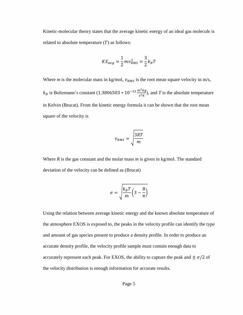
Kinetic-molecular theory states that the average kinetic energy of an ideal gas molecule is
related to absolute temperature (𝑇) as follows:
𝐾𝐸𝑎𝑣𝑔 =1
2𝑚𝑣𝑅𝑀𝑆
2 =3
2𝑘𝐵𝑇
Where m is the molecular mass in kg/mol, 𝑣𝑅𝑀𝑆 is the root mean square velocity in m/s,
𝑘𝐵 is Boltzmann’s constant (1.3806503 ∗ 10−23 𝑚2𝑘𝑔
𝑠2𝐾), and T is the absolute temperature
in Kelvin (Brucat). From the kinetic energy formula it can be shown that the root mean
square of the velocity is
𝑣𝑅𝑀𝑆 = √3𝑅𝑇
𝑚
Where R is the gas constant and the molar mass m is given in kg/mol. The standard
deviation of the velocity can be defined as (Brucat)
𝜎 = √𝑘𝐵𝑇
𝑚(3 −
8
𝜋)
Using the relation between average kinetic energy and the known absolute temperature of
the atmosphere EXOS is exposed to, the peaks in the velocity profile can identify the type
and amount of gas species present to produce a density profile. In order to produce an
accurate density profile, the velocity profile sample must contain enough data to
accurately represent each peak. For EXOS, the ability to capture the peak and ± 𝜎/2 of
the velocity distribution is enough information for accurate results.

Page 6
In order to accurately capture the velocity profiles of the various gas species in the
exosphere, EXOS is designed to be pointed in the ram direction in orbit to collect ions
and neutrals. If EXOS points slightly away from the ram direction, the angle at which the
ions and neutrals enter the SEAA is effected and thus the velocity profile becomes
skewed. The flux of particles entering the aperture of the SEAA becomes limited by the
cosine of the difference between the ram direction and the normal vector for the aperture.
Provided the offset between the aperture normal vector and the ram direction is a small
angle that is known through attitude determination, the loss in flux is minimal and the
velocity profile can be calibrated and still provide accurate results. However, if EXOS
points far enough off of the ram direction, only the high velocity molecules will be
collected thus producing a velocity profile that does not accurately represent all gas
species present. In order for the SEAA to have an accurate velocity profile, EXOS cannot
point outside a cone around the ram direction defined by the velocity of the slowest
molecule measured: atomic oxygen. The half angle of this cone of acceptance can be
defined by the triangle made by the spacecraft velocity vector (𝑣𝑆/𝐶) and the velocity of
vector of an atomic oxygen particle traveling in the cross track direction since it is the
widest angle possible for a molecule to make with respect to the spacecraft and still be
collected.

Page 7
Figure 1.2: Half Angle Cone of Acceptance Definition
Since an accurate representation of atomic oxygen requires capturing a sample of the
velocity distribution including the peak and ± 𝜎/2 of the curve, the 𝑣[𝑂] component of
the cone of acceptance should be
𝑣[𝑂] = 𝑣𝑅𝑀𝑆 −𝜎
2
Thus the half angle of the acceptance cone can be defined as
𝜃
2= tan−1 (
(𝑣𝑅𝑀𝑆 −𝜎2)
𝑣𝑆/𝐶)
ExoCube’s desired orbit is around 500 km altitude in the exobase portion of the
atmosphere where the median temperature varies with the solar cycle between 1000 and
1600 K. Given this range of expected temperatures and the kinetic energy relationship,
the following graph depicts the half angle required to capture the various gas species
sampled

Page 8
Figure 1.3: Half-Angle Acceptance Cone vs. Thermospheric Temperature (Gardner)
As can be seen in Figure 1.3, the half angle of acceptance for several of the expected gas
species are plotted. The solid and dashed lines represent the half angle of acceptance for
the range of temperatures for the root-mean-square velocity of each gas species and half
of a standard deviation of that velocity respectively. The equations used to generate these
lines are shown again on the graph for reference. The black dashed box represents the
source of the pointing accuracy requirement. The vertical elements of the black dashed
box represent the range of expected thermospheric temperatures while the horizontal
elements represent the intersection of the limiting case curves with the range of expected
temperatures. The limiting case of the acceptance cone for the range of expected
Page 9
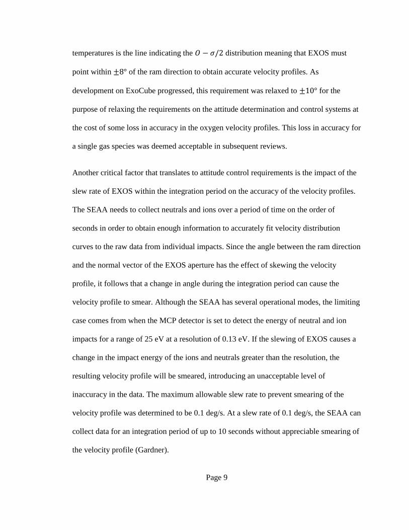
temperatures is the line indicating the 𝑂 − 𝜎/2 distribution meaning that EXOS must
point within ±8° of the ram direction to obtain accurate velocity profiles. As
development on ExoCube progressed, this requirement was relaxed to ±10° for the
purpose of relaxing the requirements on the attitude determination and control systems at
the cost of some loss in accuracy in the oxygen velocity profiles. This loss in accuracy for
a single gas species was deemed acceptable in subsequent reviews.
Another critical factor that translates to attitude control requirements is the impact of the
slew rate of EXOS within the integration period on the accuracy of the velocity profiles.
The SEAA needs to collect neutrals and ions over a period of time on the order of
seconds in order to obtain enough information to accurately fit velocity distribution
curves to the raw data from individual impacts. Since the angle between the ram direction
and the normal vector of the EXOS aperture has the effect of skewing the velocity
profile, it follows that a change in angle during the integration period can cause the
velocity profile to smear. Although the SEAA has several operational modes, the limiting
case comes from when the MCP detector is set to detect the energy of neutral and ion
impacts for a range of 25 eV at a resolution of 0.13 eV. If the slewing of EXOS causes a
change in the impact energy of the ions and neutrals greater than the resolution, the
resulting velocity profile will be smeared, introducing an unacceptable level of
inaccuracy in the data. The maximum allowable slew rate to prevent smearing of the
velocity profile was determined to be 0.1 deg/s. At a slew rate of 0.1 deg/s, the SEAA can
collect data for an integration period of up to 10 seconds without appreciable smearing of
the velocity profile (Gardner).

Page 10
2 Attitude Basics
The following sections will cover the basics of representing the orientation, or attitude, of
a rigid body by first establishing the reference frames used and then by summarizing the
methods of representing the relation between two frames.
2.1 Reference Frames
The following sections define the reference frames used in the simulation of the attitude
dynamics. The frames used follow the conventions found in most sources but it is
important to note that the orbital frame in particular varies between sources and the use of
a different convention will impact the results.

Page 11
2.1.1 Earth Centered Inertial
Figure 2.1: Earth Centered Inertial reference frame
The Earth-Centered Inertial (ECI) frame, also known as the geocentric equatorial frame,
is a non-rotating right handed Cartesian coordinate system with its origin at the center of
the Earth. The fundamental plane (𝑋𝐸𝐶𝐼, 𝑌𝐸𝐶𝐼) consists of the Earth’s equatorial plane
with the principal direction (𝑋𝐸𝐶𝐼) pointed at the first point of Aries (♈), the vernal
equinox. The right handed coordinate system is completed by 𝑍𝐸𝐶𝐼 which is orthogonal
to the Earth’s equatorial plane and coincides with the Earth’s axis of rotation (Curtis).

Page 12
2.1.2 Earth Centered Earth Fixed
Figure 2.2: Earth Centered Earth Fixed reference frame
The Earth Centered Equatorial Fixed (ECEF) frame rotates at the sidereal period of the
Earth with respect to the ECI frame with the origin at the center of the Earth. The
fundamental plane (𝑋𝐸𝐶𝐸𝐹, 𝑌𝐸𝐶𝐸𝐹), consists of the Earth’s equatorial plane with the
principal direction (𝑋𝐸𝐶𝐸𝐹) aligned with the intersection of the prime meridian and the
equator (0˚ Latitude, 0˚ Longitude). The right handed coordinate system is completed by
𝑍𝐸𝐶𝐸𝐹 which is orthogonal to the Earth’s equatorial plane and coincides with the Earth’s
axis of rotation (Curtis).

Page 13
2.1.3 Geocentric Latitude, Longitude, Radius
Figure 2.3: Geocentric Latitude, Longitude, Radius reference frame
The Geocentric Latitude, Longitude, and Radius (LLR) frame is the same as the ECEF
frame but is expressed in spherical coordinates instead of Cartesian coordinates. Latitude
is the angular measurement of North and South of the Equator (North is positive).
Longitude is the angular measurement East and West of the Prime Meridian (East is
positive). Radius is simply the distance from the center of the Earth to the position of
interest (Curtis).

Page 14
2.1.4 Perifocal
Figure 2.4: Perifocal reference frame
The Perifocal frame is an Earth centered, orbit based, inertial frame. The origin is
centered at the focus of the orbit; the center of the Earth. The fundamental plane (pq) is
the orbital plane with the principal direction (p) aligned with periapsis and q at 90˚ true
anomaly to p axis. The right handed coordinate system is completed by w which is
orthogonal to the orbital plane and aligned with the direction of the angular momentum
vector (Curtis).

Page 15
2.2.1 Orbital
Figure 2.5: Orbital reference frame
The Orbital frame is an Earth centered, orbit based, and rotating frame. The origin is
centered at the center of mass of the spacecraft with the 𝑋𝑂 axis pointing along the
position vector, opposite the center of the Earth (nadir). The 𝑍𝑂 axis is aligned with the
orbital angular momentum vector (cross-track). The right handed coordinate system is
completed by 𝑌𝑂 which is aligned with the velocity vector (in-track/ram) direction for
circular orbits (Kane, Likins and Levinson).

Page 16
2.2.2 Body Fixed
Figure 2.6: Body fixed reference frame
The Body Fixed (Body) frame is aligned geometrically with the spacecraft. The
orthogonal set of axes is defined with the origin at the geometric center of the 3U
structure with XBody, YBody, and ZBody axes normal to the sides of the CubeSat as in Figure
2.6. It should be noted that this differs from the coordinate system defined in the CubeSat
Design Specification and was done so to match the orbital reference frame and the
equations associated with it. Roll, Pitch, and Yaw are defined as rotations about the
XBody, YBody, and ZBody axes respectively.

Page 17
2.3 Attitude Representations
Representing a rigid body in three-dimensional space requires at least three parameters to
describe its orientation or attitude with respect to a reference frame. There are several
methods to mathematically represent the relationship between two frames. The following
section shall serve as an overview of the most common ones: direction cosine matrices
(DCM), Euler angles, and quaternions.
Before delving into the most common relationships between frames, it is important to
clarify the difference between a vector rotation and a vector transformation. A vector
rotation is an operation which changes the orientation of a vector in all coordinate frames.
A coordinate transform of a vector is an operation that describes a vector’s representation
with respect to a different coordinate frame than the original and does not change the
orientation of the vector (Groÿekatthöfer and Yoon 4).
2.3.1 Direction Cosine Matrices
A direction cosine matrix is a transformation matrix whose elements, the direction
cosines, describe the projection of the target coordinate system’s basis vectors onto an
initial coordinate system’s basis vectors. Given an initial frame A and a target frame B,
each defined by orthogonal unit basis vectors �̂�, 𝒋̂, and �̂�, we can express the target frame
in terms of the initial frame as follows:
�̂�𝑩 = 𝑄11 �̂�𝑨 + 𝑄12 𝒋̂𝑨 + 𝑄13 �̂�𝑨
𝒋̂𝑩 = 𝑄21 �̂�𝑨 + 𝑄22 𝒋̂𝑨 + 𝑄23 �̂�𝑨
�̂�𝑩 = 𝑄31�̂�𝑨 + 𝑄32 𝒋̂𝑨 + 𝑄33 �̂�𝑨

Page 18
Where the Q’s are the direction cosines of the basis vectors of B. Figure 2.7 illustrates the
components of �̂�𝑩 which are the projections of �̂�𝑩 onto �̂�𝑨, 𝒋̂𝑨, and �̂�𝑨 (Curtis 216).
Figure 2.7: Direction cosine transformation from xyz to x’y’z’
The DCM representing the transformation from frame A to frame B (𝑄𝐴𝐵) is an
orthonormal matrix because the basis vectors of both frames are orthogonal unit vectors.
Therefore the transpose of the DCM is the same as the DCM of the inverse
transformation:
𝑄𝐴𝐵𝑇 = 𝑄𝐴𝐵
−1 = 𝑄𝐵𝐴

Page 19
Transforming a vector in a frame A to frame B can be accomplished by the following
equation:
�⃗�𝐵 = 𝑄𝐴𝐵�⃗�𝐴
Successive transformations through intermediary frames can be accomplished by
multiplying successive DCMs as follows:
�⃗�𝐶 = 𝑄𝐵𝐶𝑄𝐴𝐵�⃗�𝐴
Note that the order by which the successive transformations are multiplied is right to left
starting with the transformation from the initial frame on the right and the transformation
to the final frame on the left.
The transformation of a coordinate frame about one of its basis vector through a rotation
angle 𝜃 can be described by the following primary transformation matrices:
𝑅1(𝜃) = [1 0 00 cos(𝜃) sin(𝜃)
0 − sin(𝜃) cos(𝜃)]
𝑅2(𝜃) = [cos(𝜃) 0 − sin(𝜃)
0 1 0sin(𝜃) 0 cos(𝜃)
]
𝑅3(𝜃) = [cos(𝜃) sin (𝜃) 0
−sin (𝜃) cos (𝜃) 00 0 1
]
R1, R2, and R3 correspond to rotations about the �̂�, 𝒋̂, and �̂� axes respectively
(Groÿekatthöfer and Yoon 4).
2.3.2 Euler Angles
The transformation between any two Cartesian coordinate frames can be thought of as a
sequence of three transformations using the primary transformation matrices R1, R2, and

Page 20
R3. The sequence of three transformations is called an Euler angle sequence. Since two
successive rotations cannot be about the same axis, there are twelve possible Euler angle
sequences. One of the sequences that is frequently used in space mechanics is the
classical Euler angle sequence:
𝑄𝐸𝑢𝑙𝑒𝑟 = 𝑅3(𝛾)𝑅1(𝛽)𝑅3(𝛼)
Figure 2.8: Classical Euler rotation sequence transforming xyz into x'y'z'
Another common Euler angle sequence in aerospace that is not to be confused with the
classical Euler angle sequence is the Yaw, Pitch, Roll (YPR) sequence (Curtis 224):
𝑄𝑌𝑃𝑅 = 𝑅1(𝑌𝑎𝑤)𝑅2(𝑃𝑖𝑡𝑐ℎ)𝑅3(𝑅𝑜𝑙𝑙)

Page 21
Figure 2.9: Yaw, pitch, and roll rotations transforming xyz into x'y'z'
The transformation of a vector via the classical Euler sequence or yaw-pitch-roll
sequence can be accomplished by applying the DCM for each sequence in the same
manner as the previous section.
Of all the possible different combinations of transformations, Euler angles and yaw-pitch-
roll representations of attitude are the most commonly used in graphical displays of
spacecraft orientation since they are relatively easy to interpret (Groÿekatthöfer and Yoon
5). However, when the nutation angle is 0 degrees in the classical Euler sequence or the
pitch angle is 90 degrees in the yaw-pitch-roll sequence, rotation axes align creating a
singularity. Thus Euler angle sequence representations are not effective in simulating
spacecraft kinematics.

Page 22
2.3.3 Quaternions
As mentioned in the previous section, Euler angle sequences cannot be relied upon for
modeling spacecraft kinematics due to the singularity problems. To avoid singularities
that arise from rotating about multiple and possibly aligned rotational axes, we refer to
Euler’s rotational theorem which states that the relative orientation of two coordinate
systems can be described by a unique rotation about a fixed axis through their common
origin. This axis of rotation is called the Euler eigenaxis and the angle is referred to as the
principal angle. In 1843, Irish mathematician Sir William R. Hamilton (1805-1865) used
Euler’s rotational theorem to introduce a practical alternative to DCMs: quaternions
(Curtis 554).
Quaternions are comprised of four elements. The vector component (�⃗�) is the first three
elements and the scalar component is the fourth (𝑞4). It is common to see the scalar
component as either the first or fourth element. The simulations and this paper will have
the scalar component as the fourth element as defined below:
𝑞 = [�⃗�𝑞4
] = [
𝑞1
𝑞2
𝑞3
𝑞4
]
All quaternions for attitude representations are unit quaternions, such that |𝑞| = 1. Thus
we can define them as:
𝑞 = [�⃗�𝑞4
] = [�̂� sin(𝜃)
cos(𝜃)]

Page 23
Where �̂� is the unit vector along the Euler axis around which the initial frame is rotated
into the target frame by the principal angle 𝜃 as shown in Figure 2.10 (Curtis 555).
Figure 2.10: Quaternion transformation from xyz to x'y'z'
The norm of a quaternion is
|𝑞| = √𝑞12 + 𝑞2
2 + 𝑞32 + 𝑞4
2
The conjugate quaternion has an inverted vector component

Page 24
𝑞∗ = [−�⃗�𝑞4
] = [
−𝑞1
−𝑞2
−𝑞3
𝑞4
]
The inverse of a quaternion is its normalized conjugate
𝑞−1 =𝑞∗
|𝑞|
It should be noted that since all of the quaternions dealt with are unit quaternions,
normalization is unnecessary and thus the inverse is the conjugate for unit quaternions.
The product of two quaternions 𝑞1 and 𝑞2 is defined by
𝑞1 ⊗ 𝑞2 = 𝑞 = [𝑣𝑠⃗⃗⃗
] = [𝑠1�⃗�2 + 𝑠2�⃗�1 + �⃗�1 × �⃗�2
𝑠1𝑠2 − �⃗�1 ⋅ �⃗�2]
Where �⃗� and 𝑠 are the vector and scalar components of the quaternions respectively.
Vector transformations using quaternions is defined as:
�⃗�𝐵 = 𝑞𝐴𝐵 ⊗ [�⃗�𝐴
0] ⊗ 𝑞𝐴𝐵
−1
Successive transformations through intermediary frames can be accomplished by
multiplying successive quaternions as follows:
𝑞𝐴𝐶 = 𝑞𝐴𝐵 ⊗ 𝑞𝐵𝐶
Note that the order by which the successive transformations are multiplied is left to right
(the opposite of successive DCMs) starting with the transformation from the initial frame

Page 25
on the left and the transformation to the final frame on the right (Groÿekatthöfer and
Yoon).

Page 26
3 Astrodynamics
3.1 Kinematics
The angular orientation of a spacecraft can be solved for in quaternions given a known
initial quaternion and angular rate with respect to the inertial frame using a numerical
differential equation solver on the following governing differential equation:
�̇⃗� =1
2[𝑞4𝜔𝑏𝑖 − 𝜔𝑏𝑖
× �⃗�]
�̇�4 = −1
2𝜔𝑏𝑖
𝑇 �⃗�
Where 𝜔𝑏𝑖 is the angular rate of the body with respect to the inertial frame and the
quaternion and its derivative also relate the body to the inertial frame (Curtis). The
superscript ×, as in 𝜔𝑏𝑖× , represents the skew-symmetric matrix known as the wedge
operator which performs the same function as the cross product as defined in the
following equation: (Curtis)
𝜔×�⃗� = 𝜔 × �⃗� = [
0 −𝜔3 𝜔2
𝜔3 0 −𝜔1
−𝜔2 𝜔1 0] �⃗�
The wedge operator is used in place of the cross product throughout the simulation as it is
more computationally efficient.

Page 27
3.2 Dynamics
Euler’s equation of rotational motion in homogeneous form states that the net moment
(𝑀𝑛𝑒𝑡) on a rigid body is equal to the absolute time derivative of its angular momentum
(𝐻)
𝑀𝑛𝑒𝑡 = �̇�
The absolute time derivative of the angular momentum is the sum of the change in
momentum relative to the co-moving frame and the cross product of the angular velocity
of the co-moving frame (Ω) and the momentum. As mentioned in section 3.1, the cross
product can be substituted for the wedge operator for the sake of computational
efficiency.
�̇� = �̇�𝑟𝑒𝑙 + Ω × 𝐻
= �̇�𝑟𝑒𝑙 + Ω×𝐻
For a co-moving frame rigidly attached to the body frame,
Ω = 𝜔
Given a constant moment of inertia (𝐼), the angular momentum and time derivative
become:
𝐻 = 𝐼𝜔
�̇�𝑟𝑒𝑙 = 𝐼�̇�

Page 28
Thus Euler’s equation can be rewritten as
𝑀𝑛𝑒𝑡 = 𝐼�̇� + 𝜔×𝐼𝜔
If we add 𝑛 reaction wheels, the total angular momentum become
𝐻𝑎𝑏𝑠 = 𝐻𝑏𝑜𝑑𝑦𝑐𝑔
+ ∑ 𝐻𝑤ℎ𝑒𝑒𝑙(𝑖)𝑐𝑔𝑛
𝑖=1
Where 𝐻𝑏𝑜𝑑𝑦𝑐𝑔
is the angular momentum of the body without wheels around the center of
gravity (𝑐𝑔) of the body and the second term is the sum of the angular momentum of each
wheel about the 𝑐𝑔 of the body. Given constant moments of inertia for the body and the
wheels the angular momentum can be rewritten as
𝐻𝑎𝑏𝑠 = 𝐼𝑏𝑜𝑑𝑦𝑐𝑔
𝜔 + ∑ (𝐼𝑤ℎ𝑒𝑒𝑙(𝑖)𝑐𝑔(𝑖)
𝜔𝑤ℎ𝑒𝑒𝑙(𝑖)𝑎𝑏𝑠 + 𝐼𝑤ℎ𝑒𝑒𝑙(𝑖)
𝑐𝑔𝜔)
𝑛
𝑖=1
Where 𝐼𝑤ℎ𝑒𝑒𝑙(𝑖)𝑐𝑔(𝑖)
is the moment of inertia of reaction wheel 𝑖 with respect to its own center
of gravity 𝑐𝑔(𝑖) while 𝐼𝑤ℎ𝑒𝑒𝑙(𝑖)𝑐𝑔
is the moment of inertia of the same wheel with respect to
the 𝑐𝑔 of the main body. Also, 𝜔 is the angular rate of the body and 𝜔𝑤ℎ𝑒𝑒𝑙(𝑖)𝑎𝑏𝑠 is the
angular rate of reaction wheel 𝑖 with respect to the inertial frame. The two rates are
related by
𝜔𝑤ℎ𝑒𝑒𝑙(𝑖)𝑎𝑏𝑠 = 𝜔𝑤ℎ𝑒𝑒𝑙(𝑖) + 𝜔
Where 𝜔𝑤ℎ𝑒𝑒𝑙(𝑖) is the angular rate of the wheel relative to the body frame. Using this
relation and rearranging we obtain

Page 29
𝐻𝑎𝑏𝑠 = (𝐼𝑏𝑜𝑑𝑦𝑐𝑔
+ ∑ 𝐼𝑤ℎ𝑒𝑒𝑙(𝑖)𝑐𝑔
𝑛
𝑖=1
) 𝜔 + ∑(𝐼𝑤ℎ𝑒𝑒𝑙(𝑖)𝑐𝑔(𝑖)
𝜔𝑤ℎ𝑒𝑒𝑙(𝑖))
𝑛
𝑖=1
The sum of the moments of inertia in the first term constitute the total moment of inertia
for the spacecraft (𝐼𝑡𝑜𝑡𝑎𝑙) as follows
𝐼𝑡𝑜𝑡𝑎𝑙 = 𝐼𝑏𝑜𝑑𝑦𝑐𝑔
+ ∑ 𝐼𝑤ℎ𝑒𝑒𝑙(𝑖)𝑐𝑔
𝑛
𝑖=1
To simplify notation 𝐼𝑤ℎ𝑒𝑒𝑙(𝑖)𝑐𝑔(𝑖)
can be written as 𝐼𝑤ℎ𝑒𝑒𝑙(𝑖) and thus the absolute angular
momentum can be rewritten as
𝐻𝑎𝑏𝑠 = 𝐼𝑡𝑜𝑡𝑎𝑙𝜔 + ∑(𝐼𝑤ℎ𝑒𝑒𝑙(𝑖)𝜔𝑤ℎ𝑒𝑒𝑙(𝑖))
𝑛
𝑖=1
Taking the time derivative we find
�̇�𝑟𝑒𝑙 = 𝐼𝑡𝑜𝑡𝑎𝑙�̇� + ∑(𝐼𝑤ℎ𝑒𝑒𝑙(𝑖)�̇�𝑤ℎ𝑒𝑒𝑙(𝑖))
𝑛
𝑖=1
Where �̇�𝑤ℎ𝑒𝑒𝑙(𝑖) is the relative angular acceleration of wheel 𝑖. Plugging these back in to
Euler’s equation for rotational motion gives us
𝑀𝑛𝑒𝑡 = 𝐼𝑡𝑜𝑡𝑎𝑙�̇� + ∑(𝐼𝑤ℎ𝑒𝑒𝑙(𝑖)�̇�𝑤ℎ𝑒𝑒𝑙(𝑖))
𝑛
𝑖=1
+ 𝜔× (𝐼𝑡𝑜𝑡𝑎𝑙𝜔 + ∑(𝐼𝑤ℎ𝑒𝑒𝑙(𝑖)𝜔𝑤ℎ𝑒𝑒𝑙(𝑖))
𝑛
𝑖=1
)
Rearranging to obtain the differential equation for the numerical solver for the simulation
we obtain (Curtis 617)

Page 30
�̇� = 𝐼𝑡𝑜𝑡𝑎𝑙−1 (𝑀𝑛𝑒𝑡 − ∑(𝐼𝑤ℎ𝑒𝑒𝑙(𝑖)�̇�𝑤ℎ𝑒𝑒𝑙(𝑖))
𝑛
𝑖=1
− 𝜔× (𝐼𝑡𝑜𝑡𝑎𝑙𝜔 + ∑(𝐼𝑤ℎ𝑒𝑒𝑙(𝑖)𝜔𝑤ℎ𝑒𝑒𝑙(𝑖))
𝑛
𝑖=1
))

Page 31
4 Space Environment
4.1 Earth Magnetic Field Model
An accurate model of the Earth’s magnetic field is necessary to model the input to
magnetometers as well as model magnetic torques. The International Geomagnetic
Reference Field (IGRF) was introduced by the International Association of
Geomagnetism and Aeronomy (IAGA) in 1968 as a standard spherical harmonic
representation of the Earth’s main field that is updated every five years and is available at
http://www.ngdc.noaa.gov/IAGA/vmod/. The model has a precision of 0.1 nano-Teslas
per year (IGRF Guide). This simulation uses the MATLAB code magfd.m created by
Maurice A. Tivey of the Woods Hole Oceanographic Institution to compute the Earth’s
magnetic field components using the IGRF-10 model.
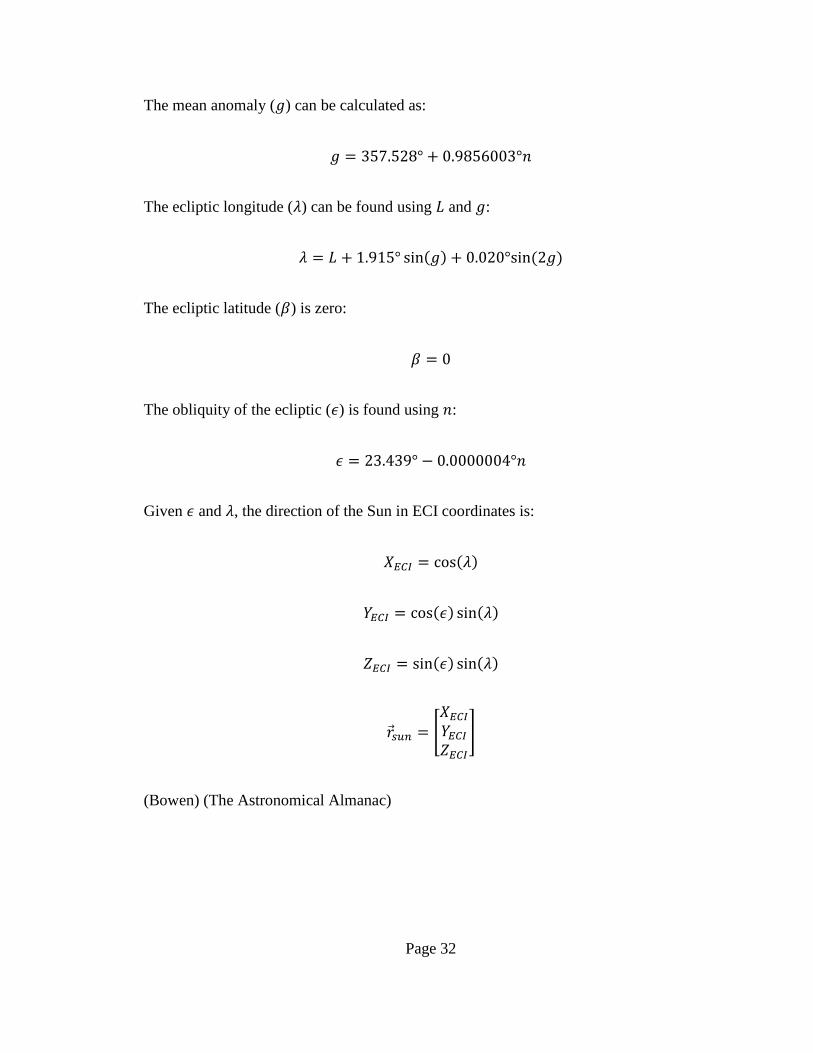
4.2 Sun Direction
The direction of the Sun in ECI coordinates are necessary for simulating the input to sun
sensors and solar radiation pressure. The Astronomical Almanac provides formulas for
computing the Sun’s position to within a precision of 0.01°. The following formulas
outline the method provided by the Astronomical Almanac:
The number of days since J2000.0 (𝑛) is calculated from the Julian Date (𝐽𝐷)
𝑛 = 𝐽𝐷 − 2451545.0
The mean longitude of the Sun in degrees (𝐿) is given as:
𝐿 = 280.460° + 0.9856474°𝑛
Page 32
The mean anomaly (𝑔) can be calculated as:
𝑔 = 357.528° + 0.9856003°𝑛
The ecliptic longitude (𝜆) can be found using 𝐿 and 𝑔:
𝜆 = 𝐿 + 1.915° sin(𝑔) + 0.020°sin (2𝑔)
The ecliptic latitude (𝛽) is zero:
𝛽 = 0
The obliquity of the ecliptic (𝜖) is found using 𝑛:
𝜖 = 23.439° − 0.0000004°𝑛
Given 𝜖 and 𝜆, the direction of the Sun in ECI coordinates is:
𝑋𝐸𝐶𝐼 = cos(𝜆)
𝑌𝐸𝐶𝐼 = cos(𝜖) sin(𝜆)
𝑍𝐸𝐶𝐼 = sin(𝜖) sin(𝜆)
𝑟𝑠𝑢𝑛 = [
𝑋𝐸𝐶𝐼
𝑌𝐸𝐶𝐼
𝑍𝐸𝐶𝐼
]
(Bowen) (The Astronomical Almanac)

Page 33
4.3 Eclipse Conditions
Modeling the satellite’s entrance and exit into the Earth’s shadow is important to accurate
modeling of the solar radiation pressure torques. Due to the Sun’s size and proximity to
Earth, it should not be treated as a point source and therefore has a distinct umbra and
penumbra parts of its shadow as shown in Figure 4.1.
Figure 4.1: Components of Earth's Shadow (Eagle)
To calculate the various parts of Earth’s shadow, one must first calculate the half angle
the cylindrical projection of the Earth (𝜃𝐶) at the satellite’s distance from the Earth in
orbit 𝑟𝑠𝑎𝑡.
𝜃𝐶 = sin−1 (𝑅𝐸
‖𝑟𝑠𝑎𝑡‖)

Page 34
Where 𝑅𝐸 is the Earth’s radius. For more realistic shadow predictions, the radius of the
Earth has been increased by 2% to account for the effect of the Earth’s atmosphere on the
size of the shadow. The half angle of Earth’s umbra (𝜃𝑈) can be calculated as
𝜃𝑈 = sin−1 (𝑑𝑠𝑢𝑛 − 𝑅𝐸
‖𝑟𝑠𝑢𝑛‖) − 𝜃𝐶
Where 𝑑𝑠𝑢𝑛 is the radius of the sun. Similarly, the Earth’s penumbra can be calculated as
𝜃𝑃 = sin−1 (𝑑𝑠𝑢𝑛 + 𝑅𝐸
‖𝑟𝑠𝑢𝑛‖) − 𝜃𝐶
The location of Earth’s shadow can be defined by the negative of the Sun direction vector
in ECI, the shadow axis
�̂�𝑠ℎ𝑎𝑑𝑜𝑤 = −𝑟𝑠𝑢𝑛
‖𝑟𝑠𝑢𝑛‖
The angle of the satellite relative to the shadow axis can be defined as (Eagle)
𝜙 = cos−1(�̂�𝑠ℎ𝑎𝑑𝑜𝑤 ∙ �̂�𝑠𝑎𝑡)
4.4 Atmospheric Model
An accurate model of atmospheric density is required to model the aerodynamic torques
on the spacecraft. The US Naval Research Laboratory’s (NRL) Mass Spectrometer and
Incoherent Scatter Radar Exosphere (MSISE) model is an empirical, global model of the
Earth’s atmosphere that spans from sea level to the exosphere. The model calculates
composition, temperature, and total mass density. The current model released in 2000,
NRLMSISE-00, incorporates the main drivers for the upper atmosphere above 75 km; the

Page 35
10.7 cm solar radio flux (𝐹10.7) and the daily geomagnetic index (𝐴𝑝) (Picone, Drob and
Meier). For this simulation, the solar flux and magnetic indices are obtained from
ftp.ngdc.noaa.gov using a MATLAB code f107_aph.m created by John A. Smith of
CIRES/NOAA that is available online (Smith). Not only does this model serve as a
reference for the atmospheric density to model aerodynamic torques on the spacecraft,
but will also directly benefit from the data gathered by EXOS.

Page 36
5 Environmental Disturbance Torques
5.1 Gravity Gradient Torque
An asymmetric body subject to a gravitational field will experience a torque tending to
align the axis of least inertia with the field direction (Sidi 108).
Figure 5.1: Illustration of the gravity gradient effect
According to Newton’s Law of Universal Gravitation, in a central gravitational field,
portions of a body closer to earth are attracted more strongly than portions further away.
Although this force is relatively weak, for an object in LEO, it can be enough to stabilize
a satellite to be nadir pointing (Schaub and Junkins). The moon is one example of a
naturally gravity gradient stable system. Because the moon has a slight elongation, the
same face of the moon points towards the earth as it rotates around it in its orbit (Stern).
The gravity gradient torque can be written as (B. Wie 388)

Page 37
𝑇𝑔𝑔 = 3𝑛2𝑜1 × (𝐼𝑡𝑜𝑡𝑎𝑙𝑜1)
Where n is the mean motion of the satellite and 𝑜1 is the basis vector of the orbital frame
that is aligned with the orbital position vector and thus the general gravity field defined
with respect to the body frame taken from the first column of the direction cosine matrix
for the body to orbital transformation 𝑄𝑏𝑜.
5.1.1 Gravity Gradient Stability
By solving the dynamics equations with the gravity gradient torque and assuming an
exponential solution, the characteristic equation leads to a set of 3 inertia parameters
known as the Smelt parameters and are bounded between ±1 (Hall)
𝐾𝑟𝑜𝑙𝑙 =𝐼𝑝𝑖𝑡𝑐ℎ − 𝐼𝑦𝑎𝑤
𝐼𝑟𝑜𝑙𝑙
𝐾𝑝𝑖𝑡𝑐ℎ =𝐼𝑟𝑜𝑙𝑙 − 𝐼𝑦𝑎𝑤
𝐼𝑝𝑖𝑡𝑐ℎ
𝐾𝑦𝑎𝑤 =𝐼𝑝𝑖𝑡𝑐ℎ − 𝐼𝑟𝑜𝑙𝑙
𝐼𝑦𝑎𝑤
The four stability conditions can be expressed as (Hall)
𝐶𝑜𝑛𝑑𝑖𝑡𝑖𝑜𝑛 𝐼: 𝐾𝑟𝑜𝑙𝑙 > 𝐾𝑦𝑎𝑤
𝐶𝑜𝑛𝑑𝑖𝑡𝑖𝑜𝑛 𝐼𝐼: 𝐾𝑟𝑜𝑙𝑙 ∙ 𝐾𝑦𝑎𝑤 > 0
𝐶𝑜𝑛𝑑𝑖𝑡𝑖𝑜𝑛 𝐼𝐼𝐼: 1 + 3𝐾𝑟𝑜𝑙𝑙 + 𝐾𝑟𝑜𝑙𝑙 ∙ 𝐾𝑦𝑎𝑤 > 0
𝐶𝑜𝑛𝑑𝑖𝑡𝑖𝑜𝑛 𝐼𝑉: (1 + 3𝐾𝑟𝑜𝑙𝑙 + 𝐾𝑟𝑜𝑙𝑙 ∙ 𝐾𝑦𝑎𝑤)2
− 16𝐾𝑟𝑜𝑙𝑙 ∙ 𝐾𝑦𝑎𝑤 > 0

Page 38
Using these conditions, one can construct the stability diagram for a gravity gradient
system known as the Smelt Parameter Plane. The conditions bound the stable
configurations to exist within the Lagrange and Debra-Delp (D2) regions.
Figure 5.2: The Smelt Parameter Plane (Hall)
5.2 Magnetic Torque
The interaction between the magnetic moment (𝑀) produced within a spacecraft and the
Earth’s magnetic field (𝐵) creates a torque (𝑇𝑚𝑎𝑔) that can be used for actuation that is
the cross product of the two (Sidi 185).
𝑇𝑚𝑎𝑔 = 𝑀 × 𝐵

Page 39
Because 𝑇𝑚𝑎𝑔 is the result of a cross product and is therefore always perpendicular to the
magnetic field vector 𝐵, the satellite can only be actuated in the two axes perpendicular
to the current magnetic field vector. Although only two axes are controllable at any given
time in orbit, the spacecraft experiences two full rotations of the earth’s magnetic field
vector per orbit making all axes controllable over time. Controllability is also limited
since 𝑇𝑚𝑎𝑔 is proportional to the magnitude of the earth magnetic field vector (Wertz
113).
5.3 Aerodynamic Torque
Atmospheric density exhibits an overall trend of exponential decay as a function of
altitude making torques due to aerodynamic drag a concern mainly for LEO spacecraft.
At altitudes that can be qualified as LEO and above, the atmosphere is rarefied and thus
the forces created by impacting an object in orbit can be modeled as particles. A
simplified model of the torque on a flat panel produced by aerodynamic drag can be
written as: (Wertz) (Varma)
𝑇𝑎𝑒𝑟𝑜 =1
2𝜌𝐶𝐷𝐴𝑝‖�⃗�𝑟𝑒𝑙‖
2𝑣𝑟𝑒𝑙 × 𝑟𝑐𝑝
Where 𝜌 is the atmospheric density in kg/m3, 𝐶𝑑 is the unitless coefficient of drag
(typically between 2 and 2.5 for LEO spacecraft), �̂� is the outward normal unit vector of
the panel, and 𝑟𝑐𝑝 is the vector from the center of mass of the S/C to the center of
aerodynamic pressure. �⃗�𝑟𝑒𝑙 is the velocity vector of the spacecraft in km/s. The projected
area (𝐴𝑝) in the equation above can be calculated as

Page 40
𝐴𝑝 = 𝐴 cos (𝛾)
Where 𝐴 is the surface are of the panel in m2 and 𝛾 is the angle between the normal
vector of the panel (�̂�) and the relative velocity of the spacecraft (�⃗�𝑟𝑒𝑙). The angle 𝛾 can
be calculated as
𝛾 = acos (�̂� ∙ �⃗�𝑟𝑒𝑙
‖�̂�‖ ‖�⃗�𝑟𝑒𝑙‖)
The relative velocity (�⃗�𝑟𝑒𝑙) of the spacecraft in the body frame takes into account the
rotation of Earth’s atmosphere and can be approximated as
�⃗�𝑟𝑒𝑙 = [1 − 𝜔𝐸
‖𝑟‖
‖�⃗�‖cos(𝑖)] �⃗�
Where 𝑟 and �⃗� are the satellite position and velocity in the body frame respectively, 𝜔𝐸 is
the angular rate of rotation of the Earth, and 𝑖 is the orbital inclination (Varma).
5.4 Solar Radiation Pressure
The light and radiation emitted by the sun has momentum that exerts pressure on objects
exposed to it. The amount of momentum from the solar radiation that is reflected and
absorbed is dependent on material properties and can be quantified by the reflectance
factor (q), a unitless measure ranging from 0 for perfect absorption to 1 for perfect
reflection. A simplified model of the torque on a flat panel produced by solar radiation
pressure (SRP) can be written as: (Wertz, Everett and Puschell 571)
𝑇𝑆𝑅𝑃 =𝜙
𝑐𝐴𝑝(1 + 𝑞)�̂�𝑇�⃗�𝑠𝑢𝑛(�⃗�𝑠𝑢𝑛 × 𝑠𝑐𝑝)

Page 41
Where 𝜙 is the solar output at 1 AU (1366 W/m2), c is the speed of light in a vacuum
(2.99792458*108 m/s), A is the surface area in m2, �̂� is the outward normal unit vector for
the panel modeled, �⃗�𝑠𝑢𝑛 is the sun direction in body coordinates, and 𝑠𝑐𝑝 is the vector
from the center of mass of the S/C to the center of solar pressure on the panel (which is
assumed to be the same as the center of aerodynamic pressure for these simulations).

Page 42
6 Attitude Determination & Control Architecture
The attitude determination and control (ADC) architecture of a CubeSat is limited
primarily by two considerations: budget and power. The budget drives the design because
while the NSF space weather grant awarded to ExoCube is one of the larger sources of
funding available to university CubeSats, it is still orders of magnitude lower than that of
a typical commercial satellite. The power availability drives the design because the mass
and volume constraints of the CubeSat standard inherently limit the ability to generate
and store power forcing developers to seek out low power active or passive attitude
control architectures in order to meet pointing requirements and maximize power
available to the payload.
ExoCube needs to maintain pointing in the ram direction within ±10° with angular rates
less than 0.01 deg/s during science modes. The requirement to point in the ram direction
with a relative small angular rate rules out the purely passive options and indicates the
need for three-axis pointing. The most common fully active solutions for CubeSats use
magnetorquers and reaction wheels for precise three-axis pointing. Magnetorquers create
a dipole calculated to exert a torque against the earth magnetic field to actuate the
satellite. An active magnetic system requires at least three orthogonal magnetorquers and
can achieve accuracies of approximately ±1° depending on the attitude knowledge
(Wertz, Everett and Puschell 574). However, operation of the magnetorquers to
continuously maintain pointing would draw excessive power and interfere with the flux
of ions into EXOS. Reaction wheels are torque motors with high inertia rotors that can be
spun to actuate a satellite (Wertz, Everett and Puschell 579). A zero momentum system

Page 43
uses at least 3 orthogonal reaction wheels to actuate a satellite to accuracies of ±1° and
below using alternative actuators like magnetorquers to dump any built up momentum in
the wheels (Wertz, Everett and Puschell 574). Although a potentially very accurate agile
system, commercial off the shelf (COTS) options for the minimum three reaction wheels
required for a zero momentum system are cost prohibitive and draw excessive power. By
selecting an over capable attitude control system the developer assumes a lot of
unnecessary complexity and cost that ultimately takes away from the primary mission if
it doesn’t make it entire infeasible. Upon re-examination, ExoCube’s pointing
requirements are relatively modest in comparison to the capabilities of these fully active
three axis control systems and suggest a combination of passive and active elements as
the solution.
With power and budget considerations in mind, the design approach for the ADC
architecture was to begin with what could be achieved by a purely passive system and
then add active elements to tailor a solution to meet the requirements. The passive
solutions considered were: permanent magnets, aerodynamically stabilized, and gravity
gradient stabilized. A permanent magnet system will align a spacecraft in a polar orbit
with the ram direction but was ruled out because the system will flip at the poles and the
permanent magnet will interfere with the flux of ionized particles and operation of
EXOS. An aerodynamically stabilized system will align with the ram direction providing
stability for yaw and pitch motion but roll motion is uncontrolled. A gravity gradient
stabilized system will align with the nadir direction providing stability for pitch and roll
motion but yaw motion is uncontrolled. Figure 6.1 is a comparison of environmental

Page 44
torques by altitude and illustrates that gravity gradient torques dominate aerodynamic
torques above an altitude of 400 km. Since the desired orbital regime for ExoCube is
between 425 and 650 km in the thermosphere and lower exosphere, a gravity gradient
stabilized system was selected.
Figure 6.1: Disturbance Torque Regimes (Turner)
Although a 3U CubeSat with evenly distributed mass is technically gravity gradient
stable by the Smelt parameters defined previously, the addition of deployable booms with
mass concentrated at the end maximizes the moment of inertia and more importantly
makes the center of gravity and alignment of the principal axes and the body axes less
sensitive to misalignment errors. Deploying the booms symmetrically from the top and
bottom of the 3U (+/- z panels) aids in keeping the system aerodynamically balanced by

Page 45
keeping the center of pressure close to the center of mass, avoiding the inherent offset in
pointing that would be caused by a single boom deployment.
As mentioned previously, a gravity gradient stabilized system has uncontrolled yaw
motion. In order to point EXOS in the ram direction, an active control element is
required. Since the use of magnetorquers would interfere with EXOS, the gravity gradient
system was combined with a momentum bias system.
A momentum bias system can point in the ram direction within ±1° or better by utilizing
a momentum wheel mounted in the pitch axis. The momentum wheel runs at a near
constant speed for gyroscopic stability in the roll and yaw disturbances while maintaining
pointing in the pitch axis by torqueing the wheel, slightly increasing or decreasing its
speed. However, a pure momentum bias system would require periodic momentum
dumping, causing frequent interruptions to the operation of EXOS (Wertz, Everett and
Puschell 577). By combining a momentum bias with a gravity gradient system, the need
for active pitch control and periodic momentum dumping is unnecessary since the gravity
gradient system is already stable for pitch motion and the momentum bias will reject
disturbances causing yaw drift. The gravity gradient, momentum bias system will still
require active magnetic control using magnetorquers for detumbling, initial acquisition of
the nominal orientation, wheel spin-up, and re-acquisition of the nominal orientation
should ExoCube drift outside its pointing requirements.
Page 46
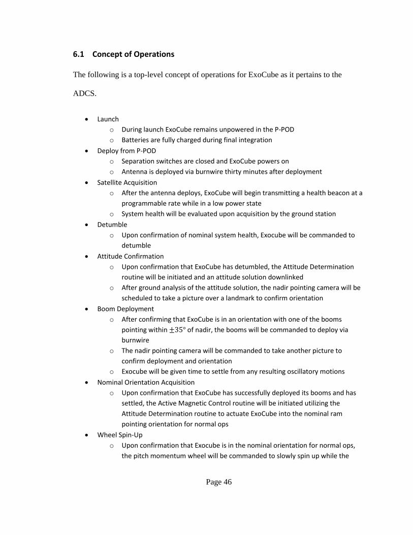
6.1 Concept of Operations
The following is a top-level concept of operations for ExoCube as it pertains to the
ADCS.
Launch
o During launch ExoCube remains unpowered in the P-POD
o Batteries are fully charged during final integration
Deploy from P-POD
o Separation switches are closed and ExoCube powers on
o Antenna is deployed via burnwire thirty minutes after deployment
Satellite Acquisition
o After the antenna deploys, ExoCube will begin transmitting a health beacon at a
programmable rate while in a low power state
o System health will be evaluated upon acquisition by the ground station
Detumble
o Upon confirmation of nominal system health, Exocube will be commanded to
detumble
Attitude Confirmation
o Upon confirmation that ExoCube has detumbled, the Attitude Determination
routine will be initiated and an attitude solution downlinked
o After ground analysis of the attitude solution, the nadir pointing camera will be
scheduled to take a picture over a landmark to confirm orientation
Boom Deployment
o After confirming that ExoCube is in an orientation with one of the booms
pointing within ±35° of nadir, the booms will be commanded to deploy via
burnwire
o The nadir pointing camera will be commanded to take another picture to
confirm deployment and orientation
o Exocube will be given time to settle from any resulting oscillatory motions
Nominal Orientation Acquisition
o Upon confirmation that ExoCube has successfully deployed its booms and has
settled, the Active Magnetic Control routine will be initiated utilizing the
Attitude Determination routine to actuate ExoCube into the nominal ram
pointing orientation for normal ops
Wheel Spin-Up
o Upon confirmation that Exocube is in the nominal orientation for normal ops,
the pitch momentum wheel will be commanded to slowly spin up while the

Page 47
Active Magnetic Control routine maintains position and opposes the torques
from the wheel
o ExoCube’s orientation is confirmed again by the nadir pointing camera
Begin Normal Ops
o Upon confirmation of nominal orientation and momentum wheel at speed,
ExoCube will begin Normal Ops
Attitude Maintenance
o Upon analysis of downlinked attitude solutions and determination that ExoCube
has drifted outside of its pointing requirements for nominal orientation, the
command to suspend Normal Ops will be uplinked.
o The pitch momentum wheel will be commanded to slowly despin while the
Active Magnetic Control routine maintains position and opposes the torques
from the wheel.
o The Active Magnetic Control routine reacquires the nominal ram pointing
orientation.
o The wheel will be commanded to spin up slowly while the Active Magnetic
Control routine maintains position and opposes the torques from the wheel.
o ExoCube’s orientation is confirmed again by the nadir pointing camera
o Upon confirmation that ExoCube is in the nominal orientation, Normal Ops will
be commanded to resume
6.2 Attitude Determination
Full three-axis control requires full knowledge of spacecraft orientation and rotational
rates. A complete attitude solution requires a suite of sensors that measure rotation rates
and use external references to find the spacecraft’s orientation. Magnetometers and sun
sensors are common solutions used by CubeSat developers and have been selected for
ExoCube based largely off of their cost relative to other commercial off the shelf
solutions suitable for CubeSats.
Magnetometers measure the magnitude and direction of the Earth’s magnetic field
relative to the spacecraft and can provide its orientation relative to the inertial frame in
two axes when combined with knowledge of the spacecraft’s orbital position and the
local magnetic field. They are required by the magnetorquers in order to calculate the

Page 48
required magnetic dipole to execute commanded torques from the control algorithm.
Magnetometers in general have relatively low internal noise but are sensitive to
electromagnetic interference from the onboard electronics. As a result, the
magnetometers will be placed on the deployable gravity gradient booms to take
advantage of the distance from the electromagnetic interference of the main avionics. To
simulate the error contribution of magnetometer resolution and noise from the spacecraft
electronics, the following equation is used:
𝑏𝑚𝑒𝑎𝑠 = 𝑟𝑜𝑢𝑛𝑑(𝑏𝑒𝑥𝑎𝑐𝑡 + 𝜎𝑏𝑟𝑎𝑛𝑑𝑛, 𝛿𝑏)
Where 𝑏𝑚𝑒𝑎𝑠 and 𝑏𝑒𝑥𝑎𝑐𝑡 are the measured and actual magnetic field vectors respectively.
𝜎𝑏 is the standard deviation of the noise used to scale the vector produced by the function
𝑟𝑎𝑛𝑑𝑛 which returns a random number with a mean of zero and a standard deviation of
one. The 𝑟𝑜𝑢𝑛𝑑 function rounds the magnetic field vector with noise to a resolution of
𝛿𝑏 (Guerrant).
Sun sensors measure the direction of the Sun relative to the spacecraft and can provide its
orientation relative to the inertial frame in two axes when combined with knowledge of
the spacecraft’s orbital position and the local sun vector. Provided that the spacecraft is
not in eclipse and the local sun vector and Earth magnetic field vector are not coincident,
a three-axis solution of its orientation can be found. An attitude determination algorithm
is required to combine information from the sensors to produce an attitude solution and
propagate the results when the spacecraft is in eclipse or the sun and magnetic field
vectors are near coincident. In order to maintain generality for the purpose of simulating

Page 49
the performance of the attitude control system, the accumulated errors in resolution and
noise in the attitude solution are modeled as follows:
𝑞𝑚𝑒𝑎𝑠 = 𝑟𝑜𝑢𝑛𝑑(𝑞𝑒𝑥𝑎𝑐𝑡 + 𝜎𝑞𝑟𝑎𝑛𝑑𝑛, 𝛿𝑞)
Where 𝑞𝑚𝑒𝑎𝑠 and 𝑞𝑒𝑥𝑎𝑐𝑡 are the measured and exact body-inertial quaternions
respectively. 𝜎𝑞 is the standard deviation of the noise and 𝛿𝑞 is the resolution to which
the quaternion is rounded to (Guerrant).
The angular rate of the satellite can either be obtained directly from gyroscopes or
estimated from the change in orientation by the attitude determination algorithm.
Knowledge of the angular rate is crucial to propagating the orientation of the satellite
when external reference sensors cannot provide a full three-axis solution. Whether the
angular rates are provided by gyroscopes or the attitude determination algorithm, the
error due to resolution and noise can be modeled as
𝜔𝑚𝑒𝑎𝑠 = 𝑟𝑜𝑢𝑛𝑑(𝜔𝑒𝑥𝑎𝑐𝑡 + 𝜎𝜔𝑟𝑎𝑛𝑑𝑛, 𝛿𝜔)
Where 𝜔𝑚𝑒𝑎𝑠 and 𝜔𝑒𝑥𝑎𝑐𝑡 are the measured and exact body-inertial angular rates
respectively. 𝜎𝜔 is the standard deviation of the noise and 𝛿𝜔 is the resolution (Guerrant).
6.3 Attitude Control Hardware
6.3.1 Magnetorquers
Magnetorquers are relatively simple actuators in that they have no moving parts and
consist of coils of wire sometimes wrapped around a ferrous core (Wertz, Everett and
Puschell 580). The CubeSats developed by PolySat have all featured air-core

Page 50
magnetorquers consisting of concentric traces embedded in a series of layers in the side
panels. By embedding them in each of the six side panels of a CubeSat, the
magnetorquers provide the capability for redundant actuation in all three axes when in the
presence of a magnetic field. The dipole produced by a single magnetorquer can be
modeled as
𝑀 = 𝑖 ∙ 𝑛 ∙ 𝐴
Where 𝑀 is the magnetic dipole in Am2, 𝑖 is the current, 𝑛 is the number of turns in the
torque coil, and 𝐴 is the average area of the enclosed loop. The design for ExoCube
builds on the heritage designs of previous successful missions and employs embedded
magnetorquers with three layers of twelve turns with an average area of 0.003 𝑚2 and a
maximum current of 0.6 A (Guerrant). The current configuration employs two
magnetorquers on each of the sidepanels and one on each of the top and bottom panels
resulting in four torquers available to the 𝑌𝐵𝑜𝑑𝑦 and 𝑍𝐵𝑜𝑑𝑦 axes and two available to the
𝑋𝐵𝑜𝑑𝑦 axis as shown in Figure 6.2.

Page 51
Figure 6.2: Magnetorquer placement on ExoCube (highlighted in red)
As mentioned previously, the maximum torque available is proportional to the Earth’s
magnetic field vector. The smallest magnetic field intensity (𝐵𝑚𝑖𝑛) available to ExoCube
will be ~2.25 × 10⁻⁵ 𝑇 at the magnetic equator at an altitude of 650 km, the highest
altitude within the range of desired orbits for ExoCube (Wertz, Everett and Puschell 554).
In order to guarantee that the magnetorquers have control authority over the most
conservative expected disturbance torques, the minimum torque capability is calculated
as
𝑇𝑚𝑎𝑔 𝑚𝑖𝑛 = 𝑛 ∙ 𝑖 ∙ 𝐴 ∙ 𝐵𝑚𝑖𝑛
= (3 𝑙𝑎𝑦𝑒𝑟𝑠 × 12 𝑡𝑢𝑟𝑛𝑠) ∙ (0.6 𝐴) ∙ (0.003 𝑚2) ∙ (2.25 × 10⁻⁵ 𝑇)
= 1.46 × 10⁻⁶ 𝑁 ∙ 𝑚

Page 52
This minimum torque capability is compared to the simplified worst case environmental
disturbances in Table 6.1
Table 6.1: Summary of worst case environmental torques
Environmental
Torque
Conservative
maximum
[Nm]
Simplified Equations
(Wertz)
Conservative
Assumptions
Gravity
Gradient 𝟒. 𝟐𝟒 × 𝟏𝟎−𝟕 𝑇𝑔𝑔 =
3
2
𝜇
𝑅3|𝐼𝑧 − 𝐼𝑦| sin(2𝜃)
Lowest acceptable altitude:
𝑅 = (425 + 6378)𝑘𝑚
Offset for largest torque:
𝜃 = 45°
Solar
Radiation
Pressure 𝟔. 𝟕𝟒 × 𝟏𝟎−𝟗
𝑇𝑆𝑅𝑃 = 𝜙
𝑐𝐴(1 + 𝑞) cos(𝑖) (𝑐𝑝 − 𝑐𝑚)
Highest reflectance factor:
𝑞 = 1 Normal angle of incidence:
𝑖 = 0°
Largest allowable offset
(CDS)
(𝑐𝑝 − 𝑐𝑚) = 0.02 𝑚
Aerodynamic 𝟔. 𝟓𝟔 × 𝟏𝟎−𝟖 𝑇𝑎𝑒𝑟𝑜 = 1
2(𝜌 ∙ 𝐶𝑑 ∙ 𝐴 ∙ ‖�⃗�‖2)(𝑐𝑝 − 𝑐𝑚)
Max atmospheric density:
𝜌 = 2.43 × 10⁻¹²𝑘𝑔/𝑚3 Assume max drag
coefficient:
𝐶𝑑 = 2.4 (2 − 2.4 𝑡𝑦𝑝𝑖𝑐𝑎𝑙)
Largest allowable offset
(CDS):
(𝑐𝑝 − 𝑐𝑚) = 0.02 𝑚
Magnetic 𝟏. 𝟒𝟔 × 𝟏𝟎−𝟔 𝑇𝑚𝑎𝑔 𝑚𝑖𝑛 = 𝑛 ∙ 𝑖 ∙ 𝐴 ∙ 𝐵𝑚𝑖𝑛 Smallest magnetic field:
𝐵𝑚𝑖𝑛 = 2.25 × 10⁻⁵ 𝑇
As can be seen in Table 6.1, the minimum torque capability is an order of magnitude
higher than the gravity gradient torque and several orders of magnitude higher than the
worst case aerodynamic and solar radiation pressure torques. This guarantees the
magnetorquers can overcome the environmental disturbances in all foreseeable
circumstances.

Page 53
When a commanded body magnetic dipole is calculated, the components are first divided
amongst the corresponding magnetorquers. Next, the requested dipole is converted to a
requested current command by the equation for a single magnetorquer defined
previously. The requested current is then limited so that no one magnetorquer will exceed
the hardware limit of 600 mA. This is accomplished by halving all of the components
until all were within the maximum allowed current. This method was chosen because it
scales the requested dipole without distorting it and the act of division is a simple bit flip
in the software making the current limiter computationally efficient. Finally, a two byte
command representing the commanded current is sent to the pulse-width modulator
(PWM) that controls the magnetorquer current. A PWM is implemented because a
continuously variable current supply for each magnetorquer was not feasible and is the
closest feasible approximation. The first byte represents the current direction while the
second breaks the full range of 0-600mA into 256 steps (Guerrant).

Page 54
6.3.2 Momentum Wheel
Figure 6.3: Sinclair Interplanetary 10 mNm-sec Reaction Wheel
The Sinclair Interplanetary 10 mNm-sec reaction wheel has been selected to be used for
the momentum bias in ExoCube for its cost, power efficiency, and momentum storage
capacity. The RW-0.01-4 has extensive flight heritage and was designed as a joint
product between the University of Toronto’s Space Flight Laboratory (SFL) and Sinclair
Interplanetary. The reaction wheel is unsealed and consists primarily of a stainless steel
rotor and a custom-wound motor. The rotor has moment of inertia (𝐼𝑤ℎ𝑒𝑒𝑙) of 2.8004 ×
10−5 𝑘𝑔 ∙ 𝑚2. The SFL has conducted extensive testing to characterize the performance
of the reaction wheel and produced the following dynamic equation for the torque
produced by the wheel (𝑇𝑤ℎ𝑒𝑒𝑙): (Philip 38)
𝑇𝑤ℎ𝑒𝑒𝑙 = 𝐼𝑤ℎ𝑒𝑒𝑙 ∙𝑑𝜔𝑤ℎ𝑒𝑒𝑙
𝑑𝑡+ 𝑐 ∙ 𝜔𝑤ℎ𝑒𝑒𝑙

Page 55
Where 𝜔𝑤ℎ𝑒𝑒𝑙 is the angular speed of the wheel and 𝑐 is the damping coefficient. The
sources of friction are the static friction of the rolling ball bearings, the viscous losses of
the grease, and loss due to skin friction drag on the rotor. Since the static rolling friction
is small relative to the other sources of friction it can be neglected. Viscous friction is
proportional to 𝜔2 and is therefore non-linear thus the following equation was developed
to model the angular velocity of the reaction wheel (Philip 38).
𝜔𝑤ℎ𝑒𝑒𝑙(𝑡) = 𝜔0𝑒−
𝑐𝐼𝑤ℎ𝑒𝑒𝑙
𝑡
Where 𝜔0 is the initial angular rate of the reaction wheel. When solved for 𝑐 one can
derive an expression for the coefficient of friction for the numerical solver in the
simulation based of the ratio of angular rates at times 𝑡1 and 𝑡2 of a constant torque curve.
𝑐 = ln (𝜔2
𝜔1)
−𝐼𝑤ℎ𝑒𝑒𝑙
𝑡2 − 𝑡1
Where 𝜔1 and 𝜔2 are the angular rates of the wheel at times 𝑡1 and 𝑡2 respectively.
Although accurate modeling of the viscous friction of the wheel is a valuable feature for a
robust simulation, the Sinclair wheel comes with a torque control algorithm that
compensates for the torque due to viscous friction to maintain a constant torque while the
wheel is spinning up to its desired angular speed. This control mode will be used for the
spin up of the momentum wheel and it is therefore more useful to model the noise of the
steady state controller as follows.
𝑇𝑤ℎ𝑒𝑒𝑙 = 𝐼𝑤ℎ𝑒𝑒𝑙 ∙𝑑𝜔𝑤ℎ𝑒𝑒𝑙
𝑑𝑡+ 𝜎𝑇 ∙ 𝑟𝑎𝑛𝑑𝑛

Page 56
Where 𝜎𝑇 is the standard deviation of the constant torque controller that is reportedly on
the order of 10−6 𝑁 ∙ 𝑚 (Sinclair).

Page 57
7 Attitude Control Algorithms
To meet the pointing requirements for ExoCube, a control algorithm or set of algorithms
are required to actuate the spacecraft into the desired orientation. The concept of
operations requires that the system be capable of detumbling, acquiring the desired
orientation, spin up the momentum wheel, and maintaining that orientation. The
differences in capabilities required at each step suggested a set of specialized algorithms
for different phases of the mission rather than a possibly overly capable and complex
algorithm for all phases. A B-dot detumbling algorithm and Proportional Derivative (PD)
controller were chosen because of their flight heritage in CubeSats and overall simplicity
in comparison to other alternatives.
7.1 B-dot Detumbling Algorithm
When a CubeSat is deployed from the P-POD, the separation springs and tolerances in
the rails can impart a potentially substantial amount of spin. The CubeSat organization
estimates that the maximum deployment rotation would be no greater than one revolution
per minute. Since magnetometers and magnetorquers are a common and cost effective
attitude determination and control solution for CubeSats, a popular method amongst
CubeSat developers for detumbling was simply to infer an angular rate from the change
in magnetic field direction (�̇�) registered by magnetometers and attempting to counter
that rate through simple proportional feedback control by pulsing the magnetorquers to
create an opposing dipole.

Page 58
7.1.1 Control Sequence
The control sequence can be divided into four distinct steps:
1. Read Attitude Sensors
The magnetic field vector is sampled twice over a short period of time 𝛿𝑡
2. Calculate Attitude and Corrective Pulse
The time derivative of the magnetic field vector is approximated given the two samples
through the backwards difference method as follows:
�̂̇� =𝐵𝑡 − 𝐵𝑡−𝛿𝑡
𝛿𝑡
The required proportional opposing dipole 𝑀𝑟𝑒𝑞 is calculated from the approximate
derivative of the magnetic field vector �̂̇� as follows:
𝑀𝑟𝑒𝑞 = −𝐾�̂̇�
Where K is the proportional gain found through trial and error. The calculation itself
takes time for the processor to handle the information and is accounted for in the
simulations as a delay of 0.1 seconds as a conservative estimate.
3. Pulse Magnetorquers
The required dipole in body coordinates is then divided amongst the magnetorquers as
a calculated current achieved through pulse width modulation over the same length of
time as the measurement phase 𝛿𝑡.
4. Wait for Hysteresis to Dissipate
The magnetorquer pulse creates a residual magnetic field that can significantly impact
magnetometer readings. A small but conservative delay of 0.1 seconds before reading
the magnetometers again is added to allow for the induced field to dissipate.
This sequence continues so long as B-dot is active until it is overridden or the
convergence criteria are met. The condition for convergence for the B-dot controller is
defined as when the mean of the last five normalized �̇� measurements is below a
predefined tolerance.
�̇̅� =1
5(�̇�𝑡−4 + �̇�𝑡−3 + �̇�𝑡−2 + �̇�𝑡−1 + �̇�𝑡)

Page 59
Where 𝑡 is the most recent calculation of �̇�. This averaging helps smooth out noise from
the magnetometers and ensures that the satellite has in fact detumbled.
7.2 Three-Axis Control Algorithm
Once ExoCube has successfully detumbled and deployed its booms, the system needs a
more complicated control algorithm to acquire and maintain the nominal ram pointing
orientation. The need for a capable but simple three axis controller was the subject of Dan
Guerrant’s thesis in which a Proportional Derivative (PD) controller was selected over
alternatives like a Linear Quadratic Regulator (LQR) for several reasons. First, a PD
controller can be designed using classical control theory and therefore gain selection is
relatively intuitive. Second, the PD controller does not depend on linearized equations of
motion and therefore is capable of large angle maneuvers by incorporating the nonlinear
dynamics.
In the design of any controller, a careful definition of “optimal” must be agreed upon in
order to proceed. In the case of re-orienting a satellite, one approach is to define the
“optimal” maneuver as Euler’s eigenaxis rotation which provides the shortest angular
path between two orientations. The eigenaxis rotation that provides this optimal path is
defined by the error quaternion.
The quaternion error (𝑞𝑒) is the quaternion describing the rotation required to actuate
from the actual orientation of the satellite (𝑞𝑎) to the desired orientation (𝑞𝑑) (B. Wie
320)
Page 60
𝑞𝑒 = [
𝑞𝑑4 𝑞𝑑3 −𝑞𝑑2 −𝑞𝑑1
−𝑞𝑑3 𝑞𝑑4 𝑞𝑑1 −𝑞𝑑2
𝑞𝑑2 −𝑞𝑑1 𝑞𝑑4 −𝑞𝑑3
𝑞𝑑1 𝑞𝑑2 𝑞𝑑3 𝑞𝑑4
] [
𝑞𝑎1
𝑞𝑎2
𝑞𝑎3
𝑞𝑎4
]
This equation is the result of successive quaternion rotations using quaternion
multiplication and inversion rules. If the actual and desired orientations are aligned, the
error quaternion will be 𝑞𝑒 = [0,0,0,1]𝑇.
Wie, Weiss, and Arapostathis proposed a quaternion feedback regulator for spacecraft
eigenaxis rotational maneuvers (Wie, Weiss and Arapostathis). The controller consists of
linear quaternion error feedback, linear body rate feedback and a non-linear body rate
feedback term that counteracts the gyroscopic coupling torque and is defined as follows:
𝑇𝑟𝑒𝑞 = −𝜔×𝐼𝜔 − 𝐷𝜔 − 𝐾𝑞𝑒
Where 𝜔×𝐼𝜔 is the non-linear body rate feedback term and 𝐷 and 𝐾 are the rate
(derivative) and orientation (proportional) gains respectively (Wie, Weiss and
Arapostathis). The gyroscopic decoupling term is not necessary for slow rotational
maneuvers but may be desirable to counter the natural gyroscopic coupling by the control
torque.
7.2.1 Global Stability
Wie et al. prove global stability given the generic case of the closed loop system for the
control law with general 𝐷 and 𝐾 matrices,
𝐼�̇� = 𝜔×𝐼𝜔 − 𝜇(𝜔×𝐼𝜔) − 𝐷𝜔 − 𝐾𝑞

Page 61
�̇⃗� =1
2[𝑞4𝜔𝑏𝑖 − 𝜔𝑏𝑖
× �⃗�]
�̇�4 = −1
2𝜔𝑏𝑖
𝑇 �⃗�
Where 𝜇 = 1 means that the control torque exactly counteracts the gyroscopic coupling
torque and 𝜇 = 0 means that only the linear portions of the control law are used. For
simplicity the desired quaternion is set as 𝑞𝑑 = [0 0 0 1]𝑇 so that the error quaternion can
be replaced by the current attitude quaternion.
Assuming 𝐾−1 exists and 𝐾−1𝐼 is positive definite, the following Lyapunov function can
be defined:
𝑉 =1
2𝜔𝑇𝐾−1𝐼𝜔 + 𝑞1
2 + 𝑞22 + 𝑞3
2 + (𝑞4 − 1)2
=1
2𝜔𝑇𝐾−1𝐼𝜔 + 2(1 − 𝑞4)
Where 𝑉 is positive definite and asymptotically unbounded by 𝜔.
The time derivative of the Lyapunov function is
�̇� = 𝜔𝑇𝐾−1𝐼𝜔 +1
2𝜔𝑇𝐾−1𝐼�̇� − 2�̇�4
Assuming 𝐾−1𝐼 = (𝐾−1𝐼)𝑇, we can calculate �̇� along the system trajectories as
�̇� = 𝜔𝑇𝐾−1𝐼�̇� − 2�̇�4
= −𝜔𝑇𝐾−1𝐷𝜔 + (1 − 𝜇)𝜔𝑇𝐾−1𝜔×𝐼𝜔

Page 62
The second term of the equation above is identically zero when:
1. There is precise cancellation of the gyroscopic coupling torque (𝜇 = 1) or,
2. There is no cancellation of the gyroscopic coupling torque and selection of the
orientation gain 𝐾 is such that
𝐾−1 = 𝛼𝐼 + 𝛽 𝑖𝑑𝑒𝑛𝑡𝑖𝑡𝑦
Where 𝛼 and 𝛽 are nonnegative scalars and 𝐼 is a 3 x 3 identity matrix
Using the second condition and plugging it back into the time derivative of the Lyapunov
function we get
𝜔𝑇𝐾−1𝜔×𝐼𝜔 = 𝜔𝑇(𝛼𝐼 + 𝛽 𝑖𝑑𝑒𝑛𝑡𝑖𝑡𝑦)𝜔×𝐼𝜔
= 𝛼(𝐼𝜔)𝑇𝜔×(𝐼𝜔) + 𝛽𝜔𝑇𝜔×𝐼𝜔
Since 𝜔× = (𝜔×)𝑇, the first term in the equation above is identically zero. Given the
definition of 𝜔×, 𝜔×𝜔 = 𝜔𝑇𝜔× ≡ 0, and the second term in the equation above is
identically zero. The second condition guarantees that 𝐾−1 exists and 𝐾−1𝐼 is symmetric
and positive definite. Therefore it can be shown that under condition 1 or 2 that
�̇� = −𝜔𝑇𝐾−1𝐷𝜔
Global stability is guaranteed if 𝐾−1𝐷 > 0. Global stability is therefore guaranteed by
selecting 𝐷 to be defined as
𝐷 = 𝑑𝐼
Where 𝑑 is a positive scalar (Wie, Weiss and Arapostathis).

Page 63
7.2.2 Gain Selection
In order to meet the conditions for global stability for an eigenaxis rotation, the gains
selected should satisfy
𝐾 = 𝑘𝐼
𝐷 = 𝑑𝐼
Where 𝑘 and 𝑑 are both positive scalars. If 𝜆 is a unit vector along the eigenaxis, the
vector portion of the quaternion rotation through the principal angle 𝜙 is
�⃗� = 𝜆 sin (𝜙
2)
If the angular rate 𝜔 is assumed to be small enough to neglect the gyroscopic term,
Euler’s equation for rotational motion with the controller can be approximated by
(�̈� + 𝑑�̇� + 𝑘 sin (𝜙
2)) 𝐼𝜆 = 0
Because the approximation is for an eigenaxis rotation, the angular rate can be written as
𝜔 = �̇�𝜆. Since 𝐼𝜆 ≠ 0, the equation above can be reduced to
�̈� + 𝑑�̇� + 𝑘 sin (𝜙
2) = 0
For 𝜙 ≤ 90°, we can approximate sin(𝜙 2⁄ ) as 𝜙/2 giving the linear second order
equation
�̈� + 𝑑�̇� + 𝑘𝜙
2= 0
Page 64
Where the damping ratio (𝜁) and the natural frequency (𝜔𝑛) satisfy
𝑑 = 2𝜁𝜔𝑛
𝑘
2= 𝜔𝑛
2
It should be noted that due to the non-linear effects of sin (𝜙/2), the normal equation for
settling time (𝑡𝑠 = 4/𝜁𝜔𝑛) should be modified to 𝑡𝑠 = 8/𝜁𝜔𝑛 for 𝜙 ≅ 180° (Wie, Weiss
and Arapostathis).
7.2.3 Moment of Inertia Uncertainty
CubeSats inherently have relatively large uncertainties in the knowledge of the actual
moments of inertia (MOI) of the flight unit due largely to the low cost manufacturing
methods and lack of access to the proper measuring equipment. Accurate CAD modelling
offers the best insight into what the final MOI will be. To be thoroughly robust, the three
axis controller needs to be globally stable given uncertainty in the MOI and the gains
selected should be independent of these uncertainties. Wie et al. proves global stability of
the controller given MOI uncertainty through the following process (Wie, Weiss and
Arapostathis).
If 𝐼𝑛 is the nominal value of the inertia matrix and Δ𝐼 is the uncertainty, then Euler’s
equation of rotational motion with the control law incorporated can be written as
(𝐼𝑛 + Δ𝐼)�̇� = 𝜔×(𝐼𝑛 + Δ𝐼)𝜔 − 𝜔×𝐼𝑛𝜔 − 𝐷𝜔 − 𝐾𝑞

Page 65
Where the gyroscopic torque is not completely cancelled as a result of the uncertainty.
The above equation can be rewritten as
𝐼�̇� = 𝜔×Δ𝐼𝜔 − 𝐷𝜔 − 𝐾𝑞
Where 𝐼 = (𝐼𝑛 + Δ𝐼). Given the conditions for global stability defined previously, global
stability can be guaranteed provided 𝐾−1 = 𝛽 𝑖𝑑𝑒𝑛𝑡𝑖𝑡𝑦 or equivalently 𝐾 = 𝑘 𝑖𝑑𝑒𝑛𝑡𝑖𝑡𝑦
regardless of the knowledge of Δ𝐼. The cost of selecting 𝐾 = 𝑘 𝑖𝑑𝑒𝑛𝑡𝑖𝑡𝑦 instead of 𝐾 =
𝑘𝐼 is that the rotation will be sub-optimal as it will not be performed around the
eigenaxis (Wie, Weiss and Arapostathis).
7.2.4 Pseudo-Reverse Cross Product
As mentioned previously, not all axes are controllable at any given time when using
active magnetics. In order to conserve energy, the best-fit approximation of the reverse of
the cross product defining the magnetic torque is used to produce the commanded
magnetic dipole (𝑀𝑐𝑜𝑚𝑚𝑎𝑛𝑑) for only the portion of the requested torque vector (𝑇𝑟𝑒𝑞)
that is perpendicular to the magnetic field vector in body coordinates (𝐵𝑏𝑜𝑑𝑦) (Guerrant
24) (Guelman, Waller and Shiryaev).
𝑀𝑐𝑜𝑚𝑚𝑎𝑛𝑑 =𝐵𝑏𝑜𝑑𝑦 × 𝑇𝑟𝑒𝑞
‖𝐵‖2
7.2.5 Control Sequence
The control sequence is divided into four distinct steps:
1. Read Attitude Sensors
Page 66
The magnetometers and sun sensors are read. The act of polling all the sensors will take
time and is accounted for in the simulations as a delay of 0.1 seconds as a conservative
estimate.
2. Calculate Attitude and Corrective Pulse
The calculation itself takes time for the processor to handle the information and is
accounted for in the simulations as a delay of 0.1 seconds as a conservative estimate.
3. Pulse Magnetorquers
The required dipole in body coordinates is then divided amongst the magnetorquers as
a calculated current achieved through pulse width modulation over the same length of
time as the measurement phase 𝛿𝑡.
4. Wait for Hysteresis to Dissipate
The magnetorquer pulse creates a residual magnetic field that can significantly impact
magnetometer readings. A small but conservative delay of 0.1 seconds before reading
the magnetometers again is added to allow for the induced field to dissipate.
This sequence continues so long as the PD controller is active until it is overridden or the
convergence criteria are met. The condition for convergence for the PD controller is
defined as when the norm of the angular rate error (𝜔𝑒𝑟𝑟) and the orientation error are
within the predefined bounds.
‖𝜔𝑒𝑟𝑟‖ < 𝜔𝑡𝑜𝑙
2 cos−1(𝑞4 𝑒𝑟𝑟) < ∠𝑡𝑜𝑙
Where 𝜔𝑡𝑜𝑙 and ∠𝑡𝑜𝑙 are the acceptable tolerances for the desired angular rate and
orientation respectively (Guerrant).

Page 67
8 Simulation and Results
The attitude control simulation is based on the previous code and work of several
students in the lab (Guerrant) (Sturm II) (Bender). This simulation is the culmination of
their combined efforts with modifications to produce a high fidelity tool for evaluating
the attitude control design and performance of ExoCube and for many CubeSats to come.
8.1 Assumptions
Although every effort has been made to make the simulation as accurate as possible,
several key assumptions have been made. The following assumptions were deemed
sufficient for the level of accuracy required or necessary to computational efficiency.
The spacecraft is a rigid body.
The principal inertia axes are aligned with the body axes.
J2 spherical harmonics perturbations are included but third body perturbations are
neglected.
The error from onboard orbital position knowledge is negligible
The error from misalignment of sensor mounting is negligible
The momentum wheel is mounted with its spin axis aligned with the body pitch axis
with negligible misalignment.
The avionics is capable of performing attitude determination and control calculations in
0.1 seconds
The electronic power subsystem (EPS) is capable of providing 0.6 A per magnetorquer at
all times.
8.2 Satellite Specifications
The satellite simulated in the following results represents the most current design of
ExoCube. The stowed and deployed moments of inertia listed in the following sections
are drawn from CAD models. To model the aerodynamic and solar radiation pressure
torques, the spacecraft was assumed to be comprised of flat panels with centers of

Page 68
pressure in the geometric center of each. Per the CDS, the center of gravity is constrained
to be within a 2 cm radius sphere at the center of geometry and is adjustable within the
code (Munakata). For the stowed configuration, six panels representative of the area for
each of the six sides of the 3U were used. For the deployed configuration, a conservative
estimate of the deployable booms was added to the model deployed in their intended
configuration through and angle of 194 degrees as pictured in Figure 8.1.
Figure 8.1: Panel representation of spacecraft in deployed configuration

Page 69
The following table summarizes the areas (𝐴) of each of the panels shown in Figure 8.1
as well as the vectors (𝑟𝑐𝑝) defining the center of pressure of each panel in relation to the
overall center of geometry.
Table 8.1: Summary of Satellite Configurations for Simulation
Deployed Configuration
Stowed Configuration
+𝑋𝐵𝑜𝑑𝑦 +𝑌𝐵𝑜𝑑𝑦 +𝑍𝐵𝑜𝑑𝑦 −𝑋𝐵𝑜𝑑𝑦 −𝑌𝐵𝑜𝑑𝑦 −𝑍𝐵𝑜𝑑𝑦 𝑑1 𝑑2
𝐴 [𝑚2] 0.01000 0.03405 0.03405 0.01000 0.03405 0.03405 0.006053 0.006053
𝑟𝑐𝑝 [𝑚] [0.15
00
] [0
0.050
] [00
0.05] [
−0.1500
] [0
0.050
] [00
−0.05] [
0.29530
0.0138] [
−0.29530
−0.0138]
The coefficient of drag (𝐶𝐷) for LEO spacecraft typically varies between 2-2.5 and thus a
conservative estimate of 2.5 was applied. Similarly, a conservative estimate of the solar
reflectance factor of 0.8 was applied to the calculation of the solar radiation pressure
torques (Wertz, Everett and Puschell).

Page 70
8.3 Guide to B-dot Controller Results Plots
In the following sections, several key simulations have been selected from the many run
to demonstrate various aspects of the performance of the B-dot controller. The results of
each simulation are summarized in a single figure containing six subplots a-f which are
detailed in Table 8.2. The x-axis of all subplots are given in minutes. The line of each
subplot except for the quaternions are colored accordingly as
𝑋𝐵𝑜𝑑𝑦: 𝐵𝑙𝑢𝑒 𝑌𝐵𝑜𝑑𝑦: 𝐺𝑟𝑒𝑒𝑛 𝑍𝐵𝑜𝑑𝑦: 𝑅𝑒𝑑
For the quaternion plots the vector components are represented by the above colors and
approximate the body orientation when close to alignment with the reference frame. The
scalar component of the quaternion is represented by the cyan colored line.
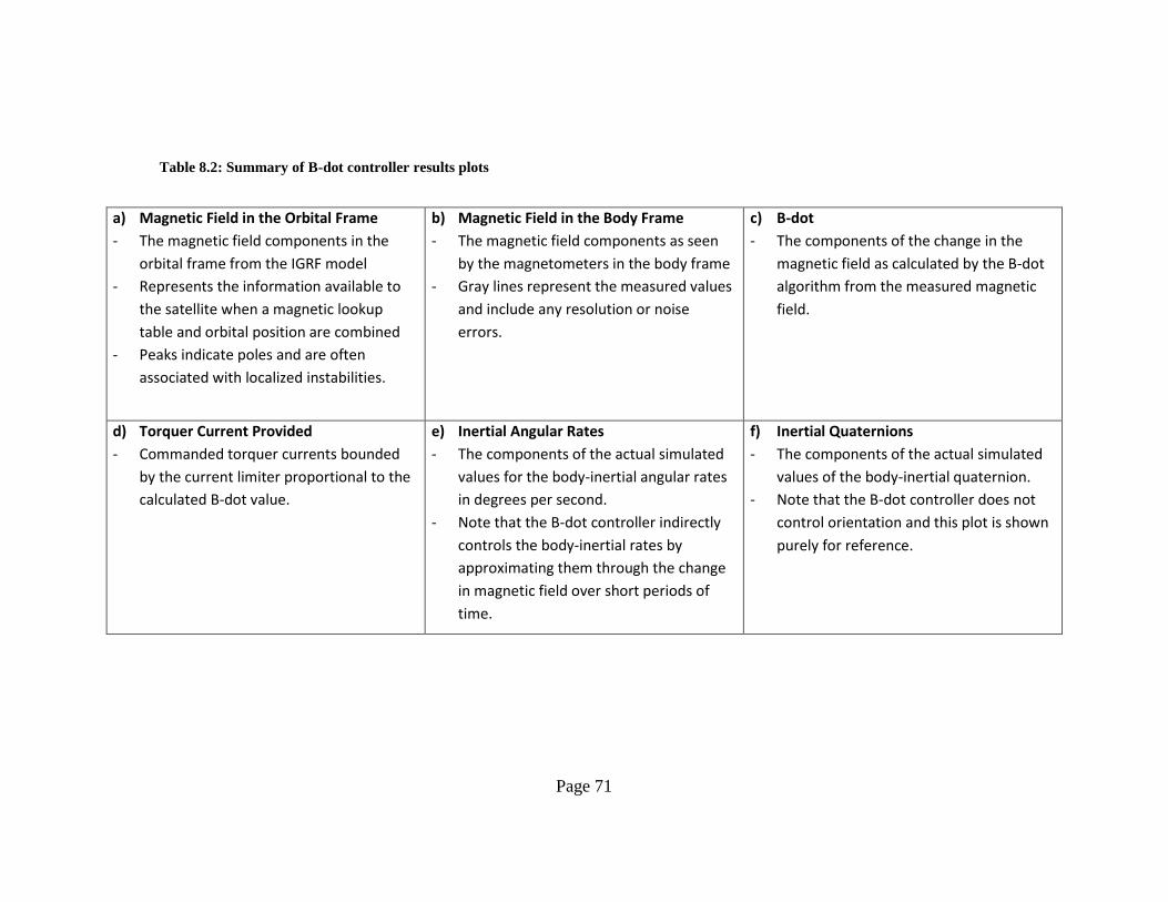
Page 71
Table 8.2: Summary of B-dot controller results plots
a) Magnetic Field in the Orbital Frame
- The magnetic field components in the
orbital frame from the IGRF model
- Represents the information available to
the satellite when a magnetic lookup
table and orbital position are combined
- Peaks indicate poles and are often
associated with localized instabilities.
b) Magnetic Field in the Body Frame
- The magnetic field components as seen
by the magnetometers in the body frame
- Gray lines represent the measured values
and include any resolution or noise
errors.
c) B-dot
- The components of the change in the
magnetic field as calculated by the B-dot
algorithm from the measured magnetic
field.
d) Torquer Current Provided
- Commanded torquer currents bounded
by the current limiter proportional to the
calculated B-dot value.
e) Inertial Angular Rates
- The components of the actual simulated
values for the body-inertial angular rates
in degrees per second.
- Note that the B-dot controller indirectly
controls the body-inertial rates by
approximating them through the change
in magnetic field over short periods of
time.
f) Inertial Quaternions
- The components of the actual simulated
values of the body-inertial quaternion.
- Note that the B-dot controller does not
control orientation and this plot is shown
purely for reference.

Page 72
8.4 Detumbling
Many simulations were run in order to optimize the three main control parameters: gain,
pulse length, and convergence criteria. Upon finding the optimum of each control
parameter, error in the magnetometer readings was included to evaluate the robustness of
the B-dot controller and its performance. For each of the detumbling simulations, a polar
orbit (inclination of 95°) in the middle of ExoCube’s desired altitude range (475 𝑘𝑚)
was selected as a representative test case with large magnetic field variation. The
conservative estimate of the 3U’s stowed moment of inertia that was used in the
simulations is
𝐼𝑡𝑜𝑡𝑎𝑙 = [0.0053 0 0
0 0.0336 00 0 0.0336
]
As mentioned previously, the maximum expected rotation rate imparted by deployment
from the P-POD would be one revolution per minute (Guerrant). Thus the initial rate for
the simulation was set as
𝜔0 = [𝜋 30⁄ 0.05 −0.05] (𝑟𝑎𝑑/𝑠)
Where the maximum rotation is applied about the 𝑏1 axis of the satellite which has the
least magnetorquers and the other terms are perturbation velocities. For simplicity, the
initial orientation was set so that the body frame was aligned with the inertial frame
𝑞0 = [0 0 0 1]

Page 73
8.4.1 Gain Selection
The range of acceptable gains was found by running the simulation with a wide range of
values for 𝐾𝑏𝑑𝑜𝑡. The simulations were run for one and a half orbits which was deemed a
reasonable period for detumbling based off of previous missions. No error was
introduced into the magnetometer readings and the pulse lengths were set to 9.9 seconds
based on previous designs. The angular rate and total current draw for each gain tested
was recorded and shown in Figure 8.2.
Figure 8.2: B-dot performance for selected range of gains
As can be seen in Figure 8.2, the angular rate after 1.5 orbits remains fairly consistent at
an average of 0.1823 deg/s save for the gains lower than 2 × 10⁴ which appear to be
underpowered and didn’t converge within 1.5 orbits. Higher gains show faster initial
settling times at the cost of power as evident by the total current draw shown in the
0
5
10
15
20
25
0
0.1
0.2
0.3
0.4
0.5
0.6
0.7
0.8
0.9
1
1.00E+04 1.00E+05 1.00E+06
Tota
l Ch
arge
Dra
w [
Ah
]
Fin
al A
ngu
lar
Rat
e [d
eg/s
]
Gain
Rate
Charge

Page 74
figure. However, for gains above 3 × 10⁵, the simulations show evidence of local
instabilities that occur when the satellite passes over the poles and although the controller
recovers, this behavior draws unnecessary amounts of current and is thus undesirable.
The acceptable range of gains given the conditions of the simulation is therefore between
2 × 10⁴ and 3 × 10⁵. Simulations exemplifying an optimal case, a sub-optimal case, and
local instabilities are shown in detail in the following sections. The sub-optimal case
illustrates the realistic performance given the uncertainties in the actual satellite.

Page 75
8.4.1.1 Optimal Case
Figure 8.3: Optimal gain performance of the B-dot controller
𝐾𝑏𝑑𝑜𝑡 Pulse Length: 𝑑𝑡 [s] Final Rate: ‖𝜔‖ [deg/s]
𝟔 × 𝟏𝟎𝟒 9.9 0.1742
0 20 40 60 80 100 120 140-5
0
5x 10
-5 a) Magnetic Field in Orbital Frame [T]
time [min]
0 20 40 60 80 100 120 140-8
-6
-4
-2
0
2
4
6x 10
-5 b) Magnetic Field in Body Frame [T]
time [min]
0 20 40 60 80 100 120 140-4
-3
-2
-1
0
1
2
3
4x 10
-6 c) B-dot measured [T/s]
time [min]
0 20 40 60 80 100 120 140-0.8
-0.6
-0.4
-0.2
0
0.2
0.4
0.6
0.8d) Torquer Current Provided [A]
time [min]
0 20 40 60 80 100 120 140-6
-4
-2
0
2
4
6e) Inertial Angular rates [deg/s]
time [min]
0 20 40 60 80 100 120 140-1
-0.5
0
0.5
1f) Inertial Quaternions
time [min]

Page 76
8.4.1.2 Sub-Optimal Case
Figure 8.4: Sub-optimal gain performance of the B-dot controller
𝐾𝑏𝑑𝑜𝑡 Pulse Length: 𝑑𝑡 [s] Final Rate: ‖𝜔‖ [deg/s]
𝟑 × 𝟏𝟎𝟒 9.9 0.1950
0 20 40 60 80 100 120 140-5
0
5x 10
-5 a) Magnetic Field in Orbital Frame [T]
time [min]
0 20 40 60 80 100 120 140-8
-6
-4
-2
0
2
4
6x 10
-5 b) Magnetic Field in Body Frame [T]
time [min]
0 20 40 60 80 100 120 140-4
-3
-2
-1
0
1
2
3
4x 10
-6 c) B-dot measured [T/s]
time [min]
0 20 40 60 80 100 120 140-0.5
0
0.5d) Torquer Current Provided [A]
time [min]
0 20 40 60 80 100 120 140-6
-4
-2
0
2
4
6e) Inertial Angular rates [deg/s]
time [min]
0 20 40 60 80 100 120 140-1
-0.5
0
0.5
1f) Inertial Quaternions
time [min]

Page 77
8.4.1.3 Local Instability
Figure 8.5: Simulation depicting local instabilities of B-dot controller due to improper gain selection
𝐾𝑏𝑑𝑜𝑡 Pulse Length: 𝑑𝑡 [s] Final Rate: ‖𝜔‖ [deg/s]
𝟓 × 𝟏𝟎𝟕 9.9 0.4070
0 20 40 60 80 100 120 140-5
0
5x 10
-5 a) Magnetic Field in Orbital Frame [T]
time [min]
0 20 40 60 80 100 120 140-8
-6
-4
-2
0
2
4
6
8x 10
-5 b) Magnetic Field in Body Frame [T]
time [min]
0 20 40 60 80 100 120 140-4
-2
0
2
4
6x 10
-6 c) B-dot measured [T/s]
time [min]
0 20 40 60 80 100 120 140-3
-2
-1
0
1
2
3d) Torquer Current Provided [A]
time [min]
0 20 40 60 80 100 120 140-6
-4
-2
0
2
4
6e) Inertial Angular rates [deg/s]
time [min]
0 20 40 60 80 100 120 140-1
-0.5
0
0.5
1f) Inertial Quaternions
time [min]
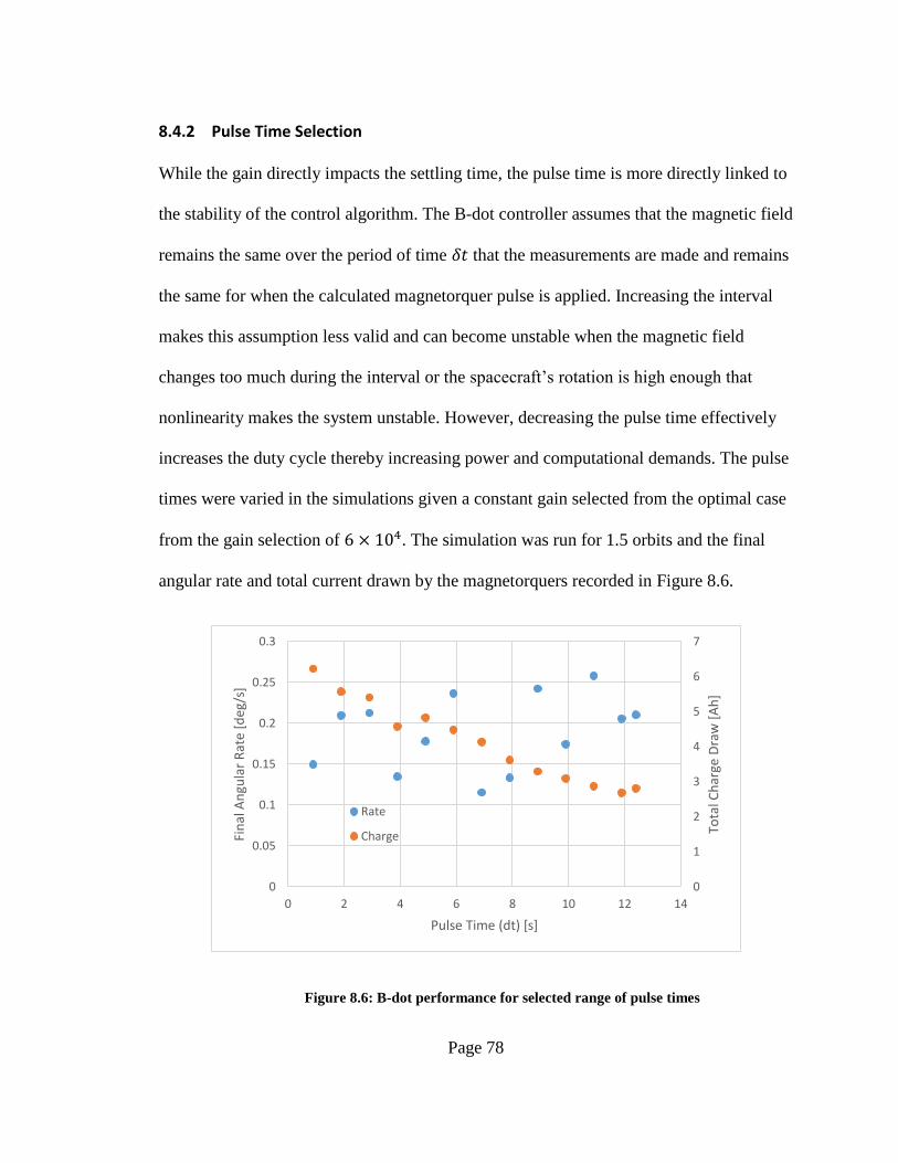
Page 78
8.4.2 Pulse Time Selection
While the gain directly impacts the settling time, the pulse time is more directly linked to
the stability of the control algorithm. The B-dot controller assumes that the magnetic field
remains the same over the period of time 𝛿𝑡 that the measurements are made and remains
the same for when the calculated magnetorquer pulse is applied. Increasing the interval
makes this assumption less valid and can become unstable when the magnetic field
changes too much during the interval or the spacecraft’s rotation is high enough that
nonlinearity makes the system unstable. However, decreasing the pulse time effectively
increases the duty cycle thereby increasing power and computational demands. The pulse
times were varied in the simulations given a constant gain selected from the optimal case
from the gain selection of 6 × 10⁴. The simulation was run for 1.5 orbits and the final
angular rate and total current drawn by the magnetorquers recorded in Figure 8.6.
Figure 8.6: B-dot performance for selected range of pulse times
0
1
2
3
4
5
6
7
0
0.05
0.1
0.15
0.2
0.25
0.3
0 2 4 6 8 10 12 14
Tota
l Ch
arge
Dra
w [
Ah
]
Fin
al A
ngu
lar
Rat
e [d
eg/s
]
Pulse Time (dt) [s]
Rate
Charge

Page 79
As can be seen in Figure 8.6, the rate remains relatively consistent at an average of
0.1740 deg/s for all pulse times until it is increased to 12.5 seconds and the controller
diverges. The figure also shows that the current draw from the magnetorquers increases
as the pulse time is increased. The ideal pulse time thus remains 9.9 seconds as with the
heritage design since it affords a decent margin away from the instability that occurs with
longer pulse times but doesn’t suffer from the increase in current draw. It should be noted
that the ideal pulse time is dependent on the gain and moment of inertia and should be
recalculated given a different scenario. The performance of the ideal pulse time has
already been shown in the previous section since the ideal pulse time remains the same as
the heritage design. Simulation results showing the unstable behavior are shown in the
following section.

Page 80
8.4.2.1 Instability Due to Increased Pulse Time
Figure 8.7: Simulation depicting instability of B-dot controller due to increased pulse time
𝐾𝑏𝑑𝑜𝑡 Pulse Length: 𝑑𝑡 [s] Final Rate: ‖𝜔‖ [deg/s]
6 × 10⁴ 𝟏𝟐. 𝟓 21.3533
0 20 40 60 80 100 120 140-5
0
5x 10
-5 a) Magnetic Field in Orbital Frame [T]
time [min]
0 20 40 60 80 100 120 140-8
-6
-4
-2
0
2
4
6
8x 10
-5 b) Magnetic Field in Body Frame [T]
time [min]
0 20 40 60 80 100 120 140-8
-6
-4
-2
0
2
4
6
8
10x 10
-6 c) B-dot measured [T/s]
time [min]
0 20 40 60 80 100 120 140-1.5
-1
-0.5
0
0.5
1
1.5d) Torquer Current Provided [A]
time [min]
0 20 40 60 80 100 120 140-5
0
5
10
15
20
25e) Inertial Angular rates [deg/s]
time [min]
0 20 40 60 80 100 120 140-1
-0.5
0
0.5
1f) Inertial Quaternions
time [min]
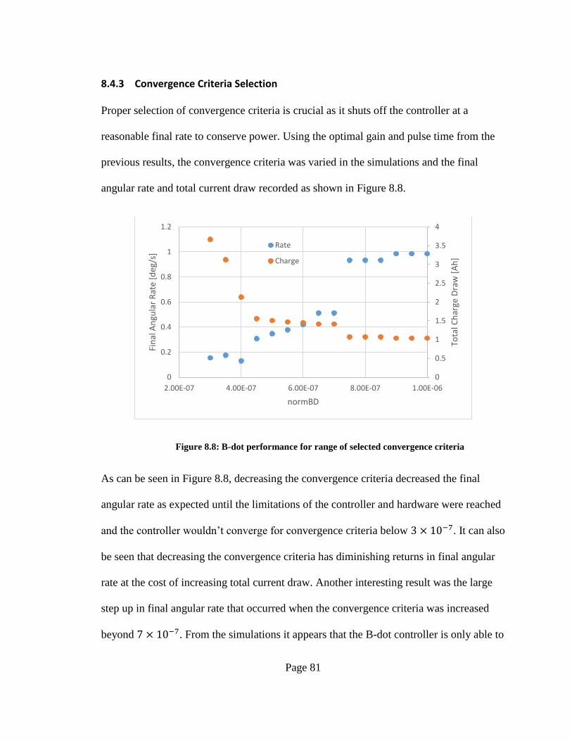
Page 81
8.4.3 Convergence Criteria Selection
Proper selection of convergence criteria is crucial as it shuts off the controller at a
reasonable final rate to conserve power. Using the optimal gain and pulse time from the
previous results, the convergence criteria was varied in the simulations and the final
angular rate and total current draw recorded as shown in Figure 8.8.
Figure 8.8: B-dot performance for range of selected convergence criteria
As can be seen in Figure 8.8, decreasing the convergence criteria decreased the final
angular rate as expected until the limitations of the controller and hardware were reached
and the controller wouldn’t converge for convergence criteria below 3 × 10⁻⁷. It can also
be seen that decreasing the convergence criteria has diminishing returns in final angular
rate at the cost of increasing total current draw. Another interesting result was the large
step up in final angular rate that occurred when the convergence criteria was increased
beyond 7 × 10⁻⁷. From the simulations it appears that the B-dot controller is only able to
0
0.5
1
1.5
2
2.5
3
3.5
4
0
0.2
0.4
0.6
0.8
1
1.2
2.00E-07 4.00E-07 6.00E-07 8.00E-07 1.00E-06
Tota
l Ch
arge
Dra
w [
Ah
]
Fin
al A
ngu
lar
Rat
e [d
eg/s
]
normBD
Rate
Charge

Page 82
perform the initial part of the detumbling with this convergence criteria. Thus the range
of convergence criteria for acceptable performance of the B-dot controller is from 3 ×
10−7 to 7 × 10⁻⁷. The best performance without unnecessary current draw appears to be
for a convergence criteria of 4 × 10⁻⁷.
8.4.4 Minimum Magnetometer Resolution
Given the optimum gain and pulse time, the simulations were run with varying
magnetometer resolution to find the minimum required resolution for convergence. B-dot
was allowed to run for 1.5 orbits and the final angular rates were recorded and can be
seen in Figure 8.9.
Figure 8.9: B-dot performance for range of magnetometer resolutions
As can be seen in Figure 8.9, the final angular rates for the simulations remain consistent
until the resolution of the magnetometers reaches 1 × 10⁻⁵ Teslas, which is the same
0
0.1
0.2
0.3
0.4
0.5
0.6
0.7
0.8
0.9
1
1.00E-07 1.00E-06 1.00E-05 1.00E-04
Fin
al A
ngu
lar
Rat
e [d
eg/s
]
Magnetometer Resolution [T]

Page 83
order of magnitude of the minimum expected Earth magnetic field strength. The impact
of the resolution errors become evident in the step-like behavior of the yaw rates in the
simulation in the next section. If the resolution is decreased to 5 × 10⁻⁵ Teslas, the
controller diverges because it cannot accurate resolve the Earth magnetic field. Thus the
magnetometers should have a resolution on the order of 10−6 Teslas or better.
Simulations showing the impact of the resolution error and divergence are shown in the
following sections.

Page 84
8.4.4.1 Impact of Resolution Error
Figure 8.10: Simulation depicting the impact of magnetometer resolution error on the B-dot controller
𝐾𝑏𝑑𝑜𝑡 Pulse Length:
𝑑𝑡 [s]
Magnetometer
Noise: 𝜎𝐵 [T]
Magnetometer
Resolution [T]
Final Rate:
‖𝜔‖ [deg/s]
6 × 10⁴ 9.9 0 𝟐 × 𝟏𝟎−𝟓 0.2070
0 20 40 60 80 100 120 140-5
0
5x 10
-5 a) Magnetic Field in Orbital Frame [T]
time [min]
0 20 40 60 80 100 120 140-8
-6
-4
-2
0
2
4
6
8x 10
-5 b) Magnetic Field in Body Frame [T]
time [min]
0 20 40 60 80 100 120 140-3
-2
-1
0
1
2
3
4
5x 10
-6 c) B-dot measured [T/s]
time [min]
0 20 40 60 80 100 120 140-1.2
-1
-0.8
-0.6
-0.4
-0.2
0
0.2
0.4
0.6d) Torquer Current Provided [A]
time [min]
0 20 40 60 80 100 120 140-6
-4
-2
0
2
4
6e) Inertial Angular rates [deg/s]
time [min]
0 20 40 60 80 100 120 140-1
-0.5
0
0.5
1f) Inertial Quaternions
time [min]
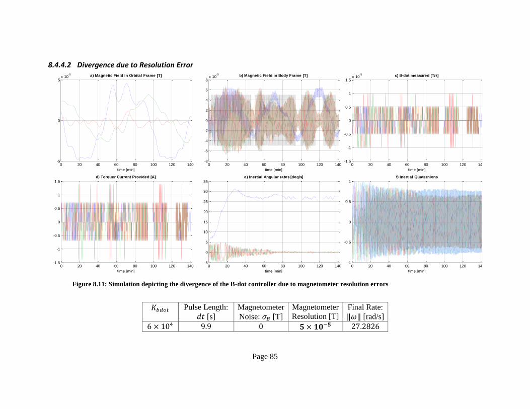
Page 85
8.4.4.2 Divergence due to Resolution Error
Figure 8.11: Simulation depicting the divergence of the B-dot controller due to magnetometer resolution errors
𝐾𝑏𝑑𝑜𝑡 Pulse Length:
𝑑𝑡 [s]
Magnetometer
Noise: 𝜎𝐵 [T]
Magnetometer
Resolution [T]
Final Rate:
‖𝜔‖ [rad/s]
6 × 10⁴ 9.9 0 𝟓 × 𝟏𝟎−𝟓 27.2826
0 20 40 60 80 100 120 140-5
0
5x 10
-5 a) Magnetic Field in Orbital Frame [T]
time [min]
0 20 40 60 80 100 120 140-8
-6
-4
-2
0
2
4
6
8x 10
-5 b) Magnetic Field in Body Frame [T]
time [min]
0 20 40 60 80 100 120 140-1.5
-1
-0.5
0
0.5
1
1.5x 10
-5 c) B-dot measured [T/s]
time [min]
0 20 40 60 80 100 120 140-1.5
-1
-0.5
0
0.5
1
1.5d) Torquer Current Provided [A]
time [min]
0 20 40 60 80 100 120 140-5
0
5
10
15
20
25
30
35e) Inertial Angular rates [deg/s]
time [min]
0 20 40 60 80 100 120 140-1
-0.5
0
0.5
1f) Inertial Quaternions
time [min]

Page 86
8.4.5 Magnetometer Noise Tolerance
Given the optimum gain and pulse time, the simulations were run with a magnetometer
resolution of 1 × 10⁻⁵ Tesla and the standard deviation of the magnetometer noise varied
to find the maximum allowable noise for convergence. B-dot was allowed to run for 1.5
orbits and the final angular rates were recorded and can be seen in Figure 8.12.
Figure 8.12: B-dot performance for range of magnetometer noise levels
As can be seen in Figure 8.12, the angular rate remains consistent until the magnetometer
noise has a standard deviation around 3 × 10⁻⁶, about an order of magnitude less than
the minimum magnetic field strength. The final angular rates of the simulation increase to
over 1 deg/s as the standard deviation of the noise is increased to 3 × 10⁻⁵, the same
magnitude as the Earth magnetic field, after which the controller diverges.
0
0.2
0.4
0.6
0.8
1
1.2
1.4
1.6
1.00E-07 1.00E-06 1.00E-05 1.00E-04
Fin
al A
ngu
lar
Rat
e [d
eg/s
]
Magnetometer Noise (σ)

Page 87
8.5 Guide to PD Controller Results Plots
In the following sections, several key simulations have been selected from the many run
to demonstrate various aspects of the performance of the PD controller. The results of
each simulation are summarized in a single figure containing six subplots a-f which are
detailed in Table 8.3. The x-axis of all subplots are given in minutes. The line of each
subplot except for the quaternions are colored accordingly as
𝑋𝐵𝑜𝑑𝑦: 𝐵𝑙𝑢𝑒 𝑌𝐵𝑜𝑑𝑦: 𝐺𝑟𝑒𝑒𝑛 𝑍𝐵𝑜𝑑𝑦: 𝑅𝑒𝑑
For the quaternion plots the vector components are represented by the above colors and
approximate the body orientation when close to alignment with the reference frame. The
scalar component of the quaternion is represented by the cyan colored line.
The line types also represent different information as follows:
Solid: Actual values used by the simulation representing the most accurate information
available.
Dashed: Desired values used by the control algorithm
Gray: Measured values used by the control algorithm that include resolution and noise
errors.

Page 88
Table 8.3: Summary of PD controller results plots
a) Quaternion Error
- Shows the quaternion relating the actual
and desired orientation of the satellite.
- The vector components of the error
quaternion are used to calculate the
control torque
- Gray lines represent the error quaternion
calculated using the measured body-
inertial quaternion and includes any
resolution or noise errors
b) Inertial Angular Rates
- The components of the actual simulated
values of the body-inertial rates
- The dotted lines represent the desired
inertial rates
- Gray lines represent the measured values
and include any resolution or noise errors
- The difference between the measured
body-inertial and desired rates is used in
the control law
c) Inertial Quaternions
- The components of the actual simulated
values of the body-inertial quaternion
- The dotted lines represent the desired
inertial quaternion
- Gray lines represent the measured values
and include any resolution or noise errors
- The measured and desired quaternions
are used to calculate the quaternion error
in subplot a.
d) Pointing Error
- Represents the error rotation angle about
the quaternion error axis.
- Calculated from the scalar component of
the error quaternion as follows:
𝜃𝑒𝑟𝑟 = 2 acos(𝑞4,𝑒𝑟𝑟)
e) Orbital Angular Rates
- The components of the actual simulated
values of the body-orbital rates
- The dotted lines represent the desired
orbital rates
- This plot is included as reference and is
not used in the calculation of the control
torques
f) Orbital Quaternions
- The components of the actual simulated
values of the body-orbital quaternion
- The dotted lines represent the desired
orbital quaternion
- This plot is included as reference and is
not used in the calculation of the control
torques.

Page 89
8.6 Initial Attitude Acquisition
After successfully detumbling, the spacecraft will have relatively low angular rates that
can be conservatively approximated as:
𝜔0 = [0.005 − 0.005 0.002]
Although B-dot will reduce the angular rates of the spacecraft, the orientation will be
unknown and possibly at a large angle from the desired ram pointing orientation. For a
robust test of the PD controller’s performance, the initial orientation is set to 120 degrees
off of the target orientation as given by the quaternion
𝑞0 = [0.5 0.5 0.5 0.5]
As with the detumbling simulations, a polar orbit with an inclination of 95 degrees at an
altitude of 475 km was selected for the simulation. A conservative estimate of the 3U's
deployed moment of inertia that was used in the simulation is
𝐼𝑡𝑜𝑡𝑎𝑙 = [0.0049 0 0
0 0.1236 00 0 0.1238
]
The given deployed moment of inertia is gravity gradient stable per the smelt parameters
defined previously as indicated by the red x in the Lagrange stability region seen in
Figure 8.13.

Page 90
Figure 8.13: Smelt parameter plane with deployed configuration plotted (indicated by red X)
8.6.1 Gain Selection
As discussed previously, Wie et al. shows that global stability for the quaternion
feedback regulator is guaranteed provided that the rate gain is scaled by the spacecraft
moments of inertia (Wie, Weiss and Arapostathis). When the control torques are applied
directly as if the system had three reaction wheels, the controller responds well for a wide
range of gains scaled by the moment of inertia. However, when direct actuation is
replaced by the use of magnetorquers, the yaw motion exhibits local instabilities for the
wide range of gains tested. This makes sense given that the gain design technique
outlined by Wie et al. is based on a second order linear differential equation and active

Page 91
magnetic control is inherently non-linear due to the inability to actuate in all 3 axes at all
times.
By eliminating the scaling by the moment of inertia for the rate gain, the yaw instabilities
were reduced but the system still didn't converge. Next the gyroscopic cancelation
component was removed and the yaw instability issues improved and the system
converged for a narrow range of gains. Upon applying the current limiters that are a
necessity of the magnetorquer hardware, the range of gains that converge narrows further.
The current limiters essentially requires lower gain values in order to avoid the instability
that comes with clipping the control torques.
Ultimately, a line search method was adopted to find the optimum gains. First a battery of
equal rate and orientation gains were simulated that were scaled so that the rate gain was
three orders of magnitude higher than the orientation gain. Given the results of the first
battery of tests, the pair of gains with the fastest convergence time was selected and the
rate gain varied while the orientation gain was held constant. Given the results of the
second battery of tests, the pair of gains with the fastest convergence time was selected
and then the orientation gain was varied while the rate gain was held constant. This
procedure was repeated until minimal improvement was seen thus suggesting an optimal
set of gains have been found. The data from this line search can be found in appendix B
and the results from the optimal set of gains seen in the following section. Also included
is a simulation with a sub-optimal set of gains to show the corresponding losses in
performance.

Page 92
8.6.1.1 Optimal Case
Figure 8.14: Optimal gain performance of PD controller for initial acquisition of the target orientation
𝐷𝑃𝐷 𝐾𝑃𝐷 Convergence Criteria:
𝜔𝑡𝑜𝑙 [deg/s], ∠𝑡𝑜𝑙 [deg]
Time to Converge
[min] Rate: ‖𝜔‖ [deg/s] Pointing Error
[deg]
8 × 10⁻⁴ 5 × 10⁻⁶ 1 × 10⁻³, 2 197.165 5.74 × 10⁻⁴ 1.1883
0 50 100 150 200 250 300 350 400 450-1
-0.5
0
0.5
1a) Error Quaternion
time [min]
0 50 100 150 200 250 300 350 400 450-0.4
-0.2
0
0.2
0.4
0.6
0.8
1b) Inertial Angular Rates [deg/s]
time [min]
0 50 100 150 200 250 300 350 400 450-1
-0.5
0
0.5
1c) Inertial Quaternions
time [min]
0 50 100 150 200 250 300 350 400 4500
10
20
30
40
50
60d) Pointing Error [deg]
time [min]
0 50 100 150 200 250 300 350 400 450-0.5
0
0.5
1e) Orbital Angular Rates [deg/s]
time [min]
0 50 100 150 200 250 300 350 400 450-1
-0.5
0
0.5
1f) Orbital Quaternions
time [min]

Page 93
8.6.1.2 Sub-Optimal Case
Figure 8.15: Sub-optimal gain performance of PD controller for initial acquisition of the target orientation
𝐷𝑃𝐷 𝐾𝑃𝐷 Convergence Criteria:
𝜔𝑡𝑜𝑙 [deg/s], ∠𝑡𝑜𝑙 [deg]
Time to Converge
[min] Rate: ‖𝜔‖ [deg/s] Pointing Error
[deg]
1 × 10⁻³ 1 × 10⁻⁶ 1 × 10⁻³, 2 450.165 9.45 × 10⁻⁴ 1.8455
0 100 200 300 400 500 600 700 800 900-1
-0.5
0
0.5
1a) Error Quaternion
time [min]
0 100 200 300 400 500 600 700 800 900-0.4
-0.3
-0.2
-0.1
0
0.1
0.2
0.3
0.4b) Inertial Angular Rates [deg/s]
time [min]
0 100 200 300 400 500 600 700 800 900-1
-0.5
0
0.5
1c) Inertial Quaternions
time [min]
0 100 200 300 400 500 600 700 800 9000
10
20
30
40
50
60d) Pointing Error [deg]
time [min]
0 100 200 300 400 500 600 700 800 900-0.4
-0.3
-0.2
-0.1
0
0.1
0.2
0.3
0.4e) Orbital Angular Rates [deg/s]
time [min]
0 100 200 300 400 500 600 700 800 900-1
-0.5
0
0.5
1f) Orbital Quaternions
time [min]

Page 94
8.6.2 Pulse Time Selection
To determine the impact of pulse time on the performance of the three axis controller, the
optimal gains selected from the previous section were used while the pulse time was
varied. The time to converge and charge used remained relatively constant at an average
of 300 minutes and 1.33 Amp-hours for a large range of pulse times as can be seen in
Figure 8.16
Figure 8.16: PD controller performance for range of pulse times
Once the pulse times were increased to13.9 seconds and greater, localized instability was
observed coinciding with passing over the magnetic poles. As with the B-dot controller,
increased pulse times cause the performance of the controller to suffer near the poles due
to the fact that the magnetic field vector that the pulse was calculated for changes too
much during the pulse. Decreased pulse times lead to increases in computational
0
5
10
15
20
25
0
100
200
300
400
500
600
700
800
0 5 10 15 20
Tota
l Ch
arge
Dra
w [
Ah
]
Tim
e to
Co
nve
rge
[min
]
Pulse Time (dt) [s]
Time to Converge
Charge

Page 95
demands and must be balanced with the stability of the controller. In order maintain a
comfortable margin from the instabilities observed with increased pulse time without
overtaxing the flight computer, a pulse time of 9.9 seconds was selected and is consistent
with the B-dot controller design.
8.6.3 Convergence Criteria
Selection of the convergence criteria for the PD controller directly impacts the final
pointing accuracy of the spacecraft. The offset in spacecraft orientation from the target
orientation and the angular rate at convergence will determine the offset and oscillation
of the spacecraft once the momentum wheel has been brought to the desired speed. The
impact of the offset in pointing was found to have far less of an impact than the angular
rates and thus the convergence criteria for offset was conservatively set at 2 degrees. The
following figure shows the behavior of the satellite in the target orientation given
different angular rates without the influence of aerodynamic and solar radiation pressure
torques.

Page 96
Figure 8.17: Spacecraft pointing error for various initial angular rates
As can be seen in Figure 8.17, angular rates above 0.003 deg/s cause the satellite to
oscillate outside of the required ten degree pointing. In order to ensure that the
momentum wheel spins up in an acceptable orientation and that the spacecraft will
remain in the target orientation barring a large offset in the center of gravity, a
convergence criteria of 0.001 deg/s was set.
8.6.4 Orientation Error Tolerance
Given the optimal gains and pulse time, the simulations were run while varying the
resolution of the attitude quaternion to find the minimum required resolution for
convergence. Since the vector portion of the quaternion error approaches zero as the
0 100 200 300 400 500 600 700 800 900 10000
5
10
15Pointing Error [deg]
time [min]
0 = 0.001 deg/s
0 = 0.002 deg/s
0 = 0.003 deg/s
0 = 0.004 deg/s

Page 97
controller converges, the impact of the rounding errors isn’t seen until after the controller
has already brought the spacecraft close to the target orientation. As a result, the
controller will converge with a minimum resolution of 1 × 10⁻¹ as can be seen in the
next section. However, the attitude knowledge errors exceed 40 degrees which is outside
of the required ± 5 degree pointing knowledge requirement required by the payload.
Having a resolution of at least 1 × 10⁻⁵ guaranteed no impact on the performance of the
controller.
Given a resolution of 1 × 10⁻⁵, noise was introduced into the attitude quaternions with
varying standard deviations to find the maximum allowable amount of noise for
convergence. As with the resolution, the noise primarily effects the performance of the
controller after it gets close to the target orientation. It was found that the controller still
converged with attitude quaternion noise with a standard deviation of 5 × 10⁻² as can be
seen in the following section. However, this noise represented errors in pointing
knowledge as high as 60 degrees and is thus unacceptable per the payload pointing
knowledge requirements. It is recommended that the noise not exceed the resolution of
1 × 10⁻⁵ in order to avoid an impact on controller performance.

Page 98
8.6.4.1 Minimum Resolution
Figure 8.18: Simulation depicting the impact of quaternion resolution on the PD controller
𝐷𝑃𝐷 𝐾𝑃𝐷 Convergence Criteria:
𝜔𝑡𝑜𝑙 [deg/s], ∠𝑡𝑜𝑙 [deg]
Time to Converge
[min] Rate: ‖𝜔‖ [deg/s] Pointing Error
[deg]
8 × 10⁻⁴ 5 × 10⁻⁶ 1 × 10⁻³, 2 582.4983 6.7008 × 10⁻⁴ 0.5558
0 100 200 300 400 500 600 700 800 900-1
-0.5
0
0.5
1a) Error Quaternion
time [min]
0 100 200 300 400 500 600 700 800 900-0.5
0
0.5
1b) Inertial Angular Rates [deg/s]
time [min]
0 100 200 300 400 500 600 700 800 900-1
-0.5
0
0.5
1c) Inertial Quaternions
time [min]
0 100 200 300 400 500 600 700 800 9000
10
20
30
40
50
60d) Pointing Error [deg]
time [min]
0 100 200 300 400 500 600 700 800 900-0.5
0
0.5
1e) Orbital Angular Rates [deg/s]
time [min]
0 100 200 300 400 500 600 700 800 900-1
-0.5
0
0.5
1f) Orbital Quaternions
time [min]
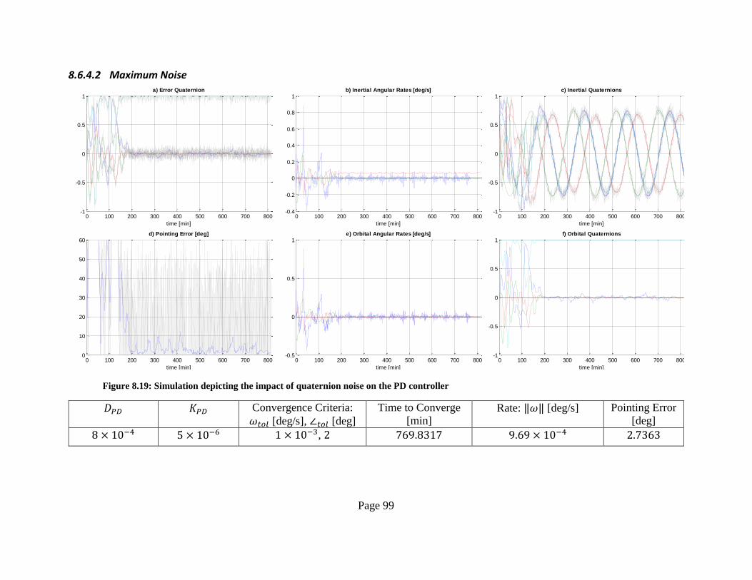
Page 99
8.6.4.2 Maximum Noise
Figure 8.19: Simulation depicting the impact of quaternion noise on the PD controller
𝐷𝑃𝐷 𝐾𝑃𝐷 Convergence Criteria:
𝜔𝑡𝑜𝑙 [deg/s], ∠𝑡𝑜𝑙 [deg]
Time to Converge
[min] Rate: ‖𝜔‖ [deg/s] Pointing Error
[deg]
8 × 10⁻⁴ 5 × 10⁻⁶ 1 × 10⁻³, 2 769.8317 9.69 × 10⁻⁴ 2.7363
0 100 200 300 400 500 600 700 800-1
-0.5
0
0.5
1a) Error Quaternion
time [min]
0 100 200 300 400 500 600 700 800-0.4
-0.2
0
0.2
0.4
0.6
0.8
1b) Inertial Angular Rates [deg/s]
time [min]
0 100 200 300 400 500 600 700 800-1
-0.5
0
0.5
1c) Inertial Quaternions
time [min]
0 100 200 300 400 500 600 700 8000
10
20
30
40
50
60d) Pointing Error [deg]
time [min]
0 100 200 300 400 500 600 700 800-0.5
0
0.5
1e) Orbital Angular Rates [deg/s]
time [min]
0 100 200 300 400 500 600 700 800-1
-0.5
0
0.5
1f) Orbital Quaternions
time [min]
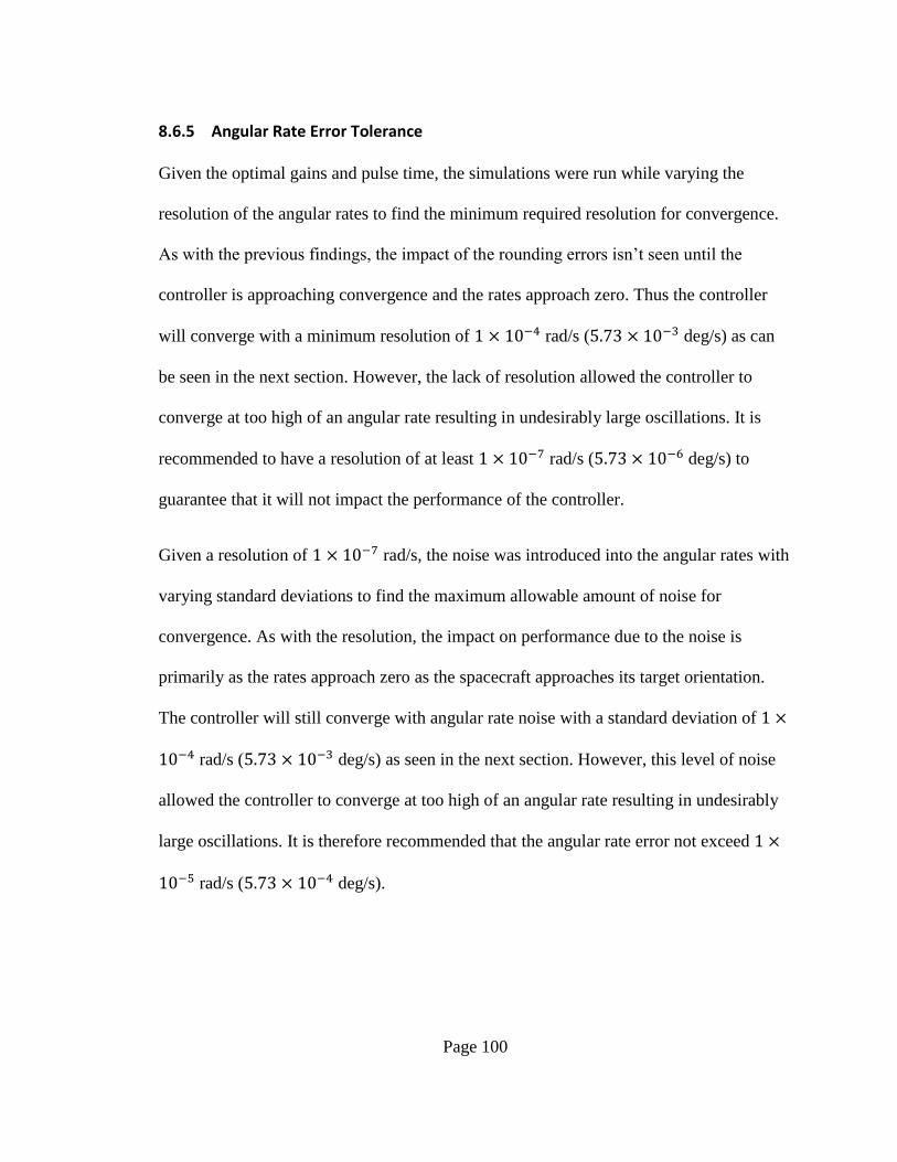
Page 100
8.6.5 Angular Rate Error Tolerance
Given the optimal gains and pulse time, the simulations were run while varying the
resolution of the angular rates to find the minimum required resolution for convergence.
As with the previous findings, the impact of the rounding errors isn’t seen until the
controller is approaching convergence and the rates approach zero. Thus the controller
will converge with a minimum resolution of 1 × 10⁻⁴ rad/s (5.73 × 10⁻³ deg/s) as can
be seen in the next section. However, the lack of resolution allowed the controller to
converge at too high of an angular rate resulting in undesirably large oscillations. It is
recommended to have a resolution of at least 1 × 10⁻⁷ rad/s (5.73 × 10⁻⁶ deg/s) to
guarantee that it will not impact the performance of the controller.
Given a resolution of 1 × 10⁻⁷ rad/s, the noise was introduced into the angular rates with
varying standard deviations to find the maximum allowable amount of noise for
convergence. As with the resolution, the impact on performance due to the noise is
primarily as the rates approach zero as the spacecraft approaches its target orientation.
The controller will still converge with angular rate noise with a standard deviation of 1 ×
10−4 rad/s (5.73 × 10⁻³ deg/s) as seen in the next section. However, this level of noise
allowed the controller to converge at too high of an angular rate resulting in undesirably
large oscillations. It is therefore recommended that the angular rate error not exceed 1 ×
10−5 rad/s (5.73 × 10⁻⁴ deg/s).

Page 101
8.6.5.1 Minimum Resolution
Figure 8.20: Simulation depicting the impact of rate resolution on the PD controller
𝐷𝑃𝐷 𝐾𝑃𝐷 Convergence Criteria:
𝜔𝑡𝑜𝑙 [deg/s], ∠𝑡𝑜𝑙 [deg]
Time to Converge
[min] Rate: ‖𝜔‖ [deg/s] Pointing Error
[deg]
8 × 10⁻⁴ 5 × 10⁻⁶ 1 × 10⁻³, 2 159.8317 0.0039 1.8298
0 100 200 300 400 500 600 700 800 900-1
-0.5
0
0.5
1a) Error Quaternion
time [min]
0 100 200 300 400 500 600 700 800 900-0.5
0
0.5
1b) Inertial Angular Rates [deg/s]
time [min]
0 100 200 300 400 500 600 700 800 900-1
-0.5
0
0.5
1c) Inertial Quaternions
time [min]
0 100 200 300 400 500 600 700 800 9000
10
20
30
40
50
60d) Pointing Error [deg]
time [min]
0 100 200 300 400 500 600 700 800 900-0.5
0
0.5
1e) Orbital Angular Rates [deg/s]
time [min]
0 100 200 300 400 500 600 700 800 900-1
-0.5
0
0.5
1f) Orbital Quaternions
time [min]
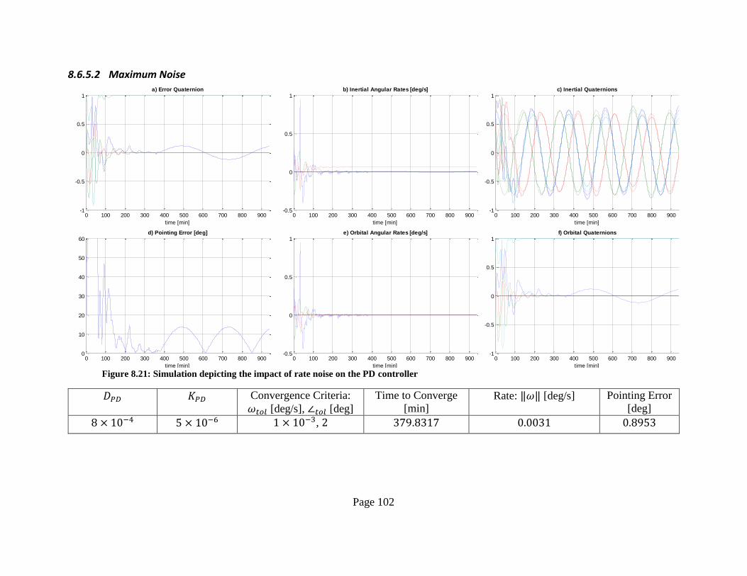
Page 102
8.6.5.2 Maximum Noise
Figure 8.21: Simulation depicting the impact of rate noise on the PD controller
𝐷𝑃𝐷 𝐾𝑃𝐷 Convergence Criteria:
𝜔𝑡𝑜𝑙 [deg/s], ∠𝑡𝑜𝑙 [deg]
Time to Converge
[min] Rate: ‖𝜔‖ [deg/s] Pointing Error
[deg]
8 × 10⁻⁴ 5 × 10⁻⁶ 1 × 10⁻³, 2 379.8317 0.0031 0.8953
0 100 200 300 400 500 600 700 800 900-1
-0.5
0
0.5
1a) Error Quaternion
time [min]
0 100 200 300 400 500 600 700 800 900-0.5
0
0.5
1b) Inertial Angular Rates [deg/s]
time [min]
0 100 200 300 400 500 600 700 800 900-1
-0.5
0
0.5
1c) Inertial Quaternions
time [min]
0 100 200 300 400 500 600 700 800 9000
10
20
30
40
50
60d) Pointing Error [deg]
time [min]
0 100 200 300 400 500 600 700 800 900-0.5
0
0.5
1e) Orbital Angular Rates [deg/s]
time [min]
0 100 200 300 400 500 600 700 800 900-1
-0.5
0
0.5
1f) Orbital Quaternions
time [min]
Page 103
8.7 Wheel Spin Up
After successfully acquiring the target ram-pointing orientation, the spacecraft’s
orientation and angular rates can be conservatively set as
𝜔0 = [−1.9685 × 10⁻⁶ − 1.7453 × 10⁻⁵ 0.0011]
𝑞0 = [0.7372 − 5.3829 × 10⁻⁴ 0.0123 0.6756]
Which corresponds to pointing errors of 1 degree in the pitch and yaw axes and body-
orbital angular rates of 0.001 deg/s which are consistent with the convergence criteria
established previously. The simulations were run for ten orbits with the wheel initially
spinning up with the PD controller on and the convergence check off until the wheel was
at speed and the controller allowed to correct any offset in pointing created during spin
up. Initial simulations led to several key adjustments to the controller and the definition
of the constant torque at which the wheel would be commanded to track until it reached
the desired speed.
From the initial battery of simulations, it was discovered that including the gyroscopic
cancelation component of controller was detrimental to performance and created
instabilities due to the changes in wheel speed. It was also found that the gyroscopic
cancelation component overpowered the relatively small control torques required for the
fine adjustments after the wheel was at speed. Thus the gyroscopic cancelation
component was omitted from the controller after the initial acquisition. It was also
discovered that the optimal gains from the initial acquisition needed to be adjusted by
having the rate gain reduced from 8 × 10⁻⁴ to 5 × 10⁻⁴ in order to avoid the controller

Page 104
overreacting to changes in the rate error when the spacecraft is already within the desired
orientation. The next design task was to set the desired angular speed of the momentum
wheel and the constant torque at which it would be brought to this desired speed.
The Sinclair wheel selected is capable of spinning at a maximum of 3410 rpm resulting in
a momentum storage of 10 mNm/s drawing 0.16 W at steady state (Sinclair Data sheet).
As a compromise between momentum storage and power consumption, a nominal
angular rate of 2000 rpm was selected achieving 5.9 mNm/s momentum storage at a
steady state power consumption of just 0.1 W. As mentioned previously, the momentum
wheel will be commanded to track a constant torque target during spin up until the
desired angular speed is reached. Spin up of the wheel will inevitably cause a temporary
offset in pointing in the pitch axis as a result of a constant torque being applied in one
direction and being opposed by the gravity gradient torques and magnetorquers. The
constant torque in the spacecraft pitch axis was selected to be low enough to be opposed
primarily by the gravity gradient torques and produce an offset that remained within the
pointing requirement of ± 10 degrees. By commanding the wheel to spin up by tracking
a constant torque of 2 × 10⁻⁷ Nm, the spacecraft maintained a 7 degree offset in pointing
on the pitch axis and quickly reacquires the desired orientation once the wheel reached
2000 rpm as can be seen in the following section. As mentioned previously, the torque
control on the wheel has noise on the order of 10−6 Nm associated with it. Despite the
noise level being greater than the commanded torque, the controller can still track the
commanded torque. The spacecraft still remains within 10 degrees of the ram direction

Page 105
but noise in the torque controller causes the offset angle during spin up to vary between 3
and 9 degrees as can be seen in the next section.
Page 106
8.7.1 Wheel Spin Up Performance
Figure 8.22: PD controller performance during wheel spin up
𝐷𝑃𝐷 𝐾𝑃𝐷 Final Wheel
Speed [RPM]
Spin Up
Torque [Nm]
Convergence Criteria:
𝜔𝑡𝑜𝑙 [deg/s], ∠𝑡𝑜𝑙 [deg]
Time to
Converge [min] Rate: ‖𝜔‖
[deg/s]
Pointing
Error [deg]
5 × 10⁻⁴ 5 × 10⁻⁶ 2000 2 × 10⁻⁷ 1 × 10⁻³ 518.165 5.45 × 10⁻⁴ 1.792
0 100 200 300 400 500 600 700 800 900-1
-0.5
0
0.5
1a) Error Quaternion
time [min]
0 100 200 300 400 500 600 700 800 900-0.1
-0.05
0
0.05
0.1b) Inertial Angular Rates [deg/s]
time [min]
0 100 200 300 400 500 600 700 800 900-1
-0.5
0
0.5
1c) Inertial Quaternions
time [min]
0 100 200 300 400 500 600 700 800 9000
10
20
30
40
50
60d) Pointing Error [deg]
time [min]
0 100 200 300 400 500 600 700 800 900-0.06
-0.04
-0.02
0
0.02
0.04
0.06e) Orbital Angular Rates [deg/s]
time [min]
0 100 200 300 400 500 600 700 800 900-1
-0.5
0
0.5
1f) Orbital Quaternions
time [min]

Page 107
8.7.2 Wheel Spin Up Performance with Torque Control Noise
Figure 8.23: PD controller performance during wheel spin up with noise in torque control (𝝈 = 𝟏 × 𝟏𝟎−𝟔)
𝐷𝑃𝐷 𝐾𝑃𝐷 Final Wheel
Speed [RPM]
Spin Up
Torque [Nm]
Convergence Criteria:
𝜔𝑡𝑜𝑙 [deg/s], ∠𝑡𝑜𝑙 [deg]
Time to
Converge [min] Rate: ‖𝜔‖
[deg/s]
Pointing
Error [deg]
5 × 10⁻⁴ 5 × 10⁻⁶ 2000 2 × 10⁻⁷ 1 × 10⁻³ 531.8317 5.37 × 10⁻⁴ 1.3122
0 100 200 300 400 500 600 700 800 900-1
-0.5
0
0.5
1a) Error Quaternion
time [min]
0 100 200 300 400 500 600 700 800 900-0.2
-0.15
-0.1
-0.05
0
0.05
0.1
0.15b) Inertial Angular Rates [deg/s]
time [min]
0 100 200 300 400 500 600 700 800 900-1
-0.5
0
0.5
1c) Inertial Quaternions
time [min]
0 100 200 300 400 500 600 700 800 9000
10
20
30
40
50
60d) Pointing Error [deg]
time [min]
0 100 200 300 400 500 600 700 800 900-0.1
-0.05
0
0.05
0.1e) Orbital Angular Rates [deg/s]
time [min]
0 100 200 300 400 500 600 700 800 900-1
-0.5
0
0.5
1f) Orbital Quaternions
time [min]
Page 108
8.8 Attitude Maintenance
In the event that the spacecraft drifts from its target orientation during wheel spin up or
the spacecraft loses pointing, the attitude control system must reacquire the target
orientation. This is not a trivial task as the momentum wheel adds gyroscopic stiffness in
the already coupled roll and yaw dynamics. With the added challenge of the non-linearity
of magnetic actuation, reacquisition is not feasible with the momentum wheel running.
The required procedure for reacquisition is thus as follows:
The momentum wheel is despun slowly at a constant torque while opposed by the
magnetorquers via the active magnetic control routine
Once the momentum wheel has been brought to rest the active magnetic control
routine will reacquire the target orientation
Upon successful reacquisition of the target orientation the momentum wheel will be
commanded to spin up back to the desired speed at a constant torque while opposed by
the magnetorquers
This procedure was simulated with initial angular rates the same as the initial wheel spin
up as
𝜔0 = [−1.9685 × 10⁻⁶ − 1.7453 × 10⁻⁵ 0.0011]
The initial orientation however was set to represent an 11 degree offset in the yaw and
pitch axes
𝑞0 = [0.7243 − 0.0059 0.1348 0.6762]
The simulation was run for 15 orbits with the wheel initially set to spin down with the PD
controller active and the convergence check off until the wheel was off. The controller
was then allowed to reacquire the ram pointing orientation per the convergence criteria

Page 109
established previously and the wheel set to spin up following the same procedure as the
initial spin up. As can be seen in the following section, the spacecraft loses pointing as
the wheel is spun down but promptly reacquires the target orientation and performs in a
similar fashion to the previous section. The noise from the wheel torque controller was
included for a more realistic simulation.

Page 110
8.8.1 Reacquisition
Figure 8.24: PD controller performance for reacquisition of pointing with torque control noise (𝝈 = 𝟏 × 𝟏𝟎−𝟔)
𝐷𝑃𝐷 𝐾𝑃𝐷 Final Wheel
Speed [RPM]
Spin Up
Torque [Nm]
Convergence Criteria:
𝜔𝑡𝑜𝑙 [deg/s], ∠𝑡𝑜𝑙 [deg]
Time to
Converge [min] Rate: ‖𝜔‖
[deg/s]
Pointing
Error [deg]
5 × 10⁻⁴ 5 × 10⁻⁶ 2000 2 × 10⁻⁷ 1 × 10⁻³ 1341.8 9.00 × 10⁻⁴ 1.9978
0 200 400 600 800 1000 1200 1400-1
-0.5
0
0.5
1a) Error Quaternion
time [min]
0 200 400 600 800 1000 1200 1400-3
-2
-1
0
1
2
3b) Inertial Angular Rates [deg/s]
time [min]
0 200 400 600 800 1000 1200 1400-1
-0.5
0
0.5
1c) Inertial Quaternions
time [min]
0 200 400 600 800 1000 1200 14000
10
20
30
40
50
60d) Pointing Error [deg]
time [min]
0 200 400 600 800 1000 1200 1400-2
-1.5
-1
-0.5
0
0.5
1
1.5
2e) Orbital Angular Rates [deg/s]
time [min]
0 200 400 600 800 1000 1200 1400-1
-0.5
0
0.5
1f) Orbital Quaternions
time [min]

Page 111
9 Conclusions
A combination of a gravity gradient system with a momentum bias wheel was proposed
to meet pointing requirements while reducing power requirements and overall system
complexity. A MATLAB simulation of dynamic and kinematic behavior of the system in
orbit was implemented to guide system design and verify that the pointing requirements
will be met. The problem was broken into four phases: detumbling, initial attitude
acquisition, wheel spin-up, and attitude maintenance.
For the initial phase of detumbling, the B-dot controller has been shown to be a simple
but thoroughly robust method. The results show that it is stable for a wide range of gains
and pulse times. The controller is directly limited by the approximation of the body
angular rates using the change in the magnetic field. This limitation is most evident when
the pulse time is too long, magnetometer resolution too low, or magnetometer noise too
high. The final angular rates achieved by the controller are comparable to those of
previous 1U designs and is thus a scalable solution for all future CubeSat missions
(Guerrant). Table 9.1 summarizes the results of the simulations and optimum settings for
the system simulated.
Table 9.1: Summary of detumbling performance
𝐾𝐵𝑑𝑜𝑡 Pulse
Time
[s]
Convergence
Criteria [T/s]
Magnetometer Final
Body-
Inertial
Rates
[deg/s]
Total
Charge
Draw
[Ah]
Resolution
[T]
Noise
(Standard
Deviation 𝜎)
[T]
Stable
Range 2 × 10⁴ to
3 × 10⁵
0.9 to
11.9 3 × 10⁻⁷ to
7 × 10⁻⁷
< 5 × 10⁻⁵ < 3 × 10⁻⁵ 0.1823
(mean)
4.2339
(mean)
Optimum 6 × 10⁴ 9.9 4 × 10⁻⁷ ≤ 1 × 10⁻⁵ < 3 × 10⁻⁶ 0.1742 3.0892

Page 112
Achieving low body-inertial rates through the use of B-dot effectively reduces the
requirements on the controller for initial acquisition while incorporating a flight heritage
controller.
For the initial acquisition phase, the PD controller performed well and successfully
aligned the satellite with its target ram-pointing orientation in the orbital frame. It was
discovered that the non-linear nature of magnetic actuation precludes the use of the
suggested linear design techniques for global stability. Instead it was found that a line
search technique was required to find an optimal gain combination. The line search
technique was a feasible method of gain selection in part due to the relative simplicity of
the controller design and the direct correlation between rate and orientation and their
respective gains. The following table summarizes the selections and performance of the
optimal PD controller for initial acquisition.
Table 9.2: Summary of ideal case initial acquisition performance
Rate Gain Orientation
Gain
Pulse
Time
[s]
Convergence Criteria Final Body-
Inertial Rate
[deg/s]
Pointing
Error
[deg]
Time to
Converge
[min] Rate
[deg/s]
Pointing
[deg]
8 × 10⁻⁴ 5 × 10⁻⁶ 9.9 0.001 2 5.74 × 10⁻⁴ 1.1883 197.165
In order to find the requirements of the attitude determination algorithm, errors due to
resolution and noise were independently simulated for the rate and orientation solutions.
The following table summarizes the minimum resolution and maximum noise for which
the controller remains stable and the recommended values for avoiding an impact on
performance.

Page 113
Table 9.3: Summary of Attitude Determination Algorithm Requirements
Rate Determination Orientation Determination
Resolution [rad/s] Noise (Standard
Deviation 𝜎)
[rad/s]
Resolution Noise (Standard
Deviation 𝜎)
Stable < 1 × 10⁻⁴ < 1 × 10⁻⁴ < 1 × 10⁻¹ < 5 × 10⁻²
Recommended < 1 × 10⁻⁷ < 1 × 10⁻⁵ < 1 × 10⁻⁵ < 1 × 10⁻⁵
The sensitivity of the controller to the rate resolution and noise far outweighs the impact
of orientation errors. This suggests that if the attitude determination algorithm cannot
calculate sufficiently accurate rates from the position sensor suite, a high accuracy three-
axis gyroscope should be included.
For the wheel spin up phase, the PD controller needed to be modified to exclude the
gyroscopic torque. The rate gain also needed to be reduced to avoid the controller from
overreacting to the fluctuations in angular rate. After modification, the controller was
able to maintain pointing while the momentum wheel was spun up at a constant torque
until the desired speed was reached. Even with the inclusion of noise in the torque control
for the momentum wheel, the PD controller was able to maintain pointing. The following
table summarizes the settings and performance of the PD controller during wheel spin up
Table 9.4: Summary of wheel spin up performance
Rate Gain Orientation
Gain
Final
Wheel
Speed
[RPM]
Spin Up
Torque
[Nm]
Wheel
Torque
Noise 𝜎
[Nm]
Final Body-
Inertial Rate
[deg/s]
Pointing
Error [deg]
Time to
Converge
[min]
5 × 10⁻⁴ 5 × 10⁻⁶ 2000 2 × 10⁻⁷ 1 × 10⁻⁶ 5.37 × 10⁻⁴ 1.3122 531.8317

Page 114
Once the momentum wheel has spun up, the satellite is in a thoroughly stable
configuration with the gyroscopic stiffness of the pitch wheel resisting yaw and roll
disturbances and the gravity gradient torques resisting pitch and roll disturbances.
For the final phase of the problem, reacquisition, it was found that the controller could
not overcome the stability of the system once the wheel was spun up. Thus it was
determined that in the event of a loss of pointing, the wheel must be despun using the
same settings as wheel spin up, the target orientation reacquired as it was in the initial
acquisition, and the wheel spun up again. The successful simulation of this reacquisition
of the target orientation speaks to the robustness of the control architecture.
Ultimately, this configuration for attitude control in a CubeSat could be applied to many
future missions with the simulation serving as a design tool for CubeSat developers. By
choosing a passively stable architecture with active elements, the attitude control can be
tailored to the requirements of the mission. The incorporation of detumbling using the
flight heritage B-dot algorithm with a simple PD controller lowers the overall complexity
of Cal Poly’s first three-axis controlled CubeSat. Successful demonstration of this control
architecture will pave the way for added performance and capability for future missions.

Page 115
10 Future Work
10.1 Hardware in the loop
In order to harness the full potential of the simulation as an effective design and
validation tool, the simulation developed in this thesis could be further modified to
operate hardware in the loop. The code would need to be modified to incorporate flight
hardware running flight software through the use of MATLAB’s MEX functions. A
computer running the simulation in MATLAB would model the space environment and
vehicle dynamics to generate sensor inputs and pass them via serial connection to the
avionics hardware. The avionics would be running its flight software and the attitude
determination and control routines to interpret and respond to the simulated sensor
information. The flight software in turn would output control commands back to the
computer running the simulation via the serial connection to simulated magnetorquers
and a momentum wheel. The end result would be a system level test of the ADCS flight
software that could prove a powerful development tool that would allow developers to
catch software or controller design flaws before delivery.
10.2 Attitude Determination Algorithm
The current simulation broadly accounts for errors in the attitude determination algorithm
by modeling it as noise added to the actual orientation and body rates. The future work in
developing the attitude determination algorithm for ExoCube could be incorporated into
the simulation for a more realistic assessment of error. Incorporating an Extended

Page 116
Kalman Filter (EKF) would make the simulation presented in this thesis a more robust
design tool.
10.3 Pure Momentum Bias
Although the gravity gradient, momentum bias control architecture provides a robust
solution for ExoCube’s pointing requirements, the inclusion of deployables significantly
complicated the mechanical design. With the addition of a pitch control algorithm, the
deployable booms could be eliminated thus reducing the mechanical complexity at the
cost of increased software complexity. As ExoCube is PolySat’s first attempt at a three
axis controlled CubeSat, the mechanical complexity of deployable booms was deemed
acceptable with the notion that future three axis controlled CubeSats could build on the
lessons learned from ExoCube and possibly use a pure momentum bias control
architecture.

Page 117
References
Bender, Erich. An Analysis of Stabilizing 3U CubeSats Using Gravity Gradient
Techniques and a Low Power Reaction Wheel. Senior Project. San Luis Obispo:
California Polytechnic State University, 2011. PDF.
Bowen, John Arthur. On-Board Orbit Determination and 3-Axis Attitude Determination
for Picosatellite Applications. Masters Thesis. San Luis Obispo: California
Polytechnic State University, 2009. PDF.
Brucat, PJ. Kinetic Molecular Theory. n.d. Web site. 19 February 2013.
<http://www.chem.ufl.edu/~itl/2045/lectures/lec_d.html>.
Curtis, Howard D. Orbital Mechanics for Engineering Students. 2nd. Burlington:
Elsevier Ltd., 2010. Textbook.
Eagle, C. David. Shadow Consitions of Earth Satellites. 2013. PDF. 15 March 2013.
<http://www.cdeagle.com/html/ommatlab.html>.
Groÿekatthöfer, Karsten and Zizung Yoon. Introduction into quaternions for spacecraft
attitude representation. Technical Paper. Technical University of Berlin. Berlin,
2012. PDF.
Guelman, M., et al. "Design and testing of magnetic controllers for Satellite
stabilization." Acta Astronautica (2005): 231-239. PDF.

Page 118
Guerrant, Daniel Vernon. Design and Analysis of Fully Magnetic Control for
Picosatellite Stabilization. Masters Thesis. San Luis Obispo: California
Polytechnic State University, 2005. PDF.
Hall, Dr. Christopher. Spacecraft Attitude Dynamics and Control. 2003. PDF.
Munakata, Riki. "CubeSat Design Specification Rev. 12." 1 August 2009. CubeSat.
Document. 26 March 2013. <cubesat.org>.
Philip, Adam. Attitude Sensing, Actuation, and Control of the BRITE and CanX-4&5
Satellites. Masters Thesis. Toronto: University of Toronto, 2008. PDF.
Picone, J.M., et al. NRLMSISE-00: A New Empirical Model of the Atmosphere. 2003.
Website. 5 December 2012. <http://www.nrl.navy.mil/research/nrl-
review/2003/atmospheric-science/picone/>.
Schaub, Hanspeter and John L. Junkins. Analytical Mechanics of Aerospace Systems.
2nd. Reston: AIAA, 2002. Textbook.
Sidi, Marcel J. Spacecraft Dynamics and Control: A Practical Engineering Approach.
New York: Cambridge University Press, 1997. Textbook.
Sinclair, Doug. Personal Correspondance Re: Sinclair Wheel Torque Control Mode
Ryan Sellers. 21 March 2013. Email.
Smith, John. "f107_aph.m." F10.7 Solar Flux & Ap Indices. MATLAB Central File
Exchange, 13 February 2012. m file.

Page 119
<http://www.mathworks.com/matlabcentral/fileexchange/35054-f10-7-solar-flux-
ap-indices>.
Stern, Dr. David P. The Moon: the Distant View. 17 September 2004. Website. 20 June
2012. <http://www-spof.gsfc.nasa.gov/stargaze/Smoon.htm>.
Sturm II, Erick Jonathan. Magnetic Attitude Estimation of a Tumbling Spacecraft.
Masters Thesis. San Luis Obispo: California Polytechnic State University, 2005.
PDF.
Technical Committee ISO/TC 20, Aircraft and space vehicles, Subcommittee 14, Space
systems and operations. Earth's Internal Magnetic Reference Field Models.
International Standard ISO Guide. Geneva: ISO, 2009. PDF.
Turner, Andrew J. An Open-Source, Extensible Spacecraft Simulation and Modeling
Environment Framework. Masters Thesis. Blacksburg: Virgina Polytechnic
Institute and State University, 2003. PDF.
United States Naval Observatory. The Astronomical Almanac. 2013. Web Page. 5
January 2013. <http://asa.usno.navy.mil/>.
Varma, Surjit. Control of Satellites Using Environmental Forces: Aerodynamic
Drag/Solar Radiation Pressure. PhD Dissertation. Toronto: Ryerson University,
2011. PDF.
Wertz, James R. Spacecraft Attitude Determination and Control. Norwell: Kluwer
Academic Publishers, 1978. Textbook.

Page 120
Wertz, James R., David F. Everett and Jeffery J. Puschell. Space Mission Engineering:
The New SMAD. Hawthorne: Microcosm Press, 2011. Textbook.
Wie, B., H. Weiss and A. Arapostathis. A Quaternion Feedback Regulator for Spacecraft
Eigenaxis Rotations. Technical Paper. Reston: AIAA, n.d. PDF.
Wie, Bong. Space Vehicle Dynamics and Control. Reston: AIAA, 1998. Textbook.

Page 121
Appendices
A. B-dot Controller Simulation Data
B. PD Controller Simulation Data

Page 122
APPENDIX A: B-dot Controller Gain Selection
B-dot Parameter Tests q0 = [0 0 0 1] w0 = [pi/30 0.5 -0.5] 1.5 orbits 474 km
Gain Variance incl = 95 deg
K_Bdot dt normBD < x Time to Settle [min] Rate [deg/s]
Total Charge
Draw [Ah] Comment
1.00E+04 9.9 1.00E-07 dnc 0.941 1.0826
1.50E+04 9.9 1.00E-07 dnc 0.4313 1.3233
2.00E+04 9.9 1.00E-07 dnc 0.2038 1.5308
2.50E+04 9.9 1.00E-07 110 0.195 1.7348
3.00E+04 9.9 1.00E-07 110 0.0855 1.9636
3.50E+04 9.9 1.00E-07 110 0.1508 2.2332
4.00E+04 9.9 1.00E-07 70 0.1799 2.489
4.50E+04 9.9 1.00E-07 0.0763 2.6145
5.00E+04 9.9 1.00E-07 70 0.1987 2.5917
5.50E+04 9.9 1.00E-07 0.1913 2.7945
6.00E+04 9.9 1.00E-07 60 0.1742 3.0892
6.50E+04 9.9 1.00E-07 0.1423 3.1308
7.00E+04 9.9 1.00E-07 70 0.1705 3.4364
7.50E+04 9.9 1.00E-07 0.2502 3.5356
8.00E+04 9.9 1.00E-07 45 0.2051 3.6776
8.50E+04 9.9 1.00E-07 0.2337 4.0775
9.00E+04 9.9 1.00E-07 70 0.1751 4.4944
9.50E+04 9.9 1.00E-07 0.1637 4.2576

Page 123
1.00E+05 9.9 1.00E-07 30 0.1608 4.6094
1.50E+05 9.9 1.00E-07 0.2096 7.4571
2.00E+05 9.9 1.00E-07 30 0.2433 8.3793
2.50E+05 9.9 1.00E-07 0.1728 9.787
3.00E+05 9.9 1.00E-07 40 0.2668 11.0283
3.50E+05 9.9 1.00E-07 0.1582 14.4061 Local Instability
4.00E+05 9.9 1.00E-07 0.2327 13.078 Local Instability
5.00E+05 9.9 1.00E-07 0.2792 1.83E+01 Local Instability
6.00E+05 9.9 1.00E-07 0.2887 1.84E+01 Local Instability
1.00E+06 9.9 1.00E-07 0.187 2.08E+01 Local Instability
5.00E+06 9.9 1.00E-07 0.0994 2.51E+01 Local Instability
1.00E+07 9.9 1.00E-07 0.2342 2.22E+01 Local Instability
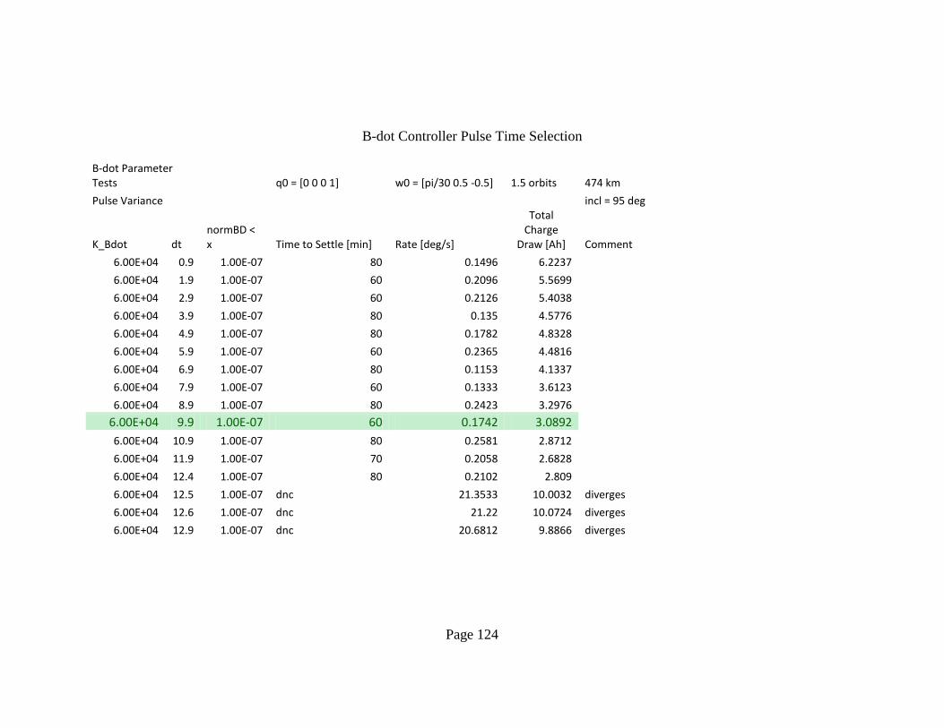
Page 124
B-dot Controller Pulse Time Selection
B-dot Parameter Tests q0 = [0 0 0 1] w0 = [pi/30 0.5 -0.5] 1.5 orbits 474 km
Pulse Variance incl = 95 deg
K_Bdot dt normBD < x Time to Settle [min] Rate [deg/s]
Total Charge
Draw [Ah] Comment
6.00E+04 0.9 1.00E-07 80 0.1496 6.2237
6.00E+04 1.9 1.00E-07 60 0.2096 5.5699
6.00E+04 2.9 1.00E-07 60 0.2126 5.4038
6.00E+04 3.9 1.00E-07 80 0.135 4.5776
6.00E+04 4.9 1.00E-07 80 0.1782 4.8328
6.00E+04 5.9 1.00E-07 60 0.2365 4.4816
6.00E+04 6.9 1.00E-07 80 0.1153 4.1337
6.00E+04 7.9 1.00E-07 60 0.1333 3.6123
6.00E+04 8.9 1.00E-07 80 0.2423 3.2976
6.00E+04 9.9 1.00E-07 60 0.1742 3.0892
6.00E+04 10.9 1.00E-07 80 0.2581 2.8712
6.00E+04 11.9 1.00E-07 70 0.2058 2.6828
6.00E+04 12.4 1.00E-07 80 0.2102 2.809
6.00E+04 12.5 1.00E-07 dnc 21.3533 10.0032 diverges
6.00E+04 12.6 1.00E-07 dnc 21.22 10.0724 diverges
6.00E+04 12.9 1.00E-07 dnc 20.6812 9.8866 diverges

Page 125
B-dot Controller Convergence Criteria Selection
B-dot Parameter Tests q0 = [0 0 0 1] w0 = [pi/30 0.5 -0.5] 5 orbits 475 km
Convergence Criteria Variance incl = 95 deg
K_Bdot dt normBD < x Time to Settle [min] Rate [deg/s]
Total Charge
Draw [Ah] Comment
6.00E+04 9.9 1.00E-07 dnc 0.1684 8.5026
6.00E+04 9.9 2.00E-07 dnc 0.1684 8.5026
6.00E+04 9.9 2.50E-07 dnc 0.1684 8.5026
6.00E+04 9.9 3.00E-07 181.4983 0.1539 3.6621
6.00E+04 9.9 3.50E-07 145.165 0.1757 3.1246
6.00E+04 9.9 4.00E-07 82.165 0.1301 2.13
6.00E+04 9.9 4.50E-07 49.4983 0.307 1.5551
6.00E+04 9.9 5.00E-07 45.8317 0.3464 1.5076
6.00E+04 9.9 5.50E-07 43.4983 0.3783 1.4694
6.00E+04 9.9 6.00E-07 42.165 0.4202 1.4515
6.00E+04 9.9 6.50E-07 39.8317 0.5117 1.417
6.00E+04 9.9 7.00E-07 39.8317 0.5117 1.417
6.00E+04 9.9 7.50E-07 22.8317 0.9337 1.0726
6.00E+04 9.9 8.00E-07 22.8317 0.9337 1.0726
6.00E+04 9.9 8.50E-07 22.8317 0.9337 1.0726
6.00E+04 9.9 9.00E-07 20.4983 0.985 1.035
6.00E+04 9.9 9.50E-07 20.4983 0.985 1.035
6.00E+04 9.9 1.00E-06 20.4983 0.985 1.035
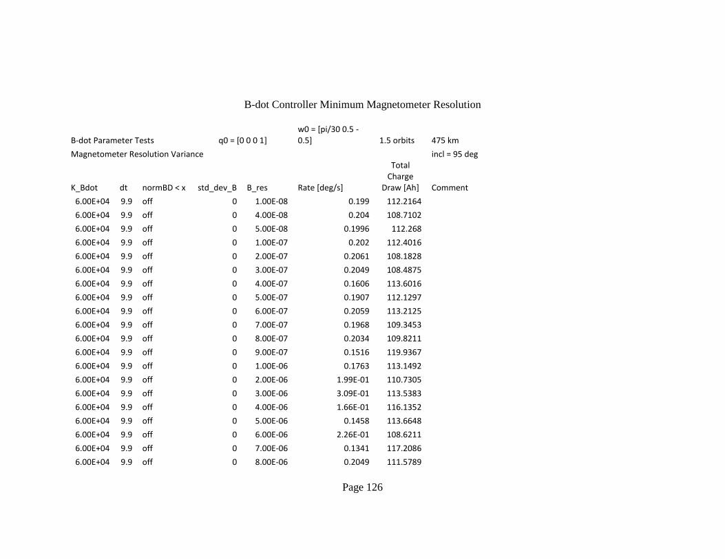
Page 126
B-dot Controller Minimum Magnetometer Resolution
B-dot Parameter Tests q0 = [0 0 0 1] w0 = [pi/30 0.5 -0.5] 1.5 orbits 475 km
Magnetometer Resolution Variance incl = 95 deg
K_Bdot dt normBD < x std_dev_B B_res Rate [deg/s]
Total Charge
Draw [Ah] Comment
6.00E+04 9.9 off 0 1.00E-08 0.199 112.2164
6.00E+04 9.9 off 0 4.00E-08 0.204 108.7102
6.00E+04 9.9 off 0 5.00E-08 0.1996 112.268
6.00E+04 9.9 off 0 1.00E-07 0.202 112.4016
6.00E+04 9.9 off 0 2.00E-07 0.2061 108.1828
6.00E+04 9.9 off 0 3.00E-07 0.2049 108.4875
6.00E+04 9.9 off 0 4.00E-07 0.1606 113.6016
6.00E+04 9.9 off 0 5.00E-07 0.1907 112.1297
6.00E+04 9.9 off 0 6.00E-07 0.2059 113.2125
6.00E+04 9.9 off 0 7.00E-07 0.1968 109.3453
6.00E+04 9.9 off 0 8.00E-07 0.2034 109.8211
6.00E+04 9.9 off 0 9.00E-07 0.1516 119.9367
6.00E+04 9.9 off 0 1.00E-06 0.1763 113.1492
6.00E+04 9.9 off 0 2.00E-06 1.99E-01 110.7305
6.00E+04 9.9 off 0 3.00E-06 3.09E-01 113.5383
6.00E+04 9.9 off 0 4.00E-06 1.66E-01 116.1352
6.00E+04 9.9 off 0 5.00E-06 0.1458 113.6648
6.00E+04 9.9 off 0 6.00E-06 2.26E-01 108.6211
6.00E+04 9.9 off 0 7.00E-06 0.1341 117.2086
6.00E+04 9.9 off 0 8.00E-06 0.2049 111.5789

Page 127
6.00E+04 9.9 off 0 9.00E-06 0.3559 109.9102
6.00E+04 9.9 off 0 1.00E-05 0.6275 120.3094 visible b_body error
6.00E+04 9.9 off 0 1.25E-05 0.1101 116.1633
6.00E+04 9.9 off 0 1.50E-05 0.1917 116.2148
6.00E+04 9.9 off 0 1.75E-05 0.2819 134.6039
6.00E+04 9.9 off 0 2.00E-05 0.17 133.8914 step behavior in yaw rates
6.00E+04 9.9 off 0 2.25E-05 0.3362 116.2336
6.00E+04 9.9 off 0 2.50E-05 0.3983 132.8484
6.00E+04 9.9 off 0 2.75E-05 0.2737 117.7688
6.00E+04 9.9 off 0 3.00E-05 0.8892 122.6109
6.00E+04 9.9 off 0 3.25E-05 0.8076 122.3531
6.00E+04 9.9 off 0 3.50E-05 0.3192 130.7836
6.00E+04 9.9 off 0 3.75E-05 0.1544 145.5656
6.00E+04 9.9 off 0 4.00E-05 0.1862 126.1594
6.00E+04 9.9 off 0 4.25E-05 0.9482 132.2578
6.00E+04 9.9 off 0 4.50E-05 0.3845 103.425
6.00E+04 9.9 off 1 4.75E-05 0.4814 112.1578
6.00E+04 9.9 off 0 5.00E-05 27.2824 424.1391 complete divergence

Page 128
B-dot Controller Maximum Magnetometer Noise
B-dot Parameter Tests q0 = [0 0 0 1] w0 = [pi/30 0.5 -0.5] 1.5 orbits 475 km
Magnetometer Noise Variance incl = 95 deg
K_Bdot dt normBD < x std_dev_B B_res Rate [deg/s]
Total Charge
Draw [Ah] Comment
6.00E+04 9.9 off 0 1.00E-07 0.202 112.4016
6.00E+04 9.9 off 1.00E-07 1.00E-07 0.1942 111.832
6.00E+04 9.9 off 2.00E-07 1.00E-07 0.2012 112.9875
6.00E+04 9.9 off 3.00E-07 1.00E-07 0.2085 108.0844
6.00E+04 9.9 off 4.00E-07 1.00E-07 0.1906 111.3539
6.00E+04 9.9 off 5.00E-07 1.00E-07 0.1795 110.2125
6.00E+04 9.9 off 6.00E-07 1.00E-07 0.2478 112.1109
6.00E+04 9.9 off 7.00E-07 1.00E-07 0.146 115.6148
6.00E+04 9.9 off 8.00E-07 1.00E-07 0.2684 111.9563
6.00E+04 9.9 off 9.00E-07 1.00E-07 0.2334 115.0805
6.00E+04 9.9 off 1.00E-06 1.00E-07 0.1979 112.3195
6.00E+04 9.9 off 2.00E-06 1.00E-07 0.2159 128.9531
6.00E+04 9.9 off 3.00E-06 1.00E-07 0.2898 145.4508
6.00E+04 9.9 off 4.00E-06 1.00E-07 0.099 165.1945
6.00E+04 9.9 off 5.00E-06 1.00E-07 0.4206 187.132
6.00E+04 9.9 off 6.00E-06 1.00E-07 0.1371 209.6156
6.00E+04 9.9 off 7.00E-06 1.00E-07 0.6753 229.95
6.00E+04 9.9 off 8.00E-06 1.00E-07 0.3291 249.5672
6.00E+04 9.9 off 9.00E-06 1.00E-07 0.3857 270.1406
6.00E+04 9.9 off 1.00E-05 1.00E-07 0.5896 305.2711

Page 129
6.00E+04 9.9 off 1.50E-05 1.00E-07 1.0227 406.2445
6.00E+04 9.9 off 2.00E-05 1.00E-07 1.1139 503.0883
6.00E+04 9.9 off 2.50E-05 1.00E-07 1.4743 581.625
6.00E+04 9.9 off 3.00E-05 1.00E-07 0.9003 635.9953
6.00E+04 9.9 off 3.50E-05 1.00E-07 27.3258 726.7031 Complete Divergence
6.00E+04 9.9 off 4.00E-05 1.00E-07 1.9434 679.3078 Local instabilities
6.00E+04 9.9 off 4.50E-05 1.00E-07 25.5334 756.5883 Complete Divergence
6.00E+04 9.9 off 5.00E-05 1.00E-07 26.2234 736.2234 Complete Divergence
6.00E+04 9.9 off 1.00E-04 1.00E-07 2.76E+01 8.55E+02 Complete Divergence
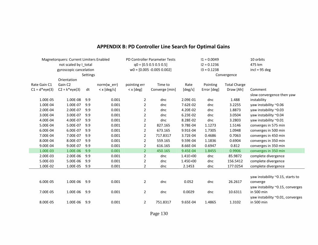
Page 130
APPENDIX B: PD Controller Line Search for Optimal Gains
Magnetorquers: Current Limiters Enabled PD Controller Parameter Tests I1 = 0.0049 10 orbits
not scaled by I_total q0 = [0.5 0.5 0.5 0.5] I2 = 0.1236 475 km
gyroscopic cancelation w0 = [0.005 -0.005 0.002] I3 = 0.1238 incl = 95 deg
Settings Convergence
Rate Gain C1 C1 = d*eye(3)
Orientation Gain C2 C2 = k*eye(3) dt
norm(w_err) < x [deg/s]
pointing err < x [deg]
Time to Converge [min]
Rate [deg/s]
Pointing Error [deg]
Total Charge Draw [Ah] Comment
1.00E-05 1.00E-08 9.9 0.001 2 dnc 2.09E-01 dnc 1.488 slow convergence then yaw instability
1.00E-04 1.00E-07 9.9 0.001 2 dnc 7.62E-02 dnc 3.2255 yaw instability ~0.06
2.00E-04 2.00E-07 9.9 0.001 2 dnc 4.20E-02 dnc 1.8873 yaw instability ~0.03
3.00E-04 3.00E-07 9.9 0.001 2 dnc 6.23E-02 dnc 3.0504 yaw instability ~0.04
4.00E-04 4.00E-07 9.9 0.001 2 dnc 8.28E-02 dnc 3.2803 yaw instability ~0.01
5.00E-04 5.00E-07 9.9 0.001 2 827.165 9.78E-04 1.1273 1.5146 converges in 575 min
6.00E-04 6.00E-07 9.9 0.001 2 673.165 9.91E-04 1.7305 1.0948 converges in 500 min
7.00E-04 7.00E-07 9.9 0.001 2 717.8317 3.72E-04 0.4686 0.7063 converges in 450 min
8.00E-04 8.00E-07 9.9 0.001 2 559.165 9.59E-04 1.1836 0.6904 converges in 350 min
9.00E-04 9.00E-07 9.9 0.001 2 616.165 8.66E-04 0.6947 0.812 converges in 350 min
1.00E-03 1.00E-06 9.9 0.001 2 450.165 9.45E-04 1.8455 0.9906 converges in 350 min
2.00E-03 2.00E-06 9.9 0.001 2 dnc 1.41E+00 dnc 85.9872 complete divergence
5.00E-03 5.00E-06 9.9 0.001 2 dnc 1.45E+00 dnc 156.5412 complete divergence
1.00E-02 1.00E-05 9.9 0.001 2 dnc 2.1453 dnc 177.0254 complete divergence
6.00E-05 1.00E-06 9.9 0.001 2 dnc 0.052 dnc 26.2617 yaw instability ~0.15, starts to converge
7.00E-05 1.00E-06 9.9 0.001 2 dnc 0.0029 dnc 10.6311 yaw instability ~0.15, converges in 500 min
8.00E-05 1.00E-06 9.9 0.001 2 751.8317 9.65E-04 1.4865 1.3102 yaw instability ~0.01, converges in 500 min

Page 131
9.00E-05 1.00E-06 9.9 0.001 2 dnc 0.0098 dnc 1.3714 yaw instability ~0.01, converges in 350 min
1.00E-04 1.00E-06 9.9 0.001 2 716.165 9.82E-04 1.7298 8.6956 yaw instability ~0.01, converges in 450 min
2.00E-04 1.00E-06 9.9 0.001 2 488.8317 9.85E-04 0.9875 1.0926 converges in 350 min
3.00E-04 1.00E-06 9.9 0.001 2 570.165 9.73E-04 1.7534 0.8962 converges in 450 min
4.00E-04 1.00E-06 9.9 0.001 2 622.165 8.74E-04 1.5489 0.7821 converges in 250 min
5.00E-04 1.00E-06 9.9 0.001 2 613.4983 7.58E-04 0.8117 0.5025 converges in 125 min
6.00E-04 1.00E-06 9.9 0.001 2 571.165 8.70E-04 1.8629 0.732 converges in 450 min
7.00E-04 1.00E-06 9.9 0.001 2 551.165 9.89E-04 0.9282 0.7313 converges in 150 min
8.00E-04 1.00E-06 9.9 0.001 2 570.8317 9.79E-04 0.8323 0.7265 converges in 250 min
9.00E-04 1.00E-06 9.9 0.001 2 439.165 8.76E-04 1.0468 0.7636 converges in 325 min
1.00E-03 1.00E-06 9.9 0.001 2 450.165 9.45E-04 1.8455 0.9906 converges in 350 min
2.00E-03 1.00E-06 9.9 0.001 2 dnc 1.52E-01 dnc 83.7954 diverges
3.00E-03 1.00E-06 9.9 0.001 2 dnc 3.46E-02 dnc 135.5382 diverges
9.00E-04 9.00E-07 9.9 0.001 2 616.165 8.66E-04 0.6947 0.812 converges in 350 min
9.00E-04 1.00E-06 9.9 0.001 2 439.165 8.76E-04 1.0468 0.7636 converges in 325 min
9.00E-04 2.00E-06 9.9 0.001 2 438.165 8.90E-04 0.7477 0.863 converges in 200 min
9.00E-04 3.00E-06 9.9 0.001 2 341.165 5.80E-04 0.5987 0.8867 converges in 150 min
9.00E-04 4.00E-06 9.9 0.001 2 302.165 9.68E-04 0.8217 2.9356 converges in 250 min
9.00E-04 5.00E-06 9.9 0.001 2 617.4983 4.80E-04 1.0165 4.3888 converges in 425 min
9.00E-04 6.00E-06 9.9 0.001 2 392.4983 9.88E-04 0.7407 2.7669 converges in 300 min
9.00E-04 7.00E-06 9.9 0.001 2 666.8317 9.30E-04 0.702 10.932 converges in 600 min
4.00E-04 4.00E-06 9.9 0.001 2 716.4983 9.98E-04 0.4633 7.0095 converges in 500 min
5.00E-04 4.00E-06 9.9 0.001 2 258.8317 8.50E-04 0.766 4.9479 converges in 175 min
6.00E-04 4.00E-06 9.9 0.001 2 302.4983 9.80E-04 0.9661 1.8418 converges in 250 min
7.00E-04 4.00E-06 9.9 0.001 2 618.4983 9.17E-04 0.9011 4.5161 converges in 425 min
8.00E-04 4.00E-06 9.9 0.001 2 197.165 5.74E-04 0.7537 1.1883 converges in 100 min
9.00E-04 4.00E-06 9.9 0.001 2 302.165 9.68E-04 0.8217 2.9356 converges in 250 min

Page 132
1.00E-03 4.00E-06 9.9 0.001 2 435.8317 9.99E-04 1.2235 4.3806 converges in 400 min
2.00E-03 4.00E-06 9.9 0.001 2 dnc 0.6669 dnc 55.0658 yaw instability ~0.05
8.00E-04 3.00E-06 9.9 0.001 2 616.165 1.00E-03 0.5892 4.2469 converges in 450 min
8.00E-04 4.00E-06 9.9 0.001 2 197.165 0.000574 0.7537 1.1883 converges in 100 min
8.00E-04 5.00E-06 9.9 0.001 2 193.4983 8.43E-04 1.1333 1.0403 converges in 125 min
8.00E-04 6.00E-06 9.9 0.001 2 298.8317 8.99E-04 0.5819 1.2835 converges in 150 min
8.00E-04 7.00E-06 9.9 0.001 2 426.165 8.12E-04 0.8746 5.6192 converges in 350 min
7.00E-04 5.00E-06 9.9 0.001 2 255.4983 4.82E-04 1.4353 2.8671 converges in 200 min
8.00E-04 5.00E-06 9.9 0.001 2 197.165 0.000574 0.7537 1.1883 converges in 100 min
9.00E-04 5.00E-06 9.9 0.001 2 617.4983 4.80E-04 1.0165 4.3888 converges in 450 min
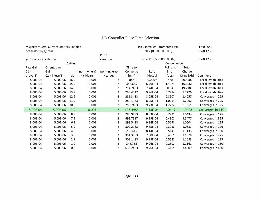
Page 133
PD Controller Pulse Time Selection
Magnetorquers: Current Limiters Enabled PD Controller Parameter Tests I1 = 0.0049
not scaled by I_total q0 = [0.5 0.5 0.5 0.5] I2 = 0.1236
gyroscopic cancelation
Pulse variation w0 = [0.005 -0.005 0.002] I3 = 0.1238
Settings Convergence Rate Gain C1 = d*eye(3)
Orientation Gain C2 = k*eye(3) dt
norm(w_err) < x [deg/s]
pointing error < x [deg]
Time to Converge
[min] Rate
[deg/s]
Pointing Error [deg]
Total Charge
Draw [Ah] Comment
8.00E-04 5.00E-06 16.9 0.001 2 dnc 0.0269 dnc 40.5502 Local instabilities
8.00E-04 5.00E-06 15.9 0.001 2 382.665 6.76E-04 1.4074 16.2061 Local instabilities
8.00E-04 5.00E-06 14.9 0.001 2 714.7483 7.44E-04 0.34 19.2183 Local instabilities
8.00E-04 5.00E-06 13.9 0.001 2 298.4317 9.96E-04 0.7914 1.7226 Local instabilities
8.00E-04 5.00E-06 12.9 0.001 2 285.3483 8.05E-04 0.8907 1.4057 Converges in 225
8.00E-04 5.00E-06 11.9 0.001 2 284.1983 8.25E-04 1.0054 1.2062 Converges in 225
8.00E-04 5.00E-06 10.9 0.001 2 255.7483 9.73E-04 1.2234 1.092 Converges in 125
8.00E-04 5.00E-06 9.9 0.001 2 193.4983 8.43E-04 1.0445 1.0403 Converges in 110 8.00E-04 5.00E-06 8.9 0.001 2 283.9483 8.03E-04 0.7222 1.0434 Converges in 125
8.00E-04 5.00E-06 7.9 0.001 2 493.7317 9.99E-04 0.4902 3.5477 Converges in 325
8.00E-04 5.00E-06 6.9 0.001 2 298.5483 9.84E-04 0.5178 1.0604 Converges in 125
8.00E-04 5.00E-06 5.9 0.001 2 300.2983 9.85E-04 0.3918 1.0687 Converges in 126
8.00E-04 5.00E-06 4.9 0.001 2 212.415 8.14E-04 0.5141 1.1133 Converges in 100
8.00E-04 5.00E-06 3.9 0.001 2 351.3983 7.90E-04 0.4805 1.1878 Converges in 225
8.00E-04 5.00E-06 2.9 0.001 2 303.1483 9.99E-04 0.5532 1.1083 Converges in 125
8.00E-04 5.00E-06 1.9 0.001 2 348.765 9.96E-04 0.2502 1.1161 Converges in 150
8.00E-04 5.00E-06 0.9 0.001 2 630.2483 9.76E-04 0.4109 3.4209 Converges in 400
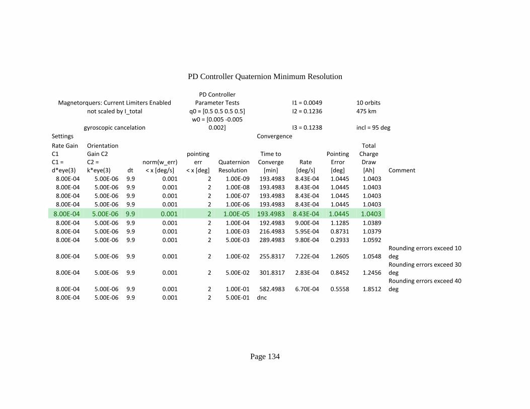
Page 134
PD Controller Quaternion Minimum Resolution
Magnetorquers: Current Limiters Enabled PD Controller
Parameter Tests I1 = 0.0049 10 orbits
not scaled by I_total q0 = [0.5 0.5 0.5 0.5] I2 = 0.1236 475 km
gyroscopic cancelation w0 = [0.005 -0.005
0.002] I3 = 0.1238 incl = 95 deg
Settings Convergence
Rate Gain C1 C1 = d*eye(3)
Orientation Gain C2 C2 = k*eye(3) dt
norm(w_err) < x [deg/s]
pointing err
< x [deg] Quaternion Resolution
Time to Converge
[min] Rate
[deg/s]
Pointing Error [deg]
Total Charge Draw [Ah] Comment
8.00E-04 5.00E-06 9.9 0.001 2 1.00E-09 193.4983 8.43E-04 1.0445 1.0403
8.00E-04 5.00E-06 9.9 0.001 2 1.00E-08 193.4983 8.43E-04 1.0445 1.0403
8.00E-04 5.00E-06 9.9 0.001 2 1.00E-07 193.4983 8.43E-04 1.0445 1.0403
8.00E-04 5.00E-06 9.9 0.001 2 1.00E-06 193.4983 8.43E-04 1.0445 1.0403
8.00E-04 5.00E-06 9.9 0.001 2 1.00E-05 193.4983 8.43E-04 1.0445 1.0403 8.00E-04 5.00E-06 9.9 0.001 2 1.00E-04 192.4983 9.00E-04 1.1285 1.0389
8.00E-04 5.00E-06 9.9 0.001 2 1.00E-03 216.4983 5.95E-04 0.8731 1.0379
8.00E-04 5.00E-06 9.9 0.001 2 5.00E-03 289.4983 9.80E-04 0.2933 1.0592
8.00E-04 5.00E-06 9.9 0.001 2 1.00E-02 255.8317 7.22E-04 1.2605 1.0548 Rounding errors exceed 10 deg
8.00E-04 5.00E-06 9.9 0.001 2 5.00E-02 301.8317 2.83E-04 0.8452 1.2456 Rounding errors exceed 30 deg
8.00E-04 5.00E-06 9.9 0.001 2 1.00E-01 582.4983 6.70E-04 0.5558 1.8512 Rounding errors exceed 40 deg
8.00E-04 5.00E-06 9.9 0.001 2 5.00E-01 dnc

Page 135
PD Controller Quaternion Maximum Noise
Magnetorquers: Current Limiters Enabled PD Controller
Parameter Tests I1 = 0.0049 10 orbits
not scaled by I_total q0 = [0.5 0.5 0.5 0.5] I2 = 0.1236 475 km
gyroscopic cancelation w0 = [0.005 -0.005
0.002] I3 = 0.1238
incl = 95 deg
Settings Convergence
Rate C1 = d*eye(3)
Orientation C2 = k*eye(3) dt
norm(w_err) < x [deg/s]
pointing err
< x [deg]
Quaternion Noise std_dev
Time to Converge
[min] Rate
[deg/s]
Pointing Error [deg]
Total Charge
Draw [Ah] Comment
8.00E-04 5.00E-06 9.9 0.001 2 1.00E-09 193.4983 8.43E-04 1.0445 1.0403
8.00E-04 5.00E-06 9.9 0.001 2 1.00E-08 193.4983 8.43E-04 1.0445 1.0403
8.00E-04 5.00E-06 9.9 0.001 2 1.00E-07 193.4983 8.43E-04 1.0445 1.0403
8.00E-04 5.00E-06 9.9 0.001 2 1.00E-06 193.4983 8.43E-04 1.0445 1.0403
8.00E-04 5.00E-06 9.9 0.001 2 1.00E-05 193.4983 8.38E-04 1.0424 1.0405
8.00E-04 5.00E-06 9.9 0.001 2 1.00E-04 255.4983 4.97E-04 1.0494 1.046 noise ~2 deg
8.00E-04 5.00E-06 9.9 0.001 2 1.00E-03 261.8317 7.67E-04 0.5052 1.0423 noise ~8 deg
8.00E-04 5.00E-06 9.9 0.001 2 5.00E-03 282.4983 9.64E-04 0.6745 1.1041 noise ~15 deg
8.00E-04 5.00E-06 9.9 0.001 2 1.00E-02 151.8317 9.59E-04 0.6124 1.0891 noise ~21 deg
8.00E-04 5.00E-06 9.9 0.001 2 5.00E-02 769.8317 9.69E-04 2.7363 3.4052 noise ~60 deg
8.00E-04 5.00E-06 9.9 0.001 2 1.00E-01 dnc 1.17E-01 dnc 12.1235

Page 136
PD Controller Rate Minimum Resolution
Magnetorquers: Current Limiters Enabled PD Controller
Parameter Tests I1 = 0.0049 10 orbits
not scaled by I_total q0 = [0.5 0.5 0.5 0.5] I2 = 0.1236 475 km
gyroscopic cancelation w0 = [0.005 -0.005
0.002] I3 = 0.1238 incl = 95 deg
Settings Convergence
Rate Gain C1 C1 = d*eye(3)
Orientation Gain C2 C2 = k*eye(3) dt
norm(w_err) < x [deg/s]
pointing err
< x [deg]
Rate Resolution [rad/s]
Time to Converge
[min] Rate
[deg/s]
Pointing Error [deg]
Total Charge Draw [Ah] Comment
8.00E-04 5.00E-06 9.9 0.001 2 1.00E-09 193.4983 8.43E-04 1.0445 1.0403
8.00E-04 5.00E-06 9.9 0.001 2 1.00E-08 193.4983 8.43E-04 1.0445 1.0403
8.00E-04 5.00E-06 9.9 0.001 2 1.00E-07 193.4983 8.43E-04 1.0445 1.0403
8.00E-04 5.00E-06 9.9 0.001 2 1.00E-06 192.165 9.64E-04 1.5354 1.0345
8.00E-04 5.00E-06 9.9 0.001 2 1.00E-05 284.165 0.001 0.8512 1.0602 8.00E-04 5.00E-06 9.9 0.001 2 1.00E-04 159.8317 3.90E-03 1.8298 1.0503
8.00E-04 5.00E-06 9.9 0.001 2 5.00E-04 dnc 7.00E-03 dnc 1.96
8.00E-04 5.00E-06 9.9 0.001 2 1.00E-03 dnc 0.0142 dnc 3.3373

Page 137
PD Controller Rate Maximum Noise
Magnetorquers: Current Limiters Enabled PD Controller
Parameter Tests I1 = 0.0049 10 orbits
not scaled by I_total q0 = [0.5 0.5 0.5 0.5] I2 = 0.1236 475 km
gyroscopic cancelation w0 = [0.005 -0.005
0.002] I3 = 0.1238 incl = 95 deg
Settings Convergence
Rate Gain C1 C1 = d*eye(3)
Orientation Gain C2 C2 = k*eye(3) dt
norm(w_err) < x [deg/s]
pointing err
< x [deg] Rate noise [rad/s]
Time to Converge
[min] Rate
[deg/s]
Pointing Error [deg]
Total Charge Draw [Ah] Comment
8.00E-04 5.00E-06 9.9 0.001 2 1.00E-09 193.4983 8.43E-04 1.0445 1.0403
8.00E-04 5.00E-06 9.9 0.001 2 1.00E-08 193.4983 8.43E-04 1.0445 1.0403
8.00E-04 5.00E-06 9.9 0.001 2 1.00E-07 256.4983 3.65E-04 0.9758 1.0428
8.00E-04 5.00E-06 9.9 0.001 2 1.00E-06 255.165 5.52E-04 0.572 1.0436
8.00E-04 5.00E-06 9.9 0.001 2 1.00E-05 241.165 9.56E-04 0.834 1.0459 8.00E-04 5.00E-06 9.9 0.001 2 1.00E-04 247.8317 9.30E-03 1.0238 1.1885
8.00E-04 5.00E-06 9.9 0.001 2 5.00E-04 dnc 5.32E-02 dnc 5.9397
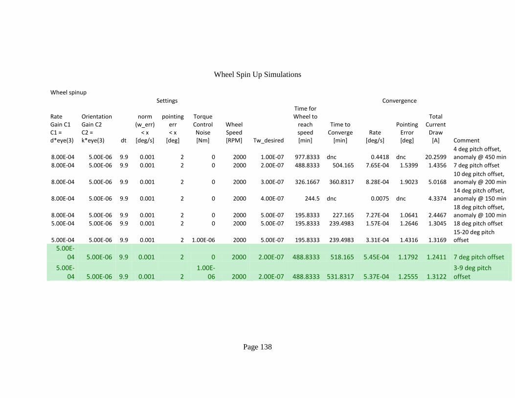
Page 138
Wheel Spin Up Simulations
Wheel spinup
Settings Convergence
Rate Gain C1 C1 = d*eye(3)
Orientation Gain C2 C2 = k*eye(3) dt
norm (w_err)
< x [deg/s]
pointing err < x
[deg]
Torque Control Noise [Nm]
Wheel Speed [RPM] Tw_desired
Time for Wheel to
reach speed [min]
Time to Converge
[min] Rate
[deg/s]
Pointing Error [deg]
Total Current
Draw [A] Comment
8.00E-04 5.00E-06 9.9 0.001 2 0 2000 1.00E-07 977.8333 dnc 0.4418 dnc 20.2599 4 deg pitch offset, anomaly @ 450 min
8.00E-04 5.00E-06 9.9 0.001 2 0 2000 2.00E-07 488.8333 504.165 7.65E-04 1.5399 1.4356 7 deg pitch offset
8.00E-04 5.00E-06 9.9 0.001 2 0 2000 3.00E-07 326.1667 360.8317 8.28E-04 1.9023 5.0168 10 deg pitch offset, anomaly @ 200 min
8.00E-04 5.00E-06 9.9 0.001 2 0 2000 4.00E-07 244.5 dnc 0.0075 dnc 4.3374 14 deg pitch offset, anomaly @ 150 min
8.00E-04 5.00E-06 9.9 0.001 2 0 2000 5.00E-07 195.8333 227.165 7.27E-04 1.0641 2.4467 18 deg pitch offset, anomaly @ 100 min
5.00E-04 5.00E-06 9.9 0.001 2 0 2000 5.00E-07 195.8333 239.4983 1.57E-04 1.2646 1.3045 18 deg pitch offset
5.00E-04 5.00E-06 9.9 0.001 2 1.00E-06 2000 5.00E-07 195.8333 239.4983 3.31E-04 1.4316 1.3169 15-20 deg pitch offset
5.00E-04 5.00E-06 9.9 0.001 2 0 2000 2.00E-07 488.8333 518.165 5.45E-04 1.1792 1.2411 7 deg pitch offset
5.00E-04 5.00E-06 9.9 0.001 2
1.00E-06 2000 2.00E-07 488.8333 531.8317 5.37E-04 1.2555 1.3122
3-9 deg pitch offset