A Gradient-Based Comparison Measure for Visual...

Eurographics / IEEE Symposium on Visualization 2011 (EuroVis 2011)H. Hauser, H. Pfister, and J. J. van Wijk(Guest Editors)

Volume 30 (2011), Number 3

A Gradient-Based Comparison Measure for Visual analysis of

Multifield Data

Suthambhara Nagaraj1, Vijay Natarajan1,2, and Ravi S. Nanjundiah3

1Department of Computer Science and Automation, Indian Institute of Science, Bangaloreemail: {suthambhara,vijayn}@csa.iisc.ernet.in

2Supercomputer Education and Research Center, Indian Institute of Science, Bangalore3Centre for Atmospheric and Oceanic Sciences, Indian Institute of Science, Bangalore

email: [email protected]

Abstract

We introduce a multifield comparison measure for scalar fields that helps in studying relations between them. The

comparison measure is insensitive to noise in the scalar fields and to noise in their gradients. Further, it can be

computed robustly and efficiently. Results from the visual analysis of various data sets from climate science and

combustion applications demonstrate the effective use of the measure.

Categories and Subject Descriptors (according to ACM CCS): I.3.6 [Computer Graphics]: Computer Graphics—Methodology and Techniques

1. Introduction

Data from present day simulations and observations of phys-ical processes often consists of multiple scalar and vectorfields. Studying the interactions between the fields is pivotalto understanding the underlying phenomenon.

Single scalar fields are typically studied using tech-niques like isosurfacing, direct volume rendering and con-tour trees [HJ04,SML06,PWH01,CSvdP04,CSA00]. Whenvisualizing multiple scalar fields, the above methods can beused separately on each field and visualized side by side oras overlays. The relationships and interactions that exist be-tween the fields are often not captured by such methods. Si-multaneous visualization of all the fields facilitates the un-derstanding of interactions and relationships between them.This can be accomplished by employing a comparative ap-proach to capture the relationships between variables.

We present a new gradient-based comparison measure forscalar fields that is applicable on an arbitrary number ofscalar fields defined on a manifold. The measure captures theextent of alignment of the gradient vectors at a point. Thedistribution of the measure over the domain provides keyinsights into the interaction between input fields. The mea-sure satisfies various desirable mathematical properties, canbe computed efficiently, and is practically useful for study-ing relationships between multiple scalar fields. Our team of

visualization researchers and a climate scientist worked to-gether to apply this measure for analyzing a hurricane simu-lation data set and a global climate simulation data set. Theanalysis helps explain various known meteorological and cli-matic phenomena. We also demonstrate the effective use ofan aggregated version of the measure to the study of a com-bustion simulation data set.

The main contributions of this paper are :

• A new multifield comparison measure to capture inter-actions between multiple scalar fields defined on an n-dimensional domain,

• Theoretical results that establish the robustness of themeasure by showing its insensitivity to noise in the scalarfields,

• An algorithm to compute the measure efficiently, and• Real world applications to demonstrate the effectiveness

of the measure in studying interactions between scalarfields in physical phenomena and an extension to vectorfields.

The rest of the paper is organized as follows. We describeprevious work in Section 2. In Section 3, we define the multi-field comparison measure and prove its robustness and otherproperties. We motivate the use of the measure and explainits working in Section 4. Computation of the measure is de-scribed in Section 5. We describe several applications of the

c© 2011 The Author(s)

Journal compilation c© 2011 The Eurographics Association and Blackwell Publishing Ltd.

Published by Blackwell Publishing, 9600 Garsington Road, Oxford OX4 2DQ, UK and

350 Main Street, Malden, MA 02148, USA.

110 / A Gradient-Based Comparison Measure for Visual analysis of Multifield Data

measure in Section 6. In Section 7, we discuss the limitationsof the multifield comparison measure and its insensitivity tonoise in a real world data. We conclude the paper in Sec-tion 8.

2. Related Work

A popular approach to visualizing multiple fields is to com-bine them into a single value and then render the combinedvolume [CS99, BPRS98]. Woodring et al. [WS06] proposethat the data fields should be rendered together within thesame space for user comparison. They use set operators tocombine the different fields into a single field that extractsthe interesting portions of the data. These set operators caneither combine the color values of the input fields or di-rectly apply the operation in data space. Though combin-ing volumes shows important parts of the data, the interac-tions between the different variables that are of importanceto the domain scientists are not captured. For multifield timevarying data, Lee et al. [LS09] propose a linear time algo-rithm to extract trend relationships among variables basedon studying the change of variables over time and how thesechanges are related among different variables. Features inmultifield data have been extracted using techniques likescatter plots [BW08] and variation density plots [NN10].

Multifield data have also been studied using statisticalmethods. One important work in this area uses the local sta-tistical complexity [JWSK07] to identify features which mayexhibit the same behavior in the future. Features are identi-fied as complex if the probability that they occur again is low.In a later work, Jänicke et al. [JBTS08] improve the accuracyand efficiency of computing the local statistical complexity.

The relationship between the different scalar fields is pop-ularly captured with the help of correlation measures. Sauberet al. [STS06] use two different techniques to compare dif-ferent scalar fields at a point. One of them uses the alignmentof gradients of the fields and also their magnitudes as a cri-terion to measure similarity. When the number of fields ex-ceed two, pairwise similarity is computed and the least valueis considered. This would detect regions where two of thefields are highly correlated. An obvious limitation of this ap-proach is that two highly correlated fields would result in theother fields of the data to be ignored. In the same paper, theauthors also describe a local correlation coefficient to detectlinear dependencies between the scalar fields. The advantageof this method is its insensitivity to scaling of the data fields.It also has the same limitation as the first approach. Gosinket al. [GAJ07] also use correlation fields to study the inter-actions between the different variables in multi-field data.The inner product of the gradients of two fields of interest iscomputed over principle level sets of a third field. They usethis approach to study combustion in methane and hydrogen.A limitation with using the inner product of the gradients isthat only two fields can be compared.

Edelsbrunner et al. [EHNP04] also employ a gradient-

based approach to measure relationships between scalarfields. In their work, they introduce a measure to comparemultiple scalar fields both locally at a point as well as overa region of the domain. In the case of three dimensional Eu-clidean space and two fields, they show that the measure at apoint reduces to the length of cross product of the gradientsof the fields. This measure, though useful, has a limitationthat the number of scalar fields that can be compared cannotexceed the dimension of the domain.

In this paper, we also explore a gradient-based approachto compare scalar fields locally at a point. However, ourmethod is not limited by the number of fields that can becompared unlike previous approaches. Our method also ex-tends to time-varying scalar fields and to vector fields. Fur-ther, the measure is provably robust to noise in the inputfields.

3. Multifield Comparison Measure

In this section, we introduce a gradient-based comparisonmeasure for multiple scalar functions. The measure is de-fined as the norm of a matrix comprising the gradient vectorsof the different functions. We first define the matrix normbefore defining the measure and listing and proving its prop-erties.

3.1. Matrix Norm

Let A be a m× n matrix of real numbers. The norm of thematrix A, denoted as ‖A‖, is defined as

‖A‖ = max‖x‖=1, x∈Rn

‖Ax‖,

where ‖x‖ represents the Euclidean norm of vector x [HJ85].We list four properties of the matrix norm that we will uselater to prove key properties of the comparison measure. Inparticular, if A and B are matrices of real numbers, then

1. ‖A‖ > 0 if A 6= 0 and ‖A‖ = 0 iff A = 0.2. For α ∈ R, ‖αA‖ = |α |‖A‖.3. ‖A+B‖ ≤ ‖A‖+‖B‖ and ‖A−B‖ ≥ |‖A‖−‖B‖|4. ‖AB‖ ≤ ‖A‖‖B‖.

3.2. Comparison Measure

Let M be a compact Riemannian manifold of dimension n.Let (x1,x2, . . . ,xn) be a local coordinate system such that theunit tangent vectors form an orthonormal basis with respectto the Riemannian metric. Let F = { f1, f2, f3, . . . , fm} be aset of smooth functions defined on the manifold. The deriva-tive at a point p ∈ M is written as a matrix of partial deriva-tives,

dF(p) =

∂ f1

∂x1(p) . . .

∂ f1

∂xn(p)

.... . .

...∂ fm

∂x1(p) . . .

∂ fm

∂xn(p)




X

Y

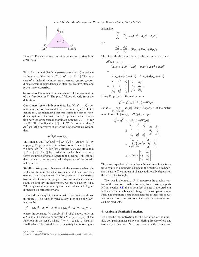
Figure 1: Piecewise-linear function defined on a triangle ina 2D mesh.

We define the multifield comparison measure ηFp at point p

as the norm of the matrix dF(p), ηFp = ‖dF(p)‖. The mea-

sure ηFp satisfies three important properties: symmetry, coor-

dinate system independence and stability. We now state andprove these properties.

Symmetry. The measure is independent of the permutationof the functions in F . The proof follows directly from thedefinition.

Coordinate system independence. Let (x′1,x′2, . . . ,x

′n) de-

note a second orthonormal local coordinate system. Let J

denote the Jacobian matrix that transforms the second coor-dinate system to the first. Since J represents a transforma-tion between orthonormal coordinate systems, |Jv| = |v| forv ∈ R

n. This implies that ‖J‖ = 1. We first observe that ifdF ′(p) is the derivative at p for the new coordinate system,then,

dF ′(p) = dF(p)J.

This implies that ‖dF ′(p)‖ = ‖dF(p)J‖ ≤ ‖dF(p)‖‖J‖ byapplying Property 4 of the matrix norm. Since ‖J‖ = 1,we have ‖dF ′(p)‖ ≤ ‖dF(p)‖. Similarly, we can prove that‖dF(p)‖≤ ‖dF ′(p)‖ by considering the Jacobian that trans-forms the first coordinate system to the second. This impliesthat the matrix norms are equal independent of the coordi-nate system.

Stability. We prove robustness of the measure when thescalar functions in the set F are piecewise-linear functionsdefined on a triangle mesh. We first observe that the deriva-tive in the interior of a triangle is well defined and is a con-stant. To simplify the description, we prove stability for a2D triangle mesh representing a surface. Extension to higherdimensions is straightforward.

Consider a triangle in the mesh with coordinates as shownin Figure 1. The function value at any interior point p(x,y)is given by

fpi = (A1 f 1

i +A2 f 2i +A3 f 3

i )x+(B1 f 1i +B2 f 2

i +B3 f 3i )y,

where the constants (A1,A2,A3,B1,B2,B3) depend only ona,b, and c. Consider a perturbation F = { f1, . . . , fm} of thefunctions in the set F , where fi = fi + εi and εi assumessmall values. The partial derivatives satisfy the following re-

lationship:

∂ fi

∂x− ∂ fi

∂x= (A1ε1

i +A2ε2i +A3ε3

i )

and

∂ fi

∂y− ∂ fi

∂y= (B1ε1

i +B2ε2i +B3ε3

i ).

Therefore, the difference between the derivative matrices is

dF(p)−dF(p)

=

A1ε11 +A2ε2

1 +A3ε31 B1ε1

1 +B2ε21 +B3ε3

1...

...A1ε1

m +A2ε2m +A3ε3

m B1ε1m +B2ε2

m +B3ε3m

=

ε11 ε2

1 ε31

......

...ε1

m ε2m ε3

m

A1 B1

A2 B2

A3 B3

.

Using Property 3 of the matrix norm,

|ηFp −ηF

p | ≤ ‖dF(p)−dF(p)‖.

Let ε = sup1≤i≤m,p∈M

|εi(p)|. Using Property 4 of the matrix

norm to rewrite ‖dF(p)−dF(p)‖, we get

|ηFp −ηF

p | ≤ ‖dF(p)−dF(p)‖

≤

∥

∥

∥

∥

∥

∥

∥

ε11 ε2

1 ε31

......

...ε1

m ε2m ε3

m

∥

∥

∥

∥

∥

∥

∥

∥

∥

∥

∥

∥

∥

A1 B1

A2 B2

A3 B3

∥

∥

∥

∥

∥

∥

≤

√

√

√

√

m

∑i=1

3

∑j=1

(εj

i )2

∥

∥

∥

∥

∥

∥

A1 B1

A2 B2

A3 B3

∥

∥

∥

∥

∥

∥

≤ (√

3m)ε

∥

∥

∥

∥

∥

∥

A1 B1

A2 B2

A3 B3

∥

∥

∥

∥

∥

∥

.

The above equation indicates that a finite change in the func-tions results in a bounded change in the multifield compari-son measure. The amount of change additionally depends onthe size of the triangle.

The rows in the matrix dF(p) represent the gradient vec-tors of the function. It is therefore easy to see (using property3 from section 3.1) that a bounded change in the gradientswill also result in a bounded change in the comparison mea-sure. The multifield comparison measure is therefore robustwith respect to perturbations in the scalar functions as wellas their gradients.

4. Analyzing Synthetic Functions

We describe the motivation for the definition of the multi-field comparison measure by considering the case of one andtwo analytic functions. Next, we show how the comparison




8.03

11.35

(a)

8.03

34.55

(b)

9.85

12.7

(c)

7.11

10.04

(d)

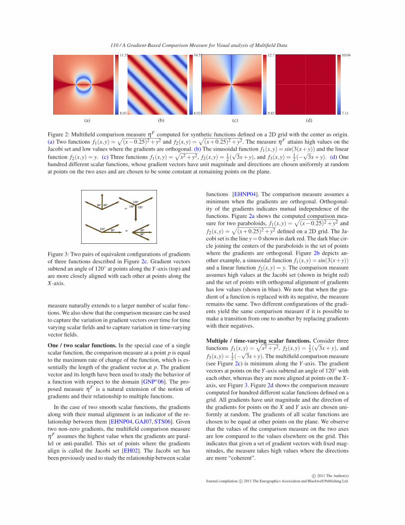
Figure 2: Multifield comparison measure ηF computed for synthetic functions defined on a 2D grid with the center as origin.(a) Two functions f1(x,y) =

√

(x−0.25)2 + y2 and f2(x,y) =√

(x+0.25)2 + y2. The measure ηF attains high values on theJacobi set and low values where the gradients are orthogonal. (b) The sinusoidal function f1(x,y) = sin(3(x+y)) and the linear

function f2(x,y) = y. (c) Three functions f1(x,y) =√

x2 + y2, f2(x,y) = 12 (√

3x + y), and f3(x,y) = 12 (−

√3x + y). (d) One

hundred different scalar functions, whose gradient vectors have unit magnitude and directions are chosen uniformly at randomat points on the two axes and are chosen to be some constant at remaining points on the plane.

=

=

Figure 3: Two pairs of equivalent configurations of gradientsof three functions described in Figure 2c. Gradient vectorssubtend an angle of 120◦ at points along the Y -axis (top) andare more closely aligned with each other at points along theX-axis.

measure naturally extends to a larger number of scalar func-tions. We also show that the comparison measure can be usedto capture the variation in gradient vectors over time for timevarying scalar fields and to capture variation in time-varyingvector fields.

One / two scalar functions. In the special case of a singlescalar function, the comparison measure at a point p is equalto the maximum rate of change of the function, which is es-sentially the length of the gradient vector at p. The gradientvector and its length have been used to study the behavior ofa function with respect to the domain [GNP∗06]. The pro-posed measure ηF is a natural extension of the notion ofgradients and their relationship to multiple functions.

In the case of two smooth scalar functions, the gradientsalong with their mutual alignment is an indicator of the re-lationship between them [EHNP04, GAJ07, STS06]. Giventwo non-zero gradients, the multifield comparison measureηF assumes the highest value when the gradients are paral-lel or anti-parallel. This set of points where the gradientsalign is called the Jacobi set [EH02]. The Jacobi set hasbeen previously used to study the relationship between scalar

functions [EHNP04]. The comparison measure assumes aminimum when the gradients are orthogonal. Orthogonal-ity of the gradients indicates mutual independence of thefunctions. Figure 2a shows the computed comparison mea-sure for two paraboloids, f1(x,y) =

√

(x−0.25)2 + y2 and

f2(x,y) =√

(x+0.25)2 + y2 defined on a 2D grid. The Ja-cobi set is the line y = 0 shown in dark red. The dark blue cir-cle joining the centers of the paraboloids is the set of pointswhere the gradients are orthogonal. Figure 2b depicts an-other example, a sinusoidal function f1(x,y) = sin(3(x+y))and a linear function f2(x,y) = y. The comparison measureassumes high values at the Jacobi set (shown in bright red)and the set of points with orthogonal alignment of gradientshas low values (shown in blue). We note that when the gra-dient of a function is replaced with its negative, the measureremains the same. Two different configurations of the gradi-ents yield the same comparison measure if it is possible tomake a transition from one to another by replacing gradientswith their negatives.

Multiple / time-varying scalar functions. Consider threefunctions f1(x,y) =

√

x2 + y2, f2(x,y) = 12 (√

3x + y), and

f3(x,y) = 12 (−

√3x+y). The multifield comparison measure

(see Figure 2c) is minimum along the Y -axis. The gradientvectors at points on the Y -axis subtend an angle of 120◦ witheach other, whereas they are more aligned at points on the X-axis, see Figure 3. Figure 2d shows the comparison measurecomputed for hundred different scalar functions defined on agrid. All gradients have unit magnitude and the direction ofthe gradients for points on the X and Y axis are chosen uni-formly at random. The gradients of all scalar functions arechosen to be equal at other points on the plane. We observethat the values of the comparison measure on the two axesare low compared to the values elsewhere on the grid. Thisindicates that given a set of gradient vectors with fixed mag-nitudes, the measure takes high values where the directionsare more “coherent”.




Given a single time varying scalar field, we construct theset F of multiple scalar functions with one function corre-sponding to each time step. The multifield comparison mea-sure in this case measures the variation of the scalar func-tion over time. We extend the measure to compare multiplevector fields or analyze the variation in time-varying vectorfields by replacing each row in the derivative matrix dF(p)with the input vector at the point p.

5. Computation

Evaluating the multifield comparison measure at a point re-quires the solution to a maximization problem. In this sec-tion, we describe how this computation can be reduced tothe faster evaluation of the maximum eigenvalue of a posi-tive semi-definite matrix.

Maximum eigenvalue computation. From the definitionsof the multifield comparison measure and the norm of a ma-trix, we have

ηFp =

(

maxx∈Rn,‖x‖=1

xT (dF(p))T (dF(p))x

)12

.

We rewrite the matrix product (dF(p))T (dF(p)) as UT ΛU ,where U is an orthogonal matrix and Λ is a diagonal matrixconsisting of the eigenvalues of (dF(p))T (dF(p)) as entriesin its diagonal. This follows from the spectral theorem fromlinear algebra [HK71]:

ηFp =

(

maxx∈Rn,‖x‖=1

xTUT ΛUx

)12

.

Since the orthogonal matrix U represents a length preserv-ing and invertible transformation, we can write the aboveexpression as

ηFp =

(

maxx∈Rn,‖x‖=1

xT Λx

)12

= max{√

λ : λ is a diagonal element of Λ}= max{

√λ : λ is an eigenvalue of (dF(p))T (dF(p))}.

For piecewise linear functions defined on a triangle mesh,the derivative matrix dF(p) is constant within a triangle andcan be computed by choosing a local coordinate system.When the data is available over a structured grid and lin-early interpolated along each coordinate axis, the differencebetween neighboring points in each axis direction can beused to approximate the partial derivatives at sample pointsand hence compute ηF . We note that following an approachsimilar to proving stability for piecewise linear functions, wecan show that the comparison measure computed using thisapproximation for the gradient is also robust to noise in theinput.

Analysis. The size of the n×n matrix (dF(p))T (dF(p)) de-pends only on the dimension of the domain. Therefore, thetime taken for computing the measure also depends only on

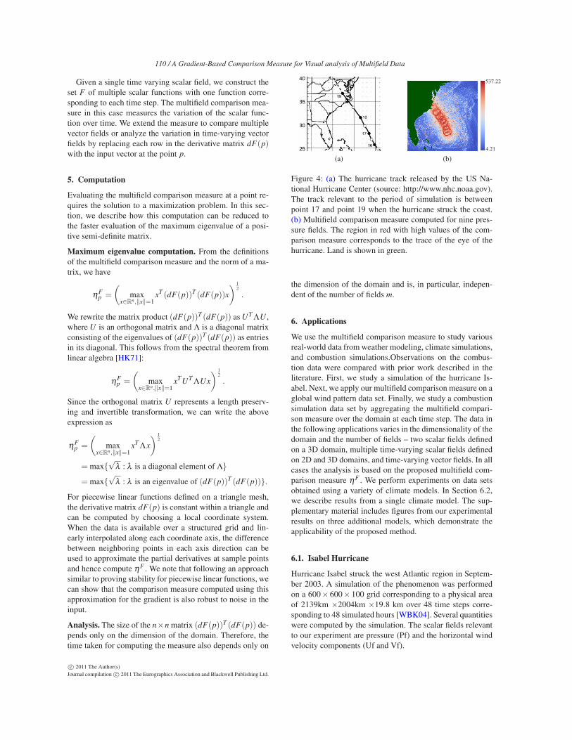
(a)

4.21

537.22

(b)

Figure 4: (a) The hurricane track released by the US Na-tional Hurricane Center (source: http://www.nhc.noaa.gov).The track relevant to the period of simulation is betweenpoint 17 and point 19 when the hurricane struck the coast.(b) Multifield comparison measure computed for nine pres-sure fields. The region in red with high values of the com-parison measure corresponds to the trace of the eye of thehurricane. Land is shown in green.

the dimension of the domain and is, in particular, indepen-dent of the number of fields m.

6. Applications

We use the multifield comparison measure to study variousreal-world data from weather modeling, climate simulations,and combustion simulations.Observations on the combus-tion data were compared with prior work described in theliterature. First, we study a simulation of the hurricane Is-abel. Next, we apply our multifield comparison measure on aglobal wind pattern data set. Finally, we study a combustionsimulation data set by aggregating the multifield compari-son measure over the domain at each time step. The data inthe following applications varies in the dimensionality of thedomain and the number of fields – two scalar fields definedon a 3D domain, multiple time-varying scalar fields definedon 2D and 3D domains, and time-varying vector fields. In allcases the analysis is based on the proposed multifield com-parison measure ηF . We perform experiments on data setsobtained using a variety of climate models. In Section 6.2,we describe results from a single climate model. The sup-plementary material includes figures from our experimentalresults on three additional models, which demonstrate theapplicability of the proposed method.

6.1. Isabel Hurricane

Hurricane Isabel struck the west Atlantic region in Septem-ber 2003. A simulation of the phenomenon was performedon a 600× 600× 100 grid corresponding to a physical areaof 2139km ×2004km ×19.8 km over 48 time steps corre-sponding to 48 simulated hours [WBK04]. Several quantitieswere computed by the simulation. The scalar fields relevantto our experiment are pressure (Pf) and the horizontal windvelocity components (Uf and Vf).




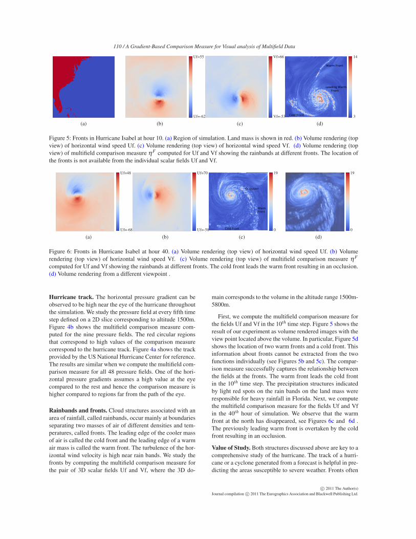
(a)

Uf=-62

Uf=55

(b)

Vf=-53

Vf=66

(c)

Warm Front

Leading Warm

Front

Cold Front 3

14

(d)

Figure 5: Fronts in Hurricane Isabel at hour 10. (a) Region of simulation. Land mass is shown in red. (b) Volume rendering (topview) of horizontal wind speed Uf. (c) Volume rendering (top view) of horizontal wind speed Vf. (d) Volume rendering (topview) of multifield comparison measure ηF computed for Uf and Vf showing the rainbands at different fronts. The location ofthe fronts is not available from the individual scalar fields Uf and Vf.

Uf=-68

Uf=48

(a)

Uf=-58

Uf=70

(b)

Cold Front

Occlusion

Warm

Front

0

19

(c)

0

19

(d)

Figure 6: Fronts in Hurricane Isabel at hour 40. (a) Volume rendering (top view) of horizontal wind speed Uf. (b) Volumerendering (top view) of horizontal wind speed Vf. (c) Volume rendering (top view) of multifield comparison measure ηF

computed for Uf and Vf showing the rainbands at different fronts. The cold front leads the warm front resulting in an occlusion.(d) Volume rendering from a different viewpoint .

Hurricane track. The horizontal pressure gradient can beobserved to be high near the eye of the hurricane throughoutthe simulation. We study the pressure field at every fifth timestep defined on a 2D slice corresponding to altitude 1500m.Figure 4b shows the multifield comparison measure com-puted for the nine pressure fields. The red circular regionsthat correspond to high values of the comparison measurecorrespond to the hurricane track. Figure 4a shows the trackprovided by the US National Hurricane Center for reference.The results are similar when we compute the multifield com-parison measure for all 48 pressure fields. One of the hori-zontal pressure gradients assumes a high value at the eyecompared to the rest and hence the comparison measure ishigher compared to regions far from the path of the eye.

Rainbands and fronts. Cloud structures associated with anarea of rainfall, called rainbands, occur mainly at boundariesseparating two masses of air of different densities and tem-peratures, called fronts. The leading edge of the cooler massof air is called the cold front and the leading edge of a warmair mass is called the warm front. The turbulence of the hor-izontal wind velocity is high near rain bands. We study thefronts by computing the multifield comparison measure forthe pair of 3D scalar fields Uf and Vf, where the 3D do-

main corresponds to the volume in the altitude range 1500m-5800m.

First, we compute the multifield comparison measure forthe fields Uf and Vf in the 10th time step. Figure 5 shows theresult of our experiment as volume rendered images with theview point located above the volume. In particular, Figure 5dshows the location of two warm fronts and a cold front. Thisinformation about fronts cannot be extracted from the twofunctions individually (see Figures 5b and 5c). The compar-ison measure successfully captures the relationship betweenthe fields at the fronts. The warm front leads the cold frontin the 10th time step. The precipitation structures indicatedby light red spots on the rain bands on the land mass wereresponsible for heavy rainfall in Florida. Next, we computethe multifield comparison measure for the fields Uf and Vfin the 40th hour of simulation. We observe that the warmfront at the north has disappeared, see Figures 6c and 6d .The previously leading warm front is overtaken by the coldfront resulting in an occlusion.

Value of Study. Both structures discussed above are key to acomprehensive study of the hurricane. The track of a hurri-cane or a cyclone generated from a forecast is helpful in pre-dicting the areas susceptible to severe weather. Fronts often




give valuable information about severe weather to the fore-caster. Rainbands at cold fronts are often strong in natureand can be responsible for heavy thunder storms. Typically,occlusion fronts are associated with thunder storms and theirpassage results in the reduction of humidity.

6.2. Global Wind Patterns

Prevailing winds are winds that blow in a dominant direc-tion at a particular point. Movements in the Earth’s atmo-sphere affect these winds. In regions of mid-latitudes, thewinds blow from west to the east and are known as west-erlies. The winds found in the tropics near the equator areeasterlies or trade winds. Figure 7a shows the different pre-vailing winds on earth. We study wind patterns on earthusing a climate simulation of 50 years between 1960 and2009 [RBB∗03]. The data is available for 600 time stepscorresponding to each month over the period of simulation.Each time step is a 3D grid with resolution corresponding to1◦×1◦×16plev (pressure elevations) on earth. Pressure el-evations correspond to pressures varying from 1000 hPa onthe surface to 30 hPa in the upper atmosphere.

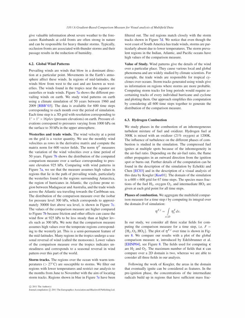
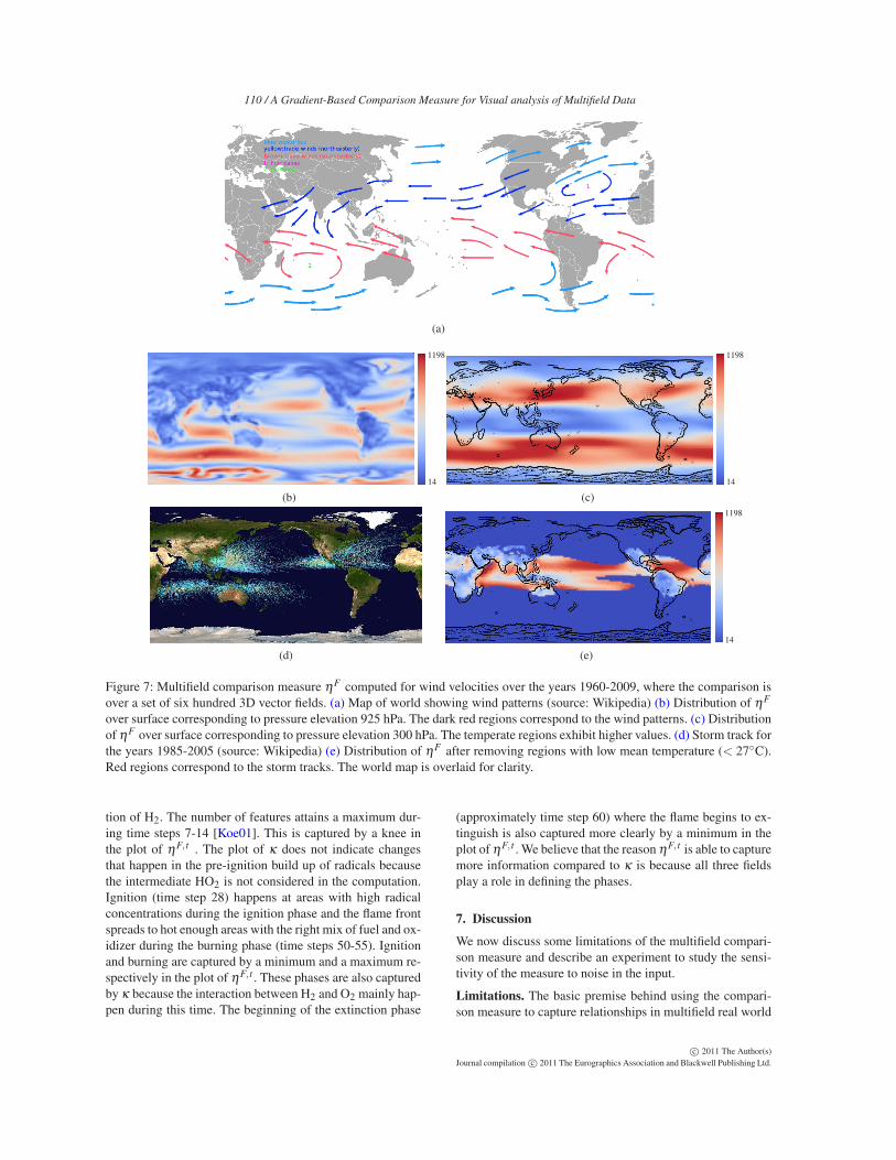
Westerlies and trade winds. The wind velocity at a pointon the grid is a vector quantity. We use the monthly windvelocities as rows in the derivative matrix and compute thematrix norm for 600 vector fields. The norm ηF measuresthe variation of the wind velocities over a time period of50 years. Figure 7b shows the distribution of the computedcomparison measure over a surface corresponding to pres-sure elevation 925 hPa. Comparing with wind patterns inFigure 7a, we see that the measure assumes high values inregions that lie in the path of prevailing winds, particularlythe westerlies found in the regions surrounding Antarctica,the region of hurricanes in Atlantic, the cyclone prone re-gion between Madagascar and Australia, and the trade windsacross the Atlantic sea traveling towards the Caribbean sea.The distribution of the comparison measure over the isobarfor pressure level 300 hPa, which corresponds to approxi-mately 30000 feet above sea level, is shown in Figure 7c.The values of the comparison measure are higher comparedto Figure 7b because friction and other effects can cause thewind flow at 925 hPa to be less steady than at higher lev-els such as 300 hPa. We note that the comparison measureassumes high values over the temperate regions correspond-ing to the westerly jet. This is a semi-permanent feature ofthe mid-latitudes. Many regions in the tropics undergo a sea-sonal reversal of wind (called the monsoons). Lower valuesof the comparison measure over the tropics indicates un-steadiness and corresponds to a seasonal reversal in windpattern over this part of the world.

Storm tracks. The regions over the ocean with warm tem-peratures (> 27◦C) are susceptible to storms. We filter outregions with lower temperatures and restrict our analysis tothe months from June to November with the aim of locatingstorm tracks. Regions shown in blue in Figure 7e have been

filtered out. The red regions match closely with the stormtracks shown in Figure 7d. We notice that even though thewest coast of South America has trade winds, storms are par-ticularly absent due to lower temperatures. The storm preva-lent regions in the Indian, Atlantic, and Pacific oceans havehigh values of the comparison measure.

Value of Study. Wind patterns give the details of the windover a particular place. They cause various local and globalphenomena and are widely studied by climate scientists. Forexample, the trade winds are responsible for tropical cy-clones over oceans. Storm tracks generated using winds giveus information on regions where storms are more probable.Computing storm tracks for long periods would require as-certaining tracks of every individual hurricane and cycloneand plotting them. Our approach simplifies this computationby considering all 600 time steps together to generate thedistribution of the comparison measure.

6.3. Hydrogen Combustion

We study phases in the combustion of an inhomogeneousturbulent mixture of fuel and oxidizer. Hydrogen fuel at300K is mixed with an oxidizer (21% oxygen) at 1200K.The influence of turbulence on the different phases of com-bustion is studied in the simulation. The compressed fuelignites at multiple spots because of the inhomogeneity inthe air-fuel ratio. Depending on the air-fuel ratio, the flameeither propagates in an outward direction from the ignitionspot or burns out. Further details of the computation can befound in the description of the simulation by Echekki andChen [EC03] and in the description of a visual analysis ofthis data by Koegler [Koe01]. The domain of the simulationis a 600×600 grid for 67 time steps. The species mass frac-tions of the fuel H2, oxygen O2, and intermediate HO2 aregiven at each grid point for all time steps.

Phases of combustion. We aggregate the multifield compar-ison measure for a time step t by computing its integral overthe domain D of simulation:

ηF, t =∫

x∈D

ηFx dx.

In our study, we consider all three scalar fields for com-puting the comparison measure for a time step, i.e. F ={H2,O2,HO2}. The plot of ηF, t over time is shown in Fig-ure 8. We compare our results with a plot of the globalcomparison measure κ , introduced by Edelsbrunner et al.[EHNP04], see Figure 8. The fields used for computing κare H2 and O2. The maximum number of fields that κ cancompare over a 2D domain is two, whereas we are able toconsider all three fields in our analysis.

Following the work of Koegler, the areas in the domainthat eventually ignite can be considered as features. In thepre-ignition phase, the concentrations of the intermediateradicals build up in regions that have sufficient mass frac-




(a)

14

1198

(b)

14

1198

(c)

(d)

14

1198

(e)

Figure 7: Multifield comparison measure ηF computed for wind velocities over the years 1960-2009, where the comparison isover a set of six hundred 3D vector fields. (a) Map of world showing wind patterns (source: Wikipedia) (b) Distribution of ηF

over surface corresponding to pressure elevation 925 hPa. The dark red regions correspond to the wind patterns. (c) Distributionof ηF over surface corresponding to pressure elevation 300 hPa. The temperate regions exhibit higher values. (d) Storm track forthe years 1985-2005 (source: Wikipedia) (e) Distribution of ηF after removing regions with low mean temperature (< 27◦C).Red regions correspond to the storm tracks. The world map is overlaid for clarity.

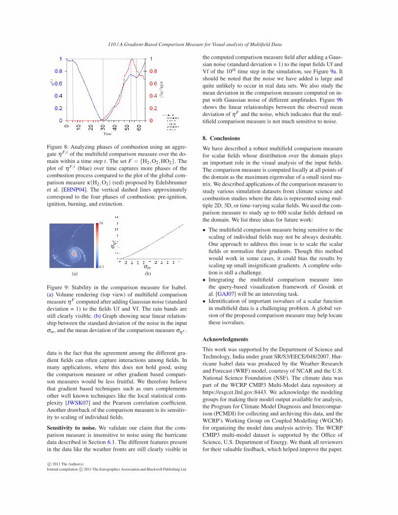
tion of H2. The number of features attains a maximum dur-ing time steps 7-14 [Koe01]. This is captured by a knee inthe plot of ηF, t . The plot of κ does not indicate changesthat happen in the pre-ignition build up of radicals becausethe intermediate HO2 is not considered in the computation.Ignition (time step 28) happens at areas with high radicalconcentrations during the ignition phase and the flame frontspreads to hot enough areas with the right mix of fuel and ox-idizer during the burning phase (time steps 50-55). Ignitionand burning are captured by a minimum and a maximum re-spectively in the plot of ηF, t . These phases are also capturedby κ because the interaction between H2 and O2 mainly hap-pen during this time. The beginning of the extinction phase

(approximately time step 60) where the flame begins to ex-tinguish is also captured more clearly by a minimum in theplot of ηF, t . We believe that the reason ηF, t is able to capturemore information compared to κ is because all three fieldsplay a role in defining the phases.

7. Discussion

We now discuss some limitations of the multifield compari-son measure and describe an experiment to study the sensi-tivity of the measure to noise in the input.

Limitations. The basic premise behind using the compari-son measure to capture relationships in multifield real world




Time

ηF,t κ

(H2,O

2 )

Figure 8: Analyzing phases of combustion using an aggre-gate ηF, t of the multifield comparison measure over the do-main within a time step t. The set F = {H2,O2,HO2}. Theplot of ηF, t (blue) over time captures more phases of thecombustion process compared to the plot of the global com-parison measure κ(H2,O2) (red) proposed by Edelsbrunneret al. [EHNP04]. The vertical dashed lines approximatelycorrespond to the four phases of combustion: pre-ignition,ignition, burning, and extinction.

0.1

16

(a)

σin

ση

F

(b)

Figure 9: Stability in the comparison measure for Isabel.(a) Volume rendering (top view) of multifield comparisonmeasure ηF computed after adding Gaussian noise (standarddeviation = 1) to the fields Uf and Vf. The rain bands arestill clearly visible. (b) Graph showing near linear relation-ship between the standard deviation of the noise in the inputσin, and the mean deviation of the comparison measure σηF .

data is the fact that the agreement among the different gra-dient fields can often capture interactions among fields. Inmany applications, where this does not hold good, usingthe comparison measure or other gradient based compari-son measures would be less fruitful. We therefore believethat gradient based techniques such as ours complementsother well known techniques like the local statistical com-plexity [JWSK07] and the Pearson correlation coefficient.Another drawback of the comparison measure is its sensitiv-ity to scaling of individual fields.

Sensitivity to noise. We validate our claim that the com-parison measure is insensitive to noise using the hurricanedata described in Section 6.1. The different features presentin the data like the weather fronts are still clearly visible in

the computed comparison measure field after adding a Gaus-sian noise (standard deviation = 1) to the input fields Uf andVf of the 10th time step in the simulation, see Figure 9a. Itshould be noted that the noise we have added is large andquite unlikely to occur in real data sets. We also study themean deviation in the comparison measure computed on in-put with Gaussian noise of different amplitudes. Figure 9bshows the linear relationships between the observed meandeviation of ηF and the noise, which indicates that the mul-tifield comparison measure is not much sensitive to noise.

8. Conclusions

We have described a robust multifield comparison measurefor scalar fields whose distribution over the domain playsan important role in the visual analysis of the input fields.The comparison measure is computed locally at all points ofthe domain as the maximum eigenvalue of a small sized ma-trix. We described applications of the comparison measure tostudy various simulation datasets from climate science andcombustion studies where the data is represented using mul-tiple 2D, 3D, or time-varying scalar fields. We used the com-parison measure to study up to 600 scalar fields defined onthe domain. We list three ideas for future work:

• The multifield comparison measure being sensitive to thescaling of individual fields may not be always desirable.One approach to address this issue is to scale the scalarfields or normalize their gradients. Though this methodwould work in some cases, it could bias the results byscaling up small insignificant gradients. A complete solu-tion is still a challenge.

• Integrating the multifield comparison measure intothe query-based visualization framework of Gosink etal. [GAJ07] will be an interesting task.

• Identification of important isovalues of a scalar functionin multifield data is a challenging problem. A global ver-sion of the proposed comparison measure may help locatethese isovalues.

Acknowledgments

This work was supported by the Department of Science andTechnology, India under grant SR/S3/EECE/048/2007. Hur-ricane Isabel data was produced by the Weather Researchand Forecast (WRF) model, courtesy of NCAR and the U.S.National Science Foundation (NSF). The climate data waspart of the WCRP CMIP3 Multi-Model data repository athttps://esgcet.llnl.gov:8443. We acknowledge the modelinggroups for making their model output available for analysis,the Program for Climate Model Diagnosis and Intercompar-ison (PCMDI) for collecting and archiving this data, and theWCRP’s Working Group on Coupled Modelling (WGCM)for organizing the model data analysis activity. The WCRPCMIP3 multi-model dataset is supported by the Office ofScience, U.S. Department of Energy. We thank all reviewersfor their valuable feedback, which helped improve the paper.




References

[BPRS98] BAJAJ C., PASCUCCI V., RABBIOLO G., SCHIKORE

D.: Hypervolume visualization: a challenge in simplicity. InProc. IEEE Symp. Volume Visualization (1998), pp. 95–102. 2

[BW08] BACHTHALER S., WEISKOPF D.: Continuous scatter-plots. IEEE Transactions on Visualization and Computer Graph-

ics 14, 6 (2008), 1428–1435. 2

[CS99] CAI W., SAKAS G.: Data intermixing and multi-volumerendering. Computer Graphics Forum 18, 3 (1999), 359–368. 2

[CSA00] CARR H., SNOEYINK J., AXEN U.: Computing con-tour trees in all dimensions. In Proc. ACM-SIAM Symposium on

Discrete algorithms (2000), pp. 918–926. 1

[CSvdP04] CARR H., SNOEYINK J., VAN DE PANNE M.: Sim-plifying flexible isosurfaces using local geometric measures. InProc. IEEE Conf. Visualization (2004), pp. 497–504. 1

[EC03] ECHEKKI T., CHEN J. H.: Direct numerical simulationof autoignition in nonhomogeneous hydrogen-air mixtures. Com-

bustion and Flame 134, 3 (2003), 169–191. 7

[EH02] EDELSBRUNNER H., HARER J.: Jacobi set of multiplemorse funtions. In Foundations of Computational Mathematics,

Minneapolis (2002), Cambridge Univ. Press, pp. 37–57. 4

[EHNP04] EDELSBRUNNER H., HARER J., NATARAJAN V.,PASCUCCI V.: Local and global comparison of continuous func-tions. In Proc. IEEE Conf. Visualization (2004), pp. 275–280. 2,4, 7, 9

[GAJ07] GOSINK L., ANDERSON J. BETHEL W., JOY K.: Vari-able interactions in query-driven visualization. IEEE Transac-

tions on Visualization and Computer Graphics 13, 6 (2007),1400–1407. 2, 4, 9

[GNP∗06] GYULASSY A., NATARAJAN V., PASCUCCI V., BRE-MER P.-T., HAMANN B.: A topological approach to simplifica-tion of three-dimensional scalar functions. IEEE Transactions on

Visualization and Computer Graphics 12, 4 (2006), 474–484. 4

[HJ85] HORN R., JOHNSON C.: Matrix Analysis. CambridgeUniversity Press, 1985. 2

[HJ04] HANSEN C., JOHNSON C.: Visualization Handbook.Academic Press, 2004. 1

[HK71] HOFFMAN K., KUNZE R.: Linear Algebra. PrenticeHall, 1971. 5

[JBTS08] JÄNICKE H., BOTTINGER M., TRICOCHE X.,SCHEUERMANN G.: Automatic detection and visualization ofdistinctive structures in 3d unsteady multi-fields. Computer

Graphics Forum 27, 3 (2008), 767–774. 2

[JWSK07] JÄNICKE H., WIEBEL A., SCHEUERMANN G.,KOLLMANN W.: Multifield visualization using local statisticalcomplexity. IEEE Transactions on Visualization and Computer

Graphics 13 (2007), 1384–1391. 2, 9

[Koe01] KOEGLER W. S.: Case study: application of featuretracking to analysis of autoignition simulation data. In Proc.

IEEE Conf. Visualization (2001), pp. 461–464. 7, 8

[LS09] LEE T.-Y., SHEN H.-W.: Visualization and explorationof temporal trend relationships in multivariate time-varying data.IEEE Transactions on Visualization and Computer Graphics 15

(2009), 1359–1366. 2

[NN10] NAGARAJ S., NATARAJAN V.: Relation-awareisosurface extraction in multi-field data. IEEE Trans-

actions on Visualization and Computer Graphics (2010).http://doi.ieeecomputersociety.org/10.1109/TVCG.2010.64. 2

[PWH01] PEKAR V., WIEMKER R., HEMPEL D.: Fast detectionof meaningful isosurfaces for volume data visualization. In Proc.

IEEE Conf. Visualization (2001), pp. 223–230. 1

[RBB∗03] ROECKNER E., BÄUML G., BONAVENTURA L.,BROKOPF R., ESCH M., GIORGETTA M., HAGEMANN S.,KIRCHNER I., KORNBLUEH L., MANZINI E., RHODIN A.,SCHLESE U., SCHULZWEIDA U., TOMPKINS A.: The Atmo-

spheric General Circulation Model ECHAM5. PART 1: Model

Description. Tech. Rep. 349, Max Planck Institute of Meteorol-ogy, 2003. 7

[SML06] SCHROEDER W., MARTIN K., LORENSEN B.: The Vi-

sualization Toolkit An Object-Oriented Approach To 3D Graph-

ics, 4th Edition. Kitware, Inc., 2006. 1

[STS06] SAUBER N., THEISEL H., SEIDEL H.-P.: Multifield-graphs: An approach to visualizing correlations in multifieldscalar data. IEEE Transactions on Visualization and Computer

Graphics 12, 5 (2006), 917–924. 2, 4

[WBK04] WANG W., BRUYERE C., KUO B.: Competition dataset and description in 2004 IEEE Visualization design contest,2004. http://vis.computer.org/vis2004contest/data.html. 5

[WS06] WOODRING J., SHEN H.-W.: Multi-variate, time vary-ing, and comparative visualization with contextual cues. IEEE

Transactions on Visualization and Computer Graphics 12, 5(2006), 909–916. 2



A Gradient-Based Comparison Measure for Visual...

Documents

Transcript of A Gradient-Based Comparison Measure for Visual...