University of Tennessee, Knoxville University of Tennessee, Knoxville

TRACE: Tennessee Research and Creative TRACE: Tennessee Research and Creative

Exchange Exchange

Masters Theses Graduate School

8-2017

A GPU Implementation of Distance-Driven Computed Tomography A GPU Implementation of Distance-Driven Computed Tomography

Ryan D. Wagner University of Tennessee, Knoxville, rfx468@vols.utk.edu

Follow this and additional works at: https://trace.tennessee.edu/utk_gradthes

Part of the Numerical Analysis and Scientific Computing Commons, Other Computer Sciences

Commons, Software Engineering Commons, and the Theory and Algorithms Commons

Recommended Citation Recommended Citation Wagner, Ryan D., "A GPU Implementation of Distance-Driven Computed Tomography. " Master's Thesis, University of Tennessee, 2017. https://trace.tennessee.edu/utk_gradthes/4909

This Thesis is brought to you for free and open access by the Graduate School at TRACE: Tennessee Research and Creative Exchange. It has been accepted for inclusion in Masters Theses by an authorized administrator of TRACE: Tennessee Research and Creative Exchange. For more information, please contact trace@utk.edu.

To the Graduate Council:

I am submitting herewith a thesis written by Ryan D. Wagner entitled "A GPU Implementation of

Distance-Driven Computed Tomography." I have examined the final electronic copy of this thesis

for form and content and recommend that it be accepted in partial fulfillment of the

requirements for the degree of Master of Science, with a major in Computer Science.

Jens Gregor, Major Professor

We have read this thesis and recommend its acceptance:

Gregory D. Peterson, Stanimire Tomov

Accepted for the Council:

Dixie L. Thompson

Vice Provost and Dean of the Graduate School

(Original signatures are on file with official student records.)

A GPU Implementation of

Distance-Driven Computed

Tomography

A Thesis Presented for the

Master of Science

Degree

The University of Tennessee, Knoxville

Ryan D. Wagner

August 2017

c© by Ryan D. Wagner, 2017

All Rights Reserved.

ii

Acknowledgements

I would like to thank my thesis advisor, Jens Gregor, as well as Thomas Benson of

Morpho Detection, LLC for their advising and instruction throughout this process.

Thank you to Elizabeth Wagner nee Carter for editing this document for publication.

I would also like to thank my thesis committee, including Jens Gregor, Gregory

Peterson, and Stanimire Tomov. Finally, I would like to thank Morpho Detection

LLC for funding my work.

iii

Abstract

Computed tomography (CT) is used to produce cross-sectional images of an

object via noninvasive X-ray scanning of the object. These images have a wide

range of uses including threat detection in checked baggage at airports. The

projection data collected by the CT scanner must be reconstructed before the

image may be viewed. In comparison to filtered backprojection methods of

reconstruction, iterative reconstruction algorithms have been shown to increase overall

image quality by incorporating a more complete model of the underlying physics.

Unfortunately, iterative algorithms are generally too slow to meet the high throughput

demands of this application. It is therefore worthwhile to investigate methods of

improving their execution time. This paper discusses multiple implementations of

iterative tomographic reconstruction using the simultaneous iterative reconstruction

technique (SIRT) and the distance-driven system model. The primary focus is an

implementation of the branchless variant of the distance-driven system model on a

graphics processing unit (GPU). Solutions to key implementation concerns which have

been neglected in previous literature are discussed.

iv

Table of Contents

1 Introduction 1

1.1 The Purposes and Uses of Computed Tomography . . . . . . . . . . . 1

1.2 Projection Data . . . . . . . . . . . . . . . . . . . . . . . . . . . . . . 2

1.3 Scanner Geometry . . . . . . . . . . . . . . . . . . . . . . . . . . . . 3

1.4 Reconstruction Methods . . . . . . . . . . . . . . . . . . . . . . . . . 5

1.5 System Models . . . . . . . . . . . . . . . . . . . . . . . . . . . . . . 6

1.6 GPU Implementation . . . . . . . . . . . . . . . . . . . . . . . . . . . 6

2 Iterative Reconstruction 8

2.1 The Simultaneous Iterative Reconstruction Technique . . . . . . . . . 8

2.2 SIRT Applied to Statistically Weighted Least Squares . . . . . . . . . 10

2.3 Image Convergence . . . . . . . . . . . . . . . . . . . . . . . . . . . . 10

3 System Models 13

3.1 General System Models . . . . . . . . . . . . . . . . . . . . . . . . . . 13

3.2 Distance-Driven System Model . . . . . . . . . . . . . . . . . . . . . 14

3.2.1 Distance-Driven in Two-Dimensions . . . . . . . . . . . . . . . 15

3.2.2 Distance-Driven in Three-Dimensions . . . . . . . . . . . . . . 17

3.2.3 Distance-Driven Branchless Modification . . . . . . . . . . . . 18

4 Implementation 22

4.1 Naive Branched Implementations . . . . . . . . . . . . . . . . . . . . 22

v

4.2 Branched Implementation . . . . . . . . . . . . . . . . . . . . . . . . 23

4.3 Branchless Implementations . . . . . . . . . . . . . . . . . . . . . . . 25

4.3.1 Computation of Integral Image and Integral Rays . . . . . . . 26

5 Results and Discussion 30

5.1 Performance Comparison . . . . . . . . . . . . . . . . . . . . . . . . . 30

5.2 Potential Performance Improvements . . . . . . . . . . . . . . . . . . 33

5.3 Image Quality . . . . . . . . . . . . . . . . . . . . . . . . . . . . . . . 34

5.3.1 Floating-Point Precision . . . . . . . . . . . . . . . . . . . . . 34

5.3.2 Texture Interpolation . . . . . . . . . . . . . . . . . . . . . . . 34

5.3.3 Border Elements . . . . . . . . . . . . . . . . . . . . . . . . . 35

5.3.4 Ray Value Leakage . . . . . . . . . . . . . . . . . . . . . . . . 37

5.3.5 Reconstructed Images . . . . . . . . . . . . . . . . . . . . . . 38

6 Conclusion 41

Bibliography 43

Vita 47

vi

List of Figures

1.1 A selection of source and detector arrangements. . . . . . . . . . . . . 3

1.2 The coordinate system and geometry. . . . . . . . . . . . . . . . . . . 4

2.1 The average weighted projection data error of an image quality bag

reconstruction over 23 iterations. . . . . . . . . . . . . . . . . . . . . 11

2.2 Reconstructed image quality bag after various iterations . . . . . . . 12

3.1 Illustration of the line intersection model . . . . . . . . . . . . . . . . 14

3.2 Illustration of a voxel-driven method . . . . . . . . . . . . . . . . . . 15

3.3 Voxel and detector mappings at different rotation angles . . . . . . . 16

3.4 Rectangular sum computation . . . . . . . . . . . . . . . . . . . . . . 18

3.5 Integral image summation where all voxel values and areas are 1 . . . 19

3.6 Computation of an image plane’s contribution to a ray value . . . . . 19

3.7 Mapping of detector array to common plane . . . . . . . . . . . . . . 21

4.1 Code excerpt for computation of weighted row overlap . . . . . . . . 24

4.2 Code excerpt for computation of weighted column overlap . . . . . . 25

4.3 Interpolation from mapped detector elements to a uniform grid . . . . 28

5.1 Comparison of single iteration reconstruction time . . . . . . . . . . . 31

5.2 Speedup of single iteration reconstruction time . . . . . . . . . . . . . 32

5.3 Comparison of row sum values produced with various voxel size to

detector size ratios . . . . . . . . . . . . . . . . . . . . . . . . . . . . 35

5.4 Forward projection output with and without border voxels . . . . . . 36

vii

5.5 Illustration of ray value leakage in the integral rays . . . . . . . . . . 38

5.6 The effects of ray value leakage . . . . . . . . . . . . . . . . . . . . . 38

5.7 Artifacts resulting from ray value leakage . . . . . . . . . . . . . . . . 39

5.8 Reconstruction of image quality bag . . . . . . . . . . . . . . . . . . . 40

5.9 Reconstruction of resolution bag . . . . . . . . . . . . . . . . . . . . . 40

viii

Chapter 1

Introduction

1.1 The Purposes and Uses of Computed Tomog-

raphy

Computed tomography (CT) is primarily used in situations where tomographic, or

cross-sectional, views of an object are required and it is not possible to cut into

the object physically. CT scans are typically employed in medical settings to aid

in diagnostic medicine. Another application – most relevant to this thesis – is

the detection of security threats in checked airport luggage. CT scans allow for

automated or manual examination of luggage contents for hazardous materials or

other potentially dangerous items and are part of the last line of defense for preventing

these threats from being loaded onto an aircraft [1]. CT scanners are well suited for

this task due to their ability to create tomographic images, which can be used to

estimate density and volume of objects in the luggage. If the density and volume of

an object is suspect, it can be automatically flagged for further inspection [2].

1

1.2 Projection Data

The data used to create tomographic images is generated by passing X-rays through

the object of interest and detecting the rays on the other side of the object. As the

rays pass through the object, they are attenuated, or reduced in intensity, primarily

through the processes of photoabsorption and compton scattering. Different materials

have different coefficients of attenuation, and the longer an X-ray travels through a

material, the more it will be attenuated. Measuring the intensity of a ray which

has passed through an object and comparing it to the original intensity allows for

the computation of the attenuation and aids in determining its material makeup [3].

Multiple X-ray images, referred to in this paper as projections or views, are taken of

the object at different angles to generate the projection data. This projection data is

then processed to produce tomographic images.

By approximating the X-ray transmitted intensity as a monoenergetic beam, the

Beer-Lambert Law (1.1) can be used to determine the intensity I1 of radiation with

initial intensity I0 as it travels through an object with a spatially variant attenuation

coefficient µ dependent on coordinates x, y, and z along line, or ray, L:

I1 = I0e−

∫L µ(x,y,z)dl (1.1)

which can also be expressed as:

∫L

µ(x, y, z)dl = − logI1I0

(1.2)

By discretizing the object as an image grid of elements with individual attenuation

values, and with a discrete number of views and rays, this can be represented as a

linear system Ax = y, where

A ≡∫L

dl x ≡ µ(x, y, z) y ≡ − logI1I0

(1.3)

2

Note the projection data y is the negative log of the measured intensity divided by

the initial intensity. In practice, a blank scan with no object in the gantry is used

to represent the initial intensity. Later, this blank scan is used to log normalize the

projection data before reconstruction.

1.3 Scanner Geometry

System geometry describes the physical attributes and parameters of the CT scanner

used to generate the projection data. Early scanners used a parallel beam geometry

in which a single source and detector shift up and down before rotating to collect

data from multiple parallel beams; fan beam geometries use a single source and a

column of detectors; and cone beam geometries collect data in two-dimensions using

a single source and a 2D array of detectors. Detector arrays are generally either flat or

curved panel arrays. Flat panel detector arrays have equidistant columns of detectors

and curved panel detector arrays have equiangular detector columns. 2D images are

generated by scanners with a single column of detectors, and 3D images are typically

generated by scanners with a 2D array of detectors [4]. Figure 1.1 shows examples of

parallel, fan, and cone beam geometries.

Equiangular Fan BeamEquidistant Fan BeamParallel Beam Equiangular Cone Beam

Figure 1.1: A selection of source and detector arrangements.

When a 3D object is longer than the width of the detector array, a helical scan is

performed by adding a pitch to the detector and source rotation. The development

of helical scanners was motivated by the desire to scan an entire human organ in

3

a single breath. Cone beam helical scanners were later developed to improve the

isotropic spatial resolution [5]. Figure 1.2 shows the coordinate system and geometry

used in this research. Note the luggage being scanned moves down the gantry in the

positive z direction.

+x

+y

+zvoxel index(0,0,0)

source

+x

+y

0◦

90◦

180◦

270◦

depth

column

row

Detector Array

Helical Pathof source

and detectors

voxel index(row, column, depth)

+z

Figure 1.2: The coordinate system and geometry.

The system geometry used in this research is as follows:

• Helical, cone beam scanner

• 120mm pitch

• Equiangular detector array of 720 detector rows and 56 detector columns

• 2mm x 2mm detector pixels

• 1000 projections per rotation with 5 rotations

• 1500mm source to detector distance

• 900mm source to isocenter distance

• Translation in the z direction

The projection data used for reconstruction was provided via simulation by

Morpho Detection LLC and consists of two separate data sets. The first is a bag used

4

to test image quality. Notable contents include a water cylinder, scatter phantom

(delrin block), aluminum bar, teflon bar, and a string of metal spheres. The second

bag is designed to test resolution and penetration. It includes a block with resolution

bars and a second with thin wires. It also contains a highly attenuating lead block.

1.4 Reconstruction Methods

Image reconstruction techniques are generally divided into analytic and iterative

methods. The analytic methods, such as filtered back-projection, approximate the

solution using a closed form equation [5]. The iterative methods take either an

algebraic approach to solve for the solution to the linear system as described in

§1.2, or a statistical approach which maximizes a likelihood of the measurements

[6]. The analytic methods are the most commonly used in commercial settings,

primarily because closed form solutions are more computationally efficient than

iterative methods [2, 5]. Despite the difference in overall reconstruction time, iterative

reconstruction methods are preferable in some situations because of their potential

to improve image quality by incorporating a more complete model of the underlying

physics. Iterative methods are able to produce better images when working with

incomplete data, such as limited view angles or opaque objects in the field of view [7,

8]. Thibault et al. showed that iterative methods can also be used to provide more

accurate noise and complex geometry modeling as well as higher image resolution

and reduced helical artifacts [9]. Due to these image quality advantages of iterative

methods, it is desirable to investigate ways of increasing their reconstruction speed.

Chapter 2 describes the simultaneous iterative reconstruction technique which is the

reconstruction method used in this research. Other reconstruction algorithms could

be easily substituted, and the algorithm itself is not the focus of this work.

5

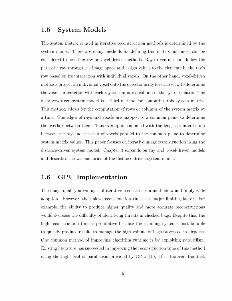
1.5 System Models

The system matrix A used in iterative reconstruction methods is determined by the

system model. There are many methods for defining this matrix and most can be

considered to be either ray or voxel-driven methods. Ray-driven methods follow the

path of a ray through the image space and assign values to the elements in the ray’s

row based on its interaction with individual voxels. On the other hand, voxel-driven

methods project an individual voxel onto the detector array for each view to determine

the voxel’s interaction with each ray to compute a column of the system matrix. The

distance-driven system model is a third method for computing this system matrix.

This method allows for the computation of rows or columns of the system matrix at

a time. The edges of rays and voxels are mapped to a common plane to determine

the overlap between them. This overlap is combined with the length of intersection

between the ray and the slab of voxels parallel to the common plane to determine

system matrix values. This paper focuses on iterative image reconstruction using the

distance-driven system model. Chapter 3 expands on ray and voxel-driven models

and describes the various forms of the distance-driven system model.

1.6 GPU Implementation

The image quality advantages of iterative reconstruction methods would imply wide

adoption. However, their slow reconstruction time is a major limiting factor. For

example, the ability to produce higher quality and more accurate reconstructions

would decrease the difficulty of identifying threats in checked bags. Despite this, the

high reconstruction time is prohibitive because the scanning systems must be able

to quickly produce results to manage the high volume of bags processed in airports.

One common method of improving algorithm runtime is by exploiting parallelism.

Existing literature has succeeded in improving the reconstruction time of this method

using the high level of parallelism provided by GPUs [10, 11]. However, this task

6

is not straightforward, and these papers provide few implementation details. This

research outlines some of the difficulties of implementation, provides a solution, and

discusses how future improvements could be made. Chapter 4 provides details on

the implementation of distance-driven image reconstruction, and Chapter 5 discusses

results and performance.

Cuda is an application programming interface created by NVIDIA for the

programming of NVIDIA GPUs using C [12]. Other languages such as C++ and

Fortran are also supported. When programming a GPU using Cuda, both the CPU

and GPU are used. The host refers to the CPU and main memory, while the device

refers to the GPU and its onboard memory. The host is capable of copying and

moving memory to and from the device and within the device itself. It is also able

to call functions known as kernels which execute on the device. In this way, it is

possible to interleave CPU and GPU computation. However, in the implementations

discussed here, the majority of the work is performed on the GPU after the host

copies all relevant data to the device.

The individual unit of execution in Cuda is a thread. Threads are grouped into

blocks and blocks are grouped into grids. Warps are groups of 32 threads within a

block that are created and executed together. Threads in a warp execute the same

instruction at the same time. However, if these threads reach a data-dependent

conditional branch, the two paths of the branch must be executed serially with the

threads not on the current path disabled.

In general, threads on a GPU execute more slowly than threads on a CPU.

However, significantly more threads can be executed at a time on a GPU than on

a CPU. Therefore, given a sufficiently parallel workload, a GPU will provide better

throughput.

7

Chapter 2

Iterative Reconstruction

As mentioned in §1.2, the relationship between the image and projection data can be

represented as a linear system. Because it is typical for there to be significantly more

rays than voxels, this system is expected to be overdetermined [4]. The result is that

this linear system cannot be solved directly [3]. Therefore, the goal is to compute an

approximation, x, of the scanned object.

2.1 The Simultaneous Iterative Reconstruction Tech-

nique

The simultaneous iterative reconstruction technique (SIRT) is one choice for solving

this linear system [4]:

x(k+1) = x(k) + αCATR(y − Ax(k)) (2.1)

The variable k represents the iteration. The initial image x(0) can take any value.

The closer it is to an accurate representation the object, the faster the iteration will

converge. It is possible to compute a less accurate approximation of the object to use

as x(0), such as by filtered backprojection; however, in this research all elements are

8

initialized to zero. The matrix C = diag{1/ci} is a diagonal preconditioning matrix

whose elements are inverse column sums ci of the system matrix A. Similarly, the

matrix R = diag{1/ri} is a diagonal matrix of inverse row sums ri. The vector y

is the log normalized projection data. The relaxation parameter α defines the step

size, and was shown to have an optimal value of 2/(1 + ε) ≈ 1.99 [13]. The operation

Ax(k) is the forward projection. It computes ray values based on the current image

approximation. The resulting ray values are then subtracted from the projection

data and weighted by the system matrix row sums to determine the error between the

observed and approximated projection data. The backprojection operation multiplies

the transpose of the system matrix and this projection data error and weights it by

the column sums to produce an update to the image approximation.

Let the weighted projection data error be e. Then, in 3D forward projection, the

weighted projection data error for a ray i is computed as:

e(k)i =

1

ri(yi −

∑j∈I

aijx(k)j ) (2.2)

where I is the set of all voxels. Let the u be the image update vector. Then the

update value for voxel j is computed as:

u(k)j =

1

cj

∑i∈D

aije(k)i (2.3)

where D is the set of all rays. Equation 2.1 can be rewritten as:

x(k+1) = x(k) + αu(k) (2.4)

9

2.2 SIRT Applied to Statistically Weighted Least

Squares

Though SIRT is an effective method of producing a reconstructed image, it can be

improved by the addition of statistical weighting. Sauer and Bouman showed that a

statistical model of the projections as Poisson-distributed random variables leads to

a weighted least squares problem x∗ = argmin(F (x)), where F (x) = 12||y − Ax||2W

[14]. The weight matrix W is a diagonal matrix of the variance associated with each

ray. Therefore, W = diag{λie−yi} where λi is the initial intensity of ray i. This

weighted least squares problem can be solved using preconditioned gradient descent

as x(k+1) = x(k) − αDOF (x(k)), where D is a preconditioning matrix. In comparison,

SIRT solves a geometrically weighted least squares problem x∗ = argmin(12||y −

Ax||2R)[6]. This R weighting is based on the amount of intersection between each

ray and the image and therefore, the more a ray intersects the image, the larger its

error tolerance [6]. In the case of noisy data, a statistical weighting is preferable.

Gregor and Fessler showed that SIRT can be modified to include this statistical

weighting via a variable transformation to solve the weighted least squares problem

using preconditioned gradient descent [6]. A is modified to be A = [aij] where aij =

wiriaij, and therefore, C is a diagonal matrix of inverse column sums of A and R is

a diagonal matrix of inverse row sums of A. The projection data y is modified to

be y = wiriyi. Then, this modified SIRT is given as x(k+1) = x(k) − αCOF (x(k)) =

x(k) +αCAT R(y− Ax(k)) and can be simplified to x(k+1) = x(k) +αCATW (y−Ax(k)).

2.3 Image Convergence

As the reconstruction algorithm iteratively improves the image approximation, the

average weighted projection data error decreases. This average error serves as a

good metric for the rate of convergence. Figure 2.1 shows this average error over

23 iterations of the image quality bag. Note the error decreases quickly for the

10

first few iterations as the major bag features start to form and slows down as the

details are improved. Given a sufficient number of iterations, the average error will

converge to a fixed value; however, complete convergence is not typically required and

reconstruction is terminated after a fixed number of iterations or once the average

error passes a threshold. Figure 2.2. shows the improvement of image quality for a

selection of iterations.

Figure 2.1: The average weighted projection data error of an image quality bagreconstruction over 23 iterations.

The rate of convergence can be increased through a method known as ordered

subsets [15]. Nearby rays are likely to contain similar or redundant information;

therefore, orthogonal rays are expected to provide the most new information. The

projection data is then divided into subsets which prioritize the distance between

rays in a subset and rays in subsequent subsets. An iteration of the reconstruction

algorithm is then divided into subiterations which update the image using only the

rays in the subset. Use of ordered subsets was not pursued in this work.

11

Figure 2.2: A slice though the image quality bag showing cross section of the teflonbar (left) and water bottle (right). Iterations shown are: 1, 2, 10, 20, 30, 57. Imagelookup table used is fire. Colors in order of increasing value are: blue, red, yellow,white.

12

Chapter 3

System Models

3.1 General System Models

Each row of the system matrix represents a projection ray and each column represents

an image voxel. Therefore, each element in A is a quantification of the voxel’s

potential to attenuate the ray. There are many system models, or methods for creating

this system matrix, and they are integral to the iterative reconstruction process. The

quality of the reconstructed image is dependent on the accuracy of the system matrix

[3]. Since the size of the system matrix is the number of projection data values

multiplied by the number of image voxels, it is typically too large to store in memory.

Instead, elements of the system matrix are computed as needed. This computation

accounts for a significant percentage of the overall reconstruction time; therefore, the

generation of the system matrix must balance accuracy and computational cost [3].

System models can typically be divided into two classes: ray or voxel-driven

methods. Ray-driven methods follow the path of a ray through the image and

calculate a row of the system matrix at a time. Voxel – or pixel in the 2D case – driven

methods iterate through the voxels and calculate a column of the system matrix at a

time [3]. An example of a ray-driven approach is the line intersection model (Fig. 3.1).

Rays are represented as a line drawn from the source to the center of a detector. The

13

value of an element ai,j in the system matrix corresponds to the length of intersection

between the ray i and the voxel j [3]. There are computationally efficient methods

for computing this model such as Siddon’s method [16] and an improved version by

Jacobs [17]. Unfortunately, the line intersection approach suffers from ring artifacts

for cone beam data due to the approximation of the volumetric x-ray beam as a line

[18]. A method which almost completely eliminates these ring artifacts at the cost

of additional computation, uses interpolation to assign support values: Interpolation

coefficients are determined for the nearest voxel centers at equally spaced points on the

ray. These coefficients then determine the support provided by the ray to those nearest

voxels [3]. An example of a simple voxel-driven approach computes system matrix

elements as follows (Fig. 3.2): for each projection, compute the coordinates of each

detector center; compute the line from the source through a voxel to the detector plane

and find the intersection point with the detector plane; use interpolation between

the intersection point and the values of the bounding detectors to compute their

approximate contribution [19].

Figure 3.1: Illustration of the line intersection model

3.2 Distance-Driven System Model

A system model which does not fit into ray or voxel-driven categories is the distance-

driven model, developed by De Man and Basu in 2003 [20]. The distance-driven

system model has similarities to both ray and voxel-driven methods and can compute

either system matrix rows or columns. This is in contrast to the ray-driven methods

which only compute system matrix rows and the voxel-driven methods which only

14

y

x

d1

d2

p

d3

d4

source

Figure 3.2: Illustration of a voxel-driven method

compute system matrix columns. This simplifies the parallelization of the distance-

driven method. It is possible to directly compute entire ray values during projection

and entire voxel values during backprojection instead of having to compute partial

values during ray-driven backprojection and voxel-driven forward projection.

3.2.1 Distance-Driven in Two-Dimensions

During forward and back projection in 2D, both the detectors and the pixels are

mapped to a common axis. The choice of common axis depends on how the rotation

of the scanner is represented in implementation. The mapping is done by determining

the line between the source and the point to be mapped then finding its intercept

with the common axis, as shown in Figure 3.3.

In a traditional case, the pixels are fixed relative to the coordinate system and the

source and detectors are rotated around the image. As a result, whichever axis is most

orthogonal to the current source rotation angle is chosen. When mapping to the x

axis, the pixel edges to the left and right are mapped, while when mapping the y axis

15

the top and bottom pixel edges are chosen (Fig. 3.3). This results in non-overlapping

pixel mapping within image slabs parallel to the common axis.

y

x

y

x

y

x

Figure 3.3: Pixel and detector mappings at different rotation angles. Left maps thecenter of the left and right pixel edges to the x axis. Center maps the center of thetop and bottom pixel edges to the y axis. Right shows that pixel mappings of imageslabs are uniform and non-overlapping.

The system matrix value for ray i and pixel j is:

aij =t

cosφ

oijwi

(3.1)

where t represents the width of the pixel in the dimension orthogonal to the common

axis, φ represents the angle between the ray and the axis orthogonal to the common

axis, oij represents the amount of overlap between the mapped pixel and detector,

and wi represents the width of the mapped detector. The component tcosφ

is known as

the slab intersection length. It is a measurement of the distance a ray travels through

a slab of pixels. In 2D, a slab of pixels is an image row when mapping to the x axis

and an image column when mapping to the y axis. The componentoijwi

represents

the fraction pixel j overlaps ray i. This calculation can be thought of intuitively

as follows: Each ray travels through an image slab for a distance given by the slab

intersection length. Because pixels in an image slab are non-overlapping and are

parallel to the common axis, they also map to the common axis in a non-overlapping

way. Therefore, each pixel in an image slab is assigned a fractional part of the slab

intersection length based on how much it overlaps with the ray.

16

It is also possible to fix the source and detectors and rotate the image pixels

instead. In this case, the common axis is chosen based on preference and does not

change. As the voxels rotate, the edges chosen to be mapped will be the edges most

parallel to the common axis. Representing rotation through the image can simplify

implementation, but it has the disadvantage that voxel mappings within image slabs

are no longer non-overlapping.

3.2.2 Distance-Driven in Three-Dimensions

In 2004, De Man and Basu described distance-driven projection and backprojection

in 3D [21]. The extension of the distance-driven method is straightforward. With the

addition of the z dimension, we now map to a common plane instead of a common

axis. This plane will be either the x-z plane or the y-z plane depending on the current

angle of rotation. Image slabs in 2D are rows or columns of pixels, while in 3D they

are planes of voxels and are parallel to the common plane. Therefore, the calculation

for the slab intersection length tcosφ cos γ

now includes division by cos γ where γ is the

angle of the ray in the z direction from the axis orthogonal to the common plane.

Note that φ is determined by the rotation of the detectors and the row of the detector,

and γ is dependent only on the detector column. The mapping of voxels and detectors

now includes a second dimension. Voxels and detectors will overlap in both the x or

y dimension and the z dimension. The computation for an element of the system

matrix is now the length of the ray through the voxel’s slab multiplied by the ratio

of the area of voxel-detector overlap and the area of the detector:

aij =t

cosφ cos γ

o1w1

o2w2

(3.2)

Where o1and w1 are the overlap and ray width in the x or y dimension depending on

which axis is being mapped to, and o2 and w2 are the overlap and ray width in the z

dimension.

17

3.2.3 Distance-Driven Branchless Modification

In 2006, De Man and Basu introduced the branchless distance-driven method

developed with the intent of improving performance in deeply pipelined and single

instruction multiple data architectures by eliminating the conditional inside the inner

overlap kernel that determines whether the next edge is associated with a voxel or a

ray [22]. Instead of checking the overlap of each voxel and detector individually, some

initial computation is performed to find the overlap between a ray and an entire image

plane or a voxel and all the rays of a projection in a single step. Consider a ray and

image slab mapped to the common plane. For forward projection, the contribution

of this slab of voxels to the ray value is the integral of the mapped image slab with

bounds of the ray borders. When the mapped ray and voxel borders are in line with

each other, the integral can be represented as the sum of the voxels multiplied by

their respective areas. Further, note any such rectangular sum can be computed from

the sums for each of the four rectangles created by the origin corner of the image slab

and the four corners of the rectangle (Fig. 3.4). The values of all such rectangles in

a plane can be computed simply.

Figure 3.4: Rectangular sum computation

The conditional in the inner loop of the distance-driven kernel is eliminated by

pre-integrating the voxel values. Pre-integration is performed for forward projection

in the following way: The image is divided into planes, called image slabs, parallel to

the common plane. Each of these image slabs is then integrated in two dimensions,

producing an integral image. The integral image planes are formed by summing voxel

values along rows and then columns such that the value of a voxel in the integral image

is the sum of its own value and the values of all the voxels behind and above it in its

18

plane (Fig. 3.5). To properly represent the integral, each voxel value is also multiplied

by the mapped voxel area.

1

1

1

1 1

11

1

1

1 3

1

3

2 3

11

2

2

1 6

3

3

6 9

11

4

2

2

Sum Rows Sum Columns

Figure 3.5: Integral image summation where all voxel values and areas are 1

Once the integral image is created, the ray values can be computed by mapping

individual rays to the plane, accessing the integral image values at the corners of

the mapped ray, and computing the plane’s contribution to the ray value according

to Figure 3.6. When ray corners do not line up with voxel boundaries, bilinear

interpolation is used to approximate the integral image values.

Figure 3.6: Computation of an image plane’s contribution to a ray value

19

Therefore, (2.2) can be rewritten as:

ei =1

ri(yi −

t

cosφ cos γ

∑j∈S cj − dj − bj + aj

w1w2

) (3.3)

where S is the set of image slabs for the current projection, and cj, dj, bj, and aj

are the values from integral image j accessed at the corners of the mapped ray i as

shown in Figure 3.6.

This process becomes more complicated during backprojection. Instead of voxel

values, ray values for each view are summed to produce integral ray values. Because

the slab intersection length is dependent on the ray, this value is included. As with

the creation of the integral voxels, each element should be multiplied by its mapped

area; however, since the calculation of system matrix values includes a division by

the area of the mapped detector, this cancels out and does not need to be included.

Unlike mapped voxels, mapped rays are not completely uniform. As rays deviate

from orthogonality with the common plane, their mappings increase in size. However,

because the detector array is not curved along rows, rays map uniformly in height

and width on a per row per projection basis. Figure 3.7 shows a projection mapped

onto a coordinate grid at orthogonal and 45◦ angles. The non-uniform ray widths and

heights between rows prevents simple summation of the ray values as is possible with

voxel values. A solution to this issue is discussed in §4.3. Once the integral rays have

been computed, they are accessed in the same way as the integral voxels. Therefore,

Figure 3.6 applies when the integral image is replaced with the integral rays and the

mapped ray is replaced with a mapped voxel. Equation 2.3 can be rewritten as:

uj =1

cj

∑i∈V

ci − di − bi + ai (3.4)

where V is the set of projection views, and ci, di, bi, and ai are the values from

the integral rays for view i accessed at the corners of the mapped voxel j. The slab

intersection length and division by w1 and w2 are included in the values from the

20

integral rays as they are dependent of the ray. Since the computation of the integral

rays must include a multiplication by the ray’s mapped area to properly represent the

integral as a summation, the final value includes both a multiplication and a division

by the mapped area. The multiplication and division cancel out and can both be

excluded from the computation, leaving only the ray values and slab intersection

lengths.

y

z

y

z

Figure 3.7: Detector array mapped to y-z plane. Left: Mapped at an orthogonalangle (0◦). Right: Mapped at a 45◦ angle.

21

Chapter 4

Implementation

4.1 Naive Branched Implementations

With the intent of implementing the distance-driven algorithm on a GPU, a CPU

implementation was created, which computes ray and voxel values independently.

During forward projection, this implementation loops over the rays. For each ray,

it maps each voxel to the common plane and determines if there is overlap. This

implementation greatly simplified the initial port of the reconstruction code from

C++ to Cuda, but when run synchronously, it is exceptionally inefficient. It performs

duplicate voxel mapping for every ray and does not take advantage of the uniformity

of voxel mappings. The backprojection follows a similar process and has similar flaws.

In the explanation of the distance-driven system model in §3.2.1, it was mentioned

that it is possible to implement the coordinate system and rotation such that the

voxels rotate instead of the source and detector. Rotating the voxels removes the

need to change which plane is being mapped to. For example, if the source is fixed

to 0◦, mapping will always be done to the y-z plane. It is necessary to determine

which edges of the voxels to map, but this is only required when mapping voxels. In

contrast, determining which plane is being mapped to is necessary throughout both

the forward and backprojection kernels. Voxels are also simpler to rotate because they

22

always rotate about the origin, while detectors are rotated around the origin as the

projection angle changes and rotated around the source position as the row changes.

Despite these advantages, there is one significant downside to rotating voxels. Once

voxels have been rotated with respect to the origin, image slabs are no longer parallel

to the common plane and therefore do not map uniformly. As a result, it is preferable

to rotate the source and detectors when using the distance-driven model.

This CPU implementation was ported to CUDA. The CUDA implementation

consists of three different kernels. The forward projection kernel uses one thread

per ray to compute the weighted projection data error e = R(y − Ax), and the

backprojection kernel uses one thread per voxel to compute the image update

u = CAT e. The final kernel uses a single thread per voxel to update the image

approximation with the output of the backprojection kernel.

4.2 Branched Implementation

A synchronous branched implementation which better takes advantage of uniform

mappings was also created. Since voxels in an image slab map uniformly to the

common plane, the mapping of all voxels in an image slab can be simply computed

using the mapping of just one voxel in that slab. Therefore, for each view it is only

necessary to map the most negative voxel in each slab because the remaining voxel

mappings can be computed by multiplying by the mapped width and the difference

in index.

The mapping of the detectors is slightly more complicated. As described in §1.3,

the rows of the detector panel are curved such that the center of each detector is

normal with the source in the x-y plane. The detectors are completely flat along the

columns. Therefore, rows of detectors are uniformly spaced, and we can determine the

mappings for all detectors in a row for a specific view by mapping the first detector

in that row.

23

Once the voxel and detector mappings have been determined, they are looped over

to determine the overlaps. The forward and backprojection operations loop over each

projection, processing all image slabs during each iteration. For each image slab, the

computation is initialized with the most negative row of the image slab and detectors.

The more negative of these rows is incremented until there is overlap. For each pair

of overlapping rows the overlap is computed and weighted by the row height. This

computation is shown in Figure 4.1.

if (voxel_row_boundary < detector_row_boundary)

{

weighted_row_overlap =

(voxel_row_boundary - previous_row_boundary) /

detector_row_height;

previous_row_boundary = voxel_row_boundary;

voxel_row_boundary = next_voxel_row_boundary;

}

else

{

weighted_row_overlap =

(detector_row_boundary - previous_row_boundary) /

detector_row_height;

previous_row_boundary = detector_row_boundary;

detector_row_boundary = next_detector_row_boundary;

}

Figure 4.1: Code excerpt from the branched distance-driven implementationshowing the computation of weighted row overlap and incrementing of the currentrow

For each pair of overlapping rows, the computation is initialized with the most

negative column from the image and detector row. The more negative of these

columns is incremented until there is overlap. Then, for each pair of overlapping

columns, the overlap is computed and weighted by the detector column width. The

final weighted overlap which is aij for ray i and voxel j is computed by multiplying

the slab intersection length and the weighted row and column overlaps. This value

is added to the row sum for the current ray and multiplied by the current voxel

value before being added to the current ray value. When the detector column is

incremented, the current ray is updated and the new slab intersection length is

computed. Figure 4.2 shows these calculations.

24

if (voxel_column_boundary < detector_column_boundary)

{

weighted_column_overlap =

(voxel_column_boundary - previous_column_boundary) /

detector_column_width;

weighted_overlap = slab_intersection_length *

weighted_row_overlap * weighted_column_overlap;

previous_column_boundary = voxel_column_boundary;

voxel_column_boundary = next_voxel_column_boundary;

current_voxel = next_voxel

}

else

{

weighted_column_overlap =

(detector_column_boundary - previous_column_boundary) /

detector_column_width;

weighted_overlap = slab_intersection_length *

weighted_row_overlap * weighted_column_overlap;

previous_column_boundary = detector_column_boundary;

detector_column_boundary = next_detector_column_boundary;

current_ray = next_ray;

slab_intersection_length =

getSlabIntersectionLength(current_ray);

}

row_sums[current_ray] += weighted_overlap;

ray_values[current_ray] += weighted_overlap *

voxel_values[current_voxel ];

Figure 4.2: Code excerpt from the branched distance-driven implementationshowing the computation of column overlaps, elements of A, row sums, and ray values.

4.3 Branchless Implementations

In the inner loop of the branched distance-driven algorithm, the ray or voxel values

are calculated by looping over the detector and voxel boundaries which have been

mapped to a common plane. During each loop iteration, the computation will vary

slightly depending on whether the next boundary is a detector or voxel boundary

[22]. The behavior of this branch is hard to predict, which makes efficient execution

on pipelined CPUs with branch prediction difficult. The branch is even more

detrimental to performance when executed on a GPU because it causes frequent

thread divergence. In 2006, De Man and Basu addressed this issue by developing a

branchless variation of the distance-driven calculation, discussed in §3.2.3 [22]. The

branchless distance driven algorithm was implemented both on a CPU and GPU.

The GPU implementation is described here. The CPU implementation is similar but

lacks the features specific to the GPU.

25

During forward projection, each thread computes the value for a single ray. The

thread maps the detector to the common plane and then iterates through each plane

of the integral image. The mapped detector edges are constrained to the integral

image plane and the integral image is accessed at the four corners of the mapped

detector to compute (3.3). For backprojection, each thread computes the value for a

single voxel. Because the mapped detectors are not uniform, the integral rays must

be recomputed and the backprojection operation must be performed separately for

each projection.

4.3.1 Computation of Integral Image and Integral Rays

Given their role as graphics processing hardware, GPUs contain a specialized cache

for texture memory and are capable of performing bilinear interpolation to access

values from 2D texture data. Cuda allows the programmer to store arbitrary floating-

point data in texture memory and allows read access inside kernels run on the GPU.

There are two advantages to storing the integral image and integral rays in texture

memory. The first is that the texture cache provides 2D spatial locality. This is

ideal, because the memory access pattern into these integral data structures will

often require values from indices spanning multiple nearby rows and columns. The

second is the built-in interpolation is faster in execution and simpler to implement

than manual interpolation, though at reduced precision. It is possible to store the

integral image and rays in texture memory while still using manual interpolation;

however, the difference in reconstruction time is significant. The iteration time for a

256x256x256 image with 720x56 detectors and 5000 projections increased by 22.2%

when using manual interpolation instead of the built-in texture interpolation.

As described in §3.2.3, when creating the integral image, each voxel value is

multiplied by its mapped area before being summed. However, because voxel

mappings along an image slab are uniform, the mapped area will be a constant value

for each integral image. This allows the area to be factored out of the summations

26

and applied directly to each computed ray value. Once the mapped area is factored

out of the computation of the integral image, the integral image becomes independent

of the current projection and needs only be computed once per iteration per common

plane. The creation of the integral image is performed by three different Cuda kernels.

The first sums voxel values along image slab rows (in the z direction) with one thread

per row and saves the result into a vector for the y-z common plane. This step is

the same for both the x-z and y-z common plane, so the results of this kernel can be

copied and reordered to obtain the equivalent vector for the x-z common plane. The

next two kernels each take either the y-z or x-z integral image and sum along image

slab columns with one thread per column.

Each column in the integral image is logically separated from the next by the

width of a mapped voxel and each row is logically separated by the height of a

mapped voxel. Therefore, to access integral image values, coordinate locations must

be transformed into integral image locations. This is done in the z dimension by

subtracting the coordinate location by the coordinate location of the first voxel in the

slab and dividing by the width of the mapped voxel. The process is similar for the

x/y dimension, but division is by the mapped voxel height.

The mapped detectors are not uniform, therefore, additional steps must be taken

when computing the integral rays. The original description of the branchless distance-

driven model omits a full explanation about how this non-uniformity is managed

and alludes to an upcoming paper, which does not seem to be available [22]. The

partial explanation provided makes use of the fact that the calculation of overlap

area is constant for any voxel and ray pair and is independent of the forward or

backprojection steps. It is suggested to apply flow-graph reversal techniques to the

projection kernel and anterpolate from voxel values to ray values. In this case,

anterpolation is defined as the “adjoint or transpose operation to interpolation”

[22]. A 2016 paper authored by Liu et al. discusses a Cuda implementation of the

branchless distance-driven algorithm. In the backprojection step, it does not mention

flow graph reversal techniques or anterpolation, but states that integral volumes are

27

generated for every projection view. This implies the integral rays are computed in

the same way as the integral image; however, it does not discuss the non-uniformity

of detector mappings [11].

In order to create the integral rays, a fixed width and height are chosen for

the integral ray elements. The integral ray data structure will contain a sufficient

number of rows and columns to completely enclose the area of the mapped detectors.

Interpolation is then used to resample the ray values multiplied by their slab

intersection lengths into this new grid. The interpolated values are then summed

along rows and columns in the same way as the integral image. In practice, one

kernel sums and interpolates ray values multiplied by their slab intersection lengths

along rows with one thread per detector row. A second kernel sums and interpolates

along columns of the integral rays with one thread per column of the integral ray

data structure. Figure 4.3 illustrates the integral ray data structure in relation to the

mapped detectors.

Figure 4.3: Interpolation from detector elements mapped at an orthogonal angle toa uniform grid. The value of the grey circles are determined from the nearby squares.

The fixed width and height of the integral ray elements allows coordinate locations

to be transformed into integral ray locations by subtracting the location of the first

28

integral ray element from the coordinate location and dividing by the respective width

or height.

29

Chapter 5

Results and Discussion

5.1 Performance Comparison

Figure 5.1 compares the execution time of a single iteration of the various imple-

mentations of distance-driven based reconstruction. Results were collected on a

system with an Intel Core i5-6600 CPU that runs at 3.3 GHz. Note that CPU

performance was evaluated using a single core. The system’s GPU is an NVIDIA

GTX 970 which has 4 GB of onboard memory and 1664 cores that run at 1279

MHz. The CPU naive branched implementation performs a significant amount of

duplicate computation as described in §4.1 and as expected performs poorly. It

does not take advantage of uniform mappings, computes all voxel mappings for each

ray during forward projection, and computes all ray mappings for each voxel during

backprojection. The GPU naive branched implementation described in §4.1 performs

the same computations with the advantage of the parallelism provided by the GPU

but suffers from frequent branch divergence and offers only a slight performance

improvement. The branchless CPU implementation removes the branch inside of the

inner loop, takes advantage of mapped voxel uniformity and the uniformity of mapped

detector rows. As are result, it executes faster than the naive implementations.

The branchless GPU implementation further improves on the CPU implementation

30

by parallelizing execution. It also benefits from the texture memory 2D cache

and fast interpolation. As a result, it executes significantly faster than the other

implementations. The branched implementation described in §4.2 performs negligibly

slower than the branchless CPU implementation but performance results have been

omitted. Although not implemented, a branched GPU implementation would be

expected to have better performance than the naive and CPU implementations but

still be slower than the branchless GPU implementation due to thread divergence

and the inability to take advantage of texture memory. Figure 5.2 shows the

speedup provided by the GPU branchless implementation when compared to the

CPU branchless implementation.

Figure 5.1: The single iteration reconstruction time in seconds of the variousimplementations as the problem size increases. N is the number of image and detectorrows and columns, the image depth, and the number of projections. Therefore, thisis a system of N3 equations and N3 variables.

31

Figure 5.2: The speedup of the single iteration reconstruction time between the GPUand CPU branchless distance-driven implementations. N is the number of imageand detector rows and columns, the image depth, and the number of projections.Therefore, this is a system of N3 equations and N3 variables.

32

5.2 Potential Performance Improvements

None of the implementations presented in this paper have been thoroughly optimized.

There is potential to make both algorithmic and implementation improvements in

order to increase the performance. The focus of this section will be on the branchless

implementation.

Every section of the code which creates or uses detector/voxel mappings must

check for the current view angle and adjust its behavior depending on which common

plane is to be used. This is not an issue for the backprojection kernel or the integral

ray creation kernels because they are executed separately for each view. However,

this could lead to thread divergence in the forward projection kernel. Divergence will

occur when rays from two different views, which map to different planes, are processed

by threads in the same warp of 32 threads. This is an infrequent occurrence because

projections are assigned to threads in-order and therefore there are only four such

pairs of views per full rotation. Despite this infrequency, it would be advantageous

to restrict the assignments of rays to threads such that all threads in a warp map to

the same plane.

Increasing the number of elements computed per thread could lead to an

overall decrease in reconstruction time. For example, in order for a thread in the

backprojection kernel to calculate an image value it must access four points from the

integral rays. Because the voxel mappings within an image slab are uniform, two of

these points are shared with each adjacent voxel. Therefore, if each thread calculated

the value for two voxels instead of one, the number of integral ray accesses would

decrease by 25%.

33

5.3 Image Quality

5.3.1 Floating-Point Precision

GPUs are known for their high performance single-precision floating-point compu-

tations but often take much longer to execute when using double-precision floating-

point values. The GPU used for experimentation is an NVIDIA GTX 970, which

has a Maxwell architecture. The Maxwell architecture typically executes double-

precision operations 32 times slower than single-precision operations [23]. As a

result, it is highly desirable to minimize the number of double-precision values used.

Fortunately, the projection data and image output are single-precision. Because the

projection data is noisy and the reconstruction process is simply an approximation,

single-precision values are sufficient to produce good quality reconstructions.

5.3.2 Texture Interpolation

Cuda texture interpolation is performed using only 8 bits to represent the fractional

part of the texture fetch location. Therefore, there is potential for precision errors

to be introduced into the calculations of ray and voxel values. In general, this low

precision interpolation does not noticeably affect any output. However, there is at

least one case where it does. If image voxels are much larger in size than detectors,

visible noise will be introduced. The low precision interpolation can be thought of

as a piecewise or stair-stepping function. The primary cause of the noise is that the

coordinates of the mapped detector corners are close enough together in relation to

the mapped voxels that multiple corners will interpolate to the same step and produce

equivalent values, while other corners may interpolate to either side of a step and their

difference will be exaggerated. This noise can be demonstrated by examining the row

sum values for a view. This is illustrated in Figure 5.3, where texture interpolation

with a voxel size to detector size ratio of 5.18 to 1 shows visible noise in the selected

34

view, a ratio of 2.59 to 1 shows slight noise, and a ratio of 1.29 to 1 shows almost no

noise. In all cases, the manual interpolation shows no noise.

Figure 5.3: Comparison of row sum values produced with various voxel sizeto detector size ratios. In order: texture interpolation with 5.2:1 ratio, textureinterpolation with 2.6:1 ratio, texture interpolation with a 1.3:1 ratio, and manualinterpolation which is uniform for all ratios.

5.3.3 Border Elements

It is possible for X-rays to be attenuated by material outside the area covered by

the image voxels. If those rays do not overlap with any voxels, they will be ignored.

If they do overlap with voxels, those voxels will have the out-of-image attenuation

attributed to them. This may harm image quality especially if a ray intersects only

partially with a single voxel. This results in an extremely small row sum value and

the entirety of the ray’s attenuation will be attributed to a fraction of a single voxel.

Consider the first iteration where the value of the voxel will be zero. Let the system

matrix value for this ray and voxel be ε and note it is equal to the row sum because

the ray overlaps with this voxel only. Therefore, the output of forward projection

for this ray will be (yi − 0 ∗ ε)/ε and because ε is so small, the ray’s value may be

orders of magnitude larger than the other rays. In theory, this is not an issue because

during backprojection, this value will be again multiplied by the system matrix value,

ε. However, the interpolation performed during the creation of the integral detectors

35

allows this ray to potentially affect voxels it does not intersect. This is discussed in

§5.3.4. The first potential solution was to simply ignore rays with very small row

sums. The difficulty in implementing this solution is deciding which value should be

the smallest allowable row sum as the range of appropriate values is dependent on the

system geometry and number of voxels. It is also not ideal to remove or ignore any

information which could be used to reconstruct the image. Experimentation showed

that with a simple bound, it was not possible to avoid these “bad” rays without also

removing “good” rays.

The working solution is to create a logical border of extra voxels around the image

when calculating the row sums. These border voxels will overlap with rays that only

barely overlap the real voxels. This will result in more realistic row sum values for

these rays and will both prevent extremely small row sums, as well as reduce the

effect of out-of-image attenuation. The number of border voxels necessary is related

to the ratio between voxel and detector sizes. If detectors are larger than voxels,

more voxels will be required to sufficiently balance row sum values. Figure 5.4 shows

a comparison of forward projection output from the image quality bag. The output

without border voxels has a clear border around the image and has highly valued rays

along the edge of the image. The output with the border voxels lacks all such issues.

Note border voxels are only needed when using SIRT to solve an R weighted least

squares problem, as the row sum values have the potential to be very small. When

solving the statistically weighted least squares problem described in §2.2, division by

single row sums is not performed. Therefore, border elements are not a necessity.

Figure 5.4: Comparison of forward projection output of an 128x128x10 image withthree border voxels (below) and with no border voxels (above). Images are croppedfrom a single view of the image quality bag and rotated 90◦.

36

5.3.4 Ray Value Leakage

A drawback of the interpolation used when summing along rows to create the integral

rays happens when accessing values through interpolation; there is a chance the

resulting value will be influenced by rays it would not have been influenced by

otherwise. For example, with linear interpolation, a queried value could be influenced

by three rays instead of two. The cause of this is illustrated in Figure 5.5. The top

level of values have been resampled to a finer granularity in the second level. When

querying point P from the top level, its value would be a function of point A and B.

However, if point P is queried using the second level, its value will be a function of ab

and bc and since bc is computed from B and C, the value of P will be influenced by

points A, B, and C. As a result, rays which come very close to but do not intersect

a voxel have a chance to affect or leak into that voxel’s value. This is not ideal, but

does not appear to significantly affect image quality. Note that for this to happen,

the incorrect ray value will have a small weight. For example, in Figure 5.5, C makes

a small contribution to bc and bc makes a small contribution to P . Despite this,

ray leakage can become an issue if there are adjacent rays with extreme differences

in value. This generally does not happen unless there is something wrong with the

data or calculations. For example, the extremely large ray values created when there

are no border voxels used during forward projection can leak into voxels they do not

intersect. The results of this leakage in forward projection output are illustrated in

Figure 5.6. The top image is the same as in Figure 5.4 and shows the high valued

rays which partially intersected the edge of the image and had very small row sums.

The bottom image shows the same rays after a second iteration. Some of the rays still

have large positive values while other rays have large negative values. The negative

valued rays are rays which overlap with voxels whose values have been artificially

inflated by the ray value leakage in the backprojection. The effect of a lack of border

voxels and ray value leakage on the reconstructed image is illustrated in Figure 5.7

which shows a slice through one of the small metal spheres of the image quality bag.

37

The slice shown is the last slice of the reconstructed image, and therefore there are

many rays which have only partial intersections with these voxels.

A B C

ab bc

P

Figure 5.5: Illustration of ray value leakage in the integral rays

Figure 5.6: The effects of ray value leakage. Top: first iteration with no bordervoxels. Bottom: second iteration with no border voxels. Images are cropped froma single view of the image quality bag and rotated 90◦. White elements have largepositive values and black elements have large negative values.

5.3.5 Reconstructed Images

Figures 5.8 and 5.9 show the results of reconstruction over 57 and 54 iterations for the

image quality and resolution bags, respectively. In each figure, the top image shows

a slice through the y-z plane, the middle image shows a slice through the x-z plane,

and the bottom image shows a slice through the x-y plane. In the image quality

bag reconstruction, the aluminum bar and metal beads are the most attenuating

objects in the bag, and they produce very slight metal artifacts. The delrin block is

less attenuating than the metal objects but creates more artifacts due to scatter as

can be seen in the top image. The objects in the resolution bag reconstruction are

38

Figure 5.7: Slice through a small metal sphere of the image quality bag. The lastslice of the reconstructed image. Left: image with artifacts created by a lack of bordervoxels and ray value leakage. Right: image produced when using border voxels.

significantly less clear than those in the image quality bag. This is a result of the

large and highly attenuating lead block. In the top and bottom images, significant

artifacts are visible. In the middle image, the less attenuating (blue) features of the

bag are not visible in the area parallel to the lead block. This is likely because the

lead block has attenuated a majority of the X-rays travelling through that area.

39

Figure 5.8: Reconstruction of imagequality bag

Figure 5.9: Reconstruction of resolu-tion bag

40

Chapter 6

Conclusion

The efficiency of the distance-driven system model’s computation can be improved

upon by using the branchless distance-driven variation. Unfortunately, this variation

leads to additional issues which must be overcome, especially for the backprojection

operation. During forward projection, the uniformity of voxel mappings makes the

generation of the integral image straightforward and allows for the removal of the

conditional in the inner loop of the distance-driven computation. This advantage

is also relevant to the backprojection, but the lack of uniformity in the detector

mappings complicates the generation of the integral rays. The solution presented is

to create a grid large enough to contain the current projection and interpolate the ray

values onto the grid. Values are then summed along rows and columns to produce

the integral rays. Interpolation to a finer grid allows for some slight leakage of ray

values into voxels they map adjacent to but do not intersect; however, this does not

appear to visibly affect the image quality as long as there are no erroneously large

ray values. Such erroneous values can be created by very small system matrix row

or column sums when calculating ray or voxel values. Small row and column sums

are a result of defining a discrete image which may only partially intersect with some

rays. The solution presented is to surround the image and detectors with additional

elements when computing the row and column sums, ensuring they have reasonable

41

values. Texture memory available on GPUs has been shown to provide significant

advantages for accessing the integral image and integral rays. The 2D spatial locality

provided is a good fit for the access pattern, and the ability to perform low precision

built-in interpolation during access greatly decreases the overall reconstruction time in

comparison to manual software interpolation. The branchless implementation is able

to reconstruct an image significantly faster than the other implementations presented

here; however, room for improvement remains. Potential areas of improvement

include more carefully organizing threads in the forward projection kernel to avoid

branch divergence, and increasing the number of elements computed per thread in

both the forward projection and backprojection kernels.

42

Bibliography

43

[1] Sameer Singh and Maneesha Singh. “Explosives Detection Systems (EDS) for

Aviation Security”. In: Signal Processing 83.1 (2003), pp. 31–55.

[2] Matthew Merzbacher and Todd Gable. “Applying Data Mining to False Alarm

Reduction in an Aviation Explosives Detection System”. In: Security Technology

(ICCST), 2010 IEEE International Carnahan Conference on. IEEE. 2010,

pp. 161–164.

[3] Thomas M Benson. “Iterative Reconstruction of Cone-Beam Micro-CT Data”.

PhD thesis. University of Tennessee, Knoxville, 2006.

[4] Avinash C Kak and Malcolm Slaney. Principles of Computerized Tomographic

Imaging. SIAM, 2001. Chap. 3, 7.

[5] Jiang Hsieh et al. “Recent Advances in CT Image Reconstruction”. In: Current

Radiology Reports 1.1 (2013), pp. 39–51.

[6] Jens Gregor and Jeffrey A Fessler. “Comparison of SIRT and SQS for Regu-

larized Weighted Least Squares Image Reconstruction”. In: IEEE Transactions

on Computational Imaging 1.1 (2015), pp. 44–55.

[7] Anders H Andersen. “Algebraic Reconstruction in CT from Limited Views”.

In: IEEE Transactions on Medical Imaging 8.1 (1989), pp. 50–55.

[8] Bernard E Oppenheim. Reconstruction Tomography from Incomplete Projec-

tions. Tech. rep. Chicago Univ., Ill.(USA). Dept. of Radiology; Franklin McLean

Memorial Research Inst., Chicago, Ill.(USA), 1975.

[9] Jean-Baptiste Thibault et al. “A Three-Dimensional Statistical Approach to

Improved Image Quality for Multislice Helical CT”. In: Medical Physics 34.11

(2007), pp. 4526–4544.

[10] Daniel Schlifske and Henry Medeiros. “A Fast GPU-Based Approach to

Branchless Distance-Driven Projection and Back-Projection in Cone Beam

CT”. In: SPIE Medical Imaging. International Society for Optics and Photonics.

2016, 97832W–97832W.

44

[11] Rui Liu et al. “GPU Acceleration of Branchless Distance Driven Projection

and Backprojection”. In: 4th International Conference on Image Formation in

X-Ray Computed Tomography, Bamberg, Germany. 2016.

[12] CUDA Nvidia. “Nvidia Cuda C Programming Guide”. In: Nvidia Corporation

120.18 (2011).

[13] Jens Gregor and Thomas Benson. “Computational Analysis and Improvement

of SIRT”. In: IEEE Transactions on Medical Imaging 27.7 (2008), pp. 918–924.

[14] Ken Sauer and Charles Bouman. “A Local Update Strategy for Iterative

Reconstruction from Projections”. In: IEEE Transactions on Signal Processing

41.2 (1993), pp. 534–548.

[15] H Malcolm Hudson and Richard S Larkin. “Accelerated Image Reconstruction

Using Ordered Subsets of Projection Data”. In: IEEE Transactions on Medical

Imaging 13.4 (1994), pp. 601–609.

[16] Robert L Siddon. “Fast Calculation of the Exact Radiological Path for a Three-

Dimensional CT Array”. In: Medical Physics 12.2 (1985), pp. 252–255.

[17] Filip Jacobs et al. “A Fast Algorithm to Calculate the Exact Radiological

Path Through a Pixel or Voxel Space”. In: CIT. Journal of Computing and

Information Technology 6.1 (1998), pp. 89–94.

[18] Gengsheng L Zeng and Grant T Gullberg. “A Study of Reconstruction Artifacts

in Cone Beam Tomography Using Filtered Backprojection and Iterative EM

Algorithms”. In: IEEE Transactions on Nuclear Science 37.2 (1990), pp. 759–

767.

[19] Lizhe Xie et al. “An Effective CUDA Parallelization of Projection in Iterative

Tomography Reconstruction”. In: PLOS ONE 10.11 (2015), e0142184.

[20] Bruno De Man and Samit Basu. “Distance-Driven Projection and Backprojec-

tion”. In: Nuclear Science Symposium Conference Record, 2002 IEEE. Vol. 3.

IEEE. 2002, pp. 1477–1480.

45

[21] Bruno De Man and Samit Basu. “Distance-Driven Projection and Backprojec-

tion in Three Dimensions”. In: Physics in Medicine and Biology 49.11 (2004),

p. 2463.

[22] Samit Basu and Bruno De Man. “Branchless Distance Driven Projection and

Backprojection”. In: Electronic Imaging 2006. International Society for Optics

and Photonics. 2006, 60650Y–60650Y.

[23] Lukas Polok and Pavel Smrz. “Increasing Double Precision Throughput on

NVIDIA Maxwell GPUs”. In: Proceedings of the 24th High Performance

Computing Symposium. Society for Computer Simulation International. 2016,

p. 20.

46

Vita

Ryan D. Wagner was born in Wheatridge, Colorado. He graduated from Hardin

Valley Academy in Knoxville, Tennessee in 2012. Ryan attended the University of

Tennessee, Knoxville, graduating in 2016 with a B.S. in Computer Science summa

cum laude. He immediately began his Masters work in the summer of 2016 at the

University of Tennessee, Knoxville. Following graduation, Ryan will work at Rincon

Research Corporation in Centennial, Colorado.

47