A GPU-Based Voxelization Approach to 3D Minkowski SumComputation

Wei Li∗, Sara McMainsUniversity of California, Berkeley

Berkeley, CA, USA

ABSTRACTWe present a new approach for computing the voxelizedMinkowski sum of two polyhedral objects using programmableGraphics Processing Units (GPUs). We first cull out sur-face primitives that will not contribute to the final bound-ary of the Minkowski sum. The remaining surface primi-tives are then rendered to depth textures along six orthogo-nal directions to generate an initial solid voxelization of theMinkowski sum. Finally we employ fast flood fill to findall the outside voxels. We generate both solid and surfacevoxelizations of Minkowski sums without holes and supporthigh volumetric resolution of 10243 with low video mem-ory cost. The whole algorithm runs on the GPU and isat least one order of magnitude faster than existing bound-ary representation (B-rep) based algorithms for computingMinkowski sums of objects with curved surfaces at similaraccuracy. It avoids complex 3D Boolean operations and iseasy to implement. The voxelized Minkowski sums can beused in a variety of applications including motion planningand penetration depth computation.

Categories and Subject DescriptorsI.3.3 [Computer Graphics]: Hardware Architecture—Graph-ics Processors;; I.3.5 [Computer Graphics]: Computa-tional Geometry and Object Modeling—Geometric Algorithms,Languages, and Systems

KeywordsMinkowski Sums, GPU, Voxelization, Path Planning, Pene-tration Depth

1. INTRODUCTIONThe Minkowski sum of two point sets A and B in Rn is

defined as

A⊕B = {a + b | a ∈ A, b ∈ B} (1)

∗e-mail:{liw|mcmains}@me.berkeley.edu

Permission to make digital or hard copies of all or part of this work forpersonal or classroom use is granted without fee provided that copies arenot made or distributed for profit or commercial advantage and that copiesbear this notice and the full citation on the first page. To copy otherwise, torepublish, to post on servers or to redistribute to lists, requires prior specificpermission and/or a fee.SPM 2010 Haifa, IsraelCopyright 20XX ACM X-XXXXX-XX-X/XX/XX ...$10.00.

where a and b denote the coordinate vectors of arbitrarypoints in A and B, and + denotes vector addition. If A andB represent polygons in R2 or polyhedra in R3, A ⊕ B canbe generated by “sweeping” object A along the boundary ofobject B (or vice versa). This gives another equivalent def-inition of Minkowski sums, shown below, where Ba denotesthe translation of object B by the vector a.

A⊕B =⋃

a∈A

Ba =⋃b∈B

Ab (2)

Minkowski sums are a fundamental operation for appli-cations such as solid modeling, motion planning, collisiondetection, penetration depth computation, and mathemati-cal morphology [23, 17, 28, 25]. Despite the simplicity of itsmathematical definition, computing the Minkowski sums ofarbitrary polyhedra in R3 is generally difficult because of itshigh combinatorial complexity. For polyhedra A and B con-sisting of m and n facets respectively, although A⊕B onlyhas complexity of O(mn) if they are convex, the complexityis O(m3n3) if they are concave.

Minkowski sums of convex polyhedra can be computedeasily and efficiently. Convex hull or Gaussian sphere ap-proaches are commonly used [11, 10]. However, it is muchmore difficult to compute Minkowski sums of concave poly-hedra due to the high combinatorial complexity mentionedabove. Most existing algorithms for concave objects fall intotwo main categories: convex decomposition [29, 13] or con-volution [20, 26, 30]. The first approach decomposes theinput concave polyhedra into convex pieces, computes allthe pairwise Minkowski sums of these convex pieces, andthen takes their union. However, the number of pairwiseMinkowski sums can be very large (it has quadratic com-plexity), and computing or even approximating their unionrobustly is difficult and time-consuming. On the other hand,the convolution-based approach starts with a set of surfaceprimitives that is a superset of the Minkowski sum bound-ary. These surface primitives are then trimmed and filteredto form the final boundary. The trimming and filtering op-erations may become very complex since the number of sur-face primitives also has quadratic complexity and they mayintersect each other arbitrarily in 3D space. So both theconvex-decomposition and convolution approaches involvemany complex 3D computations, and their performance de-grades rapidly as the polyhedra complexity increases.

In this paper we present a new approach for computingMinkowski sums of arbitrary polyhedra. Unlike most exist-ing algorithms, which compute either an exact [13, 10, 14,30] or an approximated [26, 29] boundary representation,

our algorithm aims to directly create both a solid and surfacevoxelization of the Minkowski sum, without having to com-pute a complete boundary representation. Meanwhile weprovide a boundary visualization for display. The volumet-ric data is stored and computed exclusively on the GraphicsProcessing Unit (GPU) to utilize its rasterization function-ality and parallel computation capacity. The benefits of ourvoxelization approach include:

• easy implementation: Our approach avoids the com-plex 3D computations involved in convex-decompositionand convolution approaches.

• high speed : Our algorithm is at least one order of mag-nitude faster than existing B-rep based algorithms.

• memory efficiency : Our voxelized Minkowski sum onlyrequires 128MB video memory for a resolution of 10243.

• multiresolution: Users can choose different volumetricresolutions according to the tolerance requirements ofdifferent applications.

Compared with the boundary representation, our volu-metric representation of Minkowski sums is more advanta-geous in various applications such as collision detection, mo-tion planning and penetration depth computation. It pro-vides immediate collision feedback by simply checking if acertain voxel is set to one or zero. Minkowski sum basedmotion planners often sample the free configuration spaceto construct a connectivity roadmap [28, 19]. The solid vol-umetric data provides such sample points with no need offurther computation. To find penetration depth, we onlyneed to compute the shortest distance from the origin to allthe surface voxels. We will give some application examplesof voxelized Minkowski sums in section 5.

The accuracy of our algorithm is governed by the volu-metric resolution. Since we support a relatively high reso-lution of 10243 by using volume encoding (section 4.1), wecan achieve an accuracy of 0.085% (measured by the mini-mum distance from centers of boundary voxels to the actualMinkowski sum boundary,

√3/2/1024), which is enough for

most applications.

=

nA

fA vB

ek

HS(P)

P

eie1

... ...

...

fA

eA

eBe0 e1

e2

e3

Prism

f0 f1 f 2

f3

ek

Prism

Prism

fA vB

HS(P) vB

f 0 eB

f3 eA

eA eB

A

B

A

B

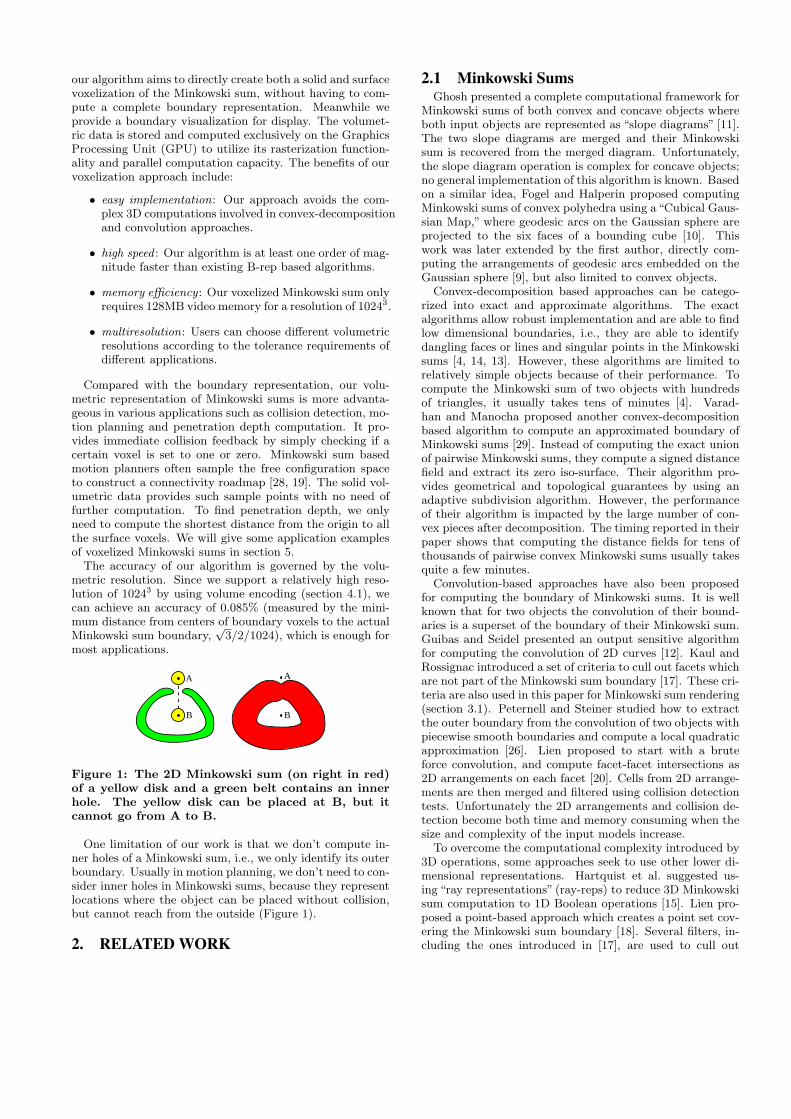
Figure 1: The 2D Minkowski sum (on right in red)of a yellow disk and a green belt contains an innerhole. The yellow disk can be placed at B, but itcannot go from A to B.

One limitation of our work is that we don’t compute in-ner holes of a Minkowski sum, i.e., we only identify its outerboundary. Usually in motion planning, we don’t need to con-sider inner holes in Minkowski sums, because they representlocations where the object can be placed without collision,but cannot reach from the outside (Figure 1).

2. RELATED WORK

2.1 Minkowski SumsGhosh presented a complete computational framework for

Minkowski sums of both convex and concave objects whereboth input objects are represented as “slope diagrams” [11].The two slope diagrams are merged and their Minkowskisum is recovered from the merged diagram. Unfortunately,the slope diagram operation is complex for concave objects;no general implementation of this algorithm is known. Basedon a similar idea, Fogel and Halperin proposed computingMinkowski sums of convex polyhedra using a“Cubical Gaus-sian Map,” where geodesic arcs on the Gaussian sphere areprojected to the six faces of a bounding cube [10]. Thiswork was later extended by the first author, directly com-puting the arrangements of geodesic arcs embedded on theGaussian sphere [9], but also limited to convex objects.

Convex-decomposition based approaches can be catego-rized into exact and approximate algorithms. The exactalgorithms allow robust implementation and are able to findlow dimensional boundaries, i.e., they are able to identifydangling faces or lines and singular points in the Minkowskisums [4, 14, 13]. However, these algorithms are limited torelatively simple objects because of their performance. Tocompute the Minkowski sum of two objects with hundredsof triangles, it usually takes tens of minutes [4]. Varad-han and Manocha proposed another convex-decompositionbased algorithm to compute an approximated boundary ofMinkowski sums [29]. Instead of computing the exact unionof pairwise Minkowski sums, they compute a signed distancefield and extract its zero iso-surface. Their algorithm pro-vides geometrical and topological guarantees by using anadaptive subdivision algorithm. However, the performanceof their algorithm is impacted by the large number of con-vex pieces after decomposition. The timing reported in theirpaper shows that computing the distance fields for tens ofthousands of pairwise convex Minkowski sums usually takesquite a few minutes.

Convolution-based approaches have also been proposedfor computing the boundary of Minkowski sums. It is wellknown that for two objects the convolution of their bound-aries is a superset of the boundary of their Minkowski sum.Guibas and Seidel presented an output sensitive algorithmfor computing the convolution of 2D curves [12]. Kaul andRossignac introduced a set of criteria to cull out facets whichare not part of the Minkowski sum boundary [17]. These cri-teria are also used in this paper for Minkowski sum rendering(section 3.1). Peternell and Steiner studied how to extractthe outer boundary from the convolution of two objects withpiecewise smooth boundaries and compute a local quadraticapproximation [26]. Lien proposed to start with a bruteforce convolution, and compute facet-facet intersections as2D arrangements on each facet [20]. Cells from 2D arrange-ments are then merged and filtered using collision detectiontests. Unfortunately the 2D arrangements and collision de-tection become both time and memory consuming when thesize and complexity of the input models increase.

To overcome the computational complexity introduced by3D operations, some approaches seek to use other lower di-mensional representations. Hartquist et al. suggested us-ing “ray representations” (ray-reps) to reduce 3D Minkowskisum computation to 1D Boolean operations [15]. Lien pro-posed a point-based approach which creates a point set cov-ering the Minkowski sum boundary [18]. Several filters, in-cluding the ones introduced in [17], are used to cull out

points that are not on the Minkowski sum boundary.Some algorithms have also been introduced for handling

specific types of objects. Seong et al. presented an algo-rithm for computing Minkowski sums of surfaces generatedby slope-monotone curves [27]. Muhlthaler and Pottmannintroduced an explicit parameterization of the convolutionof two ruled surfaces [24]. Recently Barki et al. proposedan approach for computing the Minkowski sum of a convexpolyhedron and a non-convex polyhedron whose boundary iscompletely recoverable from three orthogonal projections [1].

2.2 GPU-based VoxelizationVoxelization is the process of generating a volumetric rep-

resentation for geometric objects. In this section we brieflyreview several GPU-based voxelization algorithms that arerelated to the techniques we use in this paper. Voxeliza-tion algorithms can be classified into surface voxelizationand solid voxelization, depending on whether they voxelizeonly the boundary surface or the whole interior. Most al-gorithms described below work for both surface and solidvoxelizations. Another classification is binary voxelizationwhere each voxel is represented by 0 or 1 and non-binaryvoxelization where each voxel is represented by a real valuein [0, 1]. In this paper, we only consider binary voxelizations.

Karabassi et al. presented a depth buffer based voxeliza-tion algorithm [16]. The object is projected to the six facesof its bounding box and depth information is then read backfrom the depth buffer and used to reconstruct the object. Itworks only for an object whose boundary can be completelyseen from the six orthogonal directions. In the algorithmproposed by Fang and Chen, the object is rendered slice byslice along the z direction, and each slice is voxelized indi-vidually [7]. However, surfaces parallel (or nearly parallel)to the projection direction are not voxelized, and the mem-ory cost for high resolution volume is high since each voxelrequires one byte of memory. To solve these problems Donget al. proposed projecting the model along three orthogonaldirections and encoding multiple voxels in one texel [6].

3. RENDERING MINKOWSKI SUMSIn this section we introduce a GPU-based algorithm for

rendering the outer boundaries of Minkowski sums, withouthaving to compute a correct and complete boundary repre-sentation. The voxelization algorithm, with applications tomotion planning and penetration depth computation thatwill be discussed later in section 4 and 5, is built upon therendering results. The rendering algorithm described herecan also be used as a standalone visualization system for 3DMinkowski sums. It can also be directly applied to imple-ment the polyhedron interpolation and morphing introducedin [17].

We first introduce the terminology used in this section.We assume the two input polyhedra A and B are 2-manifoldtriangular meshes. Let FA = {fA} and FB = {fB} be theboundary triangle sets, EA = {eA} and EB = {eB} be theedge sets, and VA = {vA} and VB = {vB} be the vertex setsof A and B respectively.

The rendering algorithm first computes a set of surfaceprimitives that is a superset of the Minkowski sum boundary.Surface primitives that do not contribute to the boundaryare culled out in parallel on the GPU. The remaining prim-itives are written to a VBO (Vertex Buffer Object), whichis then rendered directly using OpenGL.

3.1 Surface Primitive CullingIt has been shown in [17] that any facet on the boundary

of A ⊕ B is generated in one of the following three ways:translating a triangle in FA by a vector in VB , translating atriangle in FB by a vector in VA, or sweeping an edge in EA

along an edge in EB . We call the triangles formed by thefirst two methods triangle primitives, and the quadrilateralsformed by the third method quadrilateral primitives.

The counts of all the triangle and quadrilateral primitivesare |FA| × |VB | + |VA| × |FB | and |EA| × |EB | respectively.These numbers are as high as millions for two polyhedrawith thousands of triangles. It will take a large amount oftime and memory to render all these primitives. For exam-ple, 1 GB memory will limit the size of A and B to just a fewthousands of triangles. Note, however, that a large numberof surface primitives lie entirely inside the Minkowski sumand will be hidden during the rendering (see Figure 2 for a2D example). We can cull out these primitives and renderonly the remaining ones. As to be shown in Table 1, this willgreatly reduce the number of primitives to be rendered. Inaddition to these completely hidden primitives, some prim-itives are trimmed by others and become partially hiddenduring the rendering (Figure 2). Convolution-based algo-rithms for computing the Minkowski sum boundary identifyand compute all such intersections, but for the purpose ofrendering, we allow them to be handled automatically in thegraphics pipeline by using the appropriate depth test.

=

Figure 2: A 2D example of surface primitives in theinterior of the Minkowski sum (shown as red lines)and trimmed surface primitives (shown as dashedlines).

In the following we call a surface primitive valid if its in-tersection with the Minkowski sum boundary has a non-zeroarea (so a partially trimmed primitive is valid since it hasa partial overlap with the Minkowski sum boundary); oth-erwise we call it invalid. Valid primitives will contribute tothe boundary of the Minkowski sum, but invalid ones willnot. Note that according to our definition, a surface primi-tive that only shares an edge or vertex with the Minkowskisum boundary is not valid, because their intersection has anarea of zero.

The rendering algorithm developed in this paper is basedon several propositions for primitive culling. The first twopropositions (Proposition 1 and 2 below) were first intro-duced in [17]. However, no proof was provided in that pa-per. These two propositions were used later, also unproved,in other works [18, 20]. In [21] the authors proved similarpropositions, but their criterion for triangle primitive cullingis weaker than the one stated below (Proposition 1). Herewe use a mathematical description and give proofs of thesetwo propositions.

Proposition 1. Given fA ∈ FA and vB ∈ VB, with nA

the outward facing normal of fA, and ei the i-th incident

=

nA

fA vB

ek

HS(P)

P

eie1

... ...

...

fA

eA

eBe0 e1

e2

e3

Prism

f 0 f1 f 2

f3

ek

Prism

Prism

fA vB

HS(P) vB

f 0 eB

f3 eA

eA eB

A

B

A

B

eA eB

eA eB

ca b

eA eB (or its reverse)

(i)

(ii)

(iii)

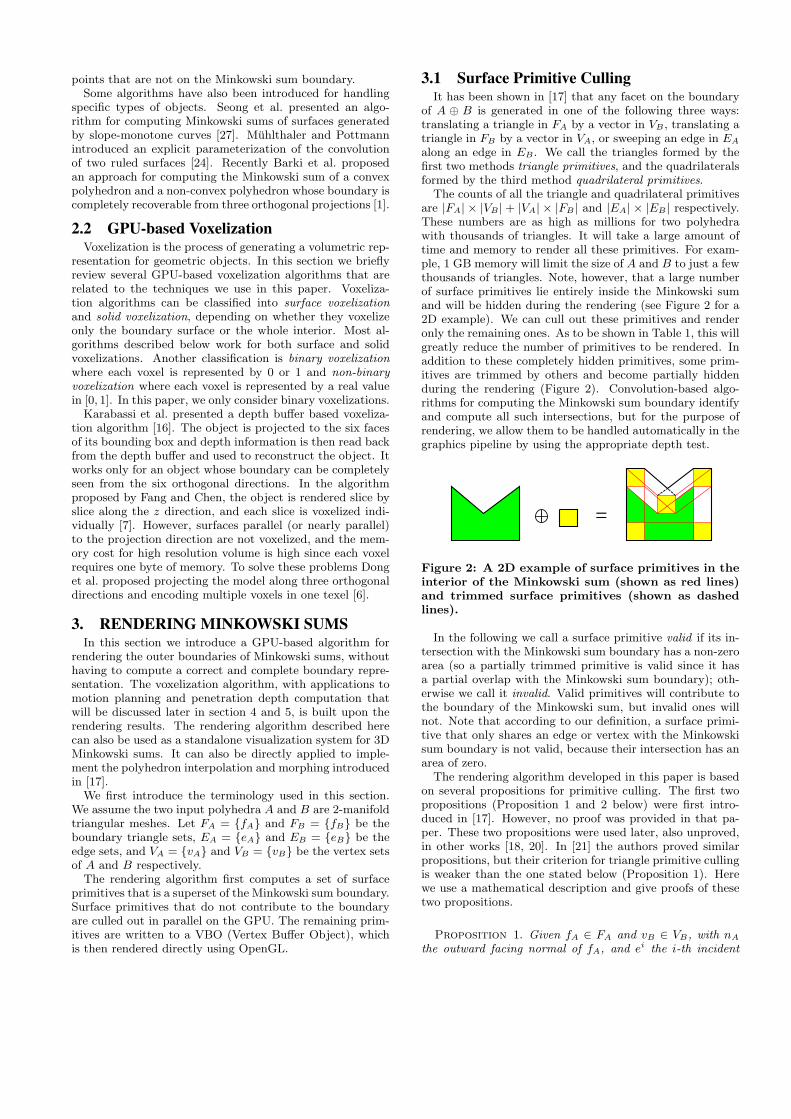
Figure 3: Illustration for proofs of Props 1, 2, and 3.

edge pointing away from vB. If fA ⊕ vB is a valid triangleprimitive, then nA · ei ≤ 0, ∀ei.

Proof. (By contradiction.) Suppose ∃ek such that nA ·ek > 0 (Figure 3 top). Since A is a 2-manifold, for any pointP inside the triangle fA, we can find a hemisphere HS(P )with a small radius r, centered at P and entirely inside A,i.e.,

HS(P ) = {Q : ‖Q− P‖ ≤ r, (Q− P ) · nA ≤ 0}HS(P ) ⊆ A.

Then we consider the translated hemisphere HS(P )⊕vB andthe prism generated by fA ⊕ ek. They locate on differentsides of the triangle fA⊕ vB (shaded in the figure). Since Pis inside fA, we can always reduce the radius of HS(P ) suchthat the other half of the hemisphere HS(P )⊕ vB is entirelyinside the prism fA ⊕ ek. This means that for each pointinside the triangle fA⊕vB , we can always find a small spherearound it and the sphere is a subset of A ⊕ B (rememberthat HS(P )⊕ vB ⊆ A⊕ vB ⊆ A⊕B and fA ⊕ ek ⊆ A⊕B).So fA ⊕ vB will not overlap with the boundary of A ⊕ B.This contradicts the assumption that fA ⊕ vB is valid.

Proposition 2. Suppose eA ∈ EA and eB ∈ EB, f0 andf1 are the two incident triangles of eA, and e0 (or e1) is oneof the two edges of f0 (or f1) pointing away from eA. Letf2, f3, e2 and e3 be defined similarly for eB. If eA⊕eB is avalid quadrilateral primitive, then either (eA × eB) · ei ≤ 0,∀ei or (eA × eB) · ei ≥ 0, ∀ei, i ∈ {0, 1, 2, 3}.

Proof. (By contradiction.) Suppose (eA × eB) · e0 > 0and (eA × eB) · e3 < 0 (the other cases can be proved sim-ilarly). We consider the two prisms generated by f0 ⊕ eB

and f3⊕eA (Figure 3 middle). They share the quadrilateraleA ⊕ eB (shaded in the figure) and locate on different sidesof it. Since both prisms are subsets of A ⊕ B, eA ⊕ eB willnot overlap with the boundary of A ⊕ B. This contradictsthe assumption that eA ⊕ eB is valid.

The above two propositions only check the relative posi-tions of incident triangles. In this paper we introduce twonew propositions that check the orientation of incident tri-angles. Since the proof of these two propositions are almostidentical, we only present the proof of the first.

Proposition 3. Suppose eA ∈ EA and eB ∈ EB. If ei-ther eA or eB is a concave edge, then eA ⊕ eB cannot be avalid quadrilateral primitive.

Proof. (By contradiction.) Suppose eA ⊕ eB is valid,then eA ⊕ eB at least partially overlaps with the boundaryof A⊕ B. Then there must exist a point c ∈ eA ⊕ eB , suchthat c is on the boundary of A⊕ B but not on any edge orvertex of the boundary (Figure 3 bottom). Then c is either alocal maximum or a local minimum of A⊕B in the directionof eA×eB . Suppose c = a+b, a ∈ eA and b ∈ eB , then botha and b should also be local maximum or minimum of A andB respectively in the direction of eA × eB . This cannot betrue if either eA or eB is a concave edge.

Proposition 4. Suppose fA ∈ FA and vB ∈ VB. If vB

is a concave vertex, then fA ⊕ vB cannot be a valid triangleprimitive.

Proof. As for Proposition 3.

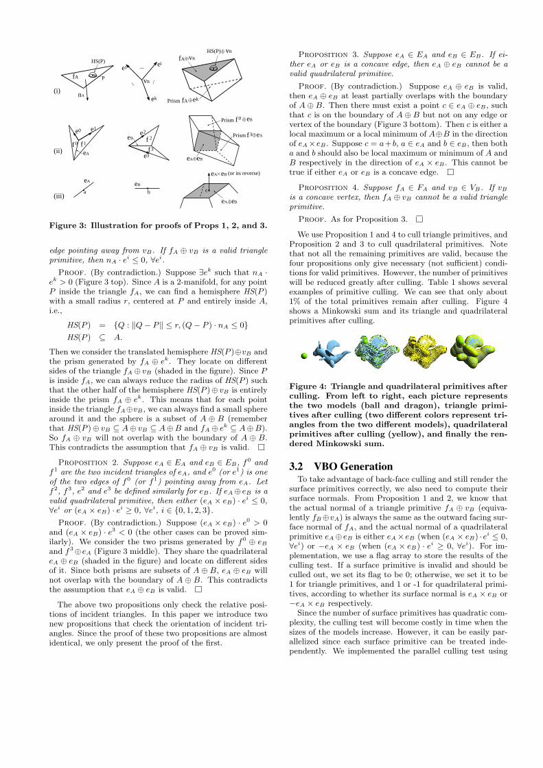
We use Proposition 1 and 4 to cull triangle primitives, andProposition 2 and 3 to cull quadrilateral primitives. Notethat not all the remaining primitives are valid, because thefour propositions only give necessary (not sufficient) condi-tions for valid primitives. However, the number of primitiveswill be reduced greatly after culling. Table 1 shows severalexamples of primitive culling. We can see that only about1% of the total primitives remain after culling. Figure 4shows a Minkowski sum and its triangle and quadrilateralprimitives after culling.

Figure 4: Triangle and quadrilateral primitives afterculling. From left to right, each picture representsthe two models (ball and dragon), triangle primi-tives after culling (two different colors represent tri-angles from the two different models), quadrilateralprimitives after culling (yellow), and finally the ren-dered Minkowski sum.

3.2 VBO GenerationTo take advantage of back-face culling and still render the

surface primitives correctly, we also need to compute theirsurface normals. From Proposition 1 and 2, we know thatthe actual normal of a triangle primitive fA ⊕ vB (equiva-lently fB⊕vA) is always the same as the outward facing sur-face normal of fA, and the actual normal of a quadrilateralprimitive eA⊕ eB is either eA× eB (when (eA × eB) · ei ≤ 0,∀ei) or −eA × eB (when (eA × eB) · ei ≥ 0, ∀ei). For im-plementation, we use a flag array to store the results of theculling test. If a surface primitive is invalid and should beculled out, we set its flag to be 0; otherwise, we set it to be1 for triangle primitives, and 1 or -1 for quadrilateral primi-tives, according to whether its surface normal is eA × eB or−eA × eB respectively.

Since the number of surface primitives has quadratic com-plexity, the culling test will become costly in time when thesizes of the models increase. However, it can be easily par-allelized since each surface primitive can be treated inde-pendently. We implemented the parallel culling test using

#tri of A #tri of B#tri primitives #quad primitives #total primitives

before culling after culling % before culling after culling % %500 2,116 1.1 M 20 K 1.82% 2.4 M 11 K 0.46% 0.89%500 12,396 6.2 M 42 K 0.68% 13.9 M 27 K 0.19% 0.34%

2,116 12,396 26.3 M 567 K 2.16% 59.0 M 350 K 0.59% 1.08%

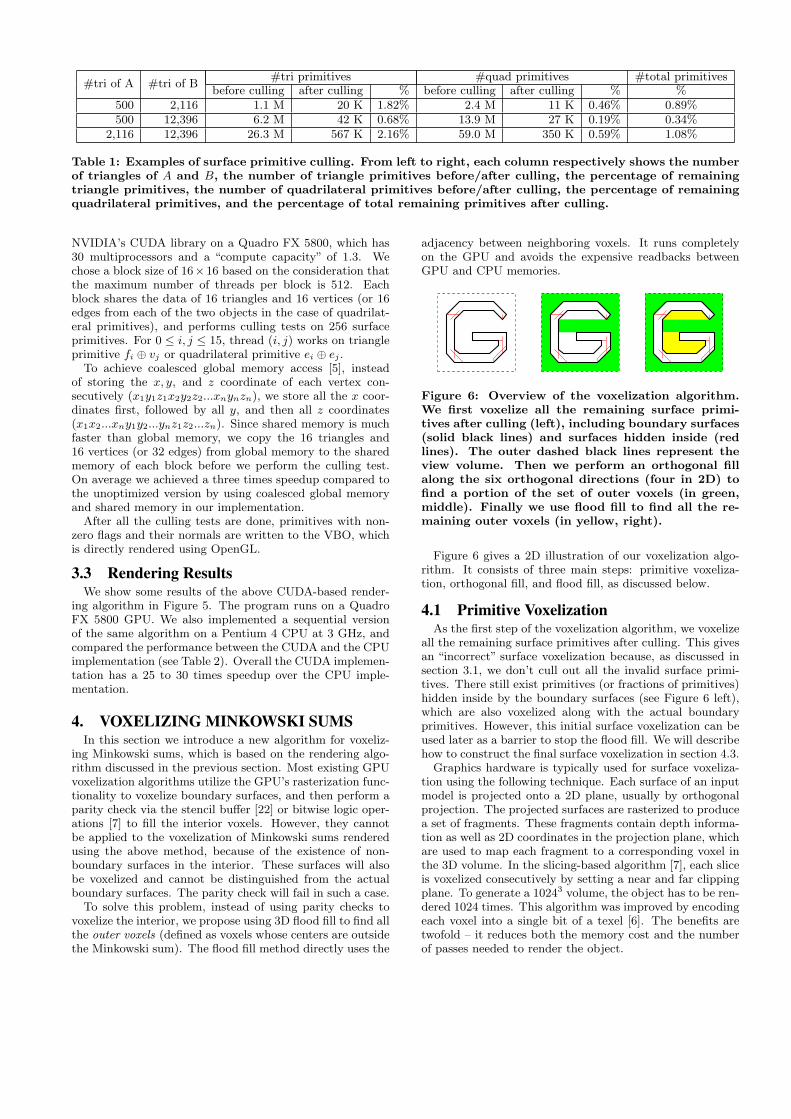
Table 1: Examples of surface primitive culling. From left to right, each column respectively shows the numberof triangles of A and B, the number of triangle primitives before/after culling, the percentage of remainingtriangle primitives, the number of quadrilateral primitives before/after culling, the percentage of remainingquadrilateral primitives, and the percentage of total remaining primitives after culling.

NVIDIA’s CUDA library on a Quadro FX 5800, which has30 multiprocessors and a “compute capacity” of 1.3. Wechose a block size of 16×16 based on the consideration thatthe maximum number of threads per block is 512. Eachblock shares the data of 16 triangles and 16 vertices (or 16edges from each of the two objects in the case of quadrilat-eral primitives), and performs culling tests on 256 surfaceprimitives. For 0 ≤ i, j ≤ 15, thread (i, j) works on triangleprimitive fi ⊕ vj or quadrilateral primitive ei ⊕ ej .

To achieve coalesced global memory access [5], insteadof storing the x, y, and z coordinate of each vertex con-secutively (x1y1z1x2y2z2...xnynzn), we store all the x coor-dinates first, followed by all y, and then all z coordinates(x1x2...xny1y2...ynz1z2...zn). Since shared memory is muchfaster than global memory, we copy the 16 triangles and16 vertices (or 32 edges) from global memory to the sharedmemory of each block before we perform the culling test.On average we achieved a three times speedup compared tothe unoptimized version by using coalesced global memoryand shared memory in our implementation.

After all the culling tests are done, primitives with non-zero flags and their normals are written to the VBO, whichis directly rendered using OpenGL.

3.3 Rendering ResultsWe show some results of the above CUDA-based render-

ing algorithm in Figure 5. The program runs on a QuadroFX 5800 GPU. We also implemented a sequential versionof the same algorithm on a Pentium 4 CPU at 3 GHz, andcompared the performance between the CUDA and the CPUimplementation (see Table 2). Overall the CUDA implemen-tation has a 25 to 30 times speedup over the CPU imple-mentation.

4. VOXELIZING MINKOWSKI SUMSIn this section we introduce a new algorithm for voxeliz-

ing Minkowski sums, which is based on the rendering algo-rithm discussed in the previous section. Most existing GPUvoxelization algorithms utilize the GPU’s rasterization func-tionality to voxelize boundary surfaces, and then perform aparity check via the stencil buffer [22] or bitwise logic oper-ations [7] to fill the interior voxels. However, they cannotbe applied to the voxelization of Minkowski sums renderedusing the above method, because of the existence of non-boundary surfaces in the interior. These surfaces will alsobe voxelized and cannot be distinguished from the actualboundary surfaces. The parity check will fail in such a case.

To solve this problem, instead of using parity checks tovoxelize the interior, we propose using 3D flood fill to find allthe outer voxels (defined as voxels whose centers are outsidethe Minkowski sum). The flood fill method directly uses the

adjacency between neighboring voxels. It runs completelyon the GPU and avoids the expensive readbacks betweenGPU and CPU memories.

axis

8.0 5.8 2.2 2.1 2.7 1.6 1.7 8.0

1.00 0.73 0.28 0.26 0.34 0.20 0.21 1.00

0

1

0.125

0.250

0.375

0.500

0.625

0.750

0.875

depth

depth buffer

axis

8.0 5.8 2.2 2.1 2.7 1.2 1.7 8.0

1.00 0.73 0.28 0.26 0.34 0.20 0.21 1.00

0

8

1

2

3

4

5

6

7

depth

depth buffer

A

A

B

B

G

G

R

R

1

2 3

1 1 1 1 1

2

1 1

2 2

4 3 3

Figure 6: Overview of the voxelization algorithm.We first voxelize all the remaining surface primi-tives after culling (left), including boundary surfaces(solid black lines) and surfaces hidden inside (redlines). The outer dashed black lines represent theview volume. Then we perform an orthogonal fillalong the six orthogonal directions (four in 2D) tofind a portion of the set of outer voxels (in green,middle). Finally we use flood fill to find all the re-maining outer voxels (in yellow, right).

Figure 6 gives a 2D illustration of our voxelization algo-rithm. It consists of three main steps: primitive voxeliza-tion, orthogonal fill, and flood fill, as discussed below.

4.1 Primitive VoxelizationAs the first step of the voxelization algorithm, we voxelize

all the remaining surface primitives after culling. This givesan “incorrect” surface voxelization because, as discussed insection 3.1, we don’t cull out all the invalid surface primi-tives. There still exist primitives (or fractions of primitives)hidden inside by the boundary surfaces (see Figure 6 left),which are also voxelized along with the actual boundaryprimitives. However, this initial surface voxelization can beused later as a barrier to stop the flood fill. We will describehow to construct the final surface voxelization in section 4.3.

Graphics hardware is typically used for surface voxeliza-tion using the following technique. Each surface of an inputmodel is projected onto a 2D plane, usually by orthogonalprojection. The projected surfaces are rasterized to producea set of fragments. These fragments contain depth informa-tion as well as 2D coordinates in the projection plane, whichare used to map each fragment to a corresponding voxel inthe 3D volume. In the slicing-based algorithm [7], each sliceis voxelized consecutively by setting a near and far clippingplane. To generate a 10243 volume, the object has to be ren-dered 1024 times. This algorithm was improved by encodingeach voxel into a single bit of a texel [6]. The benefits aretwofold – it reduces both the memory cost and the numberof passes needed to render the object.

A:A:

B:

A⊕B:

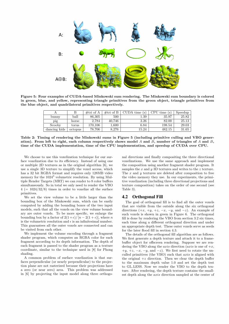
Figure 5: Four examples of CUDA-based Minkowski sum rendering. The Minkowski sum boundary is coloredin green, blue, and yellow, representing triangle primitives from the green object, triangle primitives fromthe blue object, and quadrilateral primitives respectively.

A B #tri of A #tri of B CUDA time (s) CPU time (s) Speedupbunny ball 86,305 500 1.39 35.97 25.82

pig horse 2,784 40,746 3.26 82.00 25.13Scooby torus 170,106 1,600 6.84 198.54 29.03

dancing kids octopus 78,706 8,276 15.24 482.15 31.65

Table 2: Timing of rendering the Minkowski sums in Figure 5 (including primitive culling and VBO gener-ation). From left to right, each column respectively shows model A and B, number of triangles of A and B,time of the CUDA implementation, time of the CPU implementation, and speedup of CUDA over CPU.

We choose to use this voxelization technique for our sur-face voxelization due to its efficiency. Instead of using oneor multiple 2D textures as in the original algorithm [6], weuse a single 3D texture to simplify the voxel access, whichhas a 32 bit RGBA format and requires only 128MB videomemory for the 10243 volumetric resolution. By using Mul-tiple Render Targets (MRT) we can render to 8 color bufferssimultaneously. So in total we only need to render the VBO4 (= 1024/32/8) times in order to voxelize all the surfaceprimitives.

We set the view volume to be a little larger than thebounding box of the Minkowski sum, which can be easilycomputed by adding the bounding boxes of the two inputmodels, such that all the voxels on the view volume bound-ary are outer voxels. To be more specific, we enlarge thebounding box by a factor of 2(1+ ε)/ [n− 2(1 + ε)], where nis the volumetric resolution and ε is an infinitesimal number.This guarantees all the outer voxels are connected and canbe visited from each other.

We implement the volume encoding through a fragmentshader program, which computes an RGBA color for eachfragment according to its depth information. The depth ofeach fragment is passed to the shader program as a texturecoordinate, similar to the technique used in [8] for Phongshading.

A common problem of surface voxelization is that sur-faces perpendicular (or nearly perpendicular) to the projec-tion plane are not rasterized because their projections havea zero (or near zero) area. This problem was addressedin [6] by projecting the input model along three orthogo-

nal directions and finally compositing the three directionalvoxelizations. We use the same approach and implementthe composition using another fragment shader program. Itsamples the x and y 3D textures and writes to the z texture.The x and y textures are deleted after composition to freethe video memory they use. In our experiments, the primi-tive voxelization (including three directional projections andtexture composition) takes on the order of one second (seeTable 3).

4.2 Orthogonal FillThe goal of orthogonal fill is to find all the outer voxels

that are visible from the outside along the six orthogonaldirections (+x, +y, +z, −x, −y, and −z). An example ofsuch voxels is shown in green in Figure 6. The orthogonalfill is done by rendering the VBO from section 3.2 six times,each time along a different orthogonal direction and underan appropriate depth test. These outer voxels serve as seedsfor the later flood fill in section 4.3.

The details of the orthogonal fill algorithm are as follows.We first generate a depth texture and attach it to a frame-buffer object for offscreen rendering. Suppose we are ren-dering the VBO along the axis direction (axis is one of +x,+y, +z, −x, −y, and −z). We first need to rotate the un-culled primitives (the VBO) such that axis is aligned withthe original +z direction. Then we clear the depth bufferto the maximum depth value 1.0 and set the depth testto GL LESS. Now we render the VBO to the depth tex-ture. After rendering, the depth texture contains the small-est depth along the axis direction sampled at the center of

each pixel (Figure 7). Then we identify all the voxels witha depth (at their centers) no larger than the correspondingstored value in the depth texture as outer voxels, and writean appropriate RGBA color to a 3D texture for each pixel.For example, for the pixel with a smallest depth of 2.7 inFigure 7, the RGBA color is 11 10 00 00 in binary form.Here we use 1 for outer voxels and 0 otherwise. We onlyneed three such 3D textures for the orthogonal fill – eachpair of opposite directions share the same texture. Afterall six directions are computed, we composite the three di-rectional 3D textures, using the same composition shaderprogram for primitive voxelization (section 4.1).

axis

8.0 5.8 2.2 2.1 2.7 1.6 1.7 8.0

1.00 0.73 0.28 0.26 0.34 0.20 0.21 1.00

0

1

0.125

0.250

0.375

0.500

0.625

0.750

0.875

depth

depth bufferaxis

8.0 5.8 2.2 2.1 2.7 1.2 1.7 8.0

1.00 0.73 0.28 0.26 0.34 0.20 0.21 1.00

0

8

1

2

3

4

5

6

7

depth

depth buffer

A

A

B

B

G

G

R

R

1

2 3

1 1 1 1 1

2

1 1

2 2

4 3 3

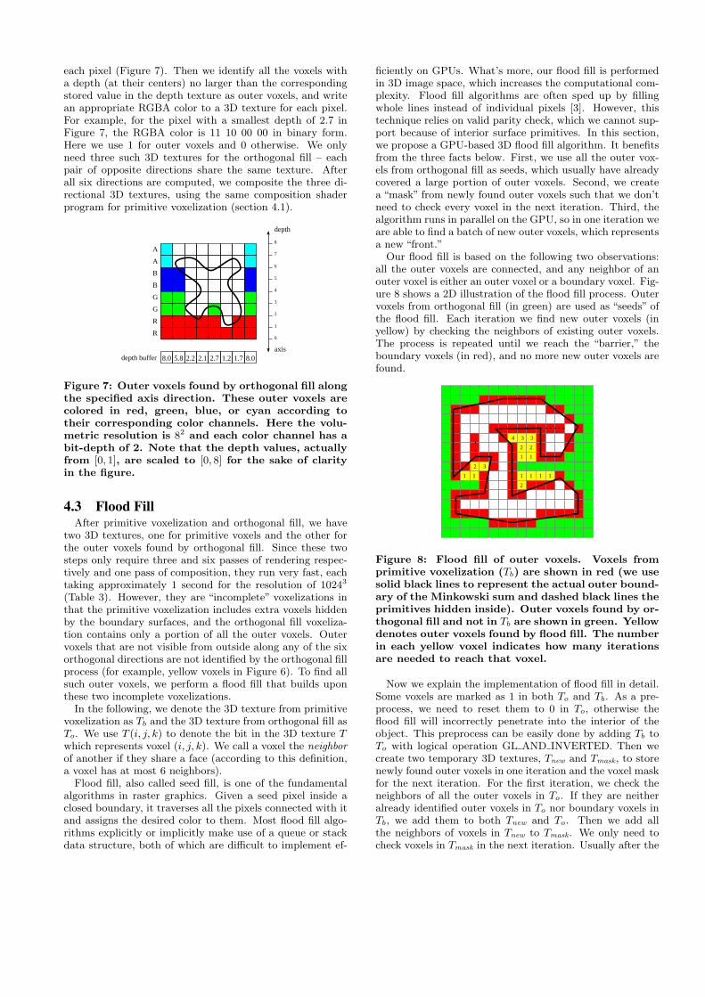
Figure 7: Outer voxels found by orthogonal fill alongthe specified axis direction. These outer voxels arecolored in red, green, blue, or cyan according totheir corresponding color channels. Here the volu-metric resolution is 82 and each color channel has abit-depth of 2. Note that the depth values, actuallyfrom [0, 1], are scaled to [0, 8] for the sake of clarityin the figure.

4.3 Flood FillAfter primitive voxelization and orthogonal fill, we have

two 3D textures, one for primitive voxels and the other forthe outer voxels found by orthogonal fill. Since these twosteps only require three and six passes of rendering respec-tively and one pass of composition, they run very fast, eachtaking approximately 1 second for the resolution of 10243

(Table 3). However, they are “incomplete” voxelizations inthat the primitive voxelization includes extra voxels hiddenby the boundary surfaces, and the orthogonal fill voxeliza-tion contains only a portion of all the outer voxels. Outervoxels that are not visible from outside along any of the sixorthogonal directions are not identified by the orthogonal fillprocess (for example, yellow voxels in Figure 6). To find allsuch outer voxels, we perform a flood fill that builds uponthese two incomplete voxelizations.

In the following, we denote the 3D texture from primitivevoxelization as Tb and the 3D texture from orthogonal fill asTo. We use T (i, j, k) to denote the bit in the 3D texture Twhich represents voxel (i, j, k). We call a voxel the neighborof another if they share a face (according to this definition,a voxel has at most 6 neighbors).

Flood fill, also called seed fill, is one of the fundamentalalgorithms in raster graphics. Given a seed pixel inside aclosed boundary, it traverses all the pixels connected with itand assigns the desired color to them. Most flood fill algo-rithms explicitly or implicitly make use of a queue or stackdata structure, both of which are difficult to implement ef-

ficiently on GPUs. What’s more, our flood fill is performedin 3D image space, which increases the computational com-plexity. Flood fill algorithms are often sped up by fillingwhole lines instead of individual pixels [3]. However, thistechnique relies on valid parity check, which we cannot sup-port because of interior surface primitives. In this section,we propose a GPU-based 3D flood fill algorithm. It benefitsfrom the three facts below. First, we use all the outer vox-els from orthogonal fill as seeds, which usually have alreadycovered a large portion of outer voxels. Second, we createa “mask” from newly found outer voxels such that we don’tneed to check every voxel in the next iteration. Third, thealgorithm runs in parallel on the GPU, so in one iteration weare able to find a batch of new outer voxels, which representsa new “front.”

Our flood fill is based on the following two observations:all the outer voxels are connected, and any neighbor of anouter voxel is either an outer voxel or a boundary voxel. Fig-ure 8 shows a 2D illustration of the flood fill process. Outervoxels from orthogonal fill (in green) are used as “seeds” ofthe flood fill. Each iteration we find new outer voxels (inyellow) by checking the neighbors of existing outer voxels.The process is repeated until we reach the “barrier,” theboundary voxels (in red), and no more new outer voxels arefound.

axis

8.0 5.8 2.2 2.1 2.7 1.6 1.7 8.0

1.00 0.73 0.28 0.26 0.34 0.20 0.21 1.00

0

1

0.125

0.250

0.375

0.500

0.625

0.750

0.875

depth

depth bufferaxis

8.0 5.8 2.2 2.1 2.7 1.2 1.7 8.0

1.00 0.73 0.28 0.26 0.34 0.20 0.21 1.00

0

8

1

2

3

4

5

6

7

depth

depth buffer

A

A

B

B

G

G

R

R

1

2 3

1 1 1 1 1

2

1 1

2 2

4 3 3

Figure 8: Flood fill of outer voxels. Voxels fromprimitive voxelization (Tb) are shown in red (we usesolid black lines to represent the actual outer bound-ary of the Minkowski sum and dashed black lines theprimitives hidden inside). Outer voxels found by or-thogonal fill and not in Tb are shown in green. Yellowdenotes outer voxels found by flood fill. The numberin each yellow voxel indicates how many iterationsare needed to reach that voxel.

Now we explain the implementation of flood fill in detail.Some voxels are marked as 1 in both To and Tb. As a pre-process, we need to reset them to 0 in To, otherwise theflood fill will incorrectly penetrate into the interior of theobject. This preprocess can be easily done by adding Tb toTo with logical operation GL AND INVERTED. Then wecreate two temporary 3D textures, Tnew and Tmask, to storenewly found outer voxels in one iteration and the voxel maskfor the next iteration. For the first iteration, we check theneighbors of all the outer voxels in To. If they are neitheralready identified outer voxels in To nor boundary voxels inTb, we add them to both Tnew and To. Then we add allthe neighbors of voxels in Tnew to Tmask. We only need tocheck voxels in Tmask in the next iteration. Usually after the

first iteration, the number of voxels we need to check will begreatly reduced. After each iteration, we employ an occlu-sion query to count the number of newly found voxels. If nonew voxels are found, the flood fill is terminated and now To

contains all the outer voxels. The pseudocode for our floodfill algorithm is given in Algorithm 1. The entire algorithmis implemented using three fragment shaders, for excludingvoxels in Tb from To, checking neighbor voxels, and creatingthe mask respectively.

Algorithm 1 FloodFill

input: To, Tb

output: To

To ← To − (To ∩ Tb)create two 3D textures Tnew and Tmask;clear all voxels of Tmask to 0;for all voxel(i,j,k) do

if at least one neighbor has value 1 in To thenTmask(i, j, k) = 1

end ifend forrepeat

clear all voxels of Tnew to 0for all voxel(i,j,k) satisfying Tmask(i, j, k) = 1 do

if To(i, j, k) = 0 and Tb(i, j, k) = 0 thenTo(i, j, k) = 1Tnew(i, j, k) = 1

end ifend forclear all voxels of Tmask to 0for all voxel(i,j,k) do

if at least one neighbor has value 1 in Tnew thenTmask(i, j, k) = 1

end ifend for

until ∀(i, j, k), Tnew(i, j, k) = 0 //test with occlusionquerydelete Tnew and Tmask

return To

After all the outer voxels are identified, it becomes veryeasy to compute a correct surface voxelization. We onlyneed to find those primitive voxels in Tb adjacent to an outervoxel. For example, in Figure 8, the final outer boundarysurface (solid black lines) consists of primitive voxels (red)which have at least one outer voxel (green or yellow) as aneighbor.

The performance of flood fill is determined by the volu-metric resolution and object complexity. For a resolutionof 512 × 512 × 512, it usually takes less than one secondfor most of the models we have tested (see Table 3). Fora resolution of 10243, the time ranges from a few to tensof seconds, depending on how many iterations we need toperform the flood fill.

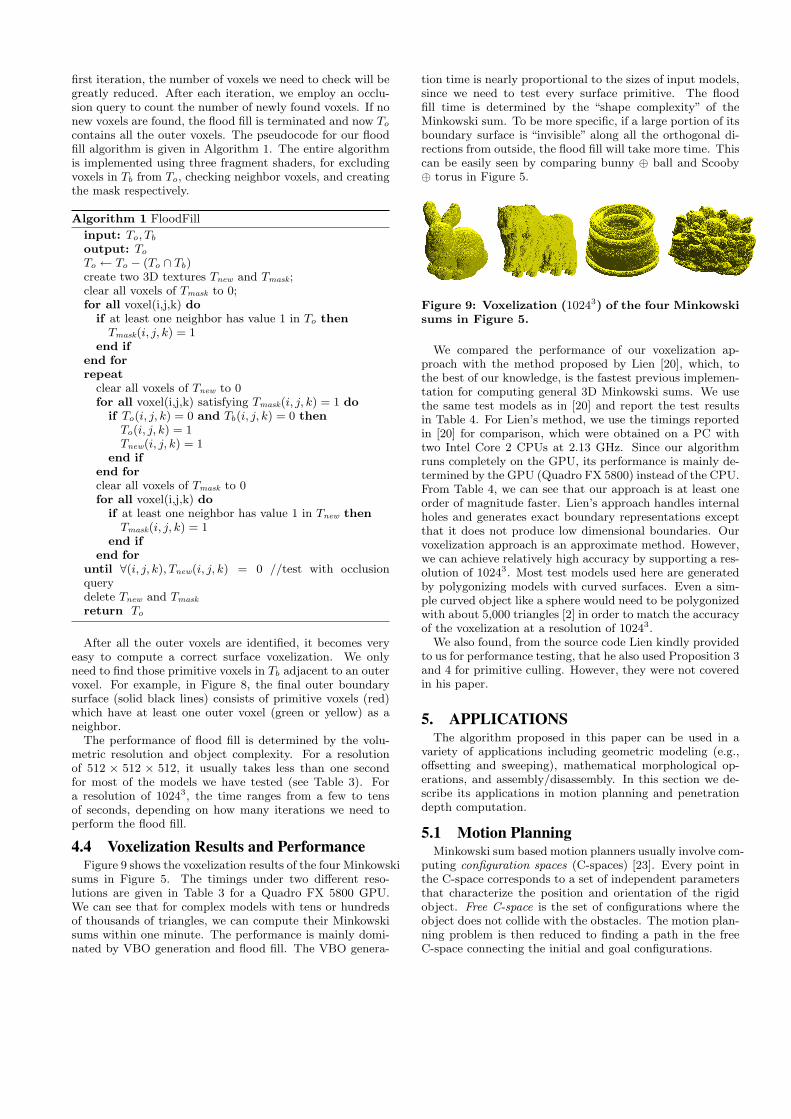
4.4 Voxelization Results and PerformanceFigure 9 shows the voxelization results of the four Minkowski

sums in Figure 5. The timings under two different reso-lutions are given in Table 3 for a Quadro FX 5800 GPU.We can see that for complex models with tens or hundredsof thousands of triangles, we can compute their Minkowskisums within one minute. The performance is mainly domi-nated by VBO generation and flood fill. The VBO genera-

tion time is nearly proportional to the sizes of input models,since we need to test every surface primitive. The floodfill time is determined by the “shape complexity” of theMinkowski sum. To be more specific, if a large portion of itsboundary surface is “invisible” along all the orthogonal di-rections from outside, the flood fill will take more time. Thiscan be easily seen by comparing bunny ⊕ ball and Scooby⊕ torus in Figure 5.

Figure 9: Voxelization (10243) of the four Minkowskisums in Figure 5.

We compared the performance of our voxelization ap-proach with the method proposed by Lien [20], which, tothe best of our knowledge, is the fastest previous implemen-tation for computing general 3D Minkowski sums. We usethe same test models as in [20] and report the test resultsin Table 4. For Lien’s method, we use the timings reportedin [20] for comparison, which were obtained on a PC withtwo Intel Core 2 CPUs at 2.13 GHz. Since our algorithmruns completely on the GPU, its performance is mainly de-termined by the GPU (Quadro FX 5800) instead of the CPU.From Table 4, we can see that our approach is at least oneorder of magnitude faster. Lien’s approach handles internalholes and generates exact boundary representations exceptthat it does not produce low dimensional boundaries. Ourvoxelization approach is an approximate method. However,we can achieve relatively high accuracy by supporting a res-olution of 10243. Most test models used here are generatedby polygonizing models with curved surfaces. Even a sim-ple curved object like a sphere would need to be polygonizedwith about 5,000 triangles [2] in order to match the accuracyof the voxelization at a resolution of 10243.

We also found, from the source code Lien kindly providedto us for performance testing, that he also used Proposition 3and 4 for primitive culling. However, they were not coveredin his paper.

5. APPLICATIONSThe algorithm proposed in this paper can be used in a

variety of applications including geometric modeling (e.g.,offsetting and sweeping), mathematical morphological op-erations, and assembly/disassembly. In this section we de-scribe its applications in motion planning and penetrationdepth computation.

5.1 Motion PlanningMinkowski sum based motion planners usually involve com-

puting configuration spaces (C-spaces) [23]. Every point inthe C-space corresponds to a set of independent parametersthat characterize the position and orientation of the rigidobject. Free C-space is the set of configurations where theobject does not collide with the obstacles. The motion plan-ning problem is then reduced to finding a path in the freeC-space connecting the initial and goal configurations.

A ⊕ B VBOPrim. Vox. Ortho. Fill Flood Fill #Flood Fill Total512 1024 512 1024 512 1024 512 1024 512 1024

bunny (86,305) ⊕ ball (500) 1.39 0.43 1.37 0.28 0.70 0.41 2.74 1 4 2.51 6.19pig (2,784) ⊕ horse (40,746) 3.26 0.15 0.66 0.13 0.55 0.49 5.76 23 111 4.02 10.23

Scooby (170,106) ⊕ torus (1,600) 6.84 0.18 0.68 0.12 0.54 0.78 8.15 44 153 7.92 16.21dancing kids (78,706) ⊕ octopus (8,276) 15.24 0.30 1.12 0.21 0.63 0.69 8.74 41 185 16.44 25.74

Table 3: Timing for voxelizing the four Minkowski sums in Figure 5 under two different resolutions (inseconds). From left to right, each column respectively shows the input models with their numbers of triangles,time for VBO generation (including primitive culling), time for primitive voxelization, time for orthogonalfill, time for flood fill, number of flood fill iterations, and total time. The “512” and “1024” subcolumnsrepresent 5123 and 10243 resolutions.

A B #tri of A #tri of B Lien’s#Flood Fill Ours Speedup512 1024 512 1024 512 1024

inner ear frame 32,236 96 202.00 161 333 2.25 16.63 90× 12×bull frame 12,396 96 289.30 120 240 1.96 13.82 148× 21×

grate1 grate2 540 942 318.50 0 0 1.88 7.66 169× 42×clutch knot 2,116 992 347.00 0 0 0.99 4.84 351× 72×bull knot 12,396 992 755.10 113 195 2.25 11.52 336× 66×

inner ear knot 32,236 992 920.80 18 140 2.03 9.70 454× 95×

Table 4: Performance comparison with Lien’s approach (in seconds). From left to right, each column re-spectively shows model A and B, number of triangles of A and B, time of Lien’s approach, number of floodfill iterations, time of our approach, and the speedup. The “512” and “1024” subcolumns represent 5123 and10243 resolutions.

The free C-space is usually computed using Minkowskisums. For P a translating object and Q the union of all theobstacles, the free C-space is the complement of Q ⊕ −P ,where −P is P reflected about the origin. In Figure 10,the free C-space of a plug and an outlet is computed usingour voxelization algorithm. This is a challenging problemsince the three legs of the plug should go into the three cor-responding holes of the outlet. Our algorithm successfullyfound the narrow passageway in the free C-space.

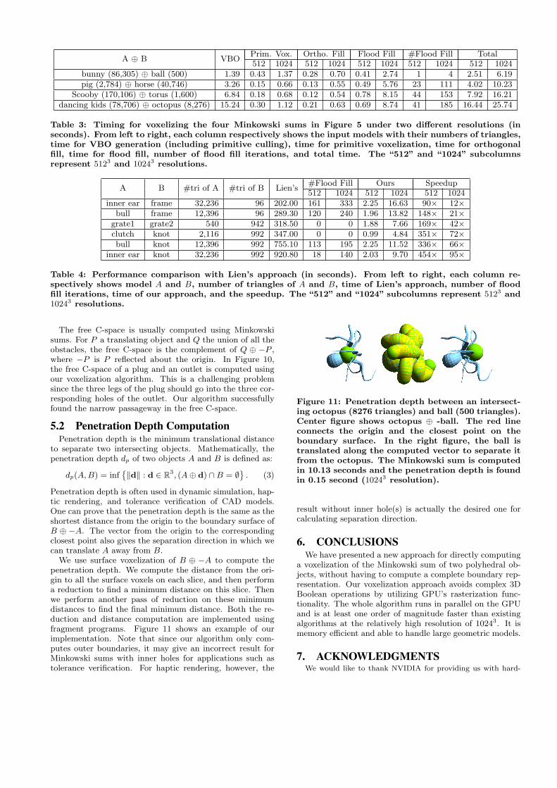
5.2 Penetration Depth ComputationPenetration depth is the minimum translational distance

to separate two intersecting objects. Mathematically, thepenetration depth dp of two objects A and B is defined as:

dp(A, B) = inf{‖d‖ : d ∈ R3, (A⊕ d) ∩B = ∅

}. (3)

Penetration depth is often used in dynamic simulation, hap-tic rendering, and tolerance verification of CAD models.One can prove that the penetration depth is the same as theshortest distance from the origin to the boundary surface ofB ⊕ −A. The vector from the origin to the correspondingclosest point also gives the separation direction in which wecan translate A away from B.

We use surface voxelization of B ⊕ −A to compute thepenetration depth. We compute the distance from the ori-gin to all the surface voxels on each slice, and then performa reduction to find a minimum distance on this slice. Thenwe perform another pass of reduction on these minimumdistances to find the final minimum distance. Both the re-duction and distance computation are implemented usingfragment programs. Figure 11 shows an example of ourimplementation. Note that since our algorithm only com-putes outer boundaries, it may give an incorrect result forMinkowski sums with inner holes for applications such astolerance verification. For haptic rendering, however, the

Figure 11: Penetration depth between an intersect-ing octopus (8276 triangles) and ball (500 triangles).Center figure shows octopus ⊕ -ball. The red lineconnects the origin and the closest point on theboundary surface. In the right figure, the ball istranslated along the computed vector to separate itfrom the octopus. The Minkowski sum is computedin 10.13 seconds and the penetration depth is foundin 0.15 second (10243 resolution).

result without inner hole(s) is actually the desired one forcalculating separation direction.

6. CONCLUSIONSWe have presented a new approach for directly computing

a voxelization of the Minkowski sum of two polyhedral ob-jects, without having to compute a complete boundary rep-resentation. Our voxelization approach avoids complex 3DBoolean operations by utilizing GPU’s rasterization func-tionality. The whole algorithm runs in parallel on the GPUand is at least one order of magnitude faster than existingalgorithms at the relatively high resolution of 10243. It ismemory efficient and able to handle large geometric models.

7. ACKNOWLEDGMENTSWe would like to thank NVIDIA for providing us with hard-

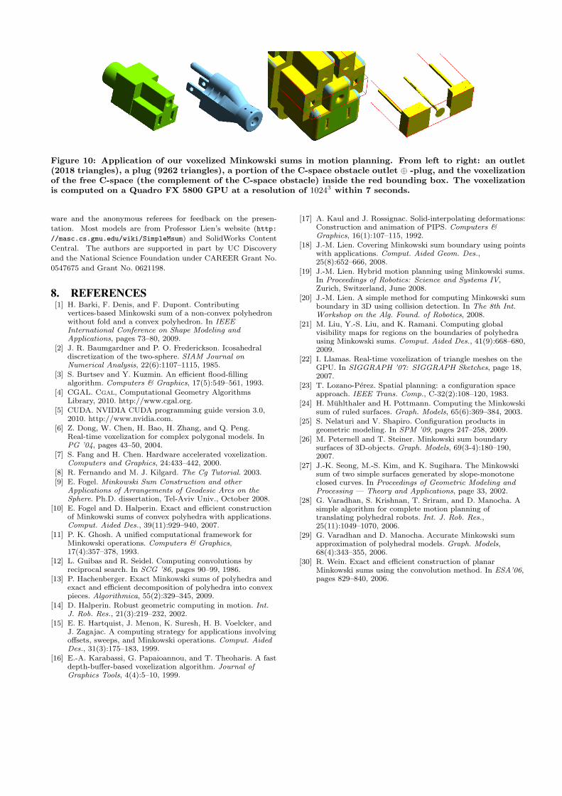
Figure 10: Application of our voxelized Minkowski sums in motion planning. From left to right: an outlet(2018 triangles), a plug (9262 triangles), a portion of the C-space obstacle outlet ⊕ -plug, and the voxelizationof the free C-space (the complement of the C-space obstacle) inside the red bounding box. The voxelizationis computed on a Quadro FX 5800 GPU at a resolution of 10243 within 7 seconds.

ware and the anonymous referees for feedback on the presen-

tation. Most models are from Professor Lien’s website (http:

//masc.cs.gmu.edu/wiki/SimpleMsum) and SolidWorks Content

Central. The authors are supported in part by UC Discovery

and the National Science Foundation under CAREER Grant No.

0547675 and Grant No. 0621198.

8. REFERENCES[1] H. Barki, F. Denis, and F. Dupont. Contributing

vertices-based Minkowski sum of a non-convex polyhedronwithout fold and a convex polyhedron. In IEEEInternational Conference on Shape Modeling andApplications, pages 73–80, 2009.

[2] J. R. Baumgardner and P. O. Frederickson. Icosahedraldiscretization of the two-sphere. SIAM Journal onNumerical Analysis, 22(6):1107–1115, 1985.

[3] S. Burtsev and Y. Kuzmin. An efficient flood-fillingalgorithm. Computers & Graphics, 17(5):549–561, 1993.

[4] CGAL. Cgal, Computational Geometry AlgorithmsLibrary, 2010. http://www.cgal.org.

[5] CUDA. NVIDIA CUDA programming guide version 3.0,2010. http://www.nvidia.com.

[6] Z. Dong, W. Chen, H. Bao, H. Zhang, and Q. Peng.Real-time voxelization for complex polygonal models. InPG ’04, pages 43–50, 2004.

[7] S. Fang and H. Chen. Hardware accelerated voxelization.Computers and Graphics, 24:433–442, 2000.

[8] R. Fernando and M. J. Kilgard. The Cg Tutorial. 2003.[9] E. Fogel. Minkowski Sum Construction and other

Applications of Arrangements of Geodesic Arcs on theSphere. Ph.D. dissertation, Tel-Aviv Univ., October 2008.

[10] E. Fogel and D. Halperin. Exact and efficient constructionof Minkowski sums of convex polyhedra with applications.Comput. Aided Des., 39(11):929–940, 2007.

[11] P. K. Ghosh. A unified computational framework forMinkowski operations. Computers & Graphics,17(4):357–378, 1993.

[12] L. Guibas and R. Seidel. Computing convolutions byreciprocal search. In SCG ’86, pages 90–99, 1986.

[13] P. Hachenberger. Exact Minkowski sums of polyhedra andexact and efficient decomposition of polyhedra into convexpieces. Algorithmica, 55(2):329–345, 2009.

[14] D. Halperin. Robust geometric computing in motion. Int.J. Rob. Res., 21(3):219–232, 2002.

[15] E. E. Hartquist, J. Menon, K. Suresh, H. B. Voelcker, andJ. Zagajac. A computing strategy for applications involvingoffsets, sweeps, and Minkowski operations. Comput. AidedDes., 31(3):175–183, 1999.

[16] E.-A. Karabassi, G. Papaioannou, and T. Theoharis. A fastdepth-buffer-based voxelization algorithm. Journal ofGraphics Tools, 4(4):5–10, 1999.

[17] A. Kaul and J. Rossignac. Solid-interpolating deformations:Construction and animation of PIPS. Computers &Graphics, 16(1):107–115, 1992.

[18] J.-M. Lien. Covering Minkowski sum boundary using pointswith applications. Comput. Aided Geom. Des.,25(8):652–666, 2008.

[19] J.-M. Lien. Hybrid motion planning using Minkowski sums.In Proceedings of Robotics: Science and Systems IV,Zurich, Switzerland, June 2008.

[20] J.-M. Lien. A simple method for computing Minkowski sumboundary in 3D using collision detection. In The 8th Int.Workshop on the Alg. Found. of Robotics, 2008.

[21] M. Liu, Y.-S. Liu, and K. Ramani. Computing globalvisibility maps for regions on the boundaries of polyhedrausing Minkowski sums. Comput. Aided Des., 41(9):668–680,2009.

[22] I. Llamas. Real-time voxelization of triangle meshes on theGPU. In SIGGRAPH ’07: SIGGRAPH Sketches, page 18,2007.

[23] T. Lozano-Perez. Spatial planning: a configuration spaceapproach. IEEE Trans. Comp., C-32(2):108–120, 1983.

[24] H. Muhlthaler and H. Pottmann. Computing the Minkowskisum of ruled surfaces. Graph. Models, 65(6):369–384, 2003.

[25] S. Nelaturi and V. Shapiro. Configuration products ingeometric modeling. In SPM ’09, pages 247–258, 2009.

[26] M. Peternell and T. Steiner. Minkowski sum boundarysurfaces of 3D-objects. Graph. Models, 69(3-4):180–190,2007.

[27] J.-K. Seong, M.-S. Kim, and K. Sugihara. The Minkowskisum of two simple surfaces generated by slope-monotoneclosed curves. In Proceedings of Geometric Modeling andProcessing — Theory and Applications, page 33, 2002.

[28] G. Varadhan, S. Krishnan, T. Sriram, and D. Manocha. Asimple algorithm for complete motion planning oftranslating polyhedral robots. Int. J. Rob. Res.,25(11):1049–1070, 2006.

[29] G. Varadhan and D. Manocha. Accurate Minkowski sumapproximation of polyhedral models. Graph. Models,68(4):343–355, 2006.

[30] R. Wein. Exact and efficient construction of planarMinkowski sums using the convolution method. In ESA’06,pages 829–840, 2006.