A goal programming capital budgeting model under...

Scientia Iranica E (2018) 25(2), 841{851

Sharif University of TechnologyScientia Iranica

Transactions E: Industrial Engineeringhttp://scientiairanica.sharif.edu

A goal programming capital budgeting model underuncertainty in construction industry

S. Etemadi, H. Koosha�, and M. Salari

Department of Industrial Engineering, Faculty of Engineering, Ferdowsi University of Mashhad, Mashhad, P.O. Box 91775-1111,Iran.

Received 13 February 2016; received in revised form 4 December 2016; accepted 19 December 2016

KEYWORDSCapital budgeting;Time horizon model;Goal programming;Fuzzy AnalyticHierarchy Process(FAHP);Construction industry.

Abstract. Due to the increase of investments in construction projects and the lack ofpractical models in this area, developing new practical models is essential. In this paper,researchers suggest a new model in which (1) Its assumptions are adopted based on the realworld, (2) Goal programming is used because of the soft nature of the budget constraints,and (3) Risk of variations in cash ows is considered. The presented model chooses themost pro�table portfolio of projects and determines their respective �nancing resources,area under construction, and pre-sale and sale amounts for each period, such that thecumulative cash ow at the end of the time horizon is maximized. The Fuzzy AnalyticHierarchy Process (FAHP) is used to determine the weight of the objectives. The exactsolution to the model is obtained using the ILOG CPLEX software. The presented solutionseems e�cient since it yields very small elapsed times to solve exactly the real-world-sizedproblems. Also, the sensitivity analysis is performed and the results are deliberately studiedand analyzed. Parameters, such as pre-sale prices, mean, and variance of the sale price andconstruction costs, are among the highly sensitive parameters.© 2018 Sharif University of Technology. All rights reserved.

1. Introduction

The construction industry is one of the most impor-tant industries in any country, since it absorbs vastinvestments and is one of the substantial needs ofthe community. Nevertheless, this industry su�ersfrom huge amounts of capital wastes caused by poorand ine�cient capital budgeting [1]. Compared toother industries, the absence of �nancial control andweak management has led to a set of undesirable andirreversible results. In addition, the bankruptcy levelis signi�cantly high which can be alleviated with a

*. Corresponding author.E-mail addresses: se [email protected] (S. Etemadi);[email protected] (H. Koosha); [email protected](M. Salari)

doi: 10.24200/sci.2017.4436

better cash ow management procedure [2]. Cash owanalysis of construction projects is an important issuein construction industry [3]. Therefore, this paperis dedicated to the capital budgeting of constructioncompanies due to the lack of applicable models in thisarea.

This research develops a model, which helpsdecision-makers in construction industry to select themost pro�table investment opportunity from a poolof available opportunities and determine the proper�nancial resources at the right time. The data froma real construction company is used in order for themodel to be more adaptive to the real world and to beable to quench the industry's expectations.

Capital budgeting is a process that allocateslimited �nancial resources to the available projectsand aims at maximizing the return on investment [4].Capital budgeting is a major problem that managesthe �nancial resources. This is usually a long-term

842 S. Etemadi et al./Scientia Iranica, Transactions E: Industrial Engineering 25 (2018) 841{851

problem involving risk complications and needs sig-ni�cant amounts of investment. The majority ofcapital budgeting decisions are irreversible. Therefore,applying proper capital budgeting models, leading intothe right decisions on choosing the right projects at theright time, is crucial to the survival of the companiesin their uncertain environment [5].

The �rst research on capital budgeting was re-ported by Lorie and Savage [6] with the goal ofmaximizing the Net Present Value (NPV). Weingart-ner [7] presented a mathematical programming modelfor the capital budgeting problem that maximizescumulative cash at the end of the time horizon, knownas horizon models. Unlike the NPV maximizationapproach, the model developed by Weingartner consid-ers di�erent �nancial resources with di�erent interestrates and transfers each period's unused budgets toits next period. In addition, the consideration ofpossible loaning, borrowing, and di�erent �nancingapproaches is amongst the noteworthy characteristicsof this model. Thus, it is very well adapting to thereal-world situations; therefore, modeling the capitalbudgeting problem through the maximization of thecumulative cash at the end of a pre-speci�ed timehorizon is preferred to the maximization of the NPV [8].

However, Weingartner's time horizon model facessome critical issues. In particular, the presence of thehard budget constraints in the model is one of theseissues. Considering each period's budget constraintas an internal functional constraint imposed by themanagement is more realistic than considering it asan external constraint imposed by the market [9].Thus, one can consider the budget constraints assoft constraints and minimize the deviation from theideal. To this end, goal programming is the mostcommon and reputable method already suggested forsuch situations.

As in the literature, all the following researchershave presented their models: Taylor and Keown [10] forpolice department budgeting, Lawrence and Reeves [11]for an insurance company, Mukherjee and Bera [12] forIndia coal industry, and Thizy et al. [13] for a Canadiantelecommunication company. In addition, Badri etal. [14] presented a binary goal-programming model forproject selection in a healthcare institute. Vashishthet al. [15] proposed a binary goal programming modelfor the capital budgeting of a hospital. None of theaforementioned studies considers the loaning, borrow-ing, and di�erent �nancing approaches with di�erentinterest rate options.

Goal programming model along with the FuzzyAnalytic Hierarchy Process (FAHP) is a supple toolto accomplish the goals under various constraints [16].Hence, neither of them is adequate for considering thenumerical and non-numerical information alone [17].The FAHP prepares a relatively mature explanation of

the decision process, including personal and imprecisejudgments of the decision-makers [18]. Chang [19]presented the Extent Analysis Method for the FAHPin which triangular fuzzy numbers for pairwise com-parisons are used. Other methods as Modi�ed DigitalLogic (MDL) and Fuzzy Decision-Making Trial andEvaluation Laboratory (FDEMATEL) are used to pri-oritize the importance of various criteria. Chaghooshiet al. [20] proposed the decision-making process ofselecting the most suitable managers for projects usingFDEMATEL method. Rathi et al. [21] developeda project selection approach to determining properSix Sigma projects in automotive companies usingthe MDL method. Ghazimoradi et al. [22] proposeda model based on neural networks to anticipate thesuccess of construction projects depending on thelevel of realization of success factors during the initialphase of a project. Tang and Chang [23] applied thegoal programming and FAHP to a capital budgetingproblem in a small car renting company. However,their model does not utilize the Weingartner's horizonmodel along with the cash ow of the investmentopportunities as the criteria for optimal investmentopportunity selection.

Another critical issue with the Weingartner'smodel is that it ignores risk and uncertainty. Thoughrisk management and capital budgeting often needto be considered jointly [24], none of the aforemen-tioned studies considers the uncertainty and risk of theprojects seldom inevitable, especially in investment-type projects.

The main goal of the portfolio optimization isto help the investor optimally allocate �nancial re-sources to the investment opportunities, such thatthe risk and uncertainty parameters are accountedfor [25]. Risk and uncertainty can be considered asa Markowitz mean-variance model [26], Capital AssetPricing Model (CAPM) [27,28,29], and Value at Risk(VaR) model [30]. Su and Huang [31] proposed a mean-variance capital budgeting model in which project pa-rameters are regarded as random variables. Babaei etal. [32] formulated the portfolio optimization problemas a multi-objective mixed integer programming inwhich VaR is speci�ed as the risk measure. Beraldi etal. [33] considered Conditional Value at Risk (CVaR) intheir capital budgeting model. Khalili-Damghani andTaghavifard [34] proposed a multi-dimensional knap-sack model for capital budgeting under uncertainty inwhich fuzzy set theory is applied.

Contrary to the Weingartner's time horizonmodel, in this article, budget constraints are consideredsoft and the capital budgeting problem for constructioncompanies is modeled in the form of goal programming.FAHP is also used to determine the weight of theobjectives.

In addition, we consider the risk in our model.

S. Etemadi et al./Scientia Iranica, Transactions E: Industrial Engineering 25 (2018) 841{851 843

Since the CAPM and VaR models need a number ofdi�cult-to-estimate parameters in the case of construc-tion companies, they do not seem suitable in this area.Hillier [35] evaluated risky investments by estimatingthe expected values and standard deviations of netcash ows for each alternative investment. Walls [36]de�ned risk as the standard deviation of returns (i.e.,net present value) of the portfolio of assets. He pointedout that this measure is more precisely de�ned as astatistical measure of uncertainty. In this study, therisk is considered rather similar to the mean-variancemodel. The only di�erence here is that instead of thecapital return, the cumulative cash ow at the end ofthe time horizon is used.

In this paper, we propose a capital budgetingmodel with considering the risk of projects in orderto apply in the construction industry. In the model,we consider time value of money and the risk of theprojects. Since the budget constraints are usuallysoft and multiple objectives are available in the realworld, goal programming is applied to cope with thissituation. Because the weights of goals in the model aredetermined by experts' estimations, the fuzzy analytichierarchy process is used for an e�cient estimation ofthe weights.

The rest of this paper is organized as follows.In the next section, the problem de�nition, modelingapproach, and the suggested mathematical model areincluded. Section 3 is dedicated to designing andexactly solving a number of sample problems. Thesensitivity analysis results of the model and interpreta-tion of the results are presented in Section 4. Finally,conclusions and future research directions are providedin Section 5.

2. Problem de�nition and modeling

In this section, we develop a formal description ofthe problem. In particular, two models, includinga single-objective mixed integer programming and amixed integer goal programming model, are presented.

2.1. Problem de�nitionThe problem is based on the data from a constructioncompany. According to the geographical position ofthe projects and the municipality requirements, themaximum allowed construction area for each projectis known. The scope of the projects is limited toconstruction of the residential and commercial units.The construction time of the projects varies between24 to 30 months or 8 to 10 time periods, where eachperiod consists of 3 months.

The construction costs can be categorized intotwo groups, including �xed and variable costs. The�xed cost is independent of the construction area, whilevariable costs depend on the construction area. The

variable costs in the construction industry are usuallyhigher than the �xed costs.

Financing of a project is possible through a setof resources including the capital from the investors,loans, and the pre-sale of some parts of the project.Two types of interest rates are considered. In par-ticular, one is the interest rate of the bank, and theother is the lending interest rate for the cases towhich the company lends money (external investmentopportunities) and the return of the cash ows fromthe sale unit. At each time period, there is a limit onthe maximum amount of money loaned from the bank.This bound is a pre-speci�ed percent of the money fromthe investors up to that period.

2.2. Model developmentTo �nd the ideal values for risk and cash at the endof the time horizon, we suggest solving the single-objective model. By solving the single-objective model,the range of the ideal values for the maximization ofthe cumulative cash at the end of the time horizonand an upper bound for the risk constraint are deter-mined; both are considered as parameters of the goal-programming model.

The model assumptions are as follows:

1. The unit material and equipment cost (price) areconstants during the periods of construction;

2. The remaining area from the whole pre-sale of aproject is sold equally in sale periods;

3. The lending (external investment) interest rate andthe interest rate of the returning cash ows fromsale are assumed the same;

4. The end of the time horizon, at which the sum ofthe cumulative cash is maximized, is considered asthe �nal construction period.

Parameters of the modelJ Set of projectsI Set of tools (equipment)L Set of construction time periodsN End of the time horizonH Set of sale time periodsk Number of sale periodsn0 The period at which the sum of all the

cash ows up to that period must bepositive without considering the timevalue of money, n0 < N

fj In ation rate for the selling price ofone square meter of project j

rl The interest rate of lending andreturning the cash ows from sale(beyond the time horizon)

rb Bank loan interest rate


�pjs Mean sale price of one area unit ofproject j in the �rst time period afterthe accomplishment of project j

�pjs Sale price variance ( uctuations) of oneunit area of project j in the �rst timeperiod after the accomplishment ofproject j (risk measure of the projectj)

pjn Pre-sale price of project j in period n(for each area unit)

Fjn Fixed construction cost of project j inperiod n

mjin Required amount of material andequipment of type i for project j inperiod n

cji Unit cost of material and equipment oftype i for project j

Kj Maximum allowed construction areafor project j

Mn Maximum available budget of investorsin period n

B1n Maximum allowed bank-loan-type�nancing in period n

�jn Allowed pre-sale percentage of projectj in period n

P Risk constraint upper boundwg Penalty for the deviation of the

cumulative cash in period Nwn Penalty for the deviation of the budget

constraint in period nwn0 Penalty for the deviation of the \sum

of cash ow positivity up to n0"constraint from the speci�ed ideal

G The ideal cumulative cash in period N

vjn =Pri=1mjincji Variable construction cost of

project j in period n

Decision variablesxj Binary variable equals to 1 if project j

is selected and 0 otherwiseyj Total construction area for project j

vn Lending value (external investment)from period n to n+ 1

w1n Loaned value of the bank from periodn to n+ 1

w2jn Pre-sale value of project j in period n

d�g ; (d+g ) Decision variable for negative (positive)

cumulative cash deviation in period Nfrom the speci�ed ideal

d�n ; (d+n ) Decision variable for negative (positive)

budget constraint deviation in periodn from the speci�ed ideal

d�n0 ; (d+n0) Decision variable for negative (positive)

deviation of the \sum of cash owpositivity up to n0" constraint from thespeci�ed ideal

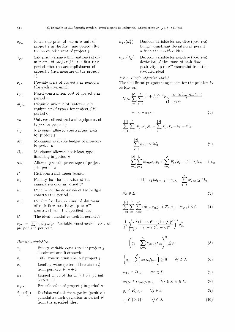
2.2.1. Single objective modelThe non-linear programming model for the problem isas follows:

MaxjJjXj=1

kXh=1

(1 + fj)h�1�pjs(yj�PN

n=0 w2jn=pjn)k

(1 + rl)h

+ �N � w1N ; (1)

jJjXj=1

jIjXi=1

mji0cjiyj +jJjXj=1

Fj0xj + �0 � w10

�jJjXj=1

w2j0 �M0; (2)

jJjXj=1

jIjXi=1

mjincjiyj +jJjXj=1

Fjnxj � (1 + rl)�n�1 + �n

+ (1 + rb)w1;n�1 � w1n �jJjXj=1

w2jn �Mn

8n 2 L; (3)

jJjXj=1

jIjXi=1

n0Xn=0

(mjincjiyj + Fjnxj � w2jn) � 0; (4)

1k2

jJjXj=1

�(1 + rl)k � (1 + fj)k

(rl � fi)(1 + rl)k

�2

�2pjs

yj �

NXn=0

w2jn=pjn

!2

� p; (5)

yj �

NXn=0

w2jn=pjn

!� 0 8j 2 J; (6)

w1n � B1n; 8n 2 L; (7)

w2jn � �jnpjnyj ; 8j 2 J; n 2 L; (8)

yj � Kjxj ; 8j 2 J; (9)

xj 2 f0; 1g; 8j 2 J; (10)


yj � 0; 8j 2 J; (11)

�n � 0; 8n 2 L; (12)

w1n � 0; 8n 2 L; (13)

w2jn � 0; 8j 2 J; n 2 L: (14)

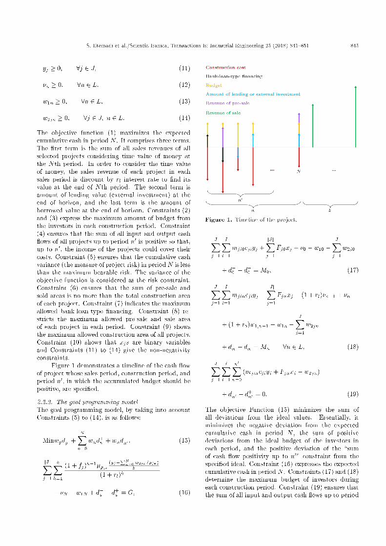
The objective function (1) maximizes the expectedcumulative cash in period N . It comprises three terms.The �rst term is the sum of all sales revenues of allselected projects considering time value of money atthe Nth period. In order to consider the time valueof money, the sales revenue of each project in eachsales period is discount by rl interest rate to �nd itsvalue at the end of Nth period. The second term isamount of lending value (external investment) at theend of horizon, and the last term is the amount ofborrowed value at the end of horizon. Constraints (2)and (3) express the maximum amount of budget fromthe investors in each construction period. Constraint(4) ensures that the sum of all input and output cash ows of all projects up to period n0 is positive so that,up to n0, the income of the projects could cover theircosts. Constraint (5) ensures that the cumulative cashvariance (the measure of project risk) in periodN is lessthan the maximum bearable risk. The variance of theobjective function is considered as the risk constraint.Constraint (6) ensures that the sum of pre-sale andsold areas is no more than the total construction areaof each project. Constraint (7) indicates the maximumallowed bank-loan-type �nancing. Constraint (8) re-stricts the maximum allowed pre-sale and sale areaof each project in each period. Constraint (9) showsthe maximum allowed construction area of all projects.Constraint (10) shows that xjs are binary variablesand Constraints (11) to (14) give the non-negativityconstraints.

Figure 1 demonstrates a timeline of the cash owof project whose sales period, construction period, andperiod n0, in which the accumulated budget should bepositive, are speci�ed.

2.2.2. The goal programming modelThe goal programming model, by taking into accountConstraints (5) to (14), is as follows:

Minwgd�g +NXn=0

wnd+n + wnd+

n0 ; (15)

jJjXj=1

kXh=1

(1 + fj)h�1�pjs(yj�PN

n=0 w2jn=pjn)k

(1 + rl)h

+ �N � w1N + d�g � d+g = G; (16)

Figure 1. Timeline of the project.

jJjXj=1

jIjXi=1

mji0cjiyj +jJjXj=1

Fj0xj + �0 � w10 �jJjXj=1

w2j0

+ d�0 � d+0 = M0; (17)

jJjXj=1

jIjXi=1

mjincjiyj +jJjXj=1

Fjnxj � (1 + rl)�n�1 + �n

+ (1 + rb)w1;n�1 � w1n �jJjXj=1

w2jn

+ d�n � d+n = Mn 8n 2 L; (18)

jJjXj=1

jIjXi=1

n0Xn=0

(mjincjiyj + Fjnxj � w2jn)

+ d�n0 � d+n0 = 0: (19)

The objective Function (15) minimizes the sum ofall deviations from the ideal values. Essentially, itminimizes the negative deviation from the expectedcumulative cash in period N , the sum of positivedeviations from the ideal budget of the investors ineach period, and the positive deviation of the \sumof cash ow positivity up to n0" constraint from thespeci�ed ideal. Constraint (16) expresses the expectedcumulative cash in period N . Constraints (17) and (18)determine the maximum budget of investors duringeach construction period. Constraint (19) ensures thatthe sum of all input and output cash ows up to period


n0 is positive so that the projects' income could covertheir costs up to n0.

3. Application of the model

To evaluate the performance of the proposed models,a set of 9 sample problems is designed. In addition,the weight of the objectives is measured through theFuzzy Analytic Hierarchy Process (FAHP). The single-objective model along with the goal-programmingmodel is solved using the ILOG CPLEX 12.1.

3.1. Data development and parameteradjustment

A set of 9 sample problems with time horizon belongingto f8; 9; 10g periods and 10, 15, and 20 projects isdesigned. The corresponding values of parameters arereported in Table 1.

The mean building sale price in ation is calcu-lated based on the geometric mean Eq. (20) in whicha1 and aN are the sale prices in the �rst and Nthperiods, respectively. Di�erent sale price in ation ratesare assigned to di�erent projects based on the place'sgrowth potential (see Table 1):

f = N

raNa1� 1 = 0:054: (20)

All building sale prices for di�erent years are in atedwith a 0.054 in ation rate and transferred to the �nalperiod. In order to calculate the mean building saleprice and the building sale price variance, Eqs. (21)and (22) are utilized:

�pjs =n=NXn=1

an(1 + f)N�nN

= 83:037; (21)

�2pjs =

Pn=Nn=1 (�n(1 + f)N�n � �pjs)2

N � 1= 276:475:

(22)

The parameters such as fj , interest rates, B1n, pjn,�pjs, and �pjs are determined based on market andbank situations; numbers of construction and saleperiod are determined based on real situations ofthe construction company. Through a variety ofconstruction projects, the exact and speci�c data forother parameters, such as Kj , �xed and variablecosts, are not available because of the poor accountingmethods, but the ranges for each of them are calculatedaccording to the rough estimates. We use severaldata by considering random distribution around thecalculated parameter to assess validation of the modeland evaluate whether the output is in uenced by aspeci�c data or not.

Since risk of investments can be evaluated byestimating standard deviations of net cash ows foreach alternative investment and such a measure ismore precisely de�ned as a statistical measure of un-certainty [35,36], therefore, in this paper, the projects'risk is considered in the same way. Moreover, becausethe exact value of the risk upper bound (p) is notavailable, one can solve the single-objective modelthrough eliminating the risk (the more pro�table theproject, the higher the risk or the variance), and thenplace all parameters and obtained variables in therisk constraint and calculate the maximum value forit. Thereafter, based on the company's policy andits risk-taking level, one can adjust an upper-boundrisk constraint equal to a proportion of the maximumcalculated value (e.g., 0.0, 0.3, 0.5, 0.8, etc.). Thesingle-objective model considering the risk constraintis solved, whose optimal value and associated risk areconsidered as the ideal and the upper-bound risk con-straints in the goal programming model, respectively.

3.2. Objectives' weight in the goalprogramming model

In order to run the Fuzzy Analytic Hierarchy Process(FAHP) and determine the weights of the introduced

Table 1. Values of common parameters in sample problems.

Parameters Valuesk 4r 4rl 0.05rb 0.0625�jn 0.5B1n 80% of the sum of Mn up to that periodmjin A random value from (0-2)kj A random value from (10,000-15,000) square meterfj A random value from (0.027-0.081)�pjs A random value from (38-80)cji e.g., jIj = 4, A random value from (0.1-0.3), (0.3-0.5), (0.5-0.7), (0.7-0.9)Mn A random value from (50000-70000), e.g. 52,910


Table 2. Fuzzy numbers for pairwise comparisons.

Equal preference (1, 1, 1)Medium preference (1/2, 1, 3/2)Strong preference (1, 3/2, 2)

Very strong preference (3/2, 2, 5/2)Absolute preference (2, 5/2, 3)

objectives in the proposed model, the extent analysismethod [19] is used. The applied fuzzy numbers [37]are given in Table 2. Pairwise comparisons between theobjectives are based on the decision-maker's opinions(Weight 1 in Table 3). Other weights in Table 3 areobtained according to sensitivity analysis performed ondi�erent weights.

3.3. Application of the single-objective andgoal programming models

The exact solutions of the single-objective and goal-programming models are obtained using the ILOGCPLEX 12.1 software, which is capable of solvingquadratic problems. The CPLEX running time variesfrom a few hundredth of a second to a few seconds. Thesolution procedure seems reasonable since the capitalbudgeting problem is in the category of the strategicproblems and time is not a matter of concern.

The output of the single-objective model deter-mines the projects that own the cumulative cash at theend of the time horizon, construction area, and pre-saleand sale amounts of each project for each period. Also,the amount of money borrowed and lent for externalinvestment is determined. A project is not selected if itis not pro�table enough. In other words, its pro�t is lessthan that from the external investment. The lendingand borrowing activities cannot occur simultaneouslyin the same period.

The set of problems with 0.0, 0.3, 0.5, and 0.8risk coe�cients is solved. Any decrease in the riskcoe�cient decreases the amounts of sale and increasesthe amounts of pre-sale, while the pro�t at the end ofthe time horizon decreases. A risk coe�cient equal to

0.0 results in the pre-sale of all the selected projectsand the amounts of their sale remains zero.

In problems with similar projects, increasing thenumber of construction periods in order to cover thecosts leads to an increase in the amount of pre-sale anda decrease in the amounts of sale. In some cases, anyincrement in the number of construction periods mightcause the project to become unpro�table. If none ofthe projects is pro�table under any circumstances, theexternal investment option becomes preferable.

4. Analysis and discussion

In this section, the sensitivity analysis of both single-objective and goal-programming models is discussed.

4.1. Sensitivity analysis of the parameters ofthe single-objective model

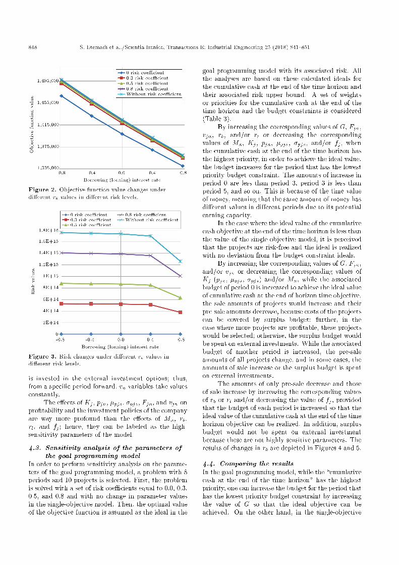
By increasing the corresponding values of Fjn, vjn,rb, and or rl up to the point that the risk becomeszero, the values of the objective function decreasebecause the expenditure is more than the revenueof projects; moreover, the risk parameter decreasesbecause the amounts of pre-sale to cover the costsincrease. Increasing the values of Mn, Kj , pjn, �pjs,�pjs, and/or fj will increase the corresponding valuesof the objective function and risk parameter (the morepro�table the project, the higher its risk). As anexample, the results of changing the values of rb onobjective function values in Figure 2 and on risk valuesare depicted in Figure 3.

4.2. External investment analysis underdi�erent parameter values in thesingle-objective model

Decreasing the corresponding values of Kj , pjn, �pjs,and �pjs and increasing the corresponding values ofFjn, and vjn show that, at a point of change, all theprojects become unpro�table, or a smaller number ofthem remain in the pro�tability zone, while this causesall or parts of the available budget to stay untouched.In this case, all or a portion of the unused budget

Table 3. Set of 4 weights for the 8 periods time horizon problem.

Objectives Weight 1 Weight 2 Weight 3 Weight 4

Cumulative cash at the end of the time horizon 0.16563 0.16563 0.16563 0.16563Budget constraint of period 0 0.15234 0.03790 0.15234 0.15234Budget constraint of period 1 0.13921 0.06200 0.13921 0.13921Budget constraint of period 2 0.12587 0.09044 0.12587 0.12587Budget constraint of period 3 0.11672 0.10988 0.03790 0.11672Budget constraint of period 4 0.10988 0.11672 0.10988 0.10988Budget constraint of period 5 0.09044 0.12587 0.09044 0.03790Budget constraint of period 6 0.06200 0.13921 0.06200 0.06200Budget constraint of period 7 0.03790 0.15234 0.11672 0.09044


Figure 2. Objective function value changes underdi�erent rb values in di�erent risk levels.

Figure 3. Risk changes under di�erent rb values indi�erent risk levels.

is invested in the external investment options; thus,from a speci�c period forward, vn variables take valuesconstantly.

The e�ects of Kj , pjn, �pjs, �pjs, Fjn, and vjn onpro�tability and the investment policies of the companyare way more profound than the e�ects of Mn, rb,rl, and fj ; hence, they can be labeled as the high-sensitivity parameters of the model.

4.3. Sensitivity analysis of the parameters ofthe goal programming model

In order to perform sensitivity analysis on the parame-ters of the goal programming model, a problem with 8periods and 10 projects is selected. First, the problemis solved with a set of risk coe�cients equal to 0.0, 0.3,0.5, and 0.8 and with no change in parameter valuesin the single-objective model. Then, the optimal valueof the objective function is assumed as the ideal in the

goal programming model with its associated risk. Allthe analyses are based on these calculated ideals forthe cumulative cash at the end of the time horizon andtheir associated risk upper bound. A set of weightsor priorities for the cumulative cash at the end of thetime horizon and the budget constraints is considered(Table 3).

By increasing the corresponding values of G, Fjn,vjn, rb, and/or rl or decreasing the correspondingvalues of Mn, Kj , pjn, �pjs, �pjs, and/or fj , whenthe cumulative cash at the end of the time horizon hasthe highest priority, in order to achieve the ideal value,the budget increases for the period that has the lowestpriority budget constraint. The amounts of increase inperiod 0 are less than period 3, period 3 is less thanperiod 5, and so on. This is because of the time valueof money, meaning that the same amount of money hasdi�erent values in di�erent periods due to its potentialearning capacity.

In the case where the ideal value of the cumulativecash objective at the end of the time horizon is less thanthe value of the single-objective model, it is perceivedthat the projects are risk-free and the ideal is realizedwith no deviation from the budget constraint ideals.

By increasing the corresponding values of G, Fjn,and/or vjn or decreasing the corresponding values ofKj (pjn, �pjs, �pjs) and/or Mn, while the associatedbudget of period 0 is increased to achieve the ideal valueof cumulative cash at the end of horizon time objective,the sale amounts of projects would increase and theirpre-sale amounts decrease, because costs of the projectscan be covered by surplus budget; further, in thecase where more projects are pro�table, these projectswould be selected; otherwise, the surplus budget wouldbe spent on external investments. While the associatedbudget of another period is increased, the pre-saleamounts of all projects change, and in some cases, theamounts of sale increase or the surplus budget is spenton external investments.

The amounts of only pre-sale decrease and thoseof sale increase by increasing the corresponding valuesof rb or rl and/or decreasing the value of fj , providedthat the budget of each period is increased so that theideal value of the cumulative cash at the end of the timehorizon objective can be realized. In addition, surplusbudget would not be spent on external investmentbecause these are not highly sensitive parameters. Theresults of changes in rb are depicted in Figures 4 and 5.

4.4. Comparing the resultsIn the goal-programming model, while the \cumulativecash at the end of the time horizon" has the highestpriority, one can increase the budget for the period thathas the lowest priority budget constraint by increasingthe value of G so that the ideal objective can beachieved. On the other hand, in the single-objective


Figure 4. Increase in each period's budget to realize G(with the increase in rb); a 0.5 risk coe�cient.

model, any deviation from the budget constraints forthe purpose of achieving more pro�t is not possible,because they are considered as hard constraints. Infact, it is possible that the companies' favorable pro�tlevel is higher than the calculated value in the single-objective model, and the company is able, to someextent, to increase the budget of each period. In thiscase, the single-objective model does not su�ce and

Figure 6. Comparing the results of the single-objectiveand goal programming models with the increase in G; a0.5 risk coe�cient.

the goal programming model is suitable to reach thespeci�ed pro�t level (Figure 6).

5. Conclusions

In this research, the capital budgeting problem for thecase of a construction company is modeled. Consid-

Figure 5. Increase in each period's budget to realize G (with the increase in rb) in di�erent risk levels.


ering the time value of money and di�erent �nancialresources with di�erent interest rates in the modelingis of great importance, which is one of the advantagesof the presented models in this paper.

Since the real-world budget constraints are soft,goal programming is used to model the problem. Infact, in the goal programming model, one can modifythe cumulative cash at the end of the time horizon tobe set equal to the company's favorable value, so thatthe surplus budget of each period can be assigned andthe speci�ed ideal achieved. In this research, the FAHPapproach is utilized and the risk of the projects is takeninto account. The exact solutions of the models areobtained using the ILOG CPLEX.

The sensitivity analysis for both models is per-formed. Parameters, including pre-sale prices, meanand variance of the sale price, �xed and variableconstruction costs, and maximum allowed area underconstruction of the project, are among the highlysensitive parameters, meaning that any change in theseparameters would a�ect the whole investment policyof the company. In addition, a change in theseparameters, in some cases, increases the possibility ofthese projects to become unpro�table, while makingthe external investment a better option.

Since no particular model is presented for cap-ital budgeting in the construction industry and thepresented model in this article is based on the realcircumstances of construction companies, it helps theconstruction companies in many ways, such as �nancialplanning, selection of optimal investment opportuni-ties, and choosing �nancial resources. Furthermore,the presented model considers the risk parameter as aconstraint; therefore, the pro�t calculation at the endof the time horizon becomes more realistic.

A future research direction is modeling the prob-lem such that features, such as the building char-acteristics and their quality levels, are added. Fur-ther, pre-sale prices and construction costs can beconsidered uncertain. Further, the uncertainty or riskminimization can be considered as an objective in thegoal programming model, and one can consider specialdistribution function for the amount of selling at eachsales period.

References

1. Famakin, I.O. and Saka, N. \Evaluation of the capitalbudget planning practice of contractors in the con-struction industry", Journal of Building Performance,2(1), pp. 26-32 (2011).

2. Mutti, C.D.N. and Hughes, W. \Cash ow manage-ment in construction �rms", Presented at 18th AnnualARCOM. Conf., Association of Researchers in Con-struction Management, University of Northumbria, 1,pp. 23-32 (2002).

3. Aziz, R.F. \Optimizing strategy for repetitive con-struction projects within multi-mode resources",Alexandria Engineering Journal, 52(1), pp. 67-81(2013).

4. Zhang, Q., Huang, X., and Tang, L. \Optimal multi-national capital budgeting under uncertainty", Com-puters & Mathematics with Applications, 62(12), pp.4557-4567 (2011).

5. Periasamy, P., A Textbook of Financial Cost andManagement Accounting, Himalaya Publishing House(2010).

6. Lorie, J.H. and Savage L.J. \Three problems in ra-tioning capital", The Journal of Business, 28(4), pp.229-239 (1955).

7. Weingartner, H.M., Mathematical Programming andthe Analysis of Capital Budgeting Problems, Engle-wood Cli�s. N. J.:Prentice-Hall, Inc (1963).

8. Park, C.S. and Sharp-Bette, G.P., Advanced Engineer-ing Economics, New York: Wiley (1990).

9. Weingartner, H.M. \Capital rationing: An authors insearch of a plot", The Journal of Finance, 32(5), pp.1403-1431 (1977).

10. Taylor, B.W. and Keown, A.J. \A mixed-integer goalprogramming model for capital budgeting within a po-lice department", Computers, Environment and UrbanSystem, 6(4), pp. 171-181 (1981).

11. Lawrence, K.D. and Reeves, G.R. \A zero-one goalprogramming model for capital budgeting in a prop-erty and liability insurance company", Computers &Operations Research, 9(4), pp. 303-309 (1982).

12. Mukherjee, K. and Bera, A. \Application of goalprogramming in project selection decision - A casestudy from the Indian coal mining industry", EuropeanJournal of Operational Research, 82(1), pp. 18-25(1995).

13. Thizy, J.M., Pissarides, S., Rawat, S., and Lane,D.E., Interactive Multiple Criteria Optimization forCapital Budgeting in a Canadian TelecommunicationsCompany, Springer Berlin Heidelberg, pp. 128-147(1996).

14. Badri, M.A., Davis, D., and Davis, D. \A comprehen-sive 0-1 goal programming model for project selection",International Journal of Project Management, 19(4),pp. 243-252 (2001).

15. Vashishth, T.K., Babu, G.R., and Singh, R.K. \Cap-ital Budgeting In Hospitals-A Case Study", Inter-national Journal of Advanced Research in ComputerScience and Software Engineering, 2(6), pp. 87-92(2012).

16. Ghosh D. and Roy, S. \A decision-making frameworkfor process plant maintenance", European Journal ofIndustrial Engineering, 4(1), pp. 78-98 (2010).

17. Badri, M.A. \Combining the analytic hierarchy processand goal programming for global facility location-allocation problem", International Journal of Produc-tion Economics, 62(3), pp. 237-248 (1999).


18. Ribeiro, R.A. \Fuzzy multiple attribute decision mak-ing: a review and new preference elicitation tech-niques", Fuzzy Sets and Systems, 78(2), pp. 155-181(1996).

19. Chang, D.Y. \Applications of the extent analysismethod on fuzzy AHP", European Journal of Oper-ational Research, 95(3), pp. 649-655 (1996).

20. Chaghooshi, A., Arab, A., and Dehshiri, S. \A fuzzyhybrid approach for project manager selection", Deci-sion Science Letters, 5(3), pp. 447-460 (2016).

21. Rathi, R., Khanduja, D., and Sharma, S. \A fuzzyMADM approach for project selection: a six sigmacase study", Decision Science Letters, 5(2), pp. 255-268 (2016).

22. Ghazimoradi, M., Kheyroddin, A., and Rezayfar, O.\Diagnosing the success of the construction projectsduring the initial phases", Decision Science Letters,5(3), pp. 395-406 (2016).

23. Tang, Y.C. and Chang, C.T. \Multicriteria decision-making based on goal programming and fuzzy analytichierarchy process: An application to capital budgetingproblem", Knowledge-Based Systems, 26, pp. 288-293(2012).

24. Ai, J. and Wang, T. \Enterprise Risk Managementand Capital Budgeting under Dependent Risks: AnIntegrated Framework", 2012 Enterprise Risk Manage-ment Symposium, April 18-20, pp. 1-6 (2012).

25. Cala�ore, G.C. \Multi-period portfolio optimizationwith linear control policies", Automatica, 44(10), pp.2463-2473 (2008).

26. Markowitz, H. \Portfolio selection", The Journal ofFinance, 7(1), pp. 77-91 (1952).

27. Lintner, J. \The valuation of risk assets and the selec-tion of risky investments in stock portfolios and capitalbudgets", The Review of Economics and Statistics,47(1), pp. 13-37 (1965).

28. Sharpe, W.F. \A linear programming algorithm formutual fund portfolio selection", Management Science,13(7), pp. 499-510 (1967).

29. Sharpe, W.F., Portfolio Theory and Capital Markets,New York: McGraw-Hill College (1970).

30. Linsmeier, T.J. and Pearson, N.D. \Risk measurement:An introduction to value at risk", Working paperUniversity of Illinois at Urbana-Champain (1996).

31. Su, X.L. and Huang, X.X. \Mean-variance model foroptimal multinational project adjustment and selec-tion", In Applied Mechanics and Materials, 380, pp.4809-4814, (2013).

32. Babaei, S., Sepehri, M.M., and Babaei, E. \Multi-objective portfolio optimization considering the depen-dence structure of asset returns", European Journal ofOperational Research, 244(2), pp. 525-539 (2015).

33. Beraldi, P., Violi, A., De Simone, F., Costabile, M.,Massab�o, I., and Russo, E. \A multistage stochasticprogramming approach for capital budgeting prob-lems under uncertainty", IMA Journal of ManagementMathematics, 24(1), pp. 89-110 (2013).

34. Khalili-Damghani, K. and Taghavifard, M. \Solving abi-objective project capital budgeting problem using afuzzy multi-dimensional knapsack", J. Ind. Eng. Int.,7(13), pp. 67-73 (2011).

35. Hillier, F.S. \The derivation of probabilistic informa-tion for the evaluation of risky investments", Manage-ment Science, 9(3), pp. 443-457 (1963).

36. Walls, M.R. \Combining decision analysis and portfo-lio management to improve project selection in the ex-ploration and production �rm", Journal of PetroleumScience and Engineering, 44(1), pp. 55-65 (2004).

37. Tolgaa, E., Demircana, M.L., and Kahraman, C.\Operating system selection using fuzzy replacementanalysis and analytic hierarchy process", InternationalJournal of Production Economics, 97(1), pp. 89-117(2005).

Biographies

Sepideh Etemadi received the BSc degree in Indus-trial Engineering from Bahonar University of Kermanand MSc degree in the same �eld from FerdowsiUniversity of Mashhad. Her research interests lie inthe project portfolio selection, capital budgeting andoptimization. She has presented papers in the 7thInternational Conference of Iranian operations researchsociety, 12th International Conference on IndustrialEngineering, and International Conference on Indus-trial Engineering and Management on these subjects.

Hamidreza Koosha received his BSc and MSc de-grees in Industrial Engineering from Sharif Univer-sity of Technology and his PhD degree in IndustrialEngineering from Tarbiat Modares University. He isan Assistant Professor in Industrial Engineering atFerdowsi University of Mashhad. His main researchinterests include Mathematical modeling and dataanalytics for customer relationship management andproject portfolio selection. His publications appear inbooks and journals such as Management Decision andJournal of modelling in management.

Majid Salari received the BSc and MSc degrees inApplied Mathematics from the Ferdowsi University ofMashhad, Iran in 2004 and 2006, respectively. Inaddition, he has PhD in Automations and OperationsResearch from the University of Bologna, Italy in2010. In 2010, he joined the Department of IndustrialEngineering, Ferdowsi University of Mashhad, as anAssistant Professor, and became an Associate Professorin 2016. His current research interests include com-binatorial optimization, applied operation research,evolutionary computation, heuristic search, logistics,distribution, and vehicle routing.

A goal programming capital budgeting model under...

Documents

Transcript of A goal programming capital budgeting model under...