Carnegie Mellon UniversityResearch Showcase @ CMU

Department of Chemical Engineering Carnegie Institute of Technology

1992

A global optimization algorithm for heat exchangernetworksIgnacio QuesadaCarnegie Mellon University

Ignacio E. Grossmann

Carnegie Mellon University.Engineering Design Research Center.

Follow this and additional works at: http://repository.cmu.edu/cheme

This Technical Report is brought to you for free and open access by the Carnegie Institute of Technology at Research Showcase @ CMU. It has beenaccepted for inclusion in Department of Chemical Engineering by an authorized administrator of Research Showcase @ CMU. For more information,please contact research-showcase@andrew.cmu.edu.

NOTICE WARNING CONCERNING COPYRIGHT RESTRICTIONS:The copyright law of the United States (title 17, U.S. Code) governs the makingof photocopies or other reproductions of copyrighted material. Any copying of thisdocument without permission of its author may be prohibited by law.

A Global Optimization Algorithmfor Heat Exchanger Networks

I. Quesada, I.E. Grossmann

EDRC 06-138-92

A Global Optimization Algorithm

for Heat Exchanger Networks

Ignacio Quesada and Ignacio E. Grossmann*Department of Chemical Engineering

Carnegie Mellon UniversityPittsburgh. PA 15213

May 1992

* Author to whom correspondence should be addressed

Abstract

This paper deals with the global optimization of heat exchanger networks with fixed topology.

It is shown that if linear area cost functions are assumed, as well as arithmetic mean driving

force temperature differences in networks with isothermal mixing, the corresponding NLP

optimization problem involves linear constraints and linear rational functions in the

objective which are nonconvex. A rigorous algorithm is proposed that is based on a convex

NLP underestimator that involves linear and nonlinear estimators for rational and bilinear

terms which provide a tight lower bound to the global optimum. This NLP problem is used

within a spatial branch and bound method for which branching rules are given. Basic

properties of the proposed method are presented, and its application is illustrated with several

example problems. The results show that the proposed method only requires few nodes in the

branch and bound search.

Mathematical model

Two major simplifications have been assumed in the optimization model of heat exchanger

networks that provide a mathematical structure that can be exploited for the global

optimization. The area cost is given by a linear function and the driving force for the heat

exchangers is calculated by the arithmetic mean temperature difference at both ends of the

heat exchanger.

For a given heat exchanger network (HEN) configuration consisting of n exchangers of

which the subset EU are utilities, the mathematical formulation can be stated as a linearly

constrained NLP problem of the following form:

sL g(Q.AT.x)£O (P)

X€X

T^ATtSATjU i=l n

where Qt corresponds to the heat load of the heat exchanger i and AT, is the driving force for the

heat exchanger; His the heat transfer coefficient, q is the area cost coefficient and d* the utility

cost The lower bounds for the driving forces, ATtL, are strictly positive since fixed network

configurations are considered and they have to be greater or equal than a minimum exchanger

approach temperature, EMAT. The heat loads Q are nonnegattve, although valid finite lower

and upper bounds as is the case for ATt can be obtained by preanalysis of a given network

structure. The variables x are all the additional variables in the formulation (Le. intermediate

temperatures). The function g involves a set of linear constraints that describe networks that

can be embedded in the superstructure of Yee and Grossmann (1991) in which isothermal

mixing of streams is assumed. These constraints include heat balances, definition of driving

forces and approach temperature constraints. An example of problem (P) is given later in the

paper (model (PEX)).

The difficulty in solving problem (P) lies in the fact that it has a nonconvex objective

function that can have multiple local minima. Furthermore, these local solutions will not

necessarily correspond to extreme points of the feasible region since the objective function is

the sum of linear fractional functions. Each of these functions is pseudolinear (pseudoconvex

and pseudoconcave), which means that they can project either as monotonically increasing or

monotonlcally decreasing functions. In this way the complete objective function is neither

convex nor concave and the local solutions can be extreme or non extreme points (

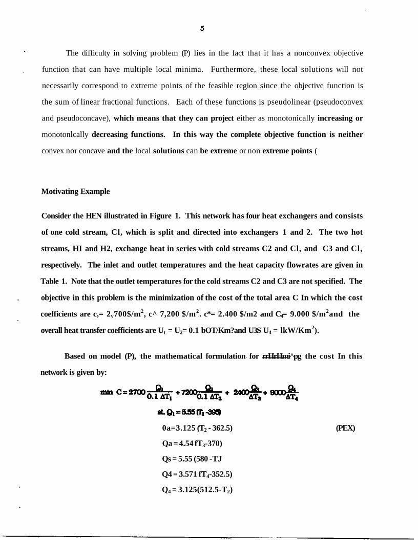
Motivating Example

Consider the HEN illustrated in Figure 1. This network has four heat exchangers and consists

of one cold stream, Cl, which is split and directed into exchangers 1 and 2. The two hot

streams, HI and H2, exchange heat in series with cold streams C2 and Cl, and C3 and Cl,

respectively. The inlet and outlet temperatures and the heat capacity flowrates are given in

Table 1. Note that the outlet temperatures for the cold streams C2 and C3 are not specified. The

objective in this problem is the minimization of the cost of the total area C In which the cost

coefficients are c,= 2v700$/m2, c^ 7,200 $/m2. c*= 2.400 $/m2 and C4= 9.000 $/m2and the

overall heat transfer coefficients are Ut = U2= 0.1 bOT/Km?and U3S U4 = lkW/Km2).

Based on model (P), the mathematical formulation for rrHrHmi pg the cost In this

network is given by:

0a=3.125 (T2 - 362.5) (PEX)

Qa = 4.54 fT3-370)

Qs = 5.55 (580 -TJ

Q4 = 3.571 fT4-352.5)

Q4 = 3.125(512.5-T2)

Tj >400 + 5

T3>400 + 5

Qi +02=100

Ti - 305

T2 - 302AT2 = 2

T t - T3+210AT3= g

T2 - T4 + 360AT4=-Jfc =5

395<T!<575

398<T2<718

365<£T3

358 <T4

in which a value of EMAT = 5 (minimum exchanger approach temperature) has been assumed.

Since the problem has a total of 12 variables and 11 independent equations it has one degree of

freedom. Figure 2 shows the objective function of this formulation, the total area cost of the

network, plotted against Qi, the heat load of the first heat exchanger. The feasible region for

the network, Qi € [ 5.55, 97.81], is defined by the minimum approach temperature constraints.

As it can be seen in Fig. 2 there are two local optimal solutions. The first local solution with

cost O$ 45,687 is located in the convex portion of the projection of the objective function and

it corresponds to the interior point Qi= 16.84 kW with a total area of 9.351 m2. The second

local solution with cost C=$36,160 corresponds to the global optimum. It lies at an extreme

point in the concave part and is defined by the approach temperature constraint of heat

exchanger 2; it is located at Qi = 97.812 kW with a total area of 9.254 m2. When a local search

technique is used for solving this problem, the solution will depend of the initial point that is

given. The next sections will develop a solution method that will rigorously determine the

global optimum for this problem regardless of the initial point that is selected.

Underestimator and overestimator functions

Problem (P) can be reformulated by introducing the variables A for the scaled areas (the

product of the area and the overall heat transfer coefficient) of the exchangers, and extra

constraints to relate each of these to its heat load and driving force. This yields the following

problem formulation.

i=l n

,£T,x)<0 (PI)

xeX

where A, = {Q,L£ Qt < Qxv. ATt

L < ATt < ATtu AL A A13}. 1=1 n

In problem (P) the nonconvexitles appear in the form of bilinear terms in the

constraints. In order to develop a valid lower bound to the global optimum, the nonconvex

terms in (PI) can be replaced by the linear overestimating functions proposed by McCormick

(1983) (see Appendix A eq A4). These functions can be expressed by the set of two inequalities

for each exchanger U i=l-..n,

AAT1£ALATi + AAT1u-A,LAT,u (1)

A AT, £ AuATt «• A AT,L - A u AT,L (2)

The above inequalities can be used to replace the bilinear terms in (PI) yielding an LP

underestimator problem. However, the predicted bounds by this problem are often not very

tight For this reason a new set of nonlinear convex underestimator functions are proposed

that can be generated from the original formulation (P) over the linear fractional terms of the

objective function (see Appendix A eq A14). Expressing the proposed nonlinear

underestimators in the form of inequalities yields:

AT, A T , u + W i n A T , AT,U

8

<<»

The following mathematical properties can be established between the linear and

nonlinear estimator functions in (1) and (2) and (3) and (4).

QL QUProperty 1: When A^ ^J-JJ (or A^ r c ) the linear overestimator (1) (or (2)) is a linearization

of the nonlinear underestimator (3) (or (4)).

Proof Consider the linear overestimator (1) and the area constraint form (PI),

&£ AMTt+AAT^-A^AT,11 (5)

Rearranging (5) leads to:

Using the condition that A^ Jj^j > equation (6) yields

' A T "AT,"

The nonlinear underestimator (3) gives rise to the constraint

The first term of equations (7) and (8) are the same. Now compare the term fr^f - AT ul trom

1 ATTthe nonlinear underestimator (8) with the term (—u ' #ATui 2 ) from t h e linear equation (7).

Both terms are equal at ATtu. Furthermore, a linearization of the nonlinear term of (8) at AT,=

ATtu yields the linear term:

Thus, (3) is a linearization of (1)

Corollary 1. The nonlinear underestimator (3) (or (4)) is stronger than the linear overestimator

(1) (or (2)) when A^ ^j (or Au=

Proof. From Property 1 and the fact that the nonlinear underestimators in (3) and (4) are

convex in ATlf any linearization is smaller or equal than the function ( see Fig. 3).

•

The following property, however, establishes that the linear overestimators in (1) and

(2) are not necessarily redundant

QL QUProperty 2. When A|L > ~JJ (or A^ < -~rc ) there is a part of the feasible region in which the

linear overestimator (1) (or (2)) is stronger than the nonlinear underestimator (3) (or (4)).

Proof. Consider a feasible point in A, such that ^7 = A^. with Qi* > QtL and ATt* <

Evaluating the linear overestimator (1) at (Qt+, AT,+) yields:

Then the linear overestimator for that point reduces to,

A, *AL (11)

The nonlinear underestimator (3) for this point is,

1 1 .

and using the relation 7 = AtLt for expressing (12) in terms of A^ yields.

Define a s - ^ j and p= -§p-. the equation (13) can be expressed as.

(14)

StaceO£a< 1 andO£p< 1

l=a+( l -a)>a+p( l -a) =• (15)

then the nonlinear underestimator reduces to

10

l (16)

Hence, the linear overestlmator (1) is stronger at the point (Qt\ AT ). B

In a similar way that nonlinear underestimator functions are used to obtain a convexQ

approximation for the terms Aj = -^r , underestimating functions can be generated for the

terms ATt > ,

< - ^ . ,17,

However, In this case the limitation is that (17) and (18) are only defined for the case when the

lower bound Af is greater than zero.

Geometrical Interpretation

The underestimator and overestimator functions (1) - (4) presented In the previous section have

the property that they match exactly the original function at the boundary of the feasible

region Ax of problem (PI) (see Appendix B for a proof). The fact that these estimator functions

are nonredundant over the feasible region can be interpreted geometrically in a 2-dimensional

diagram (see Figure 4). For a particular heat exchanger It Is possible to represent its feasible

region At in a 2-dimensional figure by plotting its driving force versus its heat load. In this

diagram the area of the heat exchanger Is given by the straight lines that pass through the

origin and have a positive slope. The nonlinear underestimators (3) and (4) provide an exact

approximation along the boundaries defined by the lower and upper bounds for the heat load,

Q, and the driving force, AT. The linear underestimators (1) and (2) provide an exact

approximation at the lower and upper bounds for the area. A, and the driving force, AT. In theQL QU

case that AL = TSrjJ (°r Au = T^T) the line that defines this boundary does not cut any part of

the feasible region that Is already defined by the bounds of the heat load and the driving force

resulting In a redundant linear overestlmator. When this is not the case, then there exists a

part of the feasible region in which the bound of the area Is stronger than the boundaries

11

determined by the bounds of the heat load and driving force (see Fig. 4). At these boundaries

(AL. Au), the linear overestimators provide an exact representation of the original functions

while the nonlinear underestimators give a weaker approximation. In this way both

estimators complement each other in the approximation of the fractional terms.

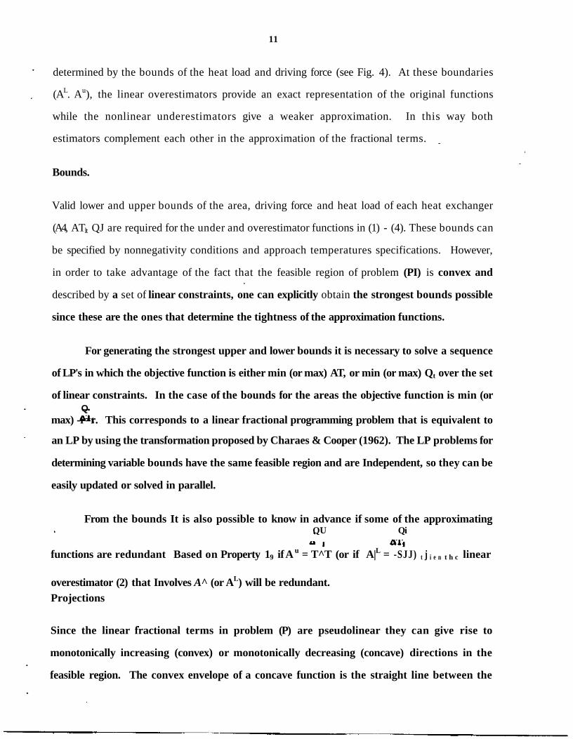
Bounds.

Valid lower and upper bounds of the area, driving force and heat load of each heat exchanger

(A4, ATlt QJ are required for the under and overestimator functions in (1) - (4). These bounds can

be specified by nonnegativity conditions and approach temperatures specifications. However,

in order to take advantage of the fact that the feasible region of problem (PI) is convex and

described by a set of linear constraints, one can explicitly obtain the strongest bounds possible

since these are the ones that determine the tightness of the approximation functions.

For generating the strongest upper and lower bounds it is necessary to solve a sequence

of LP's in which the objective function is either min (or max) AT, or min (or max) Qt over the set

of linear constraints. In the case of the bounds for the areas the objective function is min (orQ

max) -r=r. This corresponds to a linear fractional programming problem that is equivalent to

an LP by using the transformation proposed by Charaes & Cooper (1962). The LP problems for

determining variable bounds have the same feasible region and are Independent, so they can be

easily updated or solved in parallel.

From the bounds It is also possible to know in advance if some of the approximatingQU Qi

functions are redundant Based on Property 19 if Au = T^T (or if A|L = -SJJ) t j i e n t h c linear

overestimator (2) that Involves A^ (or AL) will be redundant.Projections

Since the linear fractional terms in problem (P) are pseudolinear they can give rise to

monotonically increasing (convex) or monotonically decreasing (concave) directions in the

feasible region. The convex envelope of a concave function is the straight line between the

12

extreme points. In the case of a convex function, its convex envelope is the function itself. In

the 2-dimensional diagram of the feasible region of a particular heat exchanger, there are both

concave and convex directions of the fractional term defining the area of that heat exchanger.

It is easy to show that the straight lines with positive slope represent the concave directions,

while the straight lines with a negative slope correspond to the convex directions (see Fig. 5).

Specifically, let

ATj = a + bQt (19)

Then for At £ ~r •

(20)

the right hand side of (20) has a positive second derivative for b < 0 (see also Property 3 later in

this paper).

Since the nonlinear underestfmator and linear overestimator functions (l)-(4) do not

provide exact approximations in convex directions such as the ones shown in Fig 5, It is

possible to develop exact nonlinear underestimators in the convex directions. These are

obtained by expressing the lower and/or upper bounds of one variable as a function of the other

variable involved in the estimator. In this case it is necessary to ensure that this nonlinear

functionality does not destroy the convexity of the approximating function*

The proposed underestimator described above corresponds to a projection along the

convex direction. As shown below, this projection can be obtained without any extra cost when

bounds are generated for the variables in the approximating functions since the Lagrange

multipliers of the bounding subproblems can be used to generate this projection.

Consider the case that the upper bound (equivalent for the lower bound) of the driving

force AT,of a given heat exchanger is projected over its respective heat load Qt(in a similar way

projections can be obtained for the heat load over its driving force).

13

min -ATt

Tx^<0 (P2)

A Benders cut for problem (P2) is given by:

-ATt ;> -ATt + ]£*, g j(Qt, AT,, x i (21)J

where Aj are the Lagrange multipliers and x* is the solution of all the remaining variables in the

LP problem in (P2). The above projection results in.

This is a linear function that can be expressed as,

AT,<a + b& (23)

This function has to have a negative slope (b < 0) to represent a convex direction of the

objective function as was shown previously* Therefore, it is possible to generate an additional

convex nonlinear underestimator that Is nonredundant to the previous ones (see Property 3),

and it is given by:

a + bQi + e ^JL _____AT, * a + bQ, Tvrr"1 AT, " a + bQ,

Property 3 The nonlinear inequality (24) is a valid convex underestimator when b < O, and In

some part of the feasible region A, is stronger than the nonlinear underestimators (3) and (4),

EEBfiLFor the first part of the proof the constraint (23) can be expressed as:

AlT-iTbo;^0 (25>

Multiplying by the lower bound constraint for the heat load (Q, 2 Q{-) yields a the valid

inequalities:

( 2 6 )

14

Rearranging yields:

(27)

which correspond to the nonlinear underestimator (24).

The Hessian matrix of the underestimating function in (24) Is given by

2b(a+bQt1)

(a + bQO3

0

0

2 Q1

AT,3

The term (a+bQ,) is positive over all the feasible region since,

a+bQ, £ AT, > EMAT > 0

Also Q, £ 0, and therefore.

(28)

(29)

(Q,L> 0 if not the function reduces to just one convex term) (30)

and

2 b ( a + b<(a + b<

L>0 ifb<0 (31)

Therefore, If b<0 the Hessian matrix Is positive definitive and the function Is convex.

Now consider a feasible point In the strict Interior in A, such that AT,*= a + b Q, and AT,*

< AT,U. Equation (24) for the nonlinear underestimator with projection reduces to.

and therefore Is an exact approximation of the linear fractional term in (24). Since ATt+ does

not lie In the boundary of A, the nonlinear underestimator (3) yields.

ATt"

15

which is a strict inequality. Thus the underestimator (24) is stronger than the nonlinear

underestimator (3) in some part of the interior feasible region.

For the other underestimator (4) consider now a point such that Q,+ = (AT -a)/b and Qf <

Qtu, such a point exists since the projections are nonredundant constraints.

Equation (24) for the nonlinear underestimator with projection reduces to,

(34)a+bQ,*^"^1 AT, a+bQ,*' a+bQ,+ AT,

which is an exact approximation of the fractional term. The nonlinear underestimator (4)

yields,

h* ^^ 17< ATf

L y AAT tL ^ f ? AT,

which is an strict inequality.

Hence, there are parts of the feasible region where the projected underestimator (24) is stronger

than the nonlinear underestimator (4). •

It can happen that when the projection in (24) is obtained using the LP solution of

problem (P2), only a simple bound over the variable is obtained (i.e. b=O; a = AT,") instead of a

linear inequality. In this case it is possible to solve an additional problem fixing the

projection variable at a fixed value within the bounds (Le. Q, = Q,f with Q,L < Q,f < Q,").

The projected nonlinear underestimators in (24) are clearly useful when the feasible

region of a given heat exchanger has Interior faces with convex directions, since it is possible

to obtain exact approximations of this exchanger at these faces. The usefulness of these

underestimators will be shown with example 3 later in the paper.

In a similar way, projection terms can be generated for the lower bound of the driving

force with respect to its driving force and substituted in (4),

16

AT\ * a' + b'Q,

where a1 + b' Q, > AT,.

+ 9 ' U (AT, (36)

The projections that can be obtained for the bounds of the heat load in terms of its

driving forces are reduced to the same ones.

Convex nonlinear underestimator problem

Having derived a number of linear and nonlinear bounding approximations for the bilinear

and rational terms in (P) and (PI), a convex nonlinear underestimator problem (NLPJ for

problem (P) can be defined as follows. Valid bounds over the areas, driving forces and heat

loads are generated to define the set Q=uAit i=l..oi, and the nonconvexities of the original

problem are substituted by the convex approximating functions (1) - (4). (17), (18), (24) and (36).

The projections for the upper and lower bounds of the driving forces over Its heat load are given

by functions <KQi) = a+ bQt where the conditions of Property 3 are satisfied. The form of the

underestimator problem NLPLls the following:

nminCL-

(NLPJ

+ A, AT,U - A, »-ATiu

Q, S A,°AT, + A, AT,L -A u AT,L

1=1...n

WQt+ i=l...n for which 4> is a linear

of 0, with negative slope

17

X€X

(Q,AT.A)€fl

Property 4. Any feasible point (Q, AT, A, x) in problem NLPL provides a valid lower bound to the

objective function of problem (PI). Furthermore, the optimal solution CL* of (NLPJ provides a

valid lower bound to the global optimum (Cf) of problem (PI).

Proof. Any feasible point (Q, AT, A ,x) for problem (NLPJ is also a feasible solution to problem

(P) since the inequalities g(Q, AT, x) < 0 are satisfied in both problems. Since the approximating

functions in (NLPJ represent a relaxation of the bilinear Inequalities in (PI), they have the

effect of underestimating the objective function C of problem (PI). Thus it follows that at the

given feasible point CL £ C.

For the global optimum (Q\ AT, A\ x') of problem (PI) it then follows that Cf £ CL\ where

CL' is the objective of NLPL evaluated at that point. Since CL\ the optimal solution of NLPL is

unique due to its convexity. CL £ CL#f and thus C £ CL#. m

?n If the optimum solution CL# from NLPL is equal to the objective function value C

from (PI) it corresponds to the global optimum of (PI).

EEQQf If C is not the global optimal solution of problem (PI) then there exists a solution C# < C.

But by Property 4, Q,* £ C # which contradicts the assumption that Q > C Is a solution to NLPU

Partitioning Scheme p^fH1^1 ^w^ bound)

Problem NLPL will in general provide a tight lower bound to the original problem (PI).

However, since there will often be a gap between the lower bound CL from NLPL and the actual

objective function C, a spatial branch and bound search will be required to find the global

optimal solution. Corollary 2 provides a termination criteria to this search. In this section an

algorithm is presented that employs a partitioning scheme of the feasible region for the branch

and bound search.

18

During this search procedure, valid lower bounds C^k over subregions Qk and upper

bounds Cu of the global solution are generated. The lower bounds are provided by the solution

of convex underestimator problems NLPL over given subregions iik of the feasible space

(Property 4). Each subregion ftk is defined by a set of lower and upper bounds of the area, heat

load and driving force of the heat exchangers.

Any feasible solution of the set of original linear constraints clearly provides a valid

upper bound to the global solution of problem (P). Feasible solutions are obtained when the

bounds for the variables are calculated. Additionally the solution of the convex NLP

underestimator problem is a feasible solution. For all these points only an evaluation of the

original objective function is necessary to determine an upper bound. The best upper bound Cu

is stored as the incumbent solution C\

In some cases, it may prove to be useful to solve the original nonconvex problem (P)

with a given set of bounds (Qk) and a particular initial point (a solution of a convex

underestimator problem). This is mainly used in the case that the difference between the

convex underestimator CLk and the incumbent solution C* is small and the nonconvex problem

can help in adjusting the value of the variables, particularly if the objective function has only

small variations between local solutions.

When the lower bound CLk of a particular subregion Is greater or equal that the

incumbent solution C\ It Is an Indication that not further examination of this subregion Is

required. If a gap exists between the lower and upper bounds, the subregion Qk is divided Into

smaller subregions Qk+1 and Qk+2. so It Is possible to have tighter convex underestimator

problems. To divide the subregions it is necessary to select the nonconvex term corresponding

to a heat exchanger j over which the partition of the feasible region is made. This selection rule

Is based on the largest weighted difference between the exact value of the nonconvex term In OP)

and the convex approximation obtained by the solution of the convex underestimator problem

(see also Al-Khayyal and Falk (1983), Sherali and Alameddine (1990)). This rule is given by:

19

Rule 1.QiDetermine j e arg max1 [ q ( -r^r - Ajl as the nonconvex term over which partitioning is to be

performed.

The motivation for this criterion is to select the term for which the difference in the

approximation affects the most the value of the objective function, so that the existent gap can

be reduced by partitioning its corresponding region Aj.

A second selection rule, that is a variation of Rule 1, can be considered. In this rule a

parameter 8 e (O,1J is included and it defines a interval over which some candidate heat

exchangers are considered.

Rule2

Apply Rule 1 and set Uj

Defineie

Select j e Ik as the nonconvex term over which partitioning is to be performed.

When 6=1 this selection rule reduces to Rule 1. When &\ > lt a heat exchanger that has

not been previously used is selected. The advantage of this rule is that exchangers that have not

been previously selected can be partitioned and this allows for a tightening of their bounds as it

will be discussed later.

Once that the jth heat exchanger has been selected it is necessary to decide over which

variable Aj, Qj or AT,, the partitioning should be performed. It is possible to restrict the

algorithm to make partitions exclusively over the space of the areas, heat loads or driving

forces* although a combination of these may prove more useful. This aspect depends on how

interdependent are the bounds of the variables with respect to the partition variable. Once that

the variable bounds that define the partition of the feasible region are selected, an update in the

bounds of the other variables of that particular heat exchanger is done for each of the new

20

subregions. For these bounding problems the partition constraints that defined the subregion

are added to the linear constraints to provide tighter approximations.

In this work, the variable that is normally chosen for the partitions is the area Aj. In

case that exchanger j has been previously selected it is convenient to check if the bounds of the

driving force, AT,, and the heat load, Qjv were updated. If there was a change in these bounds

then the partition variable can remain the same. But if the bounds of a variable did not

change, then it is more efficient to choose it as the partition variable in this iteration. Also, in

cases where the bounds for the areas indicate that the linear overestimators are redundant it is

better to select the heat load or driving force over the area as the partition variable.

The value of the variable at which the partition is made correspond to the one of the

incumbent solution. Two subregions are created by the addition of the constraints:

Eitherz,<*zf or 3*z{ (37)

where z is either Aj, AT} or Qj depending on which variable was selected.

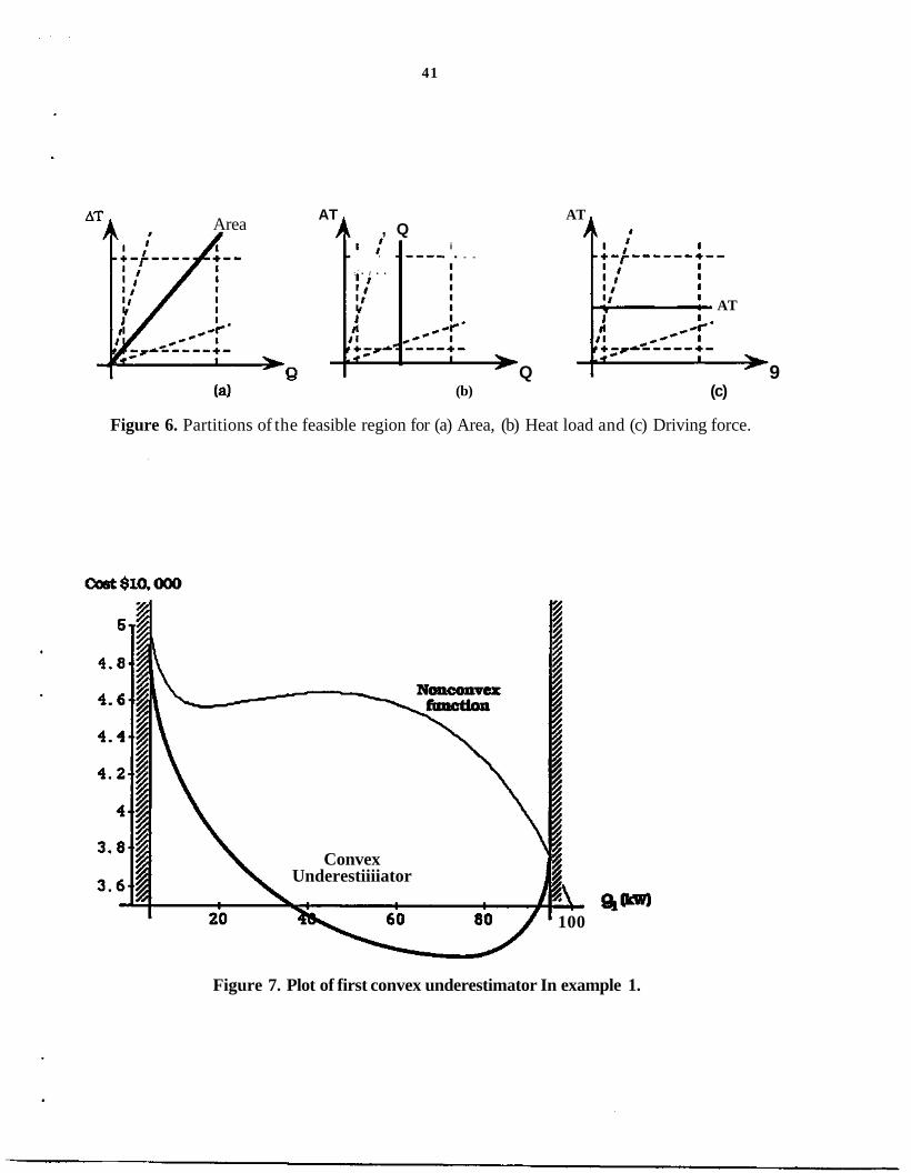
The partition scheme Is illustrated In Fig. 6.The divisions over the heat load and the

driving force correspond to rectangular partitions. The divisions over the area are partitions

of the feasible region in the nonconvex direction of the linear fractional term.

It can happen that the value of the partition variable in the incumbent solution is at

one of its bounds* In this situations a different variable of the exchanger j is considered as the

partition variable. If no variable (A,, ATj and Q) has a incumbent value that is not at a bound

then a different exchanger is selected for partition. When no variable can be selected for the

exchangers that do not have an exact approximation, then the value of the variables at the

solution of the convex subproblem is used for the partition constraints.

21

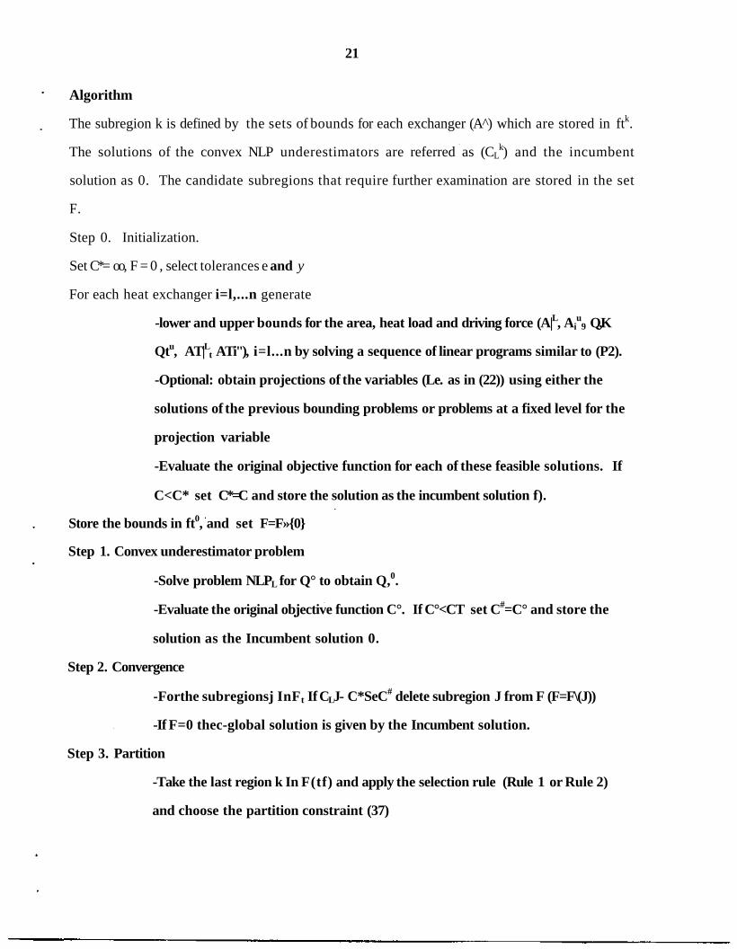
Algorithm

The subregion k is defined by the sets of bounds for each exchanger (A ) which are stored in ftk.

The solutions of the convex NLP underestimators are referred as (CLk) and the incumbent

solution as 0. The candidate subregions that require further examination are stored in the set

F.

Step 0. Initialization.

Set C*= oo, F = 0 , select tolerances e and y

For each heat exchanger i=l,...n generate

-lower and upper bounds for the area, heat load and driving force (A|L, Aiu

9 Q,K

Qtu, AT|Lt ATi"), i=l...n by solving a sequence of linear programs similar to (P2).

-Optional: obtain projections of the variables (Le. as in (22)) using either the

solutions of the previous bounding problems or problems at a fixed level for the

projection variable

-Evaluate the original objective function for each of these feasible solutions. If

C<C* set C*=C and store the solution as the incumbent solution f).

Store the bounds in ft0, and set F=F»{0}

Step 1. Convex underestimator problem

-Solve problem NLPL for Q° to obtain Q,0.

-Evaluate the original objective function C°. If C°<CT set C#=C° and store the

solution as the Incumbent solution 0.

Step 2. Convergence

-Forthe subregionsj InFt If CLJ- C*SeC# delete subregion J from F (F=F\(J))

-If F=0 thec-global solution is given by the Incumbent solution.

Step 3. Partition

-Take the last region k In F(tf) and apply the selection rule (Rule 1 or Rule 2)

and choose the partition constraint (37)

22

-Subdivide subregion Qk in subregions Qk+1 and Clk+2 by adding the respective

bound or inequality. Delete subregion Qk from F and store subregions Qk+1 and

ftk+2 in F (F=(F\{k}) u{k+l,k+2})

-Update the bounds in subregions k+1 and k+2 for the exchanger selected for the

partition.

Step 4. Convex underestimator problems

-Solve problem NLPL for ftk+1 and Qk*2 to obtain CLk+1 and CL

k+2.

-Evaluate the original objective function for each of these feasible solutions. If

C < C* set C* =C and store the solution as the incumbent solution f).

-Optional: When the difference between the objective function of the convex

underestimator problem NLPL and the incumbent solution C* is smaller than a

given tolerance ((C* - CJ/C* < >). solve the original nonconvex problem (P) for

Qk+1 and/or Qk*2 using its convex solution as the initial point If C< C# set C* =C

and store the solution as the incumbent solution (*)•

-If CLk+1 < CL

k+2 invert Clk+l and Qk*2 in F.

-go to step 2

As for the convergence of the algorithm, it should be noted that Al-Khayyal and Falk (1983)

and Sherali and Alameddine (1990) presented branch and bound algorithms with partition

rules that are similar to the one used here. The convergence proof given below is in the same

spirit of the one given by Sherali and Alameddine.

Property S. The algorithm will either terminate in a finite number of partitions at a global

optimal solution, or generate a sequence of botinds that conveige to the global solution.

Proof Given the branch and bound procedure, there are two possibilities. In the first one, at a

given node the lower bound CL of the underestimator NLPL is identical to the original objective

function In which case the algorithm terminates in a finite number of partitions.

23

In the second possibility an infinite sequence of partitions is generated. This in turn

implies that there is a subregion that is being infinitely partitioned. Let the sequence of

solutions be denoted by (k) and z=[Q, A, AT, x]. By the termination criteria it is known that,

(38)

Since the upper bound is at least as strong as the evaluation of the actual objective function for

the current solution zk,

C&) - CJz*) > C u * - CLk' > 0 (39)

there must exist an exchanger, m, for which its feasible region is infinitely partitioned. By the

partition rule 1,

S t e l . . . n (40)

Summing up over all the exchangers i, it follows that.

(41)

The variables for exchanger m have some bounds defining an interval. Since the

partition Is of the same nature that the one used by Al-Khayyal and Falk, the variables in the

sequence must converge to one of the bounds. Moreover, the series has to converge to a point

since when one of the bounds of a variable are not changing this one Is selected as the partition

variable in the algorithm. When one of the variables is at the boundary the representation is

exact -^-=A m . Therefore,

which means that equality between the lower bound CL and the original cost function C must

hold. Since by Property 4 CLk* is a lower bound to the global optimal solution, it corresponds to

the global solution. m

24

Examples

In this section several examples are presented that illustrate the performance of the algorithm.

The size and computational results of the examples are summarized in Table 2. The NLP time

is the time used for solving the NLPL problems and the LP time is the time for solving linear

problems to obtain the initial bounds and subsequent updates. Note that in three of the

examples only 1 node was required, which means that the problem was solved with the

underestimator NLPL without requiring branch and bound enumeration. These problems were

solved with MINOS 5.2 using the modeling language GAMS on a IBM/R6000-530. Note that all

the examples required less than 10 seconds of CPU-time. Moreover, the time for solving the LP

bounding problems can be further reduced by using a warm start

Example 1

Consider the motivating example introduced earlier in this paper. If bounds are first computed

for the variables, this yields the values shown in Table 3.The solution that had the lowest cost

among these calculations has a cost of C*=$36,160 and the areas (Ai/Ut) are shown in Table 4 as

the incumbent solution. The initial NLPL is constructed using the nonlinear and linear

estimator functions. In this example it is possible to obtain projections for the upper bound of

the driving force over its heat load for exchangers 3 and 4 that can be used to generate

underestimatorsoftheform(24). These projections are given by:

AT3£210-2Q3 (43)

AT4£360-3Q4 (44)

The importance of these projections is that they provide an exact approximation for

exchangers 3 and 4 as it can be seen by the solution of the first NLPL in Table 4. The solution is

CL°=$32,300.

The actual objective function and the objective function of the convex NLPL are plotted

versus Qi in Fig. 7. Since there Is a gap between the Incumbent solution C*and CL°. a partition

25

is made. The largest difference in the approximations corresponds to exchanger 1. Since the

incumbent solution lies at an extreme point it cannot be used to partition the space. Instead

the convex solution is used to generate two subregions (A2 > 2.7 m2 and A^ < 2.7 m2 for Q1 and

Q2, respectively). For each one of these subregions the bounds on Q2 and AT2 are recalculated

taking into account the partition constraint. The solutions of these two new convex problems

are CL!= $39,360 and CL

2= $36,070 CLl. The first is greater than the incumbent solution (C#=

$36,160) so no further partition of this subregion is required. For the second subregion the

lower bound is below the incumbent solution (0.2%) and a new partition is done similar to the

first one. The only difference is that now the second exchanger is selected for partition. The

solutions of the new subregions are CL3= $36,270 (A! < 7.30 m2) and CL

4= $36,160 (A* £ 7.30 m2).

The first of these subregions can be rejected while the first is equal to the incumbent solution,

and therefore the global solution with A! =7.35, A2 = 0.424, A3 = 0.0.11, A4 = 1.469 m2and C=

$36,160 has been obtained. The approximations of the objective function in the different

subregions can be seen In Fig.8. The problem required a total of 4.1 sec. to find the global

optimal solution as seen in Table 2.

The same network as in example 1 is considered with the data given in Table 5 with q = 1000

$/m2and the overall heat transfer coefficients areUj =U2=0.1 KWr/Km2andU3=U4= 1.5kW/K

m2). In this case there are two local minima and their objective function are close (C=$ 19,520

and C=$19.160). The algorithm obtains a tight lower bound In the first iteration (O$18.640)

and behaves in a similar fashion as In the first example. The global optimum with At =9.647,

Aa = 7.75. As = 0.577, A4 = 1.188 m2 and O $1,9160 is obtained after the solution of S NLP

underestimator problems (see Table 2).

The relevance of the projected underestlmators (24) is illustrated by the following example.

Consider the problem in Fig. 9. It consists of a cold stream that goes through two heat

26

exchangers In series. For the two hot streams the Inlet temperature are given and the outlet

temperatures are not specified (see Fig 9).

In this case the cost function is given by the total area and the formulation is given by:

S L

( p 3 )

Q!=T-300

Q1 = 450-T1

Q2=500-T2

300<T<40aT1<450.T2£500

Although the formulation of this problem is nonconvex, there is only one optimal

solution. Moreover, if the objective function is plotted versus the heat load of the first heat

exchanger (Ql) it is a convex function (see Fig. 10a).

When the algorithm is applied only using the nonlinear underestimator and linear

overestimator functions (1) to (4) to approximate the nonconvex terms, it is not possible to

obtain an exact approximation of the convex objective of this problem which is shown in Fig.

10b. If projections are generated for the upper bound of the driving forces in terms of their heat

loads (22), the following inequalities are obtained:

AT!^150-Qi (45)

AT2<100 (46)

In this way, from (24), a new underestimator function can be generated for the first

exchanger:

27

. Qi , loo 100 M 7 1

- 150-Q, +AT, " 150-Q, t 4 7 )

Once this projected underestlmator (47) is added to the NLP underestimator problem,

an exact approximation is obtained. When the objective function of NLPL° is plotted, it

matches exactly the original function in Fig. 10(a). In this way the solution of the

underestimator problem has a total area of AL°=9.49 m2 and it is possible to prove global

optimality in one iteration, by simply evaluating the actual objective function of this feasible

solution and obtaining an incumbent solution of A*=9.49 m2 with A! = 2.34 m2 and A^ = 7.15

m2. As seen in Table 2, the solution of this problem only required 0.75 sec.

Example 4

This example consists of one cold stream and three hot streams in a network of three heat

exchangers in series (Fig. 11). The data are given in Table 6. Tills network is similar to the one

presented In example 2 with the difference that now the problem does not project In a convex

form. The objective function is to minimize the cost where Cr=l 000 $/m2 and Uf = 1 kW/K m2.

Hie algorithm is applied and it is possible to generate two extra projected underestimators (24)

with the projections

AT!<150-0.1Qi (48)

AT2£200-0.1Q2 (49)

The solution of the first convex underestimator problem is C = $6,420 and when the

real objective function for this feasible solution Is evaluated the Incumbent solution is C# =

$6,420 and hence the global solution with A1=0m2,A2= 1.54 m2 and Aa= 4.88 m2 is obtained in

only one Iteration. As seen In Table 2, this problem required 1.77 sec

Example 5

The same network as In the previous example is considered, with the new data given in Table

7. In this case the global solution is not an extreme point like in the previous one and the

28

approximations are not exact in the first iteration. The solution of this first convex problem is

CL° = $6,269 and the incumbent solution is C# = $6,482. The approximations for the first and

third heat exchangers are exact, so then the second heat exchanger is selected. Here the linear

overestimator are redundant and the partitions are made over the heat load. Two subregions

are obtained with the constraints Q2 ^ 26.8 and Q2 £ 26.8 with convex solutions of CL* = $6,408

and C L2= $6,278, respectively. The incumbent solution now is C* = $6,408 so the first

subregion does not require more partitioning. For the remaining subregion a partition is made

taking now the driving force of the second heat exchanger. The subregions are AT2 < 165.89 and

AT2 £ 165.89 with solutions C^ $6,355 and CL4= $6,373 respectively. No better upper bound is

obtained and since the lower and upper bound are close the original problem is solved given a

new incumbent solution of C* = $6,398. The subregions are within a 0.6% of the incumbent

solution, and the algorithm stops with A! = 0.6253 m2. Aa = 1.219 m2 and A3 = 4.55 m2. If a

smaller e is used (e = 0.2%) four more NLPL's are solved. Thus, with the larger tolerance 3.95

sees and 5 NLP's were required, while with the smaller tolerance 9 NLP's were required with 5.1

sees as seen in Table 2.

Example 6

The next example is the one presented by Colbeig and Morari (1990) and Yee et aL (1990). Here

a fixed configuration is considered and the network is shown in Fig. 12 and the objective Is to

minimize the area. Two local solutions are listed In Table 8. Applying the algorithm it Is

possible to generate projections for three of the seven heat exchangers. In the Initial

underestimator a lower bound of 242.78 m2 Is obtained. The actual objective function for this

solution Is 252.8 m2. The laigest difference corresponds to the Acmi* and the level chosen for

the partition Is 24.696. For Ac l m £ 24.696 the convex solution has an objective of A = 246.39

m2, and for the other subregion the solution Is A = 245.1 m2. A better Incumbent solution Is

obtained with an objective of A = 245.6 m2 and the solution Is within 0.2% of the global

solution. Only three convex NLP underestimator subproblems were required to converge in a

total of 7.33 sees as seen In Table 2.

29

Example 7

The following example consists of a network reported In Grossmann and Floudas (1987). The

configuration is illustrated in Fig. 13 and the data is given in Table 9. The objective function is

to minimize the total area of the network and Ut = 0.5 kW/K m2.

For this problem it was possible to identify the following six projection terms:

A^ < 89.5-0.022 Q!

AT2> 89.5- 0.022 Qx

AT4 < 46.24- 0.008 Q4 (50)

AT5< 63.66-0.011 Q5

AT6< 13-0.005 Q6

13- 0.005 Q6

The solution of the first underestimator problem Is CLl = 537.966 m2 and the evaluation

of the original function has the same value. Therefore, the optimal solution with Ai= 53.33 m2.

Aa= 100 m2. Aa= 34.28 m2, A*= 87.95 m2. As= 149.94 m2. A^ 52.17 m2, Ay= 26.66 m2 and

Ae=36.61m2 Is obtained after 5.46 sees, (see Table 2).

Conclusions*

This paper has presented a global optimization algorithm for heat exchanger networks that

can be formulated In terms of linear rational functions In the objective function and linear

constraints. The key element in the proposed algorithms are the proposed convex nonlinear

underestlmators for rational terms which complement the linear underestlmators for bilinear

terms by McCormick (1983). As has been shown with the numerical results, the resulting NLP

underestimator problem provides rigorous tight lower bounds to the global optimum with

which the computational effort in the spatial branch and bound method is greatly reduced. In

30

fact for all cases except one only a maximum of 5 nodes had to be enumerated in the example

problems.

Finally, it should be noted that the method proposed in this paper has been generalized

to nonlinear programs that involve convex, linear rational and bilinear terms in the objective

function and constraints (Quesada and Grossmann, 1992). Also, work is under way to be able

to handle concave cost functions and logarithmic mean temperature differences in the heat

exchanger network, as well as the optimization of the configurations.

Acknowledgment

The authors would like to acknowledge financial support from the Engineering Design

Research Center at Carnegie Mellon University.

31

Appendix A. Linear and nonlinear under and overestimators.

A concave overestimating function of a product of functions is given by (McCormick (1983)),

L. f1- Cg(y) + g«Crfx) - & g°] (Al)

where Cf<x) and Cgpc) are concave functions such that for all x and y in some convex set:

Q(x) >«x) (A2)

Cg(y) *g(y) (A3)

Considering the function Ai AT,, where f(x) = A, and g(x) =AT,, the concave functions Cf(x) and

Cg(y) are functions f(x) and g(y), respectively. The concave overestimating function, which is

linear. Is given by:

AjAT^minlAjLATj + AjAT^-AjLAT,0. A, UAT, + A, AT,L - A, u ATt L ] (A4)

In a similar way as in (Al), the convex underestimating function of a product of functions is

given by:

(A5)

where F°, GuJ1- and G1- are positive bounds over the functions fix) and g(y) such that

(A6)

(A7)

and q(x) andCgfy) are convex functions such that for all x and y in some convex set:

q<x) <0x) (AS)

(A9)

32

Based on (A51) one can generate nonlinear underestimators for the rational terms in the

objective function of problem (P) as follows. In particular, consider the function -—r .where fix)

= Q, and g(y) - . The functions and bounds are given by:

=Qt (A10)

= ^ r (All)

QL<Qi<Q.u (A12)

( A 1 3 )

From (A51) the convex underestimator function is given by:

). A_+ t f J fJ_ __!_

Appendix B. On the exact approximation of the linear and nonlinear estimators in the

boundary.

The estimator functions (A4) and (A14) have the property that they match the function when

one of the variables is at a bound. This Is because the individual convex and concave

approximation functions in (A2). (A3), (A8) and (A9) are the functions themselves.

Equation (A4) for the linear overestimator reduces as follows:

A,u AT,£ min [ A,LAT, + A," AT,U - A, LAT,«, A, "AT, J = mln [ A,uATj + (A,u- A,H(AT,U - ATJ. A °AT,

(Bl)

At- AT, £ min I A,LAT,. AjLAT, + (A,u - A,L)(AT, - ATfll = AL AT, (B2)

if AT,=AT,U

A, AT," min [ A, AT,°. A, AT," + (A," -AJ( AT,U- AT^)J = A, AT,U (B3)

if AT,=AT,L

A, AT^-^ m i n [ A, AT, «*f (A, -A,L)( AT,U- AT,H . A, AT,H = A, AT,1- C34)

33

Equation (A14) for the convex nonlinear underestimator reduces as follows:

j = AT,U

similarly when AT, = ATtL

finally for Qj =

AT,

(B6)

AT ^maxlATU + a M ^ - - ^ ) . A T J = max[ AT+(Q,"-Q iH(^--^u) ,ATjL]=ATi

(B7)

AT,' AT, + ( Q l ^ ^ AT,

(B8)

34

References

Al-Khayyal, F.A. and Falk, J.E. (1983) Jointly constrained biconvex programming.

Mathematics of Operations Research 8, 273-286

Charnes, A. and Cooper. W.W. (1962) Programming with linear fractional functionals. Naval

Research Logistics Quarterly 9, 181-186

Colberg, RD. and Morari, M. (1990) Area and capital cost targets for heat exchanger network

synthesis with constrained matches and unequal heat transfer coefficients. Computes chem.

Engng. 14, 1-22

Dinkelbach, W. (1967) On nonlinear fractional programming. Management Science 13, 492-

498

Dolan, W.B., Cummings, P.T. and LeVan, M.D. (1989) Process optimization via simulated

annealing: application to network design, AIChE Journal 35 ,725-736

Falk, J.E. and Palocsay, S.W. (1991) Optimizing the sum of linear fractional functions. Recent

Advances tn Global Optimization. Edited by Floudas, C.A and Pardalos, P.M., 221-258

Floudas, C.A., Cirtc, A.R. and Grossmann, I.E. (1986) Automatic synthesis of optimum heat

exchanger network configurations. AIChE Journal 32, 276-290

Floudas, CA. and Visweswaran, V., (1990) A global optimization algorithm (GOP) for certain

classes of nonconvex NLPs-I Theory, Computes chem. Engng. 14, 1397-1417

Floudas, CA. and Visweswaran, V. (1990) A global optimization algorithm (GOP) for certain

classes of nonconvex NLPs-n Application of theory and test problems. Computes chem. Engng.

14,1418-

Grossmann, I.E, and Floudas, CA. (1987) Active constraint strategy for flexibility analysis in

chemical process. Computes chem. Engng. 11,675-693

Gundersen, T. and Naess, L. (1988) The synthesis of cost optimal heat exchanger network

synthesis- an industrial review of the state of the art Computers chem. Engng 12, 503-530

Horst, R (1990) Deterministic method in constrained global optimization: Some recent

advances and fields of application. Naval Research Logistics. 37,433-471

McConnick, G.P. (1983) Nonlinear Programming. John Wiley & Sons

35

Quesada, I. and Grossmann, I.E. (1992). Global optimization algorithm for rational and

bilinear programs. Manuscript in preparation.

Sherali, H.D. and Alameddine, A. (1990) A new reformulation-linearization technique for

bilinear programming problems, presented at ORSA/TIMS meeting Philadelphia

Swaney, RE. (1990) Global solution of algebraic nonlinear programs. Paper No.22f presented

at AIChE Meeting , Chicago, IL

Westerberg, A.W. and Shah, J.V. (1978) Assuring a global optimum by the use of an upper bound

on the lower (dual) bound. Computers them. Engng 2, 83-92

Yee, T.F., Grossmann, I.E. and Kravanja, Z. (1990) Simultaneos optimization models for heat

integration-L Area and energy targeting and modeling of multi-stream exchangers. Computers

cherth Engng 14,1151-1164

Yee, T.F., and Grossmann, I.E. (1990) Simultaneos optimization models for heat integration-n.

Heat exchanger network synthesis. Computers chem. Engng 14, 1165-1184

36

Table 1. Data for motivating example.

StreamsClC2C3HIH2

Fcp (kW/K)1

5.553.574.54

3.125

TemperatureInlet (K)

300365358575718

Outlet (K)400——

395398

Table 2. Size and computational results of example problems.

ProblemE x lEx 2Ex 3Ex 4Ex 5

(e=0.2%)Ex 6EJC7

SizeOriginal(12.13)(12.13)(7.6)(11.9)(11.9)

(20.21)(26.30)

1NLPL

(16.31)(16.31)(9. 11)

(14.23)(14.23)

(27. 52)(27.68)

Initial objectiveCL

32^0018.6409.49

6.4206.269

242.78537.97

C*36.16019.1609.49

6.4206.482

252.8537.97

Globaloptimum

36.16019.1609.49

6.4206^98

245.5537.97

No. ofnodes

55115

(9)31

LPtime2

3.203.200.651.502.70(3.90)5.235.03

NLPtime2

0.901.050.100.221.25

(2.20)2.100.43

1 (m, n)f m = # of variables, n= # of constraints2 CPU seconds in a IBM/R6000-530

Table 3. Initial lower and up per bounds for example 1,Heat

Exchanger1234

LBArea(m2)1.110.4250.01060.0162

UBArea(m2)73524.7434.4741.469

LB Heat Load(KW)5.552.18752.18755.55

UBHeatLoadfkW)97312594.4494.4497.8125

LB AT(K)5051.521.1166.5625

UB AT(K)133.03199.11205.62534333

Table 4. Area for first convex underesdmator In example 1Heat

|«hccfiflnger1234

ConvexSolution5.951.460.140.60

ExactSolution6.742.700.140.60

IncumbentSolution7,350.4240.01061.469

37

Table 5. Data

StreamsClC2C3HIH2

for example 2.

Fcp (kW/K)11111

TemperatureInlet (K)

250370

352.5580

512.5

Outlet (K)400——

380362.5

Table 6. Data for example 4.

streamClHIH2H3

Temperature (K)Inlet300450500550

Outlet400———

Fcp(kW/K)

10101010

Table 7, Data for example 5.

streamClHIH2H3

Temperature (K)Inlet300490500550

Outlet400. . .. . .—

Fcp(KW/K)

10101010

Table 8« Areas for local solutions In example 5,ream* Mil

2 30.53 45.41.If

107.9 6.704J2.74

1.0.00

Total42.7652.34

491.61245.62

Table 9. Data nor example 7.Stream

HIH2H3H

ClC2C3

Pep402020.—506020

Inlet T400450400540310290285

Outlet T325

£350£360530380410340

Cl

38

C2

Tl

T2C3

Figure 1. Network for motivating example.

HI

H2

Cost $10,000

4.8

4.6

4.4

4.2

3.8

3.6I Feasible

Region

Solution 2

20 40 60 80 ' 100

Figure 2. Cost of the netwoik versus for the motivating example.

39

Area

Nonlinearunderestlmator

Linearoverestimator

ATi

Figure 3. Compaiison between nonlinear and linear estimators.

AT

40

ATU i

FeasibleRegion

&F^Q

Figure 4. Feasible region in space Q-AT for a given exchanger.

ATU

ATtf(Q)

Figure 5. Convex directions in the feasible region for the fractional terms.

Area

41

AT, Q

: • / • •

i• • - -

Q(b)

AT

AT

9(c)

Figure 6. Partitions of the feasible region for (a) Area, (b) Heat load and (c) Driving force.

ConvexUnderestiiiiator

100

Figure 7. Plot of first convex underestimator In example 1.

42

Figure 8. Partitions for example 1 (a) First partition, (b) Second partition.

500

H2Fcp=l kW/K

400

Fcp=l kW/K

Ti T2

Figure 9. Network for example 3.

Total Area m

9.49 -

28.5

43

Tota

7.886 -QI(kW) 9 I ( k W )

(a) (b)

Figure 10. (a) Original objective function for example 3. (b) Objective with linear and nonlinear

underestimators.

T 4 T5

Figure 11. Network for example 4.

44

278

HI

streamClC2HIH2

TemperatureInlet293353395405

Outlet493383343288

C2

520

288

Figure 12. Network for example 6.

C2

C3

Cl

HI H2

H3

H

Figure 13* Network for example 7.