A global hydrological model for deriving water ... · A global hydrological model for deriving...

A global hydrological model for deriving water availability

indicators: model tuning and validation

Petra Doll*, Frank Kaspar, Bernhard Lehner

Center for Environmental Systems Research, University of Kassel, D-34109 Kassel, Germany

Received 4 December 2001; revised 13 August 2002; accepted 30 August 2002

Abstract

Freshwater availability has been recognized as a global issue, and its consistent quantification not only in individual river

basins but also at the global scale is required to support the sustainable use of water. The WaterGAP Global Hydrology Model

WGHM, which is a submodel of the global water use and availability model WaterGAP 2, computes surface runoff,

groundwater recharge and river discharge at a spatial resolution of 0.58. WGHM is based on the best global data sets currently

available, and simulates the reduction of river discharge by human water consumption. In order to obtain a reliable estimate of

water availability, it is tuned against observed discharge at 724 gauging stations, which represent 50% of the global land area

and 70% of the actively discharging area. For 50% of these stations, the tuning of one model parameter was sufficient to achieve

that simulated and observed long-term average discharges agree within 1%. For the rest, however, additional corrections had to

be applied to the simulated runoff and discharge values. WGHM not only computes the long-term average water resources of a

country or a drainage basin but also water availability indicators that take into account the interannual and seasonal variability

of runoff and discharge. The reliability of the modeling results is assessed by comparing observed and simulated discharges at

the tuning stations and at selected other stations. The comparison shows that WGHM is able to calculate reliable and

meaningful indicators of water availability at a high spatial resolution. In particular, the 90% reliable monthly discharge is

simulated well. Therefore, WGHM is suited for application in global assessments related to water security, food security and

freshwater ecosystems.

q 2002 Elsevier Science B.V. All rights reserved.

Keywords: Hydrology; Global model; Discharge; Runoff; Water availability; Model tuning

1. Introduction

Generally, freshwater is generated, transported and

stored only within separate river basins. Therefore, for

most freshwater quantity and quality issues, the river

basin is considered to be the appropriate spatial unit

for analysis and management. There are some aspects

of freshwater, however, that ask for approaches

beyond the basin scale, e.g. for global-scale

approaches. First, it is the need for international

financing of water-related projects in developing

countries, which asks for a global-scale analysis

method. Here, a global water availability and use

model can help to identify present and future problem

areas in a consistent manner, by computing water

stress indicators and how they might evolve due to

00022-1694/03/$ - see front matter q 2002 Elsevier Science B.V. All rights reserved.

PII: S0 02 2 -1 69 4 (0 2) 00 2 83 -4

Journal of Hydrology 270 (2003) 105–134

www.elsevier.com/locate/jhydrol

* Corresponding author. Tel.: þ49-561-804-3913; fax: þ49-561-

804-3176.

E-mail address: [email protected] (P. Doll).

http://www.elsevier.com/locate/jhydrol

global change. Another reason for a global modeling

approach to freshwater is the truly global issue of

anthropogenic climate change. In order to make

climate change simulations more reliable, an

improved representation of the terrestrial part of the

global water cycle and thus of the processes simulated

by hydrological models is required. A third important

aspect is the so-called ‘virtual water’, i.e. the water

that is used for producing goods that are then traded

between river basins or even globally. The production

of 1 kg of beef, for example, may require 10 m3 of

water or more if irrigated grains are used as fodder, a

volume that is sufficient to fulfill the basic domestic

water requirement of a person during more than half a

year. Due to global trade patterns, a global modeling

approach is necessary to evaluate the effect of virtual

water trading on basin-specific water resources.

Finally, environmental problems like freshwater

scarcity that do occur on a significant fraction of the

Earth’s land area and are likely to become even more

relevant in the future should be considered to be

global problems which require a global analysis.

A first global-scale assessment of water resources

and their use was performed in the framework of the

1997 United Nations Comprehensive Assessment of

the Freshwater Resources of the World (Raskin et al.,

1997). This assessment, however, suffered from the

lack of a global modeling approach for water

availability and use. The smallest spatial units for

which water stress indicators could be computed were

whole countries, as both water resources and use

information was only available for these units.

Besides, the important impact of climate variability

(both seasonal and interannual) on water stress could

not be taken into account. Finally, scenario generation

was inflexible; for example, the impact of climate

change on future water availability and irrigation

requirements could not be assessed.

To overcome the above restrictions and to achieve

an improved assessment of the present and future

water resources situation, the global model of water

availability and water use WaterGAP (Water-Global

Assessment and Prognosis) was developed (Doll et al.,

1999; Alcamo et al., 2000). With a spatial resolution

of 0.58 by 0.58, it simulates the impact of demo-

graphic, socioeconomic and technological change on

water use as well as the impact of climate change and

variability on water availability and irrigation water

requirements. It consists of two main parts, the Global

Water Use Model and the Global Hydrology Model,

which are linked in order to compute water stress

indicators and to calculate the reduction of river

discharge due to consumptive water use, i.e. the part

of the withdrawn water that evapotranspirates during

use and thus does not return to the river. The Global

Water Use Model comprises sub-models for each of

the water use sectors irrigation (Doll and Siebert,

2002), livestock, households and industry (Doll et al.,

2001). Irrigation water requirements are modeled as a

function of cell-specific irrigated area, crop and

climate, and livestock water use is calculated by

multiplying livestock numbers by livestock-specific

water use. Household and industrial water use in grid

cells are computed by downscaling published country

values based on population density, urban population

and access to safe drinking water.

The aim of this paper is to show and discuss the

capability of the newest version of the WaterGAP

Global Hydrology Model WGHM to derive indi-

cators of water availability. For each of the 0.58 grid

cells, WGHM computes time series of monthly runoff

(as fast surface/subsurface runoff and groundwater

recharge) and river discharge. Runoff is determined

by calculating daily water balances of soil and canopy

as well as of lakes, wetlands and large reservoirs

(vertical water balance). The lateral transport scheme

takes into account the storage capacity of ground-

water, lakes, wetlands and rivers and routes river

discharge through the basin according to a global

drainage direction map. In addition, the discharge

reduction by consumptive water use is estimated. Due

to the complexity of the processes, the large scale and

the limited quality of the input data, WGHM (or any

other hydrological model) cannot be expected to

compute good runoff and discharge estimates by only

using independent data sets. Hence, WGHM was

tuned against time series of annual river discharges

measured at 724 globally distributed stations by

adjusting only one model parameter within plausible

limits. The tuning goal was to accurately simulate the

long-term average discharges. For about half of the

tuning basins, however, this goal could only be

achieved by additionally correcting the model output

(runoff or discharge). In this paper, ‘tuning’ means

both the adjustment of the model parameter and the

model output correction (where necessary). Model

P. Doll et al. / Journal of Hydrology 270 (2003) 105–134106

tuning does not necessarily improve the dynamical

behavior of the Global Hydrology Model or its

sensitivity with respect to climate change but might

in some cases even make it worse (e.g. in snow-

dominated areas where tuning mainly compensate the

underestimation of the input variable precipitation). It

leads, however, to more realistic absolute values of

the water availability indicators, which is important if

water availability is to be compared to water use.

Section 2 provides an overview of other global

hydrological modeling approaches. In Section 3,

WGHM is described together with its input data

sets, the tuning and the regionalization of the

calibration parameter. Section 4 presents global

maps of selected water availability indicators com-

puted by WGHM, while model performance is

discussed in Section 5. Finally, conclusions with

respect to model capabilities and future model

improvements are drawn.

2. Review of global hydrological models

To the authors’ knowledge, there are four other

global hydrological models with a spatial resolution

of 0.58 besides WGHM (Yates, 1997; Klepper and van

Drecht, 1998; Arnell, 1999a,b; Vorosmarty et al.,

1998). 0.58 is the highest resolution that is currently

feasible for global hydrological models as climatic

input is not available at a better resolution. All of the

above models are driven by monthly climatic

variables. The model of Yates (1997) is a simple

monthly water balance model, which does not include

independent data sets like soil water storage capacity

or land cover but derives the necessary input data

based on a climate-vegetation classification. The

model of Klepper and van Drecht (1998) operates

on a daily time step but assumes that precipitation is

distributed equally over all days of the month. It is

based on a number of independent data sets regarding

soil, vegetation and other geographical information.

In particular, it contains a heuristic algorithm to

partition total runoff into surface runoff and ground-

water recharge which has been modified and extended

for WGHM. For some of the compared large river

basins, these two models represent the spatially and

temporally averaged runoff regime quite well. How-

ever, lateral routing is not taken into account in either

model (nor in the model of Arnell, 1999a,b), which

prevents a correct runoff computation where wetlands

are fed by lateral inflow.

The hydrological models Macro-PDM of Arnell

(1999a, b), WBM of Vorosmarty et al. (1998) and

WGHM (this paper) try to simulate the actual soil

moisture dynamics by generating pseudo-daily pre-

cipitation from information on monthly precipitation

and the number of wet days in each month. All three

use a simple degree-day algorithm to simulate snow,

and they allow runoff generation to occur even if the

soil moisture store is not completely filled. Unlike

WBM, WGHM and Macro-PDM explicitly simulate

interception. In an application to Europe, Arnell

(1999a) tuned some Macro-PDM model parameters

uniformly across the continent but did not perform a

basin-specific calibration. As a result, a difference of

50% ore more between simulated and observed long-

term average runoff in large European river basins

was not uncommon. Meigh et al. (1999) applied a

different version of Macro-PDM for a water resources

assessment in Eastern and Southern Africa. Here,

runoff was routed laterally with a monthly time step,

taking into account the storage of lakes, reservoirs and

wetlands as well as the reduction of river discharge

due to evaporation, river channel losses and human

water consumption. Meigh et al. did not calibrate the

vertical water balance but adjusted some other

parameters in a basin-specific manner, in particular

artificial transfers between cells and the river channel

loss coefficients. A comparison of annual and monthly

discharge values for 96 drainage basins with areas in

the range between 7 km2 and more than

1,000,000 km2 showed that even in many large basins

the simulated long-term average discharges differed

by more than 50% from the observed values.

Fekete et al. (1999) applied the macro-scale

hydrological model WBM of Vorosmarty et al.

(1998) at the global scale to derive long-term average

runoff fields. They combined the information from

discharge measurements at 663 stations with model

results not by calibration (i.e. by adjusting some

model parameters) but by the introduction of a

correction factor that is equal to the ratio of

measured and simulated long-term average dis-

charge. Thus, Fekete et al. used the hydrological

model WBM for a spatial interpolation of the

observed long-term average runoff in basins with

P. Doll et al. / Journal of Hydrology 270 (2003) 105–134 107

discharge measurements, while elsewhere they cal-

culated runoff with the standard model parameteriza-

tion of WBM. However, the computed long-term

average runoff distribution is not consistent due to

the following two reasons:

† The time period of the applied long-term average

climatic variables mostly does not coincide with

the many different time periods of the measured

long-term average discharges

† Reduction of river discharge by human water

consumption was not considered. Therefore, run-

off is underestimated in basins with significant

consumption.

Global runoff computations are also performed by

all global climate models, but it is generally accepted

that these estimates are poor. Their modeling

algorithms are not well suited to represent the soil

water processes, their spatial resolution is very low

and they are not calibrated against measured dis-

charge. Oki et al. (1999) compared the discharge

computed by 11 land surface models in an offline

mode for 1987/88 to discharge observations at 250

stations in 150 large river basins (after routing along a

18 by 18 global drainage direction network). They

found that the error increased significantly if rain

gauge density was below 30 per 106 km2. The

computed discharges at a certain station varied

strongly with the land surface model. For example,

for the Mississippi at Vicksburg (drainage basin area

2,960,000 km2), the range of the computed values was

24 to 130 mm/yr, while the observed value was

142 mm/yr.

Nijssen et al. (2001) used an extended version of

the VIC model of Liang et al. (1994) to model runoff

and discharge at the global scale. The VIC model,

which was designed to be a land surface module for

climate models, was applied at a spatial resolution of

28 by 28 and with daily climatic input (time series

1979–1993). Lateral routing was performed at a 18

resolution. The model was calibrated against dis-

charge time series observed at 22 globally distributed

stations by adjusting four parameters specifically for

each basin and two parameters according to the

climatic zone. The six parameters were then regiona-

lized to the non-calibrated grid cells according to

the climate zone. After calibration, the computed

1980–1993 average annual discharge differed on

average by 12% from the observed value (0.9–22%,

excluding the Senegal with 340%), and the mean

monthly hydrographs showed fairly strong discrepan-

cies between observed and computed values. For

example, the differences between the monthly flow

volumes during the low and high flow seasons of the

Congo, Danube, Parana and Mississippi were strongly

overestimated.

This review of global hydrological models shows

that it is necessary to use information from discharge

measurements to obtain reasonable estimates of runoff

and discharge at the global scale. Unfortunately, it

currently appears to be impossible to achieve a good

agreement of model results with measured discharge

values without applying, at least for a significant

number of river basins worldwide, a correction factor

to the modeled values. Such a correction factor is

applied both by Fekete et al. (1999) to WBM and by

us to WGHM (see Section 3.6) to achieve that the

long-term average discharges are represented reason-

ably well. The disadvantage of this approach is that in

these basins runoff and discharge (after correction) are

no longer consistent with computed evapotranspira-

tion or soil water content.

3. Model description

3.1. Spatial base data

The computational grid of WaterGAP 2 consists of

66896 cells of size 0.58 geographical latitude by 0.58

geographical longitude and covers the global land

area with the exception of Antarctica. It is based on

the 50 land mask of the FAO Soil Map of the World

(FAO, 1995). A 0.58 cell that contains at least one 50

land cell is defined as a computational cell. For each

0.58 cell, information on the fraction of land area and

of freshwater area is available. The latter information

is derived from a compilation of geographic infor-

mation on lakes, reservoirs and wetlands at a

resolution of 10 (Lehner and Doll, 2001, see Section

3.3.1).

The upstream/downstream relation among the grid

cells, i.e. the drainage topology, is defined by the new

global drainage direction map DDM30, which

represents the drainage directions of surface water at


a spatial resolution of 0.58 (Doll and Lehner, 2002).

Each cell either drains into one of its eight neighbor-

ing cells or represents an inland sink or a basin outlet

to the ocean. Based on DDM30, the drainage basin of

each cell can be determined. A validation against

independent data on drainage basin area showed that

DDM30 provides a more accurate representation of

drainage directions and river network topology than

other 300 DDMs (Doll and Lehner, 2002).

3.2. Climate input

The global data set of observed climate variables

by New et al. (2000) provides climate input to

WaterGAP 2. It comprises monthly values of

precipitation, temperature, number of wet days per

month, cloudiness and average daily sunshine hours

(and other variables), interpolated to a 0.58 by 0.58

grid for the complete time series between 1901 and

1995 (except for sunshine, where only the long-term

average values of the period 1961–1990 are given).

In WaterGAP 2, calculations are performed with a

temporal resolution of one day. Synthetic daily

precipitation values are generated from the monthly

values by using the information on the number of wet

days per month. The distribution of wet days within a

month is modeled as a two-state, first-order Markov

chain, the parameters of which were chosen according

to Geng et al. (1986). The total monthly precipitation

is distributed equally over all wet days of the month.

Daily potential evapotranspiration Epot is com-

puted according to Priestley and Taylor (1972).

Following the recommendation of Shuttleworth

(1993), the a-coefficient is set to 1.26 in areas with

an average relative humidity of 60% or more and to

1.74 in other areas. Net radiation is computed as a

function of the day of the year, latitude, sunshine

hours and short-wave albedo according to Shuttle-

worth (1993), except for the computation of the sunset

hour angle which we believe to be better approxi-

mated by the CBM model of Forsythe et al. (1995).

The computed net radiation and thus the potential

evapotranspiration are very sensitive to the use of

either the sunshine hours, the cloudiness or the global

radiation data set as provided by New et al. (2000).

The resulting potential evapotranspiration appears to

be too low unless the sunshine hours data set is used.

Therefore, a time series of mean monthly sunshine

hours is generated from the long-term averages as

provided by New et al. (2000) by scaling them with

the cloudiness time series. Daily values of sunshine

hours as well as of temperature are derived from the

monthly values by applying cubic splines.

3.3. Vertical water balance

Within each grid cell, the vertical water balances

for open water bodies (lakes, reservoirs and wetlands)

and for the land area are computed separately. Fig. 1

provides a schematic representation of how the

vertical water balance and the lateral transport are

modeled in WGHM.

3.3.1. Vertical water balance of freshwater bodies

A representation of open inland waters (wetlands,

lakes and reservoirs) is important for both the vertical

water balance, due to their high evaporation, and for

the lateral transport, due to their retention capacity. A

new global data set of wetlands, lakes and reservoirs

was generated (Lehner and Doll, 2001), which is

based on digital maps (ESRI, 1993—wetlands, lakes

and reservoirs; ESRI, 1992—wetlands, lakes, reser-

voirs and rivers; WCMC, 1999—lakes and wetlands;

Vorosmarty et al., 1997—reservoirs) and attribute

data (ICOLD, 1998—reservoirs; Birkett and Mason,

1995—lakes and reservoirs). Wetlands also encom-

pass some stretches of large rivers, i.e. the floodplains.

The data set distinguishes local from global lakes and

wetlands, the local open water bodies being those that

are only reached by the runoff generated within the

cell and not by discharge from the upstream cells. The

data set contains the areas and locations of 1648 lakes

larger than 100 km2 and of 680 reservoirs with a

storage capacity of more than 0.5 km3. In addition,

some 300,000 smaller ‘lakes’ are taken into account,

for which it could not be determined whether they are

natural lakes or man-made reservoirs. In the data set,

wetlands cover 6.6% of the global land area (not

considering Antarctica and Greenland), and lakes and

reservoirs 2.1%.

In WGHM, actual evaporation from open water

bodies is assumed to be equal to potential evapo-

transpiration, and runoff is the difference between

precipitation and potential evapotranspiration. The

freezing of open water bodies is not considered, and

precipitation is always assumed to become liquid as


soon as it reaches the water body. Potential evapo-

transpiration is assumed to be the same for all types of

open water bodies and land areas. In reality, wetland

evapotranspiration can either be lower or higher than

open water evaporation, but not enough information

exists to model different evaporative behaviors. In

WGHM, the main difference between lakes (and

reservoirs) and wetlands is that the latter can dry out,

while the former are assumed to have a constant

surface area from which evaporation occurs. How-

ever, the gradual changes of wetland extent during

desiccation are not modeled. It is assumed that as long

as water is stored in the wetland, its area is constant.

3.3.2. Vertical water balance of land areas (canopy

and soil water balances)

The vertical water balance of land areas is

described by a canopy water balance (representing

interception) and a soil water balance (Fig. 1). The

canopy water balance determines which part of the

precipitation evaporates from the canopy, and which

part reaches the soil. The soil water balance partitions

the incoming throughfall into actual evapotranspira-

tion and total runoff. Finally, the total runoff from the

land area is partitioned into fast surface runoff and

groundwater recharge.

The effect of snow is simulated by a simple degree-

day algorithm. Below 0 8C, precipitation falls as snow

and is added to snow storage. Above 08, snow melts

with a rate of 2 mm/d per degree in forests and of

4 mm/d in the case of other land cover types. Land

cover of the land areas is assumed to be homogeneous

within each grid cell. The global 0.58 land cover grid

as modeled by IMAGE 2.1 (Alcamo et al., 1998),

which distinguishes 16 classes, is used for WGHM.

Canopy water balance. Canopy storage enables

evaporation of intercepted precipitation before it

reaches the soil. In case of a dry soil, for example,

interception generally leads to increased total evapo-

transpiration. Interception is simulated by computing

the balance of the water stored by the canopy as a

function of total precipitation, throughfall and canopy

evaporation. Following Deardorff (1978), canopy

evaporation Ec [mm/d] is described as

Ec ¼ Epot

Sc

Scmax

� �2=3

ð1Þ

with Scmax ¼ 0.3 mm LAI

Fig. 1. Schematic representation of the global hydrological model WGHM, a module of WaterGAP 2 (Epot: potential evapotranspiration, Ea:

actual evapotranspiration from soil, Ec: evaporation from canopy). The vertical water balance of the land and open water fraction of each cell is

coupled to a lateral transport scheme, which first routes the runoff through a series of storages within the cell and then transfers the resulting cell

outflow to the downstream cell. The water volume corresponding to human consumptive water use is taken either from the lakes (if there are

lakes in the cell) or the river segment.


where Sc ¼ water stored in the canopy [mm],

Scmax ¼ maximum amount of water that can be

stored in the canopy [mm] and LAI ¼ one-sided

leaf area index. Daily values of the leaf area index

are modeled as a function of land cover, leaf mass

(as provided by the IMAGE 2.1 model of Alcamo

et al., 1998) and daily climate. LAI is highest

during the growing season, i.e. when temperature is

above 5 8C and the monthly precipitation is more

than half the monthly potential evapotranspiration.

No difference is made between the interception of

rain and snow.

Soil water balance. The soil water balance takes

into account the water content of the soil within the

effective root zone, the effective precipitation (the

sum of throughfall and snowmelt), the actual

evapotranspiration and the runoff from the land

surface. The soil is modeled as one layer. Capillary

rise from the groundwater cannot be taken into

account as no information on the position of the

groundwater table is available at the global scale.

Actual evapotranspiration from the soil Ea [mm/d]

is computed as a function of potential evapotranspira-

tion from the soil (the difference between the total

potential evapotranspiration and the canopy evapor-

ation), the actual soil water content in the effective

root zone and the total available soil water capacity as

Ea ¼ min ðEpot 2 EcÞ; ðEpotmax 2 EcÞSs

Ssmax

� �ð2Þ

where Epotmax ¼ maximum potential evapotranspira-

tion [mm/d] (set to 10 mm/d), Ss ¼ soil water content

within the effective root zone [mm], Ssmax ¼ total

available soil water capacity within the effective root

zone [mm]. The smaller the potential evapotranspira-

tion from the soil, the smaller is the critical value of

Ss/Ssmax above which actual evapotranspiration equals

potential evapotranspiration. Ssmax is computed as the

product of the total available water capacity in the

uppermost meter of soil (Batjes, 1996) and the land-

cover-specific rooting depth.

Following the approach of Bergstrom (1995), total

runoff from land Rl [mm/d] is computed as

Rl ¼ Peff

Ss

Ssmax

� �gð3Þ

where Peff ¼ effective precipitation [mm/d], g ¼

runoff coefficient (calibration parameter).

The daily balance of throughfall and snowmelt on

the one hand and Ea and Rl on the other hand leads to a

changing soil moisture content Ss. In the next time

step this affects Ea and Rl as both are computed as a

function of Ss. Thus the runoff coefficient g is also

directly affecting Ea.

Applying a heuristic approach, total runoff from

land is partitioned into fast surface and subsurface

runoff and groundwater recharge using globally

available data on slope characteristics within the

cell (Gunther Fischer, IIASA, Laxenburg, Austria,

personal communication, 1999), soil texture (FAO,

1995), hydrogeology (Canadian Geological Survey,

1995) and the occurrence of permafrost and

glaciers (Brown et al., 1998; Holzle and Haberli,

1999). For each cell, daily groundwater recharge Rg

is computed as

Rg ¼ minðRgmax; fgRlÞ ð4Þ

with fg ¼ fsftfafpgwhere Rgmax ¼ soil texture specific

maximum groundwater recharge [mm/d], fg ¼

groundwater recharge factor, fs ¼ slope-related fac-

tor, ft ¼ texture-related factor, fa ¼ aquifer-related

factor, fpg ¼ permafrost/glacier-related factor. A

detailed description of groundwater recharge mod-

eling is given in Doll et al. (2000).

3.4. Lateral transport

Within each grid cell, the runoff produced inside

the cell and the inflow from the upstream cell(s)

are transported through a series of storages which

represent the groundwater, lakes, reservoirs, wet-

lands and the river (Fig. 1). The resulting cell

outflow then becomes the inflow of the downstream

cell.

While it is assumed that fast surface/subsurface

runoff Rsð¼ Rl 2 RgÞ is routed to surface storages

without delay, groundwater recharge Rg is stored in

the groundwater store Sg. Baseflow Qb is produced in

proportion to the stored groundwater as

Qb ¼ 2kbSg ð5Þ

where kb ¼ baseflow coefficient [1/d]. The baseflow

coefficient is set to 0.01/d globally. Note that transport

between cells is assumed to occur only as surface

water flows and not as groundwater flows, i.e. the

complete groundwater recharge of a cell is assumed to


discharge into the surface water (river, lake, wetland)

of the same cell. This assumption is necessary as no

information on groundwater flow paths is available at

the global scale.

Fast surface and subsurface runoff and baseflow

then recharge local lakes first if these are present in the

cell (Fig. 1). The principal effect of a lake on lateral

transport is to reduce the variability offlows, which can

be simulated by computing lake outflow Qout as

Qout ¼ krSr

Sr

Srmax

� �1:5

ð6Þ

with Srmax ¼ AlakeH where kr ¼ outflow coefficient [1/

d] (0.01/d), Sr actual active storage [m3], Srmax ¼

maximum active storage capacity [m3], Alake ¼ area of

the lake [m2] and H ¼ maximum active storage depth

[m]. The exponent 1.5 is based on the theoretical value

of outflow over a rectangular weir (Meigh et al., 1999).

The maximum active storage depth is set to 5 m. The

behavior of the next storage (Fig. 1), the local wetlands,

is modeled similar to Eq. (6), only with a maximum

storage depth of 2 m and an exponent of 2.5 instead of

1.5. The lower active storage depth leads to a lower

storage capacity of wetlands as compared to lakes, and

the higher exponent to a slower outflow. Obviously, the

above parameter setting is very arbitrary. In our

calculations we found, however, that the 5 m active

lake depth gets very rarely used. More investigation are

needed to check and improve the simulation of lake and

wetland dynamics.

The storage behavior of global lakes and wet-

lands, the next two consecutive storages (Fig. 1) is

simulated like the behavior of their local counter-

parts. In the current version of WaterGAP 2,

reservoirs are treated like global lakes, due to lack

of information on their management. In the next

transport step, the discharge reaches the river which

itself is treated as a linear storage element, similar

to the groundwater (Eq. (5)). The outflow coefficient

is chosen such that the river water is transported

with a velocity of 1 m/s. Finally, the resulting cell

discharge becomes the inflow to the next down-

stream cell.

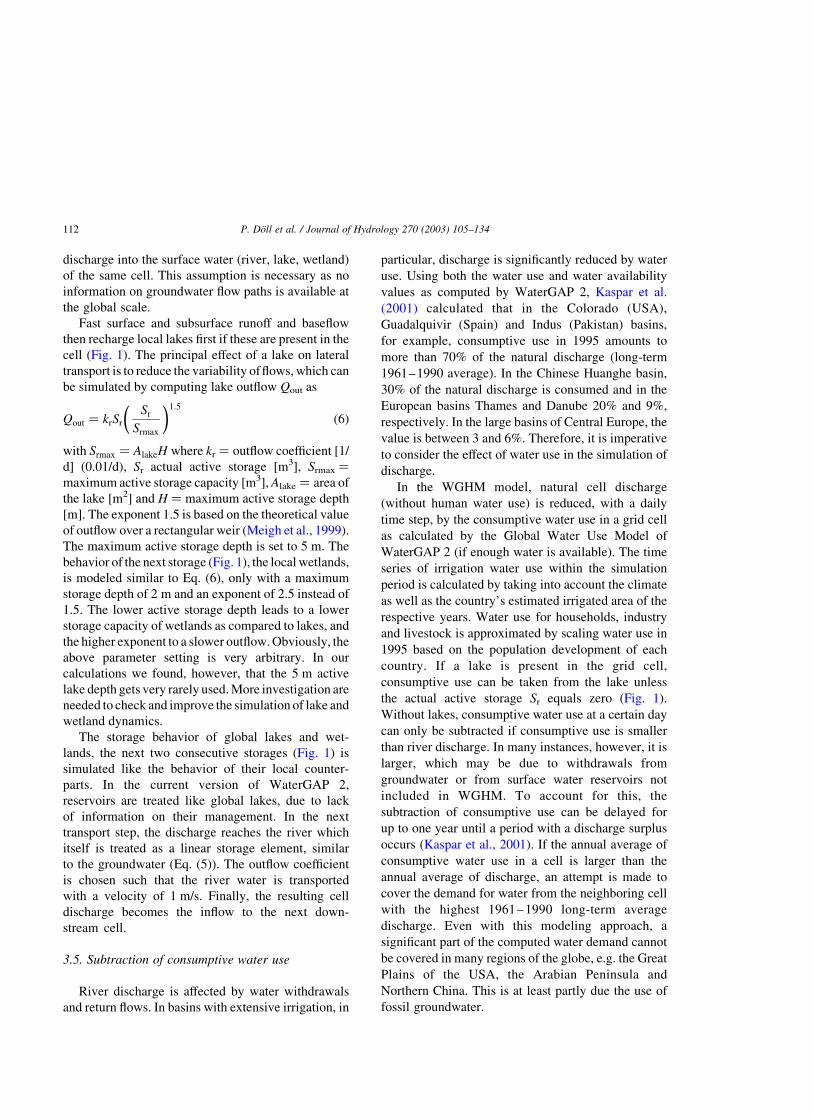
3.5. Subtraction of consumptive water use

River discharge is affected by water withdrawals

and return flows. In basins with extensive irrigation, in

particular, discharge is significantly reduced by water

use. Using both the water use and water availability

values as computed by WaterGAP 2, Kaspar et al.

(2001) calculated that in the Colorado (USA),

Guadalquivir (Spain) and Indus (Pakistan) basins,

for example, consumptive use in 1995 amounts to

more than 70% of the natural discharge (long-term

1961–1990 average). In the Chinese Huanghe basin,

30% of the natural discharge is consumed and in the

European basins Thames and Danube 20% and 9%,

respectively. In the large basins of Central Europe, the

value is between 3 and 6%. Therefore, it is imperative

to consider the effect of water use in the simulation of

discharge.

In the WGHM model, natural cell discharge

(without human water use) is reduced, with a daily

time step, by the consumptive water use in a grid cell

as calculated by the Global Water Use Model of

WaterGAP 2 (if enough water is available). The time

series of irrigation water use within the simulation

period is calculated by taking into account the climate

as well as the country’s estimated irrigated area of the

respective years. Water use for households, industry

and livestock is approximated by scaling water use in

1995 based on the population development of each

country. If a lake is present in the grid cell,

consumptive use can be taken from the lake unless

the actual active storage Sr equals zero (Fig. 1).

Without lakes, consumptive water use at a certain day

can only be subtracted if consumptive use is smaller

than river discharge. In many instances, however, it is

larger, which may be due to withdrawals from

groundwater or from surface water reservoirs not

included in WGHM. To account for this, the

subtraction of consumptive use can be delayed for

up to one year until a period with a discharge surplus

occurs (Kaspar et al., 2001). If the annual average of

consumptive water use in a cell is larger than the

annual average of discharge, an attempt is made to

cover the demand for water from the neighboring cell

with the highest 1961–1990 long-term average

discharge. Even with this modeling approach, a

significant part of the computed water demand cannot

be covered in many regions of the globe, e.g. the Great

Plains of the USA, the Arabian Peninsula and

Northern China. This is at least partly due the use of

fossil groundwater.


3.6. Model tuning

It is unlikely that a large-scale hydrological model

can simulate actual runoff and discharge satisfactorily

if it is not adjusted in a basin-specific manner based on

observed discharge. The main reasons for this are:

† erroneous input data (precipitation, in particular, as

well as radiation)

† sub-grid spatial heterogeneity

† uncertainty with respect to model algorithms (e.g.

computation of potential evapotranspiration or

discharge reduction by water use)

† neglect of important processes like surface water-

groundwater interaction (river losses, capillary

rise), the formation of small ponding after short

lateral transport and artificial transfers.

Observed discharge provides additional infor-

mation, and tuning against these measurement values

can therefore improve model performance. In order to

avoid overparameterization and to enable model

tuning in a large number of basins, only the vertical

water balance for the land area is tuned by adjusting

one model parameter, the runoff coefficient g (compare

Eq. (3)). The goal of our tuning process is to ensure that

the long-term average discharges are well represented

by the model as they typically form the basis for water

stress indicators (Alcamo et al., 2000; Raskin et al.,

1997). WGHM has been tuned for 724 drainage basins

worldwide (Fig. 2), based on observed discharges

provided by GRDC (Global Runoff Data Centre)

(1999) Koblenz, Germany, in 1999. The minimum

drainage basin size considered is 9000 km2, and the

stations along a river were selected such that the inter-

station areas are generally larger than 20,000 km2. The

model is tuned to discharge of the last thirty

measurement years (or fewer years, depending on

data availability). The tuning basins cover about 50%

of the global land area (not considering Greenland and

Antarctica) and about 70% of the actively discharging

area (Fekete et al., 1999).

In the tuning process, the runoff coefficient of all

cells within each individual basin is adjusted homo-

geneously such that the simulated long-term average

discharge at the tuning stations is within 1% of the

observed one. The runoff coefficient is allowed to vary

only in the range between 0.3 and 3. With a g below

0.3, considerable runoff will be produced even if the

soil is very dry, while with a g above 3, runoff will be

Fig. 2. Location of tuning basins and selected discharge gauging stations (tuning and validation stations referred to in Tables 3 and 4 and Figs.

10–13).


extremely small even well above the wilting point

(compare Eq. (3)). Thus, a runoff coefficient outside

the range of 0.3–3 would prevent the hydrological

model from simulating the soil water dynamics in a

realistic manner. However, even tuning of the soil

water balance within plausible limits can, under

certain circumstances, lead to an unrealistic simu-

lation of the soil dynamics as it tries to compensate for

input data errors, spatial heterogeneity and model

formulation errors (see above).

If discharge is underestimated even with a g of 0.3,

or overestimated even with a g of 3, we suspect that

processes have a strong impact which are not taken into

account by WGHM (e.g. leakage through river beds) or

that input data, in particular precipitation, are signifi-

cantly inaccurate. In these cases, a runoff correction

factor is assigned to each cell within the basin (same

value for each cell), to enforce that the simulated and

observed long-term average discharges at the basin

outlet are within 1%. This runoff correction, however,

is complicated by the fact that some of the cells in a

basin may have a negative total cell runoff. Negative

values are due to global lakes and wetlands in which

evaporation of water supplied from upstream is larger

than precipitation. If, for example, the computed

discharge is smaller than the observed one even with

a g of 0.3, total cell runoff in each cell of the basin is

increased by adding the same percentage of its absolute

value. In order to prevent a sign change of runoff, i.e.

that the runoff from land becomes negative or the

runoff from open water surface switches from negative

to positive, a maximum change of 100% is allowed. In

basins where such a runoff correction factor has to be

applied, the model does not correctly simulate the

dynamics of the water cycle but only serves to

interpolate measured discharge in space and time.

In some basins, the correction of the cell runoff

within the tuning basin still does not lead to an

agreement between observed and measured discharge.

In this case, a second correction is applied directly to

the discharge at the measurement station. This

discharge correction is done to achieve that the

simulated inflow to the downstream drainage basin is

similar to the observed values, and leads to a stepwise

increase or decrease of discharge from the cell

upstream of the measurement cell to the measurement

cell itself. The simulated runoff field is not modified by

this discharge correction.

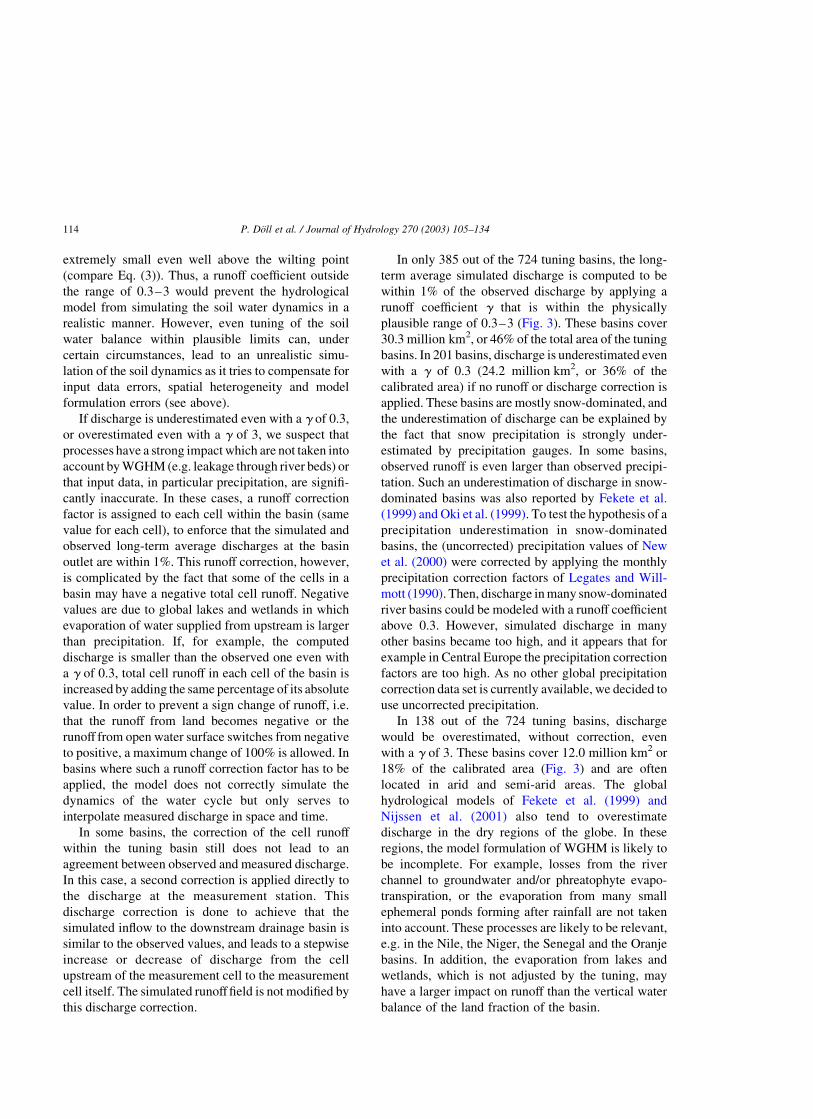
In only 385 out of the 724 tuning basins, the long-

term average simulated discharge is computed to be

within 1% of the observed discharge by applying a

runoff coefficient g that is within the physically

plausible range of 0.3–3 (Fig. 3). These basins cover

30.3 million km2, or 46% of the total area of the tuning

basins. In 201 basins, discharge is underestimated even

with a g of 0.3 (24.2 million km2, or 36% of the

calibrated area) if no runoff or discharge correction is

applied. These basins are mostly snow-dominated, and

the underestimation of discharge can be explained by

the fact that snow precipitation is strongly under-

estimated by precipitation gauges. In some basins,

observed runoff is even larger than observed precipi-

tation. Such an underestimation of discharge in snow-

dominated basins was also reported by Fekete et al.

(1999) and Oki et al. (1999). To test the hypothesis of a

precipitation underestimation in snow-dominated

basins, the (uncorrected) precipitation values of New

et al. (2000) were corrected by applying the monthly

precipitation correction factors of Legates and Will-

mott (1990). Then, discharge in many snow-dominated

river basins could be modeled with a runoff coefficient

above 0.3. However, simulated discharge in many

other basins became too high, and it appears that for

example in Central Europe the precipitation correction

factors are too high. As no other global precipitation

correction data set is currently available, we decided to

use uncorrected precipitation.

In 138 out of the 724 tuning basins, discharge

would be overestimated, without correction, even

with a g of 3. These basins cover 12.0 million km2 or

18% of the calibrated area (Fig. 3) and are often

located in arid and semi-arid areas. The global

hydrological models of Fekete et al. (1999) and

Nijssen et al. (2001) also tend to overestimate

discharge in the dry regions of the globe. In these

regions, the model formulation of WGHM is likely to

be incomplete. For example, losses from the river

channel to groundwater and/or phreatophyte evapo-

transpiration, or the evaporation from many small

ephemeral ponds forming after rainfall are not taken

into account. These processes are likely to be relevant,

e.g. in the Nile, the Niger, the Senegal and the Oranje

basins. In addition, the evaporation from lakes and

wetlands, which is not adjusted by the tuning, may

have a larger impact on runoff than the vertical water

balance of the land fraction of the basin.


Fig. 3. River basins in which WGHM can be tuned by adjusting the runoff coefficient within plausible limits (0.3–3).

P.

Doll

eta

l./

Jou

rna

lo

fH

ydro

log

y2

70

(20

03

)1

05

–1

34

11

5

In river basins with large consumptive water use, a

relatively small underestimation of subtracted con-

sumptive use might lead to an overestimation of

discharge (e.g. Murray-Darling in Australia, lower

stretches of the Danube in Romania and Bulgaria). In

addition, in some basins river flow is affected by

interbasin transfers, a process that is not simulated in

WGHM. In the case of the lower Colorado, about 30%

of the discharge is exported to adjoining water-scarce

basins (Smedena, 2000). The relatively small over-

estimation of discharge in the French rivers Seine,

Loire and Rhone is possibly related to interbasin

transfers, too.

In 103 out of the 339 tuning basins in which cell

runoff is corrected an additional discharge correction

factor had to be introduced. Discharge was corrected

downwards in 43 basins (6.4 million km2), e.g. in

basins where river discharge decreases in the down-

stream direction (e.g. Orange, Colorado). An upward

correction was needed in 60 mainly snow-dominated

basins (5.7 million km2), e.g. in many Canadian

basins as well as in the Brahmaputra and the Irrawady

basins, where observed precipitation is underesti-

mated due to the insufficiently dense precipitation

station network (Nijssen et al., 2001).

3.7. Regionalization

Runoff coefficients in the untuned river basins were

estimated using a multiple linear regression approach

that included tuning basins with the following

characteristics:

† The basin is the most upstream sub-basin of the

river basin. This ensures that its tuning has not

been influenced by the tuning in upstream basins.

† The basin area is at least 20,000 km2.

† If the runoff coefficient of the tuning basin is 0.3, the

1961–1990 long-term average annual temperature

of the basin is below 10 8C. (This includes a large

number of snow-dominated basins but excludes a

few tropical basins for which we do not see a

consistent explanation of their low g-value).

The runoff coefficients g of the selected 311 tuning

basins were found to be correlated to three basin-

specific variables (in decreasing order of predictive

capability):

1. 1961–1990 long-term average temperature Ta of

the basin,

2. area of open freshwater (with wetlands at their

maximum extent) in percent of the total basin area

Aof

3. the length of non-perennial river stretches within

each basin Lnp (derived from the Digital Chart of

the World, ESRI, 1993).

The three variables were tested to be not inter-

correlated. A corrected R 2 of 0.53 was obtained with

respect to the regression equation

ln g ¼ 20:5530 þ 0:0466Ta 2 0:0143Aof

þ 0:0817ln Lnp ð7Þ

Everything else being equal, the smaller the runoff

coefficient is, the higher the runoff becomes. Eq. (7)

reflects that the runoff coefficient is mostly small in

cold, snow-dominated basins and high in warm, dry

regions. Eq. (7) was used to compute the runoff

coefficients of the regionalized basins, but values were

constrained to the range of 0.3–3. Correction factors

were not regionalized, i.e. correction factors were set

to 1 for all regionalized basins, which may lead to an

underestimation of runoff in regionalized basins with

g ¼ 0.3 and to an overestimation in basins with g ¼ 3.

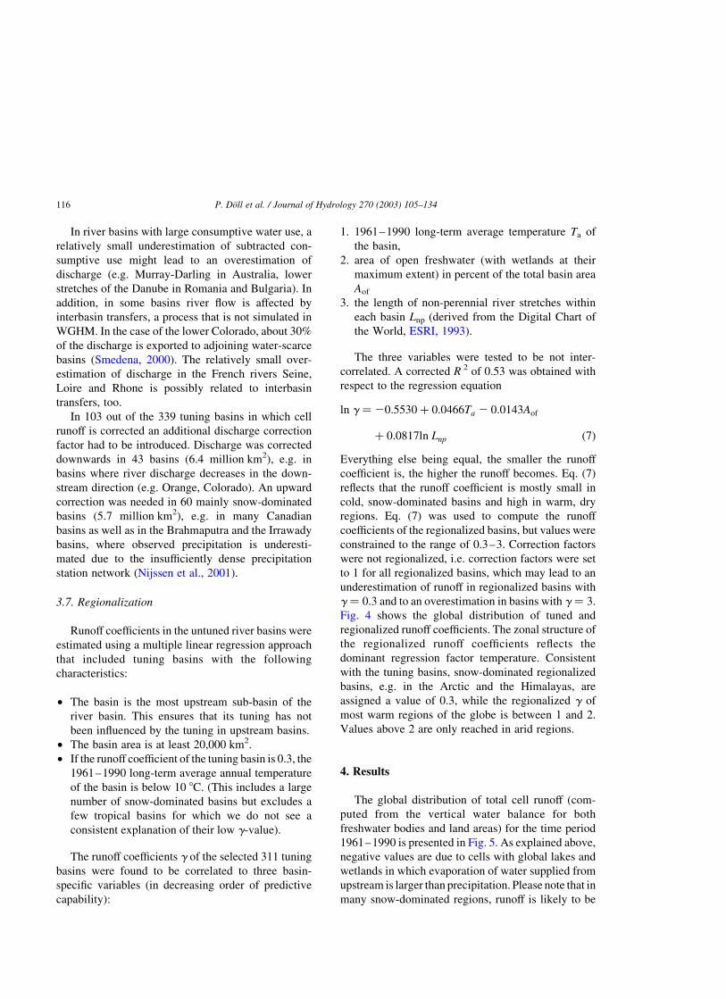
Fig. 4 shows the global distribution of tuned and

regionalized runoff coefficients. The zonal structure of

the regionalized runoff coefficients reflects the

dominant regression factor temperature. Consistent

with the tuning basins, snow-dominated regionalized

basins, e.g. in the Arctic and the Himalayas, are

assigned a value of 0.3, while the regionalized g of

most warm regions of the globe is between 1 and 2.

Values above 2 are only reached in arid regions.

4. Results

The global distribution of total cell runoff (com-

puted from the vertical water balance for both

freshwater bodies and land areas) for the time period

1961–1990 is presented in Fig. 5. As explained above,

negative values are due to cells with global lakes and

wetlands in which evaporation of water supplied from

upstream is larger than precipitation. Please note that in

many snow-dominated regions, runoff is likely to be


Fig. 4. Runoff coefficients obtained by tuning to measured discharge and by regionalization to river basins without measured discharge.

P.

Doll

eta

l./

Jou

rna

lo

fH

ydro

log

y2

70

(20

03

)1

05

–1

34

11

7

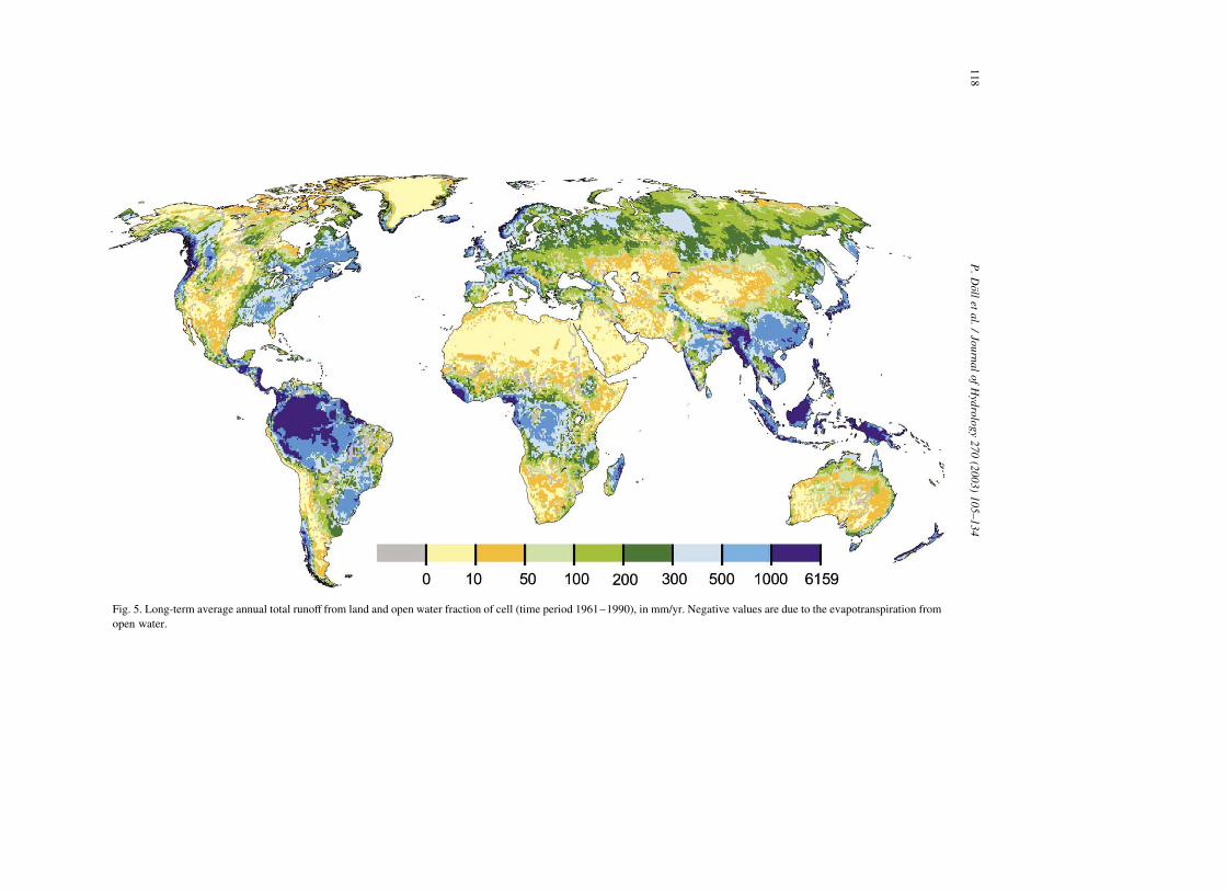
Fig. 5. Long-term average annual total runoff from land and open water fraction of cell (time period 1961–1990), in mm/yr. Negative values are due to the evapotranspiration from

open water.

P.

Doll

eta

l./

Jou

rna

lo

fH

ydro

log

y2

70

(20

03

)1

05

–1

34

11

8

underestimated, namely in those tuned areas where a

discharge correction was necessary (compare Section

3.6) as well as in those areas for which no discharge

measurements were available as the runoff correction

factor was not regionalized. For tuned semi-arid and

arid areas, WGHM possibly tends to underestimate

runoff generation as WGHM does not capture some of

the complex processes that affect the transfer of runoff

to observable river discharge (e.g. leakage from river

channels). In basins without discharge measurement,

the accuracy of the modeled runoff is unknown; in

central Australia, however, the model obviously over-

estimates runoff.

By accumulating the discharges into the oceans

and to inner-continental sinks (e.g. Lake Chad),

continental and global water resources are esti-

mated, and can be compared to previous estimates

(Table 1). For the computation of continental water

resources we use the natural discharge as if no

discharge reduction would occur due to human

water use. According to the Global Water Use

Model of WaterGAP 2, global consumptive water

use was 1250 km3/yr in 1995 (assuming 1961–

1990 long-term average climate for the compu-

tation of irrigation water use). Therefore, our

estimates should be above those of the other

authors who directly used observed discharge to

obtain their runoff estimates, without taking into

account discharge reduction by water use. How-

ever, WGHM results in the second lowest value of

global water resources. In the case of Europe, Asia,

and North and Central America, our estimates

might actually be somewhat too low as in these

areas precipitation is likely to be underestimated,

and the effect of this underestimation on discharge

is only compensated in the tuned basins (Fig. 2). In

general, the differences between the six indepen-

dent estimates of global long-term average water

resources, which encompass a range between

36,000 and 44,000 km3/yr, are much higher than

the global consumptive water use.

While long-term averages of runoff and discharge

are indicative of the spatially heterogeneous distri-

bution of water resources, they cannot be regarded as

exhaustive indicators for water availability. Interann-

ual and seasonal variability needs to be taken into

account to assess water stress that arises from a

discrepancy between water demand and water avail-

ability. To show the impact of interannual variability

on water availability, the runoff in the cell-specific 1-

in-10 dry year is compared to the long-term average

total cell runoff of the time period 1961–1990 (in 90%

Table 1

Comparison of estimated long-term average continental discharge into oceans and inland sinks, in km3/yr

Continent WaterGAP 2a Nijssen et al.(2001,Table 4)b

WRI(WorldResourcesInstitute)(2000)c

Fekete et al.(1999,Table 4)c

Korzun et al.(1978,Table 157)c

Baumgartnerand Reichel(1975, Table 12)c

Europed 2763 936 n.a. n.a. 2673 2970 2800Asiad 11234 2052 n.a. n.a. n.a. 14100 12200Africa 3529 1200 3615 4040 4474 4600 3400North and Central Americae 5540 1980 6223 7770 6478 8180 5900South America 11382 4668 10180 12030 11708 12200 11100Oceaniaf 2239 924 1712 2400 n.a. 2510 2400Total land area(except Antarctica)

36687 11760 36006 42650 39476 44290 37700

In the case of the WaterGAP 2 estimates, the values in italics are an estimate of long-term average water availability based on the 90%

reliable monthly discharge Q90. n.a.: estimate not available for chosen definition of continental extent.a Average 1961–1990.b Average 1980–1993, computed by multiplying runoff with continental areas of WaterGAP 2.c Time period not specifiedd Eurasia is subdivided into Europe and Asia along the Ural; Turkey is assigned to Asia.e Includes Greenlandf Includes the whole island of New Guinea


Fig. 6. Relative reduction of total runoff in 1-in-10 dry year as compared to the long-term average annual total runoff (time period 1961–1990), in %.

P.

Doll

eta

l./

Jou

rna

lo

fH

ydro

log

y2

70

(20

03

)1

05

–1

34

12

0

of the years, runoff is higher than in the 1-in-10 dry

year). Fig. 6, together with Fig. 5, shows that

interannual runoff variability is highest in those

regions of the globe with a low average cell runoff.

The 1-in-10 dry year runoff provides a stronger spatial

discrimination of the water resources situation than the

long-term average runoff and represents the situation

in a potential crisis year; therefore, it is a useful

additional indicator of water availability.

Whenever annual averages are considered in an

assessment of water availability, it is implicitly

assumed that storage capacities (e.g. in aquifers or

man-made reservoirs) exist to make the total annual

discharge available whenever it is needed. How-

ever, this is only the case in a few strongly

developed drainage basins like the Egyptian Nile.

In the other basins, the discharge during the

periods of high flow can generally not be used to

fulfill human water demand. Therefore, a water

availability indicator which takes into account

seasonal variability is needed. The 90% reliable

monthly discharge Q90, which is equal to the

discharge that is exceeded in 9 out of 10 months,

provides an estimate of the discharge that can be

relied on for water supply. The Q90 derived from

WGHM calculations takes into account any

reduction of natural discharge by upstream con-

sumptive water use. The global distribution of the

1961–1990 Q90 (Fig. 7) shows that discharge and

thus water availability is concentrated along the

major river courses, in particular in arid and semi-

arid zones. The spatial heterogeneity of Q90 is

higher than that of the long-term average dis-

charges (not shown). A continental aggregation of

the Q90 discharged into the oceans and inner-

continental sinks is also provided in Table 1. It

represents the annual renewable discharge that is

available if it is assumed that the amount of water

that can be used in each month of the year is

equal to the Q90-value. At the global scale, the thus

computed water availability is only 32% of the

long-term average water resources. The continent

which shows the highest seasonal variability of

discharges is Asia, where only 18% of long-term

annual water resources is reliably available. South

America is the continent with the lowest seasonal

variability, and the Q90 water availability accounts

for 41% of the total water resources.

5. Model performance

In this section, we discuss the ability of WGHM to

compute the water availability indicators presented

above. In Sections 5.1 and 5.2, the performance of

WGHM at the tuning stations is shown, and in Section

5.3. the performance in other cells (validation

stations).

5.1. Global analysis of tuning stations

WGHM is tuned such that the simulated long-term

average discharge is within 1% of the observed value.

However, the temporal dynamics of the model, i.e. the

year-to-year or month-to-month variability of dis-

charge, are not directly affected by the tuning process.

Therefore, the comparison of simulated and observed

annual and monthly discharge time series at the tuning

stations can serve to test the model performance. The

quality of simulating the interannual variability of

discharge at the tuning points is measured by the

modeling efficiency (Janssen and Heuberger, 1995)

with respect to annual discharge values AME. The

modeling efficiency, also known as Nash–Sutcliffe

coefficient, relates the goodness-of-fit of the model to

the variance of the measurement data and thus

describes the modeling success with respect to the

mean of the observations. Different from the corre-

lation coefficient, it indicates a high model quality only

if the long-term average discharge is captured well. If

AME is larger than 0.5, the interannual variability of

discharge is represented well by the computation.

Fig. 8 presents the AME of all 724 tuning basins

and shows the capability of WGHM to simulate the

sequence of wet and dry years. AME indicates how

well runoff or discharge in the 1-in-10 dry year can be

modeled. In most of Europe and the USA, AME is

above 0.5, and for many basins, AME is even above

0.7. All the basins in China and most of the Siberian

basins show an AME higher than 0.5, while the

situation in mixed in the rest of Asia. The Ganges, the

lower Indus, the Amu Darya and some smaller basins

in Central India are modeled well with respect to their

interannual variability, but other basins including the

Brahmaputra, Irrawaddy, Syr Darya and most basins

in the Near East are not. In the case of the

Brahmaputra and Irrawady, this might be related to

an inaccurate precipitation input (compare Section


Fig. 7. 90% reliable monthly discharge Q90 (time period 1961–1990), in km3/month.

P.

Doll

eta

l./

Jou

rna

lo

fH

ydro

log

y2

70

(20

03

)1

05

–1

34

12

2

Fig. 8. Modeling efficiency of annual discharges at 724 tuning stations (for the respective tuning periods).

P.

Doll

eta

l./

Jou

rna

lo

fH

ydro

log

y2

70

(20

03

)1

05

–1

34

12

3

3.6). In Africa, most basins north of the equator do not

perform well, while the interannual variability of the

Central African Congo and the semi-arid to arid

Southern African basins of the Zambezi and Orange is

captured. Model performance on the American

continent outside the USA is variable, and for most

of the Australian basins it is satisfactory. In general,

the likelihood of a good AME is higher for basins that

do not require runoff correction (compare Fig. 3).

However, even some of the other basins reach good

AME, e.g. the lower Danube (Europe), the Yangtze

(China), the Murray–Darling (Australia) and the

Orange (South Africa) basins. Table 2 shows that

snow-dominated basins (with more than 30% of the

long-term average precipitation falling as snow)

perform worse than the other basins. In the case of

humid and semi-arid/arid basins that are not snow-

dominated, 54 and 53%, respectively, of all tuning

basins have an AME greater than 0.5, and 34% of the

humid basins and 27% of the semi-arid/arid one have

an AME that is even above 0.7, compared to only 13%

of the snow-dominated basins

The modeling efficiency with respect to monthly

discharge values MME takes into account the coinci-

dence of simulated and observed discharge in each

individual month. A rather small temporal lag between

measured and observed peaks will lead to a negative

MME (compare Section 5.2 below). For most tuning

basins, MME is below 0.5; exceptions are, for

example, the Ganges and Yangtze basins and basins

in Siberia and Western Europe.

The capability of WGHM to simulate the 90%

reliable monthly discharge Q90 is checked by

comparing simulated Q90-values to those derived

from the time series of observed discharges.

Unfortunately, the observed discharge time series

are often too short to derive a reliable value of

observed Q90. For the comparison, only those 380

stations were selected which have been tuned for at

least 15 complete measurement years and represent a

drainage area of more than 20,000 km2. Fig. 9 (left)

shows the correspondence between simulated and

observed Q90. Obviously, the very high modeling

efficiency of 0.98 is due to the good fit of the two

largest values. For some basins, in particular the

smaller ones, simulated and observed Q90 differ by a

factor of 10, but for most basins, the difference is

less than a factor of 2. While this check illustrates

the capability of the model to derive realistic

estimates of Q90 (in km3/month), the quality of

Table 2

Global summary of WGHM model performance with respect to the modeling efficiency of the annual river discharges AME and the 90%

reliable monthly discharge Q90, distinguishing three classes of tuning basins: humid basins, semi-arid and arid basins, and snow-dominated

basins

Humida Semi-arid and aridb Snow-dominatedc Total

AME

Total number of tuning basins 389 191 144 724

% of basins with AME . 0.7 34 27 13 28

% of basins with 0.5 , AME # 0.7 20 26 31 24

Q90

Total number of tuning basins considered for Q90 comparisond 201 91 88 380

% of basins where difference between observed and simulated Q90

is smaller than 10% of the long-term average discharge

48 74 40 53

% of basins where difference between observed and simulated Q90

is 10–20% of the long-term average discharge

31 16 26 26

Average absolute difference between observed and simulated Q90 in

% of long-term average discharge

12 10 17 13

a Basins in which long-term average (1961–1990) precipitation is more than 50% of long-term average potential evapotranspiration (but not

snow-dominated)b Basins in which long-term average (1961–1990) precipitation is less or equal 50% of long-term average potential evapotranspiration (but

not snow-dominated)c Basins where more than 30% of the precipitation falls as snowd Basins with drainage areas greater han 20,000 km2, and observed discharge series of at least 15 years


the model with respect to the translation of

precipitation into discharge is better judged by

comparing the Q90 per unit drainage basin area (in

mm/month). The area-specific Q90 filters out the

impact of the drainage basin size. Modeling

efficiency for the area-specific Q90 is reduced to

0.67 (Fig. 9 right). If only the 144 stations with

discharge observations for the whole period of

1961–1990 are considered (hence the observed

area-specific Q90 is more reliable), model efficiency

increases to 0.73. Finally, it increases to 0.81 if from

the previous selection only the 97 basins with an

area of more than 50,000 km2 are taken into account.

For basins smaller than 20,000 km2, the modeling

efficiency is low. We conclude that the performance

of WGHM with respect to simulating Q90 is

satisfactory for basins with at least 20,000 km2,

and improves with increasing basin size.

Table 2 provides summary statistics of the model

performance with respect to Q90. In 79% of the 380

basins, the difference between simulated and observed

Q90 is less than 20% of the long-term average

discharge, and in 53%, it is even less than 10%. In

semi-arid/arid basins, the average difference between

simulated and observed is 10% of the long-term

average discharge, while it is 13% and 17% in the case

of humid and snow-dominated areas, respectively.

5.2. Selected tuning stations

To get a better impression of the quality of

WGHM, its performance at eight selected stations

with long time series of observed discharge is

discussed in the following. Fig. 2 shows the location

of these stations, and Table 3 lists observed and

simulated discharge variables, long-term average

discharge, 90% reliable monthly discharge Q90 and

10% reliable monthly discharge Q10. Besides, it

provides the modeling efficiencies for monthly

(MME) and annual (AME) discharges as well as the

basin area and the area-specific discharge. As an

example, Fig. 10 shows the time series of annual (top)

and monthly (bottom) discharges of the Polish Wisla

river (at gauging station Tczew). With an AME of

0.65, the sequence of observed wet and dry years is

captured well by the model, even though there is a

slight overestimation of observed discharge in the

1960s and an underestimation in particular in 1980.

The monthly time series has a MME of 0.54. The

underestimation in the summer months is particularly

high in the 1960s, while the high peak flows in the

summer of 1980 are clearly missed by the model. In

general, low flows of the Wisla are represented very

well by WGHM, which is shown by the very good

correspondence of simulated and observed Q90

(Table 3). The high flows as expressed by the monthly

Q10 are somewhat lower than in reality. This can also

be seen in Fig. 11, which shows the mean monthly

hydrograph of the period 1961–1990. The under-

estimation of flow in January and February and the

overestimation in March and April is rather typical for

WGHM in the case of river basins with seasonal

snow. This is due to the simple snow modeling

Fig. 9. Comparison of simulated and observed 90% monthly reliable discharge Q90 for the 380 tuning stations with a drainage area of more than

20,000 km2 and an observed time series of at least 15 years (for the respective tuning periods). Left: Q90 in km3/month, right: area-specific Q90

in mm/month.


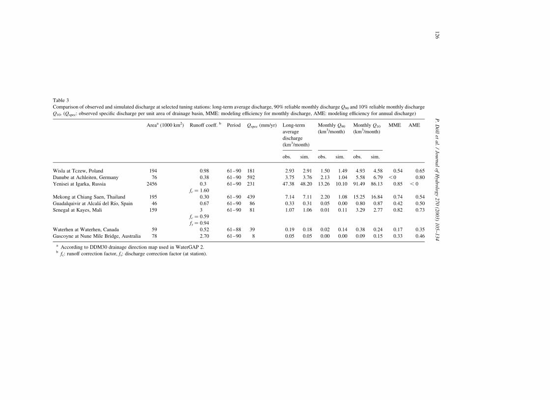
Table 3

Comparison of observed and simulated discharge at selected tuning stations: long-term average discharge, 90% reliable monthly discharge Q90 and 10% reliable monthly discharge

Q10. (Qspec: observed specific discharge per unit area of drainage basin, MME: modeling efficiency for monthly discharge, AME: modeling efficiency for annual discharge)

Areaa (1000 km2) Runoff coeff. b Period Qspec (mm/yr) Long-term

average

discharge

(km3/month)

Monthly Q90

(km3/month)

Monthly Q10

(km3/month)

MME AME

obs. sim. obs. sim. obs. sim.

Wisla at Tczew, Poland 194 0.98 61–90 181 2.93 2.91 1.50 1.49 4.93 4.58 0.54 0.65

Danube at Achleiten, Germany 76 0.38 61–90 592 3.75 3.76 2.13 1.04 5.58 6.79 ,0 0.80

Yenisei at Igarka, Russia 2456 0.3 61–90 231 47.38 48.20 13.26 10.10 91.49 86.13 0.85 , 0

fc ¼ 1.60

Mekong at Chiang Saen, Thailand 195 0.30 61–90 439 7.14 7.11 2.20 1.08 15.25 16.84 0.74 0.54

Guadalquivir at Alcala del Rıo, Spain 46 0.67 61–90 86 0.33 0.31 0.05 0.00 0.80 0.87 0.42 0.50

Senegal at Kayes, Mali 159 3 61–90 81 1.07 1.06 0.01 0.11 3.29 2.77 0.82 0.73

fc ¼ 0.59

fs ¼ 0.94

Waterhen at Waterhen, Canada 59 0.52 61–88 39 0.19 0.18 0.02 0.14 0.38 0.24 0.17 0.35

Gascoyne at Nune Mile Bridge, Australia 78 2.70 61–90 8 0.05 0.05 0.00 0.00 0.09 0.15 0.33 0.46

a According to DDM30 drainage direction map used in WaterGAP 2.b fc: runoff correction factor, fs: discharge correction factor (at station).

P.

Doll

eta

l./

Jou

rna

lo

fH

ydro

log

y2

70

(20

03

)1

05

–1

34

12

6

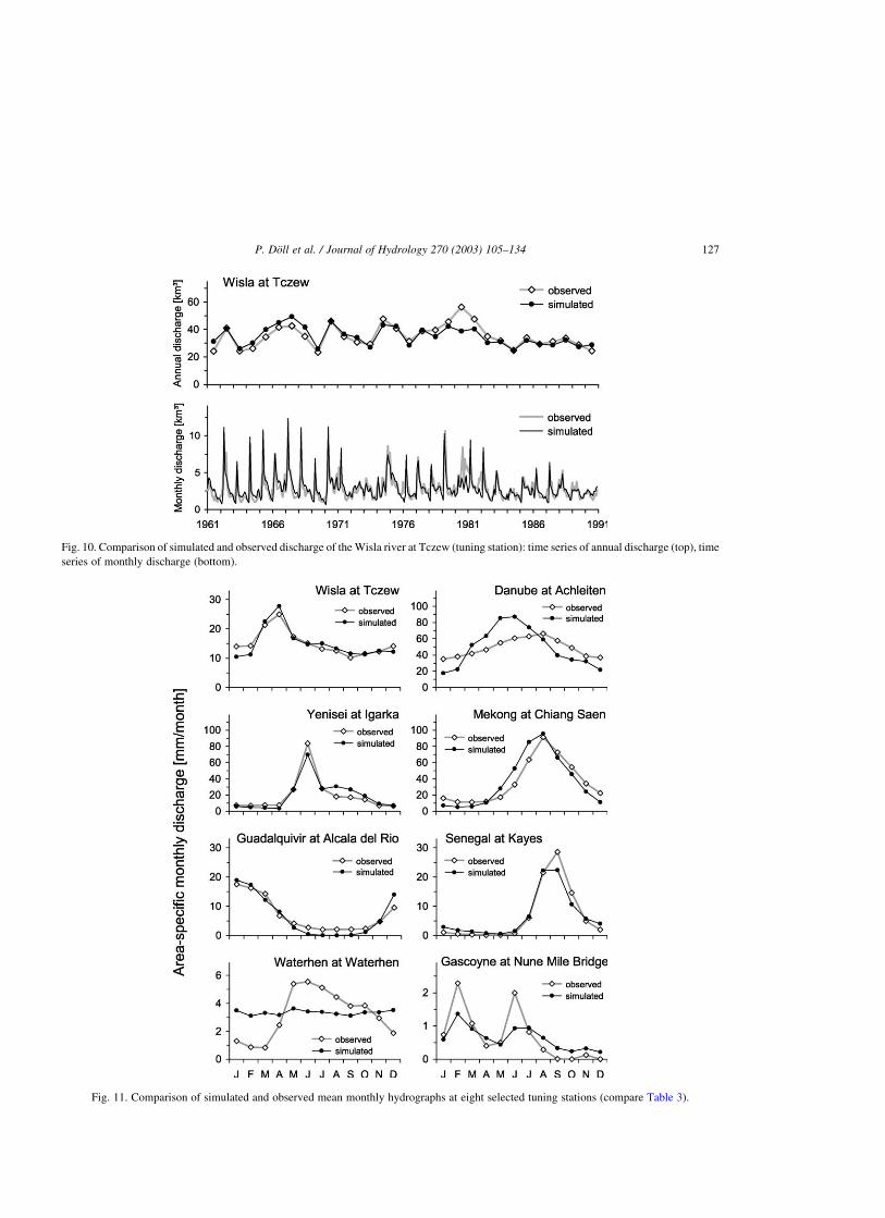
Fig. 10. Comparison of simulated and observed discharge of the Wisla river at Tczew (tuning station): time series of annual discharge (top), time

series of monthly discharge (bottom).

Fig. 11. Comparison of simulated and observed mean monthly hydrographs at eight selected tuning stations (compare Table 3).


approach of WGHM, with interpolated monthly

temperatures and a homogeneous temperature

throughout each grid cell. In the model, too much

precipitation is stored as snow until the end of the

winter, which leads to an underestimation of dis-

charge during winter and an overestimation during

spring. In reality, even in months with an average

temperature below 0 8C there are days or at least hours

above 0 8C, and due to the different microclimates

within a grid cell, not everywhere in the cell average

temperature is below 0 8C. Hence, snowfall and

snowmelt occur in a spatially and temporally more

heterogeneous way than simulated by WGHM.

The mean monthly hydrograph of the Danube at

Achleiten (Fig. 11) shows another example for the

effect of the coarse treatment of snow in the model.

Additionally, the observed peak discharge in Septem-

ber is strongly influenced by Alpine tributaries with

glacier melting (not captured in WGHM), and the

reduced seasonal variability of the observed discharge

is caused by the management of reservoirs in the

tributaries of the Danube (unknown in WGHM).

Although the seasonal behavior is not simulated

satisfactorily, the interannual variability is rep-

resented well (AME ¼ 0.80). The Yenisei at Igarka,

which requires a runoff correction probably due to the

precipitation measurement bias, is an example for the

opposite behavior. The seasonal regime being cap-

tured very well even though the basin is snow-

dominated and permafrost and freezing of the soil is

not considered in the model. The interannual

variability, however, is not correctly simulated. The

Mekong at Chiang Saen is also influenced by snow,

and at least part of the overestimated seasonal

variability of flows might by due to the coarse snow

modeling.

While the above basins are in humid regions and

have area-specific discharges between 180 and

600 mm/yr (Table 3), the next four basins shown in

Fig. 11 are in semi-arid and arid regions and have

area-specific discharges between 8 and 86 mm/yr. For

both the Guadalquivir and the Senegal, the seasonal

regime and the interannual variability are captured

quite well, even though in the (highly developed)

Guadalquivir basin, the simulated discharge drops to

zero in the summer, which is not the case in reality.

For the Senegal at Kayes, both the runoff of the basin

and the discharge at the station had to be corrected,

and the good correspondence of simulated and

observed discharge indicates that the channel and

other evaporation losses that are not simulated

explicitly by the model are proportional to the

discharge. The gauging station at the Waterhen in

Canada is located between two lakes, and the

simulation of lake storage leads to a discharge that

is almost constant throughout the year, while the

observed discharge shows a rather high seasonality.

This indicates that the simulation of lake storage in

WGHM is not adequate. The very low discharges of

the Western Australian river Gascoyne are not

represented well even though the long-term average

discharge can be modeled without any runoff or

discharge correction.

5.3. Selected validation stations

An important test of the quality of the WGHM is to

check how well simulated discharge fits to observed

discharge at gauging stations that were not used for

tuning. Like Table 3 for selected tuning stations,

Table 4 lists observed and simulated discharge

variables as well as modeling efficiencies for nine

validation stations (located in Fig. 2). Six of these

stations are located within drainage basins that were

tuned, none of them being downstream of a tuning

station. The other three are outside tuning basins, and

their runoff coefficients have been determined by

regionalization.

The most important discharge variable to be

compared is the long-term average discharge. For

the example of the Saale at Calbe, which is located

within the tuned Elbe basin (132,510 km2 at the

tuning station Neu-Darchau), the simulated long-term

average discharge is only 6% higher than the observed

value. Fig. 12 shows the time series of annual (top)

and monthly (bottom) discharges of the Saale at

Calbe. The interannual variability is captured quite

well (AME ¼ 0.65), while the monthly discharges

show a rather low correspondence (MME ¼ 0.31).

Before 1988, the WGHM often simulates a very low

discharge in January, probably due to freezing

conditions. After 1991, the summer low flows were

not captured well anymore, which might be due to

neglecting capillary rise from the groundwater, a

process which possibly became important due to

decreased drainage of lowlands after the reunification


Table 4

Comparison of observed and simulated discharge at selected gauging stations that have not been used for model tuning (validation stations): long-term average discharge, 90%

reliable monthly discharge Q90 and 10% reliable monthly discharge Q10

p Areaa (1000 km2) Runoff coeff.b Period Qspec (mm/yr) Long-term

average

discharge

(km3/month)

Monthly Q90

(km3/month)

Monthly Q10

(km3/month)

MME AME

obs. Sim. obs. sim. obs. sim.

Saale at Calbe, Germany 23 0.76 c 81–95 167 0.32 0.34 0.16 0.17 0.53 0.55 0.31 0.65

Maas at Borgharen, Belgium 22 3 c 61–90 338 0.62 0.70 0.09 0.15 1.47 1.49 0.75 0.82

fc ¼ 0.90

Mamore at Guajara–Mirim, Brazilc 614 0.59 c 71–90 438 22.39 22.51 5.23 6.11 41.48 45.02 ,0 ,0

22.44 8.31 41.10 0.78 0.40

Ica at Ipiranga Velho, Brazil 108 0.3 c 80–90 2098 18.88 18.11 11.41 13.29 26.30 23.66 0.17 ,0

fc ¼ 1.28

Zambezi at Katima Mulilo, Namibiad 329 2.26 c 65–89 126 3.46 2.21 0.84 0.09 8.39 6.74 0.15 ,0

1.60 3.25 0.24 8.39 0.80 0.74

Cimarron at Perkins, OK, USA 45 2.76 c 61–87 27 0.10 0.12 0.01 0.02 0.24 0.29 0.35 0.40

Cunene at Ruacana, Namibia 89 1.60 r 62–78 61 0.45 0.74 0.08 0.10 1.02 1.90 ,0 ,0

Okavango at Rundu, Namibia 54 2.14 r 61–89 107 0.48 0.54 0.11 0.10 1.13 1.03 0.31 ,0

Tombigbee at Coatopa AL, USA 44 1.19 r 61–87 513 1.88 1.97 0.27 0.60 4.99 4.33 0.83 0.90

(Qspec: observed specific discharge per unit area of drainage basin, MME: modeling efficiency for monthly discharge, AME: modeling efficiency for annual discharge). pdata

sources: Saale: Potsdam Institute for Climate Impact Research, Potsdam, Germany; Maas: GRDC, Brazilian rivers: Center for Sustainability and the Global Environment (SAGE),

University of Wisconsin—Madison; rivers in USA: HCDN Streamflow Data Set, 1874–1988 by J.R. Slack, Alan M. Lumb, and Jurate Maciunas Landwehr, USGS Water-

Resources Investigations Report 93-4076; rivers in Namibia: Department of Water Affairs, Windhoek, Namibia.a According to DDM30 drainage direction map used in WaterGAP 2.b c: Station in basin for which runoff coefficient was tuned against discharge at a downstream station, without tuning upstream; r: station within basin for which runoff coefficient

was determined by regionalization; fc: runoff correction factor.c In italics: results with a river transport velocity of 0.1 m/s instead of the standard value of 1 m/s.d In italics: results with a runoff coefficient of 1.6 and river transport velocity of 0.18 m/s.

P.

Doll

eta

l./

Jou

rna

lo

fH

ydro

log

y2

70

(20

03

)1

05

–1

34

12

9

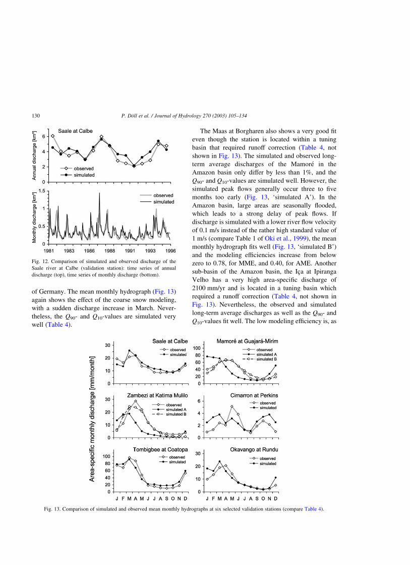
of Germany. The mean monthly hydrograph (Fig. 13)

again shows the effect of the coarse snow modeling,

with a sudden discharge increase in March. Never-

theless, the Q90- and Q10-values are simulated very

well (Table 4).

The Maas at Borgharen also shows a very good fit

even though the station is located within a tuning

basin that required runoff correction (Table 4, not

shown in Fig. 13). The simulated and observed long-

term average discharges of the Mamore in the

Amazon basin only differ by less than 1%, and the

Q90- and Q10-values are simulated well. However, the

simulated peak flows generally occur three to five

months too early (Fig. 13, ‘simulated A’). In the

Amazon basin, large areas are seasonally flooded,

which leads to a strong delay of peak flows. If

discharge is simulated with a lower river flow velocity

of 0.1 m/s instead of the rather high standard value of

1 m/s (compare Table 1 of Oki et al., 1999), the mean

monthly hydrograph fits well (Fig. 13, ‘simulated B’)

and the modeling efficiencies increase from below

zero to 0.78, for MME, and 0.40, for AME. Another

sub-basin of the Amazon basin, the Ica at Ipiranga

Velho has a very high area-specific discharge of

2100 mm/yr and is located in a tuning basin which

required a runoff correction (Table 4, not shown in

Fig. 13). Nevertheless, the observed and simulated

long-term average discharges as well as the Q90- and

Q10-values fit well. The low modeling efficiency is, as

Fig. 12. Comparison of simulated and observed discharge of the

Saale river at Calbe (validation station): time series of annual

discharge (top), time series of monthly discharge (bottom).

Fig. 13. Comparison of simulated and observed mean monthly hydrographs at six selected validation stations (compare Table 4).


in the case of the Mamore, due to overestimation of

lateral transport velocity.

The Zambezi at Katima Mulilo is within the tuning

basin of the Zambezi at Matundo Cais, with a drainage

area of more than 1.1 million km2. Discharge at

Matundo Cais is best simulated with a runoff

coefficient of 2.26, which, however, leads to a

significant discharge underestimation of 36% at

Katima Mulilo (Fig. 13, simulated A). Obviously,

the runoff generation within the large and hetero-

geneous drainage basin of the Zambezi cannot be

captured by assigning one homogeneous runoff

coefficient to the whole basin. The value of tuning

for this station is shown by adjusting both the runoff

coefficient and the lateral transport velocity. With a

runoff coefficient of 1.60 and a lateral transport

velocity of 0.18 m/s instead of 1 m/s, the long-term

average discharge is underestimated by only 6%, and

the modeling efficiencies increase to 0.80 (MME) and

0.74 (AME) (Table 4 and Fig. 13, simulated B). The

Cimarron drains a rather dry region of the Arkansas

basin. WGHM overestimates long-term average

discharge by 20% and does not represent the seasonal

regime (Fig. 13). Still, the Q90- and Q10-values are

simulated quite well.

In summary, the quality of the simulated discharge

at cells inside tuned basins appears to be reasonably

good if the basin is rather homogeneous. The

simulated long-term average discharges at the stations

inside the relatively homogeneous Central European

and Amazon basins fit well to the observed values,

which is not the case for the more heterogeneous

basins of the Zambezi and the tributaries of the

Mississippi.

Finally, the model results at three gauging stations

that are located outside of tuning basins (Fig. 2) are

checked against observations (Table 4). The long-

term average discharge in the dry Cunene basin (not

shown in Fig. 13) is overestimated by more than 60%.

This might be due to the rather low regionalized value

of the runoff coefficient of 1.60 (even though this is

the value that leads to a good fit for the nearby

Zambezi at Katima Mulilo). Long-term average

discharge in the somewhat wetter Okavango basin is

overestimated by 13%, but the simulated Q90- and

Q10-values fit the observed values well. The low flow

period is particularly well captured (Fig. 13).

However, the interannual variability is not reflected

at all by the model. The Tombigbee in the humid

Southeast of the USA is simulated very well by

WGHM (Fig. 13). The long-term average discharge is

overestimated by less than 5%, and the modeling

efficiencies are high (AME ¼ 0.90, MME ¼ 0.83).

6. Conclusions

1901–1995 time-series of 0.5 degree gridded

monthly runoff and river discharge are computed by

a tuned version of the Global Hydrological Model of

WaterGAP 2 (WGHM). Based on these time series, a

number of relevant indicators of water availability can

be computed in a consistent manner for the whole

global land area (with the exception of Antarctica).

They include 1) the long-term average annual renew-

able water resources, 2) the discharge or runoff in a

typical dry year, e.g. in the 1-in-10 dry year, and 3) the

90% reliable monthly discharge Q90. The latter two

indicators take into account the impact of interannual

and seasonal variability on water availability. On the

global average, the 90% reliable water availability is

computed to be only about one third of the long-term

average water resources.

WGHM shows the following characteristics:

† It is based on the best global data sets that are

currently available (in particular climate, drainage

directions and wetlands, lakes and reservoirs).

† Due to model tuning and, if necessary, runoff and

discharge correction, WHGM computes discharge

at more than 700 gauging stations (representing

about 50% of the global land area and 70% of the

actively discharging area) such that the simulated

long-term average discharge is within 1% of the

observed value.

† The reduction of river flow by human water

consumption is simulated based on results from

the Global Water Use Model of WaterGAP 2.

† The impact of climate variability on water

availability is taken into account. This includes

the simulation of the impact of climate variability

on upstream irrigation water requirements.

† Due to the coupling with the Global Water Use

Model, WGHM can be used to estimate the

impact of upstream water use changes on

downstream water availability.


The quality of WGHM and its capability to

simulate the above water availability indicators was

tested by comparing observed and simulated

discharge at the 724 tuning stations and also at

nine other selected gauging stations. In general, the

performance of the model with respect to comput-

ing the interannual variability as well as the 90%

monthly reliable discharge increases with increasing

basin size. We conclude that reliable results can be

obtained for basins of more than 20,000 km2.

However, basin types have been identified that

are less likely to be represented well by WGHM.

There is the tendency that semi-arid and arid basins

are modeled less satisfactorily than humid basins,

which is partially due to neglecting river channel

losses and evaporation of runoff from small

ephemeral ponds in the model. Also, the hydrology

of highly developed basins with large artificial

storages, basin transfers and irrigation schemes

cannot be simulated well. In all basins where

discharge is controlled by man-made reservoirs, its

seasonality is likely to be misrepresented by

WGHM as no information on reservoir manage-

ment is taken into account. Snow-dominated river

basins generally suffer from the underestimation of

actual precipitation. Hence, in snow-dominated

basins without a tuning station, discharge is likely

to be underestimated. The seasonality of discharge

in snow-dominated basins is not represented well

by WGHM due to the simple snow-modeling

algorithm used. River basins which are character-

ized by extensive wetlands and lakes are also

difficult to model. Even though the explicit

modeling of wetlands and lakes leads to a much

improved modeling of both the vertical water

balance and the lateral transport of water, not

enough information is included in WGHM to

accurately capture the hydrology of these water

bodies.

We conclude that model tuning which aimed at

achieving a good representation of the long-term

average discharges has a strong positive effect on

the performance of all proposed water availability

indicators. Certainly, the reliability of model results

is highest at the locations at which WGHM was

tuned. It can be assumed that also the reliability for

cells inside tuned basins is reasonably high if

the basin is relatively homogeneous. This assump-

tion is supported by the comparison of observed

and simulated discharge at the gauging stations that

were not used for tuning. No conclusion can be

drawn with respect to the reliability of model

results outside tuned basins but the discharge

analysis at the few available stations indicates an

acceptable reliability, in particular in humid

regions.

Future model improvements will focus on a

more realistic snow modeling, a refined modeling

of groundwater recharge and the simulation of river

channel losses. Besides, it is planned to include

river velocity as an additional tuning parameter.

It has been shown that WGHM is able to

compute reliable and meaningful indicators of

water availability at a high spatial resolution.

Therefore, the modeling results of WGHM are

well suited to be used in global assessments of

water security, food security and freshwater

ecosystems.

Acknowledgements

The authors thank B. Fekete and an anonymous

reviewer for their detailed and constructive

comments.

References

Alcamo, J., Leemans, R., Kreileman, E. (Eds.), 1998. Global

Change Scenarios of the 21st Century. Results of the IMAGE

2.1 Model, Pergamon, Oxford.

Alcamo, J., Henrichs, T., Rosch, T., 2000. World Water in 2025—

Global modeling and scenario analysis for the World Commis-

sion on Water for the 21st Century, Kassel World Water Series

2, Center for Environmental Systems Research, University of

Kassel, Germany, http://www.usf.uni-kassel.de/usf/archiv/

dokumente.en.htm.

Arnell, N.W., 1999a. A simple water balance model for the

simulation of streamflow over a large geographic domain.

J. Hydrol. 217, 314–335.

Arnell, N.W., 1999b. Climate change and global water resources.

Global Environ. Change 9, S31–S49.

Batjes, N.H., 1996. Development of a world data set of soil water

retention properties using pedotransfer rules. Geoderma 71,

31–52.


http://www.usf.uni-kassel.de/usf/archiv/dokumente.en.htm


Baumgartner, A., Reichel, E., 1975. The World Water Balance,

Elsevier, Amsterdam.

Bergstrom, S., 1995. The HBV model. In: Singh, V.P., (Ed.),

Computer Models of Watershed Hydrology, Water Resources

Publications, pp. 443–476.

Birkett, C.M., Mason, I.M., 1995. A new global lakes database for a

remote sensing programme studying climatically sensitive large

lakes. J. Great Lakes Res. 21 (3), 307–318.publication available

online at http://wwwcpg.mssl.ucl.ac.uk/orgs/un/glaccd/html/

mgld.html.

Brown, J., Ferrians, O.J. Jr., Heginbottom, J.A., Melnikov, E.S.,

1998. Digital Circum-Arctic Map of Permafrost and Ground-Ice

Conditions. International Permafrost Association Data and

Information Working Group, Circumpolar Active-Layer

Permafrost System (CAPS), CD-ROM version 1.0. National

Snow and Ice Data Center, University of Colorado, Boulder,

Colorado.

Canadian Geological Survey, 1995. Generalized Geological Map of

the World and Linked Databases. Open File Report 2915d. CD-

ROM.

Deardorff, J.W., 1978. Efficient prediction of ground surface

temperature and moisture, with inclusion of a layer of

vegetation. J. Geophys. Res. 86C, 1889–1903.

Doll, P., Lehner, B., 2002. Validation of a new global 30-min

drainage direction map. J. Hydrol. 258 (1–4), 214–231.

Doll, P., Siebert, S., 2002. Global modeling of irrigation water

requirements. Water Resour. Res. 38 (4), 8.1–8.10.DOI

10.1029/2001WR000355.

Doll, P., Kaspar, F., Lehner, B., 2001. The global integrated water

model WaterGAP 2.1. In: Lehner, B., Henrichs, T., Doll, P.,

Alcamo, J. (Eds.), EuroWasser, Kassel World Water Series 5,

Center for Environmental Systems Research, University of

Kassel, Germany, http://www.usf.uni-kassel.de/usf/archiv/

dokumente.en.htm.

Doll, P., Lehner, B., Kaspar, F., 2000. Global modeling of

groundwater recharge and surface runoff. EcoRegio 8, 73–80.

Doll, P., Kaspar, F., Alcamo, J., 1999. Computation of global water

availability and water use at the scale of large drainage basins.

Mathematische Geologie 4, 111–118.

ESRI (Environmental Systems Research Institute), 1992. ArcWorld

1:3 M Continental Coverage.

ESRI (Environmental Systems Research Institute), 1993. Digital

Chart of the World 1:1 M.

FAO (Food and Agriculture Organization), 1995. Digital Soil Map

of the World and Derived Soil Properties, CD-ROM Version

3.5, FAO, Rome.

Fekete, B.M., Vorosmarty, C.J., Grabs, W., 1999. Global composite

runoff fields of observed river discharge and simulated water

balances. Report No. 22, Global Runoff Data Centre, Koblenz,

Germany.

Forsythe, W.C., Rykiel, E.J., Stahl, R.S., Wu, H., Schoolfield, R.M.,

1995. A model comparison for daylength as a function of

latitude and day of year. Ecol. Model. 80, 87–95.

Geng, S., Penning, F.W.T., Supit, I., 1986. A simple method for

generating daily rainfall data. Agric. For. Meteor. 36, 363–376.

GRDC (Global Runoff Data Centre), 1999. GRDC Station Catalog

(available online athttp://www.bafg.de/html/internat/grdc/

download.html).

Holzle, M., Haberli, W., 1999. World Glacier Inventory. World

Glacier Monitoring Service. National Snow and Ice Data

Center. University of Colorado, Boulder, Colorado.

ICOLD (International Commission on Large Dams), 1998. Word

Register of Dams (CD-ROM), Paris, France.

Janssen, P.H.M., Heuberger, P.S.C., 1995. Calibration of process-

oriented models. Ecol. Model. 83, 55–66.

Kaspar, F., Doll, P., Lehner, B., 2001. Globale Modellierung der

Durchflussverminderung durch konsumptive Wassernutzung. In:

Sutmoller, J., Raschke, E. (Eds.), Modellierung in meso-bis

makroskaligen Flußeinzugsgebieten-Tagungsband zum gleich-

namigen Workshop am 16./17. November 2000 in Lauenburg,

GKSS 2001/15, GKSS Geesthacht,.

Klepper, O., van Drecht, G., 1998. WARibaS, Water Assessment on a

River Basin Scale; A computer program for calculating water

demand and satisfaction on a catchment basin level for global-

scale analysis of water stress. Report 402001009. RIVM, The

Netherlands.

Korzun, V.I., Sokolow, A.A., Budyko, M.I., Voskresensky, K.P.,

Kalininin, G.P., Konoplyanstev, A.A., Korotkevich, E.S.,

Kuzin, P.S., Lvovich, M.I. (Eds.), 1978. World Water Balance

and Water Resources of the Earth. UNESCO, Paris,.

Legates, D.R., Willmott, C.J., 1990. Mean seasonal and spatial

variability in gauge-corrected, global precipitation. Int.

J. Climatotol. 10, 111–117.

Lehner, B., Doll, P., 2001. A global lakes, reservoirs and wetlands

data set. Data set description sheet, Center for Environmental

Systems Research, University of Kassel, Germany.

Liang, X., Lettenmaier, D.P., Wood, E.F., Burges, S.J., 1994. A

simple hydrologically based model of land surface water and

energy fluxes for general circulation models. J. Geophys. Res.

D3 (99), 14415–14428.

Meigh, J.R., McKenzie, A.A., Sene, K.J., 1999. A grid-based

approach to water scarcity estimates for Eastern and Southern

Africa. Water Resour. Mgmt 13 (2), 85–115.

New, M., Hulme, M., Jones, P.D., 2000. Representing twentieth

century space-time climate variability Part II: Development of

1901-96 monthly grids of terrestrial surface climate. J. Climate

13, 2217–2238.

Nijssen, B., O’Donnell, G.M., Lettenmaier, D.P., Lohmann, D.,

Wood, E.F., 2001. Predicting the discharge of global rivers.

J. Climate 14, 3307–3323.

Oki, T., Nishimura, T., Dirmeyer, P., 1999. Assessment of annual

runoff from land surface models using Total Runoff Integrating

Pathways (TRIP). J. Meteorol. Soc. Jpn 77, 235–255.

Priestley, C., Taylor, R., 1972. On the assessment of surface heat

flux and evaporation using large scale parameters. Mon.

Weather Rev. 100, 81–92.

Raskin, P., Gleick, P., Kirshen, P., Pontius, G., Strzepek, K., 1997.

Water futures: Assessment of long-range patterns and problems.

Background paper Comprehensive Assessment of the Fresh-

water Resources of the World, Stockholm Environment

Institute, Stockholm, Sweden.


http://wwwcpg.mssl.ucl.ac.uk/orgs/un/glaccd/html/mgld.html

http://wwwcpg.mssl.ucl.ac.uk/orgs/un/glaccd/html/mgld.html



http://www.bafg.de/html/internat/grdc/download.html

http://www.bafg.de/html/internat/grdc/download.html

Shuttleworth, W.J., 1993. Evaporation. In: Maidment, D.R., (Ed.),

Handbook of Hydrology, McGraw-Hill, New York, USA, pp.

4.1–4.53.

Smedena, L., 2000. Irrigation-induced river salinization: Five major

irrigated basins in the arid zone. International Water Management

Institute, Colombo, Sri Lanka.

Vorosmarty, C.J., Federer, C.A., Schloss, A., 1998. Potential

evaporation functions compared on US watersheds: implications

for global-scale water balance and terrestrial ecosystem model-

ling. J. Hydrol. 207, 147–169.

Vorosmarty, C.J., Sharma, K., Fekete, B., Copeland, A.H., Holden,

J., Marble, J., Lough, J.A., 1997. The storage and aging of

continental runoff in large reservoir systems of the world.

Ambio 26, 210–219.

WCMC (World Conservation Monitoring Centre), 1999. Wetlands

Dataset, Cambridge, UK.

WRI (World Resources Institute), 2000. World Resources 2000–

2001, Oxford University Press, New York, USA.

Yates, D.N., 1997. Approaches to continental scale runoff for

integrated assessment models. J. Hydrol. 291, 289–310.


A global hydrological model for deriving water ... · A global hydrological model for deriving...

Documents

Transcript of A global hydrological model for deriving water ... · A global hydrological model for deriving...