A Geostatistical Approach for Dynamic Life Tables.

The effect of mortality on remaining lifetime and

annuities

A. Debona, F. Martınez-Ruizb, F. Montesb

ae-mail: andeau@eio.upv.es. Centro de Gestion de la Calidad y del Cambio. UniversidadPolitecnica de Valencia. Camino de Vera s/n. 46022 Valencia. Spain

bDpt. d’Estadıstica i I. O. Universitat de Valencia. Spain

Abstract

Dynamic life tables arise as an alternative to the standard (static) life ta-

ble with the aim of incorporating the evolution of mortality over time. The

parametric model introduced by Lee and Carter in 1992 for projected mor-

tality rates in the US is one of the most outstanding and has been largely

used since then. Different versions of the model have been developed but

all of them, together with other parametric models, consider the observed

mortality rates as independent observations. This is a difficult hypothesis to

hold when looking at the graph of the residuals obtained with any of these

methods.

Methods of adjustment and prediction based on geostatistical techniques

which exploit the dependence structure existing among the residuals are an

alternative approach to classical methods. Dynamic life tables can be consid-

ered as a two-way table on a grid equally spaced in either the vertical (age)

or horizontal (year) direction, and the data can be decomposed into a deter-

ministic large-scale variation (trend) plus a stochastic small-scale variation

(residuals).

Preprint submitted to Insurance: Mathematics and Economics February 8, 2010

Our contribution consists of applying geostatistical techniques for esti-

mating the dependence structure of the mortality data and for prediction

purposes, also including the influence of the year of birth (cohort). We com-

pare the performance of this new approach with different versions of the

Lee-Carter model. Additionally, we obtain bootstrap confidence intervals for

predicted qxt resulting from applying both methodologies, and we study their

influence on the predictions of e65t and a65t.

Key words: Life Table, Geostatistics, Bootstrap Confidence Intervals

1. Introduction

In static life tables the influence of age on data graduation has been

widely addressed in papers such as Forfar et al. (1988), Renshaw (1991) and

Debon et al. (2005), using parametric models, or in Gavin et al. (1993, 1994,

1995) and Debon et al. (2006b), who propose non-parametric models. None

of these models take into account the fact that mortality progresses over the

years, as they were designed to analyse data corresponding to one year in

particular or, in the case of several years, to work with aggregated data.

The concept of a dynamic life table seeks to solve this problem by jointly

analyzing mortality data corresponding to a series of consecutive years. This

approach allows the calendar effect influence on mortality to be studied.

A sample of the models developed for graduating dynamic tables can be

found in Benjamin and Soliman (1993); Tabeau et al. (2001); Pitacco (2004);

Wong-Fupuy and Haberman (2004); Debon et al. (2006a). Most of them

adapt traditional laws to the new situation and all them share a common

hypothesis: they consider the observed measures of mortality as independent

2

across ages and over time. As Booth et al. (2002) point out, it is difficult to

hold such a hypothesis when looking at the graph of the residuals obtained

after the adjustment with any of these models.

Tools appropriate to other disciplines can be used to overcome the prob-

lem which residual dependency supposes. We have turned to Geostatistics,

which provides techniques for modelling the dependency structure among a

set of neighbouring observations. Covariance functions and variogram are the

essential tools which, together with kriging techniques, also allow predictions

to be made and associated errors to be calculated (Matheron, 1975; Journel

and Huijbregts, 1978).

Geostatistical techniques were designed for the analysis of data which

were very far from what a dynamic table represents. This distance is only

apparent as a dynamic table can actually be considered as a set of data over

a rectangular grid equally spaced both vertically, for age, and horizontally,

for year. The diagonals of this grid stand for the cohort determined by

the age and the year. On the other hand, the aim of Geostatistics is, as

already mentioned, to model the dependence structure among neighbours,

which requires defining a neighbourhood relationship as well as a distance.

They are straightforward in the case of spatial data but also possible in other

kind of data. The analysis of sudden infant death syndrome (SIDS) in North

Carolina in Cressie (1993), as well as the analysis using spatial techniques

of the 1970 US Draft Lottery (Mateu et al., 2004), support this assessment.

Moreover, as in previous studies, we will show that these methods provide

better solutions than the classical methods since they simultaneously take

into account the effect of age and time, while the others treat both effects

3

separately.

This article is structured as follows: Section 2 introduces the original

Lee-Carter model with one and two time terms and the Lee-Carter age-

period-cohort model, derived from the original one but adding a second term

for collecting the influence of cohort over mortality. This section ends with

an introduction to geostatistical methodology, including a brief description

of the median polish algorithm that will be used for estimating the determin-

istic trend of the geostatistic model proposed. Section 3 briefly presents the

bootstrapping techniques used for obtaining confidence intervals. Section 4

presents the results of the application of the seven models, three Lee-Carter

and four median polish models, to the analysis of mortality data in Spain

for the period 1980-2003. The results of the prediction of qx,2004 and qx,2005,

death probability at age x in year 2004 and 2005, obtained from the projec-

tions of the adjusted models, are also collected in this section. The last part

of Section 4 is devoted to obtaining the confidence intervals for the predic-

tion of residual life expectancy and the annuities, e65t and a65t. The results

which provide the distinct models for the period 2004-2023 are compared, the

evolution of the annuities being of particular interest for, as far as we know,

we have not found evidence of any other similar study on mortality data in

Spain. Finally, Section 5 establishes the conclusions to be drawn from the

results in the previous section.

2. Adjustment and prediction of mortality rates

We consider a set of crude mortality rates qxt, for age x ∈ [x1, xk] and

calendar year t ∈ [t1, tn], which we use to produce smoother estimates, qxt, of

4

the true but unknown mortality probabilities qxt. A crude rate at age x and

time t is typically based on the corresponding number of deaths recorded,

dxt, relative to those initially exposed to risk, Ext.

2.1. Lee-Carter models

The Lee-Carter Model, developed in Lee and Carter (1992), consists of

adjusting the following function to the measure of mortality ,

mxt = exp(ax + bxkt + ǫxt) (1)

or, equally, the function

ln(mxt) = ax + bxkt + ǫxt, (2)

applied to its logarithm transform. This is an age-period (AP) model as the

double subscript refers to the age, x, and to the year or unit of time, t. In (1)

and (2), ax and bx are age-dependent parameters and kt is a specific mortality

index for each year or unit of time. The errors ǫxt, with a zero average and

variance σ2ǫ , reflect the historical influences of each specific age that are not

captured by the model.

Various authors have proposed modifications to the Lee-Carter model.

Booth et al. (2002) and Renshaw and Haberman (2003) propose the inclusion

of a new term in (2), of the form bxkt, with the objective of improving the

fit and trying to eliminate the trend shown by the residuals with the original

model. Renshaw and Haberman (2006) propose an age-cohort model (AC)

in which the time scale t of the original model is substituted by the cohort

c = t− x. In the same article they also propose an age-period-cohort (APC)

5

which adds a new term to (2) which, different from what is suggested in

Booth et al. (2002), includes the influence of the cohort on mortality.

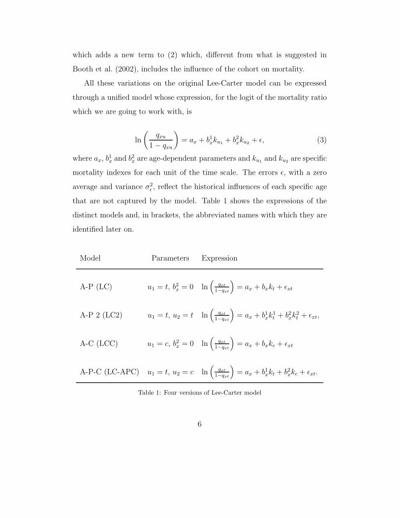
All these variations on the original Lee-Carter model can be expressed

through a unified model whose expression, for the logit of the mortality ratio

which we are going to work with, is

ln

(

qxu

1 − qxu

)

= ax + b1xku1

+ b2xku2

+ ǫ, (3)

where ax, b1x and b2

x are age-dependent parameters and ku1and ku2

are specific

mortality indexes for each unit of the time scale. The errors ǫ, with a zero

average and variance σ2ǫ , reflect the historical influences of each specific age

that are not captured by the model. Table 1 shows the expressions of the

distinct models and, in brackets, the abbreviated names with which they are

identified later on.

Model Parameters Expression

A-P (LC) u1 = t, b2x = 0 ln

(

qxt

1−qxt

)

= ax + bxkt + ǫxt

A-P 2 (LC2) u1 = t, u2 = t ln(

qxt

1−qxt

)

= ax + b1xk

1t + b2

xk2t + ǫxt,

A-C (LCC) u1 = c, b2x = 0 ln

(

qxt

1−qxt

)

= ax + bxkc + ǫxt

A-P-C (LC-APC) u1 = t, u2 = c ln(

qxt

1−qxt

)

= ax + b1xkt + b2

xkc + ǫxt.

Table 1: Four versions of Lee-Carter model

6

All these models, except the LCC, will be used to adjust the Spanish

mortality data described later on. The adjustment is carried out through

ML using the gnm library (Turner and Firth, 2006) of the R Development

Core Team (2005). In the Appendix details are added regarding the necessary

normalisation of parameters and, in particular, how to overcome the problem

which appears in the LC-APC model due to the relationship which exits

between age, period and the cohort, c = t − x.

2.2. Geostatistical methods

The mortality data we want to analyze can be considered as a set of

spatio-temporal data, with age as the unidimensional spatial component and

year as the temporal one.

Following Cressie and Majure (1997), we denote by Z(x, t) the mortality

measure at age x and time t. We suppose that we have observed the data

{Z(x, t), x ∈ D, t ∈ T}, and we wish to predict the process value Z(x0, t0) at

the age x0 ∈ D for the year t0. In order to achieve the convenient stationarity,

we assume that the data can be decomposed into a deterministic large-scale

variation (trend) plus a stochastic small-scale variation (error). The model

can be written as,

Z(x, t) = µ(x, t) + δ(x, t) (4)

where E[Z(x, t)] = µ(x, t) and δ(·, ·) is a zero-mean second order stationary

Gaussian process with covariance function

C(h, u) = Cov[Z(x + h, t + u), Z(x, t)]

and variogram

2γ(h, u) = V ar[Z(x + h, t + u) − Z(x, t)] = V ar[δ(x + h, t + u) − δ(x, t)],

7

both characterizing the spatial and temporal dependence. In fact, under

the hypothesis of second order stationarity, the variogram and covariance

function are related throughout

2γ(h, u) = 2C(0, 0) − 2C(h, u). (5)

The large-scale variation µ(x, t) and the small-scale variation δ(·, ·) are mod-

elled respectively as deterministic and stochastic processes, but there is no

way of making the decomposition identifiable.

The error process δ(x, t) can be estimated by subtracting the estimation

of µ(x, t) from (4) µ(x, t),

δ(x, t) = Z(x, t) − µ(x, t). (6)

The estimation of the covariance function can be obtained using the classical

estimator based on the moments method (Cressie (1993), Sec.2.4),

C(h, u) =1

|N(h, u)|

∑

|N(h,u)|

(

δ(xi, ti) − mδ

)(

δ(xj , tj) − mδ

)

(7)

where,

N(h, u) = {((xi, ti), (xj , tj)), xi − xj = h, ti − tj = u} (8)

|N(h, u)| is the number of distinct pairs in N(h, u) and mδ is the sample

mean of observed residuals.

The problem with the empirical covariance function is that the conditions

of validity are not satisfied (Cressie, 1993), so a valid model is fitted to the

empirical one using the weighted least squares criterion. The variogram is

now easily obtained from (5).

8

Once this is done, we can estimate the original process value Z(x0, t0)

with the large-scale process estimated value µ(x0, t0), plus the error pro-

cess estimated value δ(x0, t0), obtaining an original process value prediction

Z(x0, t0) and its mean-squared prediction error.

For the prediction of δ(x0, t0) from the n data {δ(x, t), x ∈ D, t ∈ T}, we

used the ordinary kriging approach. This method uses a linear predictor,

pδ(x0, t0) =n

∑

i=1

λiδ(xi, ti) = λ′δ (9)

with λ′1 =∑n

i=1 λi = 1 to guarantee uniform unbiasedness.

The λ values that minimize the mean-squared prediction error subject to

this constraint are,

λ′ok =

(

γ + 11 − 1′Γ−1γ

1′Γ−11

)′

Γ−1 (10)

where γ = (γ(|x0 −x1|, |t0− t1|) . . . γ(|x0 −xn|, |t0− tn|))′, and Γ is the n×n

matrix whose (i, j)-th element is γ(|xi − xj |, |ti − tj |).

The minimized mean square prediction error (or kriging variance) is given

by,

σ2ok(x0, t0) = γ ′Γ−1γ −

(1′Γ−1γ − 1)2

1′Γ−11. (11)

Finally, the optimal prediction for the original process value is,

pz(x0, t0) = Z(x0, t0) = µ(x0, t0) + pδ(x0, t0) (12)

and its standard error,

σz(x0, t0) = σok(x0, t0).

9

2.2.1. Data transformation

The mortality data, proportions or probabilities, do not satisfy the nor-

mality and stationarity conditions and a transformation of the original pro-

cess is needed to achieve them (Cressie, 1993). When this occurs, and the

transformation is

Y (x, t) = φ (Z(x, t)) ,

with φ−1 twice-differentiable, a bias corrected optimal prediction Z(x0, t0) is

given by

pz(x0, t0) = φ−1(py(x0, t0)) + (φ−1)′′(µy(x0, t0)){σ2y(x0, t0)/2 − my}, (13)

where my are the Lagrange multiplier of the ordinary kriging equation,

my = −1 − 1′Γ−1γ

1′Γ−11.

The mean square prediction error is then approximated by

σ2z(x0, t0) =

{

(φ−1)′(µy(x0, t0))}2

σ2y(x0, t0).

2.2.2. Modelling trend

Lee-Carter models.- The modelling of the deterministic trend in

(4), µ(x, t), can be carried out through any of the Lee-Carter models

described in Section 2.1, subsequently adjusting a covariance function

to the residue resulting in (6). Specifically, as was pointed out at the

end of Section 2.1, only the models denominated LC, LC2 and LC-APC

will be used to adjust the trend, giving rise to three new models which

we will denominate in the same way as the originals, but adding the

suffix res.

10

Median Polish.- Another option for modelling trend is to consider the

mortality data in a dynamic life table as a two-way table. In fact, if

the observations were independent, a two factor age and year ANOVA

could be applied in order to analyze them. An alternative is to con-

sider this two-way table as a rectangular grid equally spaced in either

the vertical (age) or horizontal (year) direction. In this context, the

deterministic component in (4), µ(x, t), can be expressed as the sum

µ(x, t) = µ + rx + ct, (14)

where µ is an overall effect, rx is a row effect due to age and ct is a col-

umn effect due to year. Their ordinary-least-square estimators are the

corresponding sample means, but some problems of bias can arise when

estimating the covariance function or the variogram. These problems

can be overcome using sample medians. A median polish algorithm

producing overall effect, µ, row effects, rx, x ∈ D, and column effects,

ct, t ∈ T , can be found in Cressie (1993).

The deterministic trend (14) is an age-period one. As in the Lee-Carter

model, we can enlarge the trend introducing a cohort effect,

µ(x, t) = µ + rx + ct + dc, (15)

for whose estimation we have developed a new version of the original

median-polish algorithm.

Four new models for mortality adjustment are derived from here on.

Two of them will consist of only adjusting the trend of the data, being

those corresponding to the expressions (14) and (15) and which we will

11

denote later on as MP and MP-APC. The other two are those which are

derived from these by modelling their corresponding residuals through

a valid covariance function. We will denote them as MP-res and MP-

APC-res, respectively.

2.3. Prediction for future years

For all the models described in the previous sections, the prediction be-

yond the period under observation, for example for the year tn + s, has been

carried out adjusting an ARIMA model to the series of time parameters,

whether they be periods or cohorts. With the time series adjusted, the pa-

rameters are projected, which once substituted in the models provide the

prediction of the probabilities of death. Throughout this process the param-

eters dependent on age stay fixed. Prediction expressions for the distinct

models are shown in Table 2 where c∗ = tn +s−x. This procedure supposes,

in the specific case of the MP model, a difference with respect to the original

treatment proposed by Cressie (1993), who predicts using only the values of

the parameters of the last two periods.

Notice that models based on geostatistical techniques have a second pre-

diction term corresponding to residuals, namely pδ(x, tn + s), obtained ac-

cording to (9).

3. Bootstrap confidence intervals

Mortality predictions are not normally accompanied by measures of sen-

sitivity and uncertainty. Some authors, Pedroza (2006) among others, argue

that such measures are necessary and suggest the construction of confidence

intervals for the estimations obtained. It should be recalled that Lee and

12

Model Prediction

LC logit(qx,tn+s) = ax + bxktn+s

LC-res logit(qx,tn+s) = ax + bxktn+s + pδ(x, tn + s)

LC2 logit(qx,tn+s) = ax + b1xk

1tn+s + b2

xk2tn+s,

LC2-res logit(qx,tn+s) = ax + b1xk

1tn+s + b2

xk2tn+s + pδ(x, tn + s),

LC-APC logit(qx,tn+s) = ax + b1xktn+s + b2

xkc∗,

LC-APC-res logit(qx,tn+s) = ax + b1xktn+s + b2

xkc∗ + pδ(x, tn + s),

MP logit(qx,tn+s) = µ + rx + ctn+s,

MP-res logit(qx,tn+s) = µ + rx + ctn+s + pδ(x, tn + s),

MP-APC logit(qx,tn+s) = µ + rx + ctn+s + dc∗,

MP-APC-res logit(qx,tn+s) = µ + rx + ctn+s + dc∗ + pδ(x, tn + s).

Table 2: Prediction models

Carter, conscious of this necessity, in their original article construct confi-

dence intervals for the expected remaining life time, ext, taking into account

only forecast errors in the projected ARIMA kt parameters. Nevertheless,

a criticism can be made of this approach as another source of error is due

to sampling errors in the parameters of the Binomial model. A way to com-

bine these two sources of uncertainty is to use bootstrapping procedures as

Brouhns et al. (2005) and Koissi et al. (2006) do.

13

In the case of Spain this methodology has been used by Debon et al.

(2008), who obtain confidence intervals for the predictions provided by the

Lee-Carter model of one or two terms. Parametric and non-parametric boot-

strap techniques are used, in both cases turning to the binomial distribution,

as distinct from the work by Brouhns et al. (2005) and Koissi et al. (2006)

who employ the Poisson distribution. Another difference to point out are

the residuals sampled in the non-parametric case, while Debon et al. (2008),

sample over the residuals given by expression (18), Koissi et al. (2006) do so

over the deviance .

The obtaining of the non-parametric bootstrap confidence intervals pro-

posed in this paper supposes a change with respect to those made by Debon

et al. (2008). Deviance residuals are now used, following the commentary

in Renshaw y Haberman (2008), where it is affirmed that these residuals al-

low the maintenance of the hypothesis of the initial distribution of mortality

measurement and provide more symmetrical intervals. Another difference

to highlight with respect to the work by Koissi et al. (2006) is that there

the observed deaths are set, whereas now the estimated deaths dxt have

been set, and the observed deaths, dxt, are obtained by sampling the resid-

ual deviance. This difference is justified because, according to Renshaw y

Haberman (2008), this procedure is more in line with the spirit in Efron and

Tibshirani (1993) (Section 9.4).

The procedure used is the following: starting from the deviance residuals

obtained by the original data, a bootstrap sample is drawn, estimated deaths

are set, dxt, and the observed deaths are obtained, dxt, from the expression

of those residuals for a Binomial distribution which is the one we assumed

14

for the deaths, Dxt ∼ B(Ext, qxt). We will have

rdevxt= sign(dxt − dxt)

√

2

[

dxt log

(

dxt

dxt

)

+ (Ext − dxt) log

(

Ext − dxt

Ext − dxt

)]

,

(16)

or its equivalent,

r2devxt

= 2

[

dxt log

(

dxt

dxt

)

+ (Ext − dxt) log

(

Ext − dxt

Ext − dxt

)]

, (17)

reaching the solution through numerical methods, for which we turn to the

uniroot function from the library stats of R.

With the new deaths observed, the new crude mortality ratios are ob-

tained, and thereafter a new adjustment of the model which provides new

estimations of the parameters. The process is repeated for the N bootstrap

samples, which in turn provides a sample of size N for the set of model pa-

rameters, and the kt’s are then projected on the basis of an ARIMA model,

allowing so the obtention of prediction for mortality ratio and the correspond-

ing life expectancy and annuities for the desired future years. The confidence

intervals are obtained from the percentiles, IC95 = [p0.025, p0.975].

Another change with respect to Debon et al. (2008) is that now we have

also obtained bootstrap confidence intervals using geostatistical models. For

that the bootstrap sample is chosen from between the logit residuals

ǫnxt = logit(qxt) − logit(qxt), (18)

modelling those new errors through the appropriate covariance function. The

complete model, trend plus error, allows us to predict the mortality ratio for

the following year, tn + 1. The procedure is repeated for the N bootstrap

15

samples and the averages of the qx,tn+1 are taken as values of observed mor-

tality corresponding to the year in question. The trend is adjusted to the

widened set of observations with the data from this new year and new resid-

ual logits are obtained, the process starting over again and stopping in the

last year to be predicted. The confidence intervals for the mortality averages

are obtained as before, from the percentiles.

4. Analysis of mortality data from Spain

4.1. Description of the data.

The crude estimates of qxt, necessary for the models under study, have

been obtained with the process used by the Instituto Nacional de Estadıstica

(INE, Spanish National Institute of Statistics),

qx,t =1/2(dx,t + dx,t+1)

Px,t + 1/2dx,t, (19)

where dx,t are deaths in the year t at age x, dx,t+1 are deaths in the year t+1

at age x, y Px,t population that on December 31 of year t are x years old. The

formula can be applied to all ages, except for zero, due to the concentration

of deaths in the first few months of life. This expression has been used for

zero age,

q0t =0.85d0t + 0.15d0(t+1)

P0t + 0.85d0t

.

The denominator in both expressions is an estimation of Ext.

4.2. Model adjustment

The models described in Section 2 have been used to adjust mortality

data in Spain for the period 1980-2003 and a range of ages from 0 to 99. The

16

adjustments have been made separately for women and men.

The model performance is evaluated with three measures, the Deviance,

the Mean Absolute Percentage Error (MAPE) and Mean Square Error (MSE).

The first is a measure of the distance between observed qxt and adjusted val-

ues qxt, whose expression is

D(qxt) = 2 log L(qxt) − 2 log L(qxt),

where log L() is the Binomial loglikelihood function, because we have as-

sumed that the number of deaths is distributed as a Binomial.

The second, used by Felipe et al. (2002), is defined by,

MAPE(qxt) =

∑

x

|qxt − qxt|

qxt

n, t = 1, . . . , T

and it measures the mean absolute error weighted with the inverse of the

crude estimates qxt. These weights allow us to reduce the effect of the errors

associated with high values of qxt, usually associated with intermediate and

advanced age-groups. The third, defined by,

MSE(qxt) =

√

∑

x

(qxt − qxt)2

n, t = 1, . . . , T

measures the error of estimations without any correction. The values of

these three goodness of fit measures are shown in Table 3. For the parametric

models, those of Lee-Carter, the respective degrees of freedom are 2178, 2079

and 2056.

Renshaw and Haberman (2006) suggest carrying out diagnostic checks on

the fitted model by plotting residuals. These have been made in Figure 1

with the logit residuals (18) for some of the models.

17

Deviance MSE MAPE

Model Women Men Women Men Women Men

LC 6051.85 14255.57 0.007857 0.009588 6.00 6.98

LC2 3533.13 4598.81 0.004805 0.008588 4.75 4.19

LC-APC 2952.95 4272.75 0.005408 0.007360 4.31 4.12

MP 18153.05 24885.66 0.014191 0.013476 7.81 8.87

MP-APC 5831.11 13317.25 0.005874 0.008418 4.97 5.60

Table 3: Goodness of fit for the different models

The predictions of mortality indexes, ktn+s, s > 0, and kc∗ , have been

carried out using the functions auto.arima and forecast from the R library

forecast (Hyndman, 2008), which performs prediction automatically. These

functions suppose an advantage over the previously described bootstrap pro-

cedure inasmuch as they do not require the systematic use of the ARIMA

model adjusted with the original data, given that in each iteration the most

adequate model is adjusted, distinct from that done by Brouhns et al. (2005);

Koissi et al. (2006).

The valid covariance function adjusted to the empirical covariance func-

tion obtained from the residuals (6) is a Gneiting model, whose expression

and properties are summarized in the Appendix. Figure 2 shows the em-

pirical (left) and adjusted (right) covariance functions for the MP-res when

applied to men. Observing the empirical covariance function for the LC2 and

LC-APC models for women, no spatio-temporal dependency can be seen in

the residuals, which implies that geostatistical modelling can not be applied,

and for that reason the corresponding geostatistical models have not been

18

1980 1985 1990 1995 2000

020

4060

80

LC

year

age

−0.6

−0.4

−0.2

0.0

0.2

0.4

0.6

1980 1985 1990 1995 2000

020

4060

80

LC

year

age

−0.6

−0.4

−0.2

0.0

0.2

0.4

0.6

1980 1985 1990 1995 2000

020

4060

80

MP

year

age

−0.6

−0.4

−0.2

0.0

0.2

0.4

0.6

1980 1985 1990 1995 2000

020

4060

80

MP

year

age

−0.6

−0.4

−0.2

0.0

0.2

0.4

0.6

1980 1985 1990 1995 2000

020

4060

80

MP−APC

year

age

−0.6

−0.4

−0.2

0.0

0.2

0.4

0.6

1980 1985 1990 1995 2000

020

4060

80

MP−APC

year

age

−0.6

−0.4

−0.2

0.0

0.2

0.4

0.6

Figure 1: Residuals for age-period models for men (left) and women (right).

19

adjusted.

0 1 2 3 4 5

01

23

age

year

0.000

0.005

0.010

0.015

0.020

0.01 0.011

0.012

0.013 0.014

0.015

0.016

0.018

0 1 2 3 4 5

01

23

age

0.01 0.011

0.012

0.013 0.014 0.015 0.016

0.017

0.018

Figure 2: Empirical (left) and theoretical (right) covariance for the residuals of MP model

for men.

With respect to the probabilities of death for the advanced age-group,

various authors as Wong-Fupuy and Haberman (2004), warn of imprecision in

the collection of data from this group, the reason why they recommend some

sort of prior smoothing. We have not employed any smoothing technique in

order to avoid a possible distortion in the estimation of the cohort effect.

One final comment on model adjustment. Notice that there is no infor-

mation about the five Model-res either in Table 3 or in Figure 1. The reason

for that is because kriging is an exact interpolator method in the absence

of an error measure. Sometimes a cross-validation method can be used for

estimating the goodness of fit.

20

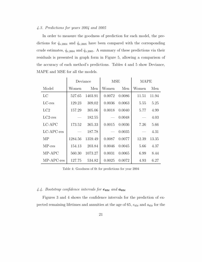
4.3. Predictions for years 2004 and 2005

In order to measure the goodness of prediction for each model, the pre-

dictions for qx,2004 and qx,2005 have been compared with the corresponding

crude estimates, qx,2004 and qx,2005. A summary of these predictions via their

residuals is presented in graph form in Figure 5, allowing a comparison of

the accuracy of each method’s predictions. Tables 4 and 5 show Deviance,

MAPE and MSE for all the models.

Deviance MSE MAPE

Model Women Men Women Men Women Men

LC 527.65 1403.91 0.0072 0.0086 11.51 11.94

LC-res 129.23 309,02 0.0036 0.0063 5.55 5.25

LC2 157.29 305.06 0.0018 0.0040 5.77 4.99

LC2-res — 182.55 — 0.0048 — 4.03

LC-APC 173.52 365.33 0.0015 0.0036 7.26 5.66

LC-APC-res — 187.78 — 0.0035 — 4.31

MP 1284.56 1359.49 0.0087 0.0077 12.39 13.35

MP-res 154.13 203.84 0.0046 0.0045 5.66 4.37

MP-APC 560.30 1073.27 0.0031 0.0065 6.99 8.44

MP-APC-res 127.75 534.82 0.0025 0.0072 4.93 6.27

Table 4: Goodness of fit for predictions for year 2004

4.4. Bootstrap confidence intervals for e65t and a65t

Figures 3 and 4 shows the confidence intervals for the prediction of ex-

pected remaining lifetimes and annuities at the age of 65, e65t and a65t for the

21

Deviance MSE MAPE

Model Women Men Women Men Women Men

LC 883.46 2091.91 0.0096 0.0110 14.30 15.53

LC-res 383.55 804.47 0.0053 0.0050 8.92 9.39

LC2 324.48 545.71 0.0035 0.0054 7.52 6.46

LC2-res — 512.03 — 0.0050 — 6.11

LC-APC 330.00 725.91 0.0029 0.0054 8.81 7.95

LC-APC-res — 675.67 — 0.0065 — 7.08

MP 1210.48 1472.71 0.0075 0.0066 14.61 15.37

MP-res 386.56 697.87 0.0049 0.0062 8.71 8.51

MP-APC 457.55 1275.27 0.0024 0.0069 7.66 10.58

MP-APC-res 205.96 644.92 0.0022 0.0074 6.15 7.85

Table 5: Goodness of fit for predictions for year 2005

period 2004-2023 obtained with different models using bootstrap techniques

described in Section 3. For the left-hand graphs only the model trends have

been used (only trend), and in the right-hand ones the model includes the

adjustment of residuals through geostatistical methods (trend + res).

We can see that, in general, the expected remaining lifetime is higher for

women than for men and there is a clear increasing in e65t over the time.

This fact is true for both trend and geostatistics intervals, which show a very

similar rank values for the predicted period.

Moreover, it can be seen that the MP model provides higher values for

expectancy, which is due to the prediction of a reduction in the qxt for all

ages while the other models predict increases for the advanced and interme-

22

diate age groups, although these latter do not figure in the calculation of e65t.

We should also point out the lower value of the predictions of e65t obtained

with the LC-APC model compared with those provided by the classic Lee-

Carter, LC, due to the fact that the cohorts figuring in the obtaining of the

predictions increase the values of the mortality ratios. Renshaw and Haber-

man (2006) observe just the opposite for the mortality data for England and

Wales, and we believe that the explanation for this apparent contradiction

may be the distinct behaviour of Spanish mortality.

With regard to the width of the intervals, as a general observation what

stands out is the narrowness of trend intervals, a feature in common with

other published studies (Lee and Carter, 1992; Lee, 2000; Booth et al., 2002;

Koissi et al., 2006) whose authors offer different explanations for it. In the

paper by Li, Hardy y Tan (2006) the phenomenon is attributed to the rigidity

of the Lee-Carter model structure and to avoid it they relax that structure

by incorporating the heterogeneity from each age-period cell. As far as the

influence of gender and of the model over it, there does not seem to be a

clear effect of either factor when they are considered separately. We could

speak, nonetheless, of the existence of an interaction between them both. For

example, the greatest amplitude of intervals for the MP model for men moves

to the LC-APC model for women. This comment is as valid for expected

remaining lifetime as it is for the annuities. The intervals obtained with

trend + res models show wider and more irregular intervals.

If we compare with similar studies carried out using Spanish mortal-

ity data, our results are slightly higher than those obtained by Guillen and

Vidiella-i-Anguera (2005), though only in the case of expected remaining

23

lifetime because, as we point out in the Introduction, we have not found

precedents for a similar study for annuities. From these we can say that, in

general, they are also higher for women than for men, in concordance with

the fact that those have a higher expected remaining lifetime.

2005 2010 2015 2020

11.0

12.0

13.0

14.0

MEN only trend

a 65t

LCLC−APCMP

2005 2010 2015 2020

11.0

12.0

13.0

14.0

MEN trend + res

a 65t

LCLC−APCMP

2005 2010 2015 2020

13.0

14.0

15.0

16.0

WOMEN only trend

a 65t

LCLC−APCMP

2005 2010 2015 2020

13.0

14.0

15.0

16.0

WOMEN trend + res

a 65t

LCMP

Figure 3: Bootstrap interval for e65t for men and women.

5. Conclusions

5.1. Model fitting

Table 3 shows the goodness of fit values for different adjustments. A

first conclusion, common to all models, is that adjustments perform better

24

2005 2010 2015 2020

11.0

12.0

13.0

14.0

MEN trends

a 65t

LCLC−APCMP

2005 2010 2015 2020

11.0

12.0

13.0

14.0

MEN geo

a 65t

LCLC−APCMP

2005 2010 2015 2020

13.0

14.0

15.0

16.0

WOMEN trends

a 65t

LCLC−APCMP

2005 2010 2015 2020

13.0

14.0

15.0

16.0

WOMEN geo

a 65t

LCMP

Figure 4: Bootstrap interval for a65t for men and women.

for women than for men. This may be due to the fact that male mortality

fluctuations for the ages in the accident hump are difficult to capture over

the period of time under consideration.

The LC-APC model shows the best global result for both sexes and for

the goodness-of-fit measures. The explanation of this can be found in the

introduction of the cohort effect. In general, the inclusion of the cohort effect

improves the models. It is worth highlighting two points: the practical disap-

pearance in the second of the diagonal pattern which can be seen in the first,

attributable to a cohort effect, and the reduction in error for intermediate

25

and advanced age-groups.

5.2. Future prediction

Tables 4 and 5 show the results for all prediction models and also now,

the first and immediate conclusion is that mortality is predicted better for

women than for men.

The Geostatistical models, when applied, improve the results for both

years. This improvement is pronounced for simpler models, the Lee-Carter

with one term (LC) and the Media-Polish without cohort effect (MP). The

LC2 and LC-APC models for women show a good performance. The expla-

nation of this can be found in the introduction of the second term which

adapts the model better for the ages involved in the accident hump (Debon

et al., 2008) and for advanced and intermediate ages. In particular, the inclu-

sion of a cohort effect improves the prediction. This better behaviour makes

unnecessary to resort to geostatistics in order to model the corresponding

residuals.

The greatest differences between the crude and predicted values are ob-

served in the intermediate ages. This fact is clearly shown in Figure 5, which

specifies the magnitude of residuals for all ages and models. This figure also

confirms the point in the above paragraph.

A comment must be made with regard to the MP-APC model. Although

it is not the model which produces the best global results, it has in its favour

that its parameters are easily interpretable in as much as they describe the

evolution of mortality over age, period and cohort, its computational cost is

very low and it is a robust model up against the outliers. For these reasons, we

think that this type of model must be borne in mind for future development.

26

Men 2004

age

0.1

0.2

0.3

0.4

0.5

LC res LC2 res LC−APC res MP res MP−APC res

1020

3040

5060

7080

90

Women 2004

age

0.1

0.2

0.3

0.4

0.5

0.6

LC res LC2 LC−APC MP res MP−APC res

1020

3040

5060

7080

90

Men 2005

age

0.1

0.2

0.3

0.4

0.5

LC res LC2 res LC−APC res MP res MP−APC res

1020

3040

5060

7080

90

Women 2005

age

0.1

0.2

0.3

0.4

0.5

LC res LC2 LC−APC MP res MP−APC res

1020

3040

5060

7080

90Figure 5: Absolute values of prediction residuals for each age for different models.

5.3. A final comment

From the preceding conclusions it can be deduced that the model with

the best fit is not always the one that predicts best as, for example, the LC2

model, which generally predicts better than the LC-APC model. As Tabeau

et al. (2001) affirm, good modelling is necessary for getting predictions but

it does not always guarantee that these are good. On the other hand, it

should be noted that in spite of a higher computational cost, LC-APC and

the Geostatistical models have still a favourable cost/benefit ratio.

We must emphasise again the narrowness of the bootstrap confidence in-

tervals obtained for expected remaining lifetime and for the annuities. Apart

from the comments that this attracts from some authors and which we have

referred to in Section 4.4, it can be used to deduce that the possible fluctu-

27

ations in mortality ratios are not reflected in those two measures.

Appendix A. Lee-Carter model fitting

First of all, it should be pointed out that the models cannot be adjusted

through normal regression methods because the values of ku1and ku2

cannot

be observed. The gnm library of the R Development Core Team (2005),

developed by Turner and Firth (2006), allows adjustment. We have adapted

the code written by the authors to adjust the force of mortality, µxt, under

a Poisson distribution and log link, to the adjustment of the probability of

death, qxt, under the Binomial distribution and logit link. In particular, its

gnm function allows us to obtain generalised linear models with multilinear

terms through the Mult function.

The Lee-Carter models present problems of identifiability, given a solution

of (2), (ax, bx, kt), any transformation of the type (ax, bx/c, ckt) or (ax +

cbx, bx, kt − c), ∀c, is also a solution. In order to avoid this difficulty and to

get a single solution, some constraints must be imposed to the parameters.

Lee and Carter (1992) propose the normalization∑

x

bx = 1 and∑

t

kt = 0.

The Lee-Carter model with two time terms interacting with age, model

LC2 in Table 1, can be adjusted with the gnm library using the instances

function. The problem of identifiability in the model can be resolved with

the restrictions∑

x

b1x = 1 and

∑

t

k1t = 0,

∑

x

b2x = 1,

∑

t

k2t = 0.

The Lee-Carter model with age-period-cohort effect, model LC-APC in

Table 1, presents adjustment problems due to the relationship between two

factors, cohort = year − age. Renshaw and Haberman (2006) propose car-

rying the estimation out in two stages. First, ax is adjusted in accordance

28

with the original version by Lee-Carter,

ax =

∑

t

ln

(

qxt

1 − qxt

)

T. (A.1)

Thereafter, the remaining parameters can be adjusted with the values of

ax fixed through the offset term. To resolve the problem of identifiability, the

authors consider the following restrictions∑

x

b1x = 1,

∑

x

b2x = 1 and kt1 =

0 or kc1 = 0, with t1 and c1 being the first period and and first cohort,

respectively. In line with our experience, the choice of period or origin cohort

influences the convergence of the algorithm. It is worth choosing t0 or c0 in

such a way that the behaviour of the logit(qxt0) is as similar as possible to

the estimations (A.1).

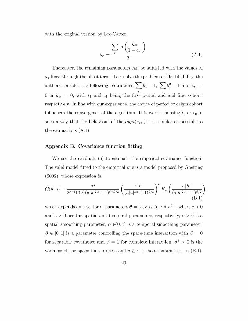
Appendix B. Covariance function fitting

We use the residuals (6) to estimate the empirical covariance function.

The valid model fitted to the empirical one is a model proposed by Gneiting

(2002), whose expression is

C(h, u) =σ2

2ν−1Γ(ν)(a|u|2α + 1)δ+β/2

(

c‖h‖

(a|u|2α + 1)β/2

)ν

Kν

(

c‖h‖

(a|u|2α + 1)β/2

)

,

(B.1)

which depends on a vector of parameters θ = (a, c, α, β, ν, δ, σ2)′, where c > 0

and a > 0 are the spatial and temporal parameters, respectively, ν > 0 is a

spatial smoothing parameter, α ∈]0, 1] is a temporal smoothing parameter,

β ∈ [0, 1] is a parameter controlling the space-time interaction with β = 0

for separable covariance and β = 1 for complete interaction, σ2 > 0 is the

variance of the space-time process and δ ≥ 0 a shape parameter. In (B.1),

29

Kν is the modified Bessel function of the second kind of order ν (Abramowitz

and Stegun, 1965).

The choice of this covariance function model is motivated by its flexibility

for adjustment. Theoretical details and properties of this class of covariance

functions can be found in Martınez-Ruiz (2008).

Acknowledgments

This work was partially supported by grants from the MEyC (Minis-

terio de Educacion y Ciencia, Spain, project MTM2007-62923 and project

MTM2008-05152). The research by Ana Debon and Francisco Martınez-Ruiz

has also been partially supported by a grant from the Generalitat Valenciana

(grant No. GVPRE/2008/103).

References

Abramowitz, M. and Stegun, I. A. (1965). Handbook of Mathematical Func-

tions. Dover, New York.

Benjamin, B. and Soliman, A. (1993). Mortality on the Move. Actuarial

Education Service, Oxford.

Booth, H., Hyndman, R., Tickle, L., and de Jong, P. (2006). Lee-Carter mor-

tality forecasting: a multi-country comparison of variants and extensions.

Demographic Research, 15(9):289–310.

Booth, H., Maindonald, J., and Smith, L. (2002). Applying Lee-Carter under

conditions of variable mortality decline. Population Studies, 56(3):325–336.

30

Cressie, N. (1993). Statistics for Spatial Data, Revised Edition. John Wiley,

New York.

Cressie, N. and Majure, J. (1997). Spatio-temporal statistical modelling of

livestock waste in streams. Journal of Agricultural, Biological, and Envi-

ronmental Statistics, 2(1):24–47.

Debon, A., Montes, F., and Puig, F. (2008). Modelling and forecasting

mortality in Spain. European Journal of Operation Research, 189(3):624–

637.

Debon, A., Montes, F., and Sala, R. (2005). A comparison of parametric

models for mortality graduation. Application to mortality data of the Va-

lencia region (Spain). Statistics and Operations Research Transactions,

29(2):269–287.

Debon, A., Montes, F., and Sala, R. (2006a). A comparison of models for

dinamical life tables. Application to mortality data of the Valencia region

(Spain). Lifetime data analysis, 12(2):223–244.

Debon, A., Montes, F., and Sala, R. (2006b). A comparison of nonparamet-

ric methods in the graduation of mortality: application to data from the

Valencia region (Spain). International Statistical Review, 74(2):215–233.

Brouhns, N., Denuit, M., and Keilegom, I. V. (2005). Bootstrapping Pois-

son log-bilinear model for mortality forecasting. Scandinavian Actuarial

Journal, (3):212–224.

Efron, B. y Tibshirani, R. (1993). An introduction to the boostrap. Chapman

& Hall, New York & London.

31

Felipe, A., Guillen, M., and Perez-Marın, A. (2002). Recent mortality trends

in the Spanish population. British Actuarial Journal, 8(4):757–786.

Forfar, D., McCutcheon, J., and Wilkie, A. (1988). On graduation by math-

ematical formula. Journal of the Institute of Actuaries, 115 part I(459):1–

149.

Gavin, J., Haberman, S., and Verrall, R. (1993). Moving weighted average

graduation using kernel estimation. Insurance: Mathematics & Economics,

12(2):113–126.

Gavin, J., Haberman, S., and Verrall, R. (1994). On the choice of bandwidth

for kernel graduation. Journal of the Institute of Actuaries, 121:119–134.

Gavin, J., Haberman, S., and Verrall, R. (1995). Graduation by kernel and

adaptive kernel methods with a boundary correction. Transactions. Society

of Actuaries, XLVII:173–209.

Gneiting, T. (2002). Nonseparable, stationary covariance functions for space-

time data. Journal of the American Statistical Association, 97:590–600.

Guillen, M. and Vidiella-i-Anguera, A. (2005). Forecasting Spanish natural

life expectancy. Risk Analysis, 25(5):1161–1170.

Hyndman, R. J. (2008). forecast: Forecasting functions for time series. R

package version 1.11.

Journel, A. G. and Huijbregts, C. J. (1978). Mining Geoestatistics. Academic

Press, New York.

32

Koissi, M., Shapiro, A., and Hognas, G. (2006). Evaluating and extending the

Lee-Carter model for mortality forecasting confidence interval. Insurance:

Mathematics & Economics, 38(1):1–20.

Lee, R. (2000). The Lee-Carter method for forecasting mortality, with various

extensions and applications. North American Actuarial Journal, 4(1):80–

91.

Lee, R. and Carter, L. (1992). Modelling and forecasting U. S. mortality.

Journal of the American Statistical Association, 87(419):659–671.

Li, S.-H., Hardy, M., y Tan, K. (2006). Uncertainty in mortality forecast-

ing: an extension to the classical Lee-Carter approach. Technical report,

Waterloo University.

Martınez-Ruiz, F. (2008). Modelizacion de la funcion de covarianza en pro-

cesos espacio-temporales: analisis y aplicaciones. PhD thesis, Universitat

de Valencia, Spain.

Mateu, J., Montes, F. and Plaza, M. (2004). The 1970 US draft lottery

revisited: a spatial analysis. JRSS Series C (Applied Statistics), 53(1):219–

229.

Matheron, G. (1975). Random Sets and Integral Geometry. Wiley, New York.

Pedroza, C. (2006). A bayesian forecasting model: predicting U.S. male

mortality. Biostatistics, 7(4):530–550.

Pitacco, E. (2004). Survival models in dynamic context: a survey. Insurance:

Mathematics & Economics, 35(2):279–298.

33

R Development Core Team (2005). R: A Language and Environment for

Statistical Computing. R Foundation for Statistical Computing, Vienna,

Austria. ISBN 3-900051-07-0.

Renshaw, A. (1991). Actuarial graduation practice and generalised linear

models. Journal of the Institute of Actuaries, 118(II):295–312.

Renshaw, A. and Haberman, S. (2003). Lee-Carter mortality forecasting

with age specific enhancement. Insurance: Mathematics & Economics,

33(2):255–272.

Renshaw, A. and Haberman, S. (2006). A cohort-based extension to the

Lee-Carter model for mortality reduction factors. Insurance: Mathematics

& Economics, (3):556–570.

Renshaw, A. and Haberman, S. (2008). On simulation-based approaches to

risk measurement in mortality with specific reference to poisson Lee-Carter

modelling. Insurance: Mathematics & Economics, 42(2):797–816.

Tabeau, E., van den Berg Jeths, A. and Heathcote (Eds), C. (2001). A

Review of Demographic Forecasting Models for Mortality. Forecasting in

Developed Countries: From description to explanation. Kluwer Academic

Publishers.

Turner, H. and Firth, D. (2006). Generalized nonlinear models in R: An

overview of the gnm package. R package version 0.9-1.

Wong-Fupuy, C. and Haberman, S. (2004). Projecting mortality trends:

Recent developents in the United Kingdom and the United States. North

American Actuarial Journal, 8(2):56–83.

34