A GENETIC ALGORITHM ENHANCED BY DOMINANCE … · A GENETIC ALGORITHM ENHANCED BY DOMINANCE...

International Journal of InnovativeComputing, Information and Control ICIC International c⃝2011 ISSN 1349-4198Volume 7, Number 5(A), May 2011 pp. 2323–2343

A GENETIC ALGORITHM ENHANCED BY DOMINANCEPROPERTIES FOR SINGLE MACHINE SCHEDULING

PROBLEMS WITH SETUP COSTS

Pei-Chann Chang1, Shih-Hsin Chen2, Ting Lie1 and Julie Yu-Chih Liu1

1Department of Information ManagementYuan-Ze University

No. 135, Yuan-Dong Road, Taoyuan 32026, Taiwan{ iepchang; tinglie; imyuchih }@saturn.yzu.edu.tw

2Department of Electronic Commerce ManagementNanhua University

No. 32, Chungkeng, Dalin, Chiayi 62248, [email protected]

Received January 2010; revised May 2010

Abstract. This paper considers a single machine scheduling problem in which n jobsare to be processed and a machine setup time is required when the machine switches jobsfrom one to the other. All jobs have a common due date that has been predeterminedusing the median of the set of sequenced jobs. The objective is to find an optimal sequenceof the set of n jobs to minimize the sum of the job’s setups and the cost of tardy orearly jobs related to the common due date. In this research, dominance properties aredeveloped by swapping the neighborhood jobs. The time complexity of the dominanceproperties is in O(n2) and it is very efficient when combined with the GA. To preventearlier convergence of a Simple Genetic Algorithm (SGA), these dominance propertiesare further embedded in SGA to improve the efficiency and effectiveness of the globalsearching procedure. Analytical results in benchmark problems are presented and thecomputational algorithms are developed.

1. Introduction. Single-machine scheduling problems are one of the well-studied prob-lems by many researchers. The application of single machine scheduling with setups canbe found in minimizing the cycle time for pick and place (PAP) operations in PrintedCircuit Board manufacturing company [24]; in a steel wire factory in China [22] and a se-quencing problem in the weaving industry [2]. The results developed in the literature notonly provide the insights into the single machine problem but also for more complicatedenvironment such as flow shop or job shop.

The problem considered in this paper is to schedule a set of n jobs {j1, j2, · · · , jn} on asingle machine that is capable of processing only one job at a time without preemption.As explained in [6,30], all jobs are available at time zero, and a job j requires a processingtime Pj. Job j belongs to a group gj ∈ {1, . . . , q} (with q ≤ n). Setup or changeovertimes, which are given as two q × q matrices, are associated to these groups. This meansthat in a schedule where jj is processed immediately after ji where i, j ∈ {1, 2, · · · , n},there must be a setup time of at least Sij time units between the completion time of ji,denoted by Ci, and the start time of jj, which is Cj − Pj. During this setup period, noother task can be performed by the machine and we assume that the cost of the setupoperation is c (gi; gj) ≥ 0 and let it be equal to Machine setup time Sij which is includedas sequence dependent. The objective is to complete all the jobs as close as possible to a

2323

2324 P.-C. CHANG, S.-H. CHEN, T. LIE AND J. Y.-C. LIU

large, common due date d. To accomplish this objective, the summation of earliness andtardiness is minimized. The earliness of job j is denoted as Ej = max (0, d− Cj) and itstardiness as Tj = max (Cj − d, 0), where Cj is the completion time of job j. Earliness andtardiness penalties for job j are weighted equally. The objective function is given by

minZ =n∑

j=1

(Ej + Tj) =n∑

j=1

|d− Cj| (1)

The inclusion of both earliness and tardiness costs in the objective function is compat-ible with the philosophy of just-in-time production, which emphasizes producing goodsonly when they are needed. The early cost may represent the cost of completing a productearly, the deterioration cost for a perishable goods or a holding (stock) cost for finishedgoods. The tardy cost can represent rush shipping costs, lost sales and loss of goodwill.Some specific examples of production settings with these characteristics are provided by[28,31,32,34]. The set of jobs is assumed to be ready for processing at the beginning whichis a characteristic of the deterministic problem. The set of jobs is assumed to be ready forprocessing at the beginning which is a characteristic of the deterministic problem. As ageneralization of weighted tardiness scheduling, the problem is strongly NP-hard in [25].Consequently, the early/tardy problem is also a strong NP-hard problem.The single-machine E/T problem was first introduced by [23]. Since then many re-

searchers worked on various extensions of the problem. Baker and Scudder [6] publisheda comprehensive state-of-the-art review for different versions of the E/T problem. Kanet[23] examined the E/T problem with equal penalties and unrestricted common due date.A problem is considered unrestricted when the due date is large enough not to constrainthe scheduling process. He introduced a polynomial-time algorithm to solve the problemoptimally. Hall et al. [18] extended Kanet’s work and developed an algorithm that findsa set of optimal solutions for the problem based on some optimality conditions. Hall andPosner [19] solved the weighted version of the problem with no setup times. Azizogluand Webster [4] introduced a Branch-and-Bound algorithm to solve the problem withsetup times; however, they assumed that setup times are not sequence dependent. Otherresearchers worked on the same problem but with a restricted due date (see for example[1,5,14,19,26,27]). Other interesting applications of scheduling problems with intelligentapproaches can also be found in [20,21,29,30,33].In most of the E/T literature, it has been assumed that no setup time is required. In

many realistic situations, however, setup times are needed and are sequence-dependent.In general, scheduling problems with sequence-dependent setup times are similar to thetraveling salesman problem (TSP) in [16], which is also NP-hard [25]. Coleman [15]presented a 0/1 mixed integer programming model (MIP) for the single-machine E/Tproblem with job-dependent penalties, distinct due dates and sequence-dependent setuptimes. Coleman’s work was one of the few papers that dealt with the E/T problem withsequence-dependent setup times, but for a small number of jobs. Chen [13] addressed theE/T problem with batch sequence-dependent setup times. He showed that the problemwith unequal penalties is NP-hard even when there are only two batches of jobs and twodue dates that are unrestrictedly large. Allahverdi et al. [3] reviewed the scheduling lit-erature that involved setup times. In their review, very few papers addressed the E/Tproblem with setup times, and no paper tackled the problem addressed in this researchwith the development of dominance properties. Application of Genetic Algorithm (GA)in various scheduling problems can be referred in [7-12], however, as observed by mostresearchers, the simple GA will be trapped into local optimality in the earlier stages andcannot be converged into global optimal in most of the cases. The problems with the

A GA WITH DOMINANCE PROPERTY FOR SMS WITH SETUP COSTS 2325

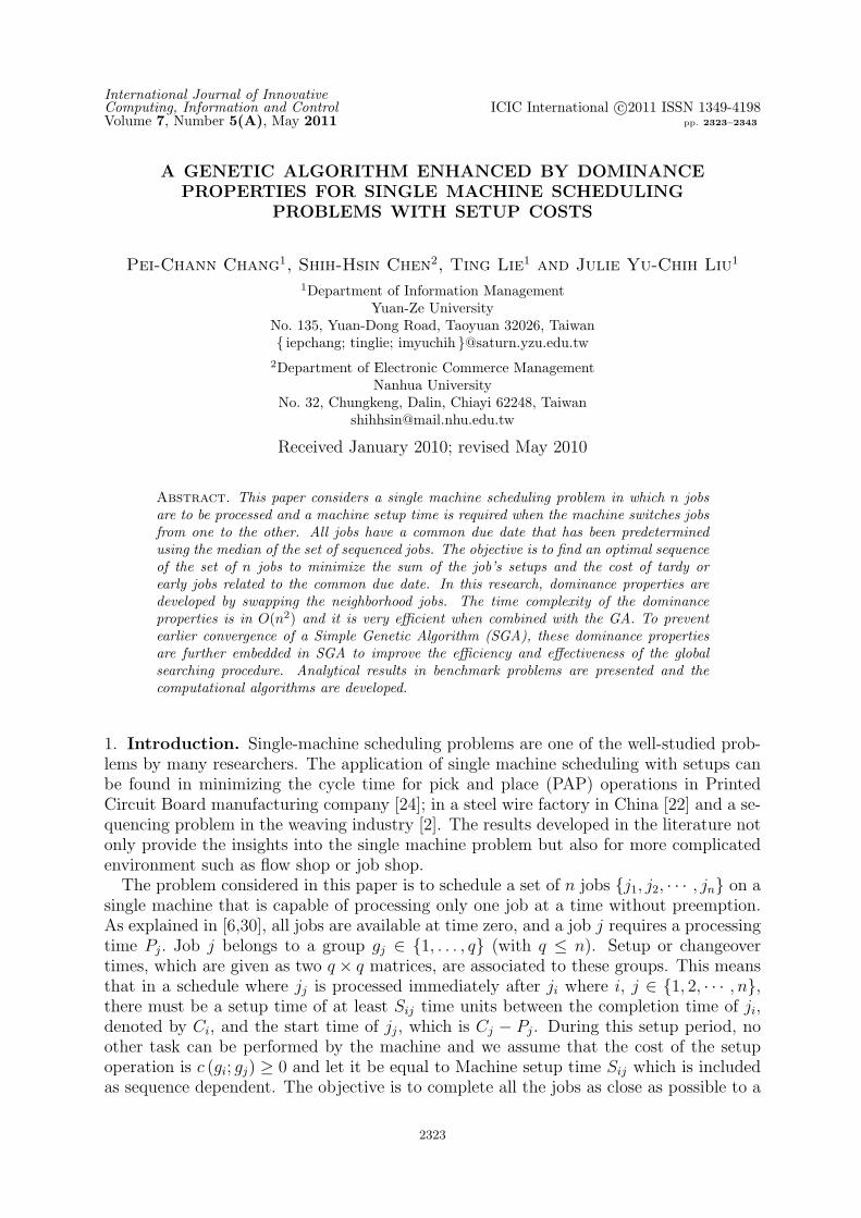
Figure 1. The total earliness and total tardiness for a pre-assigned due-date d

steady states GAs having premature convergence led to the desire to further improvethe convergence of the algorithm. Therefore, in this research, dominance properties aredeveloped according to the sequence swapping of two neighborhood jobs and these dom-inance properties are further embedded in the Simple Genetic Algorithm to improve theefficiency and effectiveness of the global searching procedure. The time complexity of thedominance properties is in O(n2) and it is very efficient when combined with the GA.

2. Problem Statements. We consider the sequence-dependent scheduling problem witha common due date. The common due date model corresponds; for instance, to anassembly system in which the components of the product should be ready at the sametime, or to a shop where several jobs constitute a single customer’s order in [17]. It isshown in [23] that an optimal sequence in which the b-th job is completed at the due-date.The value of b is given by:

b =

{n/2 if n is even(n+ 1)/2 if n is odd

(2)

The common due-date (k∗) is the sum of processing times of jobs in the first b positionsin the sequence; i.e.,

k∗ = Cb (3)

As soon as the common due date is assigned, see Figure 1, jobs can be classified intotwo groups that are early and tardy which are at position from 1 to b and b + 1 to nrespectively. The following notations are employed in the latter section.

[j]: job in position j;A: the job set of tardy jobs;B: the job set of early jobs;AP[j][j+1]: Adjusted processing time for the job in position j followed by the job in

position [j + 1];b: the median position;AP[j][j+1] is actually the processing time of job j+1 with setup time. Thus, the original

form of AP[j][j+1] is S[j][j+1] + Pj+1.Our objective is to minimize the total earliness/tardiness cost. The formulation is given

below.

Minimize f(x) =n∑

i=1

(Ei + Ti) = TT + TE (4)

whereTT : Total tardiness for a job sequenceTE : Total earliness for a job sequence

TT =n−1∑j=b

(n− j)AP[j][j+1] (5)


(a) Adjacent interchange

(b) Nonadjacent interchange

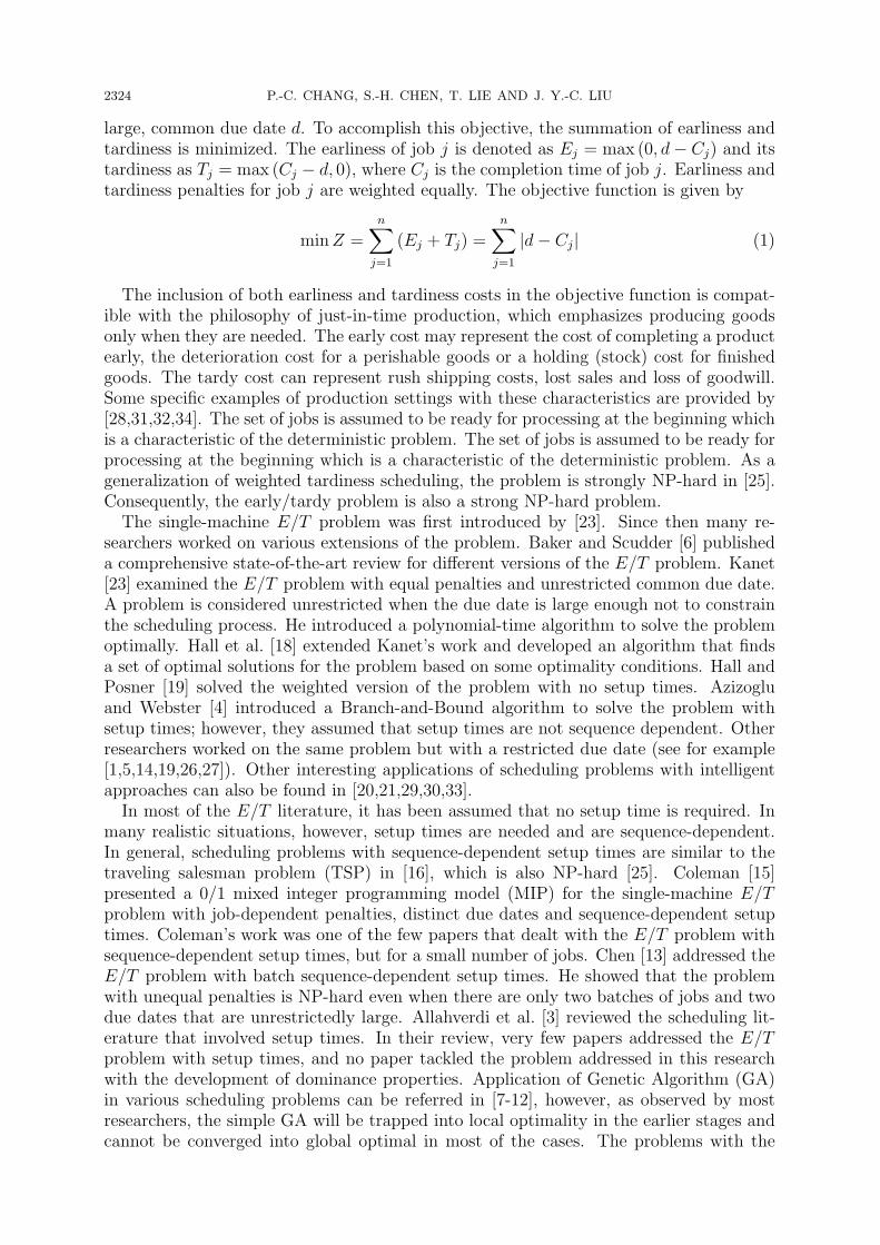
Figure 2. Two different types of interchanging methods

TE =b∑

j=1

(j − 1)AP[j−1][j] (6)

3. Derivations of Dominance Properties. We consider the problem of scheduling njobs in a single machine and derive the dominance properties (necessary conditions) of theoptimal schedule. In this section, we use the objective function (Z(

∏)) for total absolute

deviation for the schedule∏. To develop these dominance properties, we will consider

interchanging two adjacent jobs and nonadjacent jobs in the schedule, and prove someintermediate results. The adjacent interchange and nonadjacent interchange of job i andjob j are depicted in Figures 2(a) and 2(b) respectively.Thus, there are two schedules, i.e.,

∏X for scheduleX and

∏Y for the modified schedule

Y . The corresponding objective functions of∏

X and∏

Y , i.e., Z(∏

X) and Z(∏

Y ), arelisted as follows:

Z

(∏x

)= G1 +G2 +G3 (7)

Z

(∏y

)= G

′

1 +G′

2 +G′

3 (8)

where

1. G1: the objective of job(s) before job i;2. G2: the objective between job i and job j;3. G3: the objective of job(s) after job j;4. G

′1: the objective job(s) before job j;

5. G′2: the objective between job j and job i;

6. G′3: the objective of job(s) after job i.

We compare schedules∏

X and∏

Y by finding the conditions under which∏

X is betterthan

∏Y . For a pair of jobs, i.e., job i and job j in a schedule, no matter for adjacent

interchange or nonadjacent interchange, they are in one of the following status:

1. Job i is early and job j is early;2. Job i is early and job j is on-time;


Figure 3. Swapping job i and job j when both of them are adjacent and early

3. Job i is on-time and job j is tardy;4. Job i is tardy and job j is tardy.

Because the objective values of a schedule with adjacent or nonadjacent interchangeare different, there are totally 8 conditions corresponding to these two types of exchanges.Other than the cases discussed above, there is one extra case to be discussed in nonadjacentinterchange which is the following:

1. Job i is early and job j is tardy

According to the cases discussed above, there are four dominance properties for theadjacent interchange which are explained in Section 3.1 and five dominance properties forthe nonadjacent interchange which are shown in Section 3.2.

3.1. Dominance properties for adjacent interchange. When we exchange two adja-cent jobs as shown in Figure 3, the objective values of related jobs in position i, i+1 andi + 2 are changed while the others are still the same. These objective terms in positioni, i + 1 and i + 2 are different. Consequently, when we subtract Z(

∏Y ) from Z(

∏X),

redundant terms are reduced.

Lemma 3.1. In a given schedule∏

X , for any two adjacent jobs (job i and job j) areboth early, then the total deviation of Z(

∏Y ) is better than Z(

∏X) only when

(i− 1)(AP[i−1][j]) + (j − 1)(AP[j][i]) + (j)(AP[i][j+1])

≤ (i− 1)(AP[i−1][i]) + (j − 1)(AP[i][j]) + (j)(AP[j][j+1])

Proof: Figure 3 shows the relationships among these jobs.The difference of the objective between Z(

∏X) and Z(

∏Y ) are shown as follows:

∵ G1 =i−2∑k=1

(k − 1)AP[k][k+1]

G2 = (i− 1)AP[i−1][i] + (j − 1)AP[i][j]

G3 =b∑

k=j+1

(k − 1)AP[k−1][k] +n−1∑k=b

(n− k)AP[k][k+1]

G′

2 = (i− 1)AP[i−1][j] + (j − 1)AP[i][j]

G′

3 =b∑

k=i+1

(k − 1)AP[k−1][k] +n−1∑k=b

(n− k)AP[k][k+1]

To derive the condition under which Z(∏

X) ≥ Z(∏

Y ), the value of Z(∏

Y )− Z(∏

X)

is calculated. Let X = Z(∏

Y ) − Z(∏

X) and is equal to (G′2 − G2) + (G

′3 − G3). From

the above expression, we can derive the following:

(i− 1)(AP[i−1][j]) + (j − 1)(AP[j][i]) + (j)(AP[i][j+1])

≤ (i− 1)(AP[i−1][i]) + (j − 1)(AP[i][j]) + (j)(AP[j][j+1])


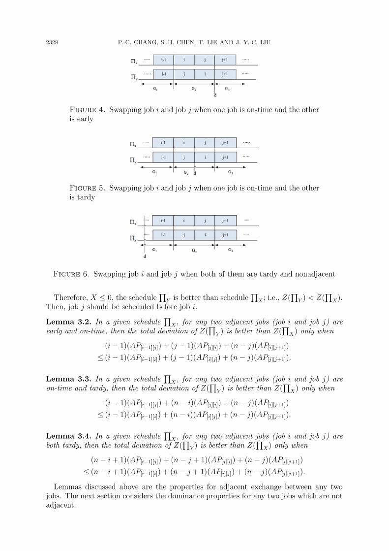
Figure 4. Swapping job i and job j when one job is on-time and the otheris early

Figure 5. Swapping job i and job j when one job is on-time and the otheris tardy

Figure 6. Swapping job i and job j when both of them are tardy and nonadjacent

Therefore, X ≤ 0, the schedule∏

Y is better than schedule∏

X ; i.e., Z(∏

Y ) < Z(∏

X).Then, job j should be scheduled before job i.


X , for any two adjacent jobs (job i and job j) areearly and on-time, then the total deviation of Z(


∏X) only when

(i− 1)(AP[i−1][j]) + (j − 1)(AP[j][i]) + (n− j)(AP[i][j+1])

≤ (i− 1)(AP[i−1][i]) + (j − 1)(AP[i][j]) + (n− j)(AP[j][j+1]).


X , for any two adjacent jobs (job i and job j) areon-time and tardy, then the total deviation of Z(


∏X) only when

(i− 1)(AP[i−1][j]) + (n− i)(AP[j][i]) + (n− j)(AP[i][j+1])

≤ (i− 1)(AP[i−1][i]) + (n− i)(AP[i][j]) + (n− j)(AP[j][j+1]).


X , for any two adjacent jobs (job i and job j) areboth tardy, then the total deviation of Z(


∏X) only when

(n− i+ 1)(AP[i−1][j]) + (n− j + 1)(AP[j][i]) + (n− j)(AP[i][j+1])

≤ (n− i+ 1)(AP[i−1][i]) + (n− j + 1)(AP[i][j]) + (n− j)(AP[j][j+1]).

Lemmas discussed above are the properties for adjacent exchange between any twojobs. The next section considers the dominance properties for any two jobs which are notadjacent.


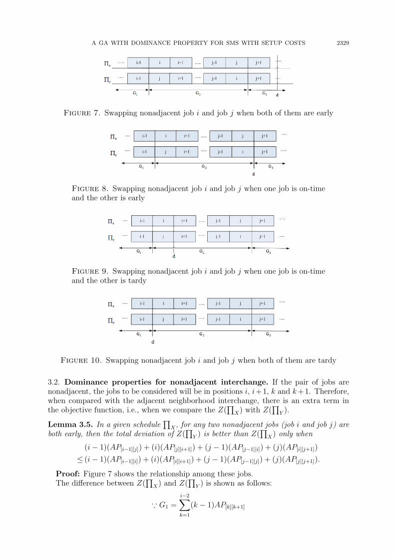
Figure 7. Swapping nonadjacent job i and job j when both of them are early

Figure 8. Swapping nonadjacent job i and job j when one job is on-timeand the other is early

Figure 9. Swapping nonadjacent job i and job j when one job is on-timeand the other is tardy

Figure 10. Swapping nonadjacent job i and job j when both of them are tardy

3.2. Dominance properties for nonadjacent interchange. If the pair of jobs arenonadjacent, the jobs to be considered will be in positions i, i+1, k and k+1. Therefore,when compared with the adjacent neighborhood interchange, there is an extra term inthe objective function, i.e., when we compare the Z(

∏X) with Z(

∏Y ).


X , for any two nonadjacent jobs (job i and job j) areboth early, then the total deviation of Z(


∏X) only when

(i− 1)(AP[i−1][j]) + (i)(AP[j][i+1]) + (j − 1)(AP[j−1][i]) + (j)(AP[i][j+1])

≤ (i− 1)(AP[i−1][i]) + (i)(AP[i][i+1]) + (j − 1)(AP[j−1][j]) + (j)(AP[j][j+1]).

Proof: Figure 7 shows the relationship among these jobs.The difference between Z(

∏X) and Z(

∏Y ) is shown as follows:

∵ G1 =i−2∑k=1

(k − 1)AP[k][k+1]


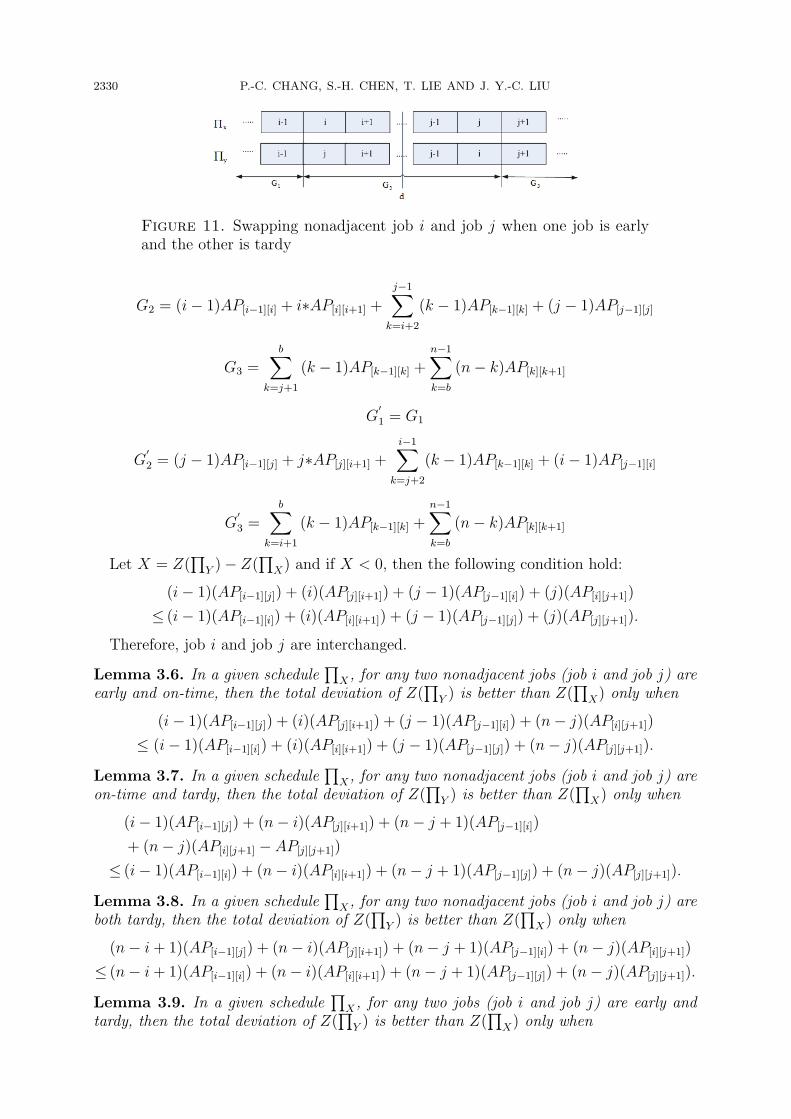
Figure 11. Swapping nonadjacent job i and job j when one job is earlyand the other is tardy

G2 = (i− 1)AP[i−1][i] + i∗AP[i][i+1] +

j−1∑k=i+2

(k − 1)AP[k−1][k] + (j − 1)AP[j−1][j]

G3 =b∑

k=j+1

(k − 1)AP[k−1][k] +n−1∑k=b

(n− k)AP[k][k+1]

G′

1 = G1

G′

2 = (j − 1)AP[i−1][j] + j∗AP[j][i+1] +i−1∑

k=j+2

(k − 1)AP[k−1][k] + (i− 1)AP[j−1][i]

G′

3 =b∑

k=i+1

(k − 1)AP[k−1][k] +n−1∑k=b

(n− k)AP[k][k+1]

Let X = Z(∏

Y )− Z(∏

X) and if X < 0, then the following condition hold:

(i− 1)(AP[i−1][j]) + (i)(AP[j][i+1]) + (j − 1)(AP[j−1][i]) + (j)(AP[i][j+1])

≤ (i− 1)(AP[i−1][i]) + (i)(AP[i][i+1]) + (j − 1)(AP[j−1][j]) + (j)(AP[j][j+1]).

Therefore, job i and job j are interchanged.


X , for any two nonadjacent jobs (job i and job j) areearly and on-time, then the total deviation of Z(


∏X) only when

(i− 1)(AP[i−1][j]) + (i)(AP[j][i+1]) + (j − 1)(AP[j−1][i]) + (n− j)(AP[i][j+1])

≤ (i− 1)(AP[i−1][i]) + (i)(AP[i][i+1]) + (j − 1)(AP[j−1][j]) + (n− j)(AP[j][j+1]).


X , for any two nonadjacent jobs (job i and job j) areon-time and tardy, then the total deviation of Z(


∏X) only when

(i− 1)(AP[i−1][j]) + (n− i)(AP[j][i+1]) + (n− j + 1)(AP[j−1][i])

+ (n− j)(AP[i][j+1] − AP[j][j+1])

≤ (i− 1)(AP[i−1][i]) + (n− i)(AP[i][i+1]) + (n− j + 1)(AP[j−1][j]) + (n− j)(AP[j][j+1]).


X , for any two nonadjacent jobs (job i and job j) areboth tardy, then the total deviation of Z(


∏X) only when

(n− i+ 1)(AP[i−1][j]) + (n− i)(AP[j][i+1]) + (n− j + 1)(AP[j−1][i]) + (n− j)(AP[i][j+1])

≤ (n− i+ 1)(AP[i−1][i]) + (n− i)(AP[i][i+1]) + (n− j + 1)(AP[j−1][j]) + (n− j)(AP[j][j+1]).


X , for any two jobs (job i and job j) are early andtardy, then the total deviation of Z(


∏X) only when


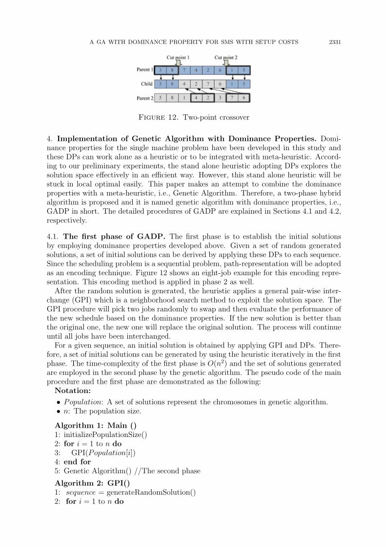
Figure 12. Two-point crossover

4. Implementation of Genetic Algorithm with Dominance Properties. Domi-nance properties for the single machine problem have been developed in this study andthese DPs can work alone as a heuristic or to be integrated with meta-heuristic. Accord-ing to our preliminary experiments, the stand alone heuristic adopting DPs explores thesolution space effectively in an efficient way. However, this stand alone heuristic will bestuck in local optimal easily. This paper makes an attempt to combine the dominanceproperties with a meta-heuristic, i.e., Genetic Algorithm. Therefore, a two-phase hybridalgorithm is proposed and it is named genetic algorithm with dominance properties, i.e.,GADP in short. The detailed procedures of GADP are explained in Sections 4.1 and 4.2,respectively.

4.1. The first phase of GADP. The first phase is to establish the initial solutionsby employing dominance properties developed above. Given a set of random generatedsolutions, a set of initial solutions can be derived by applying these DPs to each sequence.Since the scheduling problem is a sequential problem, path-representation will be adoptedas an encoding technique. Figure 12 shows an eight-job example for this encoding repre-sentation. This encoding method is applied in phase 2 as well.

After the random solution is generated, the heuristic applies a general pair-wise inter-change (GPI) which is a neighborhood search method to exploit the solution space. TheGPI procedure will pick two jobs randomly to swap and then evaluate the performance ofthe new schedule based on the dominance properties. If the new solution is better thanthe original one, the new one will replace the original solution. The process will continueuntil all jobs have been interchanged.

For a given sequence, an initial solution is obtained by applying GPI and DPs. There-fore, a set of initial solutions can be generated by using the heuristic iteratively in the firstphase. The time-complexity of the first phase is O(n2) and the set of solutions generatedare employed in the second phase by the genetic algorithm. The pseudo code of the mainprocedure and the first phase are demonstrated as the following:

Notation:

• Population: A set of solutions represent the chromosomes in genetic algorithm.• n: The population size.

Algorithm 1: Main ()1: initializePopulationSize()2: for i = 1 to n do3: GPI(Population[i])4: end for5: Genetic Algorithm() //The second phase

Algorithm 2: GPI()1: sequence = generateRandomSolution()2: for i = 1 to n do


3: for increment = 1 to 3 do4: for pos = 0 to n− increment do5: dominanceProperty(sequence, pos, pos+ increment)6: end for7: if sequence has not been changed then8: break;9: end if10: end for11: return sequence12: end for

4.2. The second phase of GADP. In the second phase, GA will be applied to furtherimprove the solution quality. The pseudo code of the genetic algorithm are listed asfollows:

Algorithm 3: Genetic Algorithm()1: Adopt the solutions from Phase 1()2: counter ← 03: while counter < maxGeneration do4: Evaluate Fitness()5: Elitism()6: Selection()7: Crossover()8: Mutation()9: counter ← counter+110: end while

The genetic operators applied in the Genetic Algorithm including the selection, crossoverand mutation operator will be explained in the following section.

4.2.1. Fitness and selection operator. Because the single machine scheduling with setupsis a single objective problem, the objective value of each chromosome can be used as fitnessdirectly. Then, the binary tournament selection is employed in the selection operation.The criterion to select better offspring is depended on their own fitness; the individualwhose fitness is better will be selected. As a result, the selection procedure selects betterchromosomes into the mating pool.

4.2.2. Crossover operator. The crossover procedure is randomly selecting two chromo-somes to mate. There are several crossover methods for combinatorial problem. Thisstudy employed the two-point crossover and the procedures of the two-point crossover arelisted as follows:

1. Select two chromosomes and named it as parent 1 and parent 2.2. Determine the two cut points, suppose they are at position i and j, copy the genes

which outside the range from i to j to the offspring in the same position.3. Copy the remaining genes which inside the range of parent 1 in the order of relative

gene position of parent 2.

4.2.3. Mutation. The purpose of mutation is to generate a new chromosome with a betterfitness by changing the gene position of the current chromosome. Swap mutation is appliedhere because it is easy to implement by setting two positions and exchanging the two valuesof these positions.


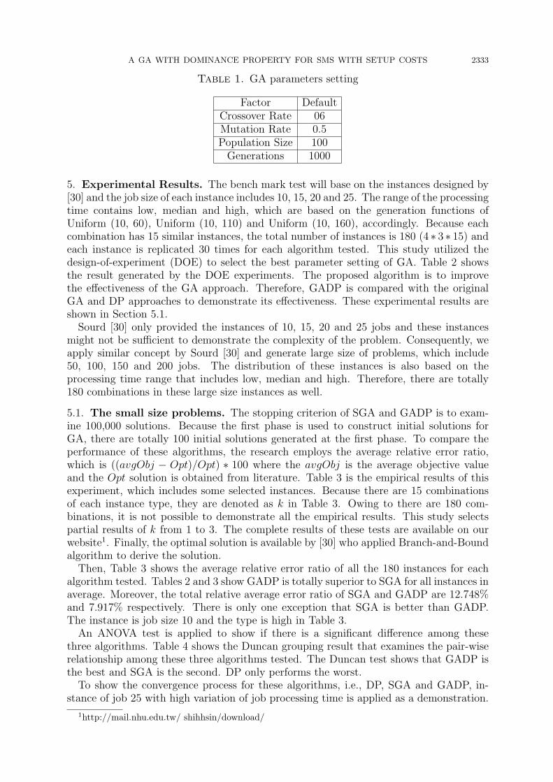
Table 1. GA parameters setting

Factor DefaultCrossover Rate 06Mutation Rate 0.5Population Size 100Generations 1000

5. Experimental Results. The bench mark test will base on the instances designed by[30] and the job size of each instance includes 10, 15, 20 and 25. The range of the processingtime contains low, median and high, which are based on the generation functions ofUniform (10, 60), Uniform (10, 110) and Uniform (10, 160), accordingly. Because eachcombination has 15 similar instances, the total number of instances is 180 (4 ∗ 3 ∗ 15) andeach instance is replicated 30 times for each algorithm tested. This study utilized thedesign-of-experiment (DOE) to select the best parameter setting of GA. Table 2 showsthe result generated by the DOE experiments. The proposed algorithm is to improvethe effectiveness of the GA approach. Therefore, GADP is compared with the originalGA and DP approaches to demonstrate its effectiveness. These experimental results areshown in Section 5.1.

Sourd [30] only provided the instances of 10, 15, 20 and 25 jobs and these instancesmight not be sufficient to demonstrate the complexity of the problem. Consequently, weapply similar concept by Sourd [30] and generate large size of problems, which include50, 100, 150 and 200 jobs. The distribution of these instances is also based on theprocessing time range that includes low, median and high. Therefore, there are totally180 combinations in these large size instances as well.

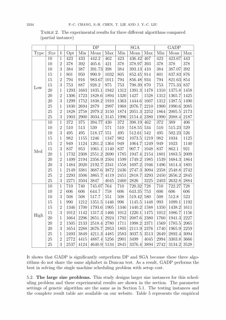
5.1. The small size problems. The stopping criterion of SGA and GADP is to exam-ine 100,000 solutions. Because the first phase is used to construct initial solutions forGA, there are totally 100 initial solutions generated at the first phase. To compare theperformance of these algorithms, the research employs the average relative error ratio,which is ((avgObj − Opt)/Opt) ∗ 100 where the avgObj is the average objective valueand the Opt solution is obtained from literature. Table 3 is the empirical results of thisexperiment, which includes some selected instances. Because there are 15 combinationsof each instance type, they are denoted as k in Table 3. Owing to there are 180 com-binations, it is not possible to demonstrate all the empirical results. This study selectspartial results of k from 1 to 3. The complete results of these tests are available on ourwebsite1. Finally, the optimal solution is available by [30] who applied Branch-and-Boundalgorithm to derive the solution.

Then, Table 3 shows the average relative error ratio of all the 180 instances for eachalgorithm tested. Tables 2 and 3 show GADP is totally superior to SGA for all instances inaverage. Moreover, the total relative average error ratio of SGA and GADP are 12.748%and 7.917% respectively. There is only one exception that SGA is better than GADP.The instance is job size 10 and the type is high in Table 3.

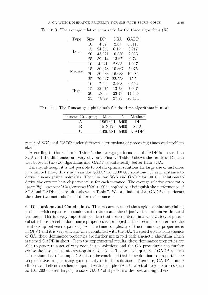
An ANOVA test is applied to show if there is a significant difference among thesethree algorithms. Table 4 shows the Duncan grouping result that examines the pair-wiserelationship among these three algorithms tested. The Duncan test shows that GADP isthe best and SGA is the second. DP only performs the worst.

To show the convergence process for these algorithms, i.e., DP, SGA and GADP, in-stance of job 25 with high variation of job processing time is applied as a demonstration.

1http://mail.nhu.edu.tw/ shihhsin/download/


Table 2. The experimental results for three different algorithms compared(partial instance)

DP SGA GADPType Size k Opt Min Mean Max Min Mean Max Min Mean Max

Low

101010151515202020252525

123123123123

423378384801794753129313061299183018281903

433392387950916887168317231752269427582900

442.2405.6391.73990.9983.67928.21835.11828.61838.228792979.23034.1

46242139810321011975194218941910299731503145

423378384805794753131213201363196818741996

436.42378.97393.13852.45856.48798.391391.314271444.62076.72051.32154.4

467393410914934870147815281607221022522380

423378384801794753131013121312190018641990

423.67378387.07837.83821.63775.331375.81365.71387.51990.62005.52088.4

443378392876854837145814251490208521732187

Med

101010151515202020252525

123123123123

372510495982949837173214991484214922932271

37551349511551124953230821942020338135063504

394.77539518.1712461261.21061.12551.22356.92192.73687.63865.73847

430571551134713641140269025042341387241194045

372510495982949837178515991558243624512460

398.19518.55512.611073.51064.7907.71947.41749.21697.22747.32818.72826

462534542121912491048215419851946309432933225

372510495982949837180115391496235824502403

389515.23502.2310341023862.11883.51684.31614.42548.82656.22632.8

40652952611251140921200918641801274228452884

High

101010151515202020252525

123123123123

71060650899013461012166415051654249327722537

740606508121217001142229621332288384944154124

745.07644.7517.71351.51793.61317.32651.12518.42676.74211.34887.44640.9

764758551144619051466292427802953448552565134

71060650899613461012179217111805258329012845

720.32643.35519.421145.51440.21220.12087.61998.22111.93037.534993376.4

728753580144815881475238023712376351340453894

71060650899313501012176015691740264929942742

722.27606512.81099.11438.21086.71941.31785.51965.92892.43303.83134.2

728606523119216111156222720652259309436663528

It shows that GADP is significantly outperform DP and SGA because these three algo-rithms do not share the same alphabet in Duncan test. As a result, GADP performs thebest in solving the single machine scheduling problem with setup cost.

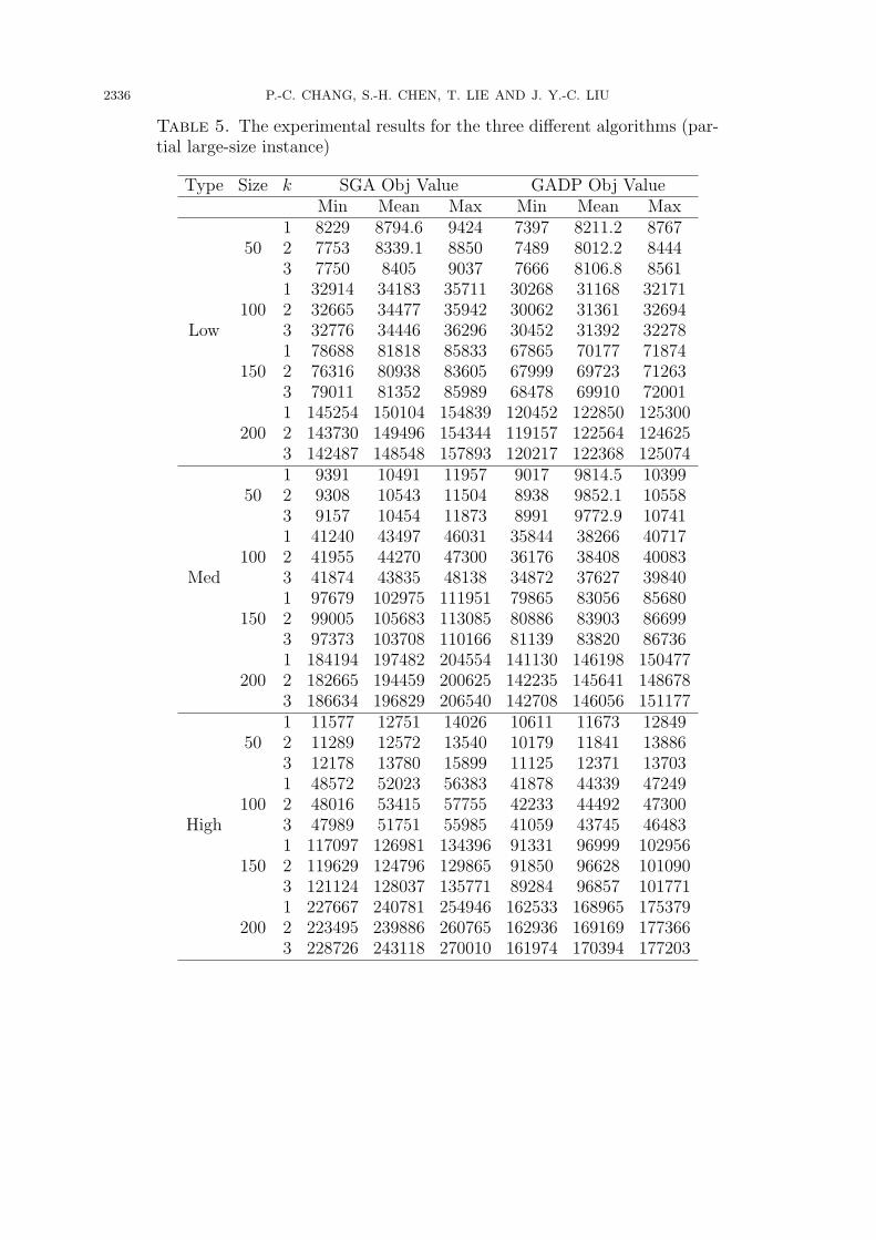
5.2. The large size problems. This study designs larger size instances for this sched-uling problem and these experimental results are shown in the section. The parametersettings of genetic algorithm are the same as in Section 5.1. The testing instances andthe complete result table are available on our website. Table 5 represents the empirical


Table 3. The average relative error ratio for the three algorithms (%)

Type Size DP SGA GADP

Low

10 4.32 2.07 0.311715 24.345 6.177 3.21720 43.821 10.636 7.05525 59.314 13.67 9.74

Median

10 4.941 2.983 1.00715 30.078 10.367 5.07520 50.933 16.083 10.28125 70.427 22.553 15.5

High

10 7.46 3.408 0.66215 33.975 13.73 7.06720 58.63 23.47 14.63525 78.99 27.83 20.454

Table 4. The Duncan grouping result for the three algorithms in mean

Duncan Grouping Mean N MethodA 1961.921 5400 DPB 1513.179 5400 SGAC 1439.981 5400 GADP

result of SGA and GADP under different distributions of processing times and problemsizes.

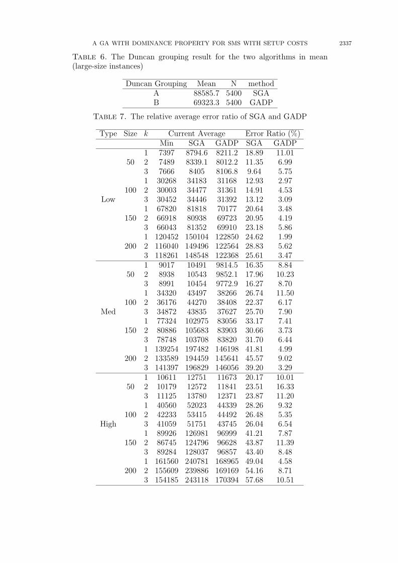
According to the results in Table 6, the average performance of GADP is better thanSGA and the differences are very obvious. Finally, Table 6 shows the result of Duncantest between the two algorithms and GADP is statistically better than SGA.

Finally, although it is not possible to obtain optimal solutions for large size of instancesin a limited time, this study ran the GADP for 1,000,000 solutions for each instance toderive a near-optimal solutions. Then, we ran SGA and GADP for 100,000 solutions toderive the current best objective value for each instance. The average relative error ratio((avgObj− currentMin)/currentMin) ∗ 100 is applied to distinguish the performance ofSGA and GADP. The result is shown in Table 7. We can find out that GADP outperformsthe other two methods for all different instances.

6. Discussions and Conclusions. This research studied the single machine schedulingproblem with sequence dependent setup times and the objective is to minimize the totaltardiness. This is a very important problem that is encountered in a wide variety of practi-cal situations. A set of dominance properties is developed in this research to determine therelationship between a pair of jobs. The time complexity of the dominance properties isin O(n2) and it is very efficient when combined with the GA. To speed up the convergenceof GA, these dominance properties are further integrated with a genetic algorithm whichis named GADP in short. From the experimental results, these dominance properties areable to generate a set of very good initial solutions and the GA procedures can furtherevolve these solutions into near-optimal solutions. The solution quality of GADP is muchbetter than that of a simple GA. It can be concluded that these dominance properties arevery effective in generating good quality of initial solutions. Therefore, GADP is moreefficient and effective when compared with a simple GA. For a set of large instances suchas 150, 200 or even larger job sizes, GADP still performs the best among others.


Table 5. The experimental results for the three different algorithms (par-tial large-size instance)

Type Size k SGA Obj Value GADP Obj ValueMin Mean Max Min Mean Max

1 8229 8794.6 9424 7397 8211.2 876750 2 7753 8339.1 8850 7489 8012.2 8444

3 7750 8405 9037 7666 8106.8 85611 32914 34183 35711 30268 31168 32171

100 2 32665 34477 35942 30062 31361 32694Low 3 32776 34446 36296 30452 31392 32278

1 78688 81818 85833 67865 70177 71874150 2 76316 80938 83605 67999 69723 71263

3 79011 81352 85989 68478 69910 720011 145254 150104 154839 120452 122850 125300

200 2 143730 149496 154344 119157 122564 1246253 142487 148548 157893 120217 122368 1250741 9391 10491 11957 9017 9814.5 10399

50 2 9308 10543 11504 8938 9852.1 105583 9157 10454 11873 8991 9772.9 107411 41240 43497 46031 35844 38266 40717

100 2 41955 44270 47300 36176 38408 40083Med 3 41874 43835 48138 34872 37627 39840

1 97679 102975 111951 79865 83056 85680150 2 99005 105683 113085 80886 83903 86699

3 97373 103708 110166 81139 83820 867361 184194 197482 204554 141130 146198 150477

200 2 182665 194459 200625 142235 145641 1486783 186634 196829 206540 142708 146056 1511771 11577 12751 14026 10611 11673 12849

50 2 11289 12572 13540 10179 11841 138863 12178 13780 15899 11125 12371 137031 48572 52023 56383 41878 44339 47249

100 2 48016 53415 57755 42233 44492 47300High 3 47989 51751 55985 41059 43745 46483

1 117097 126981 134396 91331 96999 102956150 2 119629 124796 129865 91850 96628 101090

3 121124 128037 135771 89284 96857 1017711 227667 240781 254946 162533 168965 175379

200 2 223495 239886 260765 162936 169169 1773663 228726 243118 270010 161974 170394 177203


Table 6. The Duncan grouping result for the two algorithms in mean(large-size instances)

Duncan Grouping Mean N methodA 88585.7 5400 SGAB 69323.3 5400 GADP

Table 7. The relative average error ratio of SGA and GADP

Type Size k Current Average Error Ratio (%)Min SGA GADP SGA GADP

1 7397 8794.6 8211.2 18.89 11.0150 2 7489 8339.1 8012.2 11.35 6.99

3 7666 8405 8106.8 9.64 5.751 30268 34183 31168 12.93 2.97

100 2 30003 34477 31361 14.91 4.53Low 3 30452 34446 31392 13.12 3.09

1 67820 81818 70177 20.64 3.48150 2 66918 80938 69723 20.95 4.19

3 66043 81352 69910 23.18 5.861 120452 150104 122850 24.62 1.99

200 2 116040 149496 122564 28.83 5.623 118261 148548 122368 25.61 3.471 9017 10491 9814.5 16.35 8.84

50 2 8938 10543 9852.1 17.96 10.233 8991 10454 9772.9 16.27 8.701 34320 43497 38266 26.74 11.50

100 2 36176 44270 38408 22.37 6.17Med 3 34872 43835 37627 25.70 7.90

1 77324 102975 83056 33.17 7.41150 2 80886 105683 83903 30.66 3.73

3 78748 103708 83820 31.70 6.441 139254 197482 146198 41.81 4.99

200 2 133589 194459 145641 45.57 9.023 141397 196829 146056 39.20 3.291 10611 12751 11673 20.17 10.01

50 2 10179 12572 11841 23.51 16.333 11125 13780 12371 23.87 11.201 40560 52023 44339 28.26 9.32

100 2 42233 53415 44492 26.48 5.35High 3 41059 51751 43745 26.04 6.54

1 89926 126981 96999 41.21 7.87150 2 86745 124796 96628 43.87 11.39

3 89284 128037 96857 43.40 8.481 161560 240781 168965 49.04 4.58

200 2 155609 239886 169169 54.16 8.713 154185 243118 170394 57.68 10.51


REFERENCES

[1] B. Alidaee and I. Dragan, A note on minimizing the weighted sum of tardy and early completionpenalties in a single machine: A case of small common due date, European Journal of OperationalResearch, vol.96, no.3, pp.559-563, 1997.

[2] M. H. Al-Haboubi and S. Z. Selim, A sequencing problem in the weaving industry, European Journalof Operational Research, vol.66, no.1, pp.65-71, 1993.

[3] A. Allahverdi, J. N. D. Gupta and T. Aldowaisan, A review of scheduling research involving setupconsideration, OMEGA, vol.27, no.2, pp.219-239, 1999.

[4] M. Azizoglu and S. Webster, Scheduling job families about an unrestricted common due date on asingle machine, International Journal of Production Research, vol.35, no.5, pp.1321-1330, 1997.

[5] U. Bagchi, R. Sullivan and Y.-L. Chang, Minimizing mean absolute deviation of completion timesabout a common due date, Naval Research Logistics Quarterly, vol.33, no.2, pp.227-240, 1986.

[6] K. R. Baker and G. D. Scudder, Sequencing with earliness and tardiness penalties: A review, Oper-ations Research, vol.38, no.1, pp.22-36, 1990.

[7] P. C. Chang, J. C. Hsieh and Y. W. Wang, Genetic algorithms applied in BOPP film schedulingproblems, Applied Soft Computing, vol.3, no.2, pp.139-148, 2003.

[8] P. C. Chang, J. C. Hsieh and Y. W. Wang, Adaptive multi-objective genetic algorithms for schedulingof drilling operation in printed circuit board industry, Applied Soft Computing, vol.7, no.3, pp.800-806, 2007.

[9] P. C. Chang, S. H. Chen and K. L. Lin, Two phase sub-population genetic algorithm for parallelmachine scheduling problem, Expert Systems with Applications, vol.29, no.3, pp.705-712, 2005.

[10] P. C. Chang, J. C. Hsieh and C. H. Liu, A case-injected genetic algorithm for single machine sched-uling problems with release time, International Journal of Production Economics, vol.103, no.2,pp.551-564, 2006.

[11] P. C. Chang, H. S. Chen and V. Mani, Parametric analysis of bi-criterion single machine schedulingwith a learning effect, International Journal of Innovational Computing, Information and Control,vol.4, no.8, pp.2033-2043, 2008.

[12] S.-H. Chen, P.-C. Chang, Q. Zhang and C.-B. Wang, A guided memetic algorithm with probabilisticmodels, International Journal of Innovational Computing, Information and Control, vol.5, no.12(B),pp.4753-4764, 2009.

[13] Z.-L. Chen, Scheduling with batch setup times and earliness-tardiness penalties, European Journalof Operational Research, vol.96, no.3, pp.518-537, 1997.

[14] T. C. E. Cheng, Optimal single-machine sequencing and assignment of common due-dates, Computersand Industrial Engineering, vol.22, no.2, pp.115-120, 1992.

[15] B. J. Coleman, A simple model for optimizing the single machine early/tardy problem with sequence-dependent setups, Production and Operation Management, vol.1, no.2, pp.225-228, 1992.

[16] S. French, Sequencing and Scheduling: An Introduction to the Mathematics of the Job-Shop, Wiley,New York, 1982.

[17] V. Gordon, J. Proth and C. Chu, A survey of the state-of-the-art of common due date assignmentand scheduling research, European Journal of Operational Research, vol.139, no.1, pp.1-25, 2002.

[18] N. G. Hall, W. Kubiak and S. P. Sethi, Earliness-tardiness scheduling problems, II: Deviation ofcompletion times about a restrictive common due date, Operations Research, vol.39, no.5, pp.847-856, 1991.

[19] N. G. Hall and S. M. E. Posner, Earliness-tardiness scheduling problems, I: Weighted deviation ofcompletion times about a common due date, Operations Research, vol.39, no.5, pp.836-846, 1991.

[20] Y. Hirashima, A Q-learning system for container transfer scheduling based on shipping order atcontainer terminals, International Journal of Innovative Computing, Information and Control, vol.4,no.3, pp.547-558, 2008.

[21] X. Hu, M. Huang and A. Z. Zeng, An intelligent solution system for a vehicle routing problem inurban distribution, International Journal of Innovative Computing, Information and Control, vol.3,no.1, pp.189-198, 2007.

[22] F. Jin, J. N. D. Gupta, S. Song and C. Wu, Single machine scheduling with sequence-dependentfamily setups to minimize maximum lateness, Journal of the Operational Research Society, 2009.

[23] J. J. Kanet, Minimizing the average deviation of job completion times about a common due date,Naval Research Logistics, vol.28, no.4, pp.643-651, 1981.

[24] O. I. Kulak and O. Yilmaz, PCB assembly scheduling for collect-and-place machines using geneticalgorithms, International Journal of Production Research, vol.45, no.17, pp.3949-3969, 2007.


[25] J. K. Lenstra, A. H. G. Rinnooy Kan and P. Brucker, Complexity of machine scheduling problems,Annals of Discrete Mathematics, vol.1, pp.343-362, 1977.

[26] T. Ma, Q. Yan, D. Guan and S. Lee, Research on task scheduling algorithm in grid environment,ICIC Express Letters, vol.4, no.1, pp.1-6, 2010.

[27] S. A. Mondal and A. K. Sen, Single machine weighted earliness-tardiness penalty problem with acommon due date, Computers & Operation Research, vol.28, no.7, pp.649-669, 2001.

[28] P. S. Ow and E. T. Morton, The single machine early/tardy problem, Management Science, vol.35,no.2, pp.177-191, 1989.

[29] G. Rabadi, M. Mollaghasemi and G. C. Anagnostopoulos, A branch-and-bound algorithm for theearly/tardy machine scheduling problem with a common due-date and sequence-dependent setuptime, Computers & Operation Research, vol.31, no.10, pp.1727-1751, 2001.

[30] F. Sourd, Earliness-tardiness scheduling with setup considerations, Computers & Operations Re-search, vol.32, no.7, pp.1849-1865, 2005.

[31] L. H. Su and P. C. Chang, A heuristic to minimize a quadratic function of job lateness on a singlemachine, International Journal of Production Economics, vol.55, no.2, pp.169-175, 1998.

[32] L. H. Su and P. C. Chang, Scheduling n jobs on one machine to minimize the maximum lateness witha minimum number of tardy jobs, Computers and Industrial Engineering, vol.40, no.4, pp.349-360,2001.

[33] J.-J. Wang, F. Liu and P. He, Rescheduling under predictive disruption of WSPT schedule for singlemachine scheduling, ICIC Express Letters, vol.4, no.2, pp.467-472, 2010.

[34] S. D. Wu, R. H. Storer and P. C. Chang, One machine rescheduling heuristic with efficiency andstability as criteria, Computers & Operations Research, vol.20, no.1, pp.1-14, 1993.

Appendix 1. The detail proofs of dominance properties.The following is the detail proofs of the dominance properties in Section 3.

1.1 Dominance properties of adjacent interchange.


X , for any two adjacent jobs (job i and job j) areearly and on-time, then the total deviation of Z(


∏X) only when



Proof: Figure 4 shows this condition and the objective of Z(∏

X) and Z(∏

Y ).

∵ G1 =b−2∑k=1

(k − 1)AP[k−1][k]

G2 = (i− 1)AP[i−1][i] + (j − 1)AP[i][j]

G3 = (n− j)AP[j][j+1] +n−1∑

k=b+1

(n− k)AP[k][k+1]

G′

1 = G1

G′

2 = (i− 1)AP[i−1][j] + (j − 1)AP[j][i]

G′

3 = (n− j)

(AP[i][i+1] +

n−1∑k=b+1

AP[k][k+1]

)Let X = Z(

∏Y )−Z(

∏X) and if X < 0, it means

∏Y is better than

∏X which satisfies



So job i and job j are interchanged.



X , for any two adjacent jobs (job i and job j) areon-time and tardy, then the total deviation of Z(


∏X) only when




X) and Z(∏

Y ).

∵ G1 =b−1∑k=1

(k − 1)AP[k−1][k]

G2 = (n− i)AP[i][j] + (i− 1)AP[i−1][i]

G3 = (n− j)AP[j][j+1] +n−1∑

k=b+2

(n− k)AP [k][k+1]

G′

1 = G1

G′

2 = (n− i)AP[j][i] + (i− 1)AP[i−1][j]

G′

3 = (n− j)AP[i][j+1] +n−1∑

k=b+2

(n− k)AP[k][k+1]

Let X = Z(∏

Y )− Z(∏






X , for any two adjacent jobs (job i and job j) aretardy and tardy, then the total deviation of Z(


∏X) only when




X) and Z(∏

Y ).

∵ G1 =b∑

k=1

(k − 1)AP[k−1][k] +i−1∑k=b

(n− k)AP[k][k+1]

G2 = (n− i+ 1)AP[i−1][i] + (n− j + 1)AP[i][j]

G3 = (n− j)AP [j][j+1]

n−1∑k=j

(n− k)AP[k][k+1]

G′

1 = G1

G′

2 = (n− i+ 1)AP[i−1][j] + (n− j + 1)AP[j][i]

G′

3 = (n− j)AP[i][j+1] +n−1∑

k=j+1

(n− k)AP[k][k+1]

Let X = Z(∏

Y )− Z(∏






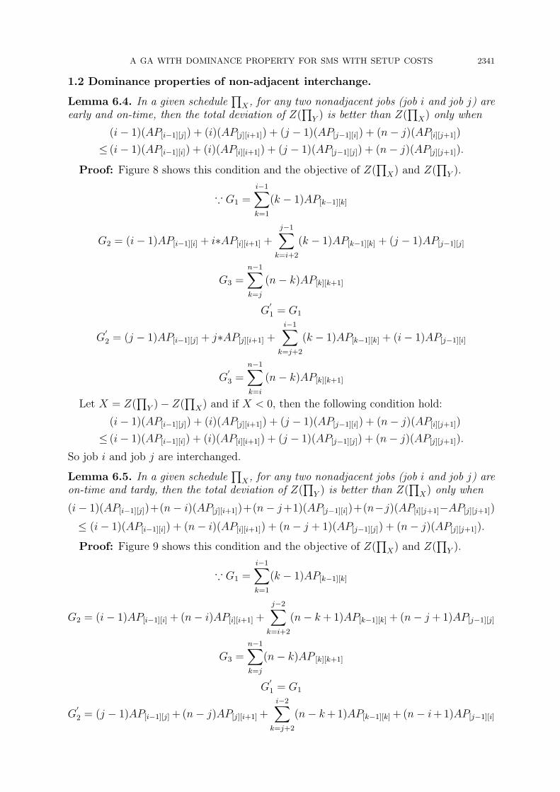
1.2 Dominance properties of non-adjacent interchange.


X , for any two nonadjacent jobs (job i and job j) areearly and on-time, then the total deviation of Z(


∏X) only when




X) and Z(∏

Y ).

∵ G1 =i−1∑k=1

(k − 1)AP[k−1][k]

G2 = (i− 1)AP[i−1][i] + i∗AP[i][i+1] +

j−1∑k=i+2

(k − 1)AP[k−1][k] + (j − 1)AP[j−1][j]

G3 =n−1∑k=j

(n− k)AP[k][k+1]

G′

1 = G1

G′

2 = (j − 1)AP[i−1][j] + j∗AP[j][i+1] +i−1∑

k=j+2

(k − 1)AP[k−1][k] + (i− 1)AP[j−1][i]

G′

3 =n−1∑k=i

(n− k)AP[k][k+1]

Let X = Z(∏

Y )− Z(∏






X , for any two nonadjacent jobs (job i and job j) areon-time and tardy, then the total deviation of Z(


∏X) only when

(i− 1)(AP[i−1][j])+(n− i)(AP[j][i+1])+(n− j+1)(AP[j−1][i])+(n−j)(AP[i][j+1]−AP[j][j+1])



X) and Z(∏

Y ).

∵ G1 =i−1∑k=1

(k − 1)AP[k−1][k]

G2 = (i− 1)AP[i−1][i] + (n− i)AP[i][i+1] +

j−2∑k=i+2

(n− k+ 1)AP[k−1][k] + (n− j + 1)AP[j−1][j]

G3 =n−1∑k=j

(n− k)AP [k][k+1]

G′

1 = G1

G′

2 = (j − 1)AP[i−1][j]+(n− j)AP[j][i+1]+i−2∑

k=j+2

(n− k+1)AP[k−1][k]+(n− i+1)AP[j−1][i]


G′

3 =n−1∑k=i

(n− k)AP [k][k+1]

Let X = Z(∏

Y )− Z(∏


(i− 1)(AP[i−1][j])+(n− i)(AP[j][i+1])+(n− j+1)(AP[j−1][i])+(n−j)(AP[i][j+1]−AP[j][j+1])




X , for any two nonadjacent jobs (job i and job j) areboth tardy, then the total deviation of Z(


∏X) only when




X) and Z(∏

Y ).

∵ G1 =b∑

k=1

(k − 1)AP[k−1][k] +i−1∑k=b

(n− k)AP[k][k+1]

G2 = (n− i+1)AP[i−1][i]+(n− i)AP[i][i+1]+

j−1∑k=i+2

(n− k+1)AP[k−1][k]+(n− j+1)AP[j−1][j]

G3 =n−1∑k=j

(n− k)AP[k][k+1]

G′

1 = G1

G′

2 = (n− j+1)AP[i−1][j]+(n− j)AP[j][i+1]+

j−1∑k=j+2

(n− k+1)AP[k−1][k]+(n− i+1)AP[j−1][i]

G′

3 =n−1∑k=i

(n− k)AP[k][k+1]

Let X = Z(∏

Y )−Z(∏

X) and if X < 0, it means∏

Y is better than∏

X which satisfies



So job i and job j are swapped.


X , for any two jobs (job i and job j) are early andtardy, then the total deviation of Z(


∏X) only when

(i− 1)(AP[i−1][j]) + (i)(AP[j][i+1]) + (n− j + 1)(AP[j−1][i]) + (n− j)(AP[i][j+1])

≤ (i− 1)(AP[i−1][i]) + (i)(AP[i][i+1]) + (n− j + 1)(AP[j−1][j]) + (n− j)(AP[j][j+1]).


X) and Z(∏

Y ).

∵ G1 =i−1∑k=1

(k − 1)AP[k−1][k]


G2 =(i− 1)AP[i−1][i] + i∗AP[i][i+1] +b∑

k=i+2

(k − 1)AP[k−1][k]

+

j−1∑k=b

(n− k)AP[k][k+1] + (j − 1)AP[j−1][j]

G3 =n−1∑k=j

(n− k)AP[k][k+1]

G′

1 = G1

G′

2 =(j − 1)AP[i−1][j] + j∗AP[j][i+1] +b∑

k=j+2

(k − 1)AP[k−1][k]

+

j−1∑k=b

(n− k)AP[k][k+1] + (i− 1)AP[j−1][i]

G′

3 =n−1∑k=i

(n− k)AP[k][k+1]

Let X = Z(∏

Y )−Z(∏

X) and if X < 0, it means∏

Y is better than∏

X which satisfies

(i− 1)(AP[i−1][j]) + (i)(AP[j][i+1]) + (n− j + 1)(AP[j−1][i]) + (n− j)(AP[i][j+1])

≤ (i− 1)(AP[i−1][i]) + (i)(AP[i][i+1]) + (n− j + 1)(AP[j−1][j]) + (n− j)(AP[j][j+1]).

Therefore, job i and job j are exchanged.

A GENETIC ALGORITHM ENHANCED BY DOMINANCE … · A GENETIC ALGORITHM ENHANCED BY DOMINANCE...

Documents

Transcript of A GENETIC ALGORITHM ENHANCED BY DOMINANCE … · A GENETIC ALGORITHM ENHANCED BY DOMINANCE...