
A Generalized Convolution Model for Multivariate...
25
A Generalized Convolution Model for Multivariate Nonstationary Spatial Processes Anandamayee Majumdar † , Debashis Paul ‡ and Dianne Bautista * † Department of Mathematics and Statistics, Arizona State University, Tempe. Email : [email protected] ‡ Department of Statistics, University of California, Davis. Email : [email protected] * 1958 Neil Department of Statistics, Ohio State University, Columbus. Email : [email protected] Abstract We propose a flexible class of nonstationary stochastic models for multivariate spatial data. The method is based on convolutions of spatially varying covariance kernels and produces math- ematically valid covariance structures. This method generalizes the convolution approach sug- gested by Majumdar and Gelfand (2007) to extend multivariate spatial covariance functions to the nonstationary case. A Bayesian method for estimation of the parameters in the covariance model based on a Gibbs sampler is proposed, and applied to simulated data. Model comparison is performed with the coregionalization model of Wackernagel (2003) which uses a stationary bivariate model. Based on posterior prediction results, the performance of our model is seen to be considerably better. Key words: convolution, nonstationary process, posterior inference, predictive distribution, spa- tial statistics, spectral density. Running title : Generalized convolution model for spatial processes 1 Introduction Spatial modeling with flexible classes of covariance functions has become a central topic of spatial statistics in recent years. One of the traditional approaches to modeling spatial stochastic pro- cesses is to consider parametric families of stationary processes, or processes that can be described 1
Transcript of A Generalized Convolution Model for Multivariate...

A Generalized Convolution Model for Multivariate Nonstationary
Spatial Processes
Anandamayee Majumdar†, Debashis Paul‡ and Dianne Bautista∗
† Department of Mathematics and Statistics, Arizona State University, Tempe. Email :
‡ Department of Statistics, University of California, Davis. Email : [email protected]
∗ 1958 Neil Department of Statistics, Ohio State University, Columbus. Email : [email protected]
Abstract
We propose a flexible class of nonstationary stochastic models for multivariate spatial data.
The method is based on convolutions of spatially varying covariance kernels and produces math-
ematically valid covariance structures. This method generalizes the convolution approach sug-
gested by Majumdar and Gelfand (2007) to extend multivariate spatial covariance functions to
the nonstationary case. A Bayesian method for estimation of the parameters in the covariance
model based on a Gibbs sampler is proposed, and applied to simulated data. Model comparison
is performed with the coregionalization model of Wackernagel (2003) which uses a stationary
bivariate model. Based on posterior prediction results, the performance of our model is seen to
be considerably better.
Key words: convolution, nonstationary process, posterior inference, predictive distribution, spa-
tial statistics, spectral density.
Running title : Generalized convolution model for spatial processes
1 Introduction
Spatial modeling with flexible classes of covariance functions has become a central topic of spatial
statistics in recent years. One of the traditional approaches to modeling spatial stochastic pro-
cesses is to consider parametric families of stationary processes, or processes that can be described
1

through parametric classes of semi-variograms (Cressie, 1993). However, in spite of its simplic-
ity, computational tractability, and interpretability, stationarity assumption is often violated in
practice, particularly when the data come from large, heterogeneous, regions. In various fields
of applications, like soil science, environmental science, etc., it is often more reasonable to view
the data as realizations of processes that only in a small neighborhood of a location behave like
stationary processes. Also, it is often necessary to model two or more processes simultaneously and
account for the possible correlation among various coordinate processes. For example, Majumdar
and Gelfand (2007) consider an atmospheric pollution data consisting of 3 pollutants : CO, NO
and NO2, whose concentrations in the atmosphere are correlated. A key question studied in this
paper is modeling this correlation among the various coordinates while allowing for nonstationarity
in space for the multivariate process. We propose a flexible semiparametric model for multivariate
nonstationary spatial processes. First, we would like to give an overview of the existing literature
on nonstationary spatial modeling.
A considerable amount of literature over last decade or so focussed on modeling locally stationary
processes (Fuentes, 2002; Fuentes, Chen, Davis and Lackmann, 2005; Gelfand, Schmidt, Banerjee
and Sirmans, 2004; Higdon, 1997; Paciorek and Schervish, 2006; Nychka, Wikle and Royle, 2002).
Dahlhaus (1996, 1997) gives a more formal treatment of locally stationary processes in the time
series context in terms of evolutionary spectra of time series. The different approaches to mod-
eling the nonstationary processes described in these articles may be classified as semi-parametric
approaches to modeling covariance functions. Higdon (2002) and Higdon, Swall and Kern (1999)
model the process as a convolution of a stationary process with a kernel of varying bandwidth.
Thus, the observed process Y (s) is of the form Y (s) =∫
Ks(x)Z(x)dx, where Z(x) is a stationary
process, and the kernel Ks depends on the location s. Fuentes (2002) and Fuentes and Smith (2001)
consider a convolution model in which the kernel has a fixed bandwidth, while the process has a
2
spatially varying parameter. Thus,
Y (s) =∫
DK(s− x)Zθ(x)(s)dx, (1)
where {Zθ(x)(·) : x ∈ D} is a collection of independent stationary processes with covariance function
parameterized by the function θ(·). Nychka, Wikle and Royle (2002) consider a multiresolution
analysis-based approach to model the spatial inhomogeneity that utilizes the smoothness of the
process and its effect on the covariances of the basis coefficients, when the process is represented
in a suitable wavelet-type basis.
One of the central themes of the various modeling schemes described above is that a process
may be represented in the spectral domain locally as a superposition of Fourier frequencies with
suitable (possibly spatially varying) weight functions. Recent work of Pintore and Holmes (2006)
provides a solid mathematical foundation to this approach. Paciorek and Schervish (2006) derive an
explicit representation for the covariance function for Higdon’s model when the kernel is multivariate
Gaussian and use it to define a nonstationary version of the Matern covariance function by utilizing
the Gaussian scale mixture representation of positive definite functions. Also, there are works on
a different type of nonstationary modeling through spatial deformations (see e.g. Sampson and
Guttorp, 1992) which we shall not be concerned with in this paper.
The modeling approaches mentioned so far focus primarily on one dimensional processes. In this
paper, our main focus is on modeling nonstationary, multi-dimensional spatial processes. Existing
approaches to modeling the multivariate processes include the work by Gelfand et al. (2004) which
utilizes the idea of coregionalization that models the covariance of Y(s) (taking values in RN ) as
Cov(Y(s),Y(s′)) =N∑
j=1
ρj(s− s′)Tj ,
where ρj(·) are stationary covariance functions and Tj are positive semidefinite matrices of rank
1. Also, Chirstensen and Amemiya (2002) consider a different class of multivariate processes that
depend on a latent shifted-factor model structure.
3
The work presented in this paper can be viewed as a generalization of the convolution model
for correlated Gaussian processes proposed by Majumdar and Gelfand (2007). We extend the
aforementioned model to nonstationary settings. One key motivation is the assertion that when
spatial inhomogeneity in the process is well-understood in terms of dependence on geographical
locations, it makes sense to use that information directly in the specification of the covariance
kernel. For example, soil concentrations of Nitrogen, Carbon and other nutrients and/or pollu-
tants, which are spatially distributed, are relatively homogenous across similar land-use types (e.g.
agricultural, urban, desert, transportation - and so on), but are non-homogeneous across spatial
locations with different land-use types. Usually the land-use types and their boundaries are clearly
known (typically from satellite imagery). So this is an instance when nonstationary models are
clearly advantageous compared to stationary models. Another example is concerning land-values
and different economic indicators in a spatial area. Usually land-values are higher around (possibly
multiple) business centers, and such information may be incorporated in the model as the known
centers of the kernels described in (11). It is also important for modeling multidimensional pro-
cesses that the degree of correlations among the coordinate processes across different spatial scales
is allowed to vary. Keeping these goals in mind, we present a class of models that behave locally
like stationary processes, but are globally nonstationary. The main contributions of this paper are:
(i) specification of the multivariate spatial cross-covariance function in terms of Fourier transforms
of spatially varying spectra; (ii) incorporation of correlations among coordinate processes that vary
with both frequency and location; (iii) derivation of precise mathematical conditions under which
the process is nonsingular; and (iv) the provision for including local information about the process
(e.g. smoothness, scale of variability, gradient of spatial correlation along a given direction) directly
into the covariance model. The last goal is achieved by expressing the spatially varying coordi-
nate spectra fj(s, ω) (as in (7)) as a sum of kernel-weighted stationary spectra, where the kernels
have known shapes and different (possibly pre-specified) centers, bandwidths and orientations. We
also present a Bayesian estimation procedure based on Gibbs sampling for estimating a specific
4

parametric covariance function and study its performance through simulation studies.
The paper is organized as follows. We specify the model and discuss its properties in Section 2.
In Section 3, we propose a special parametric subclass that is computationally easier to deal with.
Also, we discuss various aspects of the model like parameter identifiability, and its relation to some
existing model, by focusing attention to a special bivariate model. In Section 4, we give an outline
of a simulation study to illustrate the characteristics of the various processes generated by our
model in the two-dimensional setting. In Section 5, we present a Bayesian estimation procedure
and conduct a simulation study to demonstrate its effectiveness. In Section 6, we discuss some
related research directions. Some technical details and a detailed outline of the Gibbs sampling
procedure for posterior inference are given in the supplementary material.
2 Construction of covariances through convolution
We consider a real-valued point-referenced univariate spatial process, Y (s), associated with loca-
tions s ∈ Rd. In this section, we construct a Gaussian spatial process model for an arbitrary finite
set of locations in a region D ⊂ Rd by generalizing the construction of Majumdar and Gelfand
(2007), and then extend it to whole of Rd.
2.1 Nonstationary covariance structure on a finite set in Rd
In this subsection, we aim to construct a class of nonstationary multivariate stochastic processes
on a finite set of points in Rd. Assume that the points {sl : l = 1, . . . , k} in Rd are given. Let
{Cjl : j = 1, . . . , N ; l = 1, . . . , k} be a set of stationary covariance kernels on Rd with corresponding
spectral density functions {fjl : j = 1, . . . , N ; l = 1, . . . , k} defined by
fjl(ω) =1
(2π)d
∫
Rd
e−iωT sCjl(s)ds, ω ∈ Rd.
Consider the Nk ×Nk matrix C, whose (j, j′)-th entry in the (l, l′)-th block, for 1 ≤ j, j′ ≤ N
5

and 1 ≤ l, l′ ≤ k, is denoted by cjl,j′l′ and is expressed as
cjl,j′l′ ≡ C?jj′(sl, sl′) =
∫
Rd
eiωT (sl−sl′ )fjl(ω)fj′l′(ω)ρjj′(ω)ρ0ll′(ω)dω, (2)
where ρjj′(·) are complex-valued functions satisfying ρjj′(ω) = ρj′j(ω), and ((ρ0ll′(ω)))k
l,l′=1 is a
nonnegative definite matrix, for every ω ∈ Rd. Thus, C? := ((C?jj′))
Nj,j′=1 is function from Rd × Rd
to RN×N . We require that max{maxj,j′ |ρjj′(ω)|, maxl,l′ |ρ0ll′(ω)|} ≤ 1 for all ω ∈ Rd.
We show that under appropriate conditions, the Nk×Nk matrix C = ((cjl,j′l′)) is a nonnegative
definite matrix. The (l, l′)-th block (of size N ×N) of the matrix C, for 1 ≤ l, l′ ≤ k, is
Cll′ =
C?11(sl, sl′) . . . C?
1N (sl, sl′)...
. . ....
C?N1(sl, sl′) . . . C?
NN (sl, sl′)
. (3)
For all ω ∈ Rd, define All′(ω), for 1 ≤ l, l′ ≤ k, as
All′(ω) = eiωT (sl−sl′ )ρ0ll′(ω)
(f1l(ω))2ρ11(ω) . . . f1l(ω)fNl(ω)ρ1N (ω)...
. . ....
fNl(ω)f1l(ω)ρN1(ω) . . . (fNl(ω))2ρNN (ω)
(4)
where the fjl(ω)’s are as defined above. Let e(ω) be the k×k matrix with (l, l′)-th entry eiωT (sl−sl′ ),
1 ≤ l, l′ ≤ k, R(ω) = ((ρjj′(ω)))Njj′=1, and R0(ω) = ((ρ0
ll′(ω)))kll′=1. Let
F(ω) = diag(f11(ω), . . . , fN1(ω), . . . , f1k(ω), . . . , fNk(ω)),
and define A(ω) to be the Nk × Nk matrix with (l, l′)-th block All′(ω), for 1 ≤ l, l′ ≤ k. Then
A(ω) = F(ω)[(e(ω) ¯ R0(ω)) ⊗ R(ω)]F(ω), where ¯ denotes Schur (or Hadamard) product, i.e.,
coordinate-wise product of two matrices of same dimension, and ⊗ denotes the Kronecker product.
Note that, for an arbitrary a ∈ Ck, a∗(e(ω) ¯ R0(ω))a = b∗R0(ω)b, where bl = ale−iωT sl ,
l = 1, . . . , k. Therefore, if R0(ω) is positive definite, then so is the k × k matrix e(ω) ¯ R0(ω).
Since, F(ω) is diagonal with nonnegative diagonal entries, from (4), wherever F(ω) is p.d., A(ω) is
6

p.d. (n.n.d.) if both R(ω) and R0(ω) are p.d. (at least one n.n.d. but not p.d.). From (2),
C =∫
Rd
A(ω)dω (5)
where the integral is taken over every element of the matrix A(ω). By Cauchy-Schwarz inequality
and the fact that max{|ρjj′(ω)|, |ρ0ll′(ω)|} ≤ 1, a sufficient condition for the integrals in (5) to be
finite is that max1≤j≤N max1≤l≤k
∫(fjl(ω))2dω < ∞. Therefore we obtain the results:
Lemma 1 Sufficient conditions for C to be positive definite are that (i) the Nk×Nk matrix A(ω)
is nonnegative definite, and is positive definite on a set of positive Lebesgue measure in Rd; and
(ii)∫Rd(fjl(ω))2dω < ∞ for all j = 1, . . . , N and l = 1, . . . , k.
Lemma 2 Suppose that there exists B ⊂ Rd with positive Lebesgue measure such that for all ω ∈ B,
we have fjl(ω) > 0, for each j = 1, . . . , N , l = 1, . . . , k, and both R(ω) and R0(ω) := ((ρ0ll′(ω)))k
ll′=1
are positive definite matrices. Then A(ω) is a positive definite matrix on B.
As an immediate consequence of Lemmas 1 and 2 we have the following:
Theorem 1 Suppose that Cjl, 1 ≤ j ≤ N , 1 ≤ l ≤ k, are positive definite functions, and R(ω) =
((ρjj′(ω)))Nj,j′=1, and R0(ω) := ((ρ0
ll′(ω)))kll′=1 are nonnegative definite matrices for all ω ∈ Rd. If
there exists a set B ⊂ Rd with nonzero Lebesgue measure such that for all ω ∈ B, we have fjl(ω) > 0,
and∫Rd(fjl(ω))2dω < ∞, for each j and l, and both R(ω) and R0(ω) are positive definite on B, then
the matrix C as in (2) defines a valid cross-covariance structure of an N -dimensional stochastic
process on D = {s1, . . . , sk}.
In the above construction, since the Cjl’s, ρjj′ ’s and ρ0ll′ are arbitrary, a rich framework for
modeling spatial processes is achieved if we can generalize this from any arbitrary finite set {sl; l =
1, . . . , k} to an arbitrary spatial region D ∈ Rd. Next corollary states that this holds in the
stationary case (i.e., when fjl(ω) = fj(ω) for all l = 1, . . . , k, for all j, and ρ0ll′(ω) ≡ 1) if the matrix
R(ω) = ((ρjj′(ω)))Nj,j′=1 is nonnegative definite for all ω ∈ Rd.
7
Corollary 1 Suppose that C1, . . . , CN are valid covariance functions on Rd with spectral densities
f1, . . . , fN , respectively, and the functions ρjj′ are such that R(ω) := ((ρjj′(ω)))Njj′=1 is nonnegative
definite a.e. ω ∈ Rd. Then there is a mean-zero Gaussian stationary stochastic process Y(s) =
(Y1(s), . . . , YN (s)) on Rd such that
Cov(Yj(s), Yj′(t)) = C?jj′(s− t) :=
∫
Rd
eωT (s−t)fj(ω)fj′(ω)ρjj′(ω)dω. (6)
2.2 Construction of nonstationary covariances on Rd
We shall now generalize the construction of the nonstationary N ×N covariance function C? from
the set {s1, . . . , sk} to the entire space Rd. Since a Gaussian process is determined entirely by
its mean and covariance, given points s1, . . . , sk ∈ Rd, we can find a zero mean Gaussian random
vector (Yjl : 1 ≤ j ≤ N, 1 ≤ l ≤ k) with covariance matrix given by C?. Moreover, this vector
can be viewed as the realization of an N -dimensional random process Y(s) = (Y1(s), . . . , YN (s)) at
the points s1, . . . , sk, if we define Yjl = Yj(sl). The next theorem states that an extension of the
process Y(s) to arbitrary domains in Rd is possible.
Theorem 2 Let {fj(s, ω)}Nj=1, be non-negative functions on Rd×Rd, such that sups∈Rd
∫Rd(fj(s, ω))2dω <
∞. Let ρ0(s, s′, ω) be a valid correlation function on Rd × Rd for a.e. ω ∈ Rd. Also, let
R(ω) = ((ρjj′(ω)))Njj′=1 be nonnegative definite for every ω ∈ Rd. If there exist a set B ∈ Rd
with positive Lebesgue measure so that for every ω ∈ B, the function fj(·, ω) > 0, the matrix R(ω)
is positive definite, and the correlation function ρ0(·, ·, ω) is positive definite, then there exists an
N -dimensional Gaussian spatial process Y(s) on Rd with N × N -dimensional covariance kernel
C?(s, s′) whose entries are given by,
C?jj′(s, s
′) =∫
Rd
eiωT (s−s′)fj(s, ω)fj′(s′, ω)ρ0(s, s′, ω)ρjj′(ω)dω, s, s′ ∈ Rd. (7)
The function fj(s, ω) can be interpreted as a location-dependent spectral density of a locally
stationary stochastic process. If fj(s, ω) = fj(ω), for all j = 1, . . . , N , and ρ0(s, s′, ω) = 1, then C?
as in Theorem 2 becomes a covariance function of an N -dimensional stationary process on Rd.
8
2.3 Sufficient conditions for positive definiteness
In this subsection, we present a sufficient condition on the Fourier transforms of the cross-correlation
functions, namely {ρjj′}j 6=j′ , that guarantee the positive-definiteness of the covariance function in
the convolution model presented in Section 2.2, when the number of variables N is at most 4.
Theorem 3 When N ≤ 4, sufficient conditions for positive definiteness of R(ω) are :
(i) 1 > |ρjj′ |2 for all 1 ≤ j < j′ ≤ N .
(ii) 1 > |ρjl|2 + |ρlm|2 + |ρmj |2 − 2Re(ρjlρlmρmj), for all 1 ≤ j < l < m ≤ N .
(iii) If 1 ≤ j 6= l 6= m 6= n ≤ N , then
1− |ρlm|2 − |ρmn|2 − |ρnl|2 + 2Re(ρlmρmnρnl)
> |ρjl|2 + |ρjm|2 + |ρjn|2 − (|ρjl|2|ρmn|2 + |ρjm|2|ρln|2 + |ρjn|2|ρlm|2)
+2Re(ρjlρlmρmj) + 2Re(ρjmρmnρnj) + 2Re(ρjnρnlρlj)
−2Re(ρjlρlnρnmρmj)− 2Re(ρjmρmlρlnρnj)− 2Re(ρjnρnmρmlρlj).
Also, equality in place of any of the inequalities implies singularity of the matrix R(ω).
2.4 A general model
A general formulation for the nonstationary covariance kernels comes from introducing some struc-
ture to the correlation function ρ0(s, t, ω). One proposal is to consider
ρ0(s, t, ω) =∞∑
l=1
ρl(s, t)ψl(ω), (8)
where ρl are correlation functions on Rd × Rd, and ψl ≥ 0 are such that∑∞
l=1 ψl(ω) ≤ 1 a.e.
Recall that by spectral representation theory of stationary stochastic processes (Yaglom, 1962,
Schabenberger and Gotway, 2005), there exists an N -dimensional dimensional stochastic process
Z(ω) with independent coordinates, defined on Rd, such that the one dimensional stationary process
9

Xj(s) with covariance function given by Cjj(s− t) =∫Rd eiωT (s−t)(fj(ω))2dω, with
∫(fj(ω))2dω <
∞, can be represented as Xj(s) =∫Rd eiωT sfj(ω)dZj(ω). Pintore and Holmes (2006) consider
processes of the form
Xj(s) =∫
Rd
eiωT sfj(s, ω)dZj(ω),
where fj(s, ω) are of the form hj(s)fj(ω; θ(s)), where fj(·; θ) is the spectral density function of a
stationary stochastic process with parameter θ, and hj(·) is a nonnegative function, for each j =
1, . . . , N . These processes have covariance functions Cjj′(s, t) = δj−j′∫Rd eiωT (s−t)fj(s, ω)fj′(t, ω)dω
where δ0 = 1 and δk = 0 if k 6= 0. Our proposal can therefore be viewed as extending their method
to the multidimensional case while introducing spatially varying cross-correlation functions.
The setting described by (8) can be realized by describing the process Y(s) as
Y(s) =∞∑
l=1
ξl(s)∫
Rd
eiωT sF(s, ω) ·R1/2(ω)√
ψl(ω)dZ(ω), (9)
where R1/2(ω) is a nonnegative square-root of the matrix R(ω), and F(s, ω) is a diagonal matrix
with j-th diagonal element fj(s, ω). Here {ξl(s)}∞l=1 are uncorrelated (in the Gaussian case, indepen-
dent) stochastic processes, independent of the process Z(ω), with Cov(ξl(s), ξl(t)) = ρl(s, t). Ob-
serve that if the functions {ψl} are orthogonal, we have the formal expansion U(s, ω) =∑∞
l=1 ξl(s)ψl(ω),
defining a mean zero, L2 stochastic process on Rd × Rd with covariance function ρU (s, t, ω, ω′) =
Cov(U(s, ω), U(t, ω′)). Also, then ρ0(s, t, ω) = ρU (s, t, ω, ω). Then we can formally define,
Y(s) =∫
Rd
eiωT sU(s, ω)F(s, ω) ·R1/2(ω)dZ(ω), (10)
where the processes U(s, ω) are Z(ω) are assumed to be independent and defined on the same
probability space. Note that (10) is a formal integral representation, and we are assuming that all
the measurability conditions needed on the processes to define the stochastic integral are satisfied.
The most manageable case from a practical point of view though, in our opinion, is when ρl(s, t) =
ρ(s− t; θl) for some parametric correlation function ρ(·; θ).
10
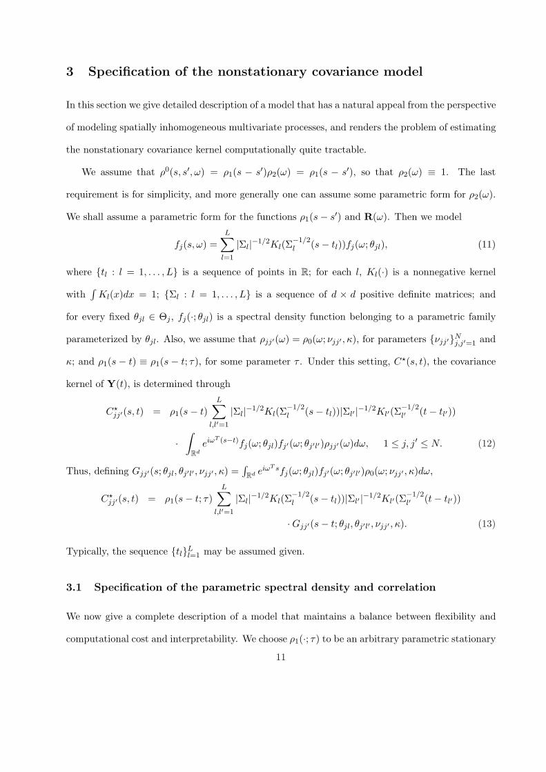
3 Specification of the nonstationary covariance model
In this section we give detailed description of a model that has a natural appeal from the perspective
of modeling spatially inhomogeneous multivariate processes, and renders the problem of estimating
the nonstationary covariance kernel computationally quite tractable.
We assume that ρ0(s, s′, ω) = ρ1(s − s′)ρ2(ω) = ρ1(s − s′), so that ρ2(ω) ≡ 1. The last
requirement is for simplicity, and more generally one can assume some parametric form for ρ2(ω).
We shall assume a parametric form for the functions ρ1(s− s′) and R(ω). Then we model
fj(s, ω) =L∑
l=1
|Σl|−1/2Kl(Σ−1/2l (s− tl))fj(ω; θjl), (11)
where {tl : l = 1, . . . , L} is a sequence of points in R; for each l, Kl(·) is a nonnegative kernel
with∫
Kl(x)dx = 1; {Σl : l = 1, . . . , L} is a sequence of d × d positive definite matrices; and
for every fixed θjl ∈ Θj , fj(·; θjl) is a spectral density function belonging to a parametric family
parameterized by θjl. Also, we assume that ρjj′(ω) = ρ0(ω; νjj′ , κ), for parameters {νjj′}Nj,j′=1 and
κ; and ρ1(s − t) ≡ ρ1(s − t; τ), for some parameter τ . Under this setting, C?(s, t), the covariance
kernel of Y(t), is determined through
C?jj′(s, t) = ρ1(s− t)
L∑
l,l′=1
|Σl|−1/2Kl(Σ−1/2l (s− tl))|Σl′ |−1/2Kl′(Σ
−1/2l′ (t− tl′))
·∫
Rd
eiωT (s−t)fj(ω; θjl)fj′(ω; θj′l′)ρjj′(ω)dω, 1 ≤ j, j′ ≤ N. (12)
Thus, defining Gjj′(s; θjl, θj′l′ , νjj′ , κ) =∫Rd eiωT sfj(ω; θjl)fj′(ω; θj′l′)ρ0(ω; νjj′ , κ)dω,
C?jj′(s, t) = ρ1(s− t; τ)
L∑
l,l′=1
|Σl|−1/2Kl(Σ−1/2l (s− tl))|Σl′ |−1/2Kl′(Σ
−1/2l′ (t− tl′))
·Gjj′(s− t; θjl, θj′l′ , νjj′ , κ). (13)
Typically, the sequence {tl}Ll=1 may be assumed given.
3.1 Specification of the parametric spectral density and correlation
We now give a complete description of a model that maintains a balance between flexibility and
computational cost and interpretability. We choose ρ1(·; τ) to be an arbitrary parametric stationary
11

correlation function on Rd, with parameter τ . We assume that fj(ω; θjl) is of the form cjlγ(ω; θjl)
for some scale parameter cjl > 0 (note that we express θjl = (cjl, θjl)), and a parametric class of
spectral densities γ(·; θ) that is closed under product. The latter means that given any m ≥ 1, there
exists a function γ(·; ·) and functions cγ(· · · ), dγ(· · · ) of m variables such that, given parameters
θ1, . . . , θm,m∏
i=1
γ(·; θi) = dγ(θ1, · · · , θm)γ(·; cγ(θ1, · · · , θm)).
In particular, γ(·; θ1) = dγ(θ1)γ(·; cγ(θ1)). For example, the spectral densities of the Matern family
(under some restrictions on the parameters), and the Gaussian family satisfy this property.
For j 6= j′, we express ρ0(ω; νjj′ , κ) as νjj′α(ω; κ), where α(ω; κ) ≡ α(ω) is a real-valued
function satisfying − 1N−1 ≤ α(ω) ≤ 1. We choose {νjj′}1≤j 6=j′≤N in such a way that the N × N
matrix N = ((νjj′))1≤j,j′≤N , with νjj ≡ 1 for all j, is positive definite (in fact, a correlation
matrix). Since the N ×N matrix A(ω) with diagonal elements 1, and off-diagonal elements α(ω)
is clearly positive definite (under the restriction α(ω) ∈ (− 1N−1 , 1]), the matrix R(ω) thus specified
is positive semidefinite for all ω, since the latter is just N¯A(ω). α(ω) = 1 for all ω corresponds
to the situation where the different coordinate processes have the same correlation structure at all
frequencies. To add flexibility to the model without making it computationally too cumbersome,
we propose the following structure for α(ω).
α(ω) =γ(ω; α1)γ(0; α1)
− βγ(ω;α2)γ(0;α2)
, (14)
where β ∈ [0, 1N−1) and α1, α2 are free parameters, and γ belongs to the same family of spectral
densities as the one used in specifying fj ’s. Thus κ = (α1, α2, β).
An obvious advantage of this restriction is that one has a closed form expression for Gjj′(s; θjl, θj′l′ , νjj′ , κ)
in terms of the inverse Fourier transform of the function γ : for 1 ≤ j 6= j′ ≤ N ,
Gjj′(s; θjl, θj′l′ , νjj′ , κ) = cjlcj′l′νjj′ ·[dγ(θjl, θj′l′ , α1)
γ(0;α1)(F−1γ)(s; cγ(θjl, θj′l′ , α1))
− βdγ(θjl, θj′l′ , α2)γ(0;α2)
(F−1γ)(s; cγ(θjl, θj′l′ , α2))
], (15)
12

where F−1γ denotes the inverse Fourier transform of γ, i.e. the covariance function whose spectral
density is γ. Also, for j = j′,
Gjj′(s; θjl, θj′l′ , νjj′ , κ) = cjlcjl′dγ(θjl, θjl′)(F−1γ)(s; cγ(θjl, θjl′)). (16)
3.2 A bivariate process
In many practical problems we are often interested in studying the joint behavior of two processes
at a time, e.g. soil salinity and soil moisture content; or, temperature and pressure fields etc. In
the bivariate case (N = 2), the general formulation for our model simplifies considerably. As stated
in Theorem 3, in order that(7) is a valid covariance kernel, it is sufficient that |ρ12(ω)|2 ≤ 1. Also,
the condition Im(ρ12(ω)) 6= 0 for ω ∈ B, for some B with positive Lebesgue measure, is necessary
to ensure that Cov(Y1(s), Y2(s′)) 6= Cov(Y2(s), Y1(s′)) (asymmetric cross-covariance). Our model
bridges the two extremes: ρ12(ω) ≡ 0 yields zero cross-correlation across all spatial locations, and
ρ12(ω) ≡ 1 specifies the singular cross-convolution model outlined in Majumdar and Gelfand (2007).
For the purpose of illustrating some of the main features of our model, we focus on a bivariate
non-stationary Gaussian process following the parametric covariance model presented in Section
3.1. We assume γ(·; θ) to be a Gaussian spectral density with scale parameter θ, so that γ(ω; θ) =
12(πθ)
− 12 e−ω2/4eθ. Hence, the parameters describing the product of m such densities with parameters
θ1, . . . , θm are
cγ(θ1, · · · , θm) =1∑m
i=1 1/θi
and dγ(θ1, · · · , θm) =1
2mπm/2
1∏m
i=1 θ1/2i
with γ(ω; θ) = e−ω2/4eθ. Moreover, in this case, we have (F−1γ)(s; θ) = e−eθ‖s‖2. Thus, the ex-
pression for Gjj′(s; θjl, θj′l′ , νjj′ , κ) can be simplified by noting that γ(0; θ) = dγ(θ) = 12(πθ)−1/2,
and (F−1γ)(s; θ) = 2(πθ)1/2e−eθ‖s‖2. Next, since the Cholesky decomposition of a positive definite
matrix can be chosen to be lower triangular, we express Σl− 1
2 as:
Σl− 1
2 =
σ11l 0
σ21l σ22l
(17)
13
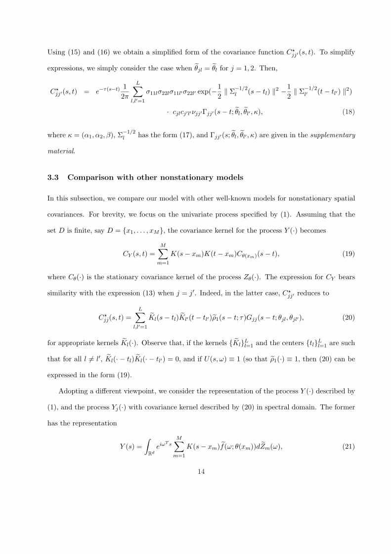
Using (15) and (16) we obtain a simplified form of the covariance function C?jj′(s, t). To simplify
expressions, we simply consider the case when θjl = θl for j = 1, 2. Then,
C?jj′(s, t) = e−τ(s−t) 1
2π
L∑
l,l′=1
σ11lσ22lσ11l′σ22l′ exp(−12‖ Σ−1/2
l (s− tl) ‖2 −12‖ Σ−1/2
l′ (t− tl′) ‖2)
· cjlcj′l′νjj′Γjj′(s− t; θl, θl′ , κ), (18)
where κ = (α1, α2, β), Σ−1/2l has the form (17), and Γjj′(s; θl, θl′ , κ) are given in the supplementary
material.
3.3 Comparison with other nonstationary models
In this subsection, we compare our model with other well-known models for nonstationary spatial
covariances. For brevity, we focus on the univariate process specified by (1). Assuming that the
set D is finite, say D = {x1, . . . , xM}, the covariance kernel for the process Y (·) becomes
CY (s, t) =M∑
m=1
K(s− xm)K(t− xm)Cθ(xm)(s− t), (19)
where Cθ(·) is the stationary covariance kernel of the process Zθ(·). The expression for CY bears
similarity with the expression (13) when j = j′. Indeed, in the latter case, C?jj′ reduces to
C?jj(s, t) =
L∑
l,l′=1
Kl(s− tl)Kl′(t− tl′)ρ1(s− t; τ)Gjj(s− t; θjl, θjl′), (20)
for appropriate kernels Kl(·). Observe that, if the kernels {Kl}Ll=1 and the centers {tl}L
l=1 are such
that for all l 6= l′, Kl(· − tl)Kl(· − tl′) = 0, and if U(s, ω) ≡ 1 (so that ρ1(·) ≡ 1, then (20) can be
expressed in the form (19).
Adopting a different viewpoint, we consider the representation of the process Y (·) described by
(1), and the process Yj(·) with covariance kernel described by (20) in spectral domain. The former
has the representation
Y (s) =∫
Rd
eiωT sM∑
m=1
K(s− xm)f(ω; θ(xm))dZm(ω), (21)
14
where Zm(·), m = 1, . . . , M are i.i.d. zero mean Brownian processes, and f(·; θ) is the spectral
density function of Cθ(·). Whereas, from (10) and (11), Yj(·) can be represented as
Yj(s) =∫
Rd
eiωT sU(s, ω)L∑
l=1
Kl(s− tl)fj(ω; θjl)dZj(ω), (22)
where Zj(·) is the j-th coordinate of Z(·). The two processes thus differ mainly by the fact that
(21) is a representation of Y (·) in terms of weighted sum of independent spectral processes {Zm(·)},
whereas Yj(·) is represented in terms of one spectral process Zj(·).
These comparisons also indicate that, as long as the kernels {Kl}Ll=1 and the centers {tl}L
l=1
are such that for all l 6= l′ the products Kl(· − tl)Kl(· − tl′) have comparatively small values,
the parameters in the model are identifiable. They can be identified essentially from the data on
different spatial locations. Indeed this will be the case if the centers {tl}Ll=1 are well-separated, and
the scale parameters Σl for the kernel Kl are comparatively small in magnitude. In practice, we
expect to have reasonable apriori information about the possible spatial inhomogeneity, so that
the specification of fairly accurate prior for the kernel centers {tl}Ll=1 is possible.
4 Simulation results
To understand the dependency of the model on various parameters, we perform a small simulation
study for the bivariate (N = 2) case, in which we specify L = 4; σ11l = 1, for all l = 1, . . . , 4; β = 0.5,
ν12 = ν21 = 0.5, α2 = 0.2, τ = 0.5. We generate 100 realizations (on the unit square [0, 1]×[0, 1]) of a
bivariate spatial process with centers of the four kernels t1 = (0.1, 0.7), t2 = (0.6, 0.1), t3 = (0.9, 0.6),
t4 = (0.6, 0.9). Changing the values of σ21l, σ22l, cjl, θjl and α1, we generate data from 8 different
models as given in Table 1. If we generalize this to N(≥ 2) processes and L kernels, then the
number of parameters becomes [N(N + 1)/2 + 3N ]L + N(N − 1)/2 + 4. Note that the first term
within bracket N(N + 1)/2 corresponds to Σl; the second term within brackets corresponds to
{cjl}Nj=1, {θjl}N
j=1 and tl; and the term N(N − 1)/2 corresponds to {νjj′}1≤j<j′≤N .
Qualitative features of the nonstationarity are illustrated through the contour plot of V ar(Y (s))
15

σ11l= 1 θjl = (cjl, eθjl) α2 = 0.2
Model σ21l σ22l cjleθjl α1
(1) 3.0 3 2p
j/lp
1/l 0.1
(2) 8.0 3 2p
j/lp
1/l 0.1
(3) 3.0 3 10jlp
1/l 0.1
(4) 8.0 3 10jlp
1/l 0.1
(5) 3.0 5 2p
j/lp
1/l 0.1
(6) 8.0 5 2p
j/lp
1/l 0.1
(7) 3.0 3 2p
j/lp
1/l 0.4
(8) 8.0 3 2p
j/l j + l 0.1
Table 1: Parameter specification of the 8 different models.
against s (Figure 1). A sample realization of each process is plotted in Figure 4 (in the supplemen-
tary material). From the figures, we clearly note distinct patterns variations among the variance
profiles as well as sample realizations of the 8 processes. Thus, all the parameters seem to have
considerable effects on the processes, and with the flexibility of these local and global parameters,
we can generate a wide class of non-stationary multivariate spatial models.
5 Bayesian modeling and inference
We first give an outline of a Bayesian approach for estimating the parameters of the general N -
dimensional model specified in Section 3.1. We assume an exponential correlation structure (Stein,
1999) for ρ1(·, τ), and a Gaussian spectral density for γ(·; θ), where τ > 0 is a global decay parame-
ter. We assign a Gamma(aτ , bτ ) prior for τ , with aτ , bτ > 0. We set apriori cjliid∼ Gamma(acjl
, bcjl),
and θjliid∼ Gamma(aeθjl
, beθjl). We specify i.i.d. InvWishart(Ψ, 2) priors for Σl, with mean matrix
Ψ. The choice of scale parameter is to allow larger variability. In order to specify a prior for the
parameters {νjj′}, we consider an N ×N positive definite matrix ν?, and define
N := ((νjj′))Nj,j′=1 = diag(ν?)−
12 ν?diag(ν?)−
12 .
We set apriori ν? ∼ InvWishart(ν, d) where ν is an N × N positive definite correlation matrix
(to avoid over-parametrization), whose structure represents our prior belief about the strength and
directionality of association of the different coordinate processes. In geophysical context this may
16

mean knowledge about the states of the physical process. Note that this ensures the positive-
definiteness of the matrix N, and additionally sets the diagonals νjj = 1, as required. When
N = 2, there is only one unknown parameter in this matrix N, viz. ν12. And so, we may specify
the prior ν12 ∼ Unif(−1, 1) which guarantees that N is p.d. Since the permissible range of β is
[0, 1N−1 ], we assume the prior of β to be β ∼ Unif(0, 1
N−1). We assume independent Gamma
priors Gamma(aαk, bαk
), k = 1, 2, for the positive parameters α1, α2, respectively.
5.1 Results in a special bivariate case
We now discuss some simulation results for the special case of the bivariate model specified in
Section 3.2. We fix σ11l = σ11, σ22l = σ22, σ21l = σ21, cjl = c and θjl = θ for all l = 1, . . . , L; and
α1 = α2 = α. Since β and ν12 are not identifiable together, we set β = 0 in the model. This non-
identifiability arises when α1 = α2 = α, but not when α1 6= α2. Further, we choose σ11 = σ22 = 1,
τ = 0.1, c = 2, θ = 0.1, α = 0.1, σ21 = 1 and ν21 = 0.8. We generate bivariate Gaussian data with
mean 0. For estimation, we treat β, σ11, σ22 and τ as known, and the other five parameters as
unknown and estimate them from the data using the Gibbs sampling procedure.
From equations (18), (23) and (24), it transpires that c2 is a scale parameter, and we employ
an InvGamma(2, 1) prior for c2, i.e., E(c2) = 1 and V ar(c2) = ∞. For the (positive) parameter
α, we assume Gamma(0.01, 10) prior, so that E(α) = 0.1 and V ar(α) = 1. For θ, we assume
Gamma(0.1, 10) prior, so that E(θ) = 1 and V ar(θ) = 10. Since ν21 is restricted to the interval
(−1, 1), and is a measure of global association between processes, we assume a positive association,
and choose a Uniform(0, 1) prior. Finally, we choose a N(0, 10) prior for σ21.
The posterior distribution of c2 is an Inverse Gamma. The posterior distributions of rest of
the parameters do not have closed form. Hence we employ Gibbs sampling within a Metropolis
Hastings algorithm to obtain posterior samples of the parameters. Burn-in was obtained with 2000
iterations and we thinned the samples by 20 iterations to obtain 1000 uncorrelated samples from
the joint posterior distribution of (c, θ, α, σ21, ν21) given the data. Sensitivity analysis of the priors
17
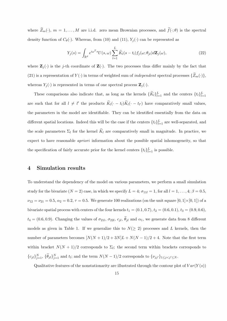
Parameter value Posterior values n = 15 n = 25 n = 50
Mean, s.d. 2.13, 0.43 1.96, 0.45 2.08, 0.49
c = 2 Median 2.07 1.91 2.08
95% credible interval (1.32, 3.12) (1.21, 2.89) (1.12, 3.05)
Mean, s.d. 0.54, 0.28 0.59, 0.27 0.69, 0.21
ν21 = 0.8 Median 0.54 0.65 0.72
95% credible interval (0.03, 0.98) (0.10, 0.98) (0.22, 0.98)
Mean, s.d. 0.93, 0.40 0.85, 0.37 1.27,0.36
σ21 = 1 Median 0.96 0.87 1.27
95% credible interval (0.03, 1.66) (0.06, 1.54) (0.50, 1.92)
Mean, s.d. 0.10, 0.10 0.12, 0.10 0.12, 0.10
α = 0.1 Median 0.07 0.09 0.09
95% credible interval (0.003, 0.37) (0.005, 0.30) (0.007, 0.35)
Mean, s.d. 0.30, 0.25 0.27, 0.33 0.13, 0.11
θ = 0.1 Median 0.24 0.15 0.10
95% credible interval: (0.02, 0.97) (0.02, 1.18) (0.01, 0.42)
Table 2: Posterior mean, standard deviation, median and 95% credible intervals of parameters
has been carried out by varying the means and variances. The priors prove to be fairly robust with
respect to the posterior inference results. For data simulated using n = 15, 25 and 50 locations, we
present the results of the posterior inference in Table 2. This table displays the posterior mean,
standard deviation (s.d.), median and 95% credible intervals of each of the five parameters treated
as random in the model. Table 2 shows that for each n, the 95% credible intervals contain the
actual values of the parameters. The lengths of the intervals for ν21 and α are relatively large.
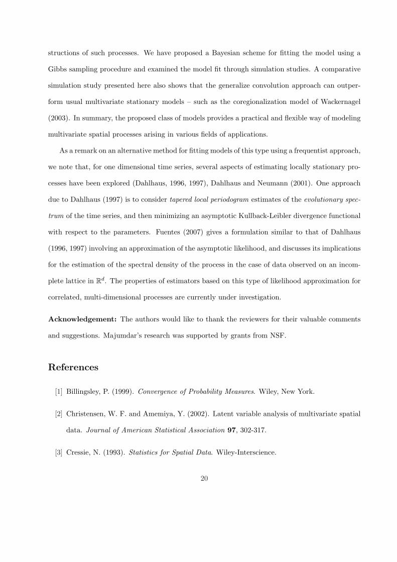
In order to gain further insight about the performance as sample size increases, we carry out a
separate simulation study: we simulate 100 samples independent samples of sizes n = 15, 25 and
50, respectively, from the bivariate model for the specified values of the parameters, and run the
MCMC each time on each of these samples. Boxplots of the mean and median of the posterior
squared errors (SE) of the covariance terms at three different spatial locations for the three sample
sizes are displayed in Figure 2. The reported values are generically of the form Mean/Median
(SE(Cov(Yk(si), Yk′(si′)))/{Cov(Yk(si), Yk′(si′))}2), i.e, they represent the mean and the median
of the standardized forms of the posterior SE From Figure 2, we observe that the means and
medians of the posterior standardized SE are rather small, and these values decrease with larger
18

sample sizes, as is to be expected.
Further, to compare the prediction performance of our model with that of a known bivariate
stationary spatial model, we use the coregionalization model (stationary) of Wackernagel (2003)
as implemented by the spBayes package (Finley, Banerjee and Carlin, 2007) in R, and compare
predictive distributions of terms such as (θpred − θ)2 where θ is the variance or covariance of the
data generated using the true model (i.e, the generalized convolution model) at specific locations,
and θpred are the posterior predictive sample estimates of θ. We compare the two fitted models for
n = 25 and n = 50, using medians of (θpred − θ)2/θ2 for standardizing the results. The spBayes
package uses priors with large variances (infinite variance for scale or variance parameters) for
all but one of the parameters used in the model, and that is also the case in our model. One
parameter, namely the decay parameter, has been assigned a mean of 0.18 and variance of 0.54
in the model implemented by spbayes. The generalized convolution model on the other hand,
assigns a prior to the parameter α with mean 0.1 and variance 1. No hyper-prior is used in either
model. Figure 3 clearly shows the stark contrast in performance of the stationary coregionalization
versus nonstationary generalized convolution model. For our model, median of posterior predictive
squared errors are close to 0 for all values, whereas many of the values of this performance measure
corresponding to the stationary model are extremely large. This seems to indicate that for cases
where nonstationarity prevails in the underlying multivariate spatial processes, our model is a
better choice than the regular coregionalization model of Wackernagel (2003), as implemented by
the spBayes package.
6 Discussion and concluding remarks
We have proposed a flexible class of spatially varying covariance and cross-covariance models for
univariate and multivariate nonstationary Gaussian spatio-temporal processes, with practical ways
of incorporating information about inhomogeneity, and discussed some possible mathematical con-
19
structions of such processes. We have proposed a Bayesian scheme for fitting the model using a
Gibbs sampling procedure and examined the model fit through simulation studies. A comparative
simulation study presented here also shows that the generalize convolution approach can outper-
form usual multivariate stationary models – such as the coregionalization model of Wackernagel
(2003). In summary, the proposed class of models provides a practical and flexible way of modeling
multivariate spatial processes arising in various fields of applications.
As a remark on an alternative method for fitting models of this type using a frequentist approach,
we note that, for one dimensional time series, several aspects of estimating locally stationary pro-
cesses have been explored (Dahlhaus, 1996, 1997), Dahlhaus and Neumann (2001). One approach
due to Dahlhaus (1997) is to consider tapered local periodogram estimates of the evolutionary spec-
trum of the time series, and then minimizing an asymptotic Kullback-Leibler divergence functional
with respect to the parameters. Fuentes (2007) gives a formulation similar to that of Dahlhaus
(1996, 1997) involving an approximation of the asymptotic likelihood, and discusses its implications
for the estimation of the spectral density of the process in the case of data observed on an incom-
plete lattice in Rd. The properties of estimators based on this type of likelihood approximation for
correlated, multi-dimensional processes are currently under investigation.
Acknowledgement: The authors would like to thank the reviewers for their valuable comments
and suggestions. Majumdar’s research was supported by grants from NSF.
References
[1] Billingsley, P. (1999). Convergence of Probability Measures. Wiley, New York.
[2] Christensen, W. F. and Amemiya, Y. (2002). Latent variable analysis of multivariate spatial
data. Journal of American Statistical Association 97, 302-317.
[3] Cressie, N. (1993). Statistics for Spatial Data. Wiley-Interscience.
20
[4] Dahlhaus, R. (1996). On the Kullback-Leibler information divergence of locally stationary
processes. Stochastic Processes and their Applications 62, 139-168.
[5] Dahlhaus, R. (1997). Fitting time series models to nonstationary processes. Annals of Statis-
tics 25, 1-37.
[6] Dahlhaus, R. and Neumann, M. H. (2001). Locally adaptive fitting of semiparametric models
to nonstationary time series. Stochastic Processes and their Applications 91, 277-308.
[7] Finley, A. O., Banerjee, S. and Carlin, B. P (2007). spBayes: an R package for univariate
and multivariate hierarchical point-referenced spatial models. Journal of Statistical Software
19, 4.
[8] Fuentes, M. and Smith, R. (2001). A new class of nonstationary models. Technical Report #
2534, North Carolina State University, Institute of Statistics.
[9] Fuentes, M. (2002). Spectral methods for nonstationary spatial processes. Biometrika 89,
197-210.
[10] Fuentes, M., Chen, L., Davis, J. and Lackmann, G. (2005). Modeling and predicting complex
space-time structures and patterns of coastal wind fields. Environmetrics 16, 449-464.
[11] Fuentes, M. (2007). Approximate likelihood for large irregularly spaced spatial data. Journal
of American Statistical Association 102, 321-331.
[12] Gelfand, A. E., Schmidt, A. M. Banerjee, S. and C.F. Sirmans (2004). Nonstationary multi-
variate process modelling through spatially varying coregionalization. Test 13, 263-312.
[13] Higdon, D. M. (1997). A Process-Convolution Approach for Spatial Modeling, Computer
Science and Statistics, Proceedings of the 29th Symposium Interface, (D. Scott., ed).
[14] Higdon, D. M. (2002). Space and space-time modeling using process convolutions, Quanti-
tative Methods for Current Environmental Issues (C. Anderson, et al. eds), 3754. Springer,
21

London.
[15] Higdon, D. M., Swall, J. and Kern., J. (1999). Non-stationary spatial modeling. In Bayesian
Statistics 6, 761-768, eds. Bernardo, J. M. et al. Oxford University Press.
[16] Majumdar, A. and Gelfand, A. E. (2007). Multivariate spatial modeling for geostatistical
data using convolved covariance functions. Mathematical Geology 39(2), 225-245.
[17] Nychka, D., Wikle, C. and Royle, A. (2002). Multiresolution models for nonstationary spatial
covariance functions. Statistical Modeling 2, 299-314.
[18] Paciorek , C. J. and Schervish, M. (2006). Spatial modeling using a new class of nonstationary
covariance function. Enviornmentrics 17, 483-506.
[19] Pintore, A. and Holmes, C. (2006). Spatially adaptive non-stationary covariance functions
via spatially adaptive spectra. Journal of American Statistical Association (to appear).
[20] Robert, C. and Casella, G. (2004). Monte Carlo Statistical Methods, 2nd Ed. Springer.
[21] Sampson, P. D. and Guttorp, P. (1992). Nonparametric estimation of nonstationary spatial
covariance structure. Journal of American Statistical Association 87, 108-119.
[22] Schabenberger, O. and Gotway, C. A. (2005). Statistical Methods for Spatial Data Analysis.
Chapman & Hall/CRC.
[23] Stein, M. L. (1999). Interpolation of Spatial data: Some Theory for Kriging. Springer, New
York.
[24] Wackernagel, H. (2003). Multivariate Geostatistics: An Introduction with Applications. 3rd
Ed. Springer, Berlin.
[25] Yaglom, A. M. (1962). An Introduction to the Theory of Stationary Random Functions.
Prentice-Hall.
22

Model 1 Model 2
0.0 0.2 0.4 0.6 0.8
0.2
0.4
0.6
0.8
1.0
0.0 0.2 0.4 0.6 0.8
0.0
0.2
0.4
0.6
0.8
1.0
Covariance values Cov(Y_1(s), Y_1(s))
Model 3 Model 4
0.0 0.2 0.4 0.6 0.8
0.2
0.4
0.6
0.8
1.0
0.0 0.2 0.4 0.6 0.8
0.0
0.2
0.4
0.6
0.8
1.0
Covariance values Cov(Y_1(s), Y_1(s))
Model 5 Model 6
0.0 0.2 0.4 0.6 0.8
0.2
0.4
0.6
0.8
1.0
0.0 0.2 0.4 0.6 0.8
0.0
0.2
0.4
0.6
0.8
1.0
Covariance values Cov(Y_1(s), Y_1(s))
Model 7 Model 8
0.0 0.2 0.4 0.6 0.8
0.2
0.4
0.6
0.8
1.0
0.0 0.2 0.4 0.6 0.8
0.0
0.2
0.4
0.6
0.8
1.0
Covariance values Cov(Y_1(s), Y_1(s))
Figure 1: Var(Y1(s)) vs. s under the 8 different models.
23
V ar(Y1(s1)) Cov(Y1(s1), Y1(s2))
n=15, mean n=25, mean n=50, mean n=15, median n=25, median n=50, median
0.0
0.2
0.4
0.6
0.8
1.0
1.2
1.4
Squ
ared
err
or
n=15, means n=25, means n=50, means n=15, medians n=25, medians n=50, medians
0.0
0.2
0.4
0.6
0.8
1.0
1.2
Squ
ared
err
or
Cov(Y1(s1), Y1(s2)) Cov(Y1(s1), Y2(s1))
n=15, means n=25, means n=50, means n=15, medians n=25, medians n=50, medians
0.0
0.2
0.4
0.6
0.8
1.0
1.2
Squ
ared
err
or
n=15, means n=25, means n=50, means n=15, medians n=25, medians n=50, medians
0.0
0.2
0.4
0.6
0.8
1.0
Squ
ared
err
or
Cov(Y1(s1), Y2(s2)) Cov(Y1(s1), Y2(s3))
n=15, means n=25, means n=50, means n=15, medians n=25, medians n=50, medians
0.0
0.2
0.4
0.6
0.8
Squ
ared
err
or
n=15, means n=25, means n=50, means n=15, medians n=25, medians n=50, medians
0.2
0.4
0.6
0.8
Squ
ared
err
or
Figure 2: Mean and median posterior standard deviations of “standardized” values of variance and
covariance values for n = 15, 25 and 50 (based on 100 simulations using the gen. conv model)
24

spbayes, n=25 gen_conv, n=25 spbayes, n=50 gen_conv, n=50
05
1015
Med
ian
squa
red
erro
r
spbayes, n=25 gen_conv, n=25 spbayes, n=50 gen_conv, n=50
010
2030
4050
60
Med
ian
squa
red
erro
r
Figure 3: Median posterior predictive “standardized” squared error with sample size n = 25 and n =
50 for V ar(Y1(s1)) (upper panel) and Cov(Y1(s1), Y2(s1)) (bottom panel) comparing the spbayes
and the gen. conv. model
25


![Multivariate Cluster-Based Multifactor Dimensionality ...downloads.hindawi.com/journals/bmri/2019/4578983.pdf · BioMedResearchInternational analysis[–] .OnespecicextensionofMDR,generalized](https://static.fdocuments.net/doc/165x107/5e12869f445b563656490378/multivariate-cluster-based-multifactor-dimensionality-biomedresearchinternational.jpg)


![CALDERON'S REPRODUCING FORMULA FOR HANKEL … · 2020. 1. 14. · [6] I.MarreroandJ.J.Betancor,Hankel convolution of generalized functions, Rendiconti di Matem- atica e delle sue](https://static.fdocuments.net/doc/165x107/61298e8b6a6144749d79ca5b/calderons-reproducing-formula-for-hankel-2020-1-14-6-imarreroandjjbetancorhankel.jpg)


