Working Paper/Document de travail 2013-3

A General Equilibrium Model with Banks and Default on Loans

by Tamon Takamura

2

Bank of Canada Working Paper 2013-3

January 2013

A General Equilibrium Model with Banks and Default on Loans

by

Tamon Takamura

Canadian Economic Analysis Department Bank of Canada

Ottawa, Ontario, Canada K1A 0G9 ttakamura@bankofcanada.ca

Bank of Canada working papers are theoretical or empirical works-in-progress on subjects in economics and finance. The views expressed in this paper are those of the author.

No responsibility for them should be attributed to the Bank of Canada.

ISSN 1701-9397 © 2013 Bank of Canada

ii

Acknowledgements

I thank Aubhik Khan, Bill Dupor, Julia Thomas and Paul Evans for helpful comments and suggestions.

iii

Abstract

During the recent financial crisis in the U.S., banks reduced new business lending amidst concerns about borrowers’ ability to repay. At the same time, firms facing higher borrowing costs alongside a worsening economic outlook reduced investment. To explain these aggregate business cycle patterns, I develop a model with households, banks and firms. I assume that a bank’s ability to raise deposits is constrained by a limited commitment problem and that, furthermore, loans to firms involve default risk. In this environment, changes in loan rates affect the size of the business sector. I explore how banks influence the behavior of households and firms and find that both productivity and financial shocks lead to counter-cyclical default and interest rate spreads. I examine the implications of a government capital injection designed to mitigate the effect of negative productivity and financial shocks in the spirit of the Troubled Asset Relief Program (TARP). I find that the stabilizing effect of such policy interventions hinges on the source of the shock. In particular, a capital injection is less effective against aggregate productivity shocks because easing banks’ lending stance only weakly stimulates firms’ demand for loans when aggregate productivity falls. In contrast, a capital injection can counteract the adverse effect of financial shocks on the supply of loans. Finally, I measure aggregate productivity and financial shocks to evaluate the role of each in the business cycle. I find that the contribution of aggregate productivity shocks in aggregate output and investment is large until mid-2008. Financial shocks explain 65% of the fall in investment and 55% of the fall in output in the first quarter of 2009.

JEL classification: E32, E44, E69 Bank classification: Business fluctuations and cycles; Economic models; Financial stability

Résumé

Pendant la crise financière survenue récemment aux États-Unis, les banques ont réduit l’octroi de nouveaux prêts aux entreprises sur fond de préoccupations autour de la capacité de remboursement des emprunteurs. Au même moment, les sociétés ont restreint leurs investissements sous l’effet de la hausse des coûts du crédit et de la dégradation des perspectives économiques. Pour expliquer cette dynamique au sein du cycle économique global, l’auteur élabore un modèle intégrant des ménages, des banques et des entreprises. Il prend pour hypothèse que les banques sont limitées dans leur capacité d’attirer des dépôts en raison d’un certain manque d’engagement de leur part et, en outre, que l’octroi de prêts aux entreprises les expose au risque de défaut. Dans ce contexte, les variations des taux des prêts ont des répercussions sur la taille du secteur des entreprises. L’auteur examine l’influence des banques sur le comportement des ménages et des entreprises, et constate que les chocs de productivité aussi bien que les chocs financiers entraînent des taux de défaut et des écarts de taux d’intérêt contracycliques. Une analyse de l’incidence d’une injection de fonds publics destinée, à l’instar du Troubled Asset Relief Program

iv

(TARP), à atténuer les conséquences d’un choc financier ou de productivité négatif, montre que l’effet stabilisateur de telles interventions dépend de la source du choc. Ainsi, dans le cas d’un choc de productivité globale, cette intervention sera moins efficace étant donné que, quand la productivité globale diminue, l’assouplissement des pratiques de prêt des banques ne stimule que faiblement la demande de crédit des entreprises. En revanche, une injection de liquidités peut contrer les répercussions négatives d’un choc financier sur l’offre de prêts. Enfin, la quantification des chocs de productivité globale et des chocs financiers permet d’évaluer le rôle respectif de ces chocs dans le cycle économique. L’auteur conclut que les chocs de productivité globale ont eu une influence marquée sur la production et l’investissement agrégés jusqu’au milieu de 2008, tandis que les chocs financiers expliquent 65 % du recul de l’investissement et 55 % de la chute de production enregistrés au premier trimestre de 2009.

Classification JEL : E32, E44, E69 Classification de la Banque : Cycles et fluctuations économiques; Modèles économiques; Stabilité financière

1 Introduction

Since the collapse of the U.S. housing market in 2007, growth in the United States slowed signif-

icantly alongside worsening bank solvency, damaged investor confidence and a poor outlook for

corporate profits. Although it is generally recognized that the crisis itself ended by 2009, the econ-

omy is still overshadowed by a weak economic recovery, especially in employment, and shaken by

a series of aftershocks such as the downgrading of U.S. bonds and sovereign debt problems in the

Euro zone. The adverse effect of this financial crisis was not limited to over-leveraged investment

banks; it also affected traditional commercial banks.1 The resulting contraction in the provision

of new loans was associated with increases in interest-rate spreads and default rates.

These disruptions in financial markets, culminating with the failure of Lehman Brothers in the

fall of 2008, led policy makers to deploy an unprecedented policy of purchasing private securities

and bonds, bailing out financial institutions, viewed as too-big-to-fail, and recapitalizing large

commercial banks through the Troubled Asset Relief Program (TARP). Although these efforts to

increase liquidity in the market have seen some success, default rates are still higher than pre-crisis

levels. Moreover, many have argued that these policies have had limited effect on credit creation

either due to the reluctance of banks to lend or that of firms to borrow.

In an effort to understand how a disruption in new lending can propagate through the economy,

I introduce a financial sector into a dynamic stochastic general equilibrium (DSGE) model. More

specifically, I build a “triple-decker”2 model of households, banks and firms where banks raise

deposits from households and provide firms with loans that involve a risk of default. In this

economy, I assume two financial frictions. First, a lack of commitment on the part of banks to

repay depositors, as in Gertler and Karadi (2011), requires banks hold net worth against deposits.

Since bank net worth is scarce, this deposit friction makes the volume of bank loans to firms

ineffi ciently low and drives loan rates above deposit rates. Second, loans to firms involve the risk

1Ivashina and Scharfstein (2010) document that the total amount of U.S. corporate loans issued by large com-mercial banks fell sharply after mid-2007. Moreover, Koepke and Thomson (2011) explain that credit channelsdeclined sharply in the banking sector in 2008 and 2009, followed by sluggish recovery in 2010.

2This description is due to John Moore.

1

of default. This introduces a second channel through which loan rates exceed deposit rates. In

the presence of these frictions, the accumulation of net worth allows banks to mitigate the capital

requirement implied by the deposit friction and to buffer against future default risk.

I consider two types of aggregate shocks that affect these financial frictions. First, financial

shocks reduce the collateral value of bank net worth. Households become more concerned about

banks’solvency and banks are required to hold more net worth against deposits. These shocks

originate in the financial market and directly impact the deposit friction. Second, aggregate pro-

ductivity shocks change the ability of firms to repay their debt. When the aggregate productivity

falls, default rates rise and bank net worth falls. These shocks allow me to investigate the inter-

action between the real and the financial sectors and to evaluate the quantitative importance of

financial and real shocks in driving business cycles.

Using this framework, I conduct the following analyses. First, I derive responses that follow

an aggregate productivity shock and a financial shock, which endogenously changes banks’capital

requirements, to examine whether they are consistent with empirical regularities. In particular,

interest rate spreads and default rates are counter-cyclical in the data while aggregate output,

investment, consumption, hours worked and new business loans are procyclical. Second, I analyze

the effectiveness of a capital injection in mitigating the adverse effects of real and financial shocks.

As I mentioned above, the U.S. government reacted to the financial crisis by injecting capital into

large commercial banks through TARP. The objective of this exercise is to provide a quantitative

assessment of whether such capital injections are effective against each type of shock. Third, I es-

timate aggregate productivity and financial shocks from the U.S. data using a Bayesian estimation

method.

The main findings of this paper are as follows. First, my model is consistent with the following

empirical regularities: Interest rate spreads and default rates are counter-cyclical while aggregate

output, investment, consumption, hours worked and new business loans are procyclical. While this

holds for both aggregate productivity and financial shocks, there are important differences in how

the economy responds to each. The effects of a financial shock are short-lived and interest rate

2

spreads rise through a tightening of the deposit friction. In contrast, the effects of an aggregate

productivity shock are long-lasting and interest rate spreads rise even though the deposit friction

is initially relaxed.

The presence of default is central to understanding the long-lasting effects of an aggregate

productivity shock. When aggregate productivity falls, net worth of banks falls because of an

unexpected increase in loan default. Bank net worth continues to fall for a while in subsequent

periods as the effect of falling loan demand keeps the loan rate from rising suffi ciently high to

cover losses from default.3 Later, as the demand for loans recovers, banks are constrained in their

ability to provide new loans by their net worth. On the other hand, the mechanism behind a

financial shock is simpler. First, interest rate spreads rise as depositors become more concerned

about the safety of their savings. With a higher loan rate, more firms default and less new loans

are made. But the effect of the shock is short-lived because banks’net worth is left intact and the

productivity of firms is unaffected. As a result, banks quickly accumulate net worth to ease the

higher capital requirements implied by a larger deposit friction.

Second, even though a negative financial shock and a negative aggregate productivity shock

both lead to increases in interest rate spreads, capital injections are more effective against fi-

nancial shocks than against aggregate productivity shocks. After a financial shock, a net worth

injection helps reduce banks’need to accumulate financial capital. In contrast, after an aggregate

productivity shock, the benefit of a capital injection is limited because easing bank lending is

not suffi cient to stimulate firms’demand for loans when aggregate productivity is falling. These

results show that the effectiveness of a capital injection depends on the source of shocks and policy

makers must seek more information beyond interest rate spreads to understand financial market

conditions in real time.

Third, through an estimation of real and financial shocks, I find that aggregate productivity

shocks are an important driving force for aggregate output and investment until mid-2008. How-

ever, financial shocks play an important role for explaining the sharp decrease in aggregate output

3Nevertheless, it is important to note that interest rate spreads still increase due to higher default rates.

3

and investment in 2009. In particular, the financial shock contributes to approximately 65% of

the drop in investment and 55% of the fall in real GDP in 2009Q1.

This paper is related to existing studies stressing the importance of financial frictions. Among

others, Kiyotaki and Moore (1997) develop a model where changes in collateral values propa-

gate shocks to the economy. The financial accelerator model of Bernanke, Gertler and Gilchrist

(1999) introduces standard debt contracts based on the costly-state verification model of Townsend

(1979). More recently, Gertler and Karadi (2011) and Gertler and Kiyotaki (2010) develop a model

of financial intermediaries holding net worth given deposit frictions, and analyze unconventional

monetary policy.4 Jermann and Quadrini (2012) construct a model where production of firms are

constrained by the availability of working capital borrowed from financial institutions. However,

to the best of my knowledge, no existing research has developed a model with households, banks

and firms with deposit frictions, bank net worth and banks’ loans to firms involving a risk of

default. Moreover, while Gertler and Kiyotaki (2010) provide a qualitative analysis of capital

injections to financial intermediaries in parallel to unconventional monetary policies, mine is the

first quantitative analysis of capital injections to commercial banks, that provide risky loans to

firms, in a general equilibrium framework.

My model yields results that are distinct from those obtained in the above papers. For example,

my paper distinguishes itself from Gertler and Karadi (2011) in that the loan rate involves a risk

premium. This drives interest rate spreads even when deposit frictions are relaxed following a

negative aggregate productivity shock. In contrast, in Gertler and Karadi (2011), interest rate

spreads and the tightness of deposit frictions have a one-to-one relationship.

More importantly, the result that the effect of aggregate productivity shocks is propagated

through financial frictions is in contrast to existing findings in the literature. Particularly, Jermann

and Quadrini (2012) find that financial shocks affecting the incentive constraint that limits loans to

a representative firm account for a large fraction of business cycle fluctuations in aggregate output

4Financial intermediaries in Gertler and Kiyotaki (2011) and Gertler and Karadi (2010) invest in state-contingentclaims on firms.

4

and hours worked whereas aggregate productivity shocks explain little.5 Even though both they

and I find that aggregate productivity shocks relax the incentive constraints (the deposit friction in

my model) on impact, the effect of a decline in productivity is dampened by the financial friction

in their model whereas, in my model, it has an additional channel of propagation through loan

default. Kocherlacota (2000) also supports the view that financial frictions discussed in Kiyotaki

and Moore (1997) only weakly propagate aggregate productivity shocks. Khan and Thomas (2011)

who generalize Kiyotaki and Moore (1997) to quantitatively examine the amplification of a large

collateral (financial) shock also find the same result. An exception is Carlstrom and Fuerst (1997)

who show that an aggregate productivity shock is propagated through financial frictions on capital

production. However, in their model, the default rate is procyclical and any amplification is

through entrepreneur net worth.

Other related studies include Meh and Moran (2010) who develop a model with bank net worth.

Their paper embeds the double moral hazard problem developed by Holmstrom and Tirole (1997)

in a New Keynesian DSGE framework and analyzes the propagation of a shock to net worth,

productivity and monetary policy. My model differs in its underlying frictions and, crucially,

in the role of endogenous default in driving results. Lastly, Gomes and Schmidt (2009) obtain

counter-cyclical default in the absence of financial intermediaries and focuses on credit spreads for

long-term bonds.

This paper is organized as follows. Section 2 constructs the model. Section 3 presents calibra-

tion and steady state results. Section 4 discusses results in system dynamics. Section 5 extends

the analysis to capital injections. Section 6 explains the measurement of shocks and evaluates the

relative importance of aggregate productivity and financial shocks. Finally, section 7 concludes.

5The choice of a financial shock in my model is motivated by their work.

5

2 Model

2.1 Overview of the model

There are three types of private agents in the economy: households, firms, and banks. House-

holds earn wages from firms, rental income from capital, interest income from bank deposits and

dividends from both banks and firms. They purchase goods for consumption from firms and save

through bank deposits or by holding physical capital. Firms operate one-period projects in dif-

ferent locations by renting capital, kf , and labor, lf , to produce output, yf , in competitive factor

and output markets. The mass of potential projects has fixed measure,M . All projects shut down

after production and are replaced by new projects. Firms at each project location decide whether

to implement their projects in the next period. Project implementation requires paying a fixed

cost, κ, at each location and banks are assumed to be the only entity that can finance this cost. In

addition, new projects must pay a random administrative labor cost that is funded by households.

Banks intermediate between households and firms, and they finance loans using their net worth

and bank deposits made by households. There are two types of financial frictions in the model.

First, banks have limited commitment to repay households’deposits. This constrains the extent

to which banks are leveraged. Second, bank loans have a risk of default and they cannot seize the

profit from a project in full when a firm fails to repay its debt.

Firms hold a continuum of ex-ante identical potential project locations. Let b denote the gross

debt payment to a bank for a project that is funded. Given the state of the economy, a firm

anticipates the profit of a project next period net of debt and weigh it against the administrative

labor cost, wξ, where w is the wage rate and ξ is a random variable. Only projects with ξ

lower than an endogenously determined threshold level, ξ, will be implemented. Firm projects are

heterogeneous, ex-post, in terms of their productivity levels. Let ε be an idiosyncratic productivity

level and z represent the aggregate productivity level. Given ε and z, firms in each project

location produce output with a technology, yf = εzF (kf , lf ). Because of decreasing returns

to scale, projects make profits after wages and capital rental costs are paid. But since debt is

6

predetermined, projects with low idiosyncratic productivity levels will default on loans. Insolvent

projects will have zero value after banks confiscate any gross profits.

Banks start each period with a number of loans made in the previous period, χs, and the

volume of deposit, s. After agents learn aggregate and idiosyncratic productivity levels, financial

transactions on existing loan contracts are settled and bank net worth, n, is determined. During

this process, solvent projects repay b while banks liquidate insolvent projects and seize a fraction

λ ∈ (0, 1) of their profits, where 1− λ represents the costs of liquidation. Before banks make new

loans, some die (fraction 1−θ) and are replaced by new banks. The start-up funds for these θ new

banks are provided by households. This assumption ensures that banks do not over-accumulate

net worth to self-finance new loans.

Although individual banks collect deposits, s′, from households, banking requires net worth

due to a limited commitment to repay depositors. Following Gertler and Karadi (2011), I assume

that banks may abscond with their funds, s′+ n, if the amount of borrowing is very large relative

to their net worth. This implies that banks must possess a suffi ciently large stake in their assets

so as to convince depositors that banks’cost of foregoing the value of implementing their business

is large. Gertler and Karadi’s financial friction represents the banking sector’s capital requirement

in a convenient way. Given the amount of funds in hand, banks choose the volume of new loans,

χ′s. Thereafter, b′ balances the supply and demand for loans.

A unit measure of households derive utility from consumption and leisure and discount fu-

ture utility by β ∈ (0, 1). They own firms and banks and have access to a complete set of

state-contingent claims. The representative household’s expected discounted lifetime utility is

Σ∞t=0βtu (Ct, 1− Lt) , where C and L denote consumption and hours worked, respectively. Given

an aggregate state of the economy, it chooses consumption, hours worked and savings through

deposit and capital. The representative household’s individual state variables are deposit, s, and

capital, k.

7

2.2 Firm projects

Each project operated involves renting capital and labor in competitive factor markets to produce

final goods. Given productivity levels, wage rate, and rental price of capital, a firm project

maximizes profit subject to the decreasing returns to scale production function, yf = εzF (kf , lf ).

Here, ε is assumed to be an i.i.d. random variable and log (z) follows an AR(1) process. Since every

project is one-period lived, firms solve a static optimization problem: maxkf , lf yf − rkkf − wlf,

where rk is the rental price of capital. Let f (ε;x) be the profit function before debt repayment

and x be a vector of aggregate state variables. Idiosyncratic shocks cause some firms to default on

their debt. More specifically, a project involves default if f (ε,x) < b. A threshold level of default,

ε, is the level of idiosyncratic productivity at which projects break even after repaying their loans:

f (ε,x) = b. (1)

After all financial transactions are made, solvent projects pay their net profit to households while

insolvent projects surrender f (ε,x) to banks, leaving no value to shareholders. Since profits are

distributed to households only when projects are solvent, the final profit of a project is expressed

as 1[ε>ε] (f (ε,x)− b) , where 1[ε≥ε] is an indicator function that takes the value of 1 if ε ≥ ε and

0 otherwise.

The current generation of projects ends with production. Thereafter, firms will have new

potential projects of measure M and decide whether or not to produce next period. In doing so,

they compare the value of implementing a project with a stochastic administrative cost, wξ. A

project will be implemented if the former is greater than or equal to the latter. Notice that the

value of implementation involves the debt repayment, b, for a startup loan, κ, and the interest

cost of borrowing. Since the value of implementation is the expectation of discounted final profit

of a project, a threshold level, ξ, is defined as

wξ = E

[βP ′

P

∫ε>ε′

(f (ε;x′)− b′) dΠ (ε)

], (2)

8

where Π (ε) is the probability distribution of ε, P is the household’s marginal utility of consump-

tion, and E is an expectation over aggregate states conditional on x.6 The right-hand-side of

this equation is integrated over idiosyncratic shocks above the threshold (ε > ε) because insolvent

projects have no value to their owners. The condition, (2), implies a demand for loans. Let J (ξ)

be the probability distribution of ξ. As projects with ξ < ξ will be implemented, it follows that

the demand for new loans (equivalently, the measure of projects) is χ′ = J(ξ)M . Moreover, the

total amount of labor hired for administration is χ′∫ξ<ξ

ξdJ (ξ) /J(ξ).

2.3 Banks

The characterization of banks in this model builds upon Gertler and Karadi (2011). The main

difference is that, in this paper, banks make loans subject to default risk while, in the model of

Gertler and Karadi (2011), banks hold claims on the state-contingent returns to capital. As we

will see, the default channel generates the result that higher default risk raises interest rate spreads

even when banks are willing to make more loans.

The timing of events in Figure 1 is useful for understanding bank’s problem. Every period

begins with realizations of aggregate and idiosyncratic productivity levels. The ability of firm

projects to repay debt depends crucially on these levels. Since ε is i.i.d., the average revenue from

a loan is V (x) = [1− Π (ε)] b + λ∫ε<ε

f (ε,x) dΠ (ε). Then, a bank’s net worth in this period is

simply the gross interest revenue minus gross interest payment to depositors and any dividend

payout to the bank owner:

n = V (x)χs −R (x) s− dB, (3)

where R and dB are gross deposit rate and dividend payout, respectively.7 Banks that survive

finance new loans κχ′s through net worth and borrowings from depositors, s′. That is, the balance

6βP ′/P is the stochastic discount factor.7Technically, it is possible to consider default of banks when their net worth drops to a negative value. As we

will see later, banks differ only in their size in this model and returns to their assets are common. Thus, when bankdefault occurs, all banks must fail at the same time. I exclude this possibility by focusing on the local dynamicsaround steady state.

9

sheet identity of a bank is

s′ + n = κχ′s. (4)

Equation (4) implies that information on n−1 and χs is suffi cient to know s. Substitution of (4)

into (3) simplifies the individual law of motion of net worth as follows:

n = ρ (x)κχs +R (x)n−1 − dB, (5)

where ρ ≡ V/κ−R is the risk-adjusted excess return on a loan.

As I discussed in section 2.1, banks are not able to borrow as much as they wish because of

the capital requirement, (s′ + n) ≤ ψ−1B (n, χ′;x), where B represents the end-of-period value of

a bank while the left-hand-side of the inequality is equivalent to the value of loans from (4). This

capital requirement can be expressed as

κχ′s ≤ ψ−1B (n, χ′;x) . (6)

(6) states that banks must hold suffi cient net worth relative to their assets to guarantee that

deposits are risk-free in equilibrium. Here, ψ is a stochastic variable that affects the financial

capital required by depositors. When ψ increases, banks are required to hold more net worth

against loans. In this paper, ψ is regarded as a financial shock and I examine how such a shock,

hitting the banking sector, affects business cycle fluctuations.8

Given the law of motion of net worth and the capital requirement, I describe the Bellman

equation of a bank’s problem as follows.

B (n−1, χs;x−1) = E−1βP

P−1maxdB ,n

dB + (1− θ)n+ max

χ′sθB (n, χ′s;x)

(7)

subject to (5), (6), χ′s ≥ 0, dB ≥ 0 and the law of motion of aggregate states, x = Ξ (x−1). Below,

8Jermann and Quadrini (2009) consider a similar type of incentive constraint between households and firmsand conclude that financial shocks play more important roles than aggregate productivity shocks in accounting forbusiness cycles in the U.S. economy.

10

I briefly characterize the solution of a bank’s problem; the derivation of these results is in the

appendix.

Consider a bank that made χs loans with n−1 units of net worth in the previous period. The

bank chooses its level of dividend, paid to shareholders, dB. Any retained earnings, in the form

of net worth, is paid to shareholders if the bank dies from stochastic death. When the bank does

continue, which occurs with probability θ, it will choose the quantity of new loans, χ′s. As shown

in appendix, as long as (6) binds, banks do not pay out dividends: dB = 0. Intuitively, a bank

owner expects to obtain returns in excess of the deposit rate when the capital requirement limits

the supply of loans below the effi cient level. Because I focus on dynamics in the neighborhood of

steady state where (6) binds, this result always holds.

As the capital requirement binds in equilibrium, I can exploit the linearity of the problem to

guess the solution to the value function as B (n, χ′s;x) = gn (x)n + gχ (x)χ′s. Substituting this

expression into (6) proves that the total value of loans is proportional to the bank’s net worth as

shown below (see the Appendix for a formal proof).

κχ′s = φ (x)n, (8)

where φ is the leverage ratio (assets to net worth ratio) that is defined as φ ≡ gn/ (ψ − gχ/κ) . Since

the number of loans is linear in net worth, it is convenient to define G (x) ≡ gn (x)+gχ (x)φ (x) /κ

to represent the real price of bank net worth.9 Then, we have

φ (x) = ψ−1G (x) . (9)

Substituting (5) and (8) into (7), it is straightforward to show thatG has a recursive representation:

G (x) = EβP ′

P(1− θ + θG (x′)) (ρ (x′)φ (x) +R (x′)) . (10)

9Note that B (n, χ′;x) = [gn (x) + gχ (x)φ (x)]n using (8).

11

If there was no capital requirement, banks would break even in expectation and G would be always

equal to one. That is, bank net worth is no more valuable than a unit of consumption goods. In

this economy, however, the price of bank net worth is greater than one in the neighborhood of the

steady state.

Finally, the aggregate law of motion of banks’net worth must be derived. Let N−1 and χ

denote the aggregate quantities of net worth and loans, respectively, at the beginning of the

current period. The stochastic death of banks forces a measure 1 − θ of banks to be replaced

by new banks. Following Gertler and Karadi (2011), the aggregate start-up fund is a fraction of

existing aggregate bank assets, ωκχ, where ω > 0 is a constant. Because individual bank net worth

is ρκχs + Rn−1 from (5) with dB = 0 and the probability of survival from stochastic death is θ,

the total volume of net worth held by continuing banks is θ [ρκχ+RN−1]. Adding the aggregate

start-up funds provided to new banks established in the same period, the aggregate law of motion

of net worth is

N = θ [ρκχ+RN−1] + ωκχ. (11)

2.4 Households

A household holds a non-negative amount of deposit, s, and capital, k, and receives gross returns

of (rk + 1− δ) on capital and R on deposits. Here, δ is the depreciation rate of capital. The

household’s additional sources of income are wages and dividends from firms and banks. House-

hold expenditure involves consumption and savings through deposits and capital. The utility

maximization problem of the household is:

H (s, k;x) = maxc, L, s′,k′

u (C, 1− L) + βE [H (s′, k′;x′)]

12

subject to

c+ s′ + k′ ≤ w (x)L+Rs+ (rk + 1− δ) k + π,

k′, s′ ≥ 0,

x′ = Ξ (x) ,

where π includes profits from firms, dividend payments from banks and a net transfer from the

government. Taking the first order condition, we obtain a standard consumption Euler equation.

1 = EβP ′

PR′,

where P = D1u (C, 1− L). Since bank deposits and capital are perfect substitutes for households,

an arbitrage condition must hold: R = rk + 1− δ.

2.5 Market clearing conditions

Market clearing condition in the final goods market is

Y = C + I + χ (1− λ)

∫ε<ε

f (ε,x) dΠ (ε) , (12)

where I = K ′ − (1− δ)K +κχ′ is aggregate investment and Y = χ∫yf (ε,x) dΠ (ε) is aggregate

output. The supply of output is equal to consumption, investment and the total cost of default.

In the labor market, household labor supply must match labor demand across projects, Lf , and

the total number of hours worked in preparation of new projects.

L = Lf + χ′∫ξ<ξ

ξdJ (ξ)

J(ξ) ,

13

where Lf = χ∫lf (ε,x) dΠ (ε). Finally, the capital rental market must clear:

K = χ

∫kf (ε,x) dΠ (ε) . (13)

2.6 Recursive competitive equilibrium

A recursive competitive equilibrium is a set of functions,(kf , lf , ε, ξ, G, χ

′s, n,H, c, L, s

′, k′, b, R, w),

satisfying the following conditions.

1. Economic agents solve their problems:

(a) Firms solve their respective problems and(kf , lf , ε, ξ

)describes the associated decision

rules for firms;

(b) Banks solve their respective problems and (χ′s, n) describes the associated decision rules

for banks;

(c) Households solve their respective problems and (c, L, s′, k′) describes the associated

decision rules for households;

2. Markets for final goods, labor and capital clear;

3. Laws of motion for aggregate state variables are consistent with individual decisions:

(a) K ′ = k′ (K,S;x) , S ′ = s′ (K,S;x);

(b) N = θ∫n (n−1, χs;x) dµ (n−1, χs) +ωκχ, where µ (n−1, χs) is the distribution of banks

with net worth n−1 and the number of loans χs;

(c) χ′ =∫χ′s (n−1, χs;x) dµ (n−1, χs).

3 Calibration and Steady State

I assume that the representative household’s instantaneous utility stems from indivisible labor

(Hansen (1985), Rogerson (1988)), u(c, L) = log c + ην (1− L), and the production function is

14

Cobb—Douglas, εzF (k, l) = εzkαlν , where α+ν < 1. I also assume that idiosyncratic productivity,

ε, follows Pareto distribution with the probability distribution function, Π (ε) = 1−ε−kε, and that

administrative employment, ξ, has a uniform distribution with support [0, A]. I choose a quarterly

time frequency and set the parameters of my model to match calibration targets in the steady

state.

The subjective discount factor, β, is chosen to generate a 4% real interest rate per year.

Following Khan and Thomas (2007), the depreciation rate of capital, δ, is equal to the average

growth-adjusted ratio of investment to capital between 1953 to 2002. The capital share parameter,

α, is set to reproduce the annualized capital output ratio of 2.5.

The parameter on production function, ν, and the exponent on Pareto distribution, kε, are

determined to ensure that the labor income to output ratio is 0.64 and the gross charge-off rate

is 1.27% per year. The gross charge-off rate, the amount of assets written-off as a percentage of

average loan balances, is taken from the Federal Deposit and Insurance Corporation and used as a

measure of default probability. The uniform distribution parameter, A, is chosen to set the entry

rate to 90% each quarter and the measure of potential projects, M , is selected to normalize the

measure of operating projects, χss, to one. The parameter on labor disutility, ην , is adjusted so

that average hours worked are one-third of normalized available hours of one.

I set interest rate spread, b/κ−R, to 1.98%, from the difference between the U.S. bank prime

loan rate and three-year Treasury constant maturity rate to pin down κ. Following Gertler and

Karadi (2011), the probability of bank’s survival is θ = 0.972 to imply banks’average life of 10

years and bank’s leverage ratio, φss, is set to 4, by which ω as well as steady state financial shock,

ψss, is determined. Finally, the seizable fraction of insolvent project’s profit, λ, must be pinned

down. The recovery rate of bank loans are usually high because they are secured by collateral.

However, loans in my model are unsecured and I choose to match the 38% recovery rate of defaulted

senior unsecured bonds reported in Moody’s (2007). Table 1 summarizes the parameter values.

Steady state results are summarized in Table 2. Total fixed cost as a share of output, κχss/Yss,

is approximately 6.2%, of which net worth of banks accounts for one quarter. The liquidation cost

15

of defaults is a very small portion of aggregate output. The excess return on net worth, ρ, is 117

basis points in annualized term

I solve the model using a log-linear approximation around its steady state. Since only the mean

of the bank distribution is required to aggregate bank net worth and the number of loans provided

by banks, this method delivers a convenient and accurate approximation to local dynamics in

the neighborhood of the steady state. The associated equilibrium conditions are shown in the

appendix.

4 Results

In this section, I show that aggregate productivity and financial shocks are able to reproduce

counter-cyclicality in default rates and interest rate spreads as well as procyclicality in GDP,

investment and consumption. Towards this goal, I examine impulse response functions to an

unexpected aggregate productivity shock and a financial shock that independently give rise to a

recession.

The dynamic response of the economy is affected by financial market frictions and aggregate

quantities exhibit a hump-shaped response to a monotone aggregate productivity shock. This is

in sharp contrast to Khan and Thomas (2011) who argue that financial frictions do not propagate

real shocks. Moreover, Jermann and Quadrini (2012) argue that the effects of real shocks are

relatively weak. In contrast, in my model, they have a nontrivial role, and financial frictions

interact with real shocks to reproduce empirically plausible aggregate responses.

Aggregate productivity shock

Figure 2 shows impulse response functions to an unexpected aggregate productivity decline. In

period 0, aggregate productivity falls by 0.1 percent from steady state and gradually returns to

steady state; its persistence is 0.9455.10 The figure shows that the models is successful in producing

10This persistence is the estimated value in section 5.

16

counter-cyclicality of both default rates and interest rate spreads as well as the procyclicality of

number of projects (loans),11 output, investment and consumption. Importantly, these movements

are consistent with what we observe in data. The mechanism behind the counter-cyclical result is

as follows. First, the fall in aggregate productivity worsens the overall profit levels of firms. Then,

since debt repayment, b, is predetermined, default rates increase and, as a result, bank net worth

falls.

Importantly, despite the damage to bank net worth, the Lagrange multiplier on the capital

requirement is lower than its steady state level in period 0 and the interest rate spread rises in

period 1. If there were no default as in Gertler and Karadi (2011), a lower multiplier would imply

a smaller interest rate spread because (6) is the only financial friction at work. In contrast, in

this paper, default interacts with the friction between households and banks. On the one hand,

the demand for loans falls as the expected value of a project declines with lower productivity.

In addition, an increase in the price of bank net worth, G, partially offsets the tightening effect

of falling bank net worth on the capital requirement. The price of net worth, whose response is

identical to that of leverage when ψ is held constant,12 increases since bank net worth is scarcer.

Altogether, the capital requirement is relaxed, which puts a downward pressure on b in period 1.

On the other hand, a higher default rate due to persistently lower productivity puts an upward

pressure on b to compensate for the expected loss from default. The results in Figure 2 show that

the latter effect is larger than the former so that interest rate spread rises in period 1.

Consequently, the rise in b, along with lower productivity, raises default rate on loans in period

1. That the rise in b is partially offset by the demand-side effect further damages the net worth of

banks by reducing the risk-adjusted excess return, ρ. The capital requirement tightens in period

5, after which default and the incentive constraint start to reinforce each other. This is evident in

the persistence of the interest rate spread, default rates and number of loans, all of which are far

more persistent than aggregate productivity. Even though the half life of aggregate productivity

shock is approximately 13 periods, it takes 24 periods for aggregate output to reach their half lives.

11The number of loans and the number of projects are equivalent. I use these terms interchangeably.12Recall that φ = ψ−1G in (9).

17

This is the propagation from the financial sector that constrains the pace of economic recovery.

To further highlight the propagation of real shocks through financial frictions, Figure 3 com-

pares responses in aggregate output, investment, consumption and the number of firm projects

for two different cases: Solid lines are responses with financial frictions while dashed lines are

responses when firms do not need to incur any costs for project establishment. The figure shows

that frictions in this model add persistence to the effect of real shocks and also generate non-

monotonicity of responses in output and investment by dampening the initial response of the

economy. These results stem from a persistent decrease in the number of loans.

Financial shock

Shocks to aggregate productivity affect the profit of firms and the likelihood of repaying their debt.

While there is no doubt that deteriorated performance of underlying assets is the fundamental

problem for banks during recessions, the fear of systemic risk can make even relatively sound banks

suffer by making it hard for them to raise funds. Although the fire sale of assets to deleverage

balance sheets was particularly prominent in investment banks (Adrian and Shin (2010)), Ivashina

and Scharfstein (2010) point out that commercial banks have also cut new business loans during

the recent financial crisis. In the light of this evidence, I try to capture the effect of exogenous

variation in bank creditworthiness through changes in ψ.13

Figure 4 shows impulse response functions to an unexpected increase in ψ that gradually

returns to steady state with a persistence of 0.737.14 Similar to the aggregate productivity shock,

default rates and interest rate spreads exhibit a counter-cyclical pattern while output, investment,

consumption and the number of loans respond procyclically. The major difference with a financial

shock is that the initial impact date responses are negligible. In particular, bank net worth does not

decrease. This initial response follows from productivity being initially unaffected; the financial

shock influences the decisions of firms implementing projects in future periods through tightened

13Gertler and Kiyotaki (2009) consider an inter-bank loan market where lending banks limit the amount of loansto borrowing banks.14Again, this persistence parameter is taken from estimates in section 5.

18

banks’capital requirement, (6). The increase in ψ requires more net worth for banks to raise

the same level of deposits, holding other things constant. Since the productivity of firms has not

been changed, this effect overwhelms any other effects that might relax the capital requirement.

As a result, interest rate spreads rise sharply in period 1 and thus discourage the implementation

of new projects. In contrast to the aggregate productivity shock, bank net worth increases after

the financial shock because the increase in b due to a decrease in loans is suffi ciently large to

cover the subsequent rise in default rates. As bank net worth peaks in period 4, the effect of the

financial shock becomes weaker and the capital requirement is relaxed relative to the steady state.

Thereafter, interest rate spreads stay low and the number of new loans begins to rise.

Responses in output and investment reflect the higher debt levels associated with a financial

shock and the resulting decisions of firms to implement their projects. It is worth pointing out

that the responses for the financial shock do not persist longer than the underlying shock. This

is primarily because the financial shock does not change the average productivity of firms. This

suggests that financial shocks may be able to pick up short-lived variations in macroeconomic

variables that cannot be explained by real shocks.

Given the results in this section, I can proceed further to examine the effectiveness of capital

injection and the contribution of the two types of shocks in explaining business cycle fluctuations

in the U.S.

5 Capital injection to banks

In the previous section, aggregate productivity and financial shocks generated macroeconomic

fluctuations through conventional channels, banks’capital requirement, (6), and their effect on

loan default. In this section, I examine the effectiveness of capital injections to banks during

periods of financial distress. After the failure of Lehman Brothers in 2008, a series of policy

actions were taken to assist the financial sector, which includes, among others, capital injections

to large banks through the Troubled Assets Relief Program. This rescue program was large-

19

scale but short-lived to minimize both the opposition to bailing out financial institutions and any

possible moral hazard problems. To capture this aspect of the policy, I characterize a capital

injection as a transitory shock to net worth in a recursive competitive equilibrium. I assume that

before banks die stochastically, each bank receives τn−1 from the government, where τ is a mean

zero i.i.d. policy shock. This is assumed be a pure transfer from the government in the sense that

banks have no obligation to pay any dividend to the government. Under this policy, the law of

motion of individual bank net worth is expressed as

n = ρκχ+Rn−1 + τn−1.

The cost of policy is financed by lump-sum taxes on households, T , every period. That is,

T = τN−1.

By the introduction of this policy, (10) should be expressed as

G (x) = EβP ′

P(1− θ + θG (x′)) (ρ′φ+R′ + τ ′) (14)

and (11) is replaced by

N = θ [ρκχ+ (R + τ)N−1] + ωκχ, (15)

where x includes the current τ in addition to the existing state variables.

In this exercise, the size of aggregate productivity shock is the same as before while that of

financial shock is adjusted to generate the same interest rate spreads for both shocks in period 1.

The size of capital injection, τ , is set to 0.068 in both cases. This capital injection is designed to

offset the initial fall in bank net worth after an aggregate productivity shock. Table 3 summarizes

the reductions in the peak responses for the case characterized by a capital injection relative to

the case without policy intervention. Against the financial shock, these decrease at least 27% for

interest rate spreads, default rates and the number of loans and 22% for output and investment.

20

The corresponding numbers for the aggregate productivity shock are significantly lower, especially

in output and investment.

Why does a capital injection work more effectively against financial shocks? When a financial

shock arrives, a rise in the interest rate spreads results from a worsening of the friction between

depositors and banks. A capital injection is a direct solution to this problem as banks’credibility

improves with the level of their net worth. The results in this section show that a one-time capital

injection works reasonably well against a persistent financial shock. In contrast, an increase in

interest rate spreads immediately after an aggregate productivity shock is not attributable to a

more severe tension between depositors and banks. Instead, it is associated with an increase in

default as I discussed in section 4. Recall that a lower demand for loans actually relaxes the capital

requirement of banks. Since capital injections cannot increase the productivity of firms, they are

at best an indirect measure that gives a buffer against future shocks.

The results of this policy exercise imply that the effect of capital injections may be limited

depending on the source of shocks driving a recession. Although interest rate spreads are believed

to be a good indicator of an economic downturn, it is diffi cult, in practice, to identify the under-

lying shocks in real time. If a worsening productivity of firms is the fundamental problem, the

government will learn of it later through a lingering higher rate of default.

6 Measurement of shocks

In this section, I measure the cyclical components of financial and aggregate productivity shocks

to evaluate their relative importance in the business cycle. While there is no unique method

to measure latent variables from data, especially financial shocks, Jermann and Quadrini (2012)

use an enforcement constraint that corresponds to (6) in my model to measure financial shocks,

given the Solow residual series for aggregate productivity shocks. Then, the shock processes are

estimated from these recovered observations and used to simulate their model. They find that

financial shocks are the leading force in business cycle fluctuations in the United States. I do not

21

follow this approach, however, because the standard Solow residual method is not consistent with

aggregate supply in this paper. Instead, in an effort to match the model to data, I use a Bayesian

estimation method to estimate the persistence and standard deviation of the underlying shocks

given the calibrated structural parameters.

I implement a Bayesian estimation of shocks by including three types of data: (a) real GDP,

(b) private investment and (c) bank net worth. For identification, at least three types of shocks

are necessary to match three data series. To satisfy this requirement, I include i.i.d. measurement

errors in private investment along with aggregate productivity shocks and financial shocks. I

assume an AR(1) structure for aggregate productivity shocks, z, and financial shocks, ψ, and

estimate their persistence parameters as well as the standard deviation of i.i.d. normal innovations

to these shocks. For the i.i.d. normal measurement errors in investment, I estimate their standard

deviation.

Data on real GDP and private investment are taken from the National Income and Product

Accounts (NIPA). Tier 1 leverage capital of financial institutions affi liated to the Federal Deposit

Insurance Corporation (FDIC) is used to represent bank net worth. The data start from 1990Q1

and end in 2010Q4 as determined by the availability of tier 1 capital series. All series are detrended

using Hodrick-Prescott filter with the smoothing parameter of 1, 600 for quarterly data.

Estimation is in two steps. First, I combine information from prior distributions of estimated

parameters and the log-likelihood implied by the data to find the mode of the log posterior density.

Next, I use this information to propose draws for simulating the posterior distribution. The

Metropolis-Hastings Algorithm is used to implement the simulation step. I used 200, 000 Monte

Carlo Markov Chain draws for simulating the posterior distribution with this algorithm, which

resulted in an acceptance rate of 23 percent.

The prior distributions on estimated parameters are chosen as follows. The persistence of

aggregate productivity shocks, ρz, is beta distributed with mean, 0.9, and standard deviation,

0.05, while that of financial shocks, ρψ, has the same distribution with mean, 0.8, and standard

deviation, 0.05. The standard deviation of the innovations to aggregate productivity shocks, σz,

22

is assumed to follow an inverse-gamma distribution with a mean of 0.01 and a standard deviation

of infinity while that of innovations to financial shocks, σψ, has the same distribution with a mean

of 0.1 and a standard deviation of infinity. Finally, the standard deviation of measurement errors

in private investment, σi, has an inverse-gamma prior with a mean of 2 and a standard deviation

of infinity.

Table 4 summarizes the estimates of shock parameters and Figure 5 shows their prior and

posterior distributions. The persistence and standard deviation of aggregate productivity shocks

are approximately 0.95 and 0.2 percent, respectively. Financial shocks have a lower persistence

of 0.74 and a larger standard deviation of 0.66 percent. The standard deviation of measurement

errors in investment has a posterior mean of approximately 2.2 percent.

Based on the posterior means, shocks are computed using Kalman smoother and are shown

in Figure 6. Notice that there are sharp increases in financial shocks from 2008Q3 to 2009Q2.

This captures liquidity problems in the banking sector around the time when Lehman Brothers

failed. Prior to the financial crisis, such liquidity issues were mild from the late 1990s to 2000

in association with the dot-com boom, followed by a worsening of confidence with the collapse

of IT stock prices. These movements in financial shocks are broadly consistent with our prior

knowledge. The fluctuation in aggregate productivity shocks are also in line with the boom and

bust of economic conditions. Specifically, there is a sharp fall in 2009 following the financial crisis

in late 2008.

Given the shock series for aggregate productivity and financial shocks, I generate model pre-

dictions by feeding in the recovered aggregate productivity and financial shocks.15 Dashed lines in

Figure 7 show business cycle fluctuations of real GDP, real private investment and hours worked

from the data. Plain solid lines, solid lines with circles, and solid lines with crosses indicate model

predictions driven by both shocks, aggregate productivity shocks only and financial shocks only,

respectively. Notice that differences between the red dashed line and the blue line in private in-

15I assume that state variables in 1990Q1 are at their steady-state levels. Then, endogenous state variables aredetermined within the model over time. Moreover, even though I have the whole sequence of shocks, agents holdrational expectations of future state of the economy given the current state of the economy.

23

vestment indicate measurement errors, or components unexplained by the underlying shocks of

my model.

There are two observations that arise from this exercise. First, financial shocks play an impor-

tant role during the financial crisis starting in 2008Q4. In 2009Q1, for example, approximately

65% of the drop in private investment and 55% of the drop in real GDP come from financial shocks.

In 2009Q2, the contribution of financial shocks is 46% in private investment and 34% in real GDP.

This role of financial shocks also holds for hours worked. Although the data lag slightly behind

model predictions and the trough is larger than what the model predicts, significant decreases in

hours worked are in part due to financial shocks.

Second, financial shocks have a relatively minor role in explaining variations in these variables

prior to the financial crisis. In contrast, aggregate productivity shocks drive most of variations

in real GDP, private investment and hours worked. This is prominent in real GDP and also in

private investment and hours worked at least until 2002.

This historical importance of aggregate productivity is in contrast to Jermann and Quadrini

(2012) who find that their model’s prediction worsens with aggregate productivity shocks using

the sample period of 1984Q1-2009Q4. Of course, in this paper, real GDP is perfectly matched

by construction, however hours worked is not used for estimation. Aggregate productivity shocks

work poorly in Jermann and Quadrini (2012) because the financial constraint in their paper relaxes

in recessions, making it easier for firms to borrow working capital for production. In this paper,

the deposit friction, (6), also relaxes in the early stage of recessions. However, because of the

mechanics of default, financial frictions amplify the procyclicality of output and hours worked.

In sum, through the exercises in this section, I have found that aggregate productivity shocks

may be an important driving force of output, investment and hours worked. However, aggregate

productivity shocks alone cannot explain the movements of these variables, especially in periods

immediately after the financial crisis in late 2008. Financial shocks help explain real GDP and

investment in early 2009.

24

7 Conclusion

In this paper, I have shown that an environment wherein a friction between banks and depositors,

alongside interactions among the deposit friction, bank net worth and loans subject to default

generates counter-cyclicality in default rates and interest rate spreads and procyclicality in ag-

gregate output, investment, consumption and hours worked. These results are consistent with

data and hold for both aggregate productivity and financial shocks. Even though interest rate

spreads rise in both cases, however, the magnitude and mechanisms of propagation are different,

and the effectiveness of capital injection depends on the source of business cycle. This implies

that policy makers should be careful about interpreting a higher interest rate spread when they

design policies. I also find that aggregate productivity shocks are important in explaining business

cycle fluctuations in real GDP and investment and hours worked through mid-2008 but cannot, by

itself, explain movements in these series after the financial crisis. The financial shock I considered

in this paper fills this gap in 2009. The finding for the role of aggregate productivity shocks is in

sharp contrast to Jermann and Quadrini (2012) and serves to buttress their importance.

The model has one-period-lived projects and loans for simplicity, but introducing multi-period

loans is an interesting direction for future work. This may allow us to address the maturity

mismatch problem of banks. Introducing firm net worth to add a richer interaction between firms

and banks may allow a better comparison to existing models. Finally, introducing nominal frictions

will allow for meaningful insights on the relationship between default and monetary policy.

25

References

[1] Adrian, Tobias and Hyun Song Shin. 2009. “Money, Liquidity and Monetary Policy.”Amer-

ican Economic Review Papers and Proceedings 99(2): 600-609.

[2] Bernanke, Ben, Mark Gertler and Simon Gilchrist. 1999. “The Financial Accelerator in a

Quantitative Business Cycle Framework.”In Handbook of Macroeconomics Volume 1c, ed. J.

B. Taylor and M. Woodford, 1341-1393. Amsterdam: Elsevier Science, North-Holland.

[3] Carlstrom, Charles. T. and Timothy. S. Fuerst. 1997. “Agency Costs, NetWorth, and Business

Fluctuations: A Computable General Equilibrium Analysis.” American Economic Review

87 (5): 893-910.

[4] Gertler, Mark and Peter Karadi. 2011. “A model of unconventional monetary policy.”Journal

of Monetary Economics 58(1): 17—34.

[5] Gertler, Mark and Nobuhiro Kiyotaki. 2010. “Financial Intermediation and Credit Policy in

Business Cycle Analysis.”Prepared for Handbook of Monetary Economics.

[6] Gomes, J. F. and L. Schmidt. 2009. “Equilibrium Credit Spreads and the Macroeconomy.”

Mimeo. Wharton School of Business, University of Pennsylvania.

[7] Hansen, Gary D. 1985. “Indivisible Labor and the Business Cycle.” Journal of Monetary

Economics, 16(3): 309-27.

[8] Holmstrom, B., Jean Tirole. 1997. Financial intermediation, loanable funds, and the real

sector. Quarterly Journal of Economics 112(3): 663—691.

[9] Ivashina, V. and D. S. Scharfstein. 2010. “Bank Lending During the Financial Crisis of 2008.”

Journal of Financial Economics 97(3): 319-338.

[10] Jermann, Urban J. and Vincenzo Quadrini. 2012. “Macroeconomic Effects of Financial

Shocks.”American Economic Review 102(1): 238-271.

26

[11] Khan, Aubhik and Julia Thomas. 2007. “Inventories and the Business Cycle: An Equilibrium

Analysis of (S, s) Policies.”American Economic Review. 97(4): 1165-1188.

[12] Khan, Aubhik and Julia Thomas (2011). “Credit Shocks and Aggregate Fluctuations in an

Economy with Production Heterogeneity.”Mimeo. The Ohio State University.

[13] King, Robert G., and Sergio T. Rebelo. 1999. “Resuscitating Real Business Cycles.”In Hand-

book of Macroeconomics Volume 1b, ed. J. B. Taylor and M. Woodford, 927-1007. Amsterdam:

Elsevier Science, North-Holland.

[14] Kiyotaki, Nobuhiro. and John Moore. 1997. “Credit Cycles.”Journal of Political Economy

105(2): 211-248.

[15] Kocherlakota, Narayana R. 2000. “Creating Business Cycles Through Credit Constraints.”

Federal Reserve Bank of Minneapolis Quarterly Review 24: 2-10.

[16] Koepke, Matthew and James B. Thomson. 2011. “Bank Lending.”Economic Trends: March

2011. Federal Reserve Bank of Cleveland.

[17] Meh, Cesaire A. and Kevin Moran. 2010. “The role of bank capital in the propagation of

shocks.”Journal of Economic Dynamics and Control 34(3): 555—576

[18] Moody’s. 2007. Moody’s Ultimate Recovery Database. Available at

http://www.moodys.com/sites/products /DefaultResearch/2006600000428092.pdf.

[19] Rogerson, Richard. 1988. “Indivisible Labor, Lotteries and Equilibrium.”Journal of Monetary

Economics, 21(1): 3-16.

[20] Townsend, Robert. 1979. “Optimal contracts and competitive markets with costly state ver-

ification.”Journal of Economic Theory 21(2): 265-293.

27

Appendix

Banks pay out no dividend

Consider the bank’s problem in section 2.3. The first-order conditions with respect to dB, χ′s and

n are as follows.

[dB]

1− η + λ = 0, (16)

[χ′s]

θD2B (n, χ′s;x) +(ψ−1D2B (n, χ′s;x)− κ

)µ+ κµ = 0, (17)

[n]

1− θ + θD1B (n, χ′s;x) + ψ−1D1B (n, χ′s;x)µ = η, (18)

where η, µ, µ and λ are the Lagrange multipliers associated with (5), (6), χ′s ≥ 0 and dB ≥ 0,

respectively. Benveniste-Scheinkman conditions are

D1B (n−1, χ;x−1) = E−1βP

P−1Rη, (19)

D2B (n−1, χ;x−1) = E−1βP

P−1ρκη. (20)

If µ = 0 for all periods, (18) together with (19) implies that η = (1− θ)(1 + θ + θ2 + · · ·

)= 1. But if (6) is binding or binds in the future, η > 1. Then, λ > 0 from (16). In this paper, I

consider dynamics around steady state in which (6) binds. Also, notice that χ′s = 0 leads to no

production in the next period, which cannot be an equilibrium. Hence, µ = 0, and (17) and (20)

imply that E (βP ′/P ) ρ′η′ ≥ 0 in equilibrium.

28

Leverage ratio and the value of banks

Because (6) is binding in the neighborhood of steady state, substitute B (n, χ′s;x) = gn (x)n +

gχ (x)χ′s into (6) to obtain κχ′s = ψ−1 (gn (x)n+ gχ (x)χ′), or equivalently,

κχ′s =gn (x)

ψ − gχ (x) /κn

= φ (x)n,

where φ ≡ gn/ (ψ − gχ/κ). Using the definition of G, the following expression is derived.

φ (x) = ψ−1(gn (x) +

gχ (x)

κφ (x)

)≡ ψ−1G (x) .

Next, substitute B (n, χ′s;x) = gn (x)n+ gχ (x)χ′s = G (x)n into (7):

G (x−1)n−1 = E−1βP

P−1(1− θ + θG (x))n

=

[E−1β

P

P−1(1− θ + θG (x)) (ρ (x)φ (x−1) +R (x))

]n−1,

where the last equality uses (5) with dB = 0 and (8). This gives us the expression in (10).

Lagrange multiplier on incentive constraint

Notice that D1B (n, χ′s;x) = gn (x) and D2B (n, χ′s;x) = gχ (x). From (17) and (20),

µ =θgχ/κ

1− ψ−1gχ/κ. (21)

29

Then, from (18), (21) and the definition of φ,

η = 1− θ + θgn + ψ−1µgn

= 1− θ + θ

(gn +

gχκ

ψ−1gn

1− ψ−1gχ/κ

)= 1− θ + θG

Since gχ/κ = E (βP ′/P ) ρη from (20),

µ =θEβ P

′

Pρ′η′

1− ψ−1Eβ P ′Pρ′η′

=θEβ P

′

Pρ′ (1− θ + θG′)

1− ψ−1Eβ P ′Pρ′ (1− θ + θG′)

.

Equilibrium conditions

A set of conditions below constitutes the recursive competitive equilibrium. I log-linearize these

conditions around steady state to compute impulse response functions.

Households:

Pt = C−1t

wt = ηνCt

C−1t = βEtC−1t+1Rt+1

Firms:

ε1/(1−α−ν)t ht = bt

ht = (1− α− ν) z1/(1−α−ν)t Γ

α/(1−α−ν)t Ω

ν/(1−α−ν)t

Γt =α

Rt − 1 + δ

Ωt =ν

wt

30

Yt =kε

kε − 1/ (1− α− ν)χtz

1/(1−α−ν)t Γ

α/(1−α−ν)t Ω

ν/(1−α−ν)t

wtξt = EtβPtPt−1

[µhtε

−(kε−1/(1−α−ν))t+1 − bt+1ε−kεt+1

]χt+1 =

ξtΞM

Banks:

Gt = EtβPt+1Pt

(ρt+1φt +Rt+1

)(1− θ) + θGt+1

φt = ψ−1t Gt

κξtAM = φtNt

Nt = θ [ρtκχt +RtNt−1] + ωκχt

ρt ≡ Vt/κ−Rt

Vt = [1− Πε (εt)] bt + λtFt

Ft =kε

kε − 1/ (1− α− ν)ht

(1− ε−(kε−1/(1−α−ν))t

)Market-clearing conditions:

Yt = Ct + κχt+1 +Kt+1 − (1− δ)Kt + χt (1− λ)Ft

Kt =kε

kε − 1/ (1− α− ν)χtz

1/(1−α−ν)t Γ

(1−ν)/(1−α−ν)t Ω

ν/(1−α−ν)t

Lt = χtΓα/(1−α−ν)t Ω

(1−α)/(1−α−ν)t z

1/(1−α−ν)t µ+ χt+1

ξt2

LOMs for exogenous variables:

log zt+1

ψt+1 − ψss

=

ρz 0

0 ρψ

log zt

ψt − ψss

+

ez,t+1

eψ,t+1

31

Table 1: Parameter values

β δ α ν kε A M ην κ θ ω ψss λ

0.99 0.017 0.27 0.61 16.0 0.036 1.11 2.49 0.062 0.972 0.0018 0.42 0.38

Table 2: Steady state results

C/Y I/Y N/Y S/Y ρ

0.77 0.17 0.015 0.046 117bp

Table 3: Reductions in peak responses after capital injection

Aggregate productivity shock Financial shock

Interest rate spread 12% 29%

Default rate 12% 28%

Number of loans 17% 27%

Output 7% 22%

Investment 12% 22%

Table 4: Estimation results

confidence interval (90%)

prior mean posterior mean low high

ρz 0.9 0.946 0.916 0.975

ρψ 0.8 0.737 0.657 0.824

σz 0.01 0.206 0.163 0.249

σψ 0.1 0.665 0.542 0.780

σi 2.00 2.179 1.891 2.445

32

Figure1:Timingofevents

33

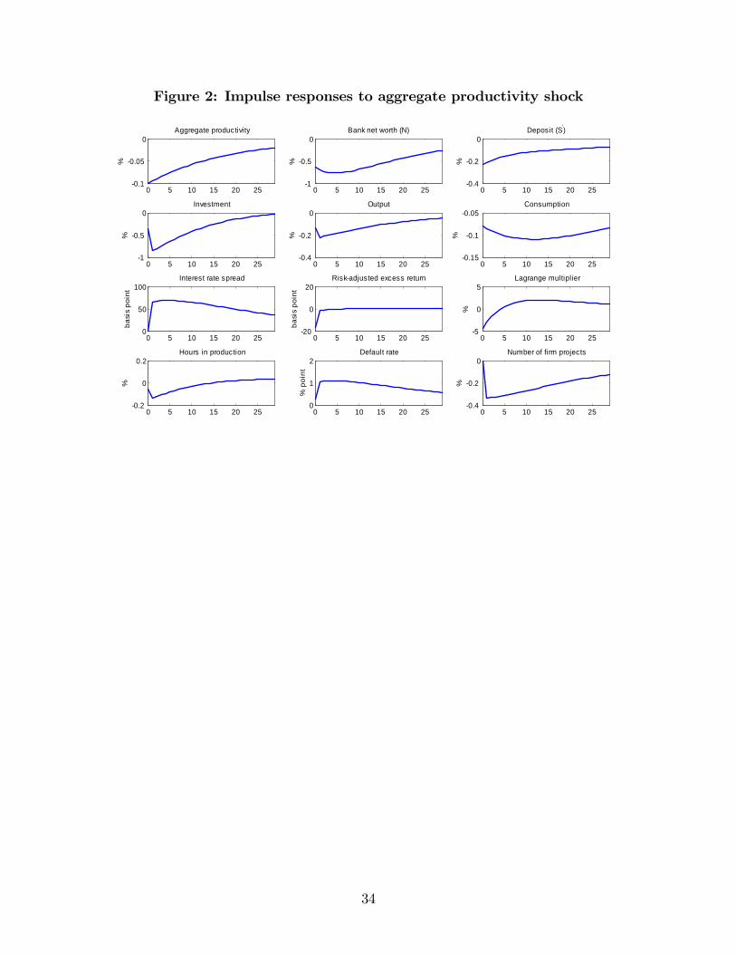
Figure 2: Impulse responses to aggregate productivity shock

0 5 10 15 20 25­0.1

­0.05

0Aggregate productivity

%

0 5 10 15 20 25­1

­0.5

0Bank net worth (N)

%

0 5 10 15 20 25­0.4

­0.2

0Deposit (S′)

%

0 5 10 15 20 25­1

­0.5

0Investment

%

0 5 10 15 20 25­0.4

­0.2

0Output

%

0 5 10 15 20 25­0.15

­0.1

­0.05Consumption

%

0 5 10 15 20 250

50

100Interest rate spread

basi

s po

int

0 5 10 15 20 25­20

0

20Risk­adjusted excess return

basi

s po

int

0 5 10 15 20 25­5

0

5Lagrange multiplier

%

0 5 10 15 20 25­0.2

0

0.2Hours in production

%

0 5 10 15 20 250

1

2Default rate

% p

oint

0 5 10 15 20 25­0.4

­0.2

0Number of firm projects

%

34

Figure 3: The role of financial frictions in propagating an aggregate productivity

shock

0 5 10 15 20 25

­0.8

­0.6

­0.4

­0.2

0

Inv es tm ent

%

0 5 10 15 20 25

­0.2

­0.15

­0.1

­0.05

0Output

%

0 5 10 15 20 25­0.12

­0.1

­0.08

­0.06

­0.04C onsum ption

%

0 5 10 15 20 25­0.4

­0.3

­0.2

­0.1

0

0.1N um ber of loans

%

NOTES: Solid lines are responses with financial frictions while dashed lines are those without

any frictions.

35

Figure 4: Impulse responses to financial shock

0 5 10 15 20 250

0.05

0.1Financial shock

%

0 5 10 15 20 250

0.2

0.4Bank net worth (N)

%

0 5 10 15 20 25­0.4

­0.2

0Deposit (S′)

%

0 5 10 15 20 25­0.5

0

0.5Investment

%

0 5 10 15 20 25­0.05

0

0.05Output

%

0 5 10 15 20 25­4

­2

0x 10 ­3 Consumption

%

0 5 10 15 20 25­50

0

50Interest rate spread

basi

s po

int

0 5 10 15 20 25­5

0

5Risk­adjusted excess return

basi

s po

int

0 5 10 15 20 25­20

0

20Lagrange multiplier

%

0 5 10 15 20 25­0.05

0

0.05Hours in production

%

0 5 10 15 20 25­1

0

1Default rate

% p

oint

0 5 10 15 20 25­0.2

0

0.2Number of firm projects

%

36

Figure 5: Prior and posterior distributions

0.1 0.2 0.3 0.40

100

0.20.40.60.8 1 1.21.40

10

2 4 6 8 100

1

2

0.7 0.8 0.9 10

10

20

0.4 0.6 0.8 10

5

ρz

σz

σψ

ρψ

σi

NOTES: Dashed and solid lines show prior and posterior distributions, respectively.

Figure 6: z and ψ measured by Bayesian estimation

Q1­90 Q1­95 Q1­00 Q1­05 Q1­10­1

­0.5

0

0.5

Aggregate Productivity (z)

%

Q1­90 Q1­95 Q1­00 Q1­05 Q1­10

­1

0

1

2

3

Financial Shock (ψ)

% p

oint

NOTES: The panels indicate percentage or percentage point deviaiton of shocks from the steady

state.

37

Figure 7: Model predictions and data

Q 1 ­ 9 0 Q 1 ­ 9 5 Q 1 ­ 0 0 Q 1 ­ 0 5 Q 1 ­ 1 0

­ 2

­ 1

0

1

2

Ou tp u t

%

Q 1 ­ 9 0 Q 1 ­ 9 5 Q 1 ­ 0 0 Q 1 ­ 0 5 Q 1 ­ 1 0

­ 4

­ 2

0

2

L a b o r i n p ro d u c ti o n

%

Q 1 ­ 9 0 Q 1 ­ 9 5 Q 1 ­ 0 0 Q 1 ­ 0 5 Q 1 ­ 1 0

­ 1 0

­ 5

0

5

1 0

P ri va te In ve s tm e n t

%

Notes: Dashed lines represent business cycle fluctuations in data; solid lines show model-implied

dynamics when feeding measured aggregate productivity and financial shocks into the model;

solid likes with circles indicate model-implied dynamics when feeding only measured aggregate

productivity shocks; solid lines with crosses represent model-implied dynamics when feeding only

measured financial shocks into the model.

38