GRE®

R E S E A R C H

February 2002

GRE Board Professional Report No. 98-01P

ETS Research Report 02-02

A General BayesianModel for Testlets:

Theory and Applications

Xiaohui WangEric T. BradlowHoward Wainer

Princeton, NJ 08541

A General Bayesian Model for Testlets:Theory and Applications

Xiaohui WangUniversity of North Carolina-Chapel Hill

Eric T. BradlowThe Wharton School, University of Pennsylvania

Howard WainerEducational Testing Service

GRE Board Report No. 98-01P

February 2002

This report presents the findings of aresearch project funded by and carried

out under the auspices of theGraduate Record Examinations Board

and Educational Testing Service.

Educational Testing Service, Princeton, NJ 08541

********************

Researchers are encouraged to express freely their professionaljudgment. Therefore, points of view or opinions stated in Graduate

Record Examinations Board reports do not necessarily represent officialGraduate Record Examinations Board position or policy.

********************

The Graduate Record Examinations Board and Educational Testing Service arededicated to the principle of equal opportunity, and their programs,

services, and employment policies are guided by that principle.

EDUCATIONAL TESTING SERVICE, ETS, the ETS logos,GRADUATE RECORD EXAMINATIONS, and GRE are

registered trademarks of Educational Testing Service.SAT is a registered trademark of the College Entrance Examination Board.

TSWE is a registered trademark of the College Entrance Examination Board.TOEFL is a registered trademark of Educational Testing Service.

Educational Testing ServicePrinceton, NJ 08541

Copyright 2002 by Educational Testing Service. All rights reserved.

i

Abstract

This paper extends earlier work (Bradlow, Wainer, & Wang, 1999; Wainer, Bradlow, & Du,

2000) on the modeling of testlet-based response data to include the situation in which a test is

composed, partially or completely, of polytomously scored items and/or testlets. A modified

version of commonly employed item response models, embedded within a fully Bayesian

framework, is proposed, and inferences under the model are obtained using Markov chain Monte

Carlo (MCMC) techniques. Its use is demonstrated within a designed series of simulations and

by analyzing operational data from the North Carolina Test of Computer Skills and Educational

Testing Service's Test of Spoken English (TSE). Our empirical findings suggest that the North

Carolina Test of Computer Skills exhibits significant testlet effects, indicating significant

dependence of item scores obtained from common stimuli, whereas the TSE exam does not.

Keywords: Bayesian hierarchical model, item response theory, polytomously scored items

ii

Acknowledgements

The authors gratefully acknowledge the support of this research by the Graduate Record

Examinations Board Research Committee, Educational Testing Service, and the College Board.

We are also grateful to Yong-Won Lee and David Thissen, who provided us with advice,

wisdom, and information functions for the summed scores of the North Carolina Test of

Computer Skills, and to Catherine Hombo for a careful reading of an earlier draft of this

manuscript. Lastly, we thank the Test of English as a Foreign Language (TOEFL) Program and

the North Carolina Department of Public Instruction, which provided us with data from the Test

of Spoken English and the North Carolina Test of Computer Skills, respectively.

iii

Table of Contents

Page

1 Introduction ............................................................................................................................. 1

2 The Model ............................................................................................................................... 3

3 Computation............................................................................................................................ 7

4 Model Testing ......................................................................................................................... 9

5 Two Tests in Need of a Scoring Model................................................................................... 13

6 Conclusions ............................................................................................................................. 22

References ................................................................................................................................... 24

List of Tables

Table 1 Table of Simulation Design.......................................................................................... 11

Table 2 Correlations Between True Parameters and Estimated Posterior Means..................... 30

Table 3 Mean Square Error Between True Parameters and Estimated Posterior Means .......... 30

Table 4 Correlations Between True Value and Posterior Mean Slope Parameter (a)............... 31

Table 5 Correlations Between True Value and Posterior Mean Difficulty Parameter (b) ........ 31

Table 6 Correlation Between True Value and Posterior Mean for Each Parameter ................. 31

Table 7 Results From Testlet Model Fitted to the North Carolina Test of Computer Skills .... 31

List of Figures

Figure 1 Information Functions for the Performance Sections of the North Carolina Test ofComputer Skills Estimated Three Ways ...................................................................... 32

Figure 2 Information From the Performance Sections of the North Carolina Computer SkillsTest Broken Down by Testlet and Showing How Each Subject Area Spans a SpecificProficiency Region....................................................................................................... 33

Figure 3 Expected Score Curves for Three TSE Items .............................................................. 34

Figure 4 The Difference in Expected Score Between the Hardest and the Easiest TSE Items.. 35

Figure 5 The Total Test Information Function for TSE Shows That the Test Provides EquallyGood Estimation Over a Very Wide Range of Proficiencies....................................... 36

Figure 6 Information Functions for All Items of the TSE; All Items Provide Uniformly HighInformation Over the Proficiency Band of Interest...................................................... 37

1 Introduction

Tests are typically made up of smaller components - items - which act in concert to measure .

the test designers’ constructs of interest. Over the last half century one of the most important

theoretical innovations in test theory has been a family of statistical models that characterize, in .

a stochastic way, the event of an exaxninee meeting an item (Birnbaum, 1968; Lord, 1952; 1980;

Rasch, 1960). Underlying all versions of these item response models is the assumption that there

exists an unobservable, latent proficiency (usually denoted 8 ) for each examinee which determines

(in conjunction with parameters about the items) that exam&e’s likelihood of success on a given

item. In practice, when utilizing item response models, it is always assumed that responses to

all items are independent of one another after conditioning on the underlying, latent examinee

proficiency. Experience has shown that when tests are made up of separate, unrelated items this

assumption of conditional independence (CI) is sufliciently close to being true to allow these models

to be of great practical usefulness. There are, however, some reasonably common circumstances in

which the assumption of CI is not likely to be true.

The most frequent such circumstance observed in practice is when a test is constructed of

“testlets.” A testlet (Wainer & Kiely, 1987) is defined as an aggregation of items that are based on

a single stimulus, such as in a reading comprehension test. In this case, a testlet might be defined as

the passage and the set of four to 12 items that accompany the passage. It is not hard to imagine,

therefore, that issues such as misinterpretation of the passage, subject matter expertise, fatigue,

and so on would cause responses to these items to be more highly related than suggested by the

overall (omnibus) latent proficiency for the entire test. In some sense, this lack of CI is a form of

unidimensional proficiency model misfit, which may be explainable by the test structure (i.e., the

testlet design). It is the incorporation of this test design structure into a formal probability model

that motivated this research.

Much previous work exists in the psychometric literature on the modeling and/or detection of

testlet dependence. Under the heading of “appropriateness measurement,” Drasgow, Levine, and

Williams (1985) and Levine and Drasgow (1988) describe parametric approaches for identification of

deviations from standard unidimensional item response models. In more recent work, Stout (1987)

and Zhang and Stout (1999), develop nonparametric approaches (e.g., the DETECT statistic) to

determine when proficiency unidimensionality is likely to be violated. The previous research most

relevent to the present work-by Bradlow, Wainer, and Wang (1999) and Wainer, Bradlow, and

Du (2000)-proposes a parametric Bayesian model for item test scores composed of a mixture of

binary independent and testlet items. Their base models, which are a modification of standand item

response models (two and three parameter logistic models) that include an additional interaction

term for persons answering a given testlet, demonstrate that (a) both examinee proficiencies and

item parameters are biased when testlet dependence is ignored; (b) the amount of testlet dependence

varies across testlets; and (c) testlet dependence exists in operational tests. However, their work

assumes that each item response is binary; in the current study, we address an extension to that

assumption motivated by the increasing number of operational tests that are composed of a mixture

of binary and polytomous items, both independent and nested within testlets.

This extension is important for practical as well as theoretical reasons. First, tests with this

format are in use, and existing scoring models that do not take into account within-testlet depen-

dence will yield overly optimistic estimates of the test’s overall precision. Therefore, we expect

that mixed format tests with testlets models (a term we coin for tests composed of a mixture of

binary and polytomous items, some independent and some within testlets) and related estimation

procedures can have immediate operational use, such as with Educational Testing Service’s (ETS)

Test of Spoken English (TSE) and various achievement exams given very widely.

Secondly, some recent research has shown that richer inferences and diagnostic proficiency in-

2

formation can be obtained using portfolios (Advanced Placement Studio Art), essays, and other

types of constructed responses, which are scored polytomously. As this belief becomes more ac-

cepted, and as such test items become more common, we expect models with the capability of

the one proposed here to be widely used. In addition, as testlets composed of one item are single

dependent items, by definition, our model easily simplifies to the standard model assuming CL

The remainder of this manuscript is laid out as follows. In Section 2, we describe in detail our

Bayesian parametric model for mixed binary-polytomous test with testlets. Section 3 contains a

description of the computational approach utilizing a Markov chain Monte Carlo (MCMC) sampler.

A large scale simulation study demonstrating the efficacy of our approach under a wide range of

realistic test conditions is provided in Section 4. In Section 5 we apply our model to operational data

from the North Carolina Test of Computer Skills (details can be found in pdf “Assessment brief’ at

http://www.dpi.state.nc.us/accountability/testing/computerskills/index.html) and ETS’s Test of

Spoken English (TSE) exam (Educational Testing Service, 1995). These applications demonstrate

both the existence of testlet effects in some cases and not in others, and the operational feasibility

of our approach. Summary conclusions are given in Section 6. A small technical appendix with

details of our implementation of an MCMC sampler is also provided.

2 The Model

As our model must encompass both binary and polytomous items, two basic (and widely used)

probability kernels drove our approach: the three-parameter logistic model for binary items (Bim-

baum, 1968), and the polytomous item response model introduced by Samejima (1969). These

models are given respectively by:

Pij(l) = P(lhj = 110, wj) = Cj + (1 - cj)logit-‘(tij), and

3

(1)

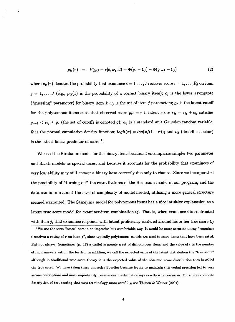
Pij(r) = P(Yij = 40, mjj d) = a(& - tij) - @(gr_l _ tij) (2)

where pij(r) denotes the probability that exam&e i = 1, . . . , I receives score r = 1, . . . , Rj on item

j=l,..., - J (e.g., pij(l) is the probability of a correct binary item); cj is the lower asymptote

(“guessing” parameter) for binary item j; wj is the set of item j parameters; gr is the latent cutoff

for the polytomous items such that observed score yij = r if latent score sij = tij + Gj satisfies

gr_r < sij 5 gr (the set of cutoffs is denoted 9); ej is a standard unit Gaussian random variable;

4i? is the normal cumulative density function; Zogit(z) = Zog(z/(l - z)); and &j (described below)

is the latent linear predictor of score ‘.

We used the Birnbaum model for the binary items because it encompasses simpler two-parameter

and Rasch models as special cases, and because it accounts for the probability that exam&es of

very low ability may still answer a binary item correctly due only to chance. Since we incorporated

the possibility of “turning ofP’ the extra features of the Birnbaum model in our program, and the

data can inform about the level of complexity of model needed, utilizing a more general structure .-

seemed warranted. The Samejima model for polytomous items has a nice intuitive explanation as a

latent true score model for examinee-item combination ij. That is, when exam&e i is confronted

with item j, that exam&e responds with latent proficiency centered around his or her true score tij

‘We use the term “score” here in an imprecise but comfortable way. It would be more accurate to say “examinee

i receives a rating of t on item j”, since typically polytomous models are used to score iterns that have been rated.

But not always. Sometimes (p. 17) a testlet is merely a set of dichotomous items and the value of T is the number

of right answers within the testlet. In addition, we call the expected value of the latent distribution the “true score”

although in traditional true score theory it is the expected value of the observed score distribution that is called

the true score. We have taken these imprecise liberties because trying to maintain this verbal precision led to very

arcane descriptions and most importantly, because our mathematics says exactly what we mean

description of test scoring that uses terminology more carefully, see Thissen & Wainer (2001).

4

For a more complete

with random error qj. Observed score yij = r occurs when the latent score is within an estimated

(latent) range [gr_r , gr]. The ability of our approach to model extra dependence due to testlets,

first described in Bradlow et al. (1999), is obtained by extending linear score predictor tij from its

standard form:

t ij = Uj(6i - bj) (3)

where aj , bj , and 0i have their usual interpretations as item slope, item difhculty, and exam&e

proficiency to:

t ij = aj(ei - bj - %d(j)) (4

where %d( j ) is the testlet effect of person i to item j nested in testlet d(j). The extra dependence

of items within the same testlet for a given exam&e is modeled in this manner, as both would

share the effect yid(j) in their score predictor. By definition, ~ido) = 0 for all independent items,

or testlets of size one.

Using these kernels as a base, we supposed the following general testing set-up to fully explicate

our model. Suppose I examinees each take an examination composed of J items, where J = .I&+ Jp,

and Jb is the number of binary items in the test while Jp is the number of polytomous items.

Furthermore, let Jb denote the set of binary items and ,& the set of polytomous items. We further

suppose that each of the J items are nested within K testlets; that is, d(j) E (1,. . . , K}, where

kd(j) and b(j) denote the number of items and sets of items nested within testlet d(j). Under this

paradigm, and using the probability kernels given in equation (1) and (2), we obtain the likelihood

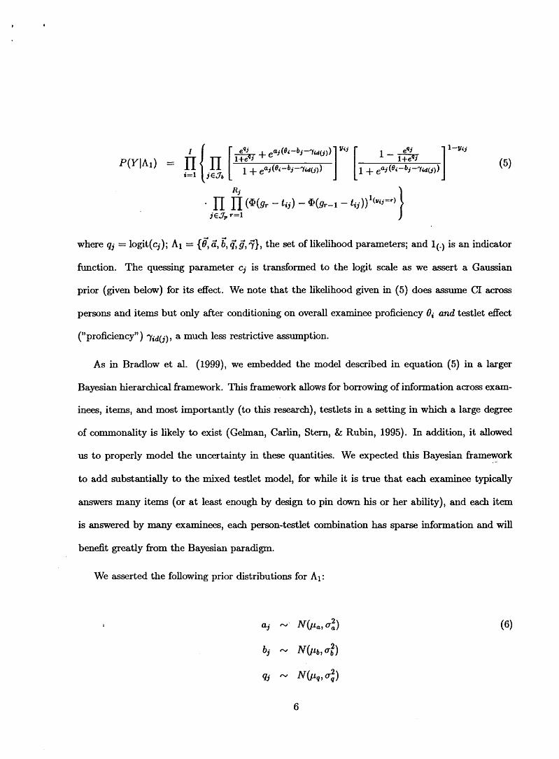
for observed test score matrix Y = (gij) given by:

5

&+e [ .

Uj(ei_bj_7a(j)) yij 1 _ eqj l_Yij

iiz 1 + ,+(ei_bj_7ti(j))

I[ 1 + euj(ei-aj-7aG)) 1 (5)

l I-J n w!Jr - tij) - $(f&_l - tij))l(Wzr)

jG& r=l

where Qj = lOgit( Al = (3 , ii, & $, G, q}, the set of likelihood parameters; and l(.) is an indicator

function. The quessing parameter cj is transformed to the logit scale as we assert a Gaussian

prior (given below) for its effect. We note that the likelihood given in (5) does assume CI across

persons and items but only after conditioning on overall exam&e proficiency Oi and testlet effect

(fiproficienc$) Tid(j), a much less restrictive ~~ption.

As in Bradlow et al. (1999), we embedded the model described in equation (5) in a larger

Bayesian hierarchical framework. This framework allows for borrowing of information across exam-

inees, items, and most importantly (to this research), testlets in a setting in which a large degree

of commonality is likely to exist (Gehnan, Carlin, Stern, & Rubin, 1995). In addition, it allowed

us to properly model the uncertainty in these quantities. We expected this Bayesian tiamework

to add substantially to the mixed testlet model, for while it is true that each exam&e typically

answers many items (or at least enough by design to pin down his or her ability), and each item

is answered by many exam&es, each person-testlet combination has sparse information and will

benefit greatly from the Bayesian paradigm.

We asserted the following prior distributions for Al:

6

. .

%d( j)

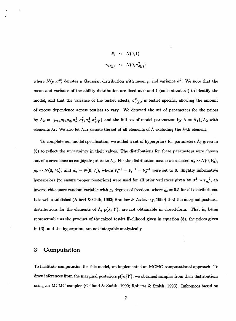
where iV(p, cr2) denotes a Gaussian distribution with mean ~1 and variance 02. We note that the

mean and variance of the ability distribution are fnced at 0 and 1 (as is standard) to identify the

model, and that the variance of the testlet effects, g2 d(j), is testlet specific, allowing the amount

of excess dependence across testlets to vary. We denoted the set of parameters for the priors

bY A-2 = {PO, Pb, Pg, ci> ui, 0:~ O& } and the full set of model parameters by A = Ar UA2 with

elements XI;. We also let A_k denote the set of all elements of A excluding the Ic-th element.

To complete our model specification, we added a set of hyperpriors for parameters A2 given in

(6) to reflect the uncertainty in their values. The distributions for these parameters were chosen

out of convenience as conjugate priors to A 1. For the distribution means we selected pa N N(0, V,),

pb - N(0, &,), and pQ N N(0, &), where V;l = V,-’ = Vq,’ were set to 0. Slightly informative

hyperpriors (to ensure proper posteriors) were used for all prior variances given by crz N xk2, an

inverse &i-square random variable with gz degrees of freedom, where gz = 0.5 for all distributions.

It is well established (Albert & Chib, 1993; Bradlow & Zaslavsky, 1999) that the marginal posterior

distributions for the elements of A, $)(&I Y), are not obtainable in closed-form. That is, being

representable as the product of the mixed testlet likelihood given in equation (5), the priors given

in (6), and the hyperpriors are not integrable analytically.

3 Computation

To facilitate computation for this model, we implemented an MCMC computational approach. To

draw inferences from the marginal posteriors p(&lY), we obtained samples from their distributions

using an MCMC sampler (Gelfand & Smith, 1990; Roberts & Smith, 1993). Inferences based on

7

posterior means, quantiles, interesting posterior probabilities, and so on were then derived from

sample-based estimates. The standard MCMC approach-to begin with some starting value, A(‘),

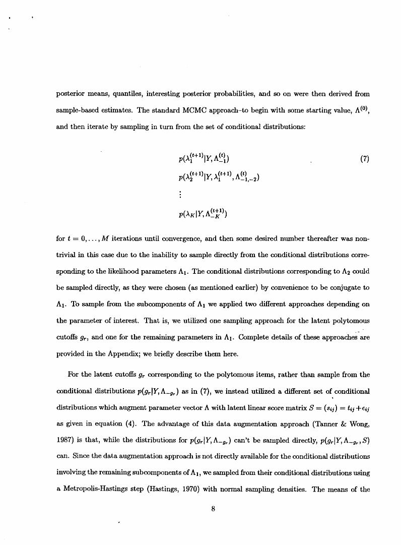
and then iterate by sampling in turn from the set of conditional distributions:

p(p)lY, A’_“‘,)

p($+')IY A @+1) AI”‘, 11 ’ ,-

2)

for t = O,... , M iterations until convergence, and then some desired number thereafter was non-

trivial in this case due to the inability to sample directly from the conditional distributions corre-

sponding to the likelihood parameters 111. The conditional distributions corresponding to A2 could

be sampled directly, as they were chosen (as mentioned earlier) by convenience to be conjugate to

Al. To sample from the subcomponents of Ar we applied two d&rent approaches depending on

the parameter of interest. That is, we utilized one sampling approach for the latent polytomous

cutoffs gr, and one for the remaining parameters in AI. Complete details of these approaches are

provided in the Appendix; we briefly describe them here.

For the latent cutoffs gr corresponding to the polytomous items, rather than sample from the

conditional distributions p(gJY, A_& as in (7)) we instead utilized a different set of conditional

distributions which augment parameter vector A with latent linear score matrix S = (sij) = tij +eij

as given in equation (4). The advantage of this data augmentation approach (Tanner & Wong,

1987) is that, while the distributions for p(grlY, A_gr) can’t be sampled directly, p(grlY, A_st, S)

can. Since the data augmentation approach is not directly available for the conditional distributions

involving the remaining subcomponents of Ar , we sampled from their conditional distributions using

a Metropolis-Hastings step (Hastings, 1970) with normal sampling densities. The means of the

8

, ,

sampling densities were set to the previously drawn value Xtt) A: , and the variance was set adaptively

to achieve a high acceptance rate (Gelman, Roberts, & Gilks, 1996). Although, a single approach

(Metropolis-Hastings) could h ave been used to sample all subcomponents of Ar, a comparison (not

reported) between Metropolis-Hastings for all parameters and the data augmentation approach for

the cutoffs indicated that applying both algorithms would be superior.

4 Model Testing

To check both accuracy and computational time for realistic size data sets, and to understand the

impact of dependence in the mixed testlet model, we conducted extensive simulations using our

computational approach. We performed our simulation study for two primary purposes. First, we

wanted to confirm that we could obtain accurate estimates of the model parameters under wide

variation of three experimental factors; that is, we sought realistic values likely to be seen in practice.

As this procedure will have operational utility, practical application of this methodology was of

critical importance. Second, we wished to compare our results with current standard estimation

approaches in the testing industry specifically, those using MULTILOG (Thissen, 1991).

In testing the model and our estimation approach, we considered three experimental factors,

denoted Factors A, B, and C. Factor A was the number of categories (nc) for each item. Thus for

dichotomous items n, = 2, and for polytomous items, we manipulated the number of score levels

n, > 2. Factor B, testlet length or q, was defined as the number of items within a testlet. Finally,

factor C, the variance of the testlet effects, c;(j), indicated the degree of within-testlet dependence,

as in (6).

Niie different simulation conditions were studied, using a data generation computer program

developed for this purpose. For each of the nine conditions, five data sets were simulated indepen-

9

dently for a total of 45 simulated data sets. Each data set consisted of responses of 1,000 simulees

to a test of 30 items. Among those 30 items, 12 were independent dichotomous items (i.e., not

within testlets), and the remaining 18 were dichotomous and polytomous testlet items. Of course,

as the 12 independent, binary items contained no testlet effect by definition (&&, = 0), and had a

fixed number of categories (n, = 2), our simulation manipulations corresponded to variations in the

remaining 18 items.

independent binary

Placement Program

This test design was utilized to mimic many current operational tests in which

multiple-choice items are followed by essay/portfolio testlets (e.g., Advanced

tests).

Because a 33 design with 27 combinations would have been too computationally “expensive” to

run, and because our interests predominantly lay in estimating main effects and two-way interac-

tions, a Latin Square design was employed to cover the variation of these three factors. For Factor

A, we chose the number of response categories to be 2, 5, or 10, corresponding to binary items

and to polytomous items scored on 5 and 10 point scales, respectively. Thus, if n, = 2, the entire

test is binary (including the 12 independent items and the 18 testlet items), and this mimics the

work of Wainer, Bradlow, and Du (2000). For Factor B, we designated the length of the testlets as _-

three items, six items, and nine items, respectively. Since we fixed the total number of testlet items

at 18, these assignments corresponded to six testlets, three testlets, and two testlets. Therefore,

Factor A times Factor B yielded nine combinations. For Factor C, the variance of testlet effects, we

chose its values to 0.0 (i.e., no testlet effect), 0.5 ( small variance), and 1.0 (bigger variance). Since

8 w N(0, 1) to identify the model, all values of ~~~j~ are relative to 1, the variance of the person

abilities. Using the Latin Square design, we let Factor C change for each level of Factors A and B.

Table 1 describes our simulation design.

From previous work of Wainer, Bradlow,

MCMC estimation approach) containing only

and Du (2000), we knew that this model (and the

binary items (conditions 1, 4, and 7) works very well

10

Factor C Factor A

Variance of Testlet Effect 2 categories 5 categories 10 categories I I I

6 testlets I 0.0 (1) ) 0.5 (2) I 1.0 (3)

-Factor B 3 testlets 1 0.5 (4) 1 1.0 (5) 1 0.0 (6)

2 testlets 1 1.0 (7) 1 0.0 (8) 1 0.5 (9)

Note: Numbers from l-9 in parentheses indicate our labeling of the

simulation conditions and are used throughout.

Table 1: Table of Simulation Design

for situations with a positive and a zero testlet effect. Under the design in Table 1, we expected

that our procedure would give accurate estimates for the item parameters, including the cutoffs gr

for the categories of polytomous items, regardless of the number of categories n,, the testlet length

nt, and the variance of the testlet effects.

To make the simulated test data as similar as possible to real world applications, we selected

population distributions for the parameters used to generate the data that correspond to previ-

ous analyses of the SAT examination. Specifically, we used 6$ - N(0, l), aj - N(1.5, 0.452),

bj - N(0, l), and cj - N(0.14, 0.052). The population distributions for uj were left-truncated at

0.3, and those for cj were left-truncated at 0.0 and right-truncated at 0.6. 2

2For practical usage, when aj is too small (as estimated from calibration samples), that implies a very low item

discrimination (i.e., the item slope is too low, indicating that the item is unable to meaningfully differentiate people

with varying abilities) and such items are never used; they are pruned from the test. Similarly, as cj are guessing

parameters, when items are guessed correctly too often, the items are pruned. Such truncations were not critical to

our simulation design and did not occur that frequently; equally accurate results were obtained in test NILS without

these restrictions.

11

, .

All 45 simulated data sets were analyzed by our procedure. The estimated parameters were

then compared in various ways with the true model parameters to determine whether the procedure

recovered their values. The estimated parameters were posterior means of the MCMC draws for

each parameter obtained from the last 1,000 draws of a single MCMC chain of length 3,000. The

initial 2,000 draws were discarded as an initial burn-in period.

We assessed the performance of our model using two criteria: the correlation between the

estimated parameters and the true parameters, and the mean square error of the estimates from

the true values. The full results are presented in Table 2 and Table 3, respectively. Each value

in these tables represents asl average over the five replications for that condition. For ease of

presentation, the values in Table 3 are multiplied by 100. Appended to Table 2 are rearranged

subtables (Tables 4, 5 and 6), which explicitly reflect the main effects embedded in the structure

of the experimental design. We have only included those tables in which the main effects varied

meaningfully with the values of an independent variable.

INSERT TABLES 2,3,4,5,6 HERE

Table 2, shows that our procedure provided very accurate estimates for item difficulty (a) and

cutoff (gr) parameters (average correlations of 0.992 and 0.980 respectively) across all simulation

conditions. The average correlation equals 0.93 for the ability parameters 8 and 0.89 for the

discrimination (a) parameters. As is typical with IRT models, the procedure’s ability to estimate

the guessing parameters was more modest; in this case, the average correlation is 0.60. This

was expected because there are very few simulees whose proficiency is low enough to provide

information in the estimation of the guessing parameter (c). The magnitude of the correlations

were all consistent with our prior beliefs based on past research. The differences in these correlations

across the various levels of the design were small, but consistent, for some parameters.

12

In Table 4, we see that the accuracy of estimation of the slope parameter (a) increased with

the number of items within a testlet (since test length was fixed, as the number of testlets nt

was reduced their average length was, perforce, increased). This was expected since with longer

testlets there is more data available for the slope estimates. We also found increased precision as

the number of categories, n,, for each polytomous item increased.

We found a similar effect on the difficulty parameter (b), shown in Table 5. This parameter was

so well estimated that it was difficult for any variation in the independent variables to have much

effect. Last, when we examine the effect of varying the testlet parameter-var (7) in Table 6-we

find that only slope (a) and proficiency (0) showed any consistent effect (albeit not statistically

different); in both cases, increasing testlet effect decreased precision.

An analysis of the mean square errors (Table 3) shows almost exactly the same pattern. Using

our model, i item parameters were well estimated, with average squared prediction error ranging

from a low of 0.006 (0.60 x 10 -2 from Table 3) for the difficulty parameters, to a high of 0.054

(5.4 x 10e2 Erom Table 3) for the guessing parameters. Simulee abilities were also extremely well

estimated, with MSE equal to 0.001 (1.0 x 10e2). The same main effects between precision and

independent variables shown in Table 2 and its subtables reappeared in Table 3, but now when

considering mean square error (MSE).

5 Two tests in need of a scoring model

Next, we applied our approach, now validated, to the analysis of operational data from two tests

made up of testlets: the North Carolina Test of Computer Skills, one section of which is composed of

four testlets that turned out to show very large testlet effects, and the TSE exam, which is composed

of four testlets that manifested essentially none of the excess local dependence that is typical of

13

testlet-based tests. Our analyses demonstrate how the use of our new model allows accurate scoring

when its generality is needed, and how it still provides important and useful information even when

its generality appears not to be needed.

Test 1. North Carolina Test of Computer Skills. The North Carolina Test of Computer Skills

is given to 8th graders and must be passed as a requirement for graduation from junior high

school. It was developed to help ensure basic computer proficiency for graduates of the North

Carolina Public Schools, and is made up of two parts. The first part of the exam is presented in

a standard multiple-choice format, and the second part is performance based, consisting of four

testlets that deal with keyboarding, word processing/editing, database use, and spreadsheet use.

The keyboarding portion includes three polytomous items scored on a four-point scale, while the

word processing/editing, database, and spreadsheet testlets include six to 10 items scored either

dichotomously or trichotomously. Each student receives two separate scores-one for the multiple-

choice portion and one for the performance portion-and is required to pass both parts.

In their analysis of the performance section, Rosa, Swygert, Nelson, and Thissen (2001) found

that that the reliability of the computer skills test, assuming no testlet effects, was 0.83, whereas

when the test was scored as being made up of four testlets, its reliability was 0.65. If all of the items

measure the same trait and there is no excess local dependence (testlet effect), we would expect

that an estimate of the test’s reliability based strictly on the items (ignoring the testlet structure)

would be the same as an estimate based on the testlets. The result obtained suggests that there is

substantial within-testlet dependence. To assure an honest estimate of the precision of the test, it

would seem that some other test scoring model, beyond a standard model assuming CI, should be

.

used.

Our testlet model is sufficiently general to allow the entire exam to be scored together. Such

an approach has some important advantages when a total exam, like this one, is predominantly

14

unidimensional (Rosa et al. 2001). Principal among these advantages is that a single score for the

two parts combined would yield a more reliable measure of a student’s computer proficiency.

Although providing a single score was technically feasible, the strategy of computing two sepa-

rate scores and requiring the student to pass both parts was adopted for at least two reasons-the

first economic, the second technical. The economic reason was that the performance portion of

the test is very expensive to administer, so the students take the cheap part (the multiple-choice

section) over and over again until they pass it. Then they take the performance part until they

pass it. The hope was that the extra study involved in the retesting of the multiple-choice section

would reduce the number of times that the performance part needed to be taken. There is some

evidence that this is true. At the very least, those that never pass the first part never take the sec-

ond. The technical reason for providing two scores was that, until now, no rigorous scoring model

was available that could mix all parts together in an optimal fashion-although there certainly were

methods for doing it fairly well (Rosa et al. 2001).

We fit the testlet model given in Equation (5) and (6) to the performance data from one

administration of the North Carolina test. The test was administered during the 199495 school

year as part of an item tryout. The tryout included potential performance items arranged into

12 forms numbered 13-24; the data used in the current study was from form number 13, which

included 26 items divided into testlets as shown in Table 7. The sample size for this form was 266,

roughly one twelfth of the 3,099 examinees with complete data in the field test.

An MCMC sampler was run from three starting points for 3,000 draws each. The first 2,000

draws from each chain were discarded, and the remaining draws were used for inference. The last

column of Table 7 presents the estimated values of the testlet effects var(r). The interpretation of

the size of the testlet effects is aided by remembering that they are on the same scale as exam&e

proficiency. Thus a testlet effect of one means that the variance associated with local dependence

15

is of the same order of magnitude as the variance of examinees’ ability. We see that there were very

large testlet effects for the word processing/editing portion of the test as well as the spreadsheet

section. This reflects the highly interconnected nature of these tasks. There was a smaller, but

nevertheless substantial, effect for database use. Only the keyboarding section seemed to yield

independent items.

INSERT TABLE 7 HERE

The simulation results discussed in Section 4 indicated that having a substantial testlet effect

will not affect the accuracy of some of the parameters, but it will affect testlet and total test

information; I(0) = - E(d210gL/M2), h w ere L is (for our model) the mixed testlet model likelihood

given in Equation (5). It is worthwhile to compare the results for test information we obtained

from our model with what was yielded by two traditional approaches. As expected, a comparison

of estimated proficiencies 8 across methods indicated a correlation above 0.95 and hence are not

reported in detail here. Test information in test theory, as in many applications, is critical, in that

it informs the level of certainty of ability estimation at varying levels of ability.

Figure 1 presents three information curves. The highest curve was obtained by fitting an

IRT model to the individual items of the North Carolina test and assumed that the items are

conditionally independent (setting var(r) equal to zero), and by using MULTILOG. The middle

curve was estimated using our MCMC output. Specifically, J(0) was computed pointwise for 106

equally spaced grid points of 8 between -3 and +3 for each of the draws of the sampler. The value

for I(0) under our model for each grid point was then computed as average information over the

draws. The computational formula for I(e) for each item under our mixed-testlet model was easily

derived from Equation (5)) and can be shown to be equal to

16

4 (p$r - 1) - &r))2 4Ce) = C

r=r Ptjtr - l) - PrjCr)

a special case of the formula given in Baker (1992; page 241, equation 8.19), where

(8)

Pitj (r) = C+>r pij (r) with pij (r), as given in Equation (2) for polytomous items and in Equation

(1) for dichotomous ones, and p:‘(r) is its respective derivative. That is, p~j(r) is the cumulative

probability of being greater than r under the model, and hence, pi;(r) - &(r - 1) = pij (r). The

lowest curve was obtained by treating each testlet as a single polytomous item and only record-

ing the total number of points assigned, also using MULTILOG. This latter approach has been

widely used (Thissen, Steinberg, & Mooney, 1989; Wainer, 1995), but as we see here, it tends to

be too conservative; by using only the total score it loses any information that is carried in the

exact pattern of responses. In summary, Figure 1 indicates that ignoring the testlet effect provides

standard errors inversely related to test information that will be potentially too small under the

Cl assumption and too large when collapsing testlet data into a single score.

INSERT FIGURE 1 HERE

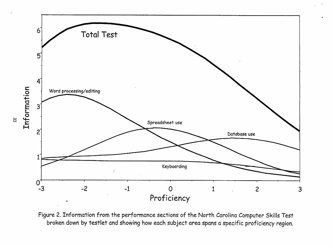
One further finding from the North Carolina analysis bears mention. Figure 2 shows information

curves for each of the testlets, as well as the total test’s information curve. This display makes

absolutely clear the relationship between testlet topic and the proficiency levels at which that topic

provides information. The word processing/editing section of the North Carolina test provides its

peak information for examinees at the lowest proficiency levels, whereas the section on database

use is focused at the highest proficiency levels. Interestingly, the limited value of the keyboarding

section is distributed pretty uniformly across the entire proficiency range. These findings of highly

differentiated testlets are in stark contrast to our findings for the Test of Spoken English, shown

next.

17

INSERT FIGURE 2 HERE

Test 2. The Educational Testing Service’s Test of Spoken English. A second example of the

same sort of testlet design manifests itself in the TSE exam, the primary purpose of which is to

measure the ability of normative English speakers to communicate orally in English. TSE scores

are widely used by North American institutions for the selection of teaching assistants and doctoral

students. They are also used outside of academia in many selection and certification circumstances,

most commonly in the health professions for physicians, nurses, pharmacists, and veterinarians.

The TSE is made up of some independent items and three testlets, which themselves are com-

posed of polytomous items3. Each testlet requires a particular language function (i.e., narrating,

recommending, persuading), and is composed of a stimulus (e.g., a map, a sequence of pictures, a

graph) and related items. After having the opportunity to study the stimulus, a series of orally pre-

sented questions about that stimulus are posed. The test is delivered on an audio tape augmented

by a test booklet, and the examinee’s responses are recorded on a separate answer tape.

Each TSE item is scored by two expert raters on a nine-point rating scale. If raters differ by

more than one point on average over the 12 items scored, a third rater is brought in to adjudicate.

The ratings of the two closest raters are then averaged and summed to provide the final score.

We fit our model to Form 3VTSOl of the TSE, which was administered in January of 1999.

A total of 2,127 individuals took the test at that time. We transformed their scores onto a scale

that ranges from 20 to 60, with the various levels interpreted in terms of the ability to effectively

30f the 12 items on the test: Testlet I is made up of items 1 through 4 which are based on the same map; Testlet

II is made up of items 5 through 8, which are based on a series of pictures; item 9 is a discrete item that asks

the examinee to summarize some information of the speaker’s own choosing; Testlet III is made up of items 10 and

11, which are based on the same graph; and item 12 is a discrete item that provides a train schedule and requires

exam&es to give instructions to someone who needs to get somewhere.

18

communicate in English. These levels are shown .

Score Level

60

50

40

30

20

Communication Ability In English

Almost always effective

Generally effective

Somewhat effective

Not generally effective

No effective communication

Our results indicate that the current practice of having raters score each item and then just

adding them up as if they were independent is not unreasonable. We reached this conclusion when

we found that there was essentially no excess local dependence on this form of the TSE [var(+y) < .04

for all testlets]. Because the size of the testlet effects was so small, we concluded that the current

practice of ignoring it when calculating test summaries was completely justified for this form of

the test. We can only speculate about whether all TSE forms show this same characteristic. Our

experience with other tests (e.g., the North Carolina Test of Computer Skills and the Law School

Admissions Test, to pick two) suggests that an absence of t&let effects is the exception, not the

rule. In a separate research project currently underway, we are collecting testlet covariates (e.g.,

passage length, topic domain, and so on) to aid test developers in creating priori assessments of

which testlets are likely to violate of CI (and their extent). As ultimately total test information at

a minimum level is desired, this should have great practical importance.

After fitting our model to the TSE data, we used MCMC draws to construct the expected score

curves for each item, E(vij 1 Ait’). Figure 3 s h ows the expected score curves (averaged over the draws

hit)) for three items: the easiest (item l), the hardest (item 9), and the item of median difficulty

(item 5). Each of these items was meant to test different aspects of English proficiency, which were

19

anticipated to become increasingly sophisticated as the test progressed. As Figure 3 shows, gigantic

differences in expected score did not occur at any level of proficiency, but the biggest differences

occured at a very low level of proficiency (0 = - 1.75). This could be seen more clearly when we

plotted the difference in expected score between item 1 and item 9 in Figure 4. As is expected,

at very low and very high levels of proficiency there are no differences in performance among the

items. At the prior mean proficiency level (6= 0), there is only a four point difference in expected

score between the most difficult and easiest item.

It turns out that all other items fall within this envelope. One interpretation of this result

is that, once an individual’s proficiency reaches a level characterized as “somewhat effective” the

INSERT FIGURES 3 and 4 HERE

various aspects of linguistic proficiency spanned by this test are of almost equal difhculty. This was .

apparently suspected by the language experts who construct the TSE exam, but they had never

been able to find compelling evidence to support this suspicion. Our model provided this evidence.

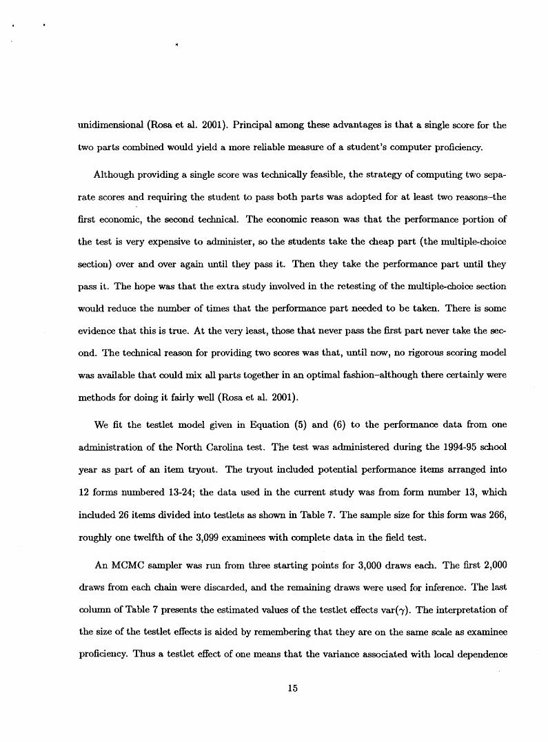
As part of our analysis, we also looked at the information function, as in Equation (8); for

the entire TSE test. We found that the area of peak accuracy of the test is remarkably broad

(see Figure 5). Thus, this form of the TSE yields equally accurate measurement across a very

broad spectrum of examinee proficiencies, encompassing fully 84% of the examinee population. An

information function as flat as this is unusual. It represents a real success from a test design point

of view, for it means that a very large proportion of exam&es are tested with equal accuracy.

Typically, information functions for fixed format tests peak in the middle and taper off quickly on

both sides. Only adaptive tests (Wainer, Dorans et al. ZOOO), which are individually constructed

to be optimal for each exam&e, can be counted on to yield information curves like this one on

a regular basis. Using test information (or its inverse, the standard error) as a representation of

20

accuracy is likely to be far more useful than a single reliability statistic.

INSERT FIGURE 5 HERE

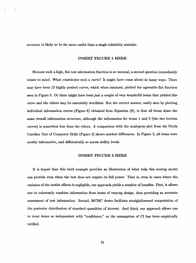
Because such a high, flat test information function is so unusual, a second question immediately

comes to mind. What constitutes such a curve? It might have come about in many ways. There

may have been 12 highly peaked curves, which when summed, yielded the agreeable flat function

seen in Figure 5. Or there might have been just a couple of very wonderful items that yielded this

curve and the others may be essentially worthless. But the correct answer, easily seen by plotting

individual information curves (Figure 6) obtained from Equation (8), is that all items share the

same overall information structure, although the information for items 1 and 2 (the two bottom

curves) is somewhat less than the others. A comparison with the analogous plot from the North

Carolina Test of Computer Skills (Figure 2) shows marked differences. In Figure 2, all items were

mostly informative, and differentially so across ability levels.

INSERT FIGURE 6 HERE

It is hoped that this brief example provides an illustration of what help this scoring model

can provide even when the test does not require its full power. That is, even in cases where the

variance of the testlet effects is negligible, our approach yields a number of benefits. First, it allows

one to coherently combine information from items of varying design, thus providing an accurate

assessment of test information. Second, MCMC draws facilitate straightforward computation of

the posterior distribution of standard quantities of interest. And third, our approach allows one

to treat items as independent with “confidence,” as the assumption of CI has been empirically

verified.

21

6 Conclusions

The North Carolina Test of Computer Skills and the TSE are testlet-based tests in which at least

some of the items are polytomously scored. While there are psychometric models that can fit tests

made up of polytomous items (e.g., Sarnejima, 1969; Bock, 1972), there are no psychometric models

currently available that can accommodate such tests when within-testlet local dependence is likely.

In both our simulations and our analysis of real data, we have shown how this model can be used

to score such tests and provide estimates of test precision that are neither as optimistic as models

that incorrectly assume conditional independence nor as pessimistic as those that only use total

score. Furthermore, we have shown that in some cases testlet structures yield local dependence,

while in other cases they yield none. As mentioned earlier, examining predictors of this sort will

likely be of great practical interest.

There are currently two trends in modern testing. The first is a movement away from what is

viewed as the atomistic nature of discrete multiple-choice items and toward the use of testlets as

a way of providing context. The second is toward computerizing tests, both to allow the testing

of constructs difficult or impossible to test otherwise, and to imprave the efficiency of tests by

making content adaptive to individal proficiency. Adaptive tests are often engineered to stop after

measuring exam&e proficiency to a predetermined level of precision. The model that we have

proposed and tested here, by allowing the inclusion of testlets scored in a variety of ways, and

therefore providing accurate assessments of information, should prove to be a useful complement

to these modern trends.

Our model can have immediate application in many testing programs, but its principal value

lies in the future. It provides a mechanism for scoring a test that is made up of any combination

or grouping of multiple-choice items, fill-in-the-blank items, and other constructed-response items

22

that are judged by expert raters. This means that test developers can focus on what test structure

measures best the construct of interest and trust that there will be an appropriate scoring model

available for it. This has not been the case in the past.

Our analyses of the North Carolina Test of Computer Skills show one situation in which this

testlet scoring model is required. The analysis of the TSE exam provides assurance that current

test scoring methods are adequate. But there are also other instances in which this model can be

profitably and immediately employed. For example, consider the Graduate Record Examinations

(GRE) Writing A ssessment, in which examinee writing samples are scored by two judges. If those

judges disagree strongly, a third judge-a “master rater”-is brought in. The exam&e’s final score

is the average of the master rater’s judgment and the judge that is closest to the master rater. This

approach is wasteful of expert judgment. We can be more efficient by using the new model. Let us

think of the essay and its associated polytomous ratings as a single testlet in which the judges are

the “items.” We can then leave in all of the raters and allow the model to assign weights to the

raters that are proportional to the extent to which each rater’s judgment is related to the common

underlying trait. This is theoretically akin to the observed score approach espoused by Braun and

Wainer (1989).

Because this model is so general, its potential uses are very broad indeed. Although the re-

quirements implicit in building testlets adaptively were the driving forces behind the development

of the model, that is only one of its areas of application. Others will emerge as test developers’

eyes grow accustomed to the light that is shed by this approach.

Perhaps the greatest value of this model is the role that it will play as the foundation of a

general educational diagnostic system. As the model is currently configured, it can answer many

“how much” questions: How much ability does this exam&e have? How much difficulty does

this item have? How much local dependence exists within this testlet? These are often important

23

questions, but for diagnosis as well as scientific understanding, we need answers to a similar set of

“why” questions: Why does this exam&e show this much ability? Why is this item so difficult?

Why does this testlet exhibit so much local dependence ? To answer such questions, one further

generalization in which each of the parameters of interest is decomposed into a function of covariates

is required. The developments discussed here are necessary precursors to this ultimate goal.

References

Albert, J. H., & Chib, S. (1993). Bayesian analysis of binary and polychotomous response data.

Journal of the American Statistical Association, 88, 669-679.

Baker, F. B. (1992). Item response theory. New York, NY: Marcel-Dekker Inc.

Birnbaum, A. (1968). S ome latent trait models and their use in inferring an examinee’s ability. In

F. M. Lord and M. R. Novick (Eds.), Statistical theories of mental test SWTVS (pp. 397-479).

Reading, MA: Addison-Wesley.

Bock, R. D. (1972). Estimating item parameters and latent ability when responses are scored in

two or more latent categories. Psychometrika, 31; 29-51.

Bradlow, E. T. & Wainer, H. (1998). Some statistical and logical considerations when restoring

tests. Statistica Sinica, 8, 713-728.

Bradow, E. T., Wainer, H., & Wang, X (1999). A Bayesian random effects model for testlets.

Psychometrika, 64, 153-168.

Bradlow, E. T., & Zaslavsky, A. M. (1999). A hierarchical latent variable model for ordinal data

from a customer satisfaction survey with “no answer” responses. Journal of the American

Statistical Association, 94, (445), 43-52.

24

Braun, H. & Wainer, H. (1989). Making essay test scores fairer with statistics. In J. Tanur et al.

(Eds.), Statistics: A guide to the unknown (3rd ed., pp. 178-187). San Francisco, CA: Holden

Day.

Drasgow, F., Levine, M. A., & Williams, E. A. (1985). Appropriateness measurement with poly-

chotomous item response models and standardized indices. The British Journal of Mathematical

Psychology, 38, 67-86.

Educational Testing Service (1995). TSE scof’e user’s manual.

Service.

Princeton, NJ: Educational Testing

Gelfand, A. E., & Smith, A. F. M. (1990). Sampling-based approaches to calculating marginal

densities, Journal of the American Statistical Association, 85, 398-409.

Gelman, A., Carlin, J. B., Stern, H. S. & Rubin, D. B. (1995). Bayesian data analysis. London:

Chapman & Hall.

Gelman, A., Roberts, G, & Gilks, W. (1995). Efficient metropolis jumping rules. In J. M. Bernardo,

J. 0. Berger, A. P. Dawid, & A. F. M. Smith (Eds.), Bayesian statistics

Oxford University Press.

Gehnan, A., & Rubin, D. B. (1992). Inf erence from iterative simulation using

Statistical Science, 7, 457-511.

5. New York, NY:

multiple sequences,

Hastings, W. K. (1970). Monte Carlo sampling methods using Markov chains and their applications.

Biometrika, 54, 93- 108.

Levine, M. V. AZ Drasgow, F. (1988). Optimal appropriateness measurement. Psychometrika, 53,

161-176.

Lord, F. M. (1952). A theory of test scores. Psychometric Monographs, 1

25

Lord, I?. M. (1980). Applications of item response theory to practical testing

NJ: Lawrence Erlbaum.

pmblems. Hlllsdale,

Roberts, G. ,O., & Smith, A. F. M. (1993). Bayesian computation via the Gibbs Sampler and

related Markov chain Monte Carlo methods. Journal of the Royal Statistical Society, Series B,

55, 3-23.

Rosa, K., Swygert, K., Nelson, L. & Thissen, D. (2001). Item response theory applied to combi-

nations of multiple-choice and constructed response items: Scale scores for patterns of summed

scores. D. Thissen and H. Wainer (Eds.), T es scoring (pp. 253-292). Hillsdale, NJ: Lawrence t

Erlbaum.

Samejima, F. (1969). E t s imation of latent ability using a response pattern of graded scores. Psy-

chometrika Monographs, 17.

Stout, W. F. (1987). A nonparametric approach for assessing latent trait dimensionality. Psy-

chometrika, 52, 589-617.

Tanner, M. A., and Wong, W. H. (1987). The calculation of posterior distributions by data aug-

mentation. Journal of the American Statistical Association, 82, 528540.

Thissen, D. (1991). MULTILOG user’s guide (version 6). Mooresville, n\J: Scientific Software.

Thissen, D., Steinberg, L. & Mooney, J.A. (1989). Tr ace lines for testlets: A use of multiple-

categorical-response models. Journal of Educational Measurement 26, 247-260.

Thissen, D. & Wainer, H. (Eds.) (2001). Test Swting. HXlsdale, NJ: Lawrence Earlbaum ASSO-

ciates.

Wainer, H., Bradlaw, E. T., & Du, 2 (2000). Testlet response theory. An analog for the 3-PL

useful in testlet-based adaptive testing. In W. J. van der Linden & C. A. W. Glas (Eds.),

26

. .

Computeriaed adaptive testing: Theory and practice. Kluwer-Nijhoff, 245-270.

Wainer, H. & Kiely, G. (1987). Item clusters and computerized adaptive testing: A case for testlets.

J~umal of Educational Measumment, 24, 185-202.

Wainer, H. (1995). Precision and differential item functioning on a k&let-based test: The 1991 Law

School Admissions Test as an example. Applied Measurement in Education, 8, (2), 157-187.

Wainer, H., Dorans, N., Eignor, D., Flaugher, R., Green, B., Mislevy, R., Steinberg, L. & Thissen,

D. (2000). Computerized adaptive testing: A pn’mer (2nd ed.). Hillsdale, N. J.: Lawrence

Erlbaum.

Zhang, J. & Stout, W. F. (1999). The theoretical DETECT index of dimensional&y and its appli-

cation to approximate simple structure. Psychometrika, 64, 213-249.

27

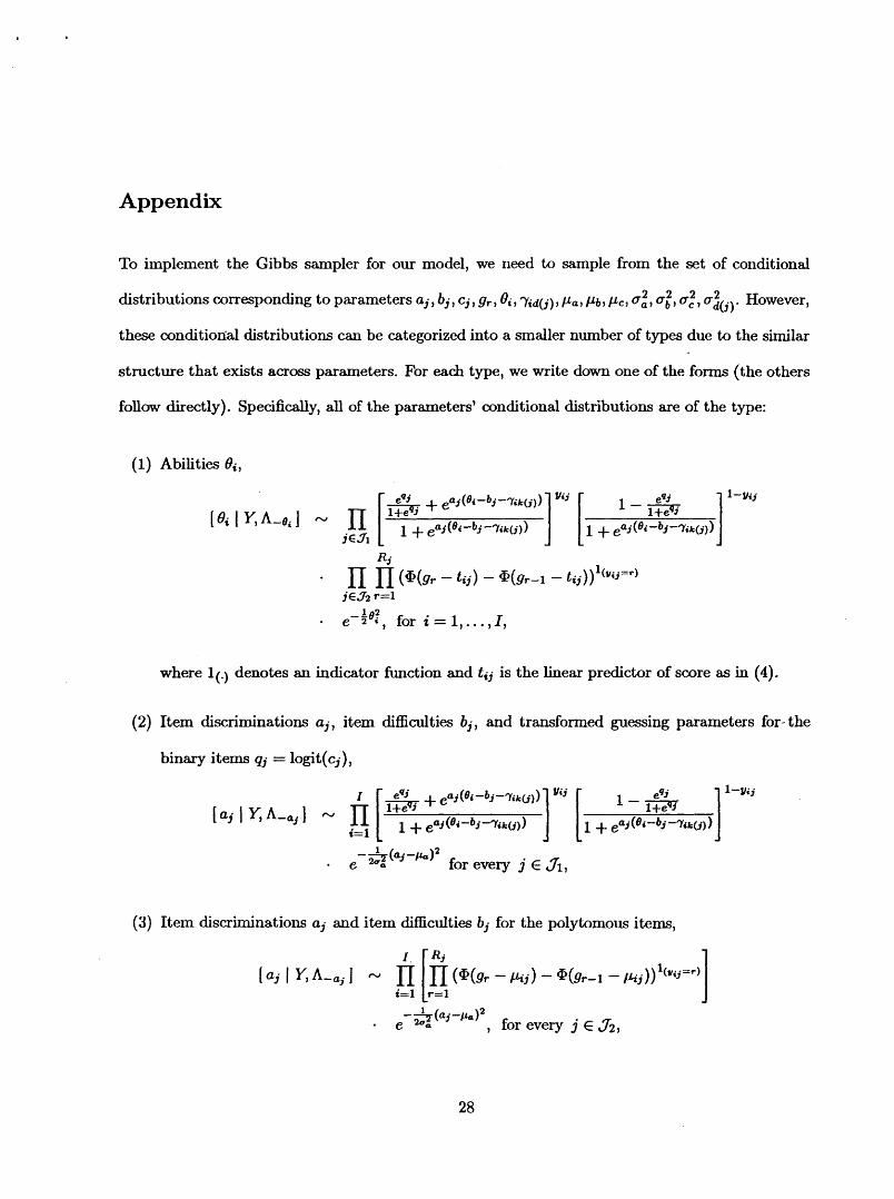
Appendix

To implement the Gibbs sampler for our model, we need to sample from the set of conditional

distributions corresponding to parameters CZ~, bj, Cj, gr, 6i, Tid(j), pa, pb, pC, 02, c$, 6,2, ~~(j). However,

these conditional distributions can be categorized into a smaller number of types due to the similar

structure that exists across parameters. For each type, we write down one of the forms (the others

follow directly). Specifically, all of the parameters’ conditional distributions are of the type:

(1) Abilities Oi,

,_&& + euj(&-bj-.-rqj))

1 + eaj(ei_bj_7ik(j))

1 _ eqj l-l&j

-

1 + ,aj(ei_bj_7iko)) 1

. e-2 lez, for i=l,..., I,

where It.1 denotes an indicator function and tij is the linear predictor of score as in (4).

(2) Item discriminations Uj , item difficulties bj, and transformed

binary items qj = logit(

guessing parameters for- the

1 _ eQi l--Yij

iTi3 1 + eaj(ei-bj-7uqj))

1

. e-*(aj-b)2 for every j E $1,

(3) Item discriminations aj and item difficulties bj for the polytomous items,

[aj 1 Y,A-tZj] - (%J r

-+(aj-_Cra)2 . e 2ba 9 for every j E 32,

28

(4)

(5)

(6)

(7)

Testlet effects ~~~~0’1,

’ [ Tik I K ‘-vi, ] c3 n[ .$+e aj(Oi-bj-rir;(j)) vij

i EOVl 1 + ,aj(ei-bj-%k(j)) 1 [

1 _ eqj l--Yij

I+e’Jj

1 + ,aj(ei-aj-Tik(j)) 1 Rj

.

rI b

(@(CJT - tij) - @(&__l - tij))l(uii=rJ *

jEn&n& f-1 1 -+$k . e y(k) forevery i=l,..., I, and k=l,..., K,

Polytomous item cutoffs,

UIlifO~IXl(XIltlX{tij : Yij = ~},min{tij : Yij = r + I}),

uniform random variable.

Prior means Par CLb, Pq,

[ /Ja ] Y, A_,, ] Oc e-a(fi-“2, 1 J

where ti = - J c aj,

j=l

a normal random variable.

Prior variances f12 c2 c2 f12 a’ 69 q’ d(k),

[ 4 I WL~]

N u;2[($+f)-lJe-~i2 [i+$ ~&(aj-pa)2] 1

a;n inverse-gamma random variable.

As we note in text for the current study, distributions for forms (l), (2), (3), and (4) were

obtained using a Metropolis-Hastings step. Draws from (5), (6), and (7) were obtained directly from

uniform, normal, and inverse-gamma distributions respectively. Computation for each iteration of

the sampler took l/3 second for simulated data consisting of 1,000 simulees, and roughly 1.5 seconds

per iteration for real data examples run on a Pentium 3, 550 MHZ computer programmed in C.

29

Table 2: Correlations Between True Parameters and Estimated Posterior Means.

Simulation Number of Number of Number Categories Testlets

1 2 6 2 5 6 3 lo- 6 4 2 3 5 5 3 6 10 3 7 2 2 a 5 2 9 10 2

mr(7) 0.0 0.5 1.0 0.5 1.0 0.0 1.0 0.0 0.5

0.891 70.051) 0.886 (0.036) 0.846 (0.093) 0.832 (0.054) 0.891 (0.063) 0.951 (0.013) 0.870 (0.054) 0.927 (0.051) 0.939 (0.010)

b 0.990 (0.003) 0.993 (0.003) 0.993 (0.004) 0.992 (0.002) 0.995 (0.002) 0.994 (0.002) 0.984 (0.003) 0.992 (0.004) 0.995 (0.002)

0.635 [O. 101) 0.660 (0.123) 0.565 (0.134) 0.645 (0.098) 0.600 (0.140) 0.619 (0.128) 0.500 (0.103) 0.633 (0.208) 0.536 (0.073)

lc 0.972 (0.013) 0.973 (0.006)

NA 6.984 (0.007) 0.986 (0.007)

NA 0.979 (0.007) 0.986 (0.007)

Note: Reported values are the average over five replicated data sets. Values in parentheses are corresponding standard deviations. NA values indicate those cases in which all items were binary and hence cutoffs did not have to be estimated.

Table 3: Mean Square Error Between True Parameters and Estimated Posterior Means.

e 0.924 (0.005) 0.947 (0.006) 0.934 (0.005) 0.911 (0.003) 0.902 (0.015) 0.979 (0.004) 0.884 (0.015) 0.972 (0.005) 0.916 (0.009)

Simulation Number

Number of Number of Categories Testlets

2 6 5 6 10 6 2 3 5 3 10 3 2 2 5 2 10 2

m(7) 0.0 0.5 1.0 0.5 1.0 0.0 1.0 0.0 0.5

1.54 TO.31) 1.46 (0.48) 2.29 (1.19) 1.47 (0.20) 1.20 (0.53) 0.79 (0.14) 1.80 (0.41) 0.97 (0.46) 0.92 (0.36)

b

0.75 (0.33) 0.46 (0.13) 0.52 (0.18) 0.68 (0.31) 0.34 (0.12) 0.50 (0.36) 1.29 (0.55) 0.55 (0.30) 0.48 (0.17)

5.52 Fl.38) 3.50 (1.04) 6.12 (3.04) 5.25 (1.46) 4.00 (1.56) 3.84 (1.74) 9.87 (5.22) 4.57 (2.59) 4.94 (2.16)

L 0.96 (0.52) 2.34 (0.70)

NA 0.48 (0.19) 1.17 (0.50)

0.63;. 15) 1.19 (0.46)

8 0.14 (0.01) 0.11 (o.olj 0.13 (0.01) 0.18 (0.01) 0.18 (0.02) 0.04 (0.01) 0.21 (0.02) - 0.06 (0.01) 0.16 (0.02)

Note: Reported values are the average over five replicated data sets. Values in parenthesis are corresponding standard deviations. All table values are multiplied by 102. NA values indicate those cases in which all items were binary and hence cutoflh did not have to be estimated.

30

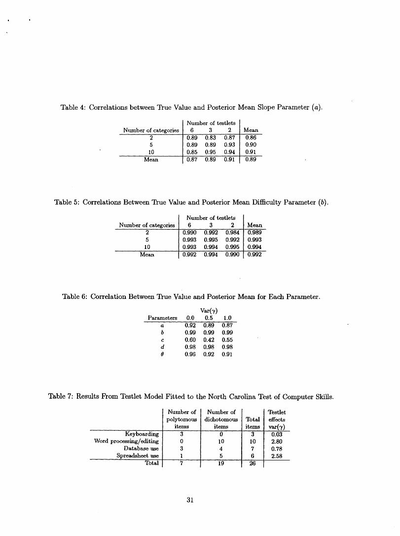
Table 4: Correlations between True Value and Posterior Mean Slope Parameter (a).

_ ~

Table 3: Correlations Between True Value and Posterior Mean Difficulty Parameter (b).

Table 6: Correlation Between True Value and Posterior Mean for Each Parameter.

Wr) Parameters 0.0 0.5 1.0

a 0.92 0.89 0.87

b 0.99 0.99 0.99

: 0.60 0.98 0.98 0.42 0.55 0.98

8 0.96 0.92 0.91

Table 7: Results From Testlet Model Fitted to the North Carolina Test of Computer Skills.

Keyboarding

items

3

items

0

items var(7)

3 0.03

Number of

I

Number of

I I

Testlet

polytomous dichotomous Total effects

Word processing/editi~ I 0 I 10 I 10 I 2.80

Database use 3 4 7 0.78

Spreadsheet use 1 5 6 2.58

Total 7 19 26

31

E .- t d E t 0

2 H

10

5 ti fnfnrmntinn tnkina testlet

/

m.., _. .I._, ._.. ._* . . . . J . --. .-.

effects into account

[var(y)estimated J

Information using only the

testletsummedscores

0; I I I 1 1 a’

-3 -2 -1 0 1 2 3

Proficiency

Figurel. Information functions fortheperfor'mancesections of the North CarolinaTestof Computer Skills estimatedinthreeways.

-3 -2

u

-1 0

Proficiency 1 2

Figure Z.Informationfromtheperformancesections of the North CarolinaComputer Skills Test

broken down bytestletandsho6ving how each subjectareaspans aspecific proficiency region.

60

u Ql $ 35

Ql p 30

UJ

25

Item 1

- Item

- Item 9

_____--___ -_--_---_--__--___

generdy

I I

__-__---_--__-____ Communicatibnsomewhat __-_--___________

I effeitive I I I

I I

comnjunication

-3 -2 *’ -1 0 1

Proficiency

Figure 3. Expectedscorecurves for three TSEitems

a

7

6

5

4

3

2

1

0 -4 -3 -2 -1 0 1 2 3

Proficiency

Figure 4. The difference in expected score between the hardest \

and the easiest TSE items.

40

30

20

10

C

-3 -1 0 1 - 2 3

Proficiency

Figure 53hetotaltestinformation function for TSEshowsthatthetestprovides equally

good estimation overaverywide rangeof proficiencies.

4

0

Each curve represents the information

from oneofthe12 TSEitems

-3 -2 -1 0

Proficiency

. 1 2 3

Figure 6.Information functions for all items of the TSE; all items provide uniformly high informationover the proficiency band of interest.