A Gauss—Newton method for convex composite...

Mathematical Programming 71 (1995) 179-194

A Gauss-Newton method for convex composite optimization 1

J.V. Burke a, M.C. Ferris b'* a Department of Mathematics, GN-50, University of Washington, Seattle, WA 98195, United States

b Computer Sciences Department, University of Wisconsin, 1210 West Dayton Street, Madison, W1 53706, United States

Received 28 September 1993; revised manuscript received December 1994

Abstract

An extension of the Gauss-Newton method for nonlinear equations to convex composite optimization is described and analyzed. Local quadratic convergence is established for the minimization of h o F under two conditions, namely h has a set of weak sharp minima, C, and there is a regular point of the inclusion F ( x ) E C. This result extends a similar convergence result due to Womersley (this journal, 1985) which employs the assumption of a strongly unique solution of the composite function h o F. A backtracking line-search is proposed as a globalization strategy. For this algorithm, a global convergence result is established, with a quadratic rate under the regularity assumption.

Keywords: Gauss-Newton; Convex composite optimization; Weak sharp minima; Quadratic convergence

1. Introduction

In the early nineteenth century, Gauss proposed a powerful method for solving systems

of nonlinear equations that generalized the classical Newton's method for such systems.

Recall that Newton's method is based on successive linearization. Unfortunately, in

many applications the linearized systems can be inconsistent. To remedy this problem,

Gauss proposed that the iterates be based on the least-squares solutions to the linearized

problems. In making the transition from solving the linearization to solving the associated

* Corresponding author, e-mail: [email protected]. l This material is based on research supported by National Science Foundation Grants CCR-9157632 and

DMS-9102059, the Air Force Office of Scientific Research Grant F49620-94-1-0036, and the United States- Israel Binational Science Foundation Grant BSF-90-00455.

0025-5610 @ 1995--The Mathematical Programming Society, Inc. All rights reserved SSDI 0025-56 10(95)00010-0

180 J.V. Burke, M.C. Ferris/Mathematical Programming 71 (1995) 179-194

linear least-squares problem, the underlying problem changes from equation solving to minimization. Specifically, the Gauss-Newton method solves the associated nonlinear

least-squares problem and can therefore converge to a solution to the nonlinear least- squares problem that is not a solution to the underlying system of equations. Nonetheless, the method is always implementable and can be made significantly more robust by the addition of a line-search. Other variations that enhance the robustness of the method are the addition of a quadratic term to the objective in the step-finding subproblem (see [20,27] ) or the inclusion of a trust-region constraint (see [ 13] ).

In this paper we discuss the extension of the Gauss-Newton methodology to finite- valued convex composite optimization. Convex composite optimization refers to the minimization of any extended real-valued function that can be written as the composition of a convex function with a function of class C1 :

(79) rain f ( x ) : = h ( F ( x ) ) ,

where h : R m --+ R t_l {+ec} is convex and F : lt~" ~ R m is of class C 1 . We consider

only the finite-valued case: h : R m -+ R. Obviously the nonlinear least-squares problem is precisely of this form. It is interesting to note that in their outline of the Gauss- Newton method, Ortega and Rheinboldt [28, p. 267] used the notion of a composite function. A wide variety of applications of this formulation can be found throughout the mathematical programming literature [6,16,17,21,31,39,40], e.g., nonlinear inclusions, penalization methods, minimax, and goal programming. The convex composite model provides a unifying framework for the development and analysis of algorithmic solution techniques. Moreover, it is also a convenient tool for the study of first- and second-order

optimality conditions in constrained optimization [ 7,9,17,39 ]. Our extension of the Gauss-Newton methodology to finite-valued convex composite

optimization is based on the development given in [5,18], which specifically address the problem of solving finite-dimensional systems of nonlinear equations and inequalities. In this case, much more can be said about the algorithmic design and this is done in the cited articles. In this article we focus on the general theory. Specifically, we extend a result due to Womersley [40] establishing the quadratic convergence of a Gauss- Newton method under the assumption of strong uniqueness. An important distinction between these results is that we do not require that the solution set be a singleton or even a bounded set. A further discussion of the relationship to Womersley's result is

given at the end of Section 3. The approach we take requires two basic assumptions: (1) the set of minima for the

function h, denoted by C, is a set of weak sharp minima for h, and (2) there is a

regular point for the inclusion

F ( x ) C C. (1)

In this article, we provide a self-contained and elementary proof theory in the finite-

dimensional case. The basic algorithm is discussed in Section 2. After a discussion of regularity in Section 3, we establish the local quadratic convergence of the method in

J.V. Burke, M.C. Ferris/Mathematical Programming 71 (1995) 179-194 181

Section 4. The results of Section 4 can be extended to the setting of reflexive Banach spaces under a suitable strengthening of the regularity condition (see condition (10) ). We conclude in Section 5 by establishing the convergence properties of a globalization strategy based on a backtracking line-search.

The notation that we employ is for the most part standard; however, a partial list is provided for the readers' convenience. The inner product on R", (y, x), set addition U ± flV and set difference U \ V are standard. The polar of U C R" is the set U ° := {x* E R" I (x*, x) ~< 1, Vx E U}. The relative interior of U, ri U, is the interior of U relative to the affine hull of U and the closure of U, cl U, is the usual topological closure of the set U. The cone generated by U is cone(U) := {,~u I A > 0, u c U}. The indicator function for U is the function ~bu(x) taking the value 0 when x is in U and +ec otherwise. The support function for U is given by ~p{j(x) := sup{(x*,x) I x* E U}.

We denote a norm on R ~ by II' II, its closed unit ball by ~, and its dual norm by IIx[lo := ~b~ (x). It is straightforward to show that the unit ball associated with the dual

norm is II~ °. The distance of a point x to a set U is given by dist(x ] U) := inf{llx -ull I u E U}. Finally, the sets ker A and im A represent the kernel and image space of the linear map A, respectively, and the inverse image of a set U under the mapping A is given by A-1U : = {y I Ay ~ U}.

2. The basic algorithm

Let f ( x ) := h ( F ( x ) ) be as given in (7 ~) with h finite-valued. The basic Gauss- Newton procedure takes a unit step along a direction selected from the following set:

D~(x) := argmin{h(F(x) + V ' ( x )d ) I Ildll (2)

which represents the set of solutions to the minimization problem

min{h(F(x) + F ' ( x ) d ) [ Ildll ~< d}. (3)

There are two points to note. The first is that the "linearization" is carried out only on the smooth function F, the convex function h is treated explicitly, corresponding exactly to the Gauss-Newton methodology. The second point is that the directions are constrained to have length no greater than A. This is different from the standard Gauss- Newton procedure which can be recovered by setting A = oc. Nonetheless, from the standpoint of convergence analysis it is advantageous to take A finite. Observe that D,a is a multifunction taking points x and generating a set of directions. The basic algorithm to be considered here is as follows.

Algorithm 1. Let ~/ /> 1, A E (0, +cx~] and x ° E R n be given. Having x k, determine x k+l as follows.

If h(F(xk ) ) = min{h(F(x k) + U ( x k ) d ) [ IId[[ ~< ~), then stop; otherwise, choose d k C D,a(x k) to satisfy

Ildkl[ ~< ~Tdist(OID~(xk)), (4)


and set x k+l := x k + d k.

Algorithms of this type have been extensively studied in the literature [5,t8,23,33].

I f it is assumed that both h and the norm on ]1{ n are polyhedral, then one can obtain

a direction choice satisfying (4) in Algorithm 1 by computing a least-norm solution

of a linear program in the sense of [24,25]. Numerical methods for obtaining least-

norm solutions to linear programs have been developed in [ 12]. I f h is piecewise linear-quadratic and the norm on R n is either polyhedral or quadratic, then a two-stage

procedure can be employed to obtain the step d k. In the first stage one obtains an optimal

solution to (3) , dopt, then in the second stage a least-norm solution is obtained by solving

the linear or quadratic program min{]]dtl I F' (x )d = F'(x)dopt}. For example, when the norm on R '~ is polyhedral, the algorithm given in [2] will solve (3). If h is the distance

function to a nonempty closed convex set, one can apply the relaxation techniques

described in [5] .

In most studies, the objective function in (3) includes a quadratic term of the form

½dTHd in order to incorporate some curvature components. Such methods are commonly

referred to as sequential quadratic programming methods. In addition to a second-order

sufficiency condition, these methods require a strong nondegeneracy condition for their

local analysis. These conditions combine to imply that the point under consideration is an

isolated stationary point of the problem. Consequently, this theory does not apply to the

class of problems addressed in this article. Further discussion of this curvature component

can be found in [13,28] for the classical Gauss-Newton method and in [17,31] for

convex composite optimization. The relationship of this component to second-order

optimality conditions can be found in [9,17,39]. In this article, we avoid the need for a

curvature term by focusing on the local behavior of the algorithm in the neighborhood

of a point 2 satisfying F(.~) C C := argminh, assumed nonempty. Our analysis is based on two key assumptions: the set C is a set of weak sharp

minima for the function h and the point 2 is a regular point (see Section 3) for the

inclusion (1). The weak sharp minima concept was introduced in [ 14].

Definition 2.1. The set C C R m is a set of weak sharp minima for the function h : R m --~ R t3 {±oc} if there is an ce > 0 such that

h(y) )hmin + a d i s t ( y I C) , for all y E ]I{ m, (5)

where hmin := miny h(y). The constant ce and the set C are called the modulus and domain of sharpness for h over C, respectively.

Note that in finite dimensions, if inequality (5) is satisfied for one choice of norm,

then it is satisfied for every other norm with perhaps a different choice of ce. The pro-

totypical example of a function h having a set of weak sharp minima is the distance

function dist(. I C) itself; other examples are explored in [8,14]. The notion of weak

sharp minima generalizes the notion of a sharp [30] or strongly unique [11,21,29,40] minimum. These concepts have a long history in the literature and have far-reaching con-

J.V. Burke, M.C. Ferris/Mathematical Programming 71 (1995) 179-194 183

sequences for the convergence analysis of many iterative procedures [ 11,19,21,30,40]. In [ 8 ], it was shown that some of these convergence results can be extended to the case

of weak sharp minima. This article continues this discussion in the context of convex composite optimization. Whereas in the fully convex case one obtains finite termination criteria, in the convex composite case we can establish quadratic convergence when regularity is also assumed.

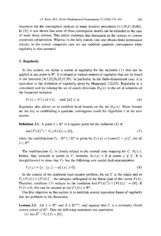
3. Regularity

In this section, we define a notion of regularity for the inclusion (1) that can be applied at any point in R n. It is related to various notions of regularity that can be found

in the literature [4,7,22,26,35,37,39]. In particular, in the finite-dimensional case, it is equivalent to the definition of regularity given by Maguregui [22,23]. Regularity is a convenient tool for relating the set of search directions Da(x) to the set of solutions of the linearized inclusion

F(x ) ÷ F ' ( x ) d E C, with Ildll ~< A. (6)

Regularity also allows us to establish local bounds on the set Dz(x ) . These bounds are the key to establishing a quadratic convergence result for Algorithm 1 in the next

section.

Definition 3.1. A point 2 C R" is a regular point for the inclusion (1) if

k e r ( U ( 2 ) T) n F c ( F ( 2 ) ) = {0}, (7)

where the multifunction Fc : R m ~ R"' is given by F c ( y ) := [cone(C - y ) ]o , for all y E R m.

The multifunction Fc is closely related to the normal cone mapping for C, N c ( ' ) .

Indeed, they coincide at points in C; however, N c ( y ) = 0 at points y ¢ C. It is straightforward to show that Fc has the following very useful dual representation:

rc(z) = {Yl (y ,z) - ~O~(y) >>. 0}. (8)

In the context of the nonlinear least-squares problem, the set C is the origin and so Fc ( F ( 2 ) ) = [ F ( 2 ) ] ±, the subspace orthogonal to the linear span of the vector F(2) . Therefore condition (7) reduces to the condition k e r ( F t ( 2 ) T) N [ F ( 2 ) ] ± = {0}. I f

F(2) = 0, this can be restated as i m ( F t ( 2 ) ) = ]R m. Our first objective in this section is to establish several equivalent forms of regularity

that are pertinent to the discussion.

L e m m a 3.2. Let Z ¢ N m and A ¢ R mxn, and suppose that C is a nonempty closed

convex subset of R m. Then the following statements are equivalent. (i) ker,~ f N F c ( Z ) = {0}.


(ii) imfi, + cone ( r iC - Z) = R m.

(iii) There is a tz > 0 such that

0 c int(/zABn + ( r iC - g ) ) ,

where B, is the unit ball of R n.

(iv) There is a /3 > 0 such that

--I o (,,~T) B,, r~ Cc(~ ) c/3B°,. (9)

(v) There is an e > 0 such that each of the conditions ( i ) - ( i v ) above hoM for all (z, A) C (Z, ,~) + •B where the unit ball in R m x ~mxn is determined by the norm

I I ( z , m ) - ( Z , ~ ) I I - - I I z - zll + l[ m - fi']l

with the operator norm on R mx" chosen to be compatible with the given norms on ~n

and ]~m. In particular, the parameters tz in (iii) and/3 in (iv) depend only on the point

(~ ,A) .

Proof. To obtain the equivalence of (i) and (ii) , we first take the polar of the relation in (i) to see that imfi~ + c l c o n e ( C - Z) = R m. From this equation, the equivalence follows from a simple separation argument and the fact that r i coneS = cone (ri S) for

any convex set S. Clearly, (ii) follows from (iii) . The reverse implication again follows by a simple

separation argument. Indeed, if this implication were false, then one could separate the origin from the set # A B , + (ri C - g) , for each Iz > 0. But then the cone generated by these sets, namely im,~ + cone ( t iC - g ) , would lie in a half space which would contradict (ii) .

To see that (iv) follows from (iii), note that (iii) is equivalent to the statement

that there exists an 77 > 0 such that r/Bin C /z.,~B,, + (ri C - Z). This implies that (rl/Iz)B,,, C .~B, + cone (C - ~). The polar of this last expression is precisely (iv)

wi th/3 =/xr / -~.

Clearly, (iv) implies (i) since kerfi, = (/~T)-10 and the only bounded cone is the origin.

For the final statement of the lemma, it is obvious that (v) implies any one of ( i ) - ( iv) . We obtain the equivalence of (v) with any one of ( i ) - ( i v ) by showing that (iii) implies the local version of ( iv) . This will simultaneously establish the uniform nature of the parameter /3. First, it is clear that if (iii) holds for some A, ~ and /2, then it holds for all A, z and /z nearby. As noted above, the condition in (iii) implies the

existence of an r / > 0 and / z > 0 such that r/Nm C/zABn + (ri C - g) . Hence, r/Bin C # A B , + (ri C - z ) + ½r/N,~,, whenever (z, A) E (Z, fi~) + e B , for some • > 0. Therefore, by the R~dstrOm Cancellation Lemma [32, Lemma 1], l'r]Bm C /.tAN, + ( r iC - z) which implies that r//(2/z)B,,, C A B , , + cone (C - z) . Taking the polar of this last statement and set t ing/3-1 := z/ / (2/z) , we find that (iii) implies the existence of • > 0

and/3 > 0 such that the condition in (iv) holds for all ( z ,A) E (g ,A ) + • B . []

J.E Burke, M.C. Ferris/Mathematical Programming 71 (1995) 179-194 185

Remarks. ( 1 ) Maguregui [ 22,23 ] studies methods similar to Algorithm 1 in the Banach space setting under the regularity condition

0 C core(( imA + C - g)) . (10)

This condition and condition (ii) of Lemma 3.2 are equivalent in the finite-dimensional setting. In the infinite-dimensional setting, (10) is stronger than the condition in (ii), but condition (ii) is not strong enough to obtain Maguregui's sensitivity results.

(2) By taking A = U ( 2 ) and g = F(2) , Lemma 3.2(v) implies that ker ( U ( x ) T) N F c ( F ( x ) ) = {0} for all points x near 2 at which (7) holds. That is, regularity is a local property.

The following proposition can be viewed as a local Hoffman bound for the linearized inclusions (6). This result is similar to [35, Theorem 1]. Our proof is a straightforward application of Fenchel's Duality Theorem [38, Corollary 31.2.1]. It is self-contained and significantly simplifies the proof technique employed in [ 35, Theorem 1 ] which depends on the theory of normed convex processes [34]. The power of this approach for the derivation of very general Hoffman bounds is illustrated further in [ 10].

Proposition 3.3. If 2 is a regular point of (1), then for all A > dist(O I D ~ ( 2 ) ) , there is some neighborhood N' (2) of 2 and a fl > 0 satisfying

dist(0 } D o ( x ) ) <<. f ld i s t (F(x) I C) , (11)

whenever x E iV'(2). Moreover, .A[(2) can be chosen so that there exists d E A~ satisfying

F (x ) + F ' ( x ) d E tiC, (12)

for all x ~ N'(2) .

Proof. We first establish (11). Let • > 0 be given by Lemma 3.2(v) at the pair ( F ( 2 ) , F ' ( 2 ) ) . Let N'(2) be the neighborhood of 2 chosen so that ( F ( x ) , F t ( x ) ) E ( F ( 2 ) , F ' ( 2 ) ) + •~ whenever x C N'(2) .

By Lemma 3.2(ii) and the continuity of F and F/, the set {d I F(x ) + U ( x ) d E C} is nonempty and equals D ~ ( x ) for all x C N'(2) . The relation (11) follows from the inequality

dist(0 I Doo(x) ) ~ fldist( F (x ) I C) , (13)

which we now establish via Fenchel duality. The Fenchel dual to the problem

dist(O ] Do~(x) ) =inf{lld[I I F(x ) + F t ( x ) d E C}

=inf{O~o (d) + Oc-F(x ) (F ' ( x )d ) }

186 Z V. Burke, M.C. Ferris/Mathematical Programming 71 (1995) 179-194

is the problem

sup{(y, F(x) ) - ~ (y) [ F' (x) Vy E ~°}. (14)

The optimal values of these problems coincide with attainment in (14) if there exists d C R n satisfying (12). For each x E A/'(2), such a d exists by parts (iii) and (v) of Lemma 3.2. Since 0 ~< dist(0 I D~(x) ) , identity (8) can be used to further restrict the constraint region in (14) by adding the inclusion y EFc (F(x)) . This observation along with parts (iv) and (v) of Lemma 3.2 yields the relation

dist(0 ] Doo(x)) = max{(y, F(x)) - ~p~ (y) ]y E ( F ' ( x ) T ) - I ~ ° N Fc(F(x ) ) }

<~max{(y,F(x)) - g,~ (y) l Y E fl]~°}

<<. fldist(F(x) I C),

for all x E A/'(.t). The last inequality follows from the fact that for every z E C and

y E fl~° one has

(y,F(x) ) <~ (y,F(x) -- z) + (y,z) <~ /~IIF(x) - zll + ~P~ (y) ,

and so (y,F(x)) - ¢ ~ ( y ) <~ fldist(F(x) IC). We now construct d with Ildll ~< A satisfying (12) to complete the proof. Let A >

dist(0 I Doo(x)) be given and let A0 = ½A+ ½dist(0 I Doo(x)). By (11), there is a neighborhood of ff on which D~,(x) = {d E Ao~ I F(x) + F'(x)d E C} 4= ~. Let d~ E D~ 0. By parts (iii) and (v) of Lemma 3.2, there is a d2 E R" satisfying (12). By [ 38, Theorem 6. l ], it follows that

( l - t ) [ F ( x ) + F ' ( x ) d l ] + t [ F ( x ) + F ' ( x ) d 2 ] EriC, V t c ( 0 , l ] ,

and hence that F(x) + U ( x ) ( (1 - t ) d l + td2) E ri C. The required d is determined by choosing t > 0 small enough so that (1 - t)dl + td2 E A~. []

Remark. The first part of this result can be extended to the setting of reflexive Banach spaces under Maguregui's regularity hypothesis (10) or if one assumes a regularity condition having the form of parts (ii) or (iii) of Lemma 3.2.

We now take a moment to clarify the relationship of our result to that of Womersley [40]. For this purpose, recall that Robinson [37, Theorem 1] extends the stability result (11) to smooth nonlinear systems under the same regularity conditions. His result implies that for some r / > 0,

dist(x t F-I (C) ) <<. r /dis t (F(x) [C) ,

for all x in a neighborhood of the regular point .~. It immediately follows that regularity coupled with weak sharpness implies that the composite function h o F is locally weak sharp with respect to the set F-I(C) . That is,

f ( x ) = h(F(x)) >~ f(Yc) + ydist(xl F - l ( C ) ) , (15)

J. V. Burke, M. C. Fe rris /Mathematical Programming 71 (1995) 179-194 187

for all x near 2. Womersley [40] assumes the relation (15) with F -1 (C) = {2}, which is the key difference to our approach. Our proof theory is based on sufficient conditions to ensure weak sharpness, whereas Womersley assumes only sharpness and a unique solution. The proof we give does not assume that the set of minimizers of f is even bounded, let alone a singleton.

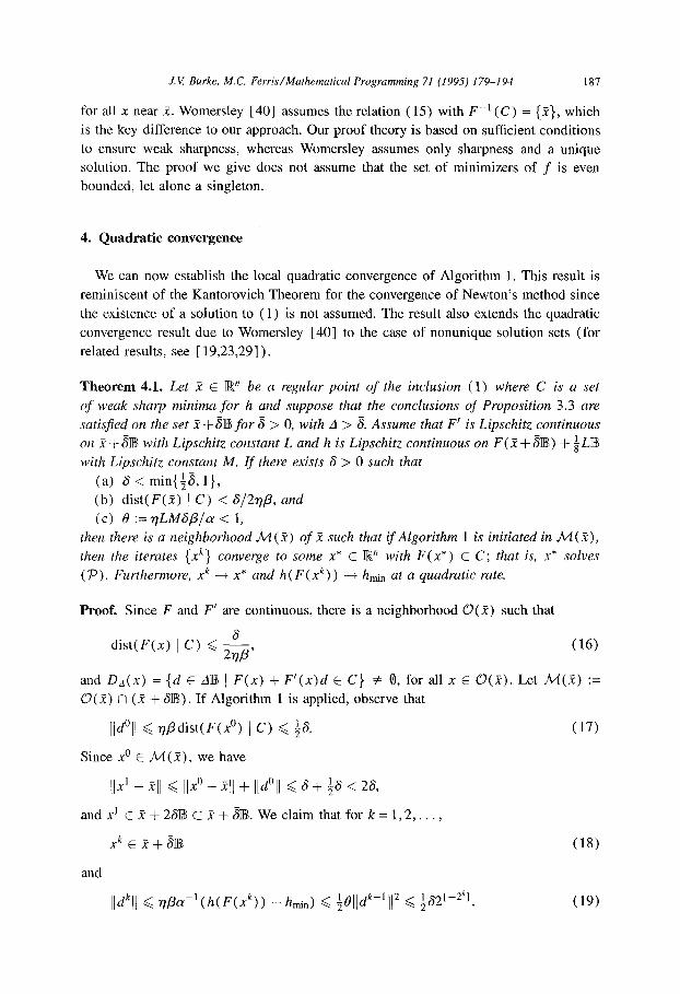
4. Quadratic convergence

We can now establish the local quadratic convergence of Algorithm 1. This result is reminiscent of the Kantorovich Theorem for the convergence of Newton's method since the existence of a solution to (1) is not assumed. The result also extends the quadratic convergence result due to Womersley [40] to the case of nonunique solution sets (for related results, see [ 19,23,29] ).

Theorem 4.1. Let 2 E R" be a regular point o f the inclusion (1) where C is a set

o f weak sharp minima fo r h and suppose that the conclusions of Proposition 3.3 are

satisfied on the set 2 + 6B fo r 6 > O, with A > ~. Assume that F t is Lipschitz continuous on 2 + 6~ with Lipschitz constant L and h is Lipschitz continuous on F ( 2 + ~ ) + ½ L ~

with Lipschitz constant M. I f there exists 6 > 0 such that

(a) 6 < min{½6, 1},

(b) d i s t ( f ( 2 ) I C) < 6/2~7fl, and (c) 0 := rlLM6fl/cr < 1,

then there is a neighborhood 31l(2) of 2 such that if Algorithm 1 is initiated in .Ad( 2), then the iterates {x k} converge to some x* E R '~ with F (x* ) E C; that is, x* solves

(79). Furthermore, x k --+ x* and h ( F ( x k ) ) --+ hn~n at a quadratic rate.

Proof. Since F and F' are continuous, there is a neighborhood 0 ( 2 ) such that

8 d is t (F(x) I C) <~ 2~7-fl' (16)

and DA(X) = {d ~ AB I F ( x ) + F ' ( x ) d ~ C} 4= O, for all x E 0 ( 2 ) . Let .A4(2) := (.9(2) N (2 + 6B). If Algorithm 1 is applied, observe that

IId°ll <~ r l f ld i s t (F(x°) I C) <. ½6. (17)

Since x ° C .A4(2), we have

IIx ~ - 211 ~< II x° - 21[ + [Id°ll ~< 6 + ½6 < 26,

andx j C 2 + 2 6 ~ C 2 + ~ . W e c l a i m t h a t f o r k = 1 , 2 . . . . .

x k E 2 + 6 ~ (18)

and

]]dkll <. ~T f l a - l ( h (F (xk ) ) -hmin) ~< ½0[[dk-lll 2 <<. 162 I-2kl. (19)


Note that (18) implies that the algorithm is well-defined for k = 0, 1,2 . . . . . The proof of the claim proceeds by induction on k.

Observe that (18) has already been established for k = 1. To see (19) for k = 1, first recall that by the quadratic bound lemma [28, 3.2.12]

[[F(x °) + F'(x°)d ° - F(x l ) [ I ~< ½Zlld°ll 2 ~< ~Z,

so that F(x °) + F' (x°)d ° c F(2 + 3~) + ~L~. Thus,

( /o' ) h(F(x l ) ) =h F(x ° ) + F ~ ( x ° ) d ° + (F~(x°+td ° ) - F ~ ( x ° ) ) d ° d t

fo 1 dt <<. h (F(x °) + Fl(x°)d °) + M (F~(x ° + td °) - F~(x °) )d o

fo I dt = hmin + M (F~(x ° + td °) - F~(xO))d °

hmin -]- ½LMIId°II 2, (20)

the second equality following from (12). We now have

IIdlll <.~lflce-l(h(F(xl)) - hmin) (from (4), (11) and (5 ) )

~< ½0Ha°l[ 2 (from (20))

1 I 2 70(~5) (from (17) )

~< ½62 -2.

Next assume that (18) and (19) hold for k = 1 . . . . . s. We show that they also hold

for k = s + 1. First of all, since x ° E .AA(.~), we have

_ 1 ~ 2 - 2 k llxS+l-~ll~<llx° ~11+ tld~tl~<~+½~-~'2E-2~J~<~+~ ~ ' <23, k=0 k=0 k=0

so that x s+l C ~ + ~B. Therefore, as in (20) , h(F(xS+l) ) <~ hmin + ½tMIIdsll 2, and so by the induction hypothesis we obtain

tldS+~ll<~rlflce-l(h(F(x~+~)) - hm~n)<~½OlldSll2<~½0(12~2-2.2) ~< 7321 [-2 s*l ] ,

which concludes our induction. Therefore, the sequence is Cauchy, and so must converge to some x* satisfying

h(F(x*)) = hmin. TO prove the quadratic rate of convergence for {xk), we note from the triangle inequality that

i--I oo

II x~+/- xk+l II ~< ~ llx ~+j+l - xk+Jll ~< ~ It x~+j+l - x~+Jll. j=l j=l

J.E Burke, M.C. Ferris/Mathematical Programming 71 (1995) 179-194 189

For large k, IIx ~+1 - x k l l = • < 1 / (30) . It follows from (19) that II xk÷2 -x~+lll ~< 0• 2, and in general that II x~+j+l -x~+Jt[ <. 02i-x• 2j ~< (o•)J•. Thus, Ilx k+i - x k+l [[ 0 • 2 / ( 1 -- 0 • ), and hence II xk+i - - xk II 2 >/•2 ( ( 1 - 20•) / ( 1 - 0•) ) 2. From these estimates,

llx k÷l - xk+ill 0•2/(1 - 0•) ~< < 60, IIx k - xk+ill 2 • 2 ( ( l -- 2 0 • ) / ( 1 -- 0 • ) ) 2

and the quadratic rate for {x k} follows. The quadratic rate of convergence for { h ( F ( x ~) ) } is obvious from (19) . []

Observe that the above result can also be viewed as a domain of attraction result by assuming that point 2 referred to in the hypotheses actually solves the inclusion (1) . In this case the inequality in assumption (b) is trivially satisfied so that a ~ > 0 satisfying assumptions ( a ) - ( c ) is guaranteed to exist.

5. A globalization strategy

In this section, we propose a globalization strategy for Algorithm 1, based on a backtracking line-search. The algorithm is simply stated as follows.

Algor i thm 2. Let ~7 >~ 1, A E ( 0 , + o c ] , c C (0 ,1 ) , y E (0 ,1 ) and x ° C R" be given. Having x k, determine x k+l as follows.

(1) I f h ( F ( x ) ) = m i n { h ( F ( x ) + U ( x ) d ) I [[dl] ~< A}, then stop; otherwise, choose d k ~ D a ( x k) to satisfy fldkll ~< r/dist(0 I D a ( x k ) ) .

(2) Set x k+l := Xk+ tkd k where tk is the maximum value of ys, for s = 0, 1 . . . . . such

that

h( F ( x ~ + ySdk) ) -- h( F(xk) ) <. cyS[ h( F ( x ~) + F~(xk)d k) - h( F(xk) ) ].

Algorithm 2 is an instance of the class of algorithms studied in [6], so the global convergence properties of the method follow from [6, Theorems 2.4 and 5.3]. These theorems specify the behavior of sequences generated by Algorithm 2 in terms of the first-order optimality conditions for the problem (7)). Recall that a point 2 is a first-order stationary point for the problem (7) ) if

f ' ( 2 ; d ) >/O, for all d E R", (21)

where f t (2; .) (the usual directional derivative of f at the point 2) exists and is finite- valued on R n. By [6, Lemma 4.5 and Theorem 3.6], condition (21) is equivalent to

the condition

h( F( 2) + F' ( Yc)d) - h( F( 2) ) = O,

which can be more simply stated as

for all d C D a ( 2 ) , (22)

0 C D a ( 2 ) . (23)


Conditions (22) and (23) are particularly important in light of the search direction and step-length choice specified in Algorithm 2.

The key global properties for Algorithm 2, established in [6], are stated as the following theorem.

Theorem 5.1. Let x ° E •n and let f = h o F be as in (79). Suppose that F ~ is uniformly

continuous on the closed convex hull o f the set {x E •n: f ( x ) <~ f ( x ° ) } and that h

is Lipschitz on the set {y E Rm: h ( y ) ~ f (x° )} . I f {x k} is the sequence generated by

Algorithm 2 with initial point x °, then at least one o f the following must occur.

(i) The iterates terminate finitely at a first-order stationary point f o r the problem (79).

(ii) The sequence o f values {f(x~)} decreases to - ~ .

(iii) The sequence {lldkll} diverges to .÷~ . (iv) For every subsequence K C {1,2 . . . . ) for which the search directions {dk}K

remain bounded, one has

lim[ h( F( x k) -4- F' ( x k ) d k) - h( F( x k) )] = 0. kEK

Moreover every cluster point o f the subsequence {Xk}K is a first-order stationary point

f o r (79).

An immediate consequence of the above result is that if the set C = argmin h is nonempty and A < + ~ , then

lim[ h( F( x k) -4- F' ( x k ) d k) - h( F( xk) ) ] = O, k

and every cluster point of the sequence {x k} is a first-order stationary point for (79). We now further analyze the convergence behavior at cluster points satisfying the sharpness and regularity hypotheses.

Theorem 5.2. Let f := h o F be as in (79) with h finite-valued and F ~ locally Lipschitz

continuous. Suppose that {x k} is a sequence generated by Algorithm 2 and that Yc is a

cluster point o f this sequence. I f 2 is a regular point o f the inclusion ( 1 ) where C is a

set o f weak sharp minima fo r h, then F(Yc) ~ C and both x k --~ Y: and f ( x k) --+ hmin at a quadratic rate.

Proof. We first show that F ( 2 ) E C. By Theorem 5.1, we have 0 C U(Yc)T3h(F(Yc)) .

If F ( 2 ) ~ C, then 0 ¢ O h ( F ( 2 ) ) in which case there is a nonzero z E Oh(F(2 ) ) N kerU(5:) v. But z C F c ( F( 2 ) ) since 0 ~> h ( y ) - h( F( 2) ) >~ (z, y - F( 2) ), for all y C C, so that

z C {v: ( v , F ( Y c ) ) - ~ c ( v ) > ~ 0 } = r c ( F ( ~ ) ) (by (8)) .

This contradicts the assumption that ~ is a regular point of the inclusion (1), hence F(.~) ~ C.

J. ~ Burke, M.C. Ferris/Mathematical Programming 71 (1995) 179-194 191

We now establish the convergence rates. Since the regularity hypothesis at 2 implies

that F ( 2 ) C C, the result will follow immediately from Theorem 4.1 if it can be shown that there is a neighborhood N of 2 such that

h ( F ( x ÷ d) ) - h ( F ( x ) ) <~ c [ h ( F ( x ) + F ' ( x ) d ) - h ( F ( x ) ) ], (24)

for all x E N and d E R n satisfying ]]dl[ ~< 7/dist(0 I D,a(x)) . Indeed, if (24) holds,

then Algorithms 1 and 2 generate identical iterates sufficiently close to 2. Hence, by Theorem 4.1, these iterates remain close to 2 and converge to a solution of (79). Since )~

is a cluster point of this sequence, the entire sequence must converge to 2 with x k ~

and f ( x ~) --+ hmin quadratically. Suppose to the contrary that (24) does not hold near 2. Then there is a sequence

{2 k } converging to 2 such that

c [ h ( F ( 2 k) + U ( 2 k ) d k) - h ( f ( 2 k ) ) ] < h ( F ( 2 k + d ~ ) ) - h ( F ( 2 k ) ) (25)

at each 2 k for some d ~ C R n satisfying

Ildkll <~ Bdist(0 I D,a(2k)). (26)

In particular, we obtain from (11) that

Ildkll -+ 0. (271

Let N1 be a compact neighborhood of 2 containing the set 2 + 2AII~ and let K and M be Lipschitz constants for h on F (N1) and U on N1, respectively. Let A > 8 > 0 be

chosen so that the conclusions of Proposition 3.3 hold for this choice of 6. We suppose

with no loss of generality that {2 k} C 2 + 8 ~ . Then for all k we have from [28, 3.2.12]

that

h(F(Y: k + dk)) - hmin = Ilh(F(2 k + dk)) - h ( F ( 2 k) + F ' ( 2 k ) d ~) II

<. KIIF(Yc k + d g) - F(2 k) - F'(2t)dkl l

<<. ½gMIIdk[[ 2.

Therefore, by (25),

c[hmin - h( F( 2 k) ) ] = c[ h( F( 2 k) + F' ( 2k)d k) - h( F( Yc k) ) ]

< h ( F ( 2 k + dk)) - h (F(2~) )

<~ h ~ . - h ( F ( ~ k ) t + ½KMl[dkll 2.

Consequently,

0 < (1 - c) [hmin - h(F(yck))] q- ½KMlldkt[ 2

<<. (C -- 1 ) a d i s t ( F ( 2 k) I C) + ½gMIIdkll 2 (from (511

~< (c - l )a ( /3n) - l l ldk l ] + ½gMlldkll 2 (from (11) and (26) ) .


After dividing this expression through by ]ldkll and using (27) while taking the limit in k, we obtain the contradiction 0 ~< (c - l ) a ( /3 r / ) -1. []

6. Concluding remarks

We have shown that under the assumptions of weak sharpness and regularity one obtains the local quadratic convergence of a Gauss-Newton method for convex composite optimization. Moreover, the method can be "globalized" with the addition of a backtracking line-search that does not inhibit the local rate. A similar result can be established for a trust-region-based globalization strategy.

Let us briefly consider the implications for the case of the nonlinear least squares (NLLS) . Consider Algorithm 1 under the assumptions of weak sharpness and regularity. Recall that the regularity condition implies that i m ( U ( x ) ) = ~m so that n ~> m. This instance of the NLLS problem seems to have received little study [13,15,28]. Nonetheless, it is of great significance in the description of constraint regions in nonlinear programming. In this case, condition (4) with r / = 1 in Algorithm 1 is easily satisfied with the aid of either a QR factorization or a singular-value decomposition. In either case, the algorithm is locally equivalent to the Ben-Israel iteration for NLLS [1,3]. In their analyses of this iteration, neither Ben-Israel [ 1 ] or Boggs [3] establish a rate of convergence for the method nor do they provide a globalization strategy. The results of this article can be applied to fill in these gaps.

In the context of solving the more general problem (1) , recall that near a regular

solution to this inclusion, the direction-finding subproblem in Algorithm 1 corresponds to locating a least-norm solution to the linearized problem F ( x k) ÷ U ( x k ) d = O.

Thus, the method is locally equivalent to the procedure described in [23], It is also

equivalent to the procedure given in [33] if C is a cone. Robinson [33] ( i f C is a cone) and Maguregui [23] obtain a Kantorovich-type convergence result. Theorem 4.1 is similar to these results since it can also be viewed as an existence result for the inclusion (1). Robinson's approach appeals to the theory of normed convex processes [34] , while Maguregui makes use of the Robinson-Ursescu Theorem [36] along with the perturbation theory in [22]. The proof theory provided in this article is more elementary and accessible since it only requires a straightforward application of Fenchel duality. Moreover, we improve the applicability of the theory by providing a simple globalization strategy that preserves the local rate.

References

[I ] A. Ben-Israel, "A Newton-Raphson method for the solution of systems of equations," Journal of Mathematical Analysis and its Applications 15 (1966) 243-252.

[21 S.C. Billups and M.C. Ferris, "Solutions to affine generalized equations using proximal mappings," Mathematical Programming Technical Report 94-15 (Madison, WI, 1994).

[3] ET. Boggs, "The convergence of the Ben-Israel iteration for nonlinear least squares problems," Mathematics of Computation 30 (1976) 512-522.

J. ~ Burke, M.C. Ferris/Mathematical Programming 71 (1995) 179-194 193

[4] J.M. Borwein, "Stability and regular points of inequality systems" Journal of Optimization Theory and Applications 48 (1986) 9-52.

[5 L J.V. Burke, "Algorithms for solving finite dimensional systems of nonlinear equations and inequalities that have both global and quadratic convergence properties," Report ANL/MCS-TM-54, Mathematics and Computer Science Division, Argonne National Laboratory (Argonne, IL, 1985).

[6] J.V. Burke, "Descent methods for composite nondifferentiable optimization problems," Mathematical Programming 33 (3) (1985) 260-279.

[7] J.V. Burke, "An exact penalization viewpoint of constrained optimization," SIAM Journal on Control and Optimization 29 (1991) 968-998.

[8] J.V. Burke and M.C. Ferris, "Weak sharp minima in mathematical programming," SIAM Journal on Control and Optimization 31 (1993) 1340-1359.

19] J.V. Burke and R.A. Poliquin, "Optimality conditions for non-finite valued convex composite functions" Mathematical Programming 57 (1) (1992) 103-120.

[ 10] J.V. Burke and E Tseng, "A unified analysis of Hoffman's bound via Fenchel duality," SIAM Journal on Optimization, to appear.

[ 11 ] L. Cromme, "Strong uniqueness. A far reaching criterion for the convergence analysis of iterative procedures" Numerische Mathematik 29 (1978) 179-193.

[ 12] R. De Leone and O.L. Mangasarian, "Serial and parallel solution of large scale linear programs by augmented Lagrangian successive overrelaxation" in: A. Kurzhanski et al., eds., Optimization, Parallel Processing and Applications, Lecture Notes in Economics and Mathematical Systems, Vol. 304 (Springer, Berlin, 1988) pp. 103-124.

[ 13] J.E. Dennis and R.B. Schnabel, Numerical Methods for Unconstrained Optimizations and Nonlinear Equations (Prentice-Hall, Englewood Cliffs, NJ, 1983).

[ 14] M.C. Ferris, "Weak sharp minima and penalty functions in mathematical programming," Ph.D. Thesis, University of Cambridge (Cambridge, 1988).

[15 ] R. Fletcher, "Generalized inverse methods for the best least squares solution of non-linear equations," The Computer Journal 10 (1968) 392-399.

[ 16] R. Fletcher, "Second order correction for nondifferentiable optimization" in: G.A. Watson, ed., Numerical Analysis, Lecture Notes in Mathematics, Vol. 912 (Springer, Berlin, 1982) pp. 85-114.

[ 171 R. Fletcher, Practical Methods of Optimization (Wiley, New York, 2nd ed., 1987). [ 18] U.M. Garcia-Palomares and A. Restuccia, "A global quadratic algorithm for solving a system of mixed

equalities and inequalities," Mathematical Programming 21 (3) ( 1981 ) 290-300. [ 19 ] K. Jittorntrum and M.R. Osborne, "Strong uniqueness and second order convergence in nonlinear discrete

approximation" Numerische Mathematik 34 (1980) 439-455. [20] K. Levenberg, "A method for the solution of certain nonlinear problems in least squares," Quarterly

Applied Mathematics 2 (1944) 164-168. [ 2 l ] K. Madsen, "Minimization of nonlinear approximation functions," Ph.D. Thesis, Institute of Numerical

Analysis, Technical University of Denmark (Lyngby, 1985). [221 J. Maguregui, "Regular multivalued functions and algorithmic applications," Ph.D. Thesis, University of

Wisconsin (Madison, WI, 1977). [231 J. Maguregui, "A modified Newton algorithm for functions over convex sets" in: O.L. Mangasarian,

R.R. Meyer and S.M. Robinson, eds., Nonlinear Programming 3 (Academic Press, New York, 1978) pp. 461-473.

[241 O.L. Mangasarian, "Least-norm linear programming solution as an unconstrained minimization problem" Journal of Mathematical Analysis and Applications 92 ( 1 ) ( 1983) 240-251.

[25] O.L. Mangasarian, "Normal solutions of linear programs," Mathematical Programming Study 22 (1984) 206 -216.

[126] O.L. Mangasarian and S. Fromovitz, "The Fritz John necessary optimality conditions in the presence of equality and inequality constraints," Journal of Mathematical Analysis and its Applications 17 (1967) 37-47.

12711 D.W. Marquardt, "An algorithm for least-squares estimation of nonlinear parameters," SIAM Journal of Applied Mathematics 11 (1963) 431-441.

[281 J.M. Ortega and W.C. Rheinboldt, lterative Solution of Nonlinear Equations in Several Variables (Academic Press, New York, 1970).

[ 29] M.R. Osborne and R.S. Womersley, "Strong uniqueness in sequential linear programming" Journal of the Australian Mathematical Society. Series B 31 (1990) 379-384,


[301 B.T. Polyak, Introduction to Optimization (Optimization Software, New York, 1987). [31 [ M.J.D. Powell, "General algorithm for discrete nonlinear approximation calculations," in: C.K. Chui,

L.L. Schumaker and J.D. Ward, eds., Approximation Theory IV (Academic Press, New York, 1983) pp. 187-218.

[32] H. Rhdstrthn, "An embedding theorem for spaces of convex sets," Proceedings of the American Mathematical Society 3 (1952) 165-169.

[33] S.M. Robinson, "Extension of Newton's method to nonlinear functions with values in a cone," Numerische Mathematik 19 (1972) 341-347.

[ 34] S.M. Robinson, "Normed convex processes," Transactions of the American Mathematical Society 174 (1972) 127-140.

[135[ S. Robinson, "Stability theory for systems of inequalities, Part I: linear systems," SIAM Journal on Numerical Analysis 12 (1975) 754-769.

[36] S. Robinson, "Regularity and stability for convex multivalued functions," Mathematics of Operations Research 1 (1976) 130-143.

[37] S. Robinson, "Stability theory for systems of inequalities, Part II: Differentiable nonlinear systems," SlAM Journal on Numerical Analysis 13 (1976) 497-513.

[381] R.T. Rockafellar, Convex Analysis (Princeton University Press, Princeton, NJ, 1970). [39] R.T. Rockafellar, "First- and second-order epi-differentiability in nonlinear programming," Transactions

of the American Mathematical Society 307 (1988) 75-108. [40] R.S. Womersley, "Local properties of algorithms for minimizing nonsmooth composite functions,"

Mathematical Programming 32 ( 1 ) (1985) 69-89.

A Gauss—Newton method for convex composite...

Documents

Transcript of A Gauss—Newton method for convex composite...