A Gauss–Newton Approach for Solving Constrained ...andreani/papers/anfusi.pdf · J Optim Theory...
33
J Optim Theory Appl (2013) 156:417–449 DOI 10.1007/s10957-012-0114-6 A Gauss–Newton Approach for Solving Constrained Optimization Problems Using Differentiable Exact Penalties Roberto Andreani · Ellen H. Fukuda · Paulo J.S. Silva Received: 1 June 2012 / Accepted: 16 June 2012 / Published online: 29 June 2012 © Springer Science+Business Media, LLC 2012 Abstract We propose a Gauss–Newton-type method for nonlinear constrained opti- mization using the exact penalty introduced recently by André and Silva for varia- tional inequalities. We extend their penalty function to both equality and inequality constraints using a weak regularity assumption, and as a result, we obtain a continu- ously differentiable exact penalty function and a new reformulation of the KKT con- ditions as a system of equations. Such reformulation allows the use of a semismooth Newton method, so that local superlinear convergence rate can be proved under an assumption weaker than the usual strong second-order sufficient condition and with- out requiring strict complementarity. Besides, we note that the exact penalty function can be used to globalize the method. We conclude with some numerical experiments using the collection of test problems CUTE. Keywords Exact penalty · Multipliers estimate · Nonlinear programming · Semismooth Newton method Communicated by Gianni Di Pillo. R. Andreani · E.H. Fukuda Department of Applied Mathematics, IMECC, State University of Campinas, Campinas, Brazil R. Andreani e-mail: [email protected] E.H. Fukuda e-mail: [email protected] P.J.S. Silva ( ) Department of Computer Science, IME, University of São Paulo, São Paulo, Brazil e-mail: [email protected]
-
Upload
nguyennguyet -
Category
Documents
-
view
215 -
download
0
Transcript of A Gauss–Newton Approach for Solving Constrained ...andreani/papers/anfusi.pdf · J Optim Theory...
J Optim Theory Appl (2013) 156:417–449DOI 10.1007/s10957-012-0114-6
A Gauss–Newton Approach for Solving ConstrainedOptimization Problems Using Differentiable ExactPenalties
Roberto Andreani · Ellen H. Fukuda ·Paulo J.S. Silva
Received: 1 June 2012 / Accepted: 16 June 2012 / Published online: 29 June 2012© Springer Science+Business Media, LLC 2012
Abstract We propose a Gauss–Newton-type method for nonlinear constrained opti-mization using the exact penalty introduced recently by André and Silva for varia-tional inequalities. We extend their penalty function to both equality and inequalityconstraints using a weak regularity assumption, and as a result, we obtain a continu-ously differentiable exact penalty function and a new reformulation of the KKT con-ditions as a system of equations. Such reformulation allows the use of a semismoothNewton method, so that local superlinear convergence rate can be proved under anassumption weaker than the usual strong second-order sufficient condition and with-out requiring strict complementarity. Besides, we note that the exact penalty functioncan be used to globalize the method. We conclude with some numerical experimentsusing the collection of test problems CUTE.
Keywords Exact penalty · Multipliers estimate · Nonlinear programming ·Semismooth Newton method
Communicated by Gianni Di Pillo.
R. Andreani · E.H. FukudaDepartment of Applied Mathematics, IMECC, State University of Campinas, Campinas, Brazil
R. Andreanie-mail: [email protected]
E.H. Fukudae-mail: [email protected]
P.J.S. Silva (�)Department of Computer Science, IME, University of São Paulo, São Paulo, Brazile-mail: [email protected]
418 J Optim Theory Appl (2013) 156:417–449
1 Introduction
A popular framework to solve constrained nonlinear programming problems is to usepenalty-based methods, such as quadratic penalty functions, augmented Lagrangiansand exact penalty functions. The last one consists in replacing the original constrainedproblem with a single unconstrained one. Recently, André and Silva [1] proposed anexact penalty function for variational inequalities. Their idea is based on Di Pilloand Grippo’s work [2, 3], which consists in incorporating a multipliers estimate in anaugmented Lagrangian function. In this work, we propose a modified multipliers esti-mate and extend the exact penalty function for variational inequalities to optimizationproblems with general equality and inequality constraints. We use a generalized New-ton method to solve the associated reformulation of the KKT conditions and define asuitable merit function to globalize the method.
The paper is organized as follows. In Sect. 2, we give some notations, definitionsand the background concerning exact penalty functions. In Sect. 3, we construct theexact penalty function and present some results associated to the modified multipli-ers estimate. Exactness results are presented in Sect. 4, and in Sect. 5 we show away to dynamically update the penalty parameter. Local convergence results for thesemismooth Newton method are presented in Sect. 6. We finish in Sect. 7, with aglobalization idea and some numerical experiments.
2 Preliminaries
Consider the following nonlinear programming problem:
min f (x) s.t. x ∈ X, (NLP)
where the feasible set is assumed to be nonempty and is defined by
X := {x ∈ R
n : h(x) = 0, g(x) ≤ 0},
and f : Rn → R, g : R
n → Rm and h : R
n → Rp are C 2 functions. Roughly speak-
ing, a function wc : Rn → R, that depends on a positive parameter c ∈ R, is an exact
penalty function for the problem (NLP) if there is an appropriate choice of the penaltycoefficient c such that a single minimization of wc recovers a solution of (NLP).
A well-known exact penalty function is the one proposed by Zangwill [4]. It canbe shown that the solutions of the constrained problem (NLP) are solutions of thefollowing unconstrained one:
minx
[f (x) + c max
{0, g1(x), . . . , gm(x),
∣∣h1(x)∣∣, . . . ,
∣∣hp(x)∣∣}],
under reasonable conditions and when c is sufficiently large [5, Sect. 4.3.1]. However,the maximum function contained in such penalty function makes it nondifferentiable,which demands special methods to solve this unconstrained problem. Besides, it isnot easy to find the value of the parameter c that ensures the recovering of solutionsof (NLP).
J Optim Theory Appl (2013) 156:417–449 419
To overcome such difficulty, many authors proposed continuously differentiableexact penalty functions. The first ones were introduced by Fletcher [6] and by Gladand Polak [7], respectively, for problems with equality constraints and for those withboth equality and inequality constraints. Another important contribution was done byMukai and Polak [8]. In problems associated to such penalties, the variables are in thesame space as the variables of the original problem. An alternative approach consistsin defining an unconstrained minimization problem on the product space of variablesand multipliers. This last case, called exact augmented Lagrangian methods, wasintroduced later by Di Pillo and Grippo [9, 10].
Considering only problems with equality constraints, these authors formulated theunconstrained problem as follows:
minx,μ
[f (x) + ⟨
μ,h(x)⟩ + c
2
∥∥h(x)∥∥2 + 1
2
∥∥M(x)(∇f (x) + Jh(x)T μ
)∥∥2],
where 〈·, ·〉 and ‖·‖ denote the Euclidean inner product and norm, respectively, Jh(x)
is the Jacobian of h at x and M(x) ∈ R�×n is a C 2 matrix with p ≤ � ≤ n and such
that M(x)Jh(x)T has full rank. Suitable choices of M(x) make the above objectivefunction quadratic in the dual variable μ. In such a case, we can write the multiplierin terms of x and incorporate it again in the function, obtaining an unconstrainedproblem in the space of the original variables. Some of the choices of M(x) recoverthe exact penalties of Fletcher and Mukai and Polak.
For problems with inequality constraints, we can add slack variables and write itin terms of x using an appropriate choice of matrix M(x). Nevertheless, it is notknown a formula for M(x) that also isolates the multiplier. After this, Di Pillo andGrippo proposed a new continuously differentiable exact penalty, this time takingGlad and Polak’s multipliers estimate [7] as a base. The idea was presented in [11]and [3] and it consists in constructing an exact penalty function by incorporating suchestimate in the augmented Lagrangian of Hestenes, Powell, and Rockafellar [12–14].To overcome some theoretical limitations of such penalty, Lucidi proposed in [15]another exact penalty function for problems with inequality constraints.
The same idea was extended recently by André and Silva [1] to solve variationalinequalities with the feasible set defined by functional inequality constraints. In theirwork, they incorporated Glad and Polak’s multipliers estimate in the augmented La-grangian for variational inequalities, proposed by Auslender and Teboulle [16]. If thevariational problem comes from the first-order necessary condition of an optimiza-tion problem, then this penalty is equivalent to the gradient of Di Pillo and Grippo’spenalty excluding second-order terms. This is important from the numerical point ofview, because otherwise it would be necessary to deal with third-order terms whensecond-order methods, like the Newton method, are applied to solve the problem. Inthe optimization case, Newton-type methods based on exact merit functions (exactpenalties and exact augmented Lagrangians), without the knowledge of third-orderterms, have been also proposed [17–20]. In particular, an exact penalty function wasused in [17] for problems with equality constraints.
In this work, we extend André and Silva’s exact penalty to solve optimizationproblems like (NLP), that is, with both equality and inequality constraints. We also
420 J Optim Theory Appl (2013) 156:417–449
adapt Glad and Polak’s multipliers estimate in order to use a weaker regularity as-sumption and compare it with the one proposed by Lucidi in [15]. The obtained func-tion is semismooth or, under some conditions, strongly semismooth, which allowsthe use of the semismooth Newton method to solve the associated system of equa-tions [21]. Exactness results are established and we adapt some results of Facchinei,Kanzow, and Palagi [22] to prove that the convergence rate is superlinear (or, in somecases, quadratic) without requiring strict complementarity or strong second-order suf-ficient condition. Moreover, we indicate a way to globalize the method using a spe-cific merit function that makes it works as a Gauss–Newton-type method.
3 Constructing the Exact Penalty
The construction of the exact penalty function is based on Di Pillo and Grippo’s [3,11] and André and Silva’s [1] papers. In both cases, the authors incorporate a La-grange multipliers estimate in an augmented Lagrangian function. In particular, theyboth use the estimate proposed by Glad and Polak [7], which requires that the gradi-ents of active inequality constraints ∇gi(x), i ∈ {i : gi(x) = 0} and all the gradientsof equality constraints ∇hi(x), i = 1, . . . , p are linearly independent for all x ∈ R
n.This condition is called linear independence constraint qualification (LICQ) and, inthe optimization literature, is usually referred only at feasible points of the problem.
However, methods based on exact penalties may need to compute multipliers es-timates in infeasible points, and hence LICQ has to be assumed to hold in the wholespace R
n. Thus, it is interesting to search for estimates that depend on a weaker as-sumption than LICQ in R
n. With this in mind, we introduce the following condition.
Definition 3.1 A point x ∈ Rn satisfies the relaxed linear independence constraint
qualification (relaxed LICQ) or, equivalently, it is called regular, if and only if thegradients
∇gi(x), i ∈ I=(x), ∇hi(x), i ∈ E=(x)
are linearly independent, where
I=(x) := {i ∈ {1, . . . ,m} : gi(x) = 0
}and E=(x) := {
i ∈ {1, . . . , p} : hi(x) = 0}.
Also, define the set of regular points in Rn as1
R := {x ∈ R
n : x satisfies relaxed LICQ}.
This condition is more reasonable than LICQ because it allows more infeasiblepoints to satisfy it. To illustrate such advantage, consider n = 2, m = 2, p = 1, andfunctions defined by g1(x) := −x1 +x2, g2(x) := x1 +x2 −1 and h1(x) := x2. Takingthe infeasible point x := (0.5,0.5)T , we observe that I=(x) = {1,2} and E=(x) = ∅.Therefore, x satisfies relaxed LICQ, but not LICQ.
1The notation R comes from the word regularity.
J Optim Theory Appl (2013) 156:417–449 421
By replacing LICQ with relaxed LICQ, we can adapt Glad and Polak’s multipliersestimate. In this case, we obtain the estimate by solving the following unconstrainedminimization problem, with variables λ ∈ R
m and μ ∈ Rp associated to inequality
and equality constraints, respectively:
minλ,μ
∥∥∇xL(x,λ,μ)∥∥2 + ζ 2(∥∥G(x)λ
∥∥2 + ∥∥H(x)μ∥∥2)
, (1)
where L(x,λ,μ) := f (x) + 〈λ,g(x)〉 + 〈μ,h(x)〉 is the Lagrangian function, ζ > 0,G(x) := diag(g1(x), . . . , gm(x)) and H(x) := diag(h1(x), . . . , hp(x)) are diagonalmatrices with diagonal entries gi(x), i = 1, . . . ,m and hi(x), i = 1, . . . , p, respec-tively.
Considering the KKT conditions of (NLP), we observe that the above minimiza-tion problem forces the zero condition ∇xL(x,λ,μ) = 0 and the complementaryslackness 〈g(x), λ〉 = 0. This also happens in Glad and Polak’s estimate. The differ-ence is that the new one adds the term ‖H(x)μ‖2. Thus, it also enforces the com-plementarity of equality constraints 〈h(x),μ〉 = 0, even if it is irrelevant in the KKTconditions. The interesting fact is that this new estimate allows the use of the weakerassumption, the relaxed LICQ, and it does not lose any properties of Glad and Polak’sestimate. In fact, the associated problem (1) is equivalent to
minλ,μ
∥∥∥∥∥∥
⎡
⎣Jg(x)T Jh(x)T
ζG(x) 00 ζH(x)
⎤
⎦[
λ
μ
]−
⎡
⎣−∇f (x)
00
⎤
⎦
∥∥∥∥∥∥
2
, (2)
that is, it is a linear least squares problem. The proposition below gives some otherproperties associated to the modified multipliers estimate.
Proposition 3.1 Assume that x ∈ Rn satisfies the relaxed LICQ and define the matrix
N(x) ∈ R(m+p)×(m+p) by
N(x) :=[Jg(x)Jg(x)T + ζ 2G(x)2 Jg(x)Jh(x)T
Jh(x)Jg(x)T Jh(x)Jh(x)T + ζ 2H(x)2
].
Then
(a) The matrix N(x) is positive definite.(b) The solution of (1) (equivalently, (2)) is unique and it is given by
[λ(x)
μ(x)
]= −N−1(x)
[Jg(x)
Jh(x)
]∇f (x).
(c) If (x, λ, μ) ∈ Rn+m+p satisfies the KKT conditions, then λ = λ(x) and μ = μ(x).
(d) The Jacobian matrices of λ(·) and μ(·) are given by
[Jλ(x)
Jμ(x)
]= −N−1(x)
[R1(x)
R2(x)
],
422 J Optim Theory Appl (2013) 156:417–449
with
R1(x) := Jg(x)∇2xxL
(x,λ(x),μ(x)
) + 2ζ 2Λ(x)G(x)Jg(x)
+m∑
i=1
emi ∇xL
(x,λ(x),μ(x)
)T ∇2gi(x),
R2(x) := Jh(x)∇2xxL
(x,λ(x),μ(x)
) + 2ζ 2M(x)H(x)Jh(x)
+p∑
i=1
epi ∇xL
(x,λ(x),μ(x)
)T ∇2hi(x),
where Λ(x) := diag(λ1(x), . . . , λm(x)) and M(x) := diag(μ1(x), . . . ,μp(x))
are diagonal matrices respectively with elements λi(x) := [λ(x)]i and μi(x) :=[μ(x)]i , em
i , epi are the i-th elements of the canonical base of R
m and Rp , re-
spectively, and
∇xL(x,λ(x),μ(x)
) := ∇xL(x,λ,μ)|λ=λ(x),μ=μ(x),
∇2xxL
(x,λ(x),μ(x)
) := ∇2xxL(x,λ,μ)|λ=λ(x),μ=μ(x).
Proof (a) Let A(x) ∈ R(n+m+p)×(m+p) be the matrix associated to the linear least
squares problem (2), that is,
A(x) :=⎡
⎣Jg(x)T Jh(x)T
ζG(x) 00 ζH(x)
⎤
⎦ . (3)
Without loss of generality, we can write Jg(x)T = [Jg(x)T= |Jg(x)T=], where Jg(x)=and Jg(x)= correspond to the parts of Jg(x) where gi(x) = 0 and gi(x) = 0, respec-tively. In the same way, we can define the matrices Jh(x)=, Jh(x)=, G(x)= andH(x)=. Thus,
A(x) =
⎡
⎢⎢⎢⎢⎣
Jg(x)T= Jg(x)T= Jh(x)T= Jh(x)T=0 0 0 00 ζG(x)= 0 00 0 0 00 0 0 ζH(x)=
⎤
⎥⎥⎥⎥⎦
,
and we can see that it has linearly independent columns, by relaxed LICQ (so thefirst and third block columns of A(x) are linearly independent) and because of thenonzero block diagonal matrices G(x)= and H(x)=. Furthermore, it is easy to seethat N(x) = A(x)T A(x), so we can conclude that N(x) is nonsingular and positivedefinite.
J Optim Theory Appl (2013) 156:417–449 423
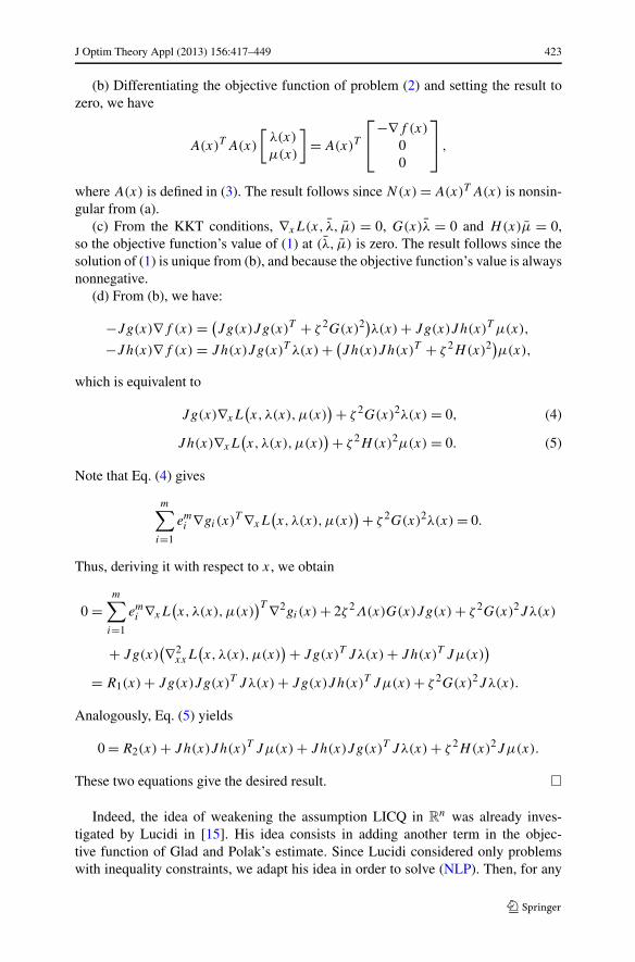
(b) Differentiating the objective function of problem (2) and setting the result tozero, we have
A(x)T A(x)
[λ(x)
μ(x)
]= A(x)T
⎡
⎣−∇f (x)
00
⎤
⎦ ,
where A(x) is defined in (3). The result follows since N(x) = A(x)T A(x) is nonsin-gular from (a).
(c) From the KKT conditions, ∇xL(x, λ, μ) = 0, G(x)λ = 0 and H(x)μ = 0,so the objective function’s value of (1) at (λ, μ) is zero. The result follows since thesolution of (1) is unique from (b), and because the objective function’s value is alwaysnonnegative.
(d) From (b), we have:
−Jg(x)∇f (x) = (Jg(x)Jg(x)T + ζ 2G(x)2)λ(x) + Jg(x)Jh(x)T μ(x),
−Jh(x)∇f (x) = Jh(x)Jg(x)T λ(x) + (Jh(x)Jh(x)T + ζ 2H(x)2)μ(x),
which is equivalent to
Jg(x)∇xL(x,λ(x),μ(x)
) + ζ 2G(x)2λ(x) = 0, (4)
Jh(x)∇xL(x,λ(x),μ(x)
) + ζ 2H(x)2μ(x) = 0. (5)
Note that Eq. (4) gives
m∑
i=1
emi ∇gi(x)T ∇xL
(x,λ(x),μ(x)
) + ζ 2G(x)2λ(x) = 0.
Thus, deriving it with respect to x, we obtain
0 =m∑
i=1
emi ∇xL
(x,λ(x),μ(x)
)T ∇2gi(x) + 2ζ 2Λ(x)G(x)Jg(x) + ζ 2G(x)2Jλ(x)
+ Jg(x)(∇2
xxL(x,λ(x),μ(x)
) + Jg(x)T Jλ(x) + Jh(x)T Jμ(x))
= R1(x) + Jg(x)Jg(x)T Jλ(x) + Jg(x)Jh(x)T Jμ(x) + ζ 2G(x)2Jλ(x).
Analogously, Eq. (5) yields
0 = R2(x) + Jh(x)Jh(x)T Jμ(x) + Jh(x)Jg(x)T Jλ(x) + ζ 2H(x)2Jμ(x).
These two equations give the desired result. �
Indeed, the idea of weakening the assumption LICQ in Rn was already inves-
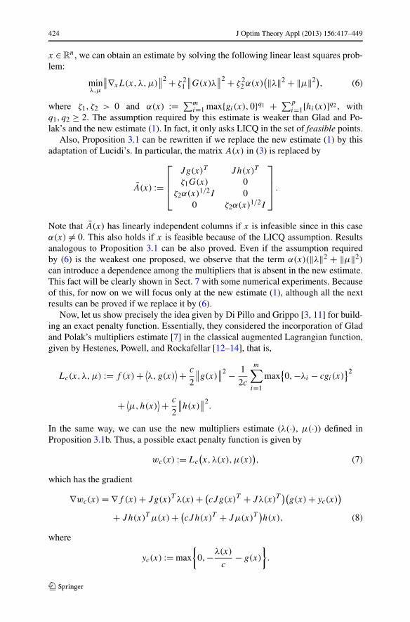
tigated by Lucidi in [15]. His idea consists in adding another term in the objec-tive function of Glad and Polak’s estimate. Since Lucidi considered only problemswith inequality constraints, we adapt his idea in order to solve (NLP). Then, for any
424 J Optim Theory Appl (2013) 156:417–449
x ∈ Rn, we can obtain an estimate by solving the following linear least squares prob-
lem:
minλ,μ
∥∥∇xL(x,λ,μ)∥∥2 + ζ 2
1
∥∥G(x)λ∥∥2 + ζ 2
2 α(x)(‖λ‖2 + ‖μ‖2), (6)
where ζ1, ζ2 > 0 and α(x) := ∑mi=1 max{gi(x),0}q1 + ∑p
i=1[hi(x)]q2 , withq1, q2 ≥ 2. The assumption required by this estimate is weaker than Glad and Po-lak’s and the new estimate (1). In fact, it only asks LICQ in the set of feasible points.
Also, Proposition 3.1 can be rewritten if we replace the new estimate (1) by thisadaptation of Lucidi’s. In particular, the matrix A(x) in (3) is replaced by
A(x) :=
⎡
⎢⎢⎣
Jg(x)T Jh(x)T
ζ1G(x) 0ζ2α(x)1/2I 0
0 ζ2α(x)1/2I
⎤
⎥⎥⎦ .
Note that A(x) has linearly independent columns if x is infeasible since in this caseα(x) = 0. This also holds if x is feasible because of the LICQ assumption. Resultsanalogous to Proposition 3.1 can be also proved. Even if the assumption requiredby (6) is the weakest one proposed, we observe that the term α(x)(‖λ‖2 + ‖μ‖2)
can introduce a dependence among the multipliers that is absent in the new estimate.This fact will be clearly shown in Sect. 7 with some numerical experiments. Becauseof this, for now on we will focus only at the new estimate (1), although all the nextresults can be proved if we replace it by (6).
Now, let us show precisely the idea given by Di Pillo and Grippo [3, 11] for build-ing an exact penalty function. Essentially, they considered the incorporation of Gladand Polak’s multipliers estimate [7] in the classical augmented Lagrangian function,given by Hestenes, Powell, and Rockafellar [12–14], that is,
Lc(x,λ,μ) := f (x) + ⟨λ,g(x)
⟩ + c
2
∥∥g(x)∥∥2 − 1
2c
m∑
i=1
max{0,−λi − cgi(x)
}2
+ ⟨μ,h(x)
⟩ + c
2
∥∥h(x)∥∥2
.
In the same way, we can use the new multipliers estimate (λ(·), μ(·)) defined inProposition 3.1b. Thus, a possible exact penalty function is given by
wc(x) := Lc
(x,λ(x),μ(x)
), (7)
which has the gradient
∇wc(x) = ∇f (x) + Jg(x)T λ(x) + (cJg(x)T + Jλ(x)T
)(g(x) + yc(x)
)
+ Jh(x)T μ(x) + (cJh(x)T + Jμ(x)T
)h(x), (8)
where
yc(x) := max
{0,−λ(x)
c− g(x)
}.
J Optim Theory Appl (2013) 156:417–449 425
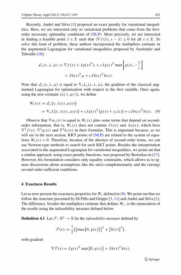
Recently, André and Silva [1] proposed an exact penalty for variational inequal-ities. Here, we are interested only in variational problems that come from the first-order necessary optimality conditions of (NLP). More precisely, we are interestedin finding a feasible point x ∈ X such that 〈∇f (x), x − x〉 ≥ 0 for all x ∈ X. Tosolve this kind of problem, these authors incorporated the multipliers estimate inthe augmented Lagrangian for variational inequalities proposed by Auslender andTeboulle [16]:
Lc(x,λ,μ) := ∇f (x) + Jg(x)T λ + cJg(x)T max
{g(x),−λ
c
}
+ Jh(x)T μ + cJh(x)T h(x).
Note that Lc(x,λ,μ) is equal to ∇xLc(x,λ,μ), the gradient of the classical aug-mented Lagrangian for optimization with respect to the first variable. Once again,using the new estimate (λ(·),μ(·)), we define
Wc(x) := Lc
(x,λ(x),μ(x)
)
= ∇xL(x,λ(x),μ(x)
) + cJg(x)T(g(x) + yc(x)
) + cJh(x)T h(x). (9)
Observe that ∇wc(x) is equal to Wc(x) plus some terms that depend on second-order information, that is, Wc(x) does not contain Jλ(x) and Jμ(x), which have∇2f (x), ∇2gi(x) and ∇2hi(x) in their formulas. This is important because, as wewill see in the next section, KKT points of (NLP) are related to the system of equa-tions Wc(x) = 0. Therefore, because of the absence of second-order terms, we canuse Newton-type methods to search for such KKT points. Besides the interpretationassociated to the augmented Lagrangian for variational inequalities, we point out thata similar approach, using exact penalty functions, was proposed by Bertsekas in [17].However, his formulation considers only equality constraints, which allows us to ig-nore discussions about assumptions like the strict complementarity and the (strong)second-order sufficient conditions.
4 Exactness Results
Let us now present the exactness properties for Wc defined in (9). We point out that wefollow the structure presented by Di Pillo and Grippo [3, 11] and André and Silva [1].The difference, besides the multipliers estimate that defines Wc, is the enunciation ofthe results using the infeasibility measure defined below.
Definition 4.1 Let F : Rn → R be the infeasibility measure defined by
F (x) := 1
2
(∥∥max{0, g(x)
}∥∥2 + ∥∥h(x)∥∥2)
,
with gradient
∇F (x) = Jg(x)T max{0, g(x)
} + Jh(x)T h(x).
426 J Optim Theory Appl (2013) 156:417–449
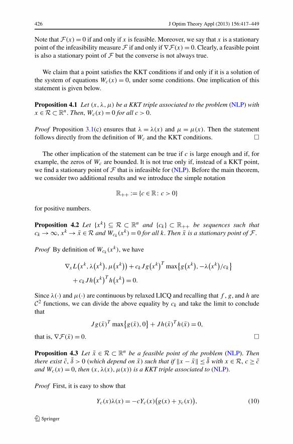
Note that F (x) = 0 if and only if x is feasible. Moreover, we say that x is a stationarypoint of the infeasibility measure F if and only if ∇F (x) = 0. Clearly, a feasible pointis also a stationary point of F but the converse is not always true.
We claim that a point satisfies the KKT conditions if and only if it is a solution ofthe system of equations Wc(x) = 0, under some conditions. One implication of thisstatement is given below.
Proposition 4.1 Let (x,λ,μ) be a KKT triple associated to the problem (NLP) withx ∈ R ⊂ R
n. Then, Wc(x) = 0 for all c > 0.
Proof Proposition 3.1(c) ensures that λ = λ(x) and μ = μ(x). Then the statementfollows directly from the definition of Wc and the KKT conditions. �
The other implication of the statement can be true if c is large enough and if, forexample, the zeros of Wc are bounded. It is not true only if, instead of a KKT point,we find a stationary point of F that is infeasible for (NLP). Before the main theorem,we consider two additional results and we introduce the simple notation
R++ := {c ∈ R : c > 0}for positive numbers.
Proposition 4.2 Let {xk} ⊆ R ⊂ Rn and {ck} ⊂ R++ be sequences such that
ck → ∞, xk → x ∈ R and Wck(xk) = 0 for all k. Then x is a stationary point of F .
Proof By definition of Wck(xk), we have
∇xL(xk,λ
(xk
),μ
(xk
)) + ckJg(xk
)T max{g(xk
),−λ
(xk
)/ck
}
+ ckJh(xk
)Th(xk
) = 0.
Since λ(·) and μ(·) are continuous by relaxed LICQ and recalling that f , g, and h areC 2 functions, we can divide the above equality by ck and take the limit to concludethat
Jg(x)T max{g(x),0
} + Jh(x)T h(x) = 0,
that is, ∇F (x) = 0. �
Proposition 4.3 Let x ∈ R ⊂ Rn be a feasible point of the problem (NLP). Then
there exist c, δ > 0 (which depend on x) such that if ‖x − x‖ ≤ δ with x ∈ R, c ≥ c
and Wc(x) = 0, then (x,λ(x),μ(x)) is a KKT triple associated to (NLP).
Proof First, it is easy to show that
Yc(x)λ(x) = −cYc(x)(g(x) + yc(x)
), (10)
J Optim Theory Appl (2013) 156:417–449 427
where Yc(x) := diag((yc)1(x), . . . , (yc)m(x)) is a diagonal matrix with diagonal en-tries (yc)i(x), i = 1, . . . ,m. Hence, from (4), we obtain
Jg(x)∇xL(x,λ(x),μ(x)
) = −ζ 2G(x)2λ(x)
= −ζ 2G(x)(G(x) + Yc(x)
)λ(x) + ζ 2G(x)Yc(x)λ(x)
= −ζ 2G(x)Λ(x)(g(x) + yc(x)
) + ζ 2G(x)Yc(x)λ(x).
Combining the last result with (10), we have
1
cJg(x)∇xL
(x,λ(x),μ(x)
) = −ζ 2G(x)
(1
cΛ(x) + Yc(x)
)(g(x) + yc(x)
).
And the definition of Wc gives
1
cJg(x)Wc(x) = 1
cJg(x)∇xL
(x,λ(x),μ(x)
) + Jg(x)Jg(x)T(g(x) + yc(x)
)
+ Jg(x)Jh(x)T h(x)
= −ζ 2G(x)
(1
cΛ(x) + Yc(x)
)(g(x) + yc(x)
)
+ Jg(x)Jg(x)T(g(x) + yc(x)
) + Jg(x)Jh(x)T h(x). (11)
Moreover, Eq. (5) yields
Jh(x)∇xL(x,λ(x),μ(x)
) = −ζ 2H(x)2μ(x),
and thus
1
cJh(x)Wc(x) = −1
cζ 2H(x)2μ(x) + Jh(x)Jg(x)T
(g(x) + yc(x)
)
+ Jh(x)Jh(x)T h(x)
= Jh(x)Jg(x)T(g(x) + yc(x)
)
+(
Jh(x)Jh(x)T − 1
cζ 2H(x)M(x)
)h(x). (12)
Combining the results from (11) and (12), we can write
1
c
[Jg(x)
Jh(x)
]Wc(x) = Kc(x)
[g(x) + yc(x)
h(x)
], (13)
with
Kc(x) :=[
(Kc(x))1 Jg(x)Jh(x)T
Jh(x)Jg(x)T (Kc(x))2
],
where(Kc(x)
)1 := Jg(x)Jg(x)T − ζ 2G(x)
((1/c)Λ(x) + Yc(x)
),
428 J Optim Theory Appl (2013) 156:417–449
(Kc(x)
)2 := Jh(x)Jh(x)T − (1/c)ζ 2H(x)M(x).
Observing that x is feasible, if c → ∞, then we have yc(x) → −g(x) and, therefore,Kc(x) → N(x). Since relaxed LICQ implies that N(x) is nonsingular, by continuity,there exist c and δ such that if ‖x − x‖ ≤ δ, c ≥ c, then Kc(x) is also nonsingular.
Now, consider any x and c such that ‖x − x‖ ≤ δ, c ≥ c and Wc(x) = 0. ThenEq. (13) implies that g(x) + yc(x) = 0 and h(x) = 0 because Kc(x) is nonsingular.Plugging these equations into the definition of Wc gives ∇xL(x,λ(x),μ(x)) = 0.Furthermore,
g(x) + yc(x) = 0 ⇔ max{g(x),−λ(x)/c
} = 0 ⇒ 0 ≥ g(x) ⊥ λ(x) ≥ 0,
and we conclude that (x,λ(x),μ(x)) is a KKT triple. �
Combining these results, we now obtain the following theorem.
Theorem 4.1 Let {xk} ⊆ R ⊂ Rn and {ck} ⊂ R++ be sequences such that ck → ∞
and Wck(xk) = 0 for all k. Also, consider {xkj } a subsequence of {xk} such that
xkj → x ⊂ R. Then, either there exists K such that (xkj , λ(xkj ),μ(xkj )) is a KKTtriple associated to (NLP) for all kj > K , or x is a stationary point of F that isinfeasible for (NLP).
Proof By Proposition 4.2, the point x is stationary of F . If x is feasible, then we canconclude, using the Proposition 4.3, that there exists K such that (xkj , λ(xkj ),μ(xkj ))
is KKT for all kj > K . �
Observe that a subsequence {xkj } of the above theorem exists if, for example, {xk}is bounded. The next result is an immediate consequence of this theorem. But in thiscase, we assume that all stationary points of the infeasibility measure F are feasible.This property holds if, for example, the functions gi , i = 1, . . . ,m are convex and hi ,i = 1, . . . , p are affine, which was assumed in André and Silva’s work [1]. The prop-erty also holds under the extended Mangasarian–Fromovitz constraint qualification,used by Di Pillo and Grippo [3].
Corollary 4.1 Assume that there exists c > 0 such that the set
Z := {x ∈ R
n : Wc(x) = 0, c > c}
is bounded with Z ⊂ R. Assume that all stationary points of F are feasible for (NLP).Then, there exists c > 0 such that if Wc(x) = 0 and c > c then (x,λ(x),μ(x)) is aKKT triple associated to (NLP).
Proof Suppose that there is no such c. So, there exist sequences {xk} ⊂ Rn and {ck} ⊂
R++ with Wck(xk) = 0 and ck → ∞ and such that (xk, λ(xk),μ(xk)) is not KKT.
But for ck > c, we have xk ∈ Z, which is bounded. So, there exists a convergentsubsequence {xkj } of {xk}. This is not possible from Theorem 4.1 and because thereis no stationary point of F that is infeasible. �
J Optim Theory Appl (2013) 156:417–449 429
A drawback of the above result is the boundedness assumption, which is not easilyverifiable. For nonlinear complementarity problems, that is, a particular case of vari-ational inequalities, the boundedness was ensured by exploiting coercivity or mono-tonicity properties of the problem data [1]. For nonlinear programming, one approachis to use an extraneous compact set containing the problem solutions as in [2, 3, 11].In this case, the sequence generated by an unconstrained algorithm could cross theboundary of this set, where the exactness property does not hold, or could not admit alimit point. To overcome such difficulty, the incorporation of barrier terms in the ex-act penalty function has been investigated [15, 18]. As a future work, we could extendthe results given here to construct these functions, called exact barrier functions [18].
Let us show now that KKT points are not only equivalent, under some assump-tions, to the system of equations Wc(x) = 0, but also to the system ∇wc(x) = 0,where wc is defined in (7).
Corollary 4.2 Let x ∈ R ⊂ Rn be a feasible point of (NLP). Then, there exist
c, δ > 0 (which depend on x) such that if ‖x − x‖ ≤ δ with x ∈ R, c ≥ c and∇wc(x) = 0, then (x,λ(x),μ(x)) is a KKT triple associated to (NLP).
Proof The proof is analogous to the proof of Proposition 4.3. In this case, we have
Kc(x) :=[(Kc(x))11 (Kc(x))12(Kc(x))21 (Kc(x))22
],
where
(Kc(x)
)11 := Jg(x)Jg(x)T − ζ 2G(x)
(1
cΛ(x) + Yc(x)
)+ 1
cJg(x)Jλ(x)T ,
(Kc(x)
)12 := Jg(x)Jh(x)T + 1
cJg(x)Jμ(x)T ,
(Kc(x)
)21 := Jh(x)Jg(x)T + 1
cJh(x)Jλ(x)T ,
(Kc(x)
)22 := Jh(x)Jh(x)T − 1
cζ 2H(x)M(x) + 1
cJh(x)Jμ(x)T .
Taking c → ∞, we can also conclude that Kc(x) → N(x) and the result follows. �
Corollary 4.3 Let {xk} ⊆ R ⊂ Rn and {ck} ⊂ R++ be sequences such that ck → ∞
and ∇wck(xk) = 0 for all k. Consider {xkj } a subsequence of {xk} with xkj → x ⊂ R.
Then, either there exists K such that (xkj , λ(xkj ),μ(xkj )) is a KKT triple associatedto (NLP) for all kj > K , or x is a stationary point of F that is infeasible for (NLP).
Proof It is easy to show that Proposition 4.2 still holds if we replace Wc with ∇wc.Then, the results follows directly from the proof of Theorem 4.1, replacing the Propo-sition 4.3 with Corollary 4.2. �
We proceed now to the equivalence of minimizers of (NLP) and the unconstrainedpenalized problem. Denote by Gf and Lf the sets of global and local solutions
430 J Optim Theory Appl (2013) 156:417–449
of (NLP), respectively. Moreover, for each c > 0, denote the sets of global and localsolutions of the penalized problem minx wc(x), respectively, by Gw(c) and Lw(c).First, let us prove that wc is a weakly exact penalty function for the problem (NLP)in the sense of [3, 18], where we remove the extraneous compact set.
Definition 4.2 The function wc is a weakly exact penalty function for (NLP) if andonly if there exists some c > 0 such that Gw(c) = Gf for all c ≥ c.
The following assumption is required to the proof.
Assumption 4.1 It holds that ∅ = Gf ⊂ R and Lw(c) ⊂ R for c large enough. Notethat the last one implies Gw(c) ⊂ R for c sufficiently large.
Before presenting the main theorem concerning global minimizers, let us considersome additional results.
Lemma 4.1 The function wc defined in (7) at x ∈ Rn can be written as
wc(x) = f (x) + ⟨λ(x), g(x) + yc(x)
⟩ + c
2
∥∥g(x) + yc(x)∥∥2
+ ⟨μ(x),h(x)
⟩ + c
2
∥∥h(x)∥∥2
.
Proof Observe that
⟨λ(x), g(x) + yc(x)
⟩ + c
2
∥∥g(x) + yc(x)∥∥2
= ⟨λ(x), g(x)
⟩ + c
2
∥∥g(x)∥∥2 + ⟨
λ(x), yc(x)⟩ + c
2
∥∥yc(x)∥∥2 + c
⟨g(x), yc(x)
⟩
= ⟨λ(x), g(x)
⟩ + c
2
∥∥g(x)∥∥2 +
⟨yc(x),
c
2yc(x) − c
(−λ(x)
c− g(x)
)⟩. (14)
Let us consider two cases:
1. For i such that [yc(x)]i = −λi(x)/c − gi(x), we have
[yc(x)
]i
(c
2
[yc(x)
]i− c
(−λi(x)
c− gi(x)
))= − c
2
[yc(x)
]2i.
2. Otherwise, for i such that [yc(x)]i = 0, we have
[yc(x)
]i
(c
2
[yc(x)
]i− c
(−λi(x)
c− gi(x)
))= 0 = − c
2
[yc(x)
]2i.
Thus, (14) is equivalent to
⟨λ(x), g(x)
⟩ + c
2
∥∥g(x)∥∥2 − c
2
∥∥yc(x)∥∥2
,
and the conclusion follows. �
J Optim Theory Appl (2013) 156:417–449 431
Lemma 4.2 Let (x,λ,μ) be a KKT triple associated to the problem (NLP) such thatx ∈ R. Then, wc(x) = f (x) for all c > 0.
Proof Since x satisfies relaxed LICQ, λ(x) = λ. From the KKT conditions, h(x) = 0and 0 ≤ λ(x) ⊥ g(x) ≤ 0, which is equivalent to g(x) + yc(x) = 0. Then the prooffollows from the formula of wc given in Lemma 4.1. �
Proposition 4.4 Let {xk} ⊆ R ⊂ Rn and {ck} ⊂ R++ be sequences such that {xk}
is bounded, ck → ∞ and xk ∈ Gw(ck) for all k. If Assumption 4.1 holds, then thereexists K such that xk ∈ Gf for all k > K .
Proof Assume that the assertion is false, that is, for all K , there exists k > K such thatxk /∈ Gf . First, let x ∈ Gf , which exists by Assumption 4.1. Since x is a KKT pointand satisfies relaxed LICQ (also from Assumption 4.1), we have, from Lemma 4.2,
wck
(xk
) ≤ wck(x) = f (x) (15)
for all k. The boundedness assumption of {xk} guarantees that there exists a sub-sequence of {xk} converging to x ∈ R
n. Without loss of generality, we can writelimk→∞ xk = x. So, taking the supremum limit in both sides of (15) gives
lim supk→∞
wck
(xk
) ≤ f (x). (16)
Now, from Lemma 4.1, wckcan be written as
wck
(xk
) = f(xk
) + ⟨λ(xk
), g
(xk
) + yck
(xk
)⟩ + ck
2
∥∥g(xk
) + yck
(xk
)∥∥2
+ ⟨μ
(xk
), h
(xk
)⟩ + ck
2
∥∥h(xk
)∥∥2.
Thus, inequality (16) implies, by continuity of the involved functions, that h(x) = 0and g(x) + max{0,−g(x)} = 0, which implies g(x) ≤ 0. Moreover, it is easy to seethat f (x) ≤ lim supk→∞ wck
(xk). Therefore, f (x) ≤ f (x) and x ∈ X, that is, x ∈ Gf .Since x is feasible and satisfies relaxed LICQ by Assumption 4.1, there exist c and
δ as in the Corollary 4.2. Let K be sufficiently large such that ‖xk − x‖ ≤ δ, ck ≥ c
and xk ∈ Gw(ck) ⊂ R for all k > K . Since xk ∈ Gw(ck) implies ∇wck(xk) = 0, the
same corollary ensures that xk is KKT, and thus feasible, for all k > K . Moreover,Lemma 4.2 and inequality (15) yield
f(xk
) = wck
(xk
) ≤ f (x)
for all k > K . We conclude that for such K , xk ∈ Gf for all k > K , which gives acontradiction. �
Proposition 4.5 Suppose that Assumption 4.1 holds. Then Gw(c) ⊆ Gf implies thatGw(c) = Gf for all c > 0.
432 J Optim Theory Appl (2013) 156:417–449
Proof Let c > 0 and x ∈ Gw(c). As Gw(c) ⊆ Gf , x is a KKT point, and thus, byLemma 4.2, wc(x) = f (x). On the other hand, let x ∈ Gf such that x = x. Since x
is also a KKT point and satisfies relaxed LICQ by Assumption 4.1, once again byLemma 4.2, we have wc(x) = f (x). Therefore, by the definition of global solutions,
wc(x) = f (x) = f (x) = wc(x).
We conclude that x ∈ Gw(c) and the result follows. �
The above two propositions can be put together and the result is as follows.
Theorem 4.2 If there exists c > 0 such that Z := ⋃c≥c Gw(c) is bounded and As-
sumption 4.1 holds, then wc is a weakly exact penalty function for the problem.
Proof From Proposition 4.5, it is sufficient to show that there exist c > 0 such thatGw(c) ⊆ Gf for all c ≥ c. Suppose that there are sequences {xk} ⊂ Z and {ck} ⊂ R++with ck ≥ c, ck → ∞ and xk ∈ Gw(ck) for all k. Since Z is bounded, Proposition 4.4guarantees that there exists K such that xk ∈ Gf for all k > K . The result followstaking c = cK . �
The drawback of the definition of weakly exact penalty functions is that uncon-strained minimization algorithms do not ensure to find global solutions in general.With this in mind, we prove that wc is essentially an exact penalty function. Onceagain, following [3, 18] and removing the extraneous compact set, we have the fol-lowing definition.
Definition 4.3 The function wc is an exact penalty function for (NLP) if and only ifthere exists c > 0 such that Gw(c) = Gf and Lw(c) ⊆ Lf for all c ≥ c.
In other words, wc is an exact penalty if it is weakly exact and any local minimizerof the unconstrained problem is a local solution of the constrained one, when c issufficiently large.
First, let us show that the equality from Lemma 4.2 becomes an inequality if theconsidered point is not KKT but only feasible.
Lemma 4.3 Let x ∈ Rn be a feasible point for (NLP). Then, wc(x) ≤ f (x) for all
c > 0.
Proof Fix some c > 0. From Lemma 4.1, wc(x) can be written as
wc(x) = f (x) +m∑
i=1
[yc(x)
]i+ ⟨
μ(x),h(x)⟩ + c
2
∥∥h(x)∥∥2
,
where[yc(x)
]i:= λi(x)
(gi(x) + [
yc(x)]i
) + c
2
(gi(x) + [
yc(x)]i
)2.
J Optim Theory Appl (2013) 156:417–449 433
Since h(x) = 0, it is enough to see that [yc(x)]i ≤ 0 for all i = 1, . . . ,m. Thus, con-sider two cases:
1. For an index i such that [yc(x)]i = −λi(x)/c − gi(x), we have
[yc(x)
]i= λi(x)
(−λi(x)
c
)+ c
2
(−λi(x)
c
)2
= −λ2i (x)
2c≤ 0.
2. For an index i such that [yc(x)]i = 0, that is, λi(x)/c + gi(x) ≥ 0, we have
[yc(x)
]i= λi(x)gi(x) + c
2g2
i (x) = c
2gi(x)
[2
(λi(x)
c+ gi(x)
)− gi(x)
].
As gi(x) ≤ 0, the term between the box brackets is nonnegative. Thus, we have[yc(x)]i ≤ 0 and the conclusion follows. �
The results concerning local minimizers are similar to Theorem 4.1 and Corol-lary 4.3 in the sense that, if a local solution of the original problem is not recovered,then we end up in a stationary point of the infeasibility measure F that is infeasiblefor (NLP).
Theorem 4.3 Let {xk} ⊆ R ⊂ Rn and {ck} ⊂ R++ be sequences such that ck → ∞
and xk ∈ Lw(ck) for all k. Let {xkj } be a subsequence of {xk} such that xkj → x ⊂ R.If Assumption 4.1 holds, then either there exists K such that xkj ∈ Lf for all kj > K ,or x is a stationary point of F that is infeasible for (NLP).
Proof Since xkj ∈ Lw(ckj) implies ∇wckj
(xkj ) = 0 for all kj , from Corollary 4.3,
there is K such that xkj is KKT for all kj > K or x is a stationary point of F thatis infeasible. Considering the first case and fixing kj > K , from Lemma 4.2, thereexists a neighborhood V (xkj ) of xkj such that
f(xkj
) = wckj
(xkj
) ≤ wckj(x) for all x ∈ V
(xkj
).
The above statement is clearly true for all x ∈ V (xkj ) ∩ X. Thus, using Lemma 4.3,we conclude that f (xkj ) ≤ wckj
(x) ≤ f (x) for all x ∈ V (xkj ) ∩ X. This means that
xkj ∈ Lf for all kj > K , which completes the proof. �
Corollary 4.4 Assume that there exists c > 0 such that⋃
c>c Lw(c) is bounded. Con-sider also that Assumption 4.1 holds and that all stationary points of F are feasiblefor (NLP). Then, there exists c > 0 such that if x ∈ Lw(c) and c > c, then x ∈ Lf .
Proof Suppose that the statement is false. So, there exist sequences {xk} ⊂ Rn and
{ck} ⊂ R++ with xk ∈ Lw(ck) and ck → ∞ and such that xk /∈ Lf . But for ck > c, wehave xk ∈ ⋃
c>c Lw(c), which is bounded. So, there exists a convergent subsequence
{xkj } of {xk}. The contradiction follows from Theorem 4.3 and because there is nostationary point of F that is infeasible. �
434 J Optim Theory Appl (2013) 156:417–449
The previous results allow us to develop an algorithm to solve the problem (NLP).In particular, Theorem 4.1 and Corollary 4.3 show that we can find a KKT point if wesolve the systems of equations Wc(x) = 0 or ∇wc(x) = 0 for a large enough c. SinceWc is semismooth and its formula does not contain second-order terms (see (9)), asemismooth Newton method can be used to solve Wc(x) = 0. It remains to show aneasy way to choose the parameter c. Also, convergence results using the semismoothNewton method should be presented, as well as a globalization idea. The next threesections will be dedicated to these topics.
5 Updating the Penalty Parameter
As we noted before, we need a way to choose the penalty parameter c. Following [1],we consider the dynamical update of parameter proposed by Glad and Polak [7]. Theidea is to create a function, which is called test function, that measures the risk ofcomputing a zero of Wc that is not KKT. First, define the following function:
ac(x) := g(x) + yc(x) = max
{g(x),−λ(x)
c
}.
Note that for all c > 0, ac(x) = 0 is equivalent to 〈g(x), λ(x)〉 = 0, g(x) ≤ 0 andλ(x) ≥ 0. Hence, we can define a test function by
tc(x) := −∥∥Wc(x)∥∥2 + 1
cγ
(∥∥ac(x)∥∥2 + ∥∥h(x)
∥∥2),
with γ > 0. It is easy to show that tc is continuous because of the continuity of theinvolved functions. Next proposition shows that tc is in fact a test function.
Proposition 5.1 The following statements are equivalent:
(a) (x,λ(x),μ(x)) is a KKT triple associated to the problem.(b) Wc(x) = 0, ac(x) = 0 and h(x) = 0.(c) Wc(x) = 0 and tc(x) ≤ 0.
Proof It follows directly from the formulas of Wc(x), ac(x), and tc(x) and the defi-nition of KKT triple. �
Let us show now that for all x ∈ R, either x is a stationary point of F that isinfeasible for (NLP), or there exists c large enough such that tc(x) ≤ 0 for all c ≥ c
and all x in a neighborhood of x. From Proposition 5.1, this second case reveals us away to update the parameter c. More precisely, for each computation of a zero of Wc,we increase the value of c if the test tc at this point is greater that zero.
Lemma 5.1 Let S ⊆ R ⊂ Rn be a compact set with no KKT points. Then, either
there exist c, ε (which depend on S) such that ‖Wc(x)‖ ≥ ε for all x ∈ S and allc ≥ c; or there exist {xk} ⊂ S, {ck} ⊂ R++ such that ck → ∞, ‖Wck
(xk)‖ → 0 and{xk} converges to a stationary point of F that is infeasible for (NLP).
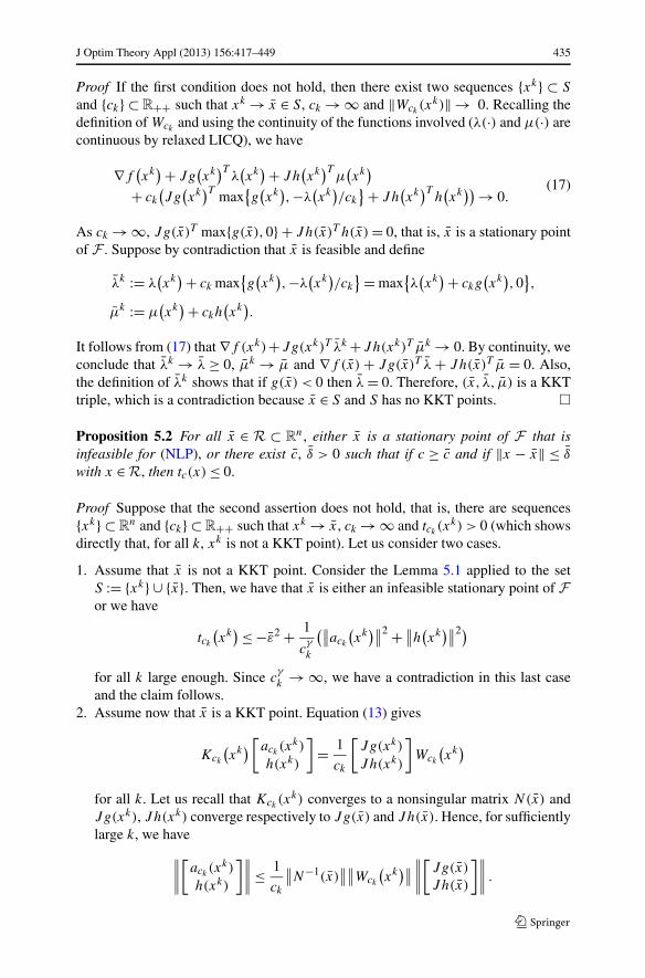
J Optim Theory Appl (2013) 156:417–449 435
Proof If the first condition does not hold, then there exist two sequences {xk} ⊂ S
and {ck} ⊂ R++ such that xk → x ∈ S, ck → ∞ and ‖Wck(xk)‖ → 0. Recalling the
definition of Wckand using the continuity of the functions involved (λ(·) and μ(·) are
continuous by relaxed LICQ), we have
∇f(xk
) + Jg(xk
)Tλ(xk
) + Jh(xk
)Tμ
(xk
)
+ ck
(Jg
(xk
)T max{g(xk
),−λ
(xk
)/ck
} + Jh(xk
)Th(xk
)) → 0.(17)
As ck → ∞, Jg(x)T max{g(x),0} + Jh(x)T h(x) = 0, that is, x is a stationary pointof F . Suppose by contradiction that x is feasible and define
λk := λ(xk
) + ck max{g(xk
),−λ
(xk
)/ck
} = max{λ(xk
) + ckg(xk
),0
},
μk := μ(xk
) + ckh(xk
).
It follows from (17) that ∇f (xk)+Jg(xk)T λk +Jh(xk)T μk → 0. By continuity, weconclude that λk → λ ≥ 0, μk → μ and ∇f (x) + Jg(x)T λ + Jh(x)T μ = 0. Also,the definition of λk shows that if g(x) < 0 then λ = 0. Therefore, (x, λ, μ) is a KKTtriple, which is a contradiction because x ∈ S and S has no KKT points. �
Proposition 5.2 For all x ∈ R ⊂ Rn, either x is a stationary point of F that is
infeasible for (NLP), or there exist c, δ > 0 such that if c ≥ c and if ‖x − x‖ ≤ δ
with x ∈ R, then tc(x) ≤ 0.
Proof Suppose that the second assertion does not hold, that is, there are sequences{xk} ⊂ R
n and {ck} ⊂ R++ such that xk → x, ck → ∞ and tck(xk) > 0 (which shows
directly that, for all k, xk is not a KKT point). Let us consider two cases.
1. Assume that x is not a KKT point. Consider the Lemma 5.1 applied to the setS := {xk} ∪ {x}. Then, we have that x is either an infeasible stationary point of For we have
tck
(xk
) ≤ −ε2 + 1
cγ
k
(∥∥ack
(xk
)∥∥2 + ∥∥h(xk
)∥∥2)
for all k large enough. Since cγ
k → ∞, we have a contradiction in this last caseand the claim follows.
2. Assume now that x is a KKT point. Equation (13) gives
Kck
(xk
)[ack
(xk)
h(xk)
]= 1
ck
[Jg(xk)
Jh(xk)
]Wck
(xk
)
for all k. Let us recall that Kck(xk) converges to a nonsingular matrix N(x) and
Jg(xk), Jh(xk) converge respectively to Jg(x) and Jh(x). Hence, for sufficientlylarge k, we have
∥∥∥∥
[ack
(xk)
h(xk)
]∥∥∥∥ ≤ 1
ck
∥∥N−1(x)∥∥∥∥Wck
(xk
)∥∥∥∥∥∥
[Jg(x)
Jh(x)
]∥∥∥∥ .
436 J Optim Theory Appl (2013) 156:417–449
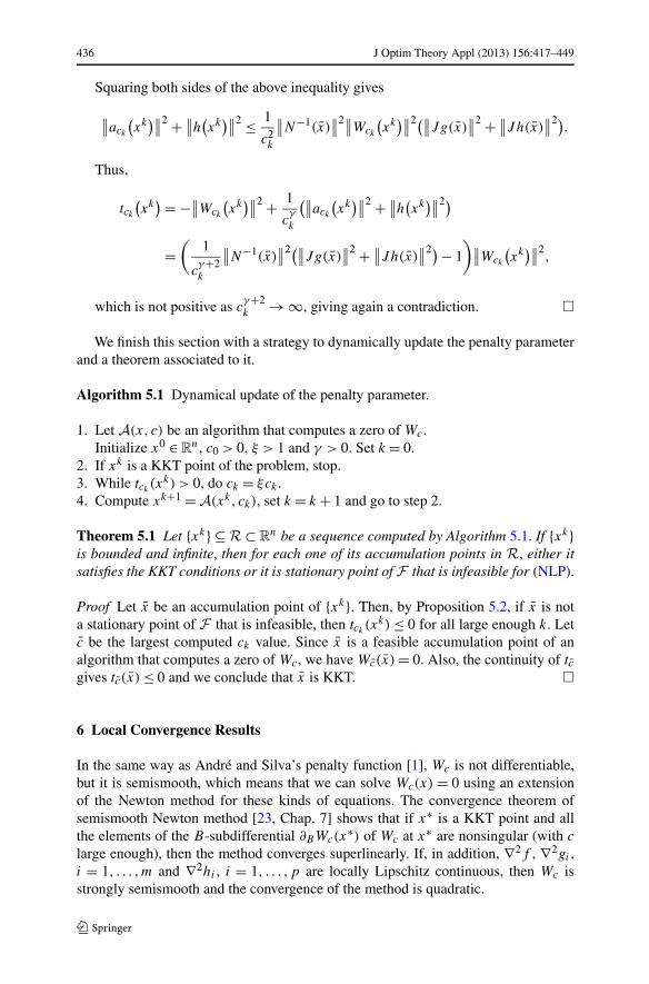
Squaring both sides of the above inequality gives
∥∥ack
(xk
)∥∥2 + ∥∥h(xk
)∥∥2 ≤ 1
c2k
∥∥N−1(x)∥∥2∥∥Wck
(xk
)∥∥2(∥∥Jg(x)∥∥2 + ∥∥Jh(x)
∥∥2).
Thus,
tck
(xk
) = −∥∥Wck
(xk
)∥∥2 + 1
cγ
k
(∥∥ack
(xk
)∥∥2 + ∥∥h(xk
)∥∥2)
=(
1
cγ+2k
∥∥N−1(x)∥∥2(∥∥Jg(x)
∥∥2 + ∥∥Jh(x)∥∥2) − 1
)∥∥Wck
(xk
)∥∥2,
which is not positive as cγ+2k → ∞, giving again a contradiction. �
We finish this section with a strategy to dynamically update the penalty parameterand a theorem associated to it.
Algorithm 5.1 Dynamical update of the penalty parameter.
1. Let A(x, c) be an algorithm that computes a zero of Wc.Initialize x0 ∈ R
n, c0 > 0, ξ > 1 and γ > 0. Set k = 0.2. If xk is a KKT point of the problem, stop.3. While tck
(xk) > 0, do ck = ξck .4. Compute xk+1 = A(xk, ck), set k = k + 1 and go to step 2.
Theorem 5.1 Let {xk} ⊆ R ⊂ Rn be a sequence computed by Algorithm 5.1. If {xk}
is bounded and infinite, then for each one of its accumulation points in R, either itsatisfies the KKT conditions or it is stationary point of F that is infeasible for (NLP).
Proof Let x be an accumulation point of {xk}. Then, by Proposition 5.2, if x is nota stationary point of F that is infeasible, then tck
(xk) ≤ 0 for all large enough k. Letc be the largest computed ck value. Since x is a feasible accumulation point of analgorithm that computes a zero of Wc, we have Wc(x) = 0. Also, the continuity of tcgives tc(x) ≤ 0 and we conclude that x is KKT. �
6 Local Convergence Results
In the same way as André and Silva’s penalty function [1], Wc is not differentiable,but it is semismooth, which means that we can solve Wc(x) = 0 using an extensionof the Newton method for these kinds of equations. The convergence theorem ofsemismooth Newton method [23, Chap. 7] shows that if x∗ is a KKT point and allthe elements of the B-subdifferential ∂BWc(x
∗) of Wc at x∗ are nonsingular (with c
large enough), then the method converges superlinearly. If, in addition, ∇2f , ∇2gi ,i = 1, . . . ,m and ∇2hi , i = 1, . . . , p are locally Lipschitz continuous, then Wc isstrongly semismooth and the convergence of the method is quadratic.
J Optim Theory Appl (2013) 156:417–449 437
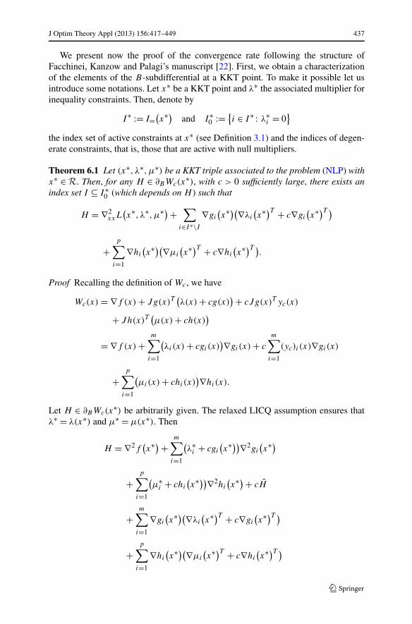
We present now the proof of the convergence rate following the structure ofFacchinei, Kanzow and Palagi’s manuscript [22]. First, we obtain a characterizationof the elements of the B-subdifferential at a KKT point. To make it possible let usintroduce some notations. Let x∗ be a KKT point and λ∗ the associated multiplier forinequality constraints. Then, denote by
I ∗ := I=(x∗) and I ∗
0 := {i ∈ I ∗ : λ∗
i = 0}
the index set of active constraints at x∗ (see Definition 3.1) and the indices of degen-erate constraints, that is, those that are active with null multipliers.
Theorem 6.1 Let (x∗, λ∗,μ∗) be a KKT triple associated to the problem (NLP) withx∗ ∈ R. Then, for any H ∈ ∂BWc(x
∗), with c > 0 sufficiently large, there exists anindex set I ⊆ I ∗
0 (which depends on H ) such that
H = ∇2xxL
(x∗, λ∗,μ∗) +
∑
i∈I∗\I∇gi
(x∗)(∇λi
(x∗)T + c∇gi
(x∗)T )
+p∑
i=1
∇hi
(x∗)(∇μi
(x∗)T + c∇hi
(x∗)T )
.
Proof Recalling the definition of Wc, we have
Wc(x) = ∇f (x) + Jg(x)T(λ(x) + cg(x)
) + cJg(x)T yc(x)
+ Jh(x)T(μ(x) + ch(x)
)
= ∇f (x) +m∑
i=1
(λi(x) + cgi(x)
)∇gi(x) + c
m∑
i=1
(yc)i(x)∇gi(x)
+p∑
i=1
(μi(x) + chi(x)
)∇hi(x).
Let H ∈ ∂BWc(x∗) be arbitrarily given. The relaxed LICQ assumption ensures that
λ∗ = λ(x∗) and μ∗ = μ(x∗). Then
H = ∇2f(x∗) +
m∑
i=1
(λ∗
i + cgi
(x∗))∇2gi
(x∗)
+p∑
i=1
(μ∗
i + chi
(x∗))∇2hi
(x∗) + cH
+m∑
i=1
∇gi
(x∗)(∇λi
(x∗)T + c∇gi
(x∗)T )
+p∑
i=1
∇hi
(x∗)(∇μi
(x∗)T + c∇hi
(x∗)T )
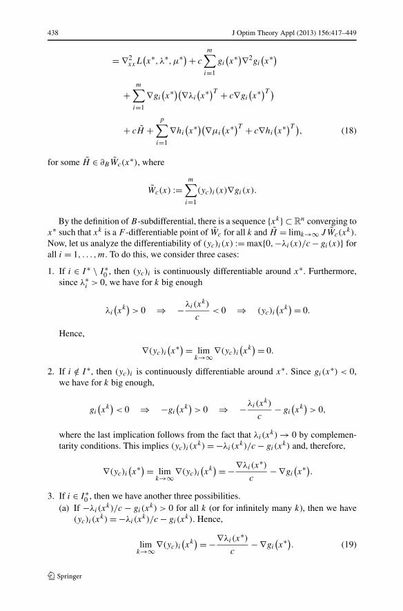
438 J Optim Theory Appl (2013) 156:417–449
= ∇2xxL
(x∗, λ∗,μ∗) + c
m∑
i=1
gi
(x∗)∇2gi
(x∗)
+m∑
i=1
∇gi
(x∗)(∇λi
(x∗)T + c∇gi
(x∗)T )
+ cH +p∑
i=1
∇hi
(x∗)(∇μi
(x∗)T + c∇hi
(x∗)T )
, (18)
for some H ∈ ∂BWc(x∗), where
Wc(x) :=m∑
i=1
(yc)i(x)∇gi(x).
By the definition of B-subdifferential, there is a sequence {xk} ⊂ Rn converging to
x∗ such that xk is a F -differentiable point of Wc for all k and H = limk→∞ JWc(xk).
Now, let us analyze the differentiability of (yc)i(x) := max{0,−λi(x)/c − gi(x)} forall i = 1, . . . ,m. To do this, we consider three cases:
1. If i ∈ I ∗ \ I ∗0 , then (yc)i is continuously differentiable around x∗. Furthermore,
since λ∗i > 0, we have for k big enough
λi
(xk
)> 0 ⇒ −λi(x
k)
c< 0 ⇒ (yc)i
(xk
) = 0.
Hence,
∇(yc)i(x∗) = lim
k→∞∇(yc)i(xk
) = 0.
2. If i /∈ I ∗, then (yc)i is continuously differentiable around x∗. Since gi(x∗) < 0,
we have for k big enough,
gi
(xk
)< 0 ⇒ −gi
(xk
)> 0 ⇒ −λi(x
k)
c− gi
(xk
)> 0,
where the last implication follows from the fact that λi(xk) → 0 by complemen-
tarity conditions. This implies (yc)i(xk) = −λi(x
k)/c − gi(xk) and, therefore,
∇(yc)i(x∗) = lim
k→∞∇(yc)i(xk
) = −∇λi(x∗)
c− ∇gi
(x∗).
3. If i ∈ I ∗0 , then we have another three possibilities.
(a) If −λi(xk)/c − gi(x
k) > 0 for all k (or for infinitely many k), then we have(yc)i(x
k) = −λi(xk)/c − gi(x
k). Hence,
limk→∞∇(yc)i
(xk
) = −∇λi(x∗)
c− ∇gi
(x∗). (19)
J Optim Theory Appl (2013) 156:417–449 439
(b) If −λi(xk)/c − gi(x
k) < 0 for all k, we have (yc)i(xk) = 0. Then we obtain
limk→∞∇(yc)i
(xk
) = 0.
(c) If −λi(xk)/c−gi(x
k) = 0 for all k, then (yc)i will be nondifferentiable unless−∇λi(x
k)/c − ∇gi(xk) = 0. Since ∇gi(x
k) is nonzero by relaxed LICQ andc is sufficiently large, we conclude that this equality does not hold.
Define now the following index set:
I := {i ∈ I ∗
0 : equality (19) holds}.
Also note that (yc)i(x∗) = −gi(x
∗). In fact, if gi(x∗) = 0, then (yc)i(x
∗) = 0, be-cause −λ∗
i /c ≤ 0. On the other hand, if gi(x∗) < 0, in view of complementarity
conditions, we have λ∗i = 0 and so (yc)i(x
∗) = −gi(x∗). In this way, we have the
following representation of H :
H =m∑
i=1
(yc)i(x∗)∇2gi
(x∗) +
∑
i /∈I∗∇gi
(x∗)
(−∇λi(x
∗)T
c− ∇gi
(x∗)T
)
+∑
i∈I
∇gi
(x∗)
(−∇λi(x
∗)T
c− ∇gi
(x∗)T
)
= −m∑
i=1
gi
(x∗)∇2gi
(x∗)
+∑
i /∈I∗\I∇gi
(x∗)
(−∇λi(x
∗)T
c− ∇gi
(x∗)T
). (20)
Finally, putting together equalities (18) and (20), we have
H = ∇2xxL
(x∗, λ∗,μ∗) + c
m∑
i=1
gi
(x∗)∇2gi
(x∗)
+m∑
i=1
∇gi
(x∗)(∇λi
(x∗)T + c∇gi
(x∗)T )
− c
m∑
i=1
gi
(x∗)∇2gi
(x∗) −
∑
i /∈I∗\I∇gi
(x∗)(∇λi
(x∗)T + c∇gi
(x∗)T )
+p∑
i=1
∇hi
(x∗)(∇μi
(x∗)T + c∇hi
(x∗)T )
440 J Optim Theory Appl (2013) 156:417–449
= ∇2xxL
(x∗, λ∗,μ∗) +
∑
i∈I∗\I∇gi
(x∗)(∇λi
(x∗)T + c∇gi
(x∗)T )
+p∑
i=1
∇hi
(x∗)(∇μi
(x∗)T + c∇hi
(x∗)T )
,
which gives the desired result. �
In order to prove their convergence rate result, Facchinei, Kanzow, and Palagi [22]used an assumption called weak regularity, which is defined below.
Definition 6.1 A KKT triple (x∗, λ∗,μ∗) is said weakly regular if and only if, for allI ⊆ I ∗
0 , the Hessian ∇2xxL(x∗, λ∗,μ∗) is not singular on the subspace
UI := {d ∈ R
n : ⟨∇gi
(x∗), d
⟩ = 0, i ∈ I ∗ \ I,⟨∇hi
(x∗), d
⟩ = 0, i = 1, . . . , p}, (21)
or, in other words, if
PUI∇2
xxL(x∗, λ∗,μ∗)d = 0 for all d ∈ UI , d = 0,
with PUIdenoting the orthogonal projection onto UI , and for all subset I ⊆ I ∗
0 .
Since they were interested in variational inequalities, we propose related condi-tions that guarantee fast convergence, which seems more natural in the optimizationcontext. The first one is the well-known second-order sufficient condition.
Definition 6.2 A KKT triple (x∗, λ∗,μ∗) satisfies the second-order sufficient condi-tion if and only if
⟨∇2xxL
(x∗, λ∗,μ∗)d, d
⟩> 0 for all d ∈ UI∗
0∩ U0, d = 0,
where, UI∗0
is defined in (21) with I = I ∗0 and
U0 := {d ∈ R
n : ⟨∇gi
(x∗), d
⟩ ≤ 0 for all i ∈ I ∗0
}. (22)
Unfortunately, this condition is not sufficient to prove the convergence rate. Anadditional assumption that ensures fast convergence is the strict complementarity,that is, I ∗
0 = ∅. But this is a strong condition, in the sense that it does not hold inmany cases. Classical results in sequential quadratic programming [24, Chap. 18],for example, use these two conditions, but more recent works in this area [25, 26] useinstead the strong second-order sufficient condition, which we recall below.
Definition 6.3 A KKT triple (x∗, λ∗,μ∗) satisfies the strong second-order sufficientcondition if and only if
⟨∇2xxL
(x∗, λ∗,μ∗)d, d
⟩> 0 for all d ∈ UI∗
0, d = 0.
J Optim Theory Appl (2013) 156:417–449 441
This condition is also required in recent works about exact merit functions [19, 20],and ensures the convergence rate. However, it can be proved that it is more restrictivethan weak regularity.
Lemma 6.1 Let (x∗, λ∗,μ∗) be a KKT triple. If it satisfies the strong second-ordersufficient condition, then it is weakly regular.
Proof Since I ⊆ I ∗0 implies UI ⊆ UI∗
0, the strong second-order sufficient condition
can be written as
⟨∇2xxL
(x∗, λ∗,μ∗)d, d
⟩> 0 for all d ∈ UI , d = 0 and all I ⊆ I ∗
0 .
Fix I ⊆ I ∗0 and d ∈ UI with d = 0. Since PUI
is symmetric and d ∈ UI ,
0 <⟨∇2
xxL(x∗, λ∗,μ∗)d, d
⟩ = ⟨PUI
∇2xxL
(x∗, λ∗,μ∗)d, d
⟩.
This shows that PUI∇2
xxL(x∗, λ∗,μ∗)d = 0, and thus the weak regularity holds. �
Remark The converse implication is not necessarily true. Indeed, we have the follow-ing counterexample: n = 2, m = 3 and p = 0, with f (x) := −x2, g1(x) := −x2
1 +x2,g2(x) := −x1 and g3(x) := x1. In this case, we obtain x∗ = (0,0)T , I ∗ = {1,2,3}and ∇xL(x∗, λ∗) = 0 implies that λ∗
1 = 1 and λ∗2 = λ∗
3. If λ∗2 = λ∗
3 = 0, we haveI ∗
0 = {2,3}. Thus, we obtain U{2} = U{3} = U∅ = {(0,0)T }, U0 = {d ∈ R2 : d1 = 0},
and UI∗0
= {d ∈ R2 : d2 = 0}. For the case I = I ∗
0 , we have
PUI∗0∇2
xxL(x∗, λ∗)d = PUI∗
0
[−2d10
]=
[−2d10
]= 0
for all d ∈ UI∗0
, d = 0. Therefore, the weak regularity is satisfied. However,
⟨∇2xxL
(x∗, λ∗)d, d
⟩ = −2d21 ≤ 0,
which shows that the strong second-order sufficient condition is not satisfied.
Recalling that we desire a natural condition in the context of optimization, and asan alternative, we propose to use the second-order sufficient condition with anothercondition associated to the nonsingularity of the Hessian ∇2
xxL(x∗, λ∗,μ∗), which issimilar to weak regularity.
Assumption 6.1 Let (x∗, λ∗,μ∗) be a KKT triple. Then the second-order sufficientcondition (see Definition 6.2) holds and
PUI∗0∇2
xxL(x∗, λ∗,μ∗)d = 0 for all d ∈ UI∗
0\ U0, d = 0,
recalling that UI∗0
is defined in (21) for I = I ∗0 and U0 is defined in (22).
442 J Optim Theory Appl (2013) 156:417–449
Theorem 6.2 Let (x∗, λ∗,μ∗) be a KKT triple associated to the problem (NLP) withx∗ ∈ R. If Assumption 6.1 holds, then all matrices of the B-subdifferential ∂BWc(x
∗)are nonsingular for all sufficiently large c > 0.
Proof Assume for the purpose of contradiction that there are sequences {ck} ⊂ R++and {Hk} ⊂ R
n×n such that ck → +∞ and Hk ∈ ∂BWck(x∗) is singular for all k.
Then there exists {dk} ⊂ Rn with ‖dk‖ = 1, such that HT
k dk = 0 for all k and, con-sequently, 〈HT
k dk, dk〉 = 0 for all k. Consider, without loss of generality, that {dk}converges to some vector d∗ ∈ R
n. From Theorem 6.1, for each k, there is a subsetIk ⊆ I ∗
0 such that
HTk dk = ∇2
xxL(x∗, λ∗μ∗)dk +
∑
i∈I∗\Ik
⟨∇gi
(x∗), dk
⟩(∇λi
(x∗) + ck∇gi
(x∗))
+p∑
i=1
⟨∇hi
(x∗), dk
⟩(∇μi
(x∗) + ck∇hi
(x∗)). (23)
Since there are finitely many subsets Ik , we may assume that Ik = I for all k. Thus,
⟨HT
k dk, dk⟩ = ⟨∇2
xxL(x∗, λ∗,μ∗)dk, dk
⟩ +∑
i∈I∗\I
⟨∇gi
(x∗), dk
⟩⟨∇λi
(x∗), dk
⟩
+ ck
∑
i∈I∗\I
⟨∇gi
(x∗), dk
⟩2 +p∑
i=1
⟨∇hi
(x∗), dk
⟩⟨∇μi
(x∗), dk
⟩
+ ck
p∑
i=1
⟨∇hi
(x∗), dk
⟩2.
Dividing the above expression by ck , taking ck → +∞ and recalling that, for all k,〈HT
k dk, dk〉 = 0, it follows that
∑
i∈I∗\I
⟨∇gi
(x∗), dk
⟩2 +p∑
i=1
⟨∇hi
(x∗), dk
⟩2 → 0,
which implies that 〈∇gi(x∗), d∗〉 = 0 for all i ∈ I ∗ \ I and 〈∇hi(x
∗), d∗〉 = 0 for alli = 1, . . . , p, that is, d∗ ∈ UI . Now, observe that for all k,
∑
i∈I∗\I
⟨∇gi
(x∗), dk
⟩∇gi
(x∗) ∈ U⊥
I andp∑
i=1
⟨∇hi
(x∗), dk
⟩∇hi
(x∗) ∈ U⊥
I .
In fact, for all d ∈ UI ,
∑
i∈I∗\I
⟨∇gi
(x∗), dk
⟩⟨∇gi
(x∗), d
⟩ = 0 andp∑
i=1
⟨∇hi
(x∗), dk
⟩⟨∇hi
(x∗), d
⟩ = 0,
J Optim Theory Appl (2013) 156:417–449 443
because of the definition of UI . This fact, the equality (23) with Ik = I , and the factthat HT
k dk = 0 for all k, show that
0 = PUI∇2
xxL(x∗, λ∗μ∗)dk + PUI
[ ∑
i∈I∗\I
⟨∇gi
(x∗), dk
⟩∇λi
(x∗)
]
+ PUI
[p∑
i=1
⟨∇hi
(x∗), dk
⟩∇μi
(x∗)
]
for all k. Taking k → ∞ in the above equality, we obtain
PUI∇2
xxL(x∗, λ∗μ∗)d∗ = 0, (24)
once again because d∗ ∈ UI .Note now that if d∗ /∈ U0, then we have a contradiction because of Assumption 6.1
and since I ⊆ I ∗0 implies UI ⊆ UI∗
0. On the other hand, if d∗ ∈ U0, then equality (24),
the fact that d∗ ∈ UI and the symmetry of PUIimply that
0 = ⟨PUI
∇2xxL
(x∗, λ∗μ∗)d∗, d∗⟩ = ⟨∇2
xxL(x∗, λ∗μ∗)d∗, d∗⟩,
which contradicts the second-order sufficient condition. �
From Lemma 6.1, it is easy to see that the convergence result above can be provedif we replace the Assumption 6.1 with the strong second-order sufficient condition orthe weak regularity.
7 Globalization and Numerical Experiments
To globalize the method, we can just use the merit function ‖Wc(·)‖2/2. But thishappens to be nondifferentiable. Besides, recalling the formulas of ∇wc and Wc in (8)and (9), we observe that a minimizer x of wc should satisfy
∇wc(x) = Wc(x) + second-order terms = 0.
Thus, a stationary point of wc is a zero of Wc, if we ignore the second-order terms.In Theorem 4.1 and Corollary 4.3, we saw that these terms are ignored when x is aKKT point because, in this case, ∇wc(x) = Wc(x) = 0. This means that we can usethe exact penalty wc as the merit function. Also, the method can be considered as aGauss–Newton-type method, in the sense that we can ignore second-order terms atthe points that we are interested in.
The final algorithm is given below.
Algorithm 7.1 Gauss–Newton-type method to minimize wc , using Wc to computethe search direction and with dynamical update of the penalty parameter.
1. Choose x0 ∈ Rn, c0 > 0, ξ > 1, ε1 ≥ 0, ε2, ε3 ∈ (0,1) and σ ∈ (0,1/2). Set k = 0.
444 J Optim Theory Appl (2013) 156:417–449
2. If ‖∇wck(xk)‖ ≤ ε1, stop.
3. While tck(xk) > 0, do ck = ξck .
4. Compute Wck(xk) and take Hk ∈ ∂BWck
(xk).5. Find dk such that Hkd
k = −Wck(xk).
6. If 〈∇wck(xk), dk〉 > −ε2‖dk‖‖∇wck
(xk)‖ or ‖dk‖ < ε3‖∇wck(xk)‖,
set dk = −∇wck(xk).
7. Find tk ∈ (0,1] such that wck(xk + tkd
k) ≤ wck(xk) + σ tk〈∇wck
(xk), dk〉 with abacktracking strategy.
8. Set xk+1 = xk + tkdk , k = k + 1 and go to step 2.
Observe that in step 6 we verify if dk is a sufficient descent direction and if thenorm condition is satisfied. If not, we replace it with the steepest descent direction.Concerning the stepsize tk , we do an Armijo-type line search at step 7. It is importantto see that for each Armijo-type iteration, we have to compute the functional valuewck
(xk + tkdk) that requires the multipliers estimates λ(xk + tkd
k) and μ(xk + tkdk),
which means to solve a linear least squares problem. Since the matrix associated tothis system of equations changes for each point, this strategy may be computationallyexpensive if many Armijo iterations are required.
To increase the robustness of the implementation, we also use nonmonotone linesearch [27] and quadratic interpolation for the backtracking strategy. When the steep-est descent direction is taken instead of the Newton direction, we use the spectralstep [28] to compute the initial stepsize of the iteration. One fundamental aspect ina globalization scheme is to verify if, eventually, the Newton direction is chosen andthe unit stepsize is taken. When one of these conditions fails, then the globalizationprocedure deteriorates the superlinear convergence and the so-called “Maratos effect”occurs. Unfortunately, we have no formal proof that ensures that the “Maratos effect”does not show up. However, this seems not to affect the numerical behavior, as wewill discuss later.
Let us now begin to describe the implementation of the Algorithm 7.1. We im-plemented it in Python and we consider the following values of parameters: γ = 2,ξ = 10, ζ = 2.0, σ = 10−4 (following [1]) and ε1 = ε2 = ε3 = 10−8 (following [29,30]). To compute an element of the B-subdifferential ∂BWck
(xk), we also have tochoose a convexity parameter because of the maximum function contained in the for-mula of Wck
(xk). We choose the one that vanishes λi and not gi . Besides, we use theroutine lstsq from SciPy library to solve the linear least squares problem associ-ated to the estimates. Moreover, if Hk ∈ ∂BWck
(xk) is computationally singular, thenwe add on it a multiple of the identity matrix in order to solve the system of equations(step 5 of Algorithm 7.1). At step 2, we also consider as an alternative stopping cri-terion that the point satisfies the KKT conditions within a prefixed tolerance of 10−8.Furthermore, we limit the maximum number of iterations in 100000 and the time in10 minutes. With all these implementation details, numerical experiments was doneusing the CUTE collection [31] modeled in AMPL [32].
We considered all constrained problems of such collection with at most 300 vari-ables and constraints, which returns 328 problems. In order to have a comparisonparameter, we also tested these problems with ALGENCAN [29, 30], an augmentedLagrangian method. The method proposed here does not make distinctions betweenbox constraints and the other inequality ones as ALGENCAN do. Thus, to make
J Optim Theory Appl (2013) 156:417–449 445
a more significant comparison, we modify ALGENCAN’s interface with AMPL inorder to not differentiate these box constraints. We also cut off extrapolations, New-tonian steps and acceleration of this solver, in order to make ALGENCAN to behaveas a pure augmented Lagrangian algorithm. Moreover, in the same way of ALGEN-CAN, we make the initial penalty parameter of the exact penalty method being de-pendent of the problem. Since updates of the penalty parameter with the test functionare not so frequent [1, 7], we also add a dynamical update of parameter using ananalysis of the infeasibility measure used by ALGENCAN.
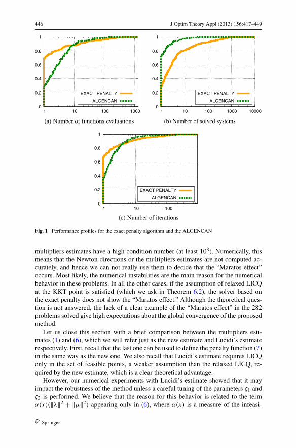
First, let us point out that the computational time is not considered here, becausethe implementation of the exact penalty method is not mature as ALGENCAN. Weverified that ALGENCAN solved 297 problems, while the exact penalty methodsolved 282. If we ignore the (few) cases where the implementations fail becauseof functions evaluations, we have an effective robustness of 92.52 % and 87.31 %,respectively for ALGENCAN and for the exact penalty. Most of the failures of theexact penalty are due to the high condition numbers of the matrices associated to sys-tem of equations for the computation of the multipliers estimate, or the big values ofpenalty parameters, which cause numerical instabilities. Furthermore, in 7 problems,the exact penalty returned a stationary point of the infeasibility measure F that is in-feasible. Concerning the total number of functions evaluations for each problem, theexact penalty method performs better. To clarify this fact, a performance profile [33],drawn on the subset of problems solved by both solvers, is presented in Fig. 1a. Thisresult is interesting particularly for problems such that these evaluations are compu-tationally expensive, which clearly appears in the literature [34, 35].
On the other hand, the total number of systems of equations is smaller withALGENCAN, as shown in Fig. 1b. We note, however, that this comparison is nottotally appropriate because it makes sense only in the case that the number of vari-ables n do not differ a lot from the total number of constraints m + p. Let us recallthat Algorithm 7.1 solves basically one n × n system for iteration during the com-putation of Newton’s step, and at least one (n + m + p) × (m + p) system duringthe Armijo-type line search. In ALGENCAN’s case, we only have n × n systemsto solve for each inner iteration. Despite this, the comparison clearly shows that theArmijo-type line search is expensive, and thus should be avoided.
Another result refers to the number of iterations of the exact penalty against thenumber of inner iterations of ALGENCAN. In such a case, the exact penalty has theadvantage, as it could be seen in Fig. 1c. Observe that the number of iterations in theexact penalty method is equal to the number of n × n systems, except for rare caseswhen the B-subdifferential matrix is computationally singular. This result suggeststhat if we replace the Armijo-type line search for some strategy that requires few(n + m + p) × (m + p) systems, then the total number of systems of equations inboth algorithms could not differ so much. For further research, trust region methodscould be a replacement for the Armijo-type line search.
As we noted before, we could not ensure that the “Maratos effect” does not oc-cur, so we also search for a counterexample in the CUTE problem set that we hadconsidered. We observe that there are 10 instances where the Newton directions withunit stepsizes are not eventually taken. However, in these cases the matrices asso-ciated to the systems of equations for the computation of Newton directions or the
446 J Optim Theory Appl (2013) 156:417–449
Fig. 1 Performance profiles for the exact penalty algorithm and the ALGENCAN
multipliers estimates have a high condition number (at least 108). Numerically, thismeans that the Newton directions or the multipliers estimates are not computed ac-curately, and hence we can not really use them to decide that the “Maratos effect”occurs. Most likely, the numerical instabilities are the main reason for the numericalbehavior in these problems. In all the other cases, if the assumption of relaxed LICQat the KKT point is satisfied (which we ask in Theorem 6.2), the solver based onthe exact penalty does not show the “Maratos effect.” Although the theoretical ques-tion is not answered, the lack of a clear example of the “Maratos effect” in the 282problems solved give high expectations about the global convergence of the proposedmethod.
Let us close this section with a brief comparison between the multipliers esti-mates (1) and (6), which we will refer just as the new estimate and Lucidi’s estimaterespectively. First, recall that the last one can be used to define the penalty function (7)in the same way as the new one. We also recall that Lucidi’s estimate requires LICQonly in the set of feasible points, a weaker assumption than the relaxed LICQ, re-quired by the new estimate, which is a clear theoretical advantage.
However, our numerical experiments with Lucidi’s estimate showed that it mayimpact the robustness of the method unless a careful tuning of the parameters ζ1 andζ2 is performed. We believe that the reason for this behavior is related to the termα(x)(‖λ‖2 + ‖μ‖2) appearing only in (6), where α(x) is a measure of the infeasi-
J Optim Theory Appl (2013) 156:417–449 447
bility of x. This term introduces a tendency to select small multipliers whenever x
is infeasible. In particular, infeasibility with respect to a single constraint impactsthe multipliers associated to the other constraints. This behavior may lead to a largerincrease of the penalty parameter, to achieve feasibility, when compared to an exactpenalty based on the new estimate.
Depending on the values of the parameters ζ1 and ζ2, the necessity of a larger c
can also be observed using the 328 problems from the CUTE test set. A large c canincrease the possibility of converging to a stationary point of the infeasibility mea-sure F that is infeasible for (NLP). In fact, while working on a Lucidi’s version of thecode we could see that it would fail returning such points in 7 up to 15 test problems,depending on the choice of parameters. This contrasts with a shorter range from 7 upto 10 problems observed with the penalty using the new multipliers estimate. Note,however, that with a careful choice of the parameters, both penalties solved 282 prob-lems. The number of failures due to convergence to stationary points of F is also thesame (in the case, 7 problems). Such result was established using the parametersζ1 = ζ2 = 2 and it was the best robustness result that we obtained using Lucidi’s es-timate. One might conjecture that using small values for ζ2 yields better robustness,but we could not confirm this behavior in our framework. Actually, for ζ2 = 10−6 thenumber of problems solved decreases slightly to 279. Using ζ2 = 10−8 the numberof problems solved decreases more significantly to 266.
Finally, a natural question is if the multipliers estimate proposed by Glad andPolak in [7] performs well or not in practice. We recall that such estimate is obtainedby solving a problem like (1) without the term ‖H(x)μ‖2. We end up solving 271problems from the CUTE test set that we are considering, and all unsolved problemsby the new estimate were also not solved when using Glad and Polak’s estimate.
8 Conclusion
As far as we know, numerical experiments with medium-sized test problems andexact merit functions for optimization (like Di Pillo and Grippo’s [3]) had not beenconsidered yet in the literature, except for exact augmented Lagrangians in the recentpaper of Di Pillo et al. [20]. Here, we extend the penalty function for variationalinequalities [1] in order to solve optimization problems, and we observe that in thiscase Di Pillo and Grippo’s exact penalty could be used as a merit function. Furtherinvestigations into the implementation should be done, in particular, concerning theexpensive Armijo-type line search.
Acknowledgements This work was supported by PRONEX-Optimization (PRONEX-CNPq/FAPERJE-26/171.510/2006-APQ1), FAPESP (Grants 2010/20572-0, 2007/53471-0, 2006/53768-0, and 2005/02163-8) and CNPq (Grants 303030/2007-0 and 474138/2008-9). We are also grateful to the refereesfor their helpful comments.
References
1. André, T.A., Silva, P.J.S.: Exact penalties for variational inequalities with applications to nonlinearcomplementarity problems. Comput. Optim. Appl. 47(3), 401–429 (2010)
448 J Optim Theory Appl (2013) 156:417–449
2. Di Pillo, G., Grippo, L.: An exact penalty method with global convergence properties. Math. Program.36, 1–18 (1986)
3. Di Pillo, G., Grippo, L.: Exact penalty functions in constrained optimization. SIAM J. Control Optim.27(6), 1333–1360 (1989)
4. Zangwill, W.I.: Nonlinear programming via penalty functions. Manag. Sci. 13, 344–358 (1967)5. Bertsekas, D.P.: Nonlinear Programming, 2nd edn. Athena Scientific, Belmont (1999)6. Fletcher, R.: A class of methods for nonlinear programming with termination and convergence prop-
erties. In: Abadie, J. (ed.) Integer and Nonlinear Programming, pp. 157–173. North-Holland, Amster-dam (1970)
7. Glad, T., Polak, E.: A multiplier method with automatic limitation of penalty growth. Math. Program.17(2), 140–155 (1979)
8. Mukai, H., Polak, E.: A quadratically convergent primal-dual algorithm with global convergence prop-erties for solving optimization problems with equality constraints. Math. Program. 9(3), 336–349(1975)
9. Di Pillo, G., Grippo, L.: A new class of augmented Lagrangians in nonlinear programming. SIAM J.Control Optim. 17(5), 618–628 (1979)
10. Di Pillo, G., Grippo, L.: A new augmented Lagrangian function for inequality constraints in nonlinearprogramming. J. Optim. Theory Appl. 36(4), 495–519 (1982)
11. Di Pillo, G., Grippo, L.: A continuously differentiable exact penalty function for nonlinear program-ming problems with inequality constraints. SIAM J. Control Optim. 23(1), 72–84 (1985)
12. Hestenes, M.R.: Multiplier and gradient methods. J. Optim. Theory Appl. 4, 303–320 (1969)13. Powell, M.J.D.: A method for nonlinear constraints in minimization problems. In: Fletcher, R. (ed.)
Optimization, pp. 283–298. Academic Press, New York (1969)14. Rockafellar, R.T.: Augmented Lagrange multiplier functions and duality in nonconvex programming.
SIAM J. Control Optim. 12(2), 268–285 (1974)15. Lucidi, S.: New results on a continuously differentiable exact penalty function. SIAM J. Optim. 2(4),
558–574 (1992)16. Auslender, A., Teboulle, M.: Lagrangian duality and related multiplier methods for variational in-
equality problems. SIAM J. Optim. 10(4), 1097–1115 (2000)17. Bertsekas, D.P.: Constrained Optimization and Lagrange Multipliers Methods. Academic Press, New
York (1982)18. Di Pillo, G.: Exact penalty methods. In: Algorithms for Continuous Optimization: The State of the Art.
NATO ASI Series, Mathematical and Physical Sciences, vol. 434, pp. 209–254. Kluwer Academic,Dordrecht (1993)
19. Di Pillo, G., Lucidi, S.: An augmented Lagrangian function with improved exactness properties.SIAM J. Optim. 12(2), 376–406 (2001)
20. Di Pillo, G., Liuzzi, G., Lucidi, S., Palagi, L.: A truncated Newton method in an augmented La-grangian framework for nonlinear programming. Comput. Optim. Appl. 45(2), 311–352 (2010)
21. Qi, L., Sun, J.: A nonsmooth version of Newton’s method. Math. Program. 58(1–3), 353–367 (1993)22. Facchinei, F., Kanzow, C., Palagi, L.: Personal communication (2007)23. Facchinei, F., Pang, J.S.: Finite-Dimensional Variational Inequalities and Complementarity Problems,
vol. II. Springer Series in Operations Research. Springer, New York (2003)24. Nocedal, J., Wright, S.J.: Numerical Optimization, 1st edn. Springer, New York (1999)25. Jian, J.B., Tang, C.M., Hu, Q.J., Zheng, H.Y.: A feasible descent SQP algorithm for general con-
strained optimization without strict complementarity. J. Comput. Appl. Math. 180, 391–412 (2005)26. Wright, S.J.: Modifying SQP for degenerate problems. SIAM J. Optim. 13(2), 470–497 (2002)27. Grippo, L., Lampariello, F., Lucidi, S.: A nonmonotone line search technique for Newton’s method.
SIAM J. Numer. Anal. 23(4), 707–716 (1986)28. Birgin, E.G., Martínez, J.M., Raydan, M.: Nonmonotone spectral projected gradient methods for con-
vex sets. SIAM J. Optim. 10(4), 1196–1211 (2000)29. Andreani, R., Birgin, E.G., Martínez, J.M., Schuverdt, M.: On augmented Lagrangian methods with
general lower-level constraints. SIAM J. Optim. 18(4), 1286–1309 (2007)30. Andreani, R., Birgin, E.G., Martínez, J.M., Schuverdt, M.: Augmented Lagrangian methods under the
constant positive linear dependence constraint qualification. Math. Program. 111(1–2), 5–32 (2008)31. Bongartz, I., Conn, A.R., Gould, N.I.M., Toint, P.L.: CUTE: constrained and unconstrained testing
environment. ACM Trans. Math. Softw. 21, 123–160 (1995)32. Vanderbei, R.J.: AMPL models. http://www.orfe.princeton.edu/~rvdb/ampl/nlmodels, Princeton Uni-
versity (2010)

J Optim Theory Appl (2013) 156:417–449 449
33. Dolan, E.D., Moré, J.J.: Benchmarking optimization software with performance profiles. Math. Pro-gram. 91(2), 201–213 (2002)
34. Bates, D., Hagström, M.: Nonlinear Analysis and Synthesis Techniques for Aircraft Control. LectureNotes in Control and Information Sciences, vol. 365. Springer, Berlin (2007)
35. Biegler, L.T., Ghattas, O., Heinkenschloss, M., van Bloemen Waanders, B.: Large-Scale PDE-Constrained Optimization. Lecture Notes in Computational Science and Engineering, vol. 30.Springer, Berlin (2003)