Open Journal of Optimization, 2017, 6, 85-100 http://www.scirp.org/journal/ojop

ISSN Online: 2325-7091 ISSN Print: 2325-7105

DOI: 10.4236/ojop.2017.63007 Aug. 9, 2017 85 Open Journal of Optimization

A Gauss-Newton Approach for Nonlinear Optimal Control Problem with Model-Reality Differences

Sie Long Kek1, Jiao Li2, Wah June Leong3, Mohd Ismail Abd Aziz4

1Center for Research on Computational Mathematics, Universiti Tun Hussein Onn Malaysia, Batu Pahat, Malaysia 2School of Mathematics and Computing Science, Changsha University of Science and Technology, Changsha, China 3Department of Mathematics, Universiti Putra Malaysia, Serdang, Malaysia 4Department of Mathematical Sciences, Universiti Teknologi Malaysia, Skudai, Malaysia

Abstract Output measurement for nonlinear optimal control problems is an interesting issue. Because the structure of the real plant is complex, the output channel could give a significant response corresponding to the real plant. In this paper, a least squares scheme, which is based on the Gauss-Newton algorithm, is proposed. The aim is to approximate the output that is measured from the real plant. In doing so, an appropriate output measurement from the model used is suggested. During the computation procedure, the control trajectory is updated iteratively by using the Gauss-Newton recursion scheme. Conse-quently, the output residual between the original output and the suggested output is minimized. Here, the linear model-based optimal control model is considered, so as the optimal control law is constructed. By feed backing the updated control trajectory into the dynamic system, the iterative solution of the model used could approximate to the correct optimal solution of the orig-inal optimal control problem, in spite of model-reality differences. For illu-stration, current converted and isothermal reaction rector problems are stu-died and the results are demonstrated. In conclusion, the efficiency of the ap-proach proposed is highly presented. Keywords Nonlinear Optimal Control, Gauss-Newton Approach, Iterative Procedure, Output Error, Model-Reality Differences

1. Introduction

Many real processes are not linear in natural, so the actual model would not be

How to cite this paper: Kek, S.L., Li, J., Leong, W.J. and Aziz, M.I.A. (2017) A Gauss-Newton Approach for Nonlinear Op-timal Control Problem with Model-Reality Differences. Open Journal of Optimization, 6, 85-100. https://doi.org/10.4236/ojop.2017.63007 Received: June 30, 2017 Accepted: August 6, 2017 Published: August 9, 2017 Copyright © 2017 by authors and Scientific Research Publishing Inc. This work is licensed under the Creative Commons Attribution International License (CC BY 4.0). http://creativecommons.org/licenses/by/4.0/

Open Access

S. L. Kek et al.

DOI: 10.4236/ojop.2017.63007 86 Open Journal of Optimization

necessary known. In addition to this, modeling the real process into a dynamical system could be an alternative solution plan. Since dynamical system has evolved over time, efficient computational approaches are highly demanded, and their development towards to optimize and control dynamical system is properly re-quired. This situation imposes on obtaining the optimal solution of the real process enthusiastically. However, the difficulty level of solving the optimal con-trol problems is increased with respect to the nonlinearity structure of dynamical systems. Simultaneously, the use of output measurement, especially from the industrial control applications [1], becomes importance in constructing the cor-responding dynamical system, which covers model predictive control [2] [3] [4] [5], system identification [6] [7] [8], and data-driven control [9] [10] [11].

In fact, the solution methods of linear optimal control problem have been well-developed. Particularly, the linear quadratic regulator (LQR) technique is recognized as a standard procedure in solving the linear optimal control prob-lems [12] [13] [14] [15] [16]. Recently, an efficient computational method, which is based on LQR optimal control model, is proposed to solve the nonli-near stochastic optimal control problems in discrete time [17] [18] [19] [20]. This approach is known as the integrated optimal control and parameter estima-tion (IOCPE) algorithm. It is an extension of the dynamic integrated system op-timization and parameter estimation (DISOPE) algorithm [21]. The applications of the DISOPE algorithm have been well-defined in solving the deterministic nonlinear optimal control problem [22] [23]. By virtue of this, the IOCPE is de-veloped, based on the principle of model-reality differences, for solving the dis-crete time deterministic and stochastic nonlinear optimal control problems.

Indeed, in both of these iterative algorithms, the adjusted parameters are in-troduced in the model-based optimal control problem. The aim is to calculate the differences between the real plant and the model used. These differences are then taken into account in updating the model used iteratively. Once the con-vergence is achieved, the iterative solution could approximate to the correct op-timal solution of the original optimal control problem, in spite of model-reality differences. On the other hand, the use of the model output is an additional fea-ture in the IOCPE algorithm [20], which does not executed in the DISOPE algo-rithm.

Definitely, in this paper, the use of the output measurement, rather than add-ing the adjusted parameters into the model used, is further discussed. In our ap-proach, the LQR optimal control model with the output measurement is simpli-fied from the nonlinear optimal control problem. The differences between the output measurements, which are, respectively, from the model used and the real plant are defined. Follow from this, a least squares scheme is established. The aim is to approximate the output that is measured from the real plant in such a way that the output residual between the output measurements is minimized. In doing so, the linear dynamic system in the model used is reformulated and the control sequence is added into the output channel. Then, the model output is

S. L. Kek et al.

DOI: 10.4236/ojop.2017.63007 87 Open Journal of Optimization

presented as input-output equations. During the computational procedure, the control trajectory is updated itera-

tively by using the Gauss-Newton algorithm. As a result, the output residual be-tween the original output and the model output is minimized. Here, the optimal control law is constructed from the model-based optimal control problem, which is not adding the adjusted parameters. By feed backing the updated con-trol trajectory into the dynamic system, the iterative solution of the model used approximates to the correct optimal solution of the original optimal control problem, in spite of model-reality differences. Hence, the efficiency of the ap-proach proposed is highly recommended. On the basis of this, it is highlighted that applying the least-square updating scheme for solving discrete-time nonli-near optimal control problems, both for deterministic and stochastic cases, are well-presented. See [24] for more details on stochastic case.

The rest of the paper is organized as follows. In Section 2, a discrete time non-linear optimal control problem is described and the corresponding model-based optimal control problem is simplified. In Section 3, the construction of the feedback optimal control law is discussed. The output residual is defined in which a least-squares minimization problem for the model-based optimal con-trol problem is formulated. The iterative algorithm based on the Gauss-Newton method is established, and the computational procedure is summarized. In Sec-tion 4, two illustrative examples, which are current converted and isothermal reaction rector problems, are demonstrated, and their results show the efficiency of the approach proposed. Finally, some concluding remarks are made.

2. Problem Statement

Consider a general discrete time nonlinear optimal control problem, given by

( )( ) ( )( ) ( ) ( )( )

( ) ( ) ( )( ) ( )( ) ( )( )

1

00

0

min , , ,

subject to 1 , , , 0

,

N

u k k

P

g u x N N L x k u k k

x k f x k u k k x x

y k h x k k

ϕ−

=

= +

+ = =

=

∑ (1)

where ( ) , 0,1, , 1mu k k N∈ℜ = − , ( ) , 0,1, ,nx k k N∈ℜ = and ( ) ,pPy k ∈ℜ

0,1, ,k N= are, respectively, control sequence, state sequence and output se-quence, : n m nf ℜ ×ℜ ×ℜ→ℜ represents the real plant and : n ph ℜ ×ℜ→ℜ is the output measurement, whereas : nϕ ℜ ×ℜ→ℜ is the terminal cost and

: n mL ℜ ×ℜ ×ℜ→ℜ is the cost under summation. Here, 0g is the scalar cost function and 0x is the initial state. It is assumed that all functions in Equation (1) are continuously differentiable with respect to their respective arguments.

This problem, which is referred to as Problem (P), is complex. Solving Prob-lem (P) would increase the computational burden and the exact solution might not exist due to the nonlinear structure of Problem (P). Nevertheless, in order to obtain the optimal solution of Problem (P), the linear model-based optimal con-trol model, which is referred to as Problem (M), is proposed. This problem is

S. L. Kek et al.

DOI: 10.4236/ojop.2017.63007 88 Open Journal of Optimization

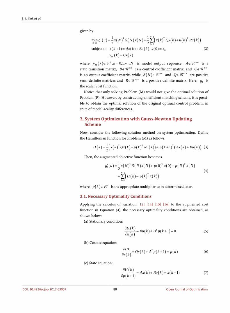
given by

( )( ) ( ) ( ) ( ) ( ) ( ) ( ) ( )( )

( ) ( ) ( ) ( )( ) ( )

1T T T1

0

0

1 1min2 2

subject to 1 , 0

N

u k k

M

g u x N S N x N x k Qx k u k Ru k

x k Ax k Bu k x x

y k Cx k

−

=

= + +

+ = + =

=

∑ (2)

where ( ) , 0,1, ,pMy k k N∈ℜ = is model output sequence, n nA ×∈ℜ is a

state transition matrix, n mB ×∈ℜ is a control coefficient matrix, and p nC ×∈ℜ is an output coefficient matrix, while ( ) n nS N ×∈ℜ and n nQ ×∈ℜ are positive semi-definite matrices and m mR ×∈ℜ is a positive definite matrix. Here, 1g is the scalar cost function.

Notice that only solving Problem (M) would not give the optimal solution of Problem (P). However, by constructing an efficient matching scheme, it is possi-ble to obtain the optimal solution of the original optimal control problem, in spite of model-reality differences.

3. System Optimization with Gauss-Newton Updating Scheme

Now, consider the following solution method on system optimization. Define the Hamiltonian function for Problem (M) as follows:

( ) ( ) ( ) ( ) ( )( ) ( ) ( ) ( )( )T T T1 12

H k x k Qx k u k Ru k p k Ax k Bu k= + + + + . (3)

Then, the augmented objective function becomes

( ) ( ) ( ) ( ) ( ) ( ) ( ) ( )

( ) ( ) ( )( )

T T T1

1 T

0

1 0 02

N

k

g u x N S N x N p x p N x N

H k p k x k−

=

′ = + −

+ −∑ (4)

where ( ) np k ∈ℜ is the appropriate multiplier to be determined later.

3.1. Necessary Optimality Conditions

Applying the calculus of variation [12] [14] [15] [16] to the augmented cost function in Equation (4), the necessary optimality conditions are obtained, as shown below:

(a) Stationary condition:

( )( ) ( ) ( )T 1 0

H kRu k B p k

u k∂

= + + =∂

(5)

(b) Costate equation:

( ) ( ) ( ) ( )T 1Hk Qx k A p k p kx k∂

= + + =∂

(6)

(c) State equation:

( )( ) ( ) ( ) ( )1

1H k

Ax k Bu k x kp k∂

= + = +∂ +

(7)

S. L. Kek et al.

DOI: 10.4236/ojop.2017.63007 89 Open Journal of Optimization

with the boundary conditions ( ) 00x x= and ( ) ( ) ( )p N S N x N= .

3.2. Feedback Optimal Control Law

According to the necessary conditions given in Equations (5) to (7), a feedback optimal control law could be constructed in which the optimal solution of Prob-lem (M) is obtained. For this purpose, the corresponding result is stated in fol-lowing theorem.

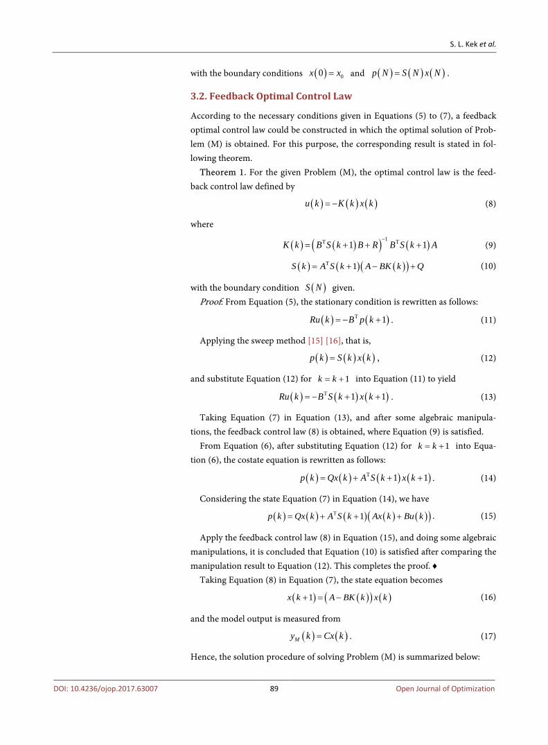
Theorem 1. For the given Problem (M), the optimal control law is the feed-back control law defined by

( ) ( ) ( )u k K k x k= − (8)

where

( ) ( )( ) ( )1T T1 1K k B S k B R B S k A−

= + + + (9)

( ) ( ) ( )( )T 1S k A S k A BK k Q= + − + (10)

with the boundary condition ( )S N given. Proof: From Equation (5), the stationary condition is rewritten as follows:

( ) ( )T 1Ru k B p k= − + . (11)

Applying the sweep method [15] [16], that is,

( ) ( ) ( )p k S k x k= , (12)

and substitute Equation (12) for 1k k= + into Equation (11) to yield

( ) ( ) ( )T 1 1Ru k B S k x k= − + + . (13)

Taking Equation (7) in Equation (13), and after some algebraic manipula-tions, the feedback control law (8) is obtained, where Equation (9) is satisfied.

From Equation (6), after substituting Equation (12) for 1k k= + into Equa-tion (6), the costate equation is rewritten as follows:

( ) ( ) ( ) ( )T 1 1p k Qx k A S k x k= + + + . (14)

Considering the state Equation (7) in Equation (14), we have

( ) ( ) ( ) ( ) ( )( )T 1p k Qx k A S k Ax k Bu k= + + + . (15)

Apply the feedback control law (8) in Equation (15), and doing some algebraic manipulations, it is concluded that Equation (10) is satisfied after comparing the manipulation result to Equation (12). This completes the proof. ♦

Taking Equation (8) in Equation (7), the state equation becomes

( ) ( )( ) ( )1x k A BK k x k+ = − (16)

and the model output is measured from

( ) ( )My k Cx k= . (17)

Hence, the solution procedure of solving Problem (M) is summarized below:

S. L. Kek et al.

DOI: 10.4236/ojop.2017.63007 90 Open Journal of Optimization

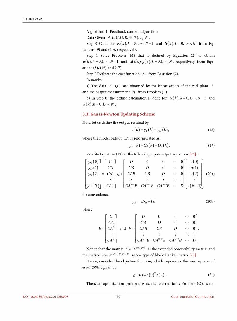
Algorithm 1: Feedback control algorithm Data Given ( ) 0, , , , , , ,A B C Q R S N x N . Step 0 Calculate ( ) , 0,1, , 1K k k N= − and ( ) , 0,1, ,S k k N= from Eq-

uations (9) and (10), respectively. Step 1 Solve Problem (M) that is defined by Equation (2) to obtain ( ) , 0,1, , 1u k k N= − and ( ) ( ), , 0,1, ,Mx k y k k N= , respectively, from Equ-

ations (8), (16) and (17). Step 2 Evaluate the cost function 1g from Equation (2). Remarks: a) The data , ,A B C are obtained by the linearization of the real plant f

and the output measurement h from Problem (P). b) In Step 0, the offline calculation is done for ( ) , 0,1, , 1K k k N= − and ( ) , 0,1, ,S k k N= .

3.3. Gauss-Newton Updating Scheme

Now, let us define the output residual by

( ) ( ) ( ) ,P Mr u y k y k= − (18)

where the model output (17) is reformulated as

( ) ( ) ( )My k Cx k Du k= + . (19)

Rewrite Equation (19) as the following input-output equations [25]:

( )( )( )

( )

( )( )( )

( )

20

1 2 3

0 00 0 01 10 02 20

1

M

M

M

N N N NM

y uC Dy uCA CB D

xy uCA CAB CB D

y N u NCA CA B CA B CA B D− − −

= + −

(20a)

for convenience,

0My Ex Fu= + (20b)

where

2

N

CCA

E CA

CA

=

and

1 2 3

0 0 00 0

0

N N N

DCB D

F CAB CB D

CA B CA B CA B D− − −

=

.

Notice that the matrix ( )1N p nE + ×∈ℜ is the extended observability matrix, and the matrix ( ) ( )1 1N p N mF + × +∈ℜ is one type of block Hankel matrix [25].

Hence, consider the objective function, which represents the sum squares of error (SSE), given by

( ) ( ) ( )T2g u r u r u= . (21)

Then, an optimization problem, which is referred to as Problem (O), is de-

S. L. Kek et al.

DOI: 10.4236/ojop.2017.63007 91 Open Journal of Optimization

fined as follows: Problem (O): Find a set of the control sequence ( ) , 0,1, , 1u k k N= − , such that the objec-

tive function 2g is minimized. To solve Problem (O), consider the second-order Taylor expansion [26] [27]

about the current ( )iu at iteration i :

( )( ) ( )( ) ( ) ( )( ) ( )( )( ) ( )( ) ( )( )( ) ( ) ( )( )

T1 12 2 2

T1 122

1 .2

i i i i i

i i i i i

g u g u u u g u

u u g u u u

+ +

+ +

≈ + − ∇

+ − ∇ − (22)

The first-order condition for Equation (22) with respect to ( )1iu + is expressed by

( )( ) ( )( )( ) ( ) ( )( )122 20 i i i ig u g u u u+≈ ∇ + ∇ − . (23)

Rearrange Equation (23) to yield the normal equation, ( )( )( ) ( ) ( )( ) ( )( )12

2 2i i i ig u u u g u+∇ − = −∇ . (24)

Notice that the gradient of 2g is calculated from ( )( ) ( )( ) ( )( )T

2 2i i ig u r u r u∇ = ∇ (25)

and the Hessian matrix of 2g is computed from

( )( ) ( )( ) ( )( ) ( )( ) ( )( )T T2 22 2i i i i ig u r u r u r u r u ∇ = ∇ +∇ ∇

(26)

where ( )( )ir u∇ is the Jacobian matrix of ( )( )ir u , and its entries are denoted by

( )( )( ) ( )( ) , 1, 2, , 1; 1,2, , 1.i ii

ij j

rr u u F i N j Nu∂

∇ = = = − = −∂

(27)

From Equations (25) and (26), Equation (24) can be rewritten as

( )( ) ( )( ) ( )( ) ( )( ) ( ) ( )( ) ( )( ) ( )( )T T T12 i i i i i i i ir u r u r u r u u u r u r u+ ∇ +∇ ∇ − = −∇

. (28)

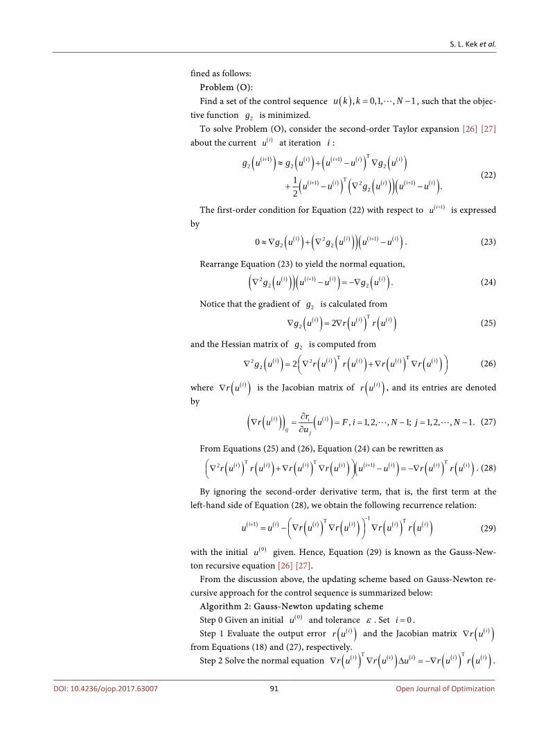
By ignoring the second-order derivative term, that is, the first term at the left-hand side of Equation (28), we obtain the following recurrence relation:

( ) ( ) ( )( ) ( )( ) ( )( ) ( )( )1T T1i i i i i iu u r u r u r u r u−

+ = − ∇ ∇ ∇

(29)

with the initial ( )0u given. Hence, Equation (29) is known as the Gauss-New- ton recursive equation [26] [27].

From the discussion above, the updating scheme based on Gauss-Newton re-cursive approach for the control sequence is summarized below:

Algorithm 2: Gauss-Newton updating scheme Step 0 Given an initial ( )0u and tolerance ε . Set 0i = . Step 1 Evaluate the output error ( )( )ir u and the Jacobian matrix ( )( )ir u∇

from Equations (18) and (27), respectively. Step 2 Solve the normal equation ( )( ) ( )( ) ( ) ( )( ) ( )( )T Ti i i i ir u r u u r u r u∇ ∇ ∆ = −∇ .

S. L. Kek et al.

DOI: 10.4236/ojop.2017.63007 92 Open Journal of Optimization

Step 3 Update the control sequence by ( ) ( ) ( )1i i iu u u+ = + ∆ . If ( ) ( )1i iu u+ = , within a given tolerance ε , stop; else set 1i i= + and repeat from Step 1 to Step 3.

Remarks: a) In Step 1, the calculation of the output error ( )( )ir u is done online, while

the Jacobian matrix ( )( )ir u∇ might be done offline. b) In Step 2, the inverse of ( )( ) ( )( )Ti ir u r u∇ ∇ must be exist. The value of ( )iu∆ represents the step-size for the control set-point.

c) In Step 3, the initial ( )0u is taken from Equation (8). The condition ( ) ( )1i iu u+ = is required to be satisfied for the converged optimal control se-

quence. The following 2-norm is computed and it is compared with a given to-lerance to verify the convergence of ( )u k :

( ) ( ) ( )( ) ( )( )1 21 11

0

N i ii i

ku u u k u k

−++

=

− = − ∑ . (30)

d) In order to provide a convergence mechanism for the state sequence, a simple relaxation method is employed:

( ) ( ) ( )( )1i i ix px x k x x+ = + − (31)

where [ ]0,1xk ∈ , px is the state sequence of the real plant and ( )ix is updated from (16).

4. Illustrative Examples

In this section, two examples are illustrated. The first example shows a direct current and alternating current (DC/AC) converter model [28] [29], while the second example gives a model of an isothermal series/parallel Van de Vussue reaction in a continuous stirred-tank reactor [30] [31]. In these models, the real plants are in nonlinear structure and the single output is measured. Since these models are in continuous time, the simple discretization scheme with the respec-tive sampling time is applied. The optimal solution would be obtained by using the approach proposed and the solution procedure is implemented in the MATLAB environment.

To be convenient, the quadratic criterion cost function, for both Problem (P) and Problem (M), is employed, that is,

( ) ( ) ( ) ( ) ( ) ( ) ( )( )1T T T

0

1 12 2

N

kx N S N x N x k Qx k u k Ru k

−

=

+ +∑

where ( ) 2 2S N I ×= , 2 2Q I ×= and 1R = .

4.1. Example 1

Consider the state space representation of a direct current/alternating current (DC/AC) converter model [28] [29] given by

( )( )( )( ) ( ) ( )

22

1 11

5 5x t

x t x t u tx t

= − +

S. L. Kek et al.

DOI: 10.4236/ojop.2017.63007 93 Open Journal of Optimization

( )( )( )( )( )

( ) ( )( ) ( ) ( )

32 2

2 2 1211

7 5 2x t x t

x t x t x t u tx tx t

= − + +

( ) ( )2y t x t=

with the initial ( )T0 0.1,0x = , where 1x and 2x represent the current (in unit

of ampere) and the voltage (in unit of volt) flow in the circuit, and u is the control signal. This problem is referred to as Problem (P).

The discrete time model of Problem (M) is formulated by

( )( )

( )( ) ( )1 1

2 2

1 1 5 0 51 0 1 7 0.2

x k x kT Tu k

x k x kT T + − ⋅ ⋅

= + + − ⋅ ⋅

( ) ( )2y k x k=

for 0,1, ,80k = , with the sampling time 0.01T = minute. The simulation result is shown in Table 1. The initial cost of 0.0429 unit,

which is the cost function value for Problem (M), is calculated before the itera-tion. After five iterations, the convergence is achieved. The final cost of 110.8926 units is preferred instead of the original cost of 1.0885 × 103 units. This reduc-tion saves 89.8 percent of the expense. The value of SSE of 7.647011 × 10–12 shows that the model output is very close to the real output. Hence, the ap-proach proposed is efficient to obtain the optimal solution of Problem (P).

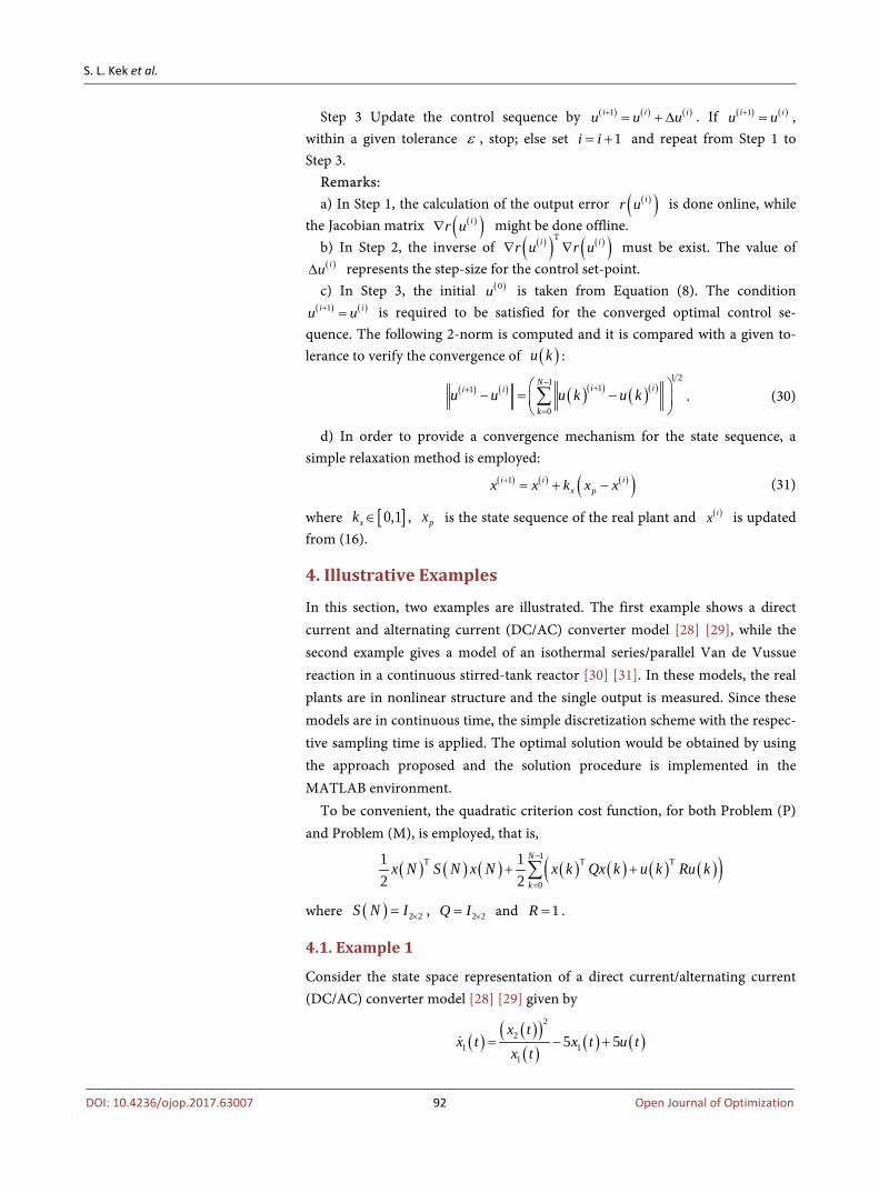
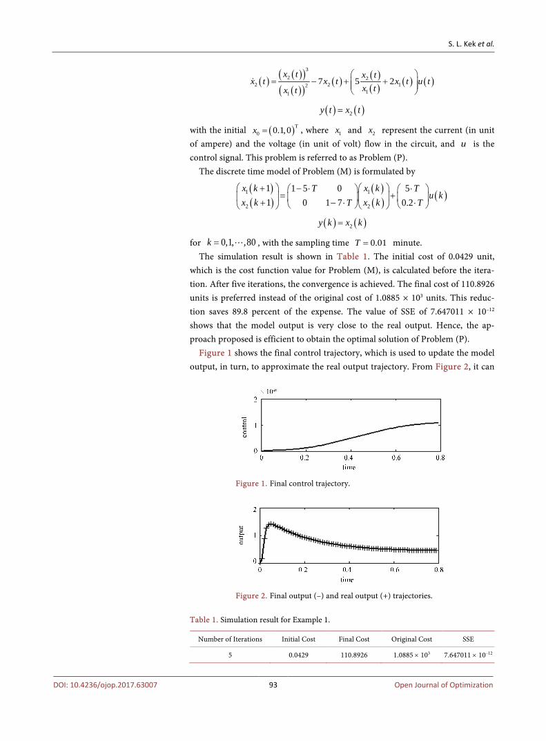
Figure 1 shows the final control trajectory, which is used to update the model output, in turn, to approximate the real output trajectory. From Figure 2, it can

Figure 1. Final control trajectory.

Figure 2. Final output (–) and real output (+) trajectories.

Table 1. Simulation result for Example 1.

Number of Iterations Initial Cost Final Cost Original Cost SSE

5 0.0429 110.8926 1.0885 × 103 7.647011 × 10–12

S. L. Kek et al.

DOI: 10.4236/ojop.2017.63007 94 Open Journal of Optimization

be seen that both of the output trajectories are fitted each other with the smallest value of SSE.

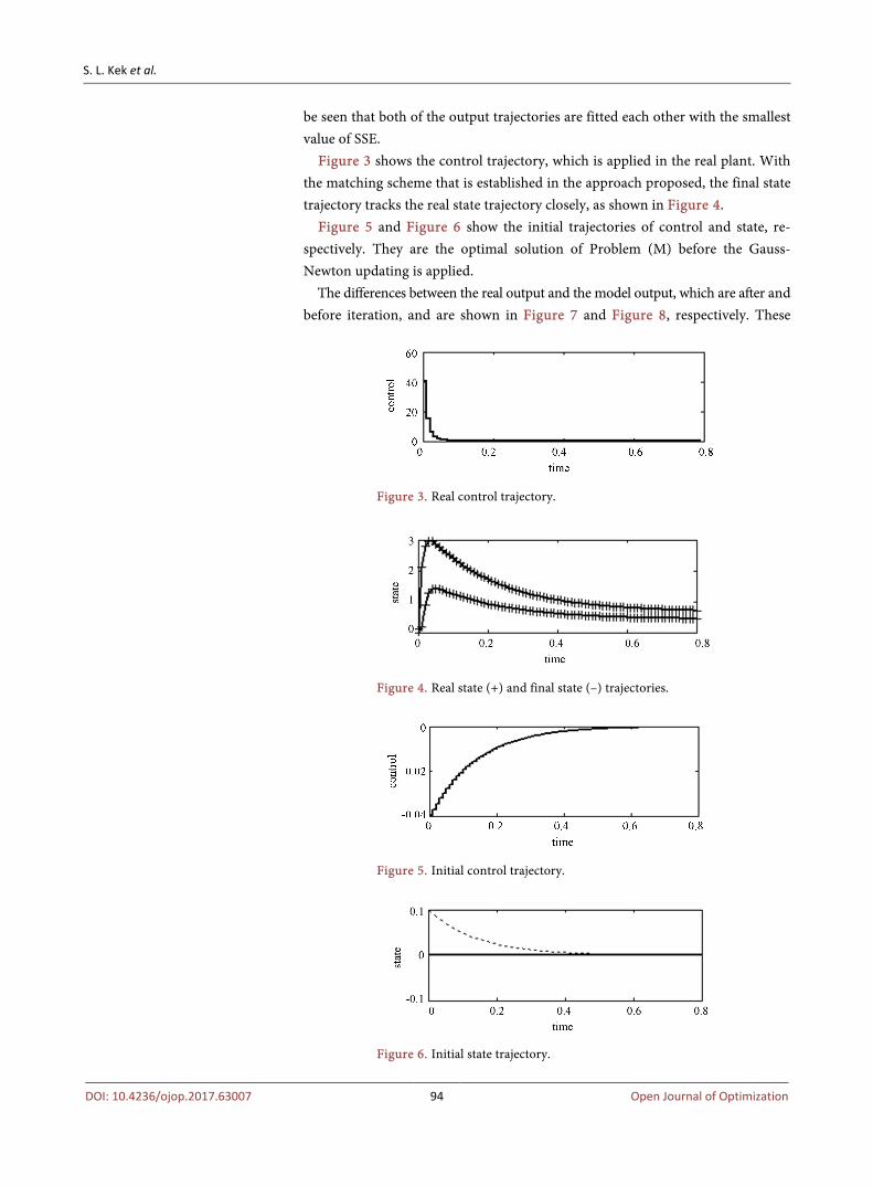
Figure 3 shows the control trajectory, which is applied in the real plant. With the matching scheme that is established in the approach proposed, the final state trajectory tracks the real state trajectory closely, as shown in Figure 4.

Figure 5 and Figure 6 show the initial trajectories of control and state, re-spectively. They are the optimal solution of Problem (M) before the Gauss- Newton updating is applied.

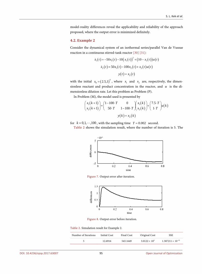
The differences between the real output and the model output, which are after and before iteration, and are shown in Figure 7 and Figure 8, respectively. These

Figure 3. Real control trajectory.

Figure 4. Real state (+) and final state (–) trajectories.

Figure 5. Initial control trajectory.

Figure 6. Initial state trajectory.

S. L. Kek et al.

DOI: 10.4236/ojop.2017.63007 95 Open Journal of Optimization

model-reality differences reveal the applicability and reliability of the approach proposed, where the output error is minimized definitely.

4.2. Example 2

Consider the dynamical system of an isothermal series/parallel Van de Vussue reaction in a continuous stirred-tank reactor [30] [31]:

( ) ( ) ( )( ) ( )( ) ( )21 1 1 150 10 10x t x t x t x t u t= − − + −

( ) ( ) ( ) ( ) ( )2 1 2 250 100x t x t x t x t u t= − +

( ) ( )2y t x t=

with the initial ( )T0 2.5,1x = , where 1x and 2x are, respectively, the dimen-

sionless reactant and product concentration in the reactor, and u is the di-mensionless dilution rate. Let this problem as Problem (P).

In Problem (M), the model used is presented by

( )( )

( )( ) ( )1 1

2 2

1 1 100 0 7.51 50 1 100 1

x k x kT Tu k

x k x kT T T + − ⋅ ⋅

= + + ⋅ − ⋅ ⋅

( ) ( )2y k x k=

for 0,1, ,100k = , with the sampling time 0.002T = second. Table 2 shows the simulation result, where the number of iteration is 5. The

Figure 7. Output error after iteration.

Figure 8. Output error before iteration.

Table 2. Simulation result for Example 2.

Number of Iterations Initial Cost Final Cost Original Cost SSE

5 12.6916 543.1649 3.0122 × 105 1.587211 × 10–12

S. L. Kek et al.

DOI: 10.4236/ojop.2017.63007 96 Open Journal of Optimization

implementation of the approach proposed begins with the initial cost of 12.6916 units. During the iterative procedure, the convergence is achieved with giving the final cost of 543.1649 units. This shows a reduction of 99.8 percent of the saving cost from the original cost of 3.0122 × 105 units. The value of SSE of 1.587211 × 10–12 indicates that the approach proposed is efficient to generate the optimal solution of Problem (P).

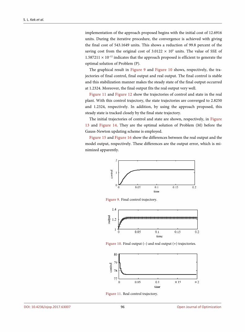
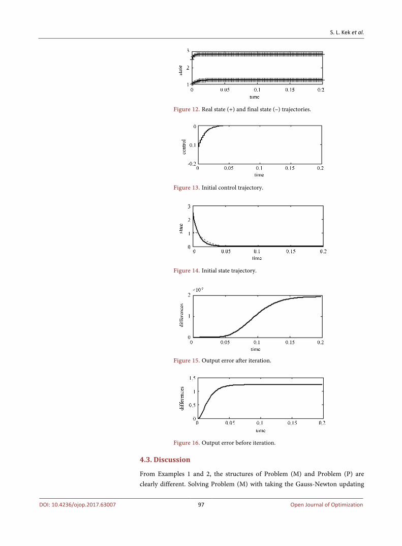
The graphical result in Figure 9 and Figure 10 shows, respectively, the tra-jectories of final control, final output and real output. The final control is stable and this stabilization manner makes the steady state of the final output occurred at 1.2324. Moreover, the final output fits the real output very well.

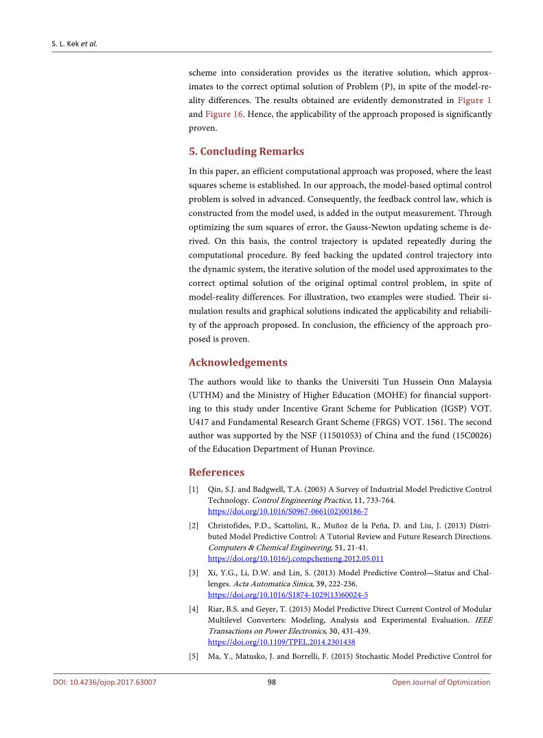
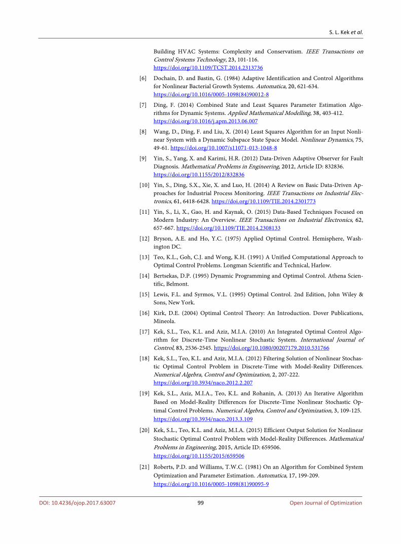
Figure 11 and Figure 12 show the trajectories of control and state in the real plant. With this control trajectory, the state trajectories are converged to 2.8250 and 1.2324, respectively. In addition, by using the approach proposed, this steady state is tracked closely by the final state trajectory.

The initial trajectories of control and state are shown, respectively, in Figure 13 and Figure 14. They are the optimal solution of Problem (M) before the Gauss-Newton updating scheme is employed.

Figure 15 and Figure 16 show the differences between the real output and the model output, respectively. These differences are the output error, which is mi-nimized apparently.

Figure 9. Final control trajectory.

Figure 10. Final output (–) and real output (+) trajectories.

Figure 11. Real control trajectory.

S. L. Kek et al.

DOI: 10.4236/ojop.2017.63007 97 Open Journal of Optimization

Figure 12. Real state (+) and final state (–) trajectories.

Figure 13. Initial control trajectory.

Figure 14. Initial state trajectory.

Figure 15. Output error after iteration.

Figure 16. Output error before iteration.

4.3. Discussion

From Examples 1 and 2, the structures of Problem (M) and Problem (P) are clearly different. Solving Problem (M) with taking the Gauss-Newton updating

S. L. Kek et al.

DOI: 10.4236/ojop.2017.63007 98 Open Journal of Optimization

scheme into consideration provides us the iterative solution, which approx-imates to the correct optimal solution of Problem (P), in spite of the model-re- ality differences. The results obtained are evidently demonstrated in Figure 1 and Figure 16. Hence, the applicability of the approach proposed is significantly proven.

5. Concluding Remarks

In this paper, an efficient computational approach was proposed, where the least squares scheme is established. In our approach, the model-based optimal control problem is solved in advanced. Consequently, the feedback control law, which is constructed from the model used, is added in the output measurement. Through optimizing the sum squares of error, the Gauss-Newton updating scheme is de-rived. On this basis, the control trajectory is updated repeatedly during the computational procedure. By feed backing the updated control trajectory into the dynamic system, the iterative solution of the model used approximates to the correct optimal solution of the original optimal control problem, in spite of model-reality differences. For illustration, two examples were studied. Their si-mulation results and graphical solutions indicated the applicability and reliabili-ty of the approach proposed. In conclusion, the efficiency of the approach pro-posed is proven.

Acknowledgements

The authors would like to thanks the Universiti Tun Hussein Onn Malaysia (UTHM) and the Ministry of Higher Education (MOHE) for financial support-ing to this study under Incentive Grant Scheme for Publication (IGSP) VOT. U417 and Fundamental Research Grant Scheme (FRGS) VOT. 1561. The second author was supported by the NSF (11501053) of China and the fund (15C0026) of the Education Department of Hunan Province.

References [1] Qin, S.J. and Badgwell, T.A. (2003) A Survey of Industrial Model Predictive Control

Technology. Control Engineering Practice, 11, 733-764. https://doi.org/10.1016/S0967-0661(02)00186-7

[2] Christofides, P.D., Scattolini, R., Muñoz de la Peña, D. and Liu, J. (2013) Distri-buted Model Predictive Control: A Tutorial Review and Future Research Directions. Computers & Chemical Engineering, 51, 21-41. https://doi.org/10.1016/j.compchemeng.2012.05.011

[3] Xi, Y.G., Li, D.W. and Lin, S. (2013) Model Predictive Control—Status and Chal-lenges. Acta Automatica Sinica, 39, 222-236. https://doi.org/10.1016/S1874-1029(13)60024-5

[4] Riar, B.S. and Geyer, T. (2015) Model Predictive Direct Current Control of Modular Multilevel Converters: Modeling, Analysis and Experimental Evaluation. IEEE Transactions on Power Electronics, 30, 431-439. https://doi.org/10.1109/TPEL.2014.2301438

[5] Ma, Y., Matusko, J. and Borrelli, F. (2015) Stochastic Model Predictive Control for

S. L. Kek et al.

DOI: 10.4236/ojop.2017.63007 99 Open Journal of Optimization

Building HVAC Systems: Complexity and Conservatism. IEEE Transactions on Control Systems Technology, 23, 101-116. https://doi.org/10.1109/TCST.2014.2313736

[6] Dochain, D. and Bastin, G. (1984) Adaptive Identification and Control Algorithms for Nonlinear Bacterial Growth Systems. Automatica, 20, 621-634. https://doi.org/10.1016/0005-1098(84)90012-8

[7] Ding, F. (2014) Combined State and Least Squares Parameter Estimation Algo-rithms for Dynamic Systems. Applied Mathematical Modelling, 38, 403-412. https://doi.org/10.1016/j.apm.2013.06.007

[8] Wang, D., Ding, F. and Liu, X. (2014) Least Squares Algorithm for an Input Nonli-near System with a Dynamic Subspace State Space Model. Nonlinear Dynamics, 75, 49-61. https://doi.org/10.1007/s11071-013-1048-8

[9] Yin, S., Yang, X. and Karimi, H.R. (2012) Data-Driven Adaptive Observer for Fault Diagnosis. Mathematical Problems in Engineering, 2012, Article ID: 832836. https://doi.org/10.1155/2012/832836

[10] Yin, S., Ding, S.X., Xie, X. and Luo, H. (2014) A Review on Basic Data-Driven Ap-proaches for Industrial Process Monitoring. IEEE Transactions on Industrial Elec-tronics, 61, 6418-6428. https://doi.org/10.1109/TIE.2014.2301773

[11] Yin, S., Li, X., Gao, H. and Kaynak, O. (2015) Data-Based Techniques Focused on Modern Industry: An Overview. IEEE Transactions on Industrial Electronics, 62, 657-667. https://doi.org/10.1109/TIE.2014.2308133

[12] Bryson, A.E. and Ho, Y.C. (1975) Applied Optimal Control. Hemisphere, Wash-ington DC.

[13] Teo, K.L., Goh, C.J. and Wong, K.H. (1991) A Unified Computational Approach to Optimal Control Problems. Longman Scientific and Technical, Harlow.

[14] Bertsekas, D.P. (1995) Dynamic Programming and Optimal Control. Athena Scien-tific, Belmont.

[15] Lewis, F.L. and Syrmos, V.L. (1995) Optimal Control. 2nd Edition, John Wiley & Sons, New York.

[16] Kirk, D.E. (2004) Optimal Control Theory: An Introduction. Dover Publications, Mineola.

[17] Kek, S.L., Teo, K.L. and Aziz, M.I.A. (2010) An Integrated Optimal Control Algo-rithm for Discrete-Time Nonlinear Stochastic System. International Journal of Control, 83, 2536-2545. https://doi.org/10.1080/00207179.2010.531766

[18] Kek, S.L., Teo, K.L. and Aziz, M.I.A. (2012) Filtering Solution of Nonlinear Stochas-tic Optimal Control Problem in Discrete-Time with Model-Reality Differences. Numerical Algebra, Control and Optimization, 2, 207-222. https://doi.org/10.3934/naco.2012.2.207

[19] Kek, S.L., Aziz, M.I.A., Teo, K.L. and Rohanin, A. (2013) An Iterative Algorithm Based on Model-Reality Differences for Discrete-Time Nonlinear Stochastic Op-timal Control Problems. Numerical Algebra, Control and Optimization, 3, 109-125. https://doi.org/10.3934/naco.2013.3.109

[20] Kek, S.L., Teo, K.L. and Aziz, M.I.A. (2015) Efficient Output Solution for Nonlinear Stochastic Optimal Control Problem with Model-Reality Differences. Mathematical Problems in Engineering, 2015, Article ID: 659506. https://doi.org/10.1155/2015/659506

[21] Roberts, P.D. and Williams, T.W.C. (1981) On an Algorithm for Combined System Optimization and Parameter Estimation. Automatica, 17, 199-209. https://doi.org/10.1016/0005-1098(81)90095-9

S. L. Kek et al.

DOI: 10.4236/ojop.2017.63007 100 Open Journal of Optimization

[22] Roberts, P.D. (1992) Optimal Control of Nonlinear Systems with Model-Reality Differences. Proceedings of the 31st IEEE Conference on Decision and Control, 1, 257-258. https://doi.org/10.1109/CDC.1992.371744

[23] Becerra, V.M. and Roberts, P.D. (1996) Dynamic Integrated System Optimization and Parameter Estimation for Discrete-Time Optimal Control of Nonlinear Sys-tems. International Journal of Control, 63, 257-281. https://doi.org/10.1080/00207179608921843

[24] Kek, S.L., Li, J. and Teo, K.L. (2017) Least Square Solution for Discrete Time Non-linear Stochastic Optimal Control Problem with Model-Reality Differences. Applied Mathematics, 8, 1-14. https://doi.org/10.4236/am.2017.81001

[25] Verhaegen, M. and Verdult, V. (2007) Filtering and System Identification: A Least Squares Approach. Cambridge University Press, Cambridge. https://doi.org/10.1017/CBO9780511618888

[26] Minoux, M. (1986) Mathematical Programming Theory and Algorithms. John Wi-ley & Sons, New York.

[27] Chong, E.K.P. and Zak, S.H. (2013) An Introduction to Optimization. 4th Edition, John Wiley & Sons, New York.

[28] Poursafar, N., Taghirad, H.D. and Haeri, M. (2010) Model Predictive Control of Nonlinear Discrete-Time Systems: A Linear Matrix Inequality Approach. IET Con-trol Theory and Applications, 4, 1922-1932. https://doi.org/10.1049/iet-cta.2009.0650

[29] Haeri, M. (2004) Improved EDMC for the Processes with High Variations and/or Sign Changes in Steady-State Gain. COMPEL: International Journal of Computa-tions & Mathematics in Electrical, 23, 361-380. https://doi.org/10.1108/03321640410510541

[30] Shridhar, R. and Cooper, D.J. (1997) A Tuning Strategy for Unconstrained SISO Model Predictive Control. Industrial & Engineering Chemistry Research, 36, 729- 746. https://doi.org/10.1021/ie9604280

[31] Kravaris, C. and Daoutidis, P. (1990) Nonlinear State-Feedback Control of Second Order Non-Minimum Phase Systems. Computers & Chemical Engineering, 14, 439- 449. https://doi.org/10.1016/0098-1354(90)87019-L

Submit or recommend next manuscript to SCIRP and we will provide best service for you:

Accepting pre-submission inquiries through Email, Facebook, LinkedIn, Twitter, etc. A wide selection of journals (inclusive of 9 subjects, more than 200 journals) Providing 24-hour high-quality service User-friendly online submission system Fair and swift peer-review system Efficient typesetting and proofreading procedure Display of the result of downloads and visits, as well as the number of cited articles Maximum dissemination of your research work

Submit your manuscript at: http://papersubmission.scirp.org/ Or contact ojop@scirp.org