A Game Theoretical Approach to Communication Security
125
A Game Theoretical Approach to Communication Security Assane Gueye Electrical Engineering and Computer Sciences University of California at Berkeley Technical Report No. UCB/EECS-2011-19 http://www.eecs.berkeley.edu/Pubs/TechRpts/2011/EECS-2011-19.html March 14, 2011
-
Upload
phungtuyen -
Category
Documents
-
view
228 -
download
1
Transcript of A Game Theoretical Approach to Communication Security

A Game Theoretical Approach to Communication Security
Assane Gueye
Electrical Engineering and Computer SciencesUniversity of California at Berkeley
Technical Report No. UCB/EECS-2011-19
http://www.eecs.berkeley.edu/Pubs/TechRpts/2011/EECS-2011-19.html
March 14, 2011

Copyright © 2011, by the author(s).All rights reserved.
Permission to make digital or hard copies of all or part of this work forpersonal or classroom use is granted without fee provided that copies arenot made or distributed for profit or commercial advantage and that copiesbear this notice and the full citation on the first page. To copy otherwise, torepublish, to post on servers or to redistribute to lists, requires prior specificpermission.
Acknowledgement
I would like to thank my adviser Prof. Jean Walrand and all my dissertationcommittee members.Thanks to my parents for all they have done for me.
A Game Theoretical Approach to Communication Security
by
Assane Gueye
A dissertation submitted in partial satisfaction of the
requirements for the degree of
Doctor of Philosophy
in
Engineering–Electrical Engineering and Computer Sciences
in the
Graduate Division
of the
University of California, Berkeley
Committee in charge:
Professor Jean C. Walrand, ChairProfessor Venkat Anantharam
Professor Shachar KarivProfessor Vern Paxson
Spring 2011

A Game Theoretical Approach to Communication Security
Copyright 2011
by
Assane Gueye
1
Abstract
A Game Theoretical Approach to Communication Security
by
Assane Gueye
Doctor of Philosophy in Engineering–Electrical Engineering and Computer Sciences
University of California, Berkeley
Professor Jean C. Walrand, Chair
The increased reliance on the Internet has made information and communication systems morevulnerable to security attacks. Many recent incidents demonstrate this vulnerability, such as therapid propagation of sophisticated malwares, the fast growth of botnets, denial-of-service (DoS)attacks against business and government websites, and attacks against the power grid system.
Experts must design and implement security solutions to defend against well organized and verysophisticated adversaries such as malicious insiders, cybercriminals, cyberterrorists, industrial spies,and, in some cases, nation-state intelligence agents.
Instead of designing a defense against a specific attack, Game Theory attempts to design a defenseagainst a sophisticated attacker who plans in anticipation of a complex defense. By includingthis ‘second-guessing’ element into the design process, Game Theory has the potential of craftingimproved security mechanisms. In addition, Game Theory can model issues of trust, incentives,and externalities that arise in security systems.
This thesis illustrates the potential usefulness of Game Theory in security. By modeling theinteractions between defenders and attackers as games in three types of common communicationscenarios, we predict the adversaries’ attacks, determine the set of assets that are most likely to beattacked, and suggest defense strategies for the defenders.
The first example is a communication scenario where some components might be compromised.Specifically, we consider Bob who is receiving information that might be corrupted by an attacker,Trudy. We model the interaction between Trudy and Bob as a zero-sum game where Trudy chooseswhether and how to corrupt the data and Bob decides how much he should trust the receivedinformation. By analyzing the Nash equilibrium of the game, we have determined when Bob shouldtrust the received information, and how Trudy should corrupt the data. We have also shown howa challenge-response option for Bob can deter Trudy from corrupting the information.

2
The second example is a scenario where an intelligent virus is attempting to infect a networkprotected by an Intrusion Detection System (IDS). The IDS detects intrusions by analyzing thevolume of traffic going inside the network. We model the interaction of the intelligent virus and theIDS as a zero-sum game where the IDS chooses the detection threshold, while the virus is tryingto choose its infection rate to maximize its ultimate spreading. Using a Markov chain model, wecompute the Nash equilibria of the game and analyze them. In general, a more aggressive virus ismore damaging but is also faster to detect. Hence, in its best attack, the intelligent virus choosesan infection rate that balances between an aggressive attack that can be easily detected and a slowattack that causes less damage. The best defense strategy against such a sophisticated virus is toquarantine the traffic and analyze it prior to letting it go inside the network (in addition to settingthe optimal threshold).
The third example is a blocking security game. For this game, given a finite set of resourcesE = e1, . . . , em, a defender needs to choose a feasible subset T ⊆ E of resources to perform amission critical task. The attacker, at the same time, tries to disrupt the task by choosing oneresource e ∈ E to attack. Each resource e ∈ E has a cost of attack µe. The defender loses somevalue λT,e whenever the task is disrupted (i.e. the attacked resource e belongs to his subset T ).This loss goes to the attacker. We analyze the game by using the combinatorial tools of blockingpairs of matrices (hence the name blocking security game). We introduce the notion of criticalsubset of resources and use this notion to define a vulnerability metric for the task. We find that,in Nash equilibrium, the attacker always targets a critical set of resources and the defender choosesa feasible subset that minimally intersects that critical subset. We illustrate the model with twoexamples of communication scenarios that consider design of network topology in the presence ofa strategic adversary. The first example studies a scenario where a network manager is choosinga spanning tree of a graph while an attacker is trying to cut the tree by attacking one link ofthe graph. One of our findings in this scenario is that, the usual edge-connectivity metric for agraph is not the appropriate vulnerability measure in a network where strategic adversaries arepresent. The second example deals with a supply-demand network where a network manager ischoosing a feasible flow to transport the maximum amount of goods from a set of sources to a setof destinations, and an attacker is trying to minimize this by attacking an arc of the network. Inthis case, we find that critical subsets of links are cutsets that maximize the minimum fraction ofgoods carried per link of the cutset. In most cases, these correspond to minimum cutsets of thegraph.
Although computing Nash equilibria of a two-player game is generally complex, we have shownhow, for a class of blocking games, one can compute a critical set of resources (hence a Nashequilibrium) in polynomial time.

i
To my parents, my family, my wife, my son, my friends...
To my late mother...who did not live long enough to witness this moment...
Black woman, African woman,O mother, I think of you...
O Daman, O mother,Who carried me on your back, who nursed me,
Who governed my first steps,Who was the first to open my eyes to the beauties of the world,
I think of you...
Woman of the fields, woman of the rivers, woman of the great river,O mother, I think of you...
O Daman, O mother, who wiped my tears,Who cheered up my heart, who patiently dealt with my caprices,How I would love to still be near you, be a child next to you.
Simple woman, woman of resignation,O mother, my thoughts are always of you.
O Daman, Daman of the great family of true believers,My thoughts are always of you,
They accompany me with every step, O Daman, my mother,How I would love to still feel your warmth,
Be a child next to you.
Black woman, African woman,O mother, thank you; thank you for all that you have done for me, your son,
So far away yet so close to you!
Translated from the original French text of Camara LAYEby Deborah Weagel, University of New Mexico

ii
Contents
Contents ii
List of Figures vi
List of Tables ix
Acknowledgements x
1 Introduction 1
1.1 Some security incidents . . . . . . . . . . . . . . . . . . . . . . . . . . . . . . . . . . 1
1.2 Information and communication systems’ security challenges . . . . . . . . . . . . . . 2
1.2.1 Strategic and sophisticated adversaries . . . . . . . . . . . . . . . . . . . . . . 2
1.2.2 Complexity and interconnectedness . . . . . . . . . . . . . . . . . . . . . . . . 3
1.2.3 Presence of compromised and/or malicious agents and components . . . . . . 4
1.2.4 Human factors! . . . . . . . . . . . . . . . . . . . . . . . . . . . . . . . . . . . 4
1.2.5 Risk assessment and Management . . . . . . . . . . . . . . . . . . . . . . . . 5
1.3 Security solutions . . . . . . . . . . . . . . . . . . . . . . . . . . . . . . . . . . . . . . 6
1.3.1 Practical security solutions . . . . . . . . . . . . . . . . . . . . . . . . . . . . 6
1.3.2 Analytical approaches . . . . . . . . . . . . . . . . . . . . . . . . . . . . . . . 7
1.4 Game Theory Potentials . . . . . . . . . . . . . . . . . . . . . . . . . . . . . . . . . . 7
1.5 Thesis summary . . . . . . . . . . . . . . . . . . . . . . . . . . . . . . . . . . . . . . 9
1.5.1 Communication security games . . . . . . . . . . . . . . . . . . . . . . . . . . 9
iii
1.5.2 Chapter 2: The intruder game . . . . . . . . . . . . . . . . . . . . . . . . . . 10
1.5.3 Chapter 3: The intelligent virus game . . . . . . . . . . . . . . . . . . . . . . 10
1.5.4 Chapter 4: Blocking games . . . . . . . . . . . . . . . . . . . . . . . . . . . . 11
1.5.5 Challenges to applying Game Theory to security . . . . . . . . . . . . . . . . 12
1.6 Game Theory basics . . . . . . . . . . . . . . . . . . . . . . . . . . . . . . . . . . . . 12
1.7 Related work . . . . . . . . . . . . . . . . . . . . . . . . . . . . . . . . . . . . . . . . 15
2 Intruder Game 19
2.1 Simple Intruder Game . . . . . . . . . . . . . . . . . . . . . . . . . . . . . . . . . . . 20
2.2 Nash Equilibrium . . . . . . . . . . . . . . . . . . . . . . . . . . . . . . . . . . . . . . 21
2.2.1 Understanding the NE . . . . . . . . . . . . . . . . . . . . . . . . . . . . . . . 21
2.2.2 Proof of theorem 1 . . . . . . . . . . . . . . . . . . . . . . . . . . . . . . . . . 22
2.3 Challenging the Message . . . . . . . . . . . . . . . . . . . . . . . . . . . . . . . . . . 24
2.3.1 Understanding the NE . . . . . . . . . . . . . . . . . . . . . . . . . . . . . . . 25
2.3.2 Proof of theorem 2 . . . . . . . . . . . . . . . . . . . . . . . . . . . . . . . . . 27
3 Intelligent Virus Game 32
3.1 The Intelligent Virus Game . . . . . . . . . . . . . . . . . . . . . . . . . . . . . . . . 33
3.1.1 Deriving the NE . . . . . . . . . . . . . . . . . . . . . . . . . . . . . . . . . . 34
3.1.2 Qualitative Comparison . . . . . . . . . . . . . . . . . . . . . . . . . . . . . . 35
4 Blocking Games 37
4.1 Blocking Pair of Matrices . . . . . . . . . . . . . . . . . . . . . . . . . . . . . . . . . 39
4.2 Game Model . . . . . . . . . . . . . . . . . . . . . . . . . . . . . . . . . . . . . . . . 41
4.3 Nash Equilibrium Theorem . . . . . . . . . . . . . . . . . . . . . . . . . . . . . . . . 43
4.4 Examples . . . . . . . . . . . . . . . . . . . . . . . . . . . . . . . . . . . . . . . . . . 44
4.4.1 The spanning tree – link game . . . . . . . . . . . . . . . . . . . . . . . . . . 44
The spanning tree polyhedron PΛ and its blocker bl(PΛ) . . . . . . . . . . . . 45
From feasible partitions to feasible subsets of edges . . . . . . . . . . . . . . . 48
iv
Applying the model . . . . . . . . . . . . . . . . . . . . . . . . . . . . . . . . 49
Some examples of graph . . . . . . . . . . . . . . . . . . . . . . . . . . . . . . 51
Nash equilibrium theorem applied to the spanning tree game . . . . . . . . . 52
Analyzing the NE: case µ = 0 . . . . . . . . . . . . . . . . . . . . . . . . . . . 53
Analyzing the NE: case µ > 0 . . . . . . . . . . . . . . . . . . . . . . . . . . . 55
4.4.2 Examples 2: Un-capacitated supply demand networks . . . . . . . . . . . . . 58
The Flow polyhedron PF and its blocker bl(PF ) . . . . . . . . . . . . . . . . 60
Applying the model . . . . . . . . . . . . . . . . . . . . . . . . . . . . . . . . 61
Nash equilibrium theorem for the supply-demand network game . . . . . . . 62
Examples and discussions: case case µ = 0 . . . . . . . . . . . . . . . . . . . 64
Examples and discussions: case case µ > 0 . . . . . . . . . . . . . . . . . . . 66
4.5 Proof of the NE Theorem . . . . . . . . . . . . . . . . . . . . . . . . . . . . . . . . . 67
4.5.1 “No Attack” Option . . . . . . . . . . . . . . . . . . . . . . . . . . . . . . . . 67
Best Responses . . . . . . . . . . . . . . . . . . . . . . . . . . . . . . . . . . . 67
Existence of the Equilibrium Distribution α . . . . . . . . . . . . . . . . . . . 67
4.5.2 The “Always Attack” option . . . . . . . . . . . . . . . . . . . . . . . . . . . 69
Best Responses . . . . . . . . . . . . . . . . . . . . . . . . . . . . . . . . . . . 70
Existence of the Equilibrium Distribution α . . . . . . . . . . . . . . . . . . . 72
4.5.3 Enumerating all Nash Equilibria . . . . . . . . . . . . . . . . . . . . . . . . . 75
Proof of Lemma 6 . . . . . . . . . . . . . . . . . . . . . . . . . . . . . . . . . 78
4.6 Algorithm to Compute θ and a Critical Vertex . . . . . . . . . . . . . . . . . . . . . 80
4.6.1 Deriving an algorithm . . . . . . . . . . . . . . . . . . . . . . . . . . . . . . . 81
4.6.2 Computing critical subset of edges of a graph . . . . . . . . . . . . . . . . . . 83
Polymatroids . . . . . . . . . . . . . . . . . . . . . . . . . . . . . . . . . . . . 83
Cunningham’s algorithm . . . . . . . . . . . . . . . . . . . . . . . . . . . . . . 85
Network Flow . . . . . . . . . . . . . . . . . . . . . . . . . . . . . . . . . . . . 86
5 Conclusion and Future Work 89
v
5.1 Conclusion . . . . . . . . . . . . . . . . . . . . . . . . . . . . . . . . . . . . . . . . . 89
5.1.1 Discussion: Challenges for Game Theoretic Approaches to Security . . . . . . 90
5.1.2 Experimental Design . . . . . . . . . . . . . . . . . . . . . . . . . . . . . . . . 92
Bibliography 93
A Computing Critical Subsets 100
A.1 A binary search algorithm for computing a critical subset and θ . . . . . . . . . . . . 100
A.2 Argument for Remark in Section 4.4.1 . . . . . . . . . . . . . . . . . . . . . . . . . . 101
B Experimental Study 104
B.1 Motivations . . . . . . . . . . . . . . . . . . . . . . . . . . . . . . . . . . . . . . . . . 104
B.2 Game 1 . . . . . . . . . . . . . . . . . . . . . . . . . . . . . . . . . . . . . . . . . . . 106
B.3 Game 2 . . . . . . . . . . . . . . . . . . . . . . . . . . . . . . . . . . . . . . . . . . . 106
B.4 Games 3,4,5 . . . . . . . . . . . . . . . . . . . . . . . . . . . . . . . . . . . . . . . . . 107

vi
List of Figures
2.1 Intruder game model. Alice sends a message to Bob. The message might transit viaan attacker: Trudy. The game is between Bob who wants to correctly detect themessage and Trudy who wants to corrupt it. . . . . . . . . . . . . . . . . . . . . . . . 20
2.2 The Nash Equilibria of the Intruder Game. The figures in the right show the regionsP1 and P2. . . . . . . . . . . . . . . . . . . . . . . . . . . . . . . . . . . . . . . . . . 22
2.3 The Intruder Game with Challenge. . . . . . . . . . . . . . . . . . . . . . . . . . . . 24
2.4 The Nash equilibria decision regions of the Intruder Game with challenge. . . . . . . 26
3.1 Intelligent virus game model. . . . . . . . . . . . . . . . . . . . . . . . . . . . . . . . 32
3.2 Markov chain model for computing the NE of the intelligent virus game with bufferingIDS. . . . . . . . . . . . . . . . . . . . . . . . . . . . . . . . . . . . . . . . . . . . . . 33
3.3 Cost of security as a function of the virus propagation rate. Different plots are shownfor different values of the rate of normal traffic α. . . . . . . . . . . . . . . . . . . . . 36
4.1 Example of polyhedron PΛ defined by a nonnegative proper matrix Λ and its corre-sponding blocker bl(PΛ). The extreme points of the blocker define the nonnegativeproper matrix Ω. . . . . . . . . . . . . . . . . . . . . . . . . . . . . . . . . . . . . . . 39
4.2 Examples of feasible and not feasible subsets of links. The chosen subset is shownin dashed line. The two subsets in the left are not feasible, the two subsets in theright are feasible. . . . . . . . . . . . . . . . . . . . . . . . . . . . . . . . . . . . . . . 48
4.3 Illustrative network examples where the attack cost µ = 0. Example 4.3(a) is anetwork that contains a bridge. A bridge is always a critical set. The network in4.3(b) is an example of graph where the minimum cutset (links 6,8) corresponds toa critical subset. Example 4.3(c) shows a graph where the minimum cutset is notcritical. . . . . . . . . . . . . . . . . . . . . . . . . . . . . . . . . . . . . . . . . . . . 51

vii
4.4 Illustrative network examples for µ > 0. Example 4.4(a) is a network that containsa bridge. The vector of attack costs is µ = [0.5, 0.5, 0.5, 2, 0.5, 0.5, 0.5]. There are 2critical sets: E1 = 1, 2, 3 and E2 = 5, 6, 7. The bridge is neither critical nor itdoes belong to a critical subset. In the network in 4.4(b) the vector attack costs isµ = [5, 3, 3, 5, 5, 4, 3, 3, 5, 5, 4, 5, 5, 3]/14. In this case the minimum cutset (links 6,8)corresponds to a critical subset. Example 4.4(c) shows a graph where the minimumcutset is not critical. In this case µ = [2, 5, 1, 2, 1, 1, 6, 5, 3, 7, 1, 4, 3, 6]/21. . . . . . . . 52
4.5 Critical subset and topology design. Graphs (b) and (c) are two different ways ofadding a link to graph (a) which have a vulnerability of 3/4. If it is added as in (b),then the vulnerability is 3
5 . If it is done as in (c), the vulnerability is 23 > 3
5 , whichis leads to a less robust network. . . . . . . . . . . . . . . . . . . . . . . . . . . . . . 54
4.6 Example of graph and its spanning trees. The left figure is the original graph withthe 5 edges labeled with their number. The right figures are the 8 spanning trees ofthe graph also labeled with their numbers. In the payoff column, L is the defender’sloss while R is the attacker’s reward. . . . . . . . . . . . . . . . . . . . . . . . . . . . 56
4.7 A demand-supply network. Sources S = S1, S2 produces 5 units of goods. Desti-nations T = T1, T2 needs 5 units of good. The amount of goods produced by thesources (S1, S2) is (2, 3). The destination nodes (T1, T2) need (4, 1). An example offeasible flow is shown in the figure with the amount of goods carried by each arc isthe value marked on the arcs. . . . . . . . . . . . . . . . . . . . . . . . . . . . . . . 58
4.8 Illustrative demand-supply network examples. For each graph, a feasible flow is givenby the values on the arcs. The arcs (X, X) corresponding to critical subset X, arethe dashed (dash-dotted) lines. . . . . . . . . . . . . . . . . . . . . . . . . . . . . . . 63
4.9 Illustrative demand-supply network examples for µ > 0. For each graph, the value ofthe attack cost is marked close to the arc. The arcs (X, X) corresponding to criticalsubset X, are the dashed (dash-dotted) lines. . . . . . . . . . . . . . . . . . . . . . . 68
4.10 Constructing the graph G′ for the network flow algorithm. Figure 4.10(a) shows theconstruction of G′ from G. The edge under consideration in this example is e = 5.Examples in Figures 4.10(b) show the cut induced by B ∪ r for B ⊆ V. In theleft figure, B = a, b does not contain j = 5. The capacity of this cut is equal toinfinity. In the right figure, B = a, c which contains edge e = 5 (the only edge).As can be seen in the figure, the capacity of the cut induced by this choice of B is2 + x(1) + x(2) + x(3) + x(4) which is finite. . . . . . . . . . . . . . . . . . . . . . . 88
A.1 An illustration of the 2-dimensional search algorithm to find the vulnerability of agraph. The dark (blue) region consists of p and q verifying p/q > 1. Since θ ≤ 1,those values do not need to be tested. The light (blue) consist of values of p and qsuch that p
q > p0
q0(here p0
q0= 4
7). If θ < p0
q0, then, those values can be discarded from
the test. The remaining (uncolored) values are the only ones that need to be tested. 101

viii
B.1 Example of network graph. The bold lines show one way to connect all nodes in thegraph without loop. . . . . . . . . . . . . . . . . . . . . . . . . . . . . . . . . . . . . 104
B.2 Networks considered in experiments 1 (B.2(a)) and 2 (B.2(b)). . . . . . . . . . . . . 106

ix
List of Tables
2.1 Nash equilibria strategies for the Intruder Game with challenge. . . . . . . . . . . . . 26
3.1 Values of the false alarm p0 and detection p1 probabilities. . . . . . . . . . . . . . . . 34
3.2 Nash equilibrium (β, x) as a function of the parameters (q, γ). . . . . . . . . . . . . . 35
4.1 Game with positive attack cost played for different values of the cost of attack µ. . . 56
4.2 Pseudocode: algorithm computing the value θ of the game and a critical vertex. Thealgorithm CunninghamMin is used to perform the minimization in 4.180. It returnsθ and a minimizing subset ωo . . . . . . . . . . . . . . . . . . . . . . . . . . . . . . . 81
4.3 Pseudocode of the oracle CunninghamMin that solves the minimization (4.200). . . . 86
A.1 BinarySearch2D algorithm to compute θ and a critical subset. Algorithm Cunning-hamMin is discussed in section 4.6.2. Method update method is presented in TableA.2. . . . . . . . . . . . . . . . . . . . . . . . . . . . . . . . . . . . . . . . . . . . . . 102
A.2 Pseudocode of the Update method used in the BinarySearch2D algorithm. . . . . . . 102

x
Acknowledgments
First, I thank The Lord who has given me life, health, and countless blessings. He has providedme with the strength to go through with this experience for the past 6 years and I would like topraise Him and thank Him.
I am heartily thankful to my supervisor Prof. Jean Walrand for his encouragement, guidance,support, and patience. A student’s life does not end on campus and Jean’s support has reachedme far beyond the Berkeley halls and conference rooms. Thank you for all you have done for meJean, and thanks to your family who has joined you in that.
Prof. Venkat Anantharam has generously given me his time and expertise at a crucial time ofthis dissertation. Without Venkat’s help, finishing this thesis would have been a lot more difficult.I would like to show him my endless gratitude.
I am grateful to Prof. Vern Paxson for his valuable feedback, his input, his guidance, and hiskindness. Prof. Paxson’s sound understanding of the security problem has made me love thesubject after I took his class. Thank you for all the efforts you have spent in teaching us this veryimportant subject.
I am very thankful to Prof. Shachar Kariv who has guided my steps in Game Theory and has,from the initial to the final level, enabled me to develop a good understanding of the subject.Thank you for your patience, your kindness, and your feedback.
I would like to show my gratitude to all the professors who have taught me. Also, many thanksto the entire Berkeley NetEcon group. John, Shyam, Abhay, Nikhil, Libin, Jiwoong, Galina, David,Barlas, Vijay, your suggestions and feedback were very valuable to me.
My endless thanks go to Prof. Eric Brewer and the TIER group who have supported my researchon Information and Communication Technologies for Development (ICT4D). Your devotion tobringing technologies to people in the less developed nations is noble and has inspired me a lot. Iwould specially like to thank George Sharffenberger and Scott McNeil for their guidance and manysuggestions.
I need to express my deep gratitude to Daniel Mouen-Makoua and the Gateway Foundation fortheir financial support. Daniel did not only provide finance, he has been a friend and a mentor tome. Thank you for that. Also, I must acknowledge Ambassador Martin Brennan, Josiane Siegfriedand the entire International House board for having given me the opportunity to live in such awonderful environment. Thanks to Martin for his kindness and thanks to all the friends I have metat I-House.
My thanks must go to all my friends who have helped me maintain a balanced on-campus/off-campus life. Especially, I need to express my deepest gratitude to the members of the DahiratoulTayssiroul Assir, Touba-Oakland. They have helped me develop an enriching spiritual life andhave supported me every time I needed them. Many thanks to Khadim, Lahad, and Issa whohave welcomed me to the Bay Area and have introduced me to this great community. I am always

xi
grateful to my spiritual guides Serigne Amsatou Mbacke and Serigne Khalifa Diop for their guidanceand prayers.
I am forever grateful to my family for their unconditional love and support. My parents havegiven me the best of everything in this world, they have made endless sacrifices for my educationand my success, and they have taught me and raised me to always be a good person. I certainlycannot thank them enough.
Last but not least, endless thanks to my wife for her love, care, and patience for all those longyears that I have been away from her. Thank you for taking care of our beloved son while I wasfinalizing this dissertation.

xii

1
Chapter 1
Introduction
“The art of war teaches us to rely not on the likelihood of the enemy’s not coming, but on ourown readiness to receive him; not on the chance of his not attacking, but rather on the fact thatwe have made our position unassailable.”
-The Art of War, Sun Tzu[1]
Over the last three decades, Information and Communication Technologies (ICT) have revolu-tionized our access to information and how we communicate (see [2],[3], [4]). The Internet, theprime symbol of this digital revolution, is being used across all industries to conduct all kind oftransactions. Unfortunately, these progresses in technology also created an increasing number ofsecurity concerns that are well illustrated by recent incidents.
1.1 Some security incidents
Very sophisticated Internet viruses∗ such as Nimda [5], Slammer [6] and Conficker [7] propagatedrapidly and infected thousands of machines around the globe and cost millions of dollars in defense,clean up, and rebuilding good reputation [8]. According to the Conficker Working Group [9],between 6 and 13 millions hosts have been infected by different variants of the virus. In a recentblog post, the Cyber Secure Institute [10] claims that the economic loss due Conficker could be ashigh as $9 billion. More recently, the Stuxnet virus has gained a lot of attention from researchersand media. A Symantec white paper [11] has presented Stuxnet as “a threat targeting a specificindustrial control system such as a gas pipeline or power plant, likely in Iran. The ultimate goalof Stuxnet is to sabotage that facility...” Stuxnet is one of the first malwares known to specificallytarget industrial control systems.
∗Throughout this thesis, we casually use the term “virus” to designate a generic malware. For instance, we do notmake the usual distinction that is made between a worm and a virus. This distinction is not particularly relevant forour analysis.

CHAPTER 1. INTRODUCTION 2
Botnets have recently been identified as being among the most important threats to the securityof the Internet. A botnet is a network of compromised machines (bots) under the control of anattacker (the botnet herder). In a ten days infiltration into the Torpig botnet network, the study in[12] has gathered information from more than 180000 infected machines around the globe. Botnetherders typically get the bots to act on their behalf to send spams, spread viruses, or carry outphishing attacks. Botnets have also served to launch distributed denial of service attacks (DDoS).
In recent years, DDoS attacks have been launched against business and government websitesin incidents that are attributed to organized and terrorist groups, and sometimes to nation-stateintelligence agents. The Russia-Estonia conflict [13], the Google-China saga [14], the recent Wik-ileak “Operation Payback” incident [15], and the many attacks on the White House and other USgovernment agencies’ websites [16] are just a few examples. In the Stuxnet case, many bloggers andsecurity specialists have speculated that the virus was designed in Israel to target nuclear powerplants in Iran.
This list of security incidents is certainly not exhaustive; [17] gives a broad overview of cybersecurity incidents in the last three decades.
1.2 Information and communication systems’ security challenges
Being able to defend against and survive cyber attacks is vital. However, despite the importantefforts spent by the many security companies, researchers, and government institutes, informationsystems’ security is still a great concern. Many security challenges still need to be addressed. Someof the most important ones are discussed next.
1.2.1 Strategic and sophisticated adversaries
As information and communication technologies have now become an integral and indispensablepart of our daily life, there has been a significant shift in the global threat landscape. Today, thegreatest security threats are no longer coming from those script-kiddies and fame-driven hackers[18] who attack communication systems just to impress their peers. In this information age, secu-rity systems have to be designed and implemented to defend against very sophisticated adversaries.These sophisticated adversaries include malicious insiders, cybercriminals, hacktivists, cyberter-rorists, industrial spies, and in some cases, nation-state intelligence agents. Such adversaries arevery knowledgeable about the communication technologies and protocols. They are highly orga-nized, well-resourced, and capable of operating across the full spectrum of online attacks. Theirgoals, most of the time, go beyond minor security failures like crashing a computer or defacing awebpage. Their motivations are for example to make big monetary gain, cause mass destructionto countries’ infrastructure and economy, steal highly classified document and information, andestablish long-term intelligence-gathering presence.
In addition of being very knowledgeable about the communication technologies and protocols,

CHAPTER 1. INTRODUCTION 3
these adversaries strategically and dynamically choose their targets and attack methods in orderto achieve their goals. They skillfully plan their attack after deep investigations of the availabletechnologies and defense techniques. According to this Symantec report [11], Stuxnet was highlytargeted, took more than six months of implementation, and was looking for systems using a specifictype of network adapter card. Today’s hackers also tune their strategies by balancing the effortspent and the chances of success† [20]. An insider will try to be off the radar as long as possiblewhile a terrorist is looking for making the maximum damage in one attack. A botnet herder wouldlike to maintain a zombie machine under his control as long as possible. Similarly, an industrial spywill try to dissimulate his presence while stealing valuable information from the victim’s informationdatabases.
Defending against such sophisticated attackers is a challenging task. An effective defense solutionrequires not only high technical skills, but also a good understanding of these attackers motivations,strategies, and capabilities. The war against today’s hackers is an strategic war and viable cybersecurity solutions should be implemented with built-in intelligence.
1.2.2 Complexity and interconnectedness
Another fundamental source of difficulty in developing secure information systems is their com-plexity and interconnected nature. Because of this complexity and interconnectedness, networkedinformation systems are difficult to fully observe and control [21]. On every machine, many au-tomated processes are running without the knowledge of the users. Furthermore, many of theseprocesses involve communications with other computers across networks. As a consequence, fullcontrol and observability is impossible, leading to systems that are vulnerable to local as well asremote attacks.
Information and communication systems are interconnected and distributed, and they are wantedto be. Metcalfe’s law [22] states that the value of a communication network is proportional to thesquare of the number of connected users or systems. Interconnected however means interdepen-dence; and interdependence implies that the security of any given network system depends on thatof the others. Hence, once a computer is infected by a virus or is under the control of an attacker,additional devices in the same network can become more susceptible.
Related to interconnectedness and distributiveness, is the inherent anonymity offered by net-worked systems, especially the Internet. The easiness to spoof an email or an IP address and todisguise once identity and location has made it difficult to go after attackers and impossible toprevent attacks; this, despite the advances in forensics [23] and other tracing technologies [24].
Defending today’s information systems is to be done in this complex, interconnected and dis-tributed environment. Any successful security solution needs to be designed and implemented byconsidering those factors.
†E.g. according to reports about the recent Wikileak “Operation Payback” incident, hackers abandon attackingAmazon’s website because they did not have the “forces” to bring it down.[19]

CHAPTER 1. INTRODUCTION 4
1.2.3 Presence of compromised and/or malicious agents and components
Trustworthiness and full cooperation have been traditionally assumed among the different elementsresponsible of storing, sending, and processing information of communication systems. This wascertainly realistic in the days of the ARPANET [25] when all parties involved were friendly andtrustful, and when information was stored in and communicated through devices that were underfull control of a few administrators. Many reasons explain why such assumption can no longer bemade with today’s information systems.
As we mentioned earlier, inside attackers are one of the most important threats today. Insidershave privileged access rights and detailed knowledge about the information system, services, andprocesses. They participate in the communication protocols as trusted parties and maliciously takeadvantage of this trust to send bogus messages and corrupt information. They dissimulate theirpresence while slowly damaging the system and stealing critical information.
Also, with the loss of controllability and observability due to the complexity and interconnect-edness of networked information systems, the trustworthiness assumption between the networkdevices becomes very questionable. In many occasions we have witnessed the network infrastruc-tures (routers, servers) being compromised by malicious adversaries [26].
The potential presence of compromised components explains why the “U.S. government’s maincode-making and code-cracking agency now works on the assumption that foes may have piercedeven the most sensitive national security computer networks under its guard” [27]. Debora Plunkett,head of the NSA’s Information Assurance Directorate has put it in these terms: “We have to buildour systems on the assumption that adversaries will get in”. Thus, security mechanisms shouldbe able to ensure the survivability‡ of information systems despite the presence of compromisedcomponents.
1.2.4 Human factors!
Security administrators have spent a lot of effort to guarantee and maintain security of informationsystems. In this, they set security policies to prevent attacks, perform tests to foresee futurevulnerabilities, dictate responses to be taken in case of attacks, and lead recovery after securityincidents. This has lead to some relatively “good” level of security of networked systems. However,relying on human expertise has some shortcomings. One of such is time scale. Human action istimed in minutes and hours while attacks such as virus infection are carried at a microsecond level.Furthermore, relying on human expertise is also not a scalable solution [21]. In fact, given thedistributed nature of communication systems, it is simply not possible to have a “security guard”at each checkpoint. Thus, intelligent automated solutions are needed.
Security administrators also sometimes fail to apply appropriate security measures because of‡Survivability is now considered as a separate field of study. However, in practice, security and survivability have
to be implemented together.

CHAPTER 1. INTRODUCTION 5
incentive misalignment. They set policies and implement security measures according to the riskthey have evaluated [28] both for the organization and for their own job position. In some cases thedecision involves some conflict of interest. For example, managers often buy products and serviceswhich they know to be suboptimal or even defective, but which are from big name suppliers, todeflect blame when things go wrong [28].
In sum, attackers and defenders choose their course of action based on some cost-benefit analysis.Attackers choose their targets and tune their attack strategies by balancing the effort spent andthe chances of success [20]. System administrators set security policies and implement securitymeasures according to the risk they have evaluated [28] (both for the organization and for theirown job position). Users choose their passwords by balancing between the constraints set by thesecurity policies and the ease to remember a password. All those tradeoffs are set in accordance tothe incentives of the decision makers (simple users, attackers, and defenders), and this is needed tobe taken into account by security solutions.
1.2.5 Risk assessment and Management
The different challenges mentioned above have made the security risk assessment problem a difficultone.
With the presence of sophisticated attackers, one cannot just defend against the most likelyevent; which is a solution to the related but different problem of reliability. Such a solution isprobably efficient against random “bad” events (faults) such as human errors and/or machinefailures (reliability problem), but it is ineffective against strategic attackers. Intelligent adversarieswill very likely launch attacks that are exceptions to the general rules. As attributed to JohnDoyle, ‘reliability deals with events of small probability; security is about events of probability zero.’Evaluating the risk of such zero likelihood events is quasi-impossible with traditional probabilitymodels.
As was mentioned earlier, networked systems are interconnected and distributed, and as a con-sequence, the security of the different subsystems as well as the network’s global security dependon the individual organizations’ security. These external factors (or externalities) are difficult tomeasure and potentially result in under-investment as each organization relies on the investmentof the others. This phenomenon is known as free riding. Its consequence is poor global networksecurity.
Several other factors have to be considered when evaluating the security risk of informationsystems. The behavior and incentives of users, the imperfect nature of software and hardwaredevelopers, and the potential presence of insiders are determinant factors that are not easy tounderstand and model.
As a consequence, information systems need to be able to perform well against unanticipatedattacks: the “when” and the “how” of the very next attack are always unknown. This makesit difficult to determine how much money and hours of work one should allocate to defending a
CHAPTER 1. INTRODUCTION 6
system. Yet, when an attack hits an organization, it can cost millions of dollars of defense, cleaning,and eventually rebuilding a good reputation. Viewed from this angle, under-investment, be it inlabor time or in money spent, is very undesirable for any information system.
1.3 Security solutions
As can be inferred from the above, the challenges to information and communication securityrange from the complexity of the underlying hardware and software and the interdependence ofthe systems, to human, social, and economic factors [21]. Addressing those challenges is vital asnetworked information systems have become an integral part of our daily life. Very aware of that,security researchers and practitioners have developed a variety of defense mechanisms.
1.3.1 Practical security solutions
Physical security and tamperproof techniques have long been used to ensure protection of infor-mation and network components. Biometric solutions are being proposed for user (human) au-thentication [29], and steganography and digital watermarking [30] are used to conceal informationwithin usual mediums.
Cryptography has been used for a long time to provide authentication for both user and data,encryption to protect the confidentiality of information, and signature schemes to guarantee theintegrity of information. Cryptographic solutions usually are a combination of symmetric schemes,asymmetric schemes, and hashing methods.
Detection and prevention techniques include Antivirus software, Firewalls, and Intrusion Detec-tion/Prevention Systems (IDS-IPS). They also include solutions such as penetration testing, sand-boxing, and honeynets which, in addition to preventing attacks from reaching the system, try toidentify the vulnerabilities that attackers are exploiting.
Antivirus softwares perform regular scanning of the storage devices and communication medi-ums to detect signs of malware presence and subsequently remove them. Firewalls protect theorganization’s perimeters by inspecting the incoming and/or outgoing traffic operating between anorganization network and the outside world, and filtering suspicious packets. Intrusion DetectionSystems (IDS) carry out live monitoring of traffic both at network and at host levels in order todetect, in realtime, attacks that are directed against a networked system.
Firewalls, Antiviruses, and IDS are constantly making security decisions. For instance, An-tiviruses regularly classify programs as malicious or good, Firewalls decide whether to drop asuspicious packet or not, and IDSs have to determine if a given login attempt is an intrusion. Se-curity administrators also have to make strategic decisions when they set security policies, dictateresponse actions, or establish security budget. Similarly, attackers have to choose their targets,their attack strategies, and the right moment to launch an attack. Consequently, there is a fun-

CHAPTER 1. INTRODUCTION 7
damental relationship between network security problems and the decision making of the differentagents involved in the security process.
1.3.2 Analytical approaches
Security decisions have recently been investigated analytically in a methodical way. Analyticalapproaches present a number of advantages compared to heuristic and ad hoc approaches [21]. First,decisions made in an analytical way are well grounded and persistent. A threshold set optimallyaccording to a mathematical model remains optimal as long as the model and parameters do notchange. Second, the decision can be generalized and made at large scale, as opposed to heuristicmethods that are problem specific. Third, the decision can be numerically implemented whichenables them to be run at machine speed. Fourth, decisions made analytically can be checkedexperimentally and improved upon, enabling the possibility of a feedback loop between the highquality theoretical studies and the real-life problems experienced by security practitioners in a dailybasis.
Many mathematical models have been used to model and analyze the decision making problems insecurity. Decision Theory is the classical mathematical tool to study decision problems. MachineLearning [31], Control Theory [32], and Pattern Recognition [33], are other mathematical modelsthat have been utilized to solve the security decision problem. More recently, Game Theory hasbeen considered to study network security problems.
Among all these methods, Game Theory seems very appealing because, in addition to providinga principled way to understand security problems, game theoretic models capture the adversarialnature of the security problem. Instead of designing a defense against a specific attack, GameTheory attempts to design a defense against a sophisticated attacker who plans in anticipation of acomplex defense. As of such, both the defender and attacker’s actions can be in principle computedand analyzed. Furthermore, Game Theory can model issues of trust, incentives, and externalitiesthat arise in security systems. Section 1.6 present a review of the basics of Game Theory. In thenext section, we discuss some potential usefulness of Game Theory in communication security.
1.4 Game Theory Potentials
Recently, there have been an increased interest to applying game theoretic models to addressnetwork security issues, (see the surveys [34],[35]) and some of these approaches look promising.
Game Theory shares many common concerns with the information security problem [36]. InGame Theory, one player’s outcome depends not only on his decisions, but also on those of hisopponents. Similarly, the success of a security scheme depends not only on the actual defensestrategies that have been implemented, but also on the strategic actions taken by the attackers tolaunch their attacks. It also depends on the actions of the users that are sharing the systems, andon the actions of their peers situated in other networks. All these agents act rationally according

CHAPTER 1. INTRODUCTION 8
to their various incentives. Game Theory provides means to represent these complex, competitive,and multi-agent interactions into mathematical models that allow a rigorous analysis of the problem[36]. Game Theory also helps the agents predict each other’s behavior and suggests a course ofaction to be taken in any given situation.
Humans intervene (e.g., security administrators) into in the security process, and as it has beendiscussed earlier this can be slow, it is not scalable, and it is mostly ad-hoc-based. The mathemati-cal abstraction of Game Theory provides a quantitative framework that can generalize and combineheuristic solutions under a single umbrella [21]. Furthermore, Game Theory provides the capabilityof examining hundreds of scenarios and offers methods for suggesting several potential courses ofaction with accompanying predicted outcomes [34]. Computer implementations of those methodscan result in intelligent and automated decision engines that are fast and scalable. Indeed, com-puters can efficiently analyze complex combinations and permutations of actions to derive player’sstrategies. In contrast with computers, humans can handle only a limited level of complexity andtend to overlook possibilities.
As was stated earlier, attackers intelligently choose their targets and alter their attack strategiesbased on the defensive schemes that are put in place. Traditional security approaches such asDecision Theory fail to capture this fact because they assume that the defender views the opponent’saction as exogenous [37]. For instance, in a decision theoretic model, the strategy of the attacker(e.g., the probability of attack) is given as an input to the model. In a game theoretic model, boththe defense strategies and the hacker’s actions are endogenously determined. Accordingly, gametheoretic models are well suited to model the interaction with dynamic, pro-active, and cognitiveadversaries.
Uncertainty is also another challenge that security has to deal with. No one knows when thenext vulnerability exploit will arise. Game theory allows to model situations where only partialknowledge about the game is accessible to some players. It helps predict opponent’s behavior insuch scenarios and dictates actions to be taken. Additionally, dynamic game models account forthe learning ability of all players. Using such learning one can build a strong and useful feedbackloop between the high quality theoretical studies and the real-life problems experienced by securitypractitioners in a daily basis.
Trust is yet another important aspect in the design and analysis of secure solutions. Withoutsome level of trust, any security scheme will be very difficult to implement. Building trust relation-ships and deciding whether to trust received information is particularly relevant in the presence of(potentially) compromised network agents. Moreover, the trust problem can be view as a game.Indeed, an intelligent liar would not tell a lie if he risks to be never believed again. As was said bySamuel Butler “Any fool can tell the truth, but it requires a man of some sense to know how to liewell.”§ Now, when such sophisticated liars are potentially part of an information exchange, howmuch should one trust received information? By using a game theoretical approach for the trustproblem, one can define appropriate trust rules that network agents will follow when exchanginginformation in adversarial environments [38].
§Samuel Butler was an English composer, novelist, and satiric author (1835 - 1902).

CHAPTER 1. INTRODUCTION 9
1.5 Thesis summary
These many potentials of Game Theory explain the recent surge in applying game theoreticalmodels to the security problem. Books [21]-[39], and many journal, conference (e.g., GameSec,GameNets) and workshop (e.g., the Workshop on the Economics of Information Security (WEIS))papers are being devoted to this subject.
Going in this same direction, this thesis illustrates the important role that Game Theory can playfor information security problems. By modeling the interactions between defenders and attackers asgames in communication scenarios, we predict the adversaries’ attacks, determine the set of assetsthat are most likely to be attacked, and suggest defense strategies for the defenders. We studythree illustrative examples. We start by a brief discussion of the abstracted models considered inthe thesis.
1.5.1 Communication security games
We considered abstracted communication scenarios where an abstract defender (which can bethought of as a network agent e.g. human, process, or a group of agents) is interacting withan abstract attacker, which also can model a human, a process, or a group of those. The interac-tion happens over the network where the attacker is trying to attack the network assets that thedefender aims to protect. We assume that both actors are strategic and choose their actions in an-ticipation of the opponent’s reactions. In all game models, we assume that all the game parametersare known (payoff, cost, network structure).
We put ourself in a world where some known security solutions such as cryptography are inap-plicable. For instance in the intruder game model studied in chapter 2, the intruder has full accessof the communication channel and can observe and modify all messages. There is no encryption ormessage authentication process involved. This is not totally unrealistic because an intruder couldhave access to all encryption and authentication schemes. Today’s Wifi is a good example wherean intruder can completely take over the security protocol.
In the intelligent virus game model considered in Chapter 3, we study a simplified scenario wherethe intrusion detection system’s only capability is to analyze network traffic and set a detectionthreshold. The attacker’s unique strategy is to choose an infection rate.
In the blocking game model (Chapter 4) we discuss an abstract attack where the adversary“disturbs” the communication by attacking one network asset. This can be seen as jamming acommunication link, compromising a server or router, or inserting bogus messages into a protocol.
We do not aim to analyze fully realistic and detailed scenarios. Rather, our goal in this thesis isto illustrate the potential usefulness of Game Theory for the security problem. Section 5.1.1 of theconclusion discusses the issues of applying Game Theory to security. Later in the chapters we arguethat, far from being trivial, the simplified models considered here permit us to draw conclusionsthat would be difficult to draw in a non-game theoretic setting.

CHAPTER 1. INTRODUCTION 10
1.5.2 Chapter 2: The intruder game
The first game considers a communication scenario where not all network components are trustwor-thy –because some of them might be compromised. More concretely, we consider the case where agiven network agent (node) is receiving some information via another agent (or relay) which mightbe compromised by an attacker. If the relay is compromised, the goal of the attacker is to corruptthe information in order to deceive the receiver. The receiver (defender) cannot distinguish betweena compromised relay and a normal one. Upon receiving the information, the receiver then has todecide how much to trust it.
We model the interaction between the attacker and the defender as a zero-sum game where theattacker chooses whether and how to corrupt the data and the receiver decides how he should trustthe received information. By analyzing the Nash equilibrium of the game, we have found that whenthe chances that the relay is compromised are not small, the receiver should never trust the receivedmessage. If those chances are relatively small, the receiver should always trust the received message,despite the fact that the best attacker always corrupts the message. The equilibrium strategies alsosuggest that, in general, the most aggressive attackers are not always the most dangerous ones.
By introducing a challenge-response mechanism, we have shown how the receiver can completelydeter the attacker from attacking. The challenge-response is a process under which the receiverhas the option to pay a certain cost and use a secure channel to verify the message (and detect thepresence of the attacker if there is any). When detected, the attacker incurs some penalty.
1.5.3 Chapter 3: The intelligent virus game
The second game models a scenario where an intelligent virus is attempting to infect a networkprotected by a simple Intrusion Detection System (IDS). The IDS detects intrusions by analyzingthe volume of traffic going inside the network. We model the interaction between the intelligentvirus and the IDS as a zero-sum game where the IDS chooses the detection threshold, while thevirus selects its infection rate.
Using a Markov chain model, we compute the Nash equilibrium of the game and analyze it. Wehave found that, not surprisingly, a more aggressive virus is generally potentially more damagingbut is also faster to detect. Hence, in its best attack, the intelligent virus always chooses theinfection rate by balancing between an aggressive attack that can be easily detected and a slowattack that causes less damage. The best defense strategy against such a sophisticated virus isto quarantine the traffic for analysis purposes prior to letting it go into the network (in additionto setting the optimal threshold). If the defender does not quarantine but let the traffic in whilemaking decision, the best attack is for the virus to be as aggressive as possible. In fact in thiscase, while the IDS is analyzing, the virus can cause as much damage as possible. The damage canbe enormous if the IDS needs human intervention, which operates at a very slow rate comparedintelligent automated intervention.

CHAPTER 1. INTRODUCTION 11
1.5.4 Chapter 4: Blocking games
In our blocking security game models, we solve a class of security problems where a defender selectsa set of resources and the attacker attacks one resource. Specifically, we consider that there is afinite set S and two collections T and E of subsets of S. The defender selects a subset T ∈ T toperform a mission critical task. Each subset T ∈ T needs some set of resources eT1 , eT2 , . . . , eTp ∈ Ein order to fulfill the task. The attacker, at the same time, tries to disrupt the task by choosingone resource e ∈ E to attack. The attacker spends a cost µe to attack e ∈ E . The net reward ofthe attacker is λT,e−µe and the loss of the defender is λT,e, where λT,e ≥ 0 is given and, typically,λT,e = 0 if e /∈ T . This framework applies directly to some communication security problems asdiscussed below.
We consider mixed strategy Nash equilibria where the defender chooses T with a distribution αon T and the attacker chooses e with a distribution β on E . The defender wants to minimize theexpected loss E(λT,e). The attacker, on the other hand, is trying to maximize the expected netattack reward E(λT,e − µe).
We analyze the game by using the combinatorial tools of blocking pair of matrices (hence thename blocking security game). We introduce the notion of critical subset of resources and use thisnotion to define a vulnerability metric for the defender’s task. For the non-zero sum game wherethe attack costs (µe) are positive, we show the existence of a set of Nash equilibria under which theattacker will always target critical subsets of resources. When the attack costs are all equal to zero,we characterize all Nash equilibria of the game. In each NE, the attacker will target a particularcritical subset of resources. The defender chooses feasible subsets that minimally intersect thecritical subsets.
We provide two illustrative examples for this model. The first example studies a scenario wherea network manager is choosing a spanning tree of a graph while an attacker is trying to cut thetree by attacking one link of the graph. One of our findings in this scenario is that, the usual edge-connectivity metric for a graph is not the appropriate vulnerability measure in a network wherestrategic adversaries are present. The second example deals with a supply-demand network wherea network manager is choosing a feasible flow to transport the maximum amount of goods from aset of sources to a set of destinations, and an attacker is trying to minimize this by attacking anarc of the network. In this case, we find that critical subsets of links are cutsets that maximizethe minimum fraction of goods carried per link of the cutset. In most cases, these correspond tominimum cutsets of the graph.
Computing Nash equilibria of a two-player game is known to be in general complex. In thisthesis, we have shown how, for a class of security games, one can compute a critical set of resources(hence a Nash equilibrium) using algorithms that run in polynomial time.

CHAPTER 1. INTRODUCTION 12
1.5.5 Challenges to applying Game Theory to security
Although Game Theory presents a lot of potentials for security, there are a certain challenges thatneed to be addressed to make a viable approach to security. The challenges include the complexityof computing an equilibrium strategy and the difficulty to quantify security parameters such asrisk, privacy, and trust. Choosing the appropriate game model for a given security problem isanother challenge to Game Theory for security. So far, choosing a game is solely based on intuitionand there is a lack of data to substantiate those choices. Also, many game models assume fullunbounded rationality for the players. This assumption contrasts with experimental studies, whichhave shown that players do not always act rationality. Another challenge that game theorists forsecurity need to address is the interpretation of notions like mixed strategy Nash equilibrium. Infact, even within the Game Theory community, these is no consensus on how to interpret a mixedstrategy. These challenges, discussed in more details in the conclusion section 5.1.1, need to beaddressed in order to convert game theoretic results into practical security solutions.
1.6 Game Theory basics
This section gives a brief review of the basics of Game Theory. For a more complete presentation,the book by Osborne and Rubinstein [40] and that of Fudenberg and Tirole [41] are classicalreferences. A tutorial on Game Theory is presented in [39, Appx. B] in the context of wirelessnetworks. Section 2 of [34] also gives a brief and very concise overview of Game Theory.
Game Theory models the interaction(s) of decision makers who have to choose actions that mightbe (but not necessarily) conflicting. The first game theoretic studies appeared in the economicsliterature and are attributed to Cournot (1838) and Bertrand (1883). John Von Neumann andOskar Morgenstern ([42], 1928-1944) introduced the general theory of games in their book: “TheTheory of Games and Economic Behavior”. In particular, they showed the existence of mixedstrategy equilibrium for a two-player zero-sum game. John Nash (1950) extended their analysisand proposed the concept of “Nash Equilibrium”. The following decade has seen the game theoreticresearch broadened by the works of Selten (1965) who introduced the notion of “subgame perfectequilibria” and Harsanyi (1967-68) who developed the concepts of “incomplete information” and“Bayesian games”. Many studies have followed since then, and most of them focus on the subjectof Economics (see [41, Chap. Introduction]). In the late 80’s (at the end of the cold war), GameTheory was used for the analysis of nuclear disarmament negotiations [43]. The first applicationof game theoretic approaches to security was by Burke [36] in the domain of information warfare.Recently, applications of Game Theory to networked information security have driven a lot ofinterest (see section 1.7).
The basic assumption of a game theoretic model is that decisions makers are rational and takeinto account the rationality of other decision makers. In a game, there are typically two or moredecision makers called players. Players constitute the basic entities of a game. A player canrepresent a person, a machine or a group of persons. Within a game, players perform actions that
CHAPTER 1. INTRODUCTION 13
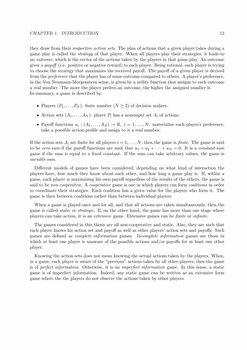
they draw from their respective action sets. The plan of actions that a given player takes during agame play is called the strategy of that player. When all players play their strategies, it leads toan outcome, which is the vector of the actions taken by the players in that game play. An outcomegives a payoff (i.e. positive or negative reward) to each player. Being rational, each player is tryingto choose the strategy that maximizes the received payoff. The payoff of a given player is derivedfrom the preference that the player has of some outcome compared to others. A player’s preference,in the Von Neumann-Morgenstern sense, is given by a utility function that assigns to each outcomea real number. The more the player prefers an outcome, the higher the assigned number is.In summary, a game is described by:
• Players (P1, . . . , PN ): finite number (N ≥ 2) of decision makers.
• Action sets (A1, . . . , AN ): player Pi has a nonempty set Ai of actions.
• Payoff functions ui : (A1, . . . , AN ) → R, i = 1, . . . , N : materialize each player’s preference,take a possible action profile and assign to it a real number.
If the action sets Ai are finite for all players i = 1, . . . , N , then the game is finite. The game is saidto be zero-sum if the payoff functions are such that u1 + u2 + · · · + uN = 0. It is a constant-sumgame if the sum is equal to a fixed constant. If the sum can take arbitrary values, the game isvariable-sum.
Different models of games have been considered, depending on what kind of interaction theplayers have, how much they know about each other, and how long a game play is. If, within agame, each player is maximizing his own payoff regardless of the results of the others, the game issaid to be non-cooperative. A cooperative game is one in which players can form coalitions in orderto coordinate their strategies. Each coalition has a given value for the players who form it. Thegame is then between coalitions rather than between individual players.
When a game is played once and for all, and that all actions are taken simultaneously, then thegame is called static or strategic. If, on the other hand, the game has more than one stage whereplayers can take action, it is an extensive game. Extensive games can be finite or infinite.
The games considered in this thesis are all non-cooperative and static. Also, they are such thateach player knows his action set and payoff as well as other players’ action sets and payoffs. Suchgames are defined as complete information games. Incomplete information games are those inwhich at least one player is unaware of the possible actions and/or payoffs for at least one otherplayer.
Knowing the action sets does not mean knowing the actual actions taken by the players. When,in a game, each player is aware of the “previous” actions taken by all other players, then the gameis of perfect information. Otherwise, it is an imperfect information game. In this sense, a staticgame is of imperfect information. Indeed, any static game can be written as an extensive formgame where the the players do not observe the actions taken by other players.

CHAPTER 1. INTRODUCTION 14
A static game can also be of incomplete information when some players are not certain about theaction sets and the payoffs of others. Harsanyi [44] has proposed a way to model and understandsuch games by introducing an initial move by “nature” that determines the“types” (action set andpayoff) for the players. This initial move is done according some prior probability. Such games arecalled Bayesian because of their inherent probabilistic nature.
Probabilistic moves also characterize models of stochastic games. Such games progress as asequence of states. In each state, players take actions and receive payoffs that depend on thecurrent state of the game, and then the game transitions into a new state with a probability basedupon the players’ actions and the current state.
Each game model considers a solution concept that determines the outcome of the game and itscorresponding strategies. Nash equilibrium (NE) is the most famous concept of game solution. Inthis thesis, we are only concerned with NE. For details about other solution concepts, we refer theinterested reader to [40] and [41].
A NE is a set of strategies of the game under which no single player is willing to unilaterallychange his strategy if the strategies of the other players are kept fix. Formally, the action profilea∗ = (a∗1, a
∗2, . . . , a
∗N ) is a Nash equilibrium if
ui(a∗) ≥ ui(ai, a∗−i), for all i = 1, . . . , N, and all ai ∈ Ai; (1.1)
where a∗−i denotes the profile of actions of all players except Pi.Whenever, for a fixed profile a−i, an action a ∈ Ai for player Pi verifies ui(a, a−i) ≥ ui(a, a∗−i) for allother a ∈ Ai, then a is said to be a best response to profile a−i for player Pi
¶. From this, we derivethe following equivalent definition for a Nash equilibrium: an action profile a∗ = (a∗1, a
∗2, . . . , a
∗N ) is
a Nash equilibrium if and only if for each player Pi, the action a∗i is a best response to the actionprofile a∗−i.
If the equilibrium strategy designates a particular action for each player, then we refer to it as purestrategy equilibrium. Pure strategy equilibria do not always exist. However, for a finite, 2-playergame an equilibrium can always be achieved by randomizing the choice of actions on the action sets(John Nash [45]-1951). Such equilibrium is called a mixed strategy equilibrium. Formally, a purestrategy is defined as a deterministic choice of action, while a mixed strategy chooses a probabilitydistribution on the set of actions.
In this thesis, because of the competitive aspects of the games we consider, pure strategy equi-librium will, most of the time, not exist. As a consequence, we are particularly interested in mixedstrategy Nash equilibria. We typically have two players: a defender and an attacker. The defenderis trying to choose an action to minimize the potential damage that an attacker could cause bytaking some attack action. The attack’s goal is to maximize the damage. In this sense, we willmost of the time be using zero-sum games. For zero-sum games, the Nash equilibrium strategiesare known to correspond to the max-min equilibria (Von Neumann-Morgenstern 1928, John Nash
¶Notice that in this definition, we do not not make the difference between action and strategy. However, thecorrect definition considers strategies (action plans) and not actions.

CHAPTER 1. INTRODUCTION 15
1951). A max-min strategy for player P is a strategy that maximizes the worst outcome that otherplayers could impose to P by their strategy choices. We use this result to compute NE, mostly inthe first two game models considered in this thesis.
Another way to find NE is by analyzing best responses. We use this tool to analyze NE in thethird game model studied in this thesis. The main result about best response is that in equilibrium,every action that is assigned a strictly positive probability by a mixed strategy for some player is abest response to the other player’s strategy.
Computing Nash equilibria is in general a difficult problem. For 2-player, finite, zero-sum games,we know that the NE strategies correspond to the max-min equilibrium strategies. Max-min strate-gies can be solved by casting the problem as a linear program [46, Chap. 11]. Linear program canbe solved by algorithms that run in polynomial time [46, Chap. 4] in the size of the problem. As aconsequence, finite, 2-player, zero-sum games can be solved in polynomial time. For general finite,2-player games, Papadimitriou [47] has shown that the problem of computing a Nash equilibriumis PPDA-complete (“Polynomial Parity Arguments on Directed graphs”). In this thesis, we willshow how to find polynomial-time algorithms for a class of quasi-zero-sum games.
1.7 Related work
As was stated earlier, there are currently many activities into applying game theoretic tools tothe security problem. The approaches used to study the communication security problem throughGame Theory can be classified in two groups (although a lot of papers combine the two). Socio-Economic approaches consider the social and economic aspects of security and have studied (amongothers), the incentives ([48],[20]) of agents involved in the security process (attackers, networkadministrators, and simple users), their behaviors ([49],[50]), and the economics of informationsecurity ([37], [51],[52]). The second approach uses Game Theory to understand the theoreticalfoundation of the security problem and to derive technical solutions ([53],[54],[55],[56],[57]).This thesis focuses on this second line of thoughts.
The book by Buttyan and Hubaux [39] considers the application of Game Theory to WirelessNetwork security problems. That of Alpcan and Basar [21] covers a wide range of security as-pects through the lenses of Game Theory. [58] is a compilation of the GameSec2010 conferenceproceedings. The surveys [34]-[35] give a broad overview of the current status of this “new” fieldof research. [34] classifies the research activities according to the game models used, while in [35],current research efforts are grouped based on the network security problems that are considered.Some of the research efforts mentioned in those surveys are discussed next.
Intrusion Detection Systems are among the subjects of network security to which Game Theoryhas been applied the most. This logically follows from the fact that traditional IDSs are based onDecision Theory and, as we have discussed earlier, for the security problem, Game Theory seems tobe more appropriate than Decision Theory. In [21], game theoretic approaches to IDS are discussedfor various game models and two chapters (9 and 10) are solely devoted to this subject. [35, Sec.

CHAPTER 1. INTRODUCTION 16
5] devoted an entire section to game theoretic approaches to IDS. Cavusoglu and Raghunathan[57] compare the use of Game Theory and Decision Theory to the detection software configurationproblem when the attackers are strategic. Their study has confirmed the conjecture that in general,the game theoretic approach is more appropriate than the decision theoretic approach.
The many game theoretic applications to IDS mentioned in [34] and [35] are mostly differentby the type of games considered in the models. In [59], Alpan and Basar study the interactionbetween a distributed IDS and an attacker and model it as a two-player, non-zero sum, one-shotgame. The model is refined in [60] in an extensive form game where a network sensor playingthe role of “nature” moves first by choosing a probability of attack (and no-attack), then theIDS and the attacker move simultaneously. In [61], a multi-stage dynamic game model is used tostudy the intrusion detection problem in a mobile ad hoc network. Zhu and Baser [62] model theconfiguration problem of policy-based IDS as a stochastic dynamic game. A stochastic game modelis also considered by Liu et al. [56] for the insider attack problem. Zonouz et al. [63] model theinteraction between a response engine and an attacker as a Stackelberg game where the engine isthe leader and the attacker the follower. A Bayesian game approach is proposed in [64] to studythe intrusion detection problem in wireless ad hoc networks.
As proofs of concept (application of Game Theory to security), we believe that all these worksare complementary to our intelligent virus game model. The intruder game treated in chapter 2of this thesis departs a bit from those models. In our model, we are not interested in detectingthe presence of an intruder; rather, we focus our attention on how much trust a receiver shouldhave in a received message that has transited via a potentially compromised relay. In that sense,our intruder game is closer to [65], where the author treats the problem of false disseminationof information in a vehicular network. Our work is also closely related to the attacks on ad hocnetwork routing protocols discussed in [39, Chap. 7].
Trust and Deception is an important subject that has received a lot of attention in the years.Kevin Mitnick‖, the infamous hacker and “social engineer” explains in his book, the Art of De-ception, how to bypass the most efficient firewalls and encryption protocols by fooling users in anetwork to gather confidential information. The book by Castelfranchi [66] treats the subject oftrust and deception in virtual societies.
Availability is one of the security requirements that requires that network resources and assetsare available to legitimate users when needed. In an availability (or denial-of-service) attack,the hacker targets a resource that the defender (might) need to perform a certain task. In thatsense, our blocking security game model can be interpreted as an availability game. The jamminggames presented in ([67]-[68]) are other examples of availability games. In [67], Zander considersthe problem of multihop packet radio networks (PRNs) in the presence of an active jammer. Thesituation is modeled as a two-player constant-sum game where both the jammer and the attacker aresubject to an average power constraint. The optimum jamming strategies as well as the best medium
‖David Kevin Mitnick was one of the most notorious cyber thieves. Over a 13 year period, he broke into thecomputer systems of more that 35 international organizations. He was on the FBI’s list of most wanted criminalsand was arrested in 1995 and sentenced to 5 years prison. Mitnick now runs “Mitnick Security Consulting”.

CHAPTER 1. INTRODUCTION 17
access policies are derived. Kashyap et al. [69] consider the jamming problem in a MIMO GaussianRayleigh fading channel scenario. The interaction between the jammer and the transmitter-receiverpair is modeled as a zero-sum game where the attacker is trying to minimize the mutual informationbetween the transmitted and received signal, while the defenders are trying to maximize it. Altmanet al. consider a similar problem where the value of the game is the signal to interference-plus-noiseratio (SINR).
The work in [55] is another denial-of-service attack game where an attacker on the Internet istrying to deface the homepage on a given server. A stochastic game approach is proposed betweenthe network administrator and the attacker where at each time step, both players choose theiractions and the game moves to a new state according to some probability that depends on thechosen actions. Through simulations, the authors have shown that the game admits multiple Nashequilibria. Since a NE gives to the defender an idea about the attacker’s best strategies, findingmore NE means having more information about the attack.
All these games (and others cited in [34] and [35]) head to the same direction as our blockingsecurity game models in the sense that resources that might be (or are) needed by the network arethe target of attacks. They consider a variety of game models and different techniques to computeNash equilibria. In that, we consider them complementary to our work. Our model is howevermore general, permitting us to cover a broad range of problem. Furthermore, we have analyticallycharacterized the set of Nash equilibria in our models.
Although not dealing with an availability issue, the work presented in [70] is particularly close tothe examples of network design we have presented in this thesis. In that paper, the authors considera non-cooperative, multi-player game on a graph, with two kinds of players, a set of attackers anda protector player, representing the viruses and the system security software, respectively. Eachattacker chooses a node of the graph to infect and the protector chooses a simple path (or edge)to protect. As in our case, the authors relate the mixed Nash equilibria of the game to graph-theoretic notions (edge cover and vertex cover) and suggest polynomial time algorithm to computeNash equilibria. Our work however departs from their paper in two ways. First, the graph examplespresented in this thesis are just applications of a general model to particular cases. Our model coversa broad range of security problems which include the one considered in their paper. Second, inour example the network is interested in choosing links, while in their paper, the network protectsnodes.
The Nash equilibria characterization provided in this thesis can be considered as an applicationof the result in [71] to the particular case of quasi zero-sum game. Although Avis et al. were notinterested in characterizing Nash equilibria (which would be very laborious for an arbitrary two-player matrix game) and did not explicitly consider the notion of blockers, all the ingredients wehave used in our NE characterization can be derived from their results. Our use of the combinatorialnotion of blocker was the key to our success in characterizing the mixed strategy Nash equilibria ofthe game. To our knowledge, such a notion was not used before in the context of computing Nashequilibria.
We derive polynomial time algorithms by relating the Nash equilibria computation problem to

CHAPTER 1. INTRODUCTION 18
the minimization of submodular functions ([72, Chap. 9],[73]). Polynomial time algorithms areknown to exist for zero-sum bimatrix games via Convex Optimization methods [74, Chap. 11].However, computing Nash equilibria for a general two-player matrix game is known to be PPAD-complete∗ [47]. In that sense, our work extends (although very modestly) the class of games thatare known to be solvable in polynomial time.
∗Polynomial Parity Arguments on Directed graphs

19
Chapter 2
Intruder Game
This chapter presents a communication scenario where not all network components are trustworthy–because some of them might be compromised. More concretely, we consider the situation where agiven network agent (node) is receiving some information via another agent (or relay) which mightbe compromised by an attacker. If the relay is compromised, the goal of the attacker is to corruptthe information in order to deceive the receiver. The receiver (defender) cannot distinguish betweena compromised relay and a normal one. Upon receiving the information, the receiver then has todecide how much to trust it.
In section 2.1, we model the interaction between the attacker and the defender as a zero-sumgame. We study a simple model where the message expected by the receiver is a binary randomvariable drawn from 0, 1 according to a known probability distribution. In this case, the attackeris just trying to figure out whether to flip a received bit of not. When the receiver gets somedata, he will decide whether to trust it or not. Indeed, the model holds for non-binary messages.However, characterizing the NE in those cases can easily become overwhelming. Software programslike GAMBIT [75] can help compute Nash equilibria in certain cases.
By analyzing the Nash equilibrium of the game, we have found that, unless the chances that therelay gets compromised are small, the receiver should never trust the received message. If thosechances are relatively small, the receiver should always trust the received message, despite the factthat the best attacker will always corrupt the message. The equilibrium strategies also suggestthat, in general, the most aggressive attackers are not always the most dangerous ones.
In section 2.3, we introduce a challenge-response mechanism. The challenge-response is a processunder which the receiver has the option to pay a certain cost and use a secure channel to verifythe message (and detect the presence of the attacker if there is any). When detected, the attackerincurs some penalty. The analysis of the NE in this case shows that, by using a challenge, thereceiver can completely deter the attacker from attacking.

CHAPTER 2. INTRUDER GAME 20
2.1 Simple Intruder Game
We consider the communication model depicted in figure 2.1.We use names in the security jargon (Alice, Trudy, Bob), to designate the agents involved inour security games. These agents can, however, be any network component capable of storing,transferring, or processing information.
p
1-p
Alice Trudy
Bob X Y Z
Figure 2.1: Intruder game model. Alice sends a message to Bob. The message might transit via anattacker: Trudy. The game is between Bob who wants to correctly detect the message and Trudywho wants to corrupt it.
Alice sends a message X to Bob through a channel. The channel is insecure in the sense thatan intruder, Trudy, might be present and is able to corrupt the message. This captures the caseswhere a malicious user is present in a communication system or that communication componentscan be compromised by malicious users.
The message X is considered to be a binary random variable (X ∈ 0, 1) drawn from the set0, 1 according to a probability distribution Pr[X = x] = π(x), x ∈ 0, 1 that is assumed to beknown to Bob and Trudy∗. We let Y designate the message that Bob receives.
Trudy is present with a probability p known to both Trudy and Bob. This can be interpretedas if Trudy has only p chance of getting the message or that a fraction equal to p of the networkcomponents is corrupted (either by a malicious user, or by being themselves malicious).
When Trudy is not present, Bob correctly receives the message sent by Alice Y = X. When Trudyis present, we model her possibly randomized strategy that modifies X into Y by the probabilitiesP (x, y) = Pr[Y = y | X = x] for x, y ∈ 0, 1. P is hence a 2× 2 stochastic matrix.
Upon receiving a message Y from the channel, Bob guesses that Alice sent the message Z. Wemodel Bob’s decision by the probabilities Q(y, z) = Pr[Z = z | Y = y] for y, z ∈ 0, 1. Let C(x, z)be the cost that Bob faces when he decides Z = z when X = x, for x, z ∈ 0, 1. For given choicesof the probabilities P and Q, the expected cost J(P,Q) = E(C(X, Z)) can be calculated as follows:
J(P, Q) =∑x,y,z
π(x)R(x, y, z)C(x, z) (2.1)
where R is the matrix given by
R(x, y, z) = [(1− p)I + pP (x, y)]Q(y, z), (2.2)∗Alice is not part of the game

CHAPTER 2. INTRUDER GAME 21
where I is the 2 × 2 identity matrix. The term (1 − p)I + pP (x, y) in this expression means thatwith probability 1 − p the message is faithfully received, and with probability p, it gets modifiedby the intruder (according to the stochastic matrix P (x, y)).
Trudy’s goal is to choose P to maximize J(P, Q) whereas Bob’s goal is to choose Q to minimizeJ(P, Q). This scenario is modeled by a Bayesian zero-sum game ([40],[41]).
2.2 Nash Equilibrium
Recall that in a two-player zero-sum game, the Nash equilibrium corresponds to the max-minequilibrium ([40, Chap.2]) and is a pair (PNE , QNE) such that
J(PNE , QNE) = maxP
minQ
J(P,Q) = minQ
maxP
J(P, Q). (2.3)
That is, neither Alice nor Bob can gain by deviating from those choices.
To analyze the Nash equilibria of the game, we assume that C(0, 0) = C(1, 1) = 0, which meansthat Bob does not incur any cost when he correctly guesses Alice’s message. Also, we assume,without loss of generality, that π(0)C(0, 1) ≤ π(1)C(1, 0). (We could interchange the roles of 0 and1 if the inequality does not hold.)
Theorem 1 The Nash equilibria, as a function of the parameter p, are shown in figure 2.2, whereP1 is a set of stochastic matrices P such that
p (π(0)P (0, 1)C(0, 1) + π(1)P (1, 0)C(1, 0)) ≥ π(0)C(0, 1). (2.4)
P2 is a set of stochastic matrices P such that the previous inequality holds and, moreover,
p (π(0)P (0, 1)C(0, 1) + π(1)P (1, 0)C(1, 0)) ≤ π(1)C(1, 0). (2.5)
The values r1 and r2 are defined by
r1 = 1− r2 =π(0)C(0, 1)
π(0)C(0, 1) + π(1)C(1, 0). (2.6)
2.2.1 Understanding the NE
The meaning of this result is as follows.When the probability p that Trudy is present is smaller than r1, Bob should always trust thereceived message (and choose Z = Y ). The corresponding strategy for Trudy is to always corruptthe message as Y = 1 − X whenever she is present. This might seem counter-intuitive (for Bob)but it is not. In fact, Bob does not know when Trudy is present or not, but he knows that Trudy

CHAPTER 2. INTRUDER GAME 22
Figure 2.2: The Nash Equilibria of the Intruder Game. The figures in the right show the regionsP1 and P2.
is absent most of the time (p small). Thus, although Trudy is always corrupting the message, therisk of trusting the channel is small for Bob (think of p ≈ 0).
When p is larger than r1, Bob should always ignore the message Y because it is “too” untrust-worthy. For this strategy to hold as NE strategy for Bob, Trudy should corrupt the message withappropriate probabilities, which corresponds to the conditions (2.4)-(2.5) on P . These conditionsare represented by the regions P1 and P2 of figure 2.2, respectively.
To understand (2.4), note that the left-hand side is Bob’s expected cost if he trusts the receivedmessage and chooses Z = Y . The right-hand side is his cost if he (ignores the message and) choosesZ = 1. Also, we will show later that for r1 ≤ p ≤ r2, choosing Z = 0 will always be suboptimal forBob, independently of Y . Thus, the condition means that Bob should chooses Z = 1.
Similarly, the right-hand side of (2.5) is Bob’s expected cost if he chooses Z = 0. That conditionimplies that Bob should not choose Z = 0 and the first condition implies that he should not chooseZ = Y . Hence, Bob’s best strategy is Z = 1 independently of the received message Y . The upperbound π(1)C(1, 0) imposes some maximum values for P (0, 1) and P (1, 0). This implies that Trudycannot be too aggressive. To see this, assume that Trudy is so aggressive that condition (2.5) isviolated. Then, consider a strategy where Bob always chooses Z = 1− Y . The corresponding costis equal to Pr[X = 0, Y = 0]C(0, 1) + Pr[X = 1, Y = 1]C(1, 0), which, by extending the terms,gives
π(0)C(0, 1) + π(1)C(1, 0)− p (π(0)P (0, 1)C(0, 1) + π(1)P (1, 0)C(1, 0)) . (2.7)
This is less than π(0)C(0, 1) if condition (2.5) is violated. Thus, Bob can obtain a better payoffby changing his strategy from Z = 1 to Z = 1 − Y . As a consequence, for Trudy to achieve thehighest possible payoff, she must limit her aggressiveness to satisfy (2.5).
2.2.2 Proof of theorem 1
To simplify notation, we let C(0, 1) = A, C(1, 0) = B, P (i, j) = 1 − P (i, i) = pi, and Q(i, j) =1−Q(i, i) = qi for i 6= j ∈ 0, 1 (which are the probabilities of flipping).

CHAPTER 2. INTRUDER GAME 23
With these new notations, the expected cost can be written as:
J(P, Q) = π(0) ((1− pp0)q0 + (1− q1)pp0) A + π(1) ((1− pp1)q1 + (1− q0)pp1) B (2.8)= q0 (π(0)A− T ) + q1 (π(1)B − T ) + T (2.9)
where identity (2.9) is obtained by rearranging the terms in the RHS of (2.8) and T is defined asT = p [π(0)p0A + π(1)p1B].
First, notice that Bob can always achieve a cost of π(0)A ≤ π(1)B by completely ignoring themessage and choosing Z = 1 (this is equivalent to q0 = 1 and q1 = 0–always flip a 0 and alwaysaccept a 1).
Now, minimizing the expression (2.9) over Q, we see that Bob’s best response to any strategy Pis to choose (q0, q1) such that q0 = q1 = 0 if T < π(0)A; q0 = 1 − q1 = 1 if π(0)A < T < π(1)B;and q0 = q1 = 1 if T > π(1)B. The corresponding costs are T , π(0)A, and π(0)A + π(1)B − Trespectively for T < π(0)A, π(0)A < T < π(1)B, and T > π(1)B. If Q is such that T = π(0)A(resp. T = π(1)B), Bob is indifferent and can choose any 0 ≤ q0 ≤ 1 (resp. 0 ≤ q1 ≤ 1). Thus, wefind that
minQ
J(P,Q) =
T, if T < π(0)Aπ(0)A, if π(0)A ≤ T ≤ π(1)Bπ(0)A + π(1)B − T, if T > π(1)B.
(2.10)
Trudy’s best strategy is obtained by maximizing minQ J(P, Q) with respect to P . For that, welet p vary between 0 and 1, and examine how the best responses are changing.
• If 0 ≤ p < r1, then for all values of (p0, p1), T < π(0)A. We have already shown that Bob’sbest response in this case is Z = Y (i.e. q0 = q1 = 0). Trudy’s best strategy is obtained bymaximizing the corresponding cost (T ). The optimal value is achieved at p0 = p1 = 1, sothat Y = 1−X. Thus, for 0 ≤ p < r1, the strategies given in the theorem are best responsesto each other. As a consequence, they form a NE.
• If r1 ≤ p ≤ r2, then for some values of (p0, p1), T is less then π(0)A and for others, T ≥π(0)A. Notice that the maximum value of T is π(1)B. If (p0, p1) is such that T ≤ π(0)A,then the corresponding cost is T ≤ π(0)A (see (2.10) second row). If, on the other handπ(0)A < T ≤ π(1)B, then the cost is π(0)A. This second strategy dominates the first, thus,the best strategy for Trudy is to choose (p0, p1) such that π(0)A < T ≤ π(1)B. Bob’s best betin this case is to choose Z = 1. Consequently, any P ∈ P1 and Z = 1 is a Nash equilibrium.
• If r2 < p ≤ 1, then, depending on the choice of (p0, p1), one can have T ≤ π(0)A, π(0)A <T ≤ π(1)B, or π(1)B < T . A similar reasoning as in the previous case shows that if (p0, p1)are chosen such that π(0)A ≤ T ≤ π(1)B, then Bob’s best response is q0 = 1 − q1 = 1.This leads to a payoff of π(0)A. If Trudy chooses (p0, p1) such that π(1)B < T , we haveseen in our discussion above (2.7), that Bob can choose a strategy (Z = 1 − Y ) to achievea payoff that is less than π(0)A. Thus, the best bet for Trudy is to make her choice satisfyπ(0)A ≤ T ≤ π(1)B. This implies that any P ∈ P2 and Z = 1 is a Nash equilibrium.

CHAPTER 2. INTRUDER GAME 24
Notice that at the boundary T = π(0)A, Bob can choose any value for q0, but q1 = 0.Similarly, when T = π(0)A, Bob can choose any value for q1, but q0 = 1. All these choicesyield to the same cost of π(0)A for Bob.
2.3 Challenging the Message
In this section we introduce a challenge-response mechanism for the receiver (Bob). The challenge-response is a process under which Bob has the additional choice of challenging the received messageby paying a fixed cost of V and getting an acknowledgement from Alice (see figure 2.3). We assumethat Trudy cannot corrupt the challenge communication. For example, in the case of a phishing
p
1-p Alice
Trudy
Bob X Y Z
Pay: V
Figure 2.3: The Intruder Game with Challenge.
email that pretends to come from a bank, this challenge can be interpreted as the recipient of theemail making the additional effort of taking the phone and calling the bank to verify the authenticityof the email. In general, the challenge can be thought of as Bob being able to use a secure sidechannel to verify the message with the source (Alice) and detect the presence of the attacker ifthere is any. When detected, the attacker incurs some penalty.
As in the previous sections, we model the problem as a Bayesian game and study the set of Nashequilibria. We consider the same setting as in the previous section with the following additionalfeatures:
1. Whenever Bob receives a message, he decides whether to challenge it or not. Challengingrequires the payment of a fixed cost of V . We let α(y) be probability that Bob challenges amessage Y = y, for y = 0, 1.
2. If he decides not to challenge the message, then Bob is back to the decision problem consideredin the previous section: should he trust the message or not? In that case, we model his strategywith the matrix Q.
3. If the challenged message turns out to be corrupted, then the intruder (Trudy) is punishedby having to pay a fine V †.
†Typically the punishment is larger than the challenge cost. We have considered these costs to be equal forsimplicity.

CHAPTER 2. INTRUDER GAME 25
4. If Bob challenges a received message and finds out that it was correct (i.e. was not changed),then he looses the challenge cost of V .
5. As before the strategies for Trudy is to decide whether to corrupt the message before relayingit. We model her strategy with the matrix P , as before.
For this game, Bob pays C(X, Z)1no challenge+V 1X = Y and challenge. Accordingly, theexpected value J(P,Q, α) of Bob’s cost is given by the following expression:
J(P,Q, α) =∑x,y,z
π(x)C(x, z)R(x, y, z)(1− α(y))
+ V∑x,y
π(x) ((1− p)I(x, y) + pP (x, y))α(y)PrX = y|Y = y. (2.11)
Bob is trying to minimize this value by his choice of αi and qi for i = 0, 1. Trudy’s objective is tochoose pi, i = 0, 1 to maximize the expected value of her reward C(X,Z)1no challenge−V 1X 6=Y and challenge. This expected reward K(P, Q, α) is as follows:
K(P, Q, α) =∑x,y,z
π(x)C(x, z)R(x, y, z)(1− α(y))
− V∑x,y
π(x) ((1− p)I(x, y) + pP (x, y))α(y)PrX 6= y|Y = y. (2.12)
To analyze the Nash equilibria, we assume, as before, that π(0)C(0, 1) ≤ π(1)C(1, 0). Fur-thermore, in this section we assume that A = C(0, 1) < B = C(1, 0). We also assume thatπ(1)Bπ(0) ≥ π(0)A
π(1) . These assumptions have a slight effect in the result presented below. More pre-cisely, changing these assumptions will slightly change the decision regions. However, the sameapproach can be carried to compute the Nash equilibrium for the other cases.
Theorem 2 Figure 2.4 shows the different decision regions for the Nash equilibrium, and Table 2shows the corresponding strategies for Bob and Trudy.
In the table , β(0) = V (π(1)B−π(0)V )pπ(0)(AB−V 2)
, β(1) = V (π(0)A−π(1)V )pπ(1)(AB−V 2)
, and γ = (1−p)π(0)Vpπ(1)B .
A proof of the theorem is provided in section 2.3.2
2.3.1 Understanding the NE
The meaning of this result is as follows.The region R0 corresponds to the case when V > max(A,B) = B. In this case the challenge costis too high, and the receiver is better off to never use it. Instead, Bob will optimally decode as ifthere were no challenge possibility. This gives the same result as in section 2.2.

CHAPTER 2. INTRUDER GAME 26
p
V
1
B
A
Region: R0
Region: R1
Region: R2
Region: R3
Region: R4
Figure 2.4: The Nash equilibria decision regions of the Intruder Game with challenge.
Region Bob Trudy
R0 As in previous section
R1α(0) = α(1) = 0 P = I
Z = Y
R2α(0) = α(1) = 0 P ∈ P3
Z = 1
R3α(0) = B/(V + B)
α(1) = 0 P (0, 1) = 1, P (1, 0) = γZ = Y
R4α(0) = B/(V + B)α(1) = A/(V + A) P (0, 1) = β(0), P (1, 0) = β(1)
Z = Y
Table 2.1: Nash equilibria strategies for the Intruder Game with challenge.
In R2 the challenge cost is high but not high enough to be totally ignored as in region R0.Here, the challenge plays the role of a threat and obliges the attacker to reduce her aggressivenesscompared to R0. Hence, the intruder has less degrees of freedom compared to the previous section:the optimal strategy set is now P3 which is P1 (resp. P2 depending on the value of p) of theprevious section with the additional requirement that π(0)V ≥ p(P (0, 1)π(0)V + P (1, 0)π(1)B).The optimal strategy for Bob is then to not use the challenge and ignore the message.
Region R1 is the set of V that satisfies V > p1−p
π(1)Bπ(0) (or (1 − p)π(0)V > pπ(1)B). Notice
that such V also satisfies V > p1−p
π(0)Aπ(1) (or (1 − p)π(1)V > pπ(0)A) because of the assumption
π(0)A ≤ π(1)B. The term (1 − p)π(0)V (resp. (1 − p)π(1)V ) is the cost of challenging when a0 (resp. 1) is sent and there is no intruder, while the term pπ(1)B (resp. pπ(0)A) represents theaverage cost of accepting a 1 while a 0 (resp. 1) was sent and the intruder is present. The inequalitiesabove tell that, for Bob, in either case, the expected cost of challenging a message is higher thanthe that of accepting it. Thus, Bob is better off to not use the challenge (α(0) = α(1) = 0) and

CHAPTER 2. INTRUDER GAME 27
to optimally decode as if there were no challenge. Since in this region p ≤ r1, the best decodingstrategy is Z = Y (always accepting the message as in the previous section) and Trudy will alwayschange the message. As was discussed in the previous case, Bob can trust the message becausemost of the time Trudy is absent and the challenge is too high to be used. The average cost for Bobis equal to p(π(0)A + π(1)B) ≤ π(0)A, which is equal to the expected reward that Trudy receives.
R3 can be described as (1− p)π(0)V < pπ(1)B and π(1)V > pπ(0)A. In this region, the risk ofchallenging a 0 ((1−p)π(0)V ) if Trudy is not present, is less than the cost of wrongly accepting a 1(pπ(1)B) if she is present and happens to flip the bit. Thus, Bob is better off challenging a receivedY = 0. However, since the intruder is present only a fraction of time, challenge should also occura fraction of time (α(0) = B
B+V ). When Bob does not challenge a received Y = 0, he will trustit (Z = Y ). With the assumption π(0)A ≤ π(1)B, the expected cost of accepting a 1 is alwaysless than the cost of not accepting it. And, since the challenge cost is relatively high compared topπ(0)A, Bob is better off to never challenge 1 and to always accept it (α(1) = 0 and Z = Y whenY = 1). The corresponding best strategy for the intruder is to always flip a 0, and to flip a 1 onlya fraction of time γ. The average cost for Bob is π(0)(pA + (1− p)V ) < π(0)A, while the expectednet attack reward received by Trudy is pπ(0)A.
In region R4 the challenge risk is small enough for Bob to challenge both messages. As aconsequence, Trudy will flip only a fraction of time (β(0), β(1)). Interestingly, in this region, theaverage cost for Bob is AB−(π(0)A+π(1)B)
AB−V 2 V < V ‡ while the average reward for Truder is equal tozero; i.e the intruder has no incentive to attack. Thus, by using the challenge (as a credible threat),Bob can deter Trudy from attacking the communication.
Compared to the previous case, we have seen that the challenge gives to the receiver the possibilityto always trust the channel (Y = Z) when V ≤ minC(0, 1), C(1, 0) without having to pay theworst case cost of π(0)A. Furthermore, with relatively cheap challenge, the receiver can deterthe intruder from attacking. This tells that with a simple challenge-response scheme, one canimplement a perfect§ communication over an insecure channel.
2.3.2 Proof of theorem 2
As in the proof of the theorem in the previous case, we simplify the notation by letting C(0, 1) =A, C(1, 0) = B, P (i, j) = 1− P (i, i) = pi, and Q(i, j) = 1−Q(i, i) = qi for i 6= j ∈ 0, 1.
By extending and arranging the terms in equation (2.11) (resp. (2.12)), we can rewrite theexpected cost (resp. reward) of the receiver (resp. attacker) as
J(P, Q, α) = T + α(0) (π(0) (1− pp0) V − π(1)pp1B) + (1− α(0))q0 (π(0)A− T )+ α(1) (π(1) (1− pp1) V − π(0)pp0A) + (1− α(1))q1 (π(1)B − T ) , (2.13)
‡Note that as p goes to zero, V also goes to zero and so does the attack cost for Bob.§This requires the channel used for the challenge to be secure itself. Also, the meaning given to perfect is that the
attacker does not have an incentive to attack.
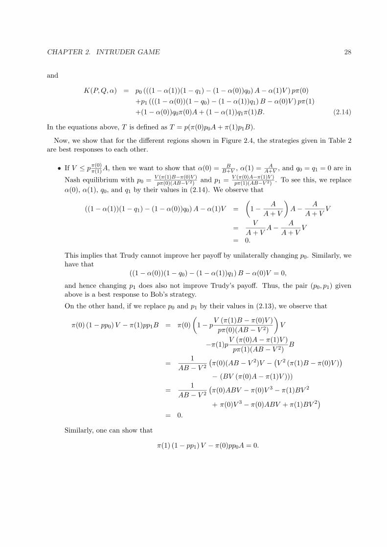
CHAPTER 2. INTRUDER GAME 28
and
K(P,Q, α) = p0 (((1− α(1))(1− q1)− (1− α(0))q0) A− α(1)V ) pπ(0)+p1 (((1− α(0))(1− q0)− (1− α(1))q1)B − α(0)V ) pπ(1)+(1− α(0))q0π(0)A + (1− α(1))q1π(1)B. (2.14)
In the equations above, T is defined as T = p(π(0)p0A + π(1)p1B).
Now, we show that for the different regions shown in Figure 2.4, the strategies given in Table 2are best responses to each other.
• If V ≤ pπ(0)π(1)A, then we want to show that α(0) = B
B+V , α(1) = AA+V , and q0 = q1 = 0 are in
Nash equilibrium with p0 = V (π(1)B−π(0)V )pπ(0)(AB−V 2)
and p1 = V (π(0)A−π(1)V )pπ(1)(AB−V 2)
. To see this, we replaceα(0), α(1), q0, and q1 by their values in (2.14). We observe that
((1− α(1))(1− q1)− (1− α(0))q0) A− α(1)V =(
1− A
A + V
)A− A
A + VV
=V
A + VA− A
A + VV
= 0.
This implies that Trudy cannot improve her payoff by unilaterally changing p0. Similarly, wehave that
((1− α(0))(1− q0)− (1− α(1))q1) B − α(0)V = 0,
and hence changing p1 does also not improve Trudy’s payoff. Thus, the pair (p0, p1) givenabove is a best response to Bob’s strategy.
On the other hand, if we replace p0 and p1 by their values in (2.13), we observe that
π(0) (1− pp0) V − π(1)pp1B = π(0)(
1− pV (π(1)B − π(0)V )pπ(0)(AB − V 2)
)V
−π(1)pV (π(0)A− π(1)V )pπ(1)(AB − V 2)
B
=1
AB − V 2
(π(0)(AB − V 2)V − (
V 2 (π(1)B − π(0)V ))
− (BV (π(0)A− π(1)V )))
=1
AB − V 2
(π(0)ABV − π(0)V 3 − π(1)BV 2
+ π(0)V 3 − π(0)ABV + π(1)BV 2)
= 0.
Similarly, one can show that
π(1) (1− pp1) V − π(0)pp0A = 0.

CHAPTER 2. INTRUDER GAME 29
Thus, Bob does not gain more by changing α(0) or α(1). To complete the proof of this case,we need to show that the choices q0 = q1 = 0 are also optimal for the the receiver. For that,it suffices to show that the term π(0)A − T is nonnegative. Indeed, since Bob is trying tominimize the expected cost (2.13), the best value for q0 is 0 whenever π(0)A− T ≥ 0. Sinceπ(1)B ≥ π(0)A, this will also mean that π(1)B − T ≥ 0. By expending the term π(0)A− T ,we get that
π(0)A− T = = π(0)A− p (π(0)p0A + π(1)p1B)
= π(0)A− p
(π(0)
V (π(1)B − π(0)V )pπ(0)(AB − V 2)
A + π(1)V (π(0)A− π(1)V )pπ(1)(AB − V 2)
B
)
=1
AB − V 2
(π(0)A(AB − V 2)−A (V (π(1)B − π(0)V ))
−B (V (π(0)A− π(1)V )))
=1
AB − V 2
(π(0)A2B − (π(0) + π(1))ABV + π(1)BV 2
−π(0)AV 2 + π(0)AV 2)
=1
AB − V 2
(π(0)A2B − (π(0) + π(1))ABV + π(1)BV 2
)
=B
AB − V 2(π(0)A(A− V )− π(1)V (A− V ))
=B(A− V )AB − V 2
(π(0)A− π(1)V ) .
Since V ≤ pπ(0)π(1)A for all p, we have that (π(0)A− π(1)V ) ≥ 0 (by considering the particular
case of p = 1). Thus, the RHS in the last equality above is greater than 0 if A−V ≥ 0, whichis what we needed.
The last step to finalize the proof in this case is to show that the value p0 and p1 given aboveare probability distributions. It is readily verifiable that they are both greater than zero. Toverify that p0 is less than one, we write
pπ(0)(AB − V 2)− V (π(1)B − π(0)V ) = B (pπ(0)A− π(1)V ) + (1− p)π(0)V 2,
which is greater than zero if V ≤ pπ(0)π(1)A. Thus, pπ(0)(AB − V 2) ≥ V (π(1)B − π(0)V ), and
as a consequence p0 ≤ 1. Similarly,
pπ(1)(AB − V 2)− V (π(0)A− π(1)V ) = A (pπ(1)B − π(0)V ) + (1− p)π(1)V 2,
which is greater than zero because of the assumption π(1)Bπ(0) ≥ π(0)A
π(1) . Thus p1 ≤ 1.
• If pπ(0)π(1)A ≤ V ≤ p
1−pπ(1)π(0)B, we need to show that α(0) = B
B+V , α(1) = 0, and q0 = q1 = 0 are
in Nash equilibrium with p0 = 1 and p1 = π(0)(1−p)Vpπ(1)B . As in the previous case, we verify that
they are best strategies to each other by showing that none of the players will gain from aunilateral deviation. Fixing (α(0), α(1)) and (q0, q1), we verify that the term that multiplies

CHAPTER 2. INTRUDER GAME 30
p0 in (2.14) is equal to pπ(0)A. Thus, p0 = 1 is a best response of the intruder. The termmultiplying p1 is equal to zero, so that the intruder does not make any gain by changing p1.On the other hand, by fixing p0 and p1, we verify that the term multiplying α(0) in (2.13) isequal to zero, implying that a change in α(0) does not improve Bob’s payoff. By using thevalues of pi, i = 0, 1, we can write
π(0)A− T = π(0)(1− p)(A− V ),
which is nonnegative for A ≥ V , justifying the choice q0 = 0 for Bob. As a consequence ofthis, we also have that π(1)B − T ≥ 0, implying that q1 = 0 is also a best response. Finallywe need to show that the term that multiply α1 in (2.13) is nonnegative (so as α(1) = 0 isoptimal). For that, we write
π(1) (1− pp1) V − π(0)pp0A =1B
(π(1)BV − π(0)
((1− p)V 2 + pAB
))
≥ 1B
(π(1)BV − π(0)AB) (2.15)
= π(1)V − π(0)A≥ 0,
where (2.15) is obtained by observing that (1− p)V 2 + pAB is at most AB. The final step ofthe proof of this case is to show that p1 ≤ 1. This follows from the assumption V ≤ p
1−pπ(1)π(0)B.
• If V ≥ p1−p
π(1)π(0)B, we first observe that α(0) = α(1) = 0 is always optimal for Bob. Indeed, in
this case, the minimum value of π(0) (1− pp0) V (i.e. π(0) (1− p) V ) is always larger that themaximum value of π(1)pp1B (i.e. π(1)pB). Thus, α(0) = 0 is optimal for Bob. Similarly, theminimum value of π(1) (1− pp1) V (i.e. π(1) (1− p) V ) is always larger that the maximumvalue of π(0)pp0A (i.e. π(1)pA), thus, the best α(1), is α(1) = 0. This means that Bob willignore the challenge, leading to the case studied in the previous section. Now since in regionR1, p is always less that r1, we have that T ≤ π(0)A ≤ π(1)B. As a consequence, the bestchoices for q0 and q1 are q0 = q1 = 0. This means that Bob will never challenge a message andwill always trust it. The best response to such strategy for Trudy is to choose p0 = p1 = 1.
• If B ≥ V ≥ A, all we need to show in that in region R2 there is a choice of p0 and p1
that satisfies T ≥ π(0)A and p(π(0)p0V + π(1)p1B) ≤ π(0)V . But, this is always the casebecause since p ≥ r1, we have that p(π(0)A + π(1)B) ≥ π(0)A. This implies that thereexist p0 and p1 such that p(π(0)p0A + π(1)p1B) ≥ π(0)A. The choices p0 = p1 = 1 isalways possible. The second condition (p(π(0)p0V + π(1)p1B)− π(0)V ≤ 0) can also alwaysbe satisfied. In fact, letting p0 and p1 such that p(π(0)p0A + π(1)p1B) = π(0)A, we getpπ(1)p1B = π(0)A−pπ(0)p0A. Replacing this value of pπ(1)p1B in the second condition andrearranging the terms,, we get −π(0)(1− pp0)(V −A) which is less than zero.
• If V ≥ B the challenge is not helpful anymore to Bob. If p ≤ r1, then V is always largerthan p
1−pπ(1)π(0)B, and we have seen that Bob should always trust and never use the challenge.

CHAPTER 2. INTRUDER GAME 31
If p > r1, then any choice of p0 and p1 possible in the case without challenge is still possiblefor Trudy (from the analysis of the case B ≥ V ≥ A), and for any such choice, Bob is betterof ignoring and not challenge the message. But, this is the strategy he already adopted inthe case without challenge.

32
Chapter 3
Intelligent Virus Game
In this chapter, we use a game theoretic approach to study the interaction between an intelligentvirus and an intrusion detection system (IDS). We consider a scenario where the virus is attemptingto infect as many machines as possible in a network protected by a simple IDS. Figure 3.1 is a sketchof the model. The normal traffic going through the network is assumed to have a known rate α.When present, the virus, while trying to infect other parts of the network, generates some additionaltraffic with a rate β that the virus designer needs to set. The IDS is trying to detect the virus asearly as possible while limiting false alarms. To detect intrusions, the IDS checks the amount oftraffic going through the network against a chosen threshold. We use a zero-sum, Bayesian gamemodel to analyze the situation.
The IDS buffers and counts the volume Xn of traffic in the interval [(n−1)T, nT ] for n = 1, 2, 3, . . .and decides that a virus is present the first time that Xn > x. T is a design parameter and isassumed to be known and x is a threshold to be chosen by the IDS. If the IDS decides that there isan infection, it then flushes the buffer to prevent the virus from infecting more machines. Bufferingintroduces some delay (T ) in the traffic. We use a Markov chain model to compute the Nashequilibrium of the game and analyze it.
We compare the average attack cost of this IDS to the one studied in [76]. The main differenceis that the one considered in this thesis quarantines the traffic while making its decision while thesecond lets the traffic through and decides later. For example, at time T , with the first IDS notraffic has not yet reached the other parts of the network, while with the second one, all the traffic
Network Virus
IDS
Normal Traffic
Figure 3.1: Intelligent virus game model.

CHAPTER 3. INTELLIGENT VIRUS GAME 33
0 1
False alarm: unit cost
Infection Cost
p 0
p 1
1-p 1
q 1-q
) p - (1 1
Figure 3.2: Markov chain model for computing the NE of the intelligent virus game with bufferingIDS.
has already gone through. Because of the different mathematical tools used to analyze the games,a quantitative comparison of the two modes of operation is not possible. As of such, we will onlyqualitatively contrast them.
3.1 The Intelligent Virus Game
In this problem, we suppose that for detection purposes, the IDS delays the traffic by bufferingit, and counts the volume Xn of traffic in the interval [(n − 1)T, nT ] for n = 1, 2, 3, . . . . T is adesign parameter that is set in advance. The IDS decides that the network is infected the first timethat Xn > x and it then flushes the buffer to prevent the virus from infecting other machines. Ifthe IDS finds that Xn < x, it transmits the Xn buffered bits of traffic. We are interested in theequilibrium of the game where the virus designer chooses β to maximize the damage that the viruscauses and the IDS chooses the threshold x to minimize it. This damage is the expected sum ofthe inspection and infection costs. In practice, such IDS requires inserting a short delay into thesystem, say 40ms, which not all network designers might like.
We consider a SIS (Susceptible-Infected-Susceptible) virus spreading model ([77],[78]). In suchmodel, a computer is first susceptible once a new virus appears. Then, eventually, the machine willget infected, and after cleaning it becomes again susceptible. A discrete version of such model isshown is figure 3.1. SIS models have been widely used in viral epidemiology [79], and computer viruspropagation [78]. Although it is not always realistic (a more realistic model would be Susceptible-Infected-Recovered SIR), SIS models offer a nice analytical framework. Interested readers arereferred to [77].
We evaluate the infection and the inspection costs of the model using a discrete time Markovchain model with time step T . The states are 0 and 1, where 0 means that the computer is notinfected and 1 that it is. Let p0 = Pr[Xn > x| No Virus] designate the probability that the IDSdeclares that the computer is infected when it is not (false alarm) and p1 = Pr[Xn > x| Virus]

CHAPTER 3. INTELLIGENT VIRUS GAME 34
x p0 p1 C(x, β)
0 ≤ x ≤ β α−xα 1 1−α
xq+1
β < x ≤ α α−xα
α+β−xα C3(x, β)
α < x ≤ α + β 0 α+β−xα γβq x−β
α(q+1)+β−x
Table 3.1: Values of the false alarm p0 and detection p1 probabilities.
the probability that the IDS declares that the computer is infected when it actually is (correctdetection). Finally, let q be the probability that the computer gets infected in one time step.
Figure 3.1 shows a diagram of the Markov chain. The transition probabilities of the Markovchain are then P (0, 1) = q and P (1, 0) = p1. Also, when the system is in state 0, it generates a falsealarm with probability p0 and this false alarm is assumed to have a unit cost. When the system isin state 1, it generates an average number of viruses equal to β(1 − p1) and we assume that eachreleased virus has an average cost equal to γ. Thus, γ measures the likelihood that a released virusis successful in infecting another computer. (More complex models are certainly plausible.)
With this model, the average cost per unit of time is
C(x, β) = p0π0 + γβ(1− p1)π1. (3.1)
where π0 (resp. π1) is the stationary probability that the system is in state 0 (resp. 1).The stationary distribution can be computed by solving the balance equations:
qπ0 = p1π1, and π0 + π1 = 1. (3.2)
Consequently,
C(x, β) =p0p1 + γβ(1− p1)q
p1 + q. (3.3)
The virus designer chooses the infection rate β to maximize this cost while the IDS computes thebest threshold to minimize it.
3.1.1 Deriving the NE
We analyze this model by assuming that the traffic Xn is uniform in [0, α] when the computer isnot infected and uniform in [β, α + β] when the computer is infected (i.e., the virus is introducingadditional traffic of constant rate β).
With this uniform assumptions, the probabilities p0 and p1 as functions of x and β are given inTable 3.1. Since an infection rate β > α will always result to 100% detection, we assume that β isless than α. The table also shows the corresponding values of the average cost C(x, β).
The value C3(x, β) in the table is equal to
C3(x, β) =α + β
(1− γβq +
(x2 + (αγβq − 2α− β)
))
α(q + 1) + β − x. (3.4)

CHAPTER 3. INTELLIGENT VIRUS GAME 35
q γ β x
0.01 0.02 150 9800.01 0.05 220 9000.01 0.10 250 7500.10 0.02 250 5800.10 0.05 150 3100.10 0.10 90 180
Table 3.2: Nash equilibrium (β, x) as a function of the parameters (q, γ).
Since the game is zero-sum, the Nash equilibrium strategies correspond to the max-min strategies.Hence, to find the NE, we first minimize C(x, β) over x in each of the intervals given above; foreach region this gives a function that only depends on β. We then maximize over β in each region,and take the maximum value across the regions. Since the calculation is very involved, we use asmall matlab script to compute the NE. The Nash equilibrium depends on the values of q, α, andγ. Table 3.2 shows some representative values when α = 1000.
3.1.2 Qualitative Comparison
In this section, we analyze how the attack cost depends on the strategy (propagation rate) of thevirus. In Figure 3.3(a) the attack cost of the IDS is shown as a function of the rate of propagationchosen by the virus. For each value of the infection rate (shown in the horizontal axis), we havecomputed the best response of the IDS which correspond to the optimal threshold for that rate.Then, we compute the cost as in (3.3) where x corresponds to the best response to β.
As can be seen in the figure, the cost of attack is small when the infection rate is small. Thistells that a less aggressive virus will cause less damage to the system. The figure also shows a smallcost of attack for high values of the infection rate. This means that a very aggressive virus willalso cause small damage to the system. In fact, since the IDS buffers the traffic while making adecision, and flushes the buffer if it detects a virus, an aggressive attack will very likely be detectedat the IDS level and will not make it into the system.
These two observations show that an intelligent virus will neither be too slow, nor too aggressive.Instead, it will choose an infection rate that balances between the potential reward of an aggressiveattack and the risk of being quickly detected. This tradeoff is given by the Nash equilibrium attackrate. It is equal to the rate that maximizes the minimum attack cost that the IDS can impose.
For comparison purposes, we have plotted in 3.3(b), the average cost of an IDS based on themodel in [76] as a function of the propagation rate of the virus. The model uses a sequentialprobability ratio test to compute the best threshold for a given infection cost and cost of falsealarm (which in [76] are the false alarm and missed detection probabilities). In our simulation, wehave assumed that the false alarm cost is fixed and the infection cost is a linear function of theinfection rate and of the time to detection. Notice that in the model, the virus is assumed to be
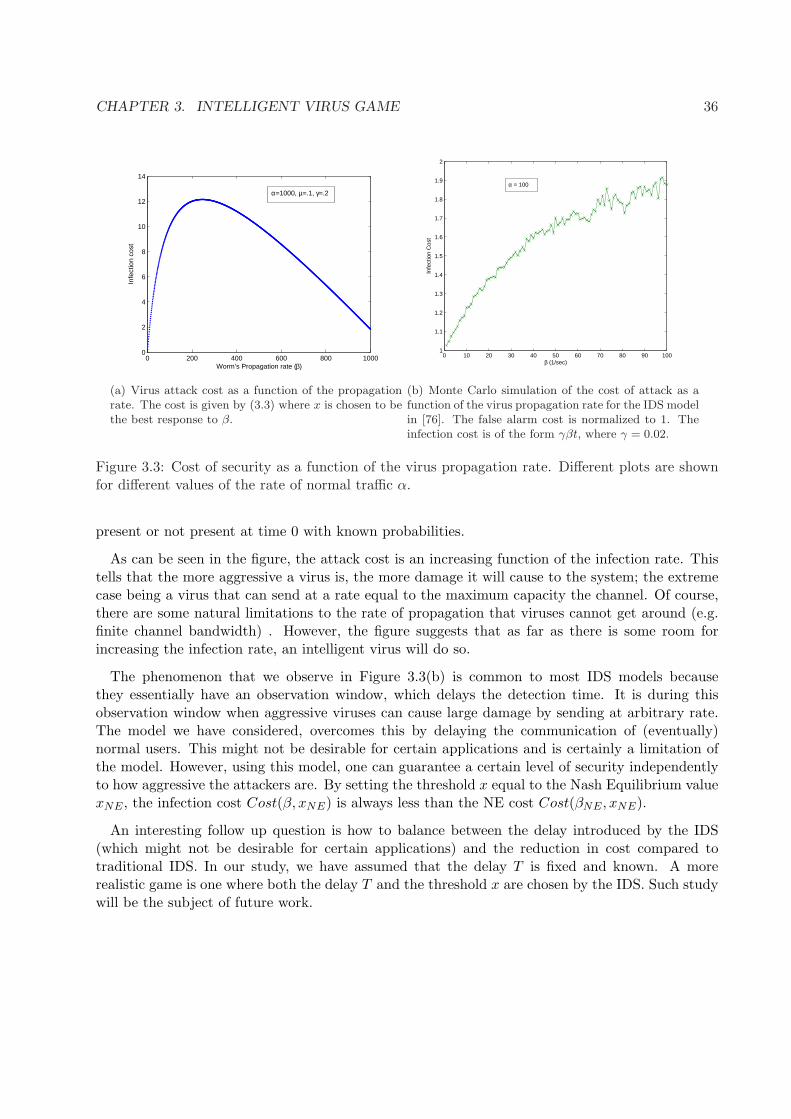
CHAPTER 3. INTELLIGENT VIRUS GAME 36
0 200 400 600 800 10000
2
4
6
8
10
12
14
Worm’s Propagation rate (β)
Infe
ctio
n co
st
α=1000, µ=.1, γ=.2
(a) Virus attack cost as a function of the propagationrate. The cost is given by (3.3) where x is chosen to bethe best response to β.
0 10 20 30 40 50 60 70 80 90 1001
1.1
1.2
1.3
1.4
1.5
1.6
1.7
1.8
1.9
2
β (1/sec)
Infe
ctio
n C
ost
α = 100
(b) Monte Carlo simulation of the cost of attack as afunction of the virus propagation rate for the IDS modelin [76]. The false alarm cost is normalized to 1. Theinfection cost is of the form γβt, where γ = 0.02.
Figure 3.3: Cost of security as a function of the virus propagation rate. Different plots are shownfor different values of the rate of normal traffic α.
present or not present at time 0 with known probabilities.
As can be seen in the figure, the attack cost is an increasing function of the infection rate. Thistells that the more aggressive a virus is, the more damage it will cause to the system; the extremecase being a virus that can send at a rate equal to the maximum capacity the channel. Of course,there are some natural limitations to the rate of propagation that viruses cannot get around (e.g.finite channel bandwidth) . However, the figure suggests that as far as there is some room forincreasing the infection rate, an intelligent virus will do so.
The phenomenon that we observe in Figure 3.3(b) is common to most IDS models becausethey essentially have an observation window, which delays the detection time. It is during thisobservation window when aggressive viruses can cause large damage by sending at arbitrary rate.The model we have considered, overcomes this by delaying the communication of (eventually)normal users. This might not be desirable for certain applications and is certainly a limitation ofthe model. However, using this model, one can guarantee a certain level of security independentlyto how aggressive the attackers are. By setting the threshold x equal to the Nash Equilibrium valuexNE , the infection cost Cost(β, xNE) is always less than the NE cost Cost(βNE , xNE).
An interesting follow up question is how to balance between the delay introduced by the IDS(which might not be desirable for certain applications) and the reduction in cost compared totraditional IDS. In our study, we have assumed that the delay T is fixed and known. A morerealistic game is one where both the delay T and the threshold x are chosen by the IDS. Such studywill be the subject of future work.

37
Chapter 4
Blocking Games
In this chapter, we consider availability (or denial of service) attacks where resources that are (ormight be) needed by a defender are the target of a cognitive attacker. More precisely, we considerthat there is a finite set S and two collections T and E of subsets of S. The defender selects asubset T ∈ T to perform a mission critical task. Each subset T ∈ T needs some set of resourceseT1 , eT2 , . . . , eTp ∈ E in order to fulfill the task. To disrupt the mission, an attacker targets oneresource e ∈ E to attack. For example, T could be the collection of spanning trees of a graphand the collection of resources E could be the edges of the graph (as we will see in our applicationexamples).
When attacked, the cost (loss) to the defender is λT,e, which models the damage caused by theattacker whenever subset T ∈ T and resource e ∈ E are selected.The reward to the attacker is λT,e − µ(e), where µ(e) is the cost of attacking the resource e ∈ E .The attacker also has the option to not launch an attack. The goal of the defender is to minimizehis loss, and the attacker is trying to maximize her net gain.
We model this situation as a “quasi” zero-sum game and consider mixed strategy Nash equilib-ria, where the defender chooses a distribution on the collection of subsets T ; and the attacker adistribution on the collection of resources E . The details of the model are discussed in section 4.2.The results of the game are discussed as a theorem in section 4.3. A proof of the theorem is pre-sented in section 4.5. Examples of applications of the model and results are discussed in section4.4.
A certain number of observations are made from the analysis of the Nash equilibria.First, there exists at least one set E ⊆ E of resources that is more vulnerable than the others – inthe sense that it gives a higher expected net reward to the attacker. Such subsets of resources arecalled critical. We use the maximum achievable reward as the vulnerability metric for the defender’stask. If the vulnerability is negative, the attacker will not launch an attack; and if it is positive,the attacker will always target critical subsets of resources. The defender will select subsets that
CHAPTER 4. BLOCKING GAMES 38
“minimally”∗ intersect the targeted critical subsets.
Second, if the defender’s loss function can be written as a submodular function, then there exists apolynomial time algorithm to compute a critical subset of resources (and hence a Nash equilibrium)for the game. We derive this algorithm by relating the computation of the vulnerability of the taskto the minimization of a submodular function. We then use the existing polynomial algorithmsfor submodular function minimization. The derivation of the algorithm is shown in section 4.6.It requires the notions of Matroid, Polymatroid, and submodular function minimization which wewill briefly discuss in the same section.
The model is applied to two examples that are discussed in section 4.4.Our first example considers a scenario where a network manager is choosing a spanning tree on thegraph of a network to connect all nodes. An attacker is trying to cut the tree by attacking one linkof the graph. One of our findings is that, in this scenario the minimum cutsets of the graph arenot the most critical subsets of links.
The second example deals with a supply-demand network where a network manager is choosing afeasible flow to transport the maximum amount of goods from a set of sources to a set of destinations,and an attacker is trying to minimize this by attacking an arc of the network. In this case, we findthat critical subsets are cutsets that maximize the minimum fraction of goods carried per link ofthe cutset. In most cases, these correspond to minimum cutsets of the graph.
Although in this thesis we focus our attention to examples on network topology, there is a broadrange of applications that fit into the framework of this model.
For general games of this model, we determine the structure of a particular set of Nash equilibria.When the game is zero-sum, we characterize the set of all Nash equilibria. Section 4.5 shows thedetails of the proof. To compute the Nash equilibria, we make use of the combinatorial tools ofblocking pair of matrices. Since these notions are central to our analysis, we start by reviewingthem in section 4.1.
Notational Conventions:In this chapter, we make the following notational conventions.We use the prime sign (’) for transpose of matrices and vectors. The column vector of ones of length|T | = N will be denoted by 1T , and 1E denotes the column vector of ones of length |E| = m. Allvectors are denoted by bold lowercase letters and are assumed to be column vectors. Matrices willbe denoted (mostly and not exclusively) by uppercase Greek letters Λ, Ω. The indicator functionwill be denoted 1cond. It is equal to 1 if “cond” is satisfied and is equal to 0 otherwise. We willuse α to designate the mixed strategy of the defender, and for the attacker, we use β. Ay otherprobability distribution will be denoted by γ.
∗This notion of minimality depends on the cost functions of the games and will become more clear once we definethose cost functions.

CHAPTER 4. BLOCKING GAMES 39
Figure 4.1: Example of polyhedron PΛ defined by a nonnegative proper matrix Λ and its corre-sponding blocker bl(PΛ). The extreme points of the blocker define the nonnegative proper matrixΩ.
4.1 Blocking Pair of Matrices
The discussion in this section is mostly based on [80, pp. 99-101] and [81].Let Λ be a N ×m nonnegative matrix with non-zero rows. The polyhedron PΛ associated with Λ isdefined as the vector sum of the convex hull of its rows (λ1, . . . ,λN ) and the nonnegative orthant:
PΛ = conv.hull (λ1, . . . , λN ) + Rm+ . (4.1)
A row λi of Λ is said to be inessential if it dominates a convex combination of other rows of Λ,otherwise we say that λi is essential. If all the rows of Λ are essential, we say that Λ is proper.The set of essential rows corresponds to the set of extreme points of the polyhedron PΛ. Sinceinessential rows are not relevant for the definition of PΛ we will drop them and assume that Λ isproper.
The example in Figure 4.1 shows the associated polyhedron PΛ to the nonnegative matrix Λgiven below:
Λ =
1/3 32/3 22 14 1/2
, Ω =
0 21/6 2/33/10 2/52/3 10/364 0
(4.2)
Given Λ and its associated polyhedron, we define the blocker of the polyhedron PΛ as follow.
Definition 1 The blocker bl(PΛ) of PΛ is the polyhedron given as:
bl(PΛ) =y ∈ Rm
+ : y′x ≥ 1, ∀ x ∈ PΛ
, (4.3)
CHAPTER 4. BLOCKING GAMES 40
where y′x is the inner product of y and x. Recall that in this thesis we use the prime sign (’) forvector and matrix transpose.
We are interested in characterizing the polyhedron PΛ and its blocker bl(PΛ). For that, we use thefollowing theorem by Fulkerson [81]. It is based on the fact that there is a one-to-one correspondencebetween the essential rows of Λ and the extreme points of PΛ.
Theorem 3 (Fulkerson, 1971) Let the N -by-m matrix Λ be proper with rows λ1, . . . , λN , andlet the polyhedron PΛ be defined as in (4.1). Let ω1, . . . , ωK be the extreme points of bl(PΛ), andlet Ω be the matrix having those points as rows. Then,
1. The blocker bl(PΛ) of PΛ is given by bl(PΛ) =x ∈ Rm
+ : Λx ≥ 1T.
2. Ω is proper, and the polyhedron PΛ can be described as PΛ =x ∈ Rm
+ : Ωx ≥ 1K
.
3. The blocker of the blocker bl(PΛ) verifies bl(bl(PΛ)) = PΛ.
Λ and Ω are said to form a blocking pair of matrices.
Equations (4.2) show a blocking pair of matrices Λ and Ω, and the corresponding polyhedra areshown in Figure 4.1.
Blocking pairs of matrices play an important role in the combinatorial problem of maximumpacking (see Fulkerson[81]). In this thesis, we use the theory of blocking pairs to provide an easyargument for the existence of a probability distribution that satisfies a certain number of constraints.For instance, consider the following linear program:
Maximize 1′T x
subject to Λ′x ≤ w, and x ≥ 0, (4.4)
where the constraints Λ form a nonnegative matrix, and w is a given nonnegative vector.We are interested to knowing whether the value of the program is greater than 1 or not. If thisis the case, one can easily derive a probability distribution by normalizing a feasible solution ofthe program. Indeed, since the normalizing factor is greater than 1, the constraints will still besatisfied. The following lemma gives an answer to our question.
Lemma 1 The value of the LP in (4.4) is greater than 1 if and only if w belongs to the polyhedronPΛ defined by Λ.
Proof: The proof of the lemma is as follow.First, notice that strong duality holds for this LP. In fact, Slater’s condition [82] is satisfied for anynonnegative and nonzero w. The dual of the LP is given as:
Minimize w′ysubject to Λy ≥ 1T , and y ≥ 0. (4.5)

CHAPTER 4. BLOCKING GAMES 41
The constraints of the dual program (4.5) define the blocker bl(PΛ) =y ∈ Rm
+ : Λy ≥ 1T
of thepolyhedron PΛ. Now, if w belongs to PΛ, then for all y ∈ bl(PΛ), we have that w′y ≥ 1.
Conversely, if w′y ≥ 1 for all y ∈ bl(PΛ), then w must be in the blocker of bl(PΛ), which byFulkerson’s theorem 3, is PΛ. This implies that the value of the dual program is greater than 1.Combined with the strong duality property, we get that the value of the primal program is at least1.
4.2 Game Model
This section presents the blocking game model and introduces some notations that we will need tocharacterize the Nash equilibria of the game.
We consider that there is a nonempty, finite set S and two nonempty collections T = T1, . . . , TNand E = e1, . . . , em of nonempty subsets of S. We call E the collection of resources. The defenderselects a subset T ∈ T to perform a mission critical task. Each subset T ∈ T needs some setof resources eT1 , eT2 , . . . , eTp ∈ E in order to fulfill the task. To disrupt the mission, an attackertargets one resource e ∈ E to attack. Each resource e ∈ E has a cost of attack µ(e) that is theamount of effort that the attacker needs to spend to successfully launch the attack. The attackeralso has the option of not attacking (“No Attack”); which we materialize by the choice of e∅. Thischoice results to zero loss for the defender and zero reward for the attacker.
Whenever the defender chooses subset T and resource e is attacked, he loses some value λT,e.This loss goes to the attacker. It is conceivable that λT,e = 0 if subset T does not need resource e.Hence, when the pair (T, e) is selected, the defender’s loss is λT,e and the attacker’s net reward isequal to λT,e − µ(e).
This scenario can be modeled as a two-player matrix game where the players (the defender andthe attacker) choose their pure strategies in the nonempty and finite sets T and E∪e∅, respectively(with |E| = m and |T | = N).The defender and attacker’s respective payoff matrices are given by
Λ = [Λ|0], and Π = [Π|0], (4.6)
where Λ and Π are N -by-m matrices; (Λ, [Λ]T,e = λT,e) is a nonnegative matrix with no zero rows†,
†A row with all zeros would lead to a trivial game because it means that there exists a subset T ∈ T that willalways result to zero loss. The defender would then always select such strategy and the game ends.

CHAPTER 4. BLOCKING GAMES 42
and such that there is no column of Λ that dominates all other columns‡. Π is given by,
Π = Λ−
µ(1) µ(2) . . . µ(m)µ(1) µ(2) . . . µ(m)
......
. . ....
µ(1) µ(2) . . . µ(m)
, (4.7)
The “last” all-zero column in the definition of Λ and Γ captures the zero-loss for the defender(λT (e∅) = 0) and zero-reward for the attacker (µ(e∅) = 0) when this latter chooses the “NoAttack” strategy (e∅). For notational simplicity, we will only mention Λ and Γ.
We consider mixed strategies of this game where the defender chooses a distribution (αT , T ∈ T )on T and the attacker chooses a distribution (β(e), e ∈ E ∪ e∅) on E ∪ e∅. The goal of thedefender is to minimize the expected loss
L(α,β) = α′Λ[β; β(e∅)] =∑
T∈TαT
(∑
e∈Eβ(e)λT,e
), (4.8)
while the attacker is trying to maximize the expected reward
R(α, β) = α′Π[β; β(e∅)] =∑
e∈Eβ(e)
(∑
T∈TαT λT,e − µ(e)
). (4.9)
In our notation, [β;β(e∅)] is the column vector obtained by appending the additional row (entry)β(e∅) to the column vector β.
Let PΛ be the polyhedron associated with Λ given in (4.6), and let bl(PΛ) denote its blocker.From the discussion in the previous section and from Fulkerson’s theorem, the blocker bl(PΛ) ⊆ Rm
+
is the polyhedron associated with the nonnegative matrix Ω whose rows are the vertices of bl(PΛ).It is also known that bl(PΛ) is the vector sum of the convex hull of rows of Ω with the positiveorthant Rm
+ , and that its blocking polyhedron is PΛ (see [81] and [80, pp. 99-101]). Also, Theorem3 gives that
PΛ =x ∈ Rm
+ , s.t. Ωx ≥ 1T
(4.10)
Now, for ω row of Ω§, which we denote as ω ∈ Ω, we write ω = (ω(e), e ∈ E), and let ω(E) :=∑e∈E ω(e). Note that ω(e) ≥ 0 for all e ∈ E and ω(E) > 0¶; so that (ω(e)
ω(E) , e ∈ E) is a probabilitydistribution on E . We call it the probability distribution induced by ω.
‡This would also lead to a trivial game if the attack cost is not too high. In fact, it means that there is a resourcethat will always give higher attack gain, independently of the subset chosen by the defender. The attacker wouldalways target such a resource.
§Notice that this is an abuse of language because ω is a column vector.¶This is because the blocker bl(PΛ) is not empty (Λ is not a one-rowed zero matrix), and does not contain the
all-zero vector (the origin) (this could not give an inner product with rows of Λ that is greater than 1).

CHAPTER 4. BLOCKING GAMES 43
Also define, for each ω ∈ Ω, the quantities
λ(ω) := minT∈T
(∑
e∈E
ω(e)ω(E)
λT (e)
); (4.11)
andθ(ω) := λ(ω)−
∑
e∈E
ω(e)ω(E)
µ(e). (4.12)
λ(ω) is the minimum loss seen by the defender if the attacker were to choose a target according tothe distribution (ω(e)
ω(E) , e ∈ E) induced by ω.The expression of θ(ω) is composed with two terms. If the attacker were to choose a resource toattack according to the distribution ω = (ω(e)
ω(E) , e ∈ E), then the first term would have been theloss seen by the defender, which, as we have assumed, goes to the attacker. The second term is theaverage cost of attack corresponding to the distribution induced by ω. Hence, θ(ω) can be seen asthe expected attack reward associated ω.
We call the vertex ω of the blocking polyhedron a critical vertex if
θ(ω) = maxω∈Ω
θ(ω) . (4.13)
A critical vertex is one whose induced probability distribution gives a maximum rewards to theattacker (considering the defender’s response).We define θ := maxω∈Ω θ(ω) to be the maximum achievable value in the preceding expression, andwe let Ωmax denote the matrix having as rows the critical vertices of bl(PΛ).We use θ as the vulnerability for the defender’s task.
4.3 Nash Equilibrium Theorem
This section presents the main results of the two-player matrix game defined in section 4.2. Weclaim that:
Theorem 4 For the game defined above, the following always hold.
1. If θ ≤ 0, then “No Attack” (i.e. β(e∅) = 1) is always an optimal strategy for the attacker. Inthis case, the equilibrium strategy (αT , T ∈ T ) for the defender is such that
λα(e) :=∑
T∈TαT λT (e) ≤ µ(e), ∀e ∈ E . (4.14)
The corresponding payoff is 0 for both players.
CHAPTER 4. BLOCKING GAMES 44
2. If θ ≥ 0, then for every probability distribution (γω, ω ∈ Ωmax), the attacker’s strategy(β(e), e ∈ E) defined by
β(e) =∑
ω∈Ωmax
γωω(e)ω(E)
(4.15)
is in Nash equilibrium with any strategy (αT , T ∈ T ) of the defender that satisfies the followingproperties:
λα(e)− µ(e) = θ for all e ∈ E such that β(e) > 0.λα(e)− µ(e) ≤ θ for all e ∈ E .
(4.16)
Further, there exists at least one such strategy α.
The corresponding payoffs are θ for the attacker, and r(γ) for the defender, where
r(γ) :=∑
ω∈Ωmax
γωλ(ω). (4.17)
3. If µ = 0, then every Nash equilibrium pair of strategies for the game is of this type.
Note: θ = 0 is a particular case where both cases (1) and (2) can occur. In all cases, themaximum achievable attack reward is equal to 0. There exist equilibria where the attacker decidesto not attack. In those cases, the defender has to choose α according to (4.14). There mightalso exist equilibria where the attack launches an attack but gets a expected reward of 0. In suchequilibrium, α has to satisfy (4.16).In our experiments we did not find any equilibrium where the attacker would mix between e∅ andsome resources in E .
4.4 Examples
In this section, we illustrate the game model and the NE theorem using two examples.The first example considers a network given as a connected undirected graph. The aim is to studythe strategic interaction between a network manager whose goal is to choose a spanning tree of thenetwork as communication infrastructure, and an attacker who tries to disrupt the communicationtree by attacking one link in the network. In the second example, we analyze games on a supply-demand network where a defender selects a feasible flow to carry a maximum amount of goodsfrom a set of sources to a set of destinations. An attacker is trying to disrupt the transport byattacking one arc of the network. We will focus our study on networks with infinite capacity onarcs. Capacitated networks can also be studied by using the same tools as un-capacitated networks.We leave this study for future work.
4.4.1 The spanning tree – link game
The network topology is given by a connected undirected graph G = (V, E) with |E| = m links and|V| = n nodes. The collection of subsets T is the set of spanning trees; we let N = |T |.
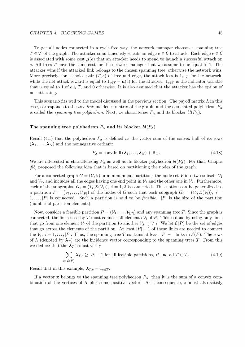
CHAPTER 4. BLOCKING GAMES 45
To get all nodes connected in a cycle-free way, the network manager chooses a spanning treeT ∈ T of the graph. The attacker simultaneously selects an edge e ∈ E to attack. Each edge e ∈ Eis associated with some cost µ(e) that an attacker needs to spend to launch a successful attack one. All trees T have the same cost for the network manager that we assume to be equal to 1. Theattacker wins if the attacked link belongs to the chosen spanning tree, otherwise the network wins.More precisely, for a choice pair (T, e) of tree and edge, the attack loss is 1e∈T for the network,while the net attack reward is equal to 1e∈T − µ(e) for the attacker. 1e∈T is the indicator variablethat is equal to 1 of e ∈ T , and 0 otherwise. It is also assumed that the attacker has the option ofnot attacking.
This scenario fits well to the model discussed in the previous section. The payoff matrix Λ in thiscase, corresponds to the tree-link incidence matrix of the graph, and the associated polyhedron PΛ
is called the spanning tree polyhedron. Next, we characterize PΛ and its blocker bl(PΛ).
The spanning tree polyhedron PΛ and its blocker bl(PΛ)
Recall (4.1) that the polyhedron PΛ is defined as the vector sum of the convex hull of its rows(λ1, . . . ,λN ) and the nonnegative orthant:
PΛ = conv.hull (λ1, . . . , λN ) + Rm+ . (4.18)
We are interested in characterizing PΛ as well as its blocker polyhedron bl(PΛ). For that, Chopra[83] proposed the following idea that is based on partitioning the nodes of the graph.
For a connected graph G = (V, E), a minimum cut partitions the node set V into two subsets V1
and V2, and includes all the edges having one end point in V1 and the other one in V2. Furthermore,each of the subgraphs, Gi = (Vi, E(Vi)), i = 1, 2 is connected. This notion can be generalized toa partition P = (V1, . . . ,V|P |) of the nodes of G such that each subgraph Gi = (Vi, E(Vi)), i =1, . . . , |P | is connected. Such a partition is said to be feasible. |P | is the size of the partition(number of partition elements).
Now, consider a feasible partition P = (V1, . . . ,V|P |) and any spanning tree T . Since the graph isconnected, the links used by T must connect all elements Vi of P . This is done by using only linksthat go from one element Vi of the partition to another Vj , j 6= i. We let E(P ) be the set of edgesthat go across the elements of the partition. At least |P | − 1 of those links are needed to connectthe Vi, i = 1, . . . , |P |. Thus, the spanning tree T contains at least |P | − 1 links in E(P ). The rowsof Λ (denoted by λT ) are the incidence vector corresponding to the spanning trees T . From thiswe deduce that the λT ’s must verify
∑
e∈E(P )
λT,e ≥ |P | − 1 for all feasible partitions, P and all T ∈ T . (4.19)
Recall that in this example, λT,e = 1e∈T .
If a vector x belongs to the spanning tree polyhedron PΛ, then it is the sum of a convex com-bination of the vertices of Λ plus some positive vector. As a consequence, x must also satisfy

CHAPTER 4. BLOCKING GAMES 46
∑e∈E(P ) x(e) ≥ |P | − 1. Using this idea, we give the following characterization (by Chopra [83]) of
the spanning tree polyhedron.
Proposition 1 The spanning tree polyhedron of the graph G corresponds to the set
PΛ =
x ∈ Rm
+ |∑
e∈E(P )
x(e) ≥ |P | − 1, ∀ P feasible partitions
, (4.20)
where E(P ) denotes the set of edges that go between vertices in distinct elements of the partition P .
We have already argued that any vector in the spanning tree polyhedron belongs to the set definedin the RHS of the equation above. To see the inverse, assume that x verifies the characterizationin the RHS of (4.20) and assume that x /∈ PΛ. This latter assumption implies that x is dominatedby any linear combination of the λT ’s, i.e.
x <∑
T∈TγT λT , (4.21)
for any (γT , T ∈ T ) such that∑
T∈T γT = 1.For any feasible partition P , there exists a spanning tree TP that contains no more than |P | − 1edges of E(P ). For such TP ,
∑e∈E(P ) λT,e = |P | − 1. Now, let (γT , T ∈ T ) be such that γTP
= 1,then (4.21) implies that
∑
e∈E(P )
x(e) <∑
e∈E(P )
∑
T∈TγT λT,e =
∑
e∈E(P )
λT,e =∑
e∈E(P )
1e∈T = |P | − 1. (4.22)
This contradicts the hypothesis that x satisfies the characterization in the RHS of (4.20). As aconsequence, x ∈ PΛ, which completes the argument.
Next, we need to characterize the blocker bl(PΛ) of the spanning tree polyhedron. Recall thatbl(PΛ) is defined as:
bl(PΛ) =y ∈ Rm
+ : y′x ≥ 1, ∀ x ∈ PΛ
. (4.23)
This is the set of nonnegative vectors y that have an inner product greater to 1 with any x ∈ PΛ.Since any x ∈ PΛ dominates a convex combination of the vertices of PΛ, we can focus on innerproducts y′x, for x vertex of the spanning tree polyhedron. We know that those vertices correspondto the rows of Λ which are the incidence vector of the spanning trees (λT ). Hence, we are lookingfor nonnegative vectors y that have an inner product equal to at least 1 with any incidence vectorλT .
We start by constructing, for any given feasible partition P = (V1, . . . ,V|P |), the vector ωP thatsatisfies (ωP )′ λT ≥ 1 for all λT . The construction goes as follows. For any feasible partition P ,form ωP whose entries correspond to the edges of the graph. Set entry ωP (e) equal to 1
|P |−1 if edgee ∈ E goes from one element Vi of the partition to another Vj (i.e. if e ∈ E(P )). Otherwise, setωP (e) = 0.

CHAPTER 4. BLOCKING GAMES 47
The claim is that the inner product (ωP )′ λT ≥ 1, for any λT . This is the case because anyspanning tree contains at least |P | − 1 edges in E(P ). The inner product is equal to 1 if thespanning tree contains exactly |P | − 1 edges in E(P ).
From this and Fulkerson’s theorem (Theorem 3), we deduce that the vectors ωP belongs to theblocker bl(PΛ) of the spanning tree polyhedron. Indeed, they have an inner product equal to atleast 1 with any x ∈ PΛ because of the fact that such x dominates a convex combination of theλT ’s.
Also, for a feasible partition P , the essential‖ vectors of the construction above are minimalin the sense that any vector y that is strictly dominated by ωP (essential) will have an innerproduct y′λT strictly less than 1 with some λT (for instance the spanning tree that crosses E(P )in exactly |P | − 1 edges). Thus, the (essential) vectors ωP must be vertices of the blocker bl(PΛ)of the spanning tree polyhedron. To show that they completely characterize bl(PΛ), we define thefollowing polyhedron (corresponding to the sum of the convex hall of those vectors plus any positivevector),
PΩ = conv.hull (ω1, . . . ,ωK) + Rm+ . (4.24)
K here is the number of feasible partitions.
Since any vector ωP has an inner product equal to at least 1 with any x ∈ PΛ, any vector y ∈ PΩ
verifies y′x ≥ 1 for any x ∈ PΛ. Thus, PΩ ⊆ bl(PΛ). Now we need to show that bl(PΛ) ⊆ PΩ. Forthat, assume that y ∈ bl(PΛ). If y /∈ PΩ, then y is dominated by any linear combination of theessential vectors ωP , i.e.:
y <∑
P
γP ωP , (4.25)
for any probability distribution γP on the set of feasible partitions P for which ωP is essential.We also know that for any feasible partition Po, there exists a spanning tree To such that
∑e∈E(Po) λTo =
|Po| − 1.
Now, let the distribution γ be such that γPo = 1 Then, (4.25) implies that
y′λTo <(ω′Po
λTo
)=
∑
e∈EωPo(e)λTo,e (4.26)
=∑
e∈E(Po)
1|Po| − 1
1e∈To (4.27)
=1
|Po| − 1
∑
e∈E(Po)
1e∈To (4.28)
=1
|Po| − 1(|Po| − 1) (4.29)
= 1 (4.30)
‖We need the vectors to be essential because a priori, a feasible partition P can yield to a ωP that is a convexcombination of the others.

CHAPTER 4. BLOCKING GAMES 48
Not feasible Not feasible Feasible Feasible
Figure 4.2: Examples of feasible and not feasible subsets of links. The chosen subset is shown indashed line. The two subsets in the left are not feasible, the two subsets in the right are feasible.
This contradicts the hypothesis that y ∈ bl(PΛ). Thus, y ∈ PΩ and as a consequence bl(PΛ) ⊆ PΩ∗∗.
This gives a characterization of bl(PΛ) by its set of vertices which are the essential vectors ofthe family defined as follow: for any feasible partition P = (V1, . . . ,V|P |), form ωP whose entriescorrespond to the edges of the graph. Set entry ωP (e) equal to 1
|P |−1 if edge e ∈ E goes from oneelement Vi of the partition to another Vj (i.e. if e ∈ E(P )). Otherwise, set ωP (e) = 0. Moreprecisely, for feasible partition P and e ∈ E ,
ωP (e) =1e∈E(P )
|P | − 1. (4.31)
From feasible partitions to feasible subsets of edges
Before applying the theory and results of the previous section to the spanning tree-link gameexample, let’s give one more result that will enable us to switch the discussion about partition toa discussion on edges of the graph.
First, observe that every feasible partition P uniquely defines the set E(P ) of edges that go acrossthe elements of P . Also, each such edge has its two ends in two different connected componentsof the graph GE(P ) obtained by removing from G, the edges in E(P ). This means that adding anyedge e ∈ E(P ) to GE(P ) will decrease the number of its connected components by 1. Let’s call asubset of edges E ⊆ E feasible if E is such that, for every edge e ∈ E, adding e to GE (the graphobtained by removing from G, the edges in E) decreases its number of connected components by 1.Figure 4.2 shows examples of feasible and not feasible subsets of a graph. The following lemmaestablishes the correspondence between feasible partitions and feasible subsets.
Lemma 2 1. For every feasible partition P , the set E(P ) of edges that go between vertices indistinct elements of P is a feasible subset.
2. Every feasible subset is the set of edges going across the elements of some feasible partition.
Proof: The first part of the lemma follows from the discussion in the previous paragraph.To show the second part, let E be a feasible subset and let PE be the partition induced by E defined∗∗In fact, from Fulkerson’s Theorem, we know that Ω is the matrix having as rows the essential vectors ωP .

CHAPTER 4. BLOCKING GAMES 49
as follow: two vertices of the graph are in the same partition if they are connected by a path thatinvolves only edges that are not in E. This partition is also the one obtained by removing edges inE from the graph, and considering vertices in the same connected component as being in the samepartition element. We would like to show that E(PE) = E.
First, notice that if e = (u, v) is an edge having its two ends u and v in distinct elements of thepartition, then it must be that e ∈ E. Otherwise, by definition, u and v would be in the samepartition. Thus, we have that E(PE) ⊆ E.
Now, assume that e = (u, v) ∈ E. Since E is feasible, u and v must be in distinct elements of thepartition. Otherwise, adding e to GE would not decrease its number of connected components. Asa consequence, e ∈ E(PE). Since e is arbitrary, this implies that E ⊆ E(PE). Thus, E(PE) = E.
One consequence of the theorem is that the number of connected components of GE is equal tothe size of the partition PE . We will denote it Q(GE) = |PE |.
In the remaining parts of this subsection, we will use feasible subsets (E) in place of feasiblepartitions (P ). For instance, the vertices of the blocker bl(PΛ) are now denoted ωE , for E feasiblesubset. Later, since our goal will be to compute critical subsets of links, we will see that we caneven drop the feasibility requirement and consider arbitrary subset of links E.
Applying the model
We are now ready to define λ(ωE) in (4.11), θ(ωE) in (4.12), and θ. For ease of notation, we writeλ(E) := λ(ωE), and θ(E) := θ(ωE).
First, from the characterization of the vertices of the blocker of PΛ (4.31), we have that, forfeasible subset E††
ωE(e) =1e∈E
Q(GE)− 1, and
∑
e∈EωE(e) =
|E|Q(GE)− 1
, (4.32)
so thatωE(e)∑
e∈E ωE(e)=
1e∈E
|E| . (4.33)
††Again ωE needs to be essential to be a vertex of bl(PΛ).

CHAPTER 4. BLOCKING GAMES 50
Next, we have for a given feasible subset E that,
λ(E) = minT∈T
(∑
e∈E
1e∈E
|E| 1e∈T
)(4.34)
=minT∈T
(∑e∈E 1e∈E1e∈T
)
|E| (4.35)
=minT∈T
(∑e∈E 1e∈E∩T
)
|E| (4.36)
=minT∈T (|E ∩ T |)
|E| (4.37)
=M(E)|E| , (4.38)
where in the last equality we have defined M(E) as
M(E) = minT∈T
(|E ∩ T |) . (4.39)
θ(E) is given by
θ(E) = λ(E)−∑
e∈E
1e∈E
|E| µ(e) (4.40)
=M(E)|E| − µ(E)
|E| (4.41)
Finally, from (4.32), the distribution induced by a feasible subset E is given by
βE(e) =1e∈E
|E| , ∀e ∈ E . (4.42)
This distribution is uniform in E.
A feasible subset E of links is said to be critical if
θ(E) = maxE:feasible
(M(E)− µ(E)
|E|
). (4.43)
We let θ denote the LHS of the above equation and use it as the vulnerability metric of the graph.We also define C to be the family of critical subsets of links.
Remark:As was hinted earlier, in the definition of critical subset we do not need the feasibility requirementof E. In fact, we can show that (see appendix A.2) a non-feasible subset can never be critical. Asof such, in the sequel, we will drop the term “feasible” and consider any arbitrary subset of edgesE ⊆ E .

CHAPTER 4. BLOCKING GAMES 51
1
2
3
4 5
6
7
(a) Graph with bridge
1
2
7
5 3
4
6
8
9
10 13
14
12
11
(b) Network where minimum cut-set is critical
1
2
7
5 3
4
6
8
9
10
13
12 11
(c) Minimum cutset is not critical
Figure 4.3: Illustrative network examples where the attack cost µ = 0. Example 4.3(a) is a networkthat contains a bridge. A bridge is always a critical set. The network in 4.3(b) is an example ofgraph where the minimum cutset (links 6,8) corresponds to a critical subset. Example 4.3(c) showsa graph where the minimum cutset is not critical.
Some examples of graph
The examples shown in Figure 4.3 illustrate the definitions discussed above. In these figures, wehave assumed that µ = 0 so that a subset of edges is critical if the ratio M(E)
|E| is maximal.
For the network in Figure 4.3(a), all spanning trees must go through the middle link, so thatθ(E) = 1 if E is the set with only that link. That set is critical. In general, an edge that must bepart of every spanning tree is called a bridge. Also, it is not difficult to verify that if µ = 0 thevulnerability of a subset E is equal to the maximum value of 1 if and only if E is only composedof bridges.
The graph in Figure 4.3(b) contains 8 nodes and 14 links. It has one minimum cutset composedof the links 6 and 8. If E = 6, 8, then any spanning tree contains at least one link in E. Thus,|T ∩ E| ≥ 1 for any tree T. Furthermore, there exists T such that T ∩ E = 6. Thus, M(E) = 1,giving a vulnerability of θ(E) = 1/2. This is the maximum vulnerability of this graph, whichimplies that E = 6, 8 is a critical subset.
The set 6, 8 is not the only critical subset. For instance, if we consider the set of all linksE = E , then |T ∩E| = n−1 = 7 for any tree T because any spanning tree contains n−1 links. Thisset is also critical because θ(E) = 7
14 = 1/2. Another critical subset is E = 1, 2, 3, 4, 5, 6, 7, 8.If E = 1, 2, 4, choosing T = 3, 6, 7, 8, 9, 13, 14 gives T ∩ E = ∅. Hence, M(E) = 0.
The minimum cutset of a graph is not always critical. In Figure 4.3(c) if E = 6, 8 thenθ(E) = 1/2. However, choosing E = 6, 8, 9, 10, 11, 12, 13 gives θ(E) = 4/7 > 1/2. One can verifythat 4/7 is the maximum achievable ratio M(E)
|E| implying that E = 6, 8, 9, 10, 11, 12, 13 is criticaland E = 6, 8 is not.
Figure 4.4 shows examples where the attack costs are positive. The network in Figure 4.4(a) hasa vector of attack cost µ = [0.5, 0.5, 0.5, 2, 0.5, 0.5, 0.5]. It contains a bridge that has a relativelyhigh cost of attack (µ(4) = 2). As a consequence it is not critical. There are two critical subsetsE1 = 1, 2, 3 and E2 = 5, 6, 7. This example illustrates the impact of the attack cost. When a

CHAPTER 4. BLOCKING GAMES 52
1
2
3
4 5
6
7
(a) Graph with bridge
1
2
7
5 3
4
6
8
9
10 13
14
12
11
(b) Network where minimum cut-set is critical
1
2
7
5 3
4
6
8
9
10 13
14
12
11
(c) Minimum cutset is not critical
Figure 4.4: Illustrative network examples for µ > 0. Example 4.4(a) is a network that containsa bridge. The vector of attack costs is µ = [0.5, 0.5, 0.5, 2, 0.5, 0.5, 0.5]. There are 2 critical sets:E1 = 1, 2, 3 and E2 = 5, 6, 7. The bridge is neither critical nor it does belong to a critical subset.In the network in 4.4(b) the vector attack costs is µ = [5, 3, 3, 5, 5, 4, 3, 3, 5, 5, 4, 5, 5, 3]/14. In thiscase the minimum cutset (links 6,8) corresponds to a critical subset. Example 4.4(c) shows a graphwhere the minimum cutset is not critical. In this case µ = [2, 5, 1, 2, 1, 1, 6, 5, 3, 7, 1, 4, 3, 6]/21.
link is too costly to attack, it becomes less critical.
Figures 4.4(b) and 4.4(c) show the same network topology with different costs of attack. In thefirst one, the attack costs are µ = [5, 3, 3, 5, 5, 4, 3, 3, 5, 5, 4, 5, 5, 3]/14. For these values of the costsof attack, the minimum cutset of the graph (links 6 and 8) is critical. When the attack costs areequal to µ = [2, 5, 1, 2, 1, 1, 6, 5, 3, 7, 1, 4, 3, 6]/21, then the minimum cutset is no longer critical. Ithas vulnerability θ(6, 8) = 1−(4+3)/14
2 = 1/4. One critical subset of the graph is given by the setE = 1, 2, 3, 4, 5, 6, 7, 8, . Its vulnerability is θ(E) = 0.3631.
Nash equilibrium theorem applied to the spanning tree game
For this example, the Nash equilibrium theorem 4 can be written as follow.
1. If θ = maxE⊆E(M(E)−µ(E)
|E|)≤ 0, then the attacker will opt to not launch an attack. The
equilibrium strategy (αT , T ∈ T ) for the defender is such that∑
T3e
αT ≤ µ(e), ∀e ∈ E . (4.44)
The corresponding payoff is 0 for both players.
2. If θ ≥ 0, then for every probability distribution (γE , E ∈ C) on the set C of critical subsets,the attacker’s strategy (β(e), e ∈ E) defined by
β(e) =∑
E∈CγE
1e∈E
|E| (4.45)

CHAPTER 4. BLOCKING GAMES 53
is in Nash equilibrium with any strategy (αT , T ∈ T ) of the defender that satisfies thefollowing properties:
∑T3e αT − µ(e) = θ for all e ∈ E such that β(e) > 0.∑T3e αT − µ(e) ≤ θ for all e ∈ E .
(4.46)
Furthermore, there exists at least one such strategy α.
The corresponding payoffs are θ for the attacker, and r(γ) for the defender, where
r(γ) :=∑
E∈CγEM(E)|E| . (4.47)
3. If µ = 0, then every Nash equilibrium pair of strategies for the game is of this type.
Next, we analyze the NE theorem. We will separately discuss the case µ = 0 and the case µ > 0.
Analyzing the NE: case µ = 0
Notice that if µ = 0, we have θ > 0 and as a consequence the attacker will always launch an attack.In this case, one can refine the defender’s payoff.
∑T3e αT = θ for all e ∈ E such that β(e) > 0.∑T3e αT ≤ θ for all e ∈ E .
(4.48)
where, θ = maxE⊆E(M(E)
|E|).
• The attack only focuses on critical subsets by taking convex combination of uniform strategieson critical subsets. All edges in a given critical subsets are attacked with the same probability.This uniformity of attack comes from the geometry of the spanning tree polyhedron and itsblocker as we have seen earlier.
• If γEc = 1 for a some critical subset Ec, we have that the corresponding attack is to targetuniformly links in Ec. The defense strategy should verify
∑T3e αT ≤ M(Ec)
|Ec| for all e ∈ E ,and equality holds for each e ∈ Ec. Also, by the Nash equilibria conditions it must be thatfor any spanning tree T
∑
e∈T
β(e) =∑
e∈T
1e∈Ec
|Ec| =|Ec ∩ T ||Ec| ≥ M(Ec)
|Ec| . (4.49)
The minimum value in the equation above is achieved for each T for which αT > 0.Since the value of the game is equal to M(Ec)
|Ec| , we have that M(Ec) = minT (|E ∩ T |) =|Ec ∩ T |. In other words, the defender will select only spanning trees that cross the critical

CHAPTER 4. BLOCKING GAMES 54
a) b) c)
Figure 4.5: Critical subset and topology design. Graphs (b) and (c) are two different ways of addinga link to graph (a) which have a vulnerability of 3/4. If it is added as in (b), then the vulnerabilityis 3
5 . If it is done as in (c), the vulnerability is 23 > 3
5 , which is leads to a less robust network.
subset in the minimum number of links. Furthermore, the sum (∑
T3e αT ) of the probabilityassigned to the trees crossing each link e ∈ Ec is the same for all links in the critical subset.This sum is equal to θ, the vulnerability of the subset Ec. For any other link, this sum shouldbe less than θ.
• From the second part of the theorem we see that every critical subset supports some Nashequilibrium (for instance the critical subset attack equilibrium). Conversely, from the thirdpart of the theorem, if µ = 0 each support of NE for the attacker is a union of some criticalsubsets.
• Knowing the critical subsets (the weakest points of the network) is important for the networkmanager. The example in Figure 4.5 is an illustration. Consider the network in Figure 4.5.(a)whose vulnerability is equal to 3
4 . In all these figures, the critical subset is represented by thedashed edges. Suppose that the network manager has an extra link to add to this networkand would like to know the optimal way to add this link. If the additional link is put in theposition as in Figure 4.5.(b), then the vulnerability of the graph becomes 3
5 < 34 (the graph
is always less vulnerable with an additional link). If instead the link is added as in Figure4.5.(c), the vulnerability of the graph is 2
3 > 35 leading to a less robust network.
• The notion of graph vulnerability introduced in this study has been previously (with somedifferences) defined in a related but slightly different context. In [84], Gusfield discussed theconsequences of Tutte [85] and Nash-Williams’ [86] theorem and was particularly interestedin the maximum number (M) of edge-disjoint spanning trees of a graph G. Two spanningtrees of G are called disjoint if they have no edge in common.
Gusfield showed thatM = min
E⊆Eb |E|Q(GE)− 1
c , (4.50)
where GE is the graph resulting from deleting the edges in E from G, and Q(GE) is thenumber of connected components in GE . E denotes the complement of E in E .
The quantity σ(G) = minE⊆E( |E|
Q(GE)−1
)was then used as a measure of the invulnerability of
the graph, i.e. the smaller this is the more vulnerable the graph is, in the sense of Gusfield.In that paper, any minimizing set for this quantity was interpreted as a set of edges whose

CHAPTER 4. BLOCKING GAMES 55
removal from G maximizes the number of additional components created, per edge removed.The main question that was asked then was whether there exists a polynomial time algorithmto compute σ(G).
Cunningham provided such an algorithm in [87]. Considering σ(G) as the strength of G, hedefined (in a non-game theoretic setting) an optimal attack problem as well as a networkreinforcement problem. The optimal attack problem consists of computing the strength of Gand determining a minimizing set. Cunningham considered edge-weighted graphs, with edge j
having strength sj ; the strength of the graph is defined as σ(G) = minE⊆E( ∑
j∈E sj
Q(GE)−1
), which
corresponds to the invulnerability defined by Gusfield when sj = 1 for all j ∈ E . The networkreinforcement problem of [87] is related to minimizing the cost of increasing the strengths ofindividual edges in order to achieve a target strength for the graph. For details, see [87].
Using polymatroid theory and network flow analysis, Cunningham provided polynomial timealgorithmic solutions to both problems. In section 4.6, we discuss this algorithm in the contextof the spanning tree game.
Recently, a paper by Catlin et al. [88] generalizes Gusfield’s notion of invulnerability byimposing bounds on the number of connected components, Q(GE).
In our study, the critical subsets have been found to correspond to (basis of) Nash equilibriaof a quasi zero-sum game. It is to be noticed that our definition of vulnerability verifiesθ = σ(G)−1. To see that, one needs to show that,
Lemma 3 For any E ⊆ E,M(E) = Q(GE)− 1. (4.51)
Proof Sketch: The ideas in the proof are as follows. Consider the different connectedcomponents of the graph when the edges in E are removed. Any spanning tree of the originalgraph has to connected those components, and this connection is done by only using edgesin E. Since there are Q(GE) connected components, one needs exactly Q(GE)-1 to connectthem in a cycle-free way.
It is interesting to note that, despite the fact that this metric (θ = maxE
(M(E)|E|
)) is more
refined than the edge connectivity (i.e. size of minimum cutset), it has largely not been usedin the graph theory community. One reason suggested by Gusfield is the complexity of itscomputation. As was stated earlier, Cunningham [87] has subsequently provided a polynomialtime algorithm to compute θ as well as a minimizing subset.
Our result shows that, in a environment where the adversary is cognitive, θ is indeed theappropriate metric of graph vulnerability.
Analyzing the NE: case µ > 0
We discuss the NE theorem for µ > 0 by considering a game on the graph shown in Figure 4.6.Table 4.1 shows the parameters and results of the game. The first column shows different values

CHAPTER 4. BLOCKING GAMES 56
1
2 3 4
5
1 2 3 4
5 6 7 8
Figure 4.6: Example of graph and its spanning trees. The left figure is the original graph with the5 edges labeled with their number. The right figures are the 8 spanning trees of the graph alsolabeled with their numbers. In the payoff column, L is the defender’s loss while R is the attacker’sreward.
Table 4.1: Game with positive attack cost played for different values of the cost of attack µ.Attack Cost Critical Set Vulnerability Nash Equilibria Payoffs
µ Ec θ α β (L,R)
[3 3 5 3 4]/5 (1,4) -0.1[0 0 2 0 0 1 0 2]/5 No Attack (0, 0)[0 0 2 1 0 0 0 2]/5 No Attack (0, 0)
[5 2 3 2 3]/5 (1-5)&(2-4) 0[0 2 1 2 0 0 0 0]/5 [1 1 1 1 1]/5 (0.6, 0)[0 2 1 2 0 0 0 0]/5 [0 1 1 1 1]/4 (0.5, 0)[0 2 1 2 0 0 0 0]/5 No Attack (0, 0)
[5 4 2 4 2]/8 (3,5) 0.25[0 1 0 0 1 2 0 0]/4 [0 0 1 0 1]/2 (0.5, 0.25)[0 1 0 1 0 1 1 0]/4 [0 0 1 0 1]/2 (0.5, 0.25)
[4 3 2 4 3]/8 (1-5) 0.2[0 11 1 5 11 12 0 0]/40 [1 1 1 1 1]/5 (0.6, 0.2)[0 11 1 16 0 1 11 0]/40 [1 1 1 1 1]/5 (0.6, 0.2)[1 10 1 16 0 0 12 0]/40 [1 1 1 1 1]/5 (0.6, 0.2)

CHAPTER 4. BLOCKING GAMES 57
of the attack costs µ and the second column shows the corresponding critical subset(s). Thethird column displays the vulnerability of the graph. For each vector of attack costs, we computethe Nash equilibria of the game. The next two columns of the table show the Nash equilibriumstrategies, respectively α for the network manager, and β for the attacker. The equilibrium payoffsare displayed in the last column. In all equilibria, we have chosen the distribution γEc to only focuson a particular critical subset (the ones shown on the table). Note that we have not shown all Nashequilibria.
• The first game considers a case where µ = [3 3 5 3 4]/5. Here, edge 3 has a particularly highcost (equal to the cost of a tree). In this case, the vulnerability of the graph (θ = −0.1) isnegative and the attacker does not make any gain by attacking. Her best strategy is to “notattack” and the network manager chooses a tree according to a distribution α that satisfies(4.44). There exist many such distributions α; two of which are shown in the table. Sincethere is no attack, each player gets a payoff of zero.
This game models scenarios where attacking requires so much investment from the attackerthat it is not worth doing it. The network manager needs to randomize his choice of trees todeter the attacker from attacking. In fact, if the network were to pick a fixed tree, then theattacker could get a positive reward by attacking the cheapest link (of cost 3/5) of that tree.In other word, the randomization is necessary for the NE to hold.
• In the next game (second row of the table), the cost of attack is µ = [5 2 3 2 3]/5. In thiscase, the maximum attack reward is exactly equal to zero, and it can be achieved by severalattack strategies as can be seen in the table (column 5). Although the attacker cannot gainby launching an attack, the damage she can cause to the network varies depending on theattack she launches.
This game illustrates the importance of knowing the type/nature of an opponent. For example,if the attacker is a competitor who also wants to maximize the loss to the network, then, shewill likely attack a link at random with the same probability (which gives a loss of 0.6).However, if the attacker is just interested in her own payoff, then she will probably notlaunch an attack.
• From these two examples and the first part of the theorem, one can infer that if the networkmanager is able to influence the attack costs µ, for example making the links harder to attackby investing on security (physical protection, Firewalls, Intrusion Prevention Systems (IPS)to avoid Denial of Service (DoS), etc...), then he can deter the attacker from attacking. Thiscan be done by investing on the links to the point that M(E) ≤ µ(E) for all subsets ofedges E ⊆ E . One can compute the optimal investment by solving an optimal reinforcementlike problem. The network reinforcement problem of [87] is related to minimizing the priceof increasing the cost of attack of individual edges in order to achieve a target vulnerability(here 0) for the graph. For details, see [87]. If the cost of attack can be estimated by somemeans, this can be a very good candidate for preventive security.
• The last two games are examples where the maximum attack reward is strictly positive. Inthe first one, the attacker only targets the links that are less costly which turn out to be the
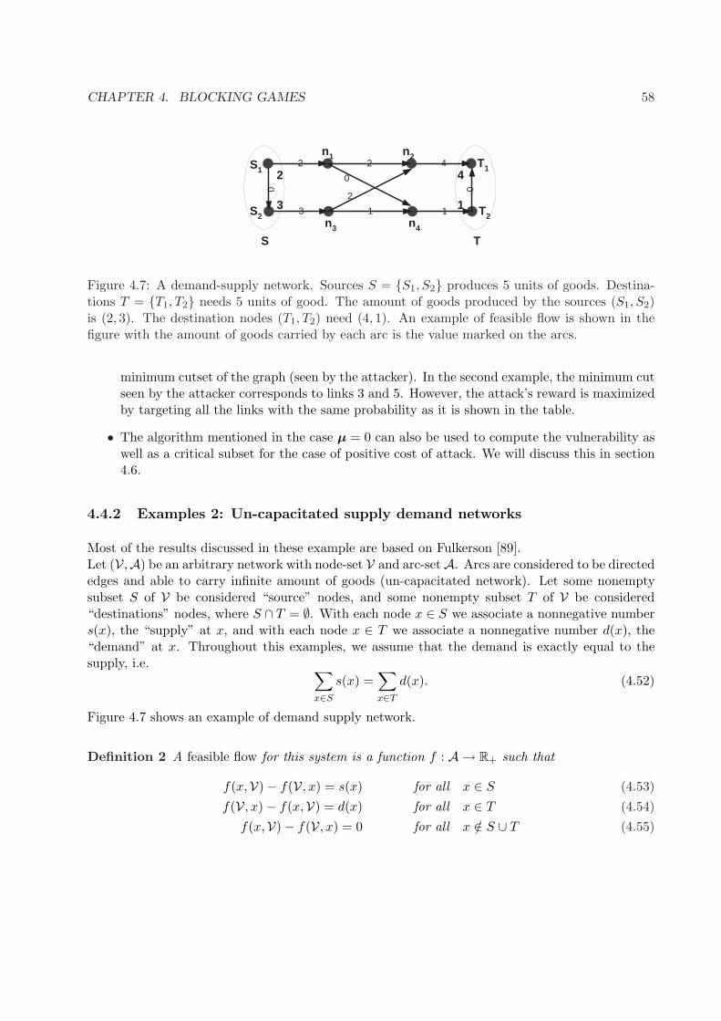
CHAPTER 4. BLOCKING GAMES 58
2
2
3
4
1
2
1
S 1
S 2 T 2
T 1
n 1 n 2
n 3 n 4
2
3
4
1
0 0
0
S T
Figure 4.7: A demand-supply network. Sources S = S1, S2 produces 5 units of goods. Destina-tions T = T1, T2 needs 5 units of good. The amount of goods produced by the sources (S1, S2)is (2, 3). The destination nodes (T1, T2) need (4, 1). An example of feasible flow is shown in thefigure with the amount of goods carried by each arc is the value marked on the arcs.
minimum cutset of the graph (seen by the attacker). In the second example, the minimum cutseen by the attacker corresponds to links 3 and 5. However, the attack’s reward is maximizedby targeting all the links with the same probability as it is shown in the table.
• The algorithm mentioned in the case µ = 0 can also be used to compute the vulnerability aswell as a critical subset for the case of positive cost of attack. We will discuss this in section4.6.
4.4.2 Examples 2: Un-capacitated supply demand networks
Most of the results discussed in these example are based on Fulkerson [89].Let (V,A) be an arbitrary network with node-set V and arc-setA. Arcs are considered to be directededges and able to carry infinite amount of goods (un-capacitated network). Let some nonemptysubset S of V be considered “source” nodes, and some nonempty subset T of V be considered“destinations” nodes, where S ∩ T = ∅. With each node x ∈ S we associate a nonnegative numbers(x), the “supply” at x, and with each node x ∈ T we associate a nonnegative number d(x), the“demand” at x. Throughout this examples, we assume that the demand is exactly equal to thesupply, i.e. ∑
x∈S
s(x) =∑
x∈T
d(x). (4.52)
Figure 4.7 shows an example of demand supply network.
Definition 2 A feasible flow for this system is a function f : A → R+ such that
f(x,V)− f(V, x) = s(x) for all x ∈ S (4.53)f(V, x)− f(x,V) = d(x) for all x ∈ T (4.54)
f(x,V)− f(V, x) = 0 for all x /∈ S ∪ T (4.55)

CHAPTER 4. BLOCKING GAMES 59
We let F denotes the set of feasible flows.
In other terms, a feasible flow is an assignment of values to the arcs that satisfies the conservationof flow. In Figure 4.7, a feasible flow is shown on the arcs of the graph.In the equations above, f(x,V) denotes
f(x,V) =∑
y∈V|(x,y)∈Af(x, y) (4.56)
We will also use the following notations for arbitrary X ⊆ V, Y ⊆ V.
(X, Y ) = (x, y) ∈ A | x ∈ X, y ∈ Y , (4.57)
and if g is any real-valued function defined on the arcs,
g(X, Y ) =∑
(x,y)∈(X,Y )
g(x, y). (4.58)
All data (i.e. supplies and demands) are assumed to be integers and we only consider integralfeasible flows.
To put this example in the context of the blocking game, we assume that a network manager(defender) is choosing a set of arcs on which to carry positive amount of goods. To determine theamount of goods on each selected arc, we add the constraints of conservation of flows so that thedefender’s choice is restricted to the set of feasible flows. The defender would like to select a set ofarcs (feasible flow) to maximize the amount of goods transferred from a set of sources to a set ofdestinations. We let f(a) be the quantity of goods that flow f carries on arc a.
An attacker is selecting an arc to attack in order to minimize the amount of goods transferred.The attacker pays a cost µ(a) to successfully disrupt the transport on arc a. She also has theoption of not attacking. If flow f is selected and arc a is targeted, the defender loses f(a) and theattacker gets f(a)− µ(a).
We model this interaction as a game and consider mixed strategy Nash equilibria where theattacker chooses a distribution (αf , f ∈ F) on the set F of feasible flows, and the attacker, adistribution (βa, a ∈ A) on the A of arcs. The model and results in sections 4.2 and 4.3 can beused to analyze the game.
Remark:Since flows are mostly seen as functions (rather than vectors), we have adopted the ‘functionnotation’ in these examples. We will also keep the usual network flow notation: f to designate aflow and a for an arc. For instance, instead of the math-bold (λT,e) to designate the payoff of thechoice pair (T, e), we will use f(a) to refer to the payoff of the game when the defender chooses thefeasible flow f and the attacker the arc a. We have also preferred F and A to T and E to designatethe sets of flows and arcs. Also, we use F to denote the payoff matrix (which used to be Λ).

CHAPTER 4. BLOCKING GAMES 60
The Flow polyhedron PF and its blocker bl(PF )
Let F be the matrix whose columns are indexed by the arcs of the network and whose rows areindexed by the integral feasible flows, with entry f(a) representing the amount that flow f assignedto arc a‡‡. Let PF be the polyhedron associated with F . We are interested in characterizing PF
and its blocker bl(PF ).
The following theorem by Fulkerson and Weinberger [89] describes the polyhedron PF and givesthe generator matrix of its blocker bl(PF ).
Theorem 5 Let F be the matrix of integral feasible flows in an un-capacitated supply-demandnetwork (V,A) with integral-valued supply and demand functions, s(·) and d(·), respectively. Thenthe polyhedron PF is described by
PF =
x ∈ R|A|+ |
∑
a∈(X,X)
xa ≥ d(X)− s(X), ∀X ⊆ V s.t. d(X)− s(X) ≥ 1
. (4.59)
Here, d(X) is the total demand of the nodes in X, and s(X) is the corresponding total supply;d(X)− s(X) is the excess demand in X.
This description tells that PF is the set of nonnegative vector x such that the sum of the entriesof x corresponding to links going from X ⊆ V to its complement X is greater than the excess ofdemand in X, for any X for which the excess demand in X is greater than 1 unit. In other words,a feasible flow should be able to compensate any excess of demand.
From the characterization above, Fulkerson and Weinberger [89] describe the blocker bl(PF ) asfollow. Let H be the matrix whose columns represent the arcs of the network, having a row ωX
for each X ⊆ V such that d(X)− s(X) ≥ 1. Set ωX(a) = 1/(d(X)− s(X)) for each arc a ∈ (X, X)and zero for other entries. Then, the essential rows of F and H form a blocking pair of matrices.Hence, the vertices of the blocking polyhedron are given by
ωX(a) =1
d(X)− s(X)1a∈(X,X), ∀a ∈ A, (4.60)
for all X ⊆ V verifying d(X)− s(X) ≥ 1. This implies that
ωX(A) =∑
a∈AωX(a) =
|(X, X)|d(X)− s(X)
, (4.61)
where |(X, X)| is the number of arcs going from X to X. Hence, we have that,
ωX(a)ωX(A)
=1a∈(X,X)
|(X, X)| ∀a ∈ A. (4.62)
‡‡Note that F may not be proper; also note that F may have no rows (if a feasible flow does not exist).

CHAPTER 4. BLOCKING GAMES 61
Applying the model
We can now write the expressions of λ(ωX) in (4.11), θ(ωX) in (4.12), and θ for this example. Wesimplify the notation and write λ(X) := λ(ωX), and θ(X) := θ(ωX).
The quantity λ(X) can be written as
λ(X) = minf
∑
a∈(X,X)
f(a)|(X, X)|
(4.63)
=minf
(∑a∈(X,X) f(a)
)
|(X, X)| (4.64)
=minf
(f(X, X)
)
|(X, X)| (4.65)
=M(X)|(X, X)| , (4.66)
where in the last equation, we have defined M(X) = minf
(f(X, X)
). It is the minimum amount
of goods that any feasible flow will carry on the arcs going from X to its complement X. Fromthis, we see that λ(X) is the minimum average flow per link going from X to X.
The vulnerability θ(X) of X ⊆ V is given by
θ(X) =M(X)|(X, X)| −
∑
a∈(X,X)
µa
|(X, X)| (4.67)
=M(X)|(X, X)| −
∑a∈(X,X) µa
|(X, X)| (4.68)
=M(X)|(X, X)| −
µ(X, X)|(X, X)| (4.69)
It is is the minimum average flow per link going from X to X minus the average cost of attackinglinks in (X, X).
A subset of nodes Xc is critical if
θ(Xc) = maxX⊆V:d(X)−s(X)≥1
(θ(X)) . (4.70)
We let θ (the vulnerability of the network) be the maximum value in the above equation, and wedefine Xc to be the set of all critical subsets of nodes.
Finally, the distribution βX(a) induced by (X, X) is given by
βX(a) =1a∈(X,X)
|(X, X)| , ∀a ∈ A (4.71)

CHAPTER 4. BLOCKING GAMES 62
Next, we illustrate the model and the results by some examples of demand-supply networks. Wewill separately consider the case where there is no cost of attack, and the case where the attacker“spends” a positive amount of effort to disrupt the network.
Nash equilibrium theorem for the supply-demand network game
Recall that
θ = maxX⊆V:d(X)−s(X)≥1
(M(X)− µ(X, X)|(X, X)|
). (4.72)
Applying Theorem 4 to the un-capacitated demand-supply game, we get the following.
1. If θ ≤ 0, then the attacker will opt to not launch an attack. The equilibrium strategy(αf , f ∈ F) for the defender is such that
∑
f∈Fαff(a) ≤ µ(a), ∀a ∈ A. (4.73)
The corresponding payoff is 0 for both players.
2. If θ ≥ 0, then for every probability distribution (γX , X ∈ Xc) on the set Xc of critical subsetsof nodes, the attacker’s strategy (β(a), a ∈ A) defined by
β(a) =∑
X∈Xc
γX
1a∈(X,X)
|(X, X)| (4.74)
is in Nash equilibrium with any strategy (αf , f ∈ F) of the defender that satisfies the followingproperties:
∑f∈F αff(a)− µ(a) = θ for all a ∈ A such that β(a) > 0.∑f∈F αff(a)− µ(a) ≤ θ for all a ∈ A.
(4.75)
Furthermore, there exists at least one such strategy α.
The corresponding payoffs are θ for the attacker, and r(γ) for the defender, where
r(γ) :=∑
X∈CγX
M(X)|(X, X)| . (4.76)
3. If µ = 0, then every Nash equilibrium pair of strategies for the game is of this type.

CHAPTER 4. BLOCKING GAMES 63
2
1
2
1
2
1
0 0 S T
n 1 n 2
n 3 n 4
3 3
(a) A demand-supply network with one source and onedestination. The total demand (supply) is 3. There aretwo critical subsets X = S and X = S, n1, n2, n3, n4which correspond to the 2 minimal cutsets of the network.The vulnerability of the network is 2.
2 3
1
2
1
0 1 S
T 2
T 1
n 1 n 2
n 3 n 4
4
3
1 2
(b) A demand-supply network with 2 bridges. Totaldemand (supply) is equal to 4. The critical subset isX = (S, n1, n2, n3, n4, T2) which corresponds to the bridge(n1, T1). The vulnerability of the network is equal to 3.
2 3
1
2
1
0 1 S
T 2
T 1
n 1 n 2
n 3 n 4
4
3
1
0
2
(c) Demand-Supply network with one additional routefrom T1 to T2. Total demand (supply) is equal to 4.There is only one bridge (n2, T1), whose corresponding setX = S, n1, n2, n3, n4, T2 is critical. The vulnerability isequal to 3.
2 3
1
2
1
0 1 S
T 2
T 1
n 1 n 2
n 3 n 4
4
3
1
0
2
(d) Demand-Supply chain with one additional route fromT2 to T1. Total demand (supply) is equal to 4. Thereis only one bridge (n4, T1), corresponding to subset X =S, n1, n2, n3, n4, T1. This set is not critical. There aretwo critical subsets: X = S and X = S, n1, n2, n3, n4.The vulnerability of the network is 2.
Figure 4.8: Illustrative demand-supply network examples. For each graph, a feasible flow is givenby the values on the arcs. The arcs (X, X) corresponding to critical subset X, are the dashed(dash-dotted) lines.

CHAPTER 4. BLOCKING GAMES 64
Examples and discussions: case case µ = 0
In these subsection, we assume that the attack cost µ is equal to zero so that a subset of verticesX ⊆ V is critical if it maximizes the ratio M(X)
|(X,X)| , where again M(X) = minf
(f(X, X)
).
• Let’s first consider a network flow problem with one source (S) and one destination (T ), andwhere the supply and demand functions are equal to 1: s(S) = d(T ) = 1. An example is thegraph in 4.8(a) with unit demand and supply.
In this case, any X ⊆ V that verifies d(X) − s(X) ≥ 1 must be an S-T cut. Indeed, if thesource is in X, then the destination cannot be in X (otherwise the difference d(X) − s(X)would have been zero), and vice-versa. Inversely, any S-T cut groups the nodes into twodisjoint sets; one containing S (say X) and the other containing T (X ). Also, since only oneunit of good is transferred from S to T , any feasible flow has to satisfy f(X, X) = 1 (onlyone unit is going across X and X). This implies that a subset Xc is critical if and only if
θ(Xc) = maxX⊆V:d(X)−s(X)≥1
(1
|(X, X)|)
= minX⊆V:d(X)−s(X)≥1
(|(X, X)|) . (4.77)
Thus, in this case, the critical subsets of nodes correspond to the S-T cuts of minimum sizei.e. the minimum cutsets.
In the NE of this game, the attacker’s mixed strategy equilibria are the convex combinationsof uniform attacks on the edges of the minimum cutsets. The defender’s strategy shouldsatisfy
∑f αf1f(a)>0 ≤ maxX
1
|(X,X)| , d(X)− s(X) ≥ 1
, for all arcs a ∈ A; and equalityholds for each arc a that is targeted with positive probability.
• Figure 4.8(a) shows a demand-supply network with one source and one destination. Thetotal demand is equal to the total supply and is equal to 3. The critical subsets of the graphX1 = S and X2 = S, n1, n2, n3, n4 correspond to its 2 minimum cutsets (shown in dashedand dash-dotted lines). The vulnerability of the graph is equal to θ = M(X)
|(X,X)| = 3/2.
The attacker’s mixed strategy Nash equilibria have the form γ 12(X1, X1)+(1−γ)1
2(X2, X2)∗.For example, γ = 1 gives a NE where the attacker targets each arc of the first minimum cutsetwith probability 1/2. The defender chooses a feasible flow with probability α such that thesum
∑f αff(a) is equal to 3
2 for each arc a that is attacked with positive probability; andfor any other arc, the sum is less than 3
2 .
• Consider the graphs shown in Figures 4.8(b), 4.8(c), and 4.8(d). In all these networks, thesource S produces 4 units of goods and destination T1 needs 3 units while T2 needs 1 unit.
The network in Figure 4.8(b) contains two bridges: destination T1 is reachable only via thearc (n2, T1), while access to T2 is only via arc (n4, T2). Since a bridge belongs to each path
∗In this compact notation, γ 12(X1, X1) means that each of the two links in (X1, X1) is attacked with probability
γ 12.

CHAPTER 4. BLOCKING GAMES 65
that reaches its corresponding destination, all bridges are a priori vulnerable links of thegraph. For instance (n2, T1) must carry any traffic going from X = S, n1, n2, n3, n4, T2 toX = T1. Since node T1 needs 3 units of goods, any flow will assign 3 units to arc (n2, T1).This implyies that M(X) = 3 and θ(X) = 3. This is the maximum vulnerability of thisnetwork implying that X = S, n1, n2, n3, n4, T2 is the critical subset of the network.
In all NE, the attacker attack arc (n2, T1) with probability 1, and the defender chooses treeaccording to a distribution α that satisfies:
∑f αff(a) ≤ 3 for all arcs a ∈ A. Equality is
satisfied on arc (n2, T1).
Figure 4.8(c) shows the same network as in the previous with one additional link from T1
to T2. The network now contains only one bridge (n2, T1). The same arguments used inthe previous example give that subset X = S, n1, n2, n3, n4, T2, corresponding to the onlybridge of the network, is the critical subset of the network. Its vulnerability is 3.
Compared to the previous case, we see that having an additional link (added in the waygiven here) does not yield to a stronger network. This suggests that if the defender wants tobenefit from adding a new link to the network, he has to determine a proper way to do it.An arbitrary addition of link might not provide any benefit.
In the graph shown in Figure 4.8(d) the additional links goes from T2 to T1. The networkstill contains a bridge because the only way to reach T2 is via (n4, T2). However, that bridgeis not a critical link. The most vulnerable arcs are the ones going from the critical subsetX = S to X, and those going from the critical subset X = S, n1, n2, n3, n4 to X.
In fact, since bridge (n4, T2) (corresponding to X1 = S, n1, n2, n3, n4, T1) is the only way toreach T2, any feasible flow will assign positive load to that arc. The minimum amount of trafficcarried over (n4, T2) on any feasible flow is equal to 1. Thus, M(X1) = 1 and θ(X1) = 1.On the other hand, if X = S, any feasible flow will carry the total amount of goods on thearcs (X, X). As a consequence, M(X) = 4 and the vulnerability θ(X) = 4/2 = 2. The is themaximum vulnerability implying that X is critical. Similarly, subset X = S, n1, n2, n3, n4is critical.
Adding the extra link in the way described here, strictly decreases the vulnerability of thenetwork (as opposed to the previous case where the additional link was not optimally added).This phenomenon was already observe in the spanning tree game. It illustrates the importanceof knowing the critical sets when designing a network topology.
• As was mentioned earlier, M(X) is the minimum amount of goods that any feasible flowwill carry from X to its complement. For any target subset of nodes X, the defender istrying to find a feasible flow that achieves this minimum. The attacker is choosing a subsetX that maximizes the fraction M(X)
|(X,X)| . In other words, the attacker chooses a subset X
that maximizes the minimum average traffic per link from X to X. This maximum can beachieved by targeting set of edges that separate all sources to all destinations. This is thecase in Figures 4.8(a) and 4.8(d) where for example the edges going from S to the rest of thenetwork are critical. The maximum can also be achieved by attacking edges that separate a

CHAPTER 4. BLOCKING GAMES 66
given set of destination nodes to the rest of the network as is the case in examples 4.8(b) and4.8(c).
Examples and discussions: case case µ > 0
Now we assume that the attack cost µ is a positive vector. The networks in Figures 4.9 illustratethis case. In all networks, the values of the attack costs are placed close to the corresponding arcs.
In Figure 4.9(a) the costs of attack are relatively high. The vulnerability θ of the network isequal to −1/2 and is achieved by subsets X = S (dash-dotted lines) and X = S, n1, n2, n3, n4(dashed lines). Since θ < 0, the attacker will not launch an attack. The defender needs to choosefeasible flows according to a distribution α that satisfies
∑
f
αff(a) ≤ µ(a), ∀ a ∈ A. (4.78)
We know from the theorem that such distribution exists.
It is worth noting that although the network contains a bridge (link (n4, T2)), the attacker willnot attack (even not the bridge). In fact, in this example, the cost of successfully attacking thebridge (which is 2) is greater than the reward that the attacker expects from such attack (which isequal to 1).
Figure 4.9(b) is an example of network with vulnerability zero. This maximum vulnerability isachieved at X = S (dash-dotted lines) and X = S, n1, n2, n3, n4, T2 (dashed lines). A certainnumber of interesting phenomenon happen in this example.
First, the bridge (n4, T2) is so costly that it is not part of the edges induced by any critical subsetof nodes. The are two critical subsets and each will lead to an zero average attack reward for theattacker. An attack that focuses on the links going from X = S to X is preventing the traffic toreach the destinations, without any distinction of the destinations. It results to an average attackloss of M(X)
|(X,X)| = 42 = 2 for the defender, and in average 2 units of goods will reach the destinations.
An attack that focuses on the edges entering T1 (dashed lines) is preventing traffic to reach T1. Theaverage loss of such attack is M(X)
|(X,X)| = 32 , and an average of 2.5 units of goods will always reach
the destinations; 1 unit of it will always go to node T2.
This phenomenon was already seen in the spanning tree game. Although the attacks give thesame payoff to the attacker, their impacts on the defender are different. One interesting relatedquestion is which equilibrium will be played, or how can the defender force the second equilibriumwhich is clearly better for him. Our model does not permit the study of equilibrium selection.Other inputs and parameters need to be considered to answer to those questions.
Figure 4.9(c) is an example of network with positive vulnerability. The network also contains asingle critical subset X = S, n1, n2, n3, n4 and its vulnerability is equal to 1. The attacker willattack the two links in (X, X) each with probability 1/2. Her average net reward is 1. The defender

CHAPTER 4. BLOCKING GAMES 67
will choose feasible flows according to a distribution α that satisfies∑
f
αff(a)− µ(a) = θ, ∀ a ∈ (X, X) (4.79)
∑
f
αff(a)− µ(a) ≤ θ, ∀ a ∈ A. (4.80)
The average attack loss is equal to 2 and in average 2 units of goods will reach the destinations.
4.5 Proof of the NE Theorem
In this section we provide a proof of the Nash equilibrium theorem presented in section 4.3.
4.5.1 “No Attack” Option
We start by showing that if θ ≤ 0 “No Attack” and α verifying (4.14) are best responses to eachother.
Best Responses
First, notice that if the attacker chooses “No Attack”, then any α will result to the minimum lossof zero for the defender (in particular the one given in the theorem). Now, assume that α satisfies(4.14). Then, “No Attack” is a dominant strategy for the attacker. In fact, the expected attackreward is
R(α, β) =∑
e∈E
β(e)(λα(e)− µ(e)
), (4.81)
which is less than zero if λα(e) − µ(e) ≤ 0, ∀ e ∈ E , and for any β. On the other hand, zeroreward can always be achieved by playing e∅. As a consequence, not attacking is a best responseto α satisfying (4.14).
Existence of the Equilibrium Distribution α
Now, we need to prove the existence of a distribution α that satisfies (4.14) whenever θ ≤ 0. Tosummarize, we are looking for α verifying:
α :
α ≥ 01′T α = 1Λ′α ≤ µ,
(4.82)
We first show the following lemma.

CHAPTER 4. BLOCKING GAMES 68
S
T 2
T 1
n 1 n 2
n 3 n 4
4
3
1
2
3
3
3
2
2
3
2
1
(a) Example of demand/supply network with high attackcosts. The vulnerability of the network is −1/2 and theattacker does not launch an attack. Two subsets achievethe maximum vulnerability of −1/2. The correspondingedges are shown in dashed and dash-dotted.
S
T 2
T 1
n 1 n 2
n 3 n 4
4
3
1
3
1
3
3
3
2
2
3
1
(b) Example of demand/supply network with attack coststhat give zero payoff to the attacker. Vulnerability is 0, andcorresponding critical set are shown in dashed and dash-dotted.
S
T 2
T 1
n 1 n 2
n 3 n 4
4
3
1
1
2
2
1
1
1
1
1
3
(c) Example of demand/supply with positive cost of attackand positive vulnerability. There is only one critical subsetshown by the dashed line. The vulnerability of the networkis 4−2
2= 1.
Figure 4.9: Illustrative demand-supply network examples for µ > 0. For each graph, the value ofthe attack cost is marked close to the arc. The arcs (X, X) corresponding to critical subset X, arethe dashed (dash-dotted) lines.

CHAPTER 4. BLOCKING GAMES 69
Lemma 4θ ≤ 0 ⇒ µ ∈ PΛ. (4.83)
Proof: For this we show that if θ ≤ 0, then µ′ω ≥ 1, for any vertex ω of bl(PΛ). As a result ofthis, µ belongs to the blocker of bl(PΛ) which is PΛ.
If θ ≤ 0, then we have that, for all ω ∈ Ω,
∑
e∈E
ω(e)ω(E)
µ(e) ≥ minT∈T
(∑
e∈E
ω(e)ω(E)
λT,e
). (4.84)
Or, equivalently
µ′ω ≥ minT∈T
(∑
e∈Eω(e)λT,e
), for all ω ∈ Ω. (4.85)
Now, since ω ∈ bl(PΛ) we have that∑
e∈Eω(e)λT,e ≥ 1, (4.86)
which implies that µ · ω ≥ 1, ∀ ω ∈ Ω, or equivalently µ ∈ PΛ.Using Lemmas 1 and 4, we conclude that the value of the following LP is greater than 1.
Maximize 1T x
subject to Λ′x ≤ µ, and x ≥ 0 (4.87)
Construct α satisfying (4.14) by normalizing any solution of this LP.
4.5.2 The “Always Attack” option
As in the previous section, we will first argue that the strategies given in the theorem are bestresponses to each other, then we show the existence of a distribution (αT , T ∈ T ) that satisfies(4.16). We start by the following lemma.
Lemma 5 If θ > 0, then “No Attack” is a strictly dominated strategy for the attacker.
Note that if θ ≥ 0, all the steps of the proof still hold. However, “No Attack” will only be weaklydominated, and as seen in the previous case, there will exist equilibrium for which the attacker willopt to not launch an attack. In other words, if θ = 0 there exist equilibria for which βe∅ = 1, aswell as equilibria for which βe∅ = 0.
Proof: Suppose that ω ∈ Ωmax is a critical vertex of bl(PΛ) and let β = (ω(e)ω(E) , e ∈ E). We will
show that the attacker can achieve positive reward by playing β (independently of α). To see this,

CHAPTER 4. BLOCKING GAMES 70
first notice that since θ(ω) = θ > 0 for all ω ∈ Ωmax, we have that
λ(ω) = minT∈T
(∑
e∈E
ω(e)ω(E)
λT,e
)>
∑
e∈E
ω(e)ω(E)
µ(e) =µ′ωω(E)
(4.88)
Playing the strategy β, the attacker’s expected reward against any defense strategy α is given by
R(α, β) =∑
e∈E
ω(e)ω(E)
(∑
T∈TαT λT,e − µ(e)
)
=∑
T∈TαT
(∑
e∈E
ω(e)ω(E)
λT,e −∑
e∈E
ω(e)ω(E)
µ(e)
)(4.89)
≥∑
T∈TαT
(λ(ω)−
∑
e∈E
ω(e)ω(E)
µ(e)
)(4.90)
=∑
T∈TαT
(λ(ω)− µ′ω
ω(E)
)(4.91)
= λ(ω)− µ′ωω(E)
(4.92)
> 0, (4.93)
where in (4.90) we use the definition of λ(ω); (4.93) is implied by (4.88).
As a consequence of this lemma, we conclude that if θ > 0, then the attacker will never play the“No Attack” (i.e. e∅) strategy.
Best Responses
Given the set of critical vertices Ωmax and α satisfying (4.16), any distribution β of the formβ(e) =
∑ω∈Ωmax
γωω(e)ω(E) for some distribution γ = (γω, ω ∈ Ωmax), achieves a reward of θ. This
is the maximum possible reward that the attacker can get. To see this, observe that for any β,
R(α, β) =∑
e∈Eβ(e)
(λα(e)− µ(e)
) ≤∑
e∈Eβ(e)θ ≤ θ. (4.94)

CHAPTER 4. BLOCKING GAMES 71
The upper bound of θ is achieved by any β = (ω(e)ω(E) , e ∈ E) and ω ∈ Ωmax, because for any such β,
R(α, β) =∑
e∈E
ω(e)ω(E)
(∑
T∈TαT λT,e − µ(e)
)(4.95)
=∑
T∈TαT
(∑
e∈E
ω(e)ω(E)
λT,e −∑
e∈E
ω(e)ω(E)
µ(e)
)(4.96)
≥∑
T∈TαT
(λ(ω)−
∑
e∈E
ω(e)ω(E)
µ(e)
)(4.97)
=∑
T∈TαT θ (4.98)
= θ, (4.99)
where (4.97) uses the definition of λ(ω), and in (4.98) we use the fact that ω ∈ Ωmax.As a consequence, any distribution of the form (ω(e)
ω(E) , e ∈ E) for ω ∈ Ωmax is a best response andany convex combination of those distributions is also a best response.
Now assume that β is given as in (4.15) for some distribution (γω, ω ∈ Ωmax). Then, thedistribution (αT , T ∈ T ) in (4.16) achieves a loss of r(γ) =
∑ω∈Ωmax
γωλ(ω). This is theminimum possible loss. To see this, note that, for any α, the expected loss seen by the defender isgiven by
L(α,β) =∑
T∈TαT
(∑
e∈Eβ(e)λT,e
)(4.100)
=∑
T∈TαT
(∑
e∈E
( ∑
ω∈Ωmax
γωω(e)ω(E)
)λT,e
)(4.101)
=∑
T∈TαT
( ∑
ω∈Ωmax
γω
(∑
e∈E
ω(e)ω(E)
λT,e
))(4.102)
≥∑
T∈TαT
( ∑
ω∈Ωmax
γωλ(ω)
)(4.103)
=∑
T∈TαT r(γ) (4.104)
= r(γ). (4.105)
The lower bound r(γ) can be achieved by choosing α such that∑
T∈T αT λT,e = θ + µ(e) for eache ∈ E such that β(e) > 0 (the existence of such α is shown in the second part of the theorem).

CHAPTER 4. BLOCKING GAMES 72
This can be seen by rewriting L(α, β) as
L(α,β) =∑
e∈Eβ(e)
(∑
T∈TαT λT,e
)(4.106)
=∑
e∈Eβ(e) (θ + µ(e)) (4.107)
= θ + β′µ = r(γ). (4.108)
The last equality above is justified by
θ + β′µ = θ +∑
ω∈Ωmax
γω
(1
ω(E)ω′µ
)− r(γ) + r(γ) (4.109)
= θ +∑
ω∈Ωmax
γω
(1
ω(E)ω′µ− λ(ω)
)+ r(γ) (4.110)
= θ +∑
ω∈Ωmax
γω (−θ) + r(γ) (4.111)
= θ − θ + r(γ) (4.112)= r(γ), (4.113)
where in (4.109) and (4.110) we use the definitions of β and r(γ) respectively and write the sum-mation over E as a product of a row vector and a column vector. In 4.110 we have also used thedefinition of θ(ω) for a critical vertex ω ∈ Ωmax.
From this analysis, we see that for the set Ωmax of critical vertices, the distributions given in thetheorem are best responses to each other, as a consequence, they form a Nash equilibria under theassumption that α exists. Such existence is shown in the next section.
Existence of the Equilibrium Distribution α
We claim that for any (β(e), e ∈ E) of the form in the statement (4.15) of Theorem 4, we can findan associated (αT , T ∈ T ) of the form (4.16).
Theorem 6 Assume that θ ≥ 0 and let Ωmax be the set of critical vertices. Let x∗ be the solutionof the following LP:
Maximize 1′T x
subject to A′x ≤ b, x ≥ 0. (4.114)
where b = θ(E)1E + µ. Then,
a) 1′T x∗ ≤ 1;

CHAPTER 4. BLOCKING GAMES 73
b) 1′T x∗ ≥ 1;
c) A′x∗(e) = b(e),∀e ∈ E for which β(e) > 0.
As a consequence, x∗ satisfies (4.16) and implies the existence of α.
Proof: a) To prove that 1′T x∗ ≤ 1, we first observe that
β′Λ′x =∑
T∈TxT
(∑
e∈Eβ(e)λT,e
)(4.115)
=∑
T∈TxT
(∑
e∈E
( ∑
ω∈Ωmax
γωω(e)ω(E)
)λT,e
)(4.116)
=∑
T∈TxT
( ∑
ω∈Ωmax
γω
(∑
e∈E
ω(e)ω(E)
λT,e
))(4.117)
≥∑
T∈TxT
( ∑
ω∈Ωmax
γωλ(ω)
)(4.118)
=∑
T∈TxT r(γ) (4.119)
= r(γ)1′T x (4.120)
On the other hand, from the constraints Λ′x ≤ b = θ1E + µ and from (4.113), we have that
β′Λ′x ≤ β′ (θ1E + µ) = θ + β′µ = r(γ) (4.121)
Combining (4.120) and (4.113) it follows that,
r(γ)1′T x ≤ β′Λ′x ≤ r(γ) (4.122)
Thus 1′T x ≤ 1 for all feasible x, i.e. the value of the program is at most 1.

CHAPTER 4. BLOCKING GAMES 74
b) To prove that 1TT x∗ ≥ 1, we use Lemma 1 above to claim that it suffices to verify that the
vector b belongs to the polyhedron PΛ. For that, we will show that b′ω ≥ 1 for all ω ∈ Ω. In fact∗,
ω′b = θω′1E + ω′µ (4.123)
= ω(E)(
θ +1
ω(E)ω′µ
)(4.124)
≥ ω(E)(
λ(ω)− 1ω(E)
ω′µ +1
ω(E)ω′µ
)(4.125)
= ω(E)λ(ω) (4.126)
= ω(E) minT∈T
(∑
e∈E
ω(e)ω(E)
λT,e
)(4.127)
= minT∈T
(∑
e∈Eω(e)λT,e
)(4.128)
≥ 1 (4.129)
where (4.129) follows from the fact that ω ∈ bl(PΛ). Indeed, if ω ∈ bl(PΛ), then by definitionof the blocker polyhedron,
∑e∈E ω(e)λT,e ≥ 1 for all T ∈ T . Thus, we have that Ωb ≥ 1, which
implies that b belongs to the blocker of bl(PΛ) which is equal to PΛ.
Now, using Lemma 1, we conclude that the value of the LP is greater than 1.This, together with the previous part a) imply that the value of the LP is equal to 1; hence, anysolution x∗ is a probability distribution on T .
c) We first observe from (4.120) and (4.113) that
β′Λ′x∗ = r(γ)1T x∗ = r(γ). (4.130)
Also, Λ′x∗ ≤ θ1E + µ by the constraints of the primal LP above.Now, assume that Λ′x∗(e) < θ + µ(e) for some e ∈ E with β(e) > 0. Then,
β′Λ′x∗ =∑
e∈Eβ(e)Λ′x∗(e) (4.131)
<∑
e∈Eβ(e)(θ + µ(e)) (4.132)
= θ +∑
e∈Eβ(e)µ(e) (4.133)
= r(γ), (4.134)
where the last equality is obtained by using the same arguments as in (4.109)-(4.113). This con-tradicts observation (4.130). As a consequence, Λ′x∗(e) = θ + µ(e) for all e ∈ E with β(e) > 0.
This ends the proof of the theorem and establishes the existence of an α satisfying (4.16) for anyβ defined as in (4.15).
∗Again we use vector product for summation.
CHAPTER 4. BLOCKING GAMES 75
4.5.3 Enumerating all Nash Equilibria
In this section, we consider the zero-sum game where µ = 0. In this case, since there is no cost ofattack θ > 0. We will show that for any strategy pair (αT , T ∈ T ) and (β(e), e ∈ E) that are inNash equilibrium, it must be the case that (β(e), e ∈ E) is given by
β(e) =∑
ω∈Ωmax
γωω(e)ω(E)
, (4.135)
for some probability distribution (γω,ω ∈ Ωmax).As a consequence of this, we will conclude that α must be in the form given in the Nash equilibriumtheorem.
First, notice that since µ = 0, we have that λ(ω) = θ(ω) (see the definitions in (4.12) and (4.11)).Next, we use the zero-sum structure of the game to observe that it has a well-defined value, which,by the second part of Theorem 4, is equal to,
θ = maxω∈Ω
(λ(ω)) = maxω∈Ω
(minT∈T
(∑
e∈E
ω(e)ω(E)
λT,e
)). (4.136)
Thus, we must have that, for any Nash equilibrium pair (α, β),
θ =∑
T∈T
∑
e∈EαT β(e)λT,e =
∑
T∈TαT
(∑
e∈Eβ(e)λT,e
)> 0. (4.137)
From the above equation we can argue that there exists a scaling factor κ > 0 such that (κβ(e), e ∈E) belongs to the blocker bl(PΛ), or equivalently,
∑
e∈Eκβ(e)λT,e ≥ 1, for all T ∈ T . (4.138)
In fact, by letting αmax be the maximum αT , and defining κ = Nαmaxθ , then (κβ(e), e ∈ E) verifies
(4.138). We let κ denote the smallest such scaling that works among all scalings κ > 0.
Also, observe that since κ is the smallest nonnegative scaling of (β(e), e ∈ E) such that (κβ(e), e ∈E) belongs to bl(PΛ), there must exist some To ∈ T for which
∑e∈E κβ(e)λTo,e = 1.
Indeed this is the case because since κβ ∈ bl(PΛ), we have that∑
e∈E κβ(e)λT,e ≥ 1 for all T ∈ T .If this inequality were strict for all T ∈ T , then considering the strategy Tmin that minimizes thesum
∑e∈E κβ(e)λT,e over all T , we can construct
κ =κ∑
e∈E β(e)λTmin,e. (4.139)
κ verifies κ < κ and κβ ∈ bl(PΛ). This contradicts the assumption that κ was the smallest such κ.
Now, we claim that:

CHAPTER 4. BLOCKING GAMES 76
Lemma 6 If (αT , T ∈ T ) and (β(e), e ∈ E) form a NE of the game, then we can write
κβ(e) =∑
ω∈Ω
γωω(e)
ω(E)λ(ω), (4.140)
for some probability distribution (γω, ω ∈ Ω).
We delay the proof of this lemma for later.
Using this expression of κβ, we can write the value of the game θ as:
θ =1κ
∑
T∈TαT
(∑
e∈Eκβ(e)λT,e
)(4.141)
=1κ
∑
T∈TαT
(∑
e∈E
( ∑
ω∈Ω
γωω(e)
ω(E)λ(ω)
)λT,e
)(4.142)
=1κ
∑
T∈TαT
( ∑
ω∈Ω
γω
(1
λ(ω)
∑
e∈E
ω(e)ω(E)
λT,e
))(4.143)
≥ 1κ
∑
T∈TαT
( ∑
ω∈Ω
γω
)(4.144)
=1κ
, (4.145)
where in (4.144) we use the fact that λ(ω) ≤ ∑e∈E
ω(e)ω(E)λT,e for all T ∈ T .
Now, since (α, β) is a Nash equilibrium pair, the expression∑
e∈E β(e)λT,e is minimal for eachT ∈ T for which αT > 0. Furthermore, this minimum value is equal to θ. From this, we get that,
θ = minT∈T
(∑
e∈Eβ(e)λT,e
)(4.146)
=1κ
minT∈T
(∑
e∈Eκβ(e)λT,e
)(4.147)
≤ 1κ
, (4.148)
where in (4.148) we use the fact that the minimum in (4.147) is less than∑
e∈E κβ(e)λTo,e, which,by definition, is equal to 1. Thus, θ = 1
κ .

CHAPTER 4. BLOCKING GAMES 77
This, combined with (4.140) that we sum over e ∈ E , imply:
1θ
= κ =∑
e∈Eκβ(e) (4.149)
=∑
e∈E
∑
ω∈Ω
γωω(e)
ω(E)λ(ω)(4.150)
=∑
ω∈Ω
γω1
ω(E)λ(ω)
∑
e∈Eω(e) (4.151)
=∑
ω∈Ω
γω1
λ(ω). (4.152)
Now, recalling (4.136) that θ = maxω∈Ω (λ(ω)), we conclude that γω can be nonzero only forω ∈ Ω that satisfies λ(ω) = maxω∈Ω (λ(ω)). In other terms, γω > 0 only for ω ∈ Ωmax.Hence, we can write
β(e) =∑
ω∈Ωmax
γωω(e)ω(E)
. (4.153)
The last thing that remains to be shown to complete the proof of the theorem is that if (αT , T ∈T ) and (β(e), e ∈ E) are in Nash equilibrium and (β(e), e ∈ E) is of the form (4.15) in the statementTheorem 4, then (αT , T ∈ T ) must also be of the form in the statement (4.16) of the theorem.We have already shown that for (β(e), e ∈ E) of the form (4.15), we must have for every strategy(αT , T ∈ T )
∑
T∈TαT
∑
e∈Eβ(e)λT,e =
∑
T∈TαT
(∑
e∈E
( ∑
ω∈Ωmax
γωω(e)ω(E)
λT,e
))(4.154)
=∑
T∈TαT
( ∑
ω∈Ωmax
γω
(∑
e∈E
ω(e)ω(E)
λT,e
))(4.155)
≥∑
T∈TαT
( ∑
ω∈Ωmax
γωθ
)(4.156)
= θ, (4.157)
where (4.156) follows from (4.136). The minimum value of θ can be achieved by choosing α suchthat
∑T∈T αT λT,e = θ whenever β(e) > 0. To see that, rewrite the summation as
∑
T∈TαT
∑
e∈Eβ(e)λT,e =
∑
e∈Eβ(e)
(∑
T∈TαT λT,e
), (4.158)
and observe the claim.

CHAPTER 4. BLOCKING GAMES 78
The existence of such α has been shown in the previous section. It also has been shown thatsuch α is a best response to (β(e), e ∈ E). For β to be a best response to α (hence, the (α,β) pairto be in Nash equilibrium), α must also satisfy
∑
T∈TαT λT,e ≤ θ for all e ∈ E . (4.159)
Suppose, on the contrary, that this is not the case (i.e. there is some e ∈ E for which∑
T∈T αT λT,e >θ). Then the attacker will prefer to switch to playing strategy e with probability 1 and receive higherreward. This violates the assumption that (αT , T ∈ T ) and (β(e), e ∈ E) are in Nash equilibrium.Thus, α satisfies (4.159). This completes the proof of the theorem, provided that the claim inLemma 6 can be justified. We give a proof of the lemma in the next section.
Proof of Lemma 6
The claim is that if (αT , T ∈ T ) and (β(e), e ∈ E) are in Nash equilibrium, and if κ > 0 denotesthe smallest κ > 0 for which (κβ(e), e ∈ E) ∈ bl(PΛ), then we must have
κβ(e) =∑
ω∈Ω
γωω(e)
ω(E)λ(ω), (4.160)
for some probability distribution (γω,ω ∈ Ω).
Indeed, this needs a proof, because a priori we only know that we can write
κβ(e) =∑
ω∈Ω
γωω(e)
ω(E)λ(ω)+ v(e), (4.161)
for some probability distribution (γω, ω ∈ Ω) and some (v(e), e ∈ E) such that v(e) ≥ 0 for alle ∈ E .
We now provide the proof that works as follow. We consider the expression of this form for(κβ(e), e ∈ E) for which v(E) :=
∑e∈E v(e) is as small as possible. We will assume that v(E) > 0
for this expression, and arrive at a contradiction.Note that we must have v(E) < κ for this expression, i.e. there has to be a nontrivial “convex hullpart”.
CHAPTER 4. BLOCKING GAMES 79
First observe that for all T ∈ T , we have∑
e∈Eβ(e)λT,e =
1κ
∑
e∈Eκβ(e)λT,e (4.162)
=1κ
∑
e∈E
( ∑
ω∈Ω
γωω(e)
ω(E)λ(ω)+ v(e)
)λT,e (4.163)
=1κ
∑
ω∈Ω
γω
(1
λ(ω)
∑
e∈E
ω(e)ω(E)
λT,e
)+
1κ
∑
e∈Ev(e)λT,e (4.164)
≥ 1κ
∑
ω∈Ω
γω +1κ
vλ(T ) (4.165)
=1κ
+vλ(T )
κ, (4.166)
where in (4.165) we use the definition of λ(ω), and define vλ(T ) :=∑
e∈E v(e)λT,e. As a consequence,we have that
minT∈T
(∑
e∈Eβ(e)λT,e
)≥ 1
κ+ min
T∈T
(vλ(T )
κ
)(4.167)
Next, observe that since (αT , T ∈ T ) and (β(e), e ∈ E) are in Nash equilibrium, it must be thecase that
∑e∈E β(e)λT,e is the same for every T ∈ T such that αT > 0. Also, by the same reasoning
as in (4.148), we have that for all such T
∑
e∈Eβ(e)λT,e = min
T∈T
(∑
e∈Eβ(e)λT ,e
)≤ 1
κ. (4.168)
This, combined with (4.159), implies that minT∈T(∑
e∈E β(e)λT,e
)= 1
κ and that vλ(T ) = 0 for allT ∈ T such that αT > 0.
Now, let
β(e) :=1
κ− v(E)
∑
ω∈Ω
γωω(e)
ω(E)λ(ω). (4.169)
This quantity satisfies∑
(e)β(e) = 1 and β(e) ≥ 0 for all e ∈ E . Thus, (β(e), e ∈ E) is a probabilitydistribution on E , and can be used as a strategy by the attacker. This can be verified by summingboth sides of (4.161) over e ∈ E to get,
κ =∑
e∈Eκβ(e) =
∑
e∈E
( ∑
ω∈B
γωω(e)
ω(E)λ(ω)+ v(e)
)(4.170)
=∑
e∈E
( ∑
ω∈B
γωω(e)
ω(E)λ(ω)
)+ v(E) (4.171)
= (κ− v(E))∑
e∈Eβ(e) + v(E). (4.172)

CHAPTER 4. BLOCKING GAMES 80
This last equation implies that ∑
e∈Eβ(e) =
κ− v(E)κ− v(E)
= 1. (4.173)
For this strategy (β), in response to (αT , T ∈ T ), the attack reward is at least 1κ−v(E) . In fact,
∑
T∈TαT
∑
e∈Eβ(e)λT,e =
∑
T∈TαT
(∑
e∈E
(1
κ− v(E)
∑
ω∈Ω
γωω(e)
ω(E)λ(ω)
)λT,e
)(4.174)
=1
κ− v(E)
∑
T∈TαT
( ∑
ω∈Ω
γω1
λ(ω)
(∑
e∈E
ω(e)ω(E)
λT,e
))(4.175)
≥ 1κ− v(E)
∑
T∈TαT
∑
ω∈Ω
γω (4.176)
=1
κ− v(E). (4.177)
However, because of the fact that v(T ) = 0 for all T ∈ T for which αT > 0, the benefit obtainedby the attacker by playing the NE strategy (β(e), e ∈ E) is only 1
κ , which is strictly smaller than1
κ−v(E) under the standing assumption that v(E) > 0. As a consequence, if v(E) > 0, the attacker
can be better off by changing her strategy to β. But this contradicts the assumption that (α,β)form a NE. Thus, v(E) = 0 implying that v(e) = 0 for all e ∈ E as we wanted to show.
4.6 Algorithm to Compute θ and a Critical Vertex
In this section, we show how one can derive an algorithm to compute the vulnerability θ of thegame, as well as a maximizing (hence critical) vertex.We will consider that the cost µ is equal to0. The case of non-zero µ can be analyzed using the same techniques.
Recall that if µ = 0,
θ = maxω∈Ω
(M(ω)ω(E)
), (4.178)
where Ω is the matrix having as rows the vertices ω of blocking polyhedron bl(PΛ) . The functionM(·) is defined as
M(ω) = minT∈T
∑
e∈EωeλT,e. (4.179)
The algorithm is inspired by Cunningham [87] who used it in a none-game theoretic context. Forthe sake of completeness, we discuss the algorithm here, and adapt it to the context of the gamesconsidered in the chapter. To derive the algorithm, we need the the notions of polymatroid, andwhich we present in section 4.6.2.

CHAPTER 4. BLOCKING GAMES 81
Table 4.2: Pseudocode: algorithm computing the value θ of the game and a critical vertex. Thealgorithm CunninghamMin is used to perform the minimization in 4.180. It returns θ and aminimizing subset ωo
.IterativeApproxInput: set E , vertices Ω = ω1,ω2, . . . , ωKOutput: θ, ωc: critical
1 begin
2 σ =M(ω1)ω1(E)
3 while (1)
4 (ρ, ω) = CunninghamMin(E, Ω, σ)5 if ρ ≤ 06 return (ρ, ω)7 else
8 σ := ρ9 endif
10 endwhile
11 end
4.6.1 Deriving an algorithm
We start by noticing that:
Lemma 7 For a fixed real number σ,
θ ≤ σ ⇔ 0 ≤ minω∈Ω
(σω(E)−M(ω)) . (4.180)
Proof: This can be easily verified by the following:
θ ≤ σ ⇔ maxω∈Ω
(M(ω)ω(E)
)≤ σ ⇔ M(ω)
ω(E)≤ σ, ∀ ω ∈ Ω (4.181)
⇔ 0 ≤ σω(E)−M(ω), ∀ ω ∈ Ω (4.182)⇔ 0 ≤ min
ω∈Ω(σω(E)−M(ω)) . (4.183)
Now, we make the following observation made by Cunningham [87]. Suppose that σ is such thatθ ≥ σ. Then, if 0 ≤ minω∈Ω (σω(E)−M(ω)) then θ ≤ σ, implying θ = σ. Also, the minimizingω is a critical vertex. If 0 > minω∈Ω (σω(E)−M(ω)), let ωo be a minimizing vertex and definea new σo = M(ωo)
ωo(E) . Then, since the minimum is strictly negative, we have σo > σ. Now, one canreplace σ by σo and repeat the same procedure. This gives an algorithm to compute θ as long asthe minimization in 4.180 can be computed. The algorithm is shown in Table 4.2.
The following lemma shows how the algorithm converges.

CHAPTER 4. BLOCKING GAMES 82
Lemma 8 Suppose that σ ≤ θ, and let ωo minimizes σω(E) −M(ω). Let σo = M(ωo)ωo(E) > σ and
let ω1 such that σoω1(E)−M(ω1) < 0. Then M(ωo) < M(ω1).
To understand how the algorithm converges, first, notice that the updates of σ are driven by theminimizers of σω(E)−M(ω). The lemma tells that at each iteration either the algorithm has foundθ and a critical vertex ωo, or the value of M(ω1) corresponding to the new σ is strictly larger thanM(ωo). But, we know that, for a fixed game, M(ω) can only take a finite set of values (given bythe vertices of the blocker polyhedron). Thus, we have only a finite number of iterations.
The worst case happens when there is a different value of M(ω) for each ω. In practice, wehave much better than that. For instance, in the case of the spanning tree game studied above,we have established an equivalence between the vertices ω and the subsets E ⊆ E of edges of thegraph. We have also seen that M(E) = minT (|E ∩ T |) which is at most |V| − 1; |V| is the numberof nodes in the graph. Thus in this case, the algorithm has at most |V| − 1 iterations. For thedemand-supply network game, the vertices ω are given by the subsets of nodes X ⊆ N verifyingd(X)− s(X) ≥ 1. In this case, M(X) = minf
∑f f(X, X). This is the minimum amount of goods
that any feasible flow will carry along the edges in (X, X). It is at most equal to the total demandd(T ) of the network, which hence is an upper bound to the number of iterations.
Proof:[of Lemma 8] We have that,
0 > σoω1(E)−M(ω1) (4.184)
= σo
(ω1(E)− M(ω1)
σo− M(ω1)
σ+M(ω1)
σ
)(4.185)
= σo
(ω1(E)− M(ω1)
σ− M(ω1)
σo+M(ω1)
σ
)(4.186)
≥ σo
(ωo(E)− M(ωo)
σ− M(ω1)
σo+M(ω1)
σ
)(4.187)
= σo
(M(ωo)σo
− M(ωo)σ
− M(ω1)σo
+M(ω1)
σ
)(4.188)
= σo
(1σ− 1
σo
)(M(ω1)−M(ωo)) . (4.189)
The inequality in (4.187) follows from the fact that ωo minimizes σω(E) −M(ω), and (4.188) isobtained from σo = M(ωo)
ωo(E) . Since σo > σ, it must be the case that M(ω1) > M(ωo).
In general computing the minimization in (4.180) is difficult. However, if the function M(ω) canbe related to a submodular function on the subsets E ⊆ E of resources, one can use the techniquesof submodular function minimization to derive a polynomial-time algorithm. We illustrate this inthe next section for the spanning tree game.

CHAPTER 4. BLOCKING GAMES 83
4.6.2 Computing critical subset of edges of a graph
Recall that in the case of the spanning tree-link game, , if µ is assumed to be zero, then
θ = maxe∈E
(M(E)|E|
), (4.190)
where M(E) = minT∈T (|E ∩ T |).Also, by Lemma 7, we have that for fixed values of p and q (σ := p
q ),
θ ≤ σ ⇔ 0 ≤ minE⊆E
(σ|E| −M(E)) . (4.191)
We have seen in the previous section that if an oracle exists that can efficiently compute theminimization above, the algorithm in Table 4.2 finds θ and a critical subset by making at most|V|−1 calls to the oracle. Since in this example θ is always a ratio of the form p
q for 0 ≤ p ≤ |V −1|and 1 ≤ q ≤ |E|, one can also implement a binary search algorithm, provided that the minimizationabove is easy to compute. We present the binary search algorithm in appendix A.1.
As stated earlier, computing the minimization in (4.191) can be very challenging. However, wewill show that M(E) can be written in term of a submodular function f(E) on the subset ofresources E . This will allow us to use a theorem of polymatroid theory that says that the minimumvalue of σω(E)−M(ω) is achieved at a Pf -basis of σω(E) where Pf is the polymatroid associated tof(·) (we discuss those notions next). Finding a Pf -basis of a polymatroid can be done in polynomialtime by using (in general) a matroid partition algorithm [72]. In the case of the spanning tree gamediscussed in this chapter, Cunningham [87] has proposed a more efficient algorithm that is basedon network flow methods.Next, we define the notions of polymatroid and discuss Cunningham’s algorithm.
Polymatroids
Definition 3 A real-valued function f(·), defined on subsets of E, is called a polymatroid functionif it verifies
P.0: f(∅) = 0,
P.1: If E ⊆ F ⊆ E, then f(E) ≤ f(F ) (i.e. f(·) is non-decreasing),
P.2: f(E ∪ e2, e1)− f(E ∪ e2) ≤ f(E ∪ e1)− f(E) for all E ⊆ E, e1, e2 ∈ E, e1, e2 /∈ E∗.∗Actually, the most common definition of submodularity is as follow:
P.2(bis): If E, F ⊆ E , then f(E ∪ F ) + f(E ∩ F ) ≤ f(E) + f(F ) .For convenience, we have used the equivalent definition given above.

CHAPTER 4. BLOCKING GAMES 84
Given a polymatroid function f(·), the following polytope is called the polymatroid associated to f .
Pf =
x ∈ R
|E|+ ,
∑
e∈E
x(e) ≤ f(E), ∀ E ⊆ E
. (4.192)
For any y ∈ R|E|+ , x ∈ Pf is called a Pf -basis of y if x is a componentwise maximal vector
of the set x, x ∈ Pf and x ≤ y.
We have earlier seen that, to compute a critical subset a graph and its vulnerability θ, one needsan oracle that solves
minE⊆E
(y0(E)−M(E)) , (4.193)
where y0 = pq1E for p and q given by the search algorithm, so that y0(E) = p
q |E| for any subset ofedges E ⊆ E of the graph.
Now, define the function f(E) := |V| − 1−M(E), where E is the complement of E in E . Then,
Lemma 9 f(·) is a polymatroid function.
Proof: To see this, we show that f(·) satisfies the conditions of definition 3.
First, notice that, by Lemma 3, M(E) = Q(GE) − 1 where Q(GE) is the number of connectedcomponent of the graph GE = G(V, E) (G with only the edges in E). Thus, f(E) = |V| −Q(GE).Also, notice that Q(G∅) = |V|. Indeed, the graph G without edges is the set of nodes without anyconnection between them. Thus, the number of connected components is equal to the number ofnodes. Hence, f(∅) = 0.
Now, suppose that E ⊆ E . Then adding a link to E can only decrease (or not change) the numberof connected components in the graph. Hence, if E ⊆ F , we have that Q(GE) ≥ Q(GF ), implyingthat f(E) ≤ f(F ).
To verify the last condition of the definition, we just need to show that Q(GE∪e2)−Q(GE∪e2,e1) ≤Q(GE)−Q(GE∪e1). But observe that,
0 ≤ Q(GE∪e2)−Q(GE∪e2,e1) ≤ 1, and 0 ≤ Q(GE)−Q(GE∪e1) ≤ 1. (4.194)
Thus, to verify P.2, it is enough to show that if Q(GE∪e2)−Q(GE∪e2,e1) = 1, then it must bethe case that Q(GE)−Q(GE∪e1) = 1. But, if Q(GE∪e2)−Q(GE∪e2,e1) = 1, then e1 must haveconnected two different connected components of the graph G with only the edges in E ∪ e2. Ifthis is the case, then e1 must also connect two different connected components of GE , implyingthat Q(GE)−Q(GE∪e1) = 1. This ends the proof.
Using the definition of f(·), we can rewrite 4.191 as
θ ≤ σ ⇔ |V| − 1 ≤ minE⊆E
(σ|E|+ f(E)
). (4.195)
The following (max-min) theorem relates the minimization above to finding Pf -basis of y0. Theproof of the theorem can be found in [87].

CHAPTER 4. BLOCKING GAMES 85
Theorem 7 Let f(·) be a polymatroid function on subsets of E. Then, for any y ∈ R|E|+ and any
Pf -basis x of y, we havex(E) = min
(y(E) + f(E), E ⊆ E)
. (4.196)
From this theorem, we see that an oracle that computes a Pf -basis of y0 = σ1E suffices for theminimization in (4.195). Let’s see how such an oracle can be built.
The definition of Pf -basis implies a very simple method for finding a Pf -basis of any y ∈ R|E|+ .
Namely,start with x = 0 and successively increase each component of x as much as possible while stillsatisfying x ≤ y, and x ∈ Pf .
Implementing this simple and greedy algorithm might, however, not be so simple. In fact, itrequires one to be able to compute, for a given x ∈ Pf and any e ∈ E , the quantity
εmax(e) = max(ε : x + ε1e ∈ Pf ) , (4.197)
where 1e is the incidence vector of subset e. εmax(e) is the maximum amount by which componente of x can be increased while keeping x in Pf .
Verifying that a vector x belongs to the polymatroid can be done using the following idea: ifx /∈ Pf , then one can find a subset E for which x(E) ≤ f(E) is violated. If x ∈ Pf and E ∈ E ,then any ε such that ε > minE⊆E (f(E)− x(E), e ∈ E) will send x + ε1e out of Pf .Also, if x is a Pf -basis of y, then for any e ∈ E , either x(e) = y(e) or x(E) = f(E) for some subsetE containing e. In fact, for all e ∈ E
εmax(e) = miny(e)− x(e),min
E(f(e)− x(E), e ∈ E ⊆ E)
. (4.198)
If the minimum is achieved at y(e) − x(e), then x ← x + εmax(e)1e will satisfy x(e) = y(e).Otherwise, there exists some Ee 3 e, such that x(Ee) = f(Ee) (Ee is said to be tight). LettingEU =
⋃e Ee, and x being the Pf -basis obtained after running the greedy algorithm, it can be shown
(see [87]) that f(EU ) = x(EU ) (union of tight set is tight). For such EU , we have that
x(E) = x(EU ) + x(EU ) = y(EU ) + f(EU ) . (4.199)
This is because x(EU ) = f(EU ) and if e /∈ EU , x(e) = y(e).
Cunningham’s algorithm
Based on these observations, Cunningham [87] proposed a modified version of the greedy algorithmto compute a Pf -basis, as well as a minimizing subset for the minimization in (4.196). The algorithmis presented in Table 4.3.
It starts with x = 0 and EU = ∅. For each e ∈ E , the component x(e) is increased as much aspossible: x ← x+ εmax(e)1e. If the minimum in (4.198) is achieved at minE (f(E)− x(E), e ∈ E),

CHAPTER 4. BLOCKING GAMES 86
Table 4.3: Pseudocode of the oracle CunninghamMin that solves the minimization (4.200).CunninghamInput: Polymatroid function f , y ∈ R
|E|+
Output: minimum ε, minimizer EU
1 begin
2 x = 0
3 EU := 4 for e ∈ E5 ε := min(f(E)− x(E) : e ∈ E)6 Ee := a minimizer
7 if ε <= y(e)− x(e) then EU := EU ∪ Ee
8 else ε := y(e)− x(e)9 end //if
10 x = x + ε ∗ 1e
11 end //for
12 end //begin
then update EU ← EU ∪E where E is a minimizer. At the end of the algorithm, EU is a tight setand x is maximal. Also, it satisfies x ∈ Pf and x ≤ y, with x(E) = y(EU ) + f(EU ).
To find a Pf -basis, Cunningham’s algorithm performs |E| computations of the the minimizationbelow:
minE
(f(E)− x(E), e ∈ E ⊆ E) . (4.200)
Now, all that remains is to find an algorithm that computes the minimization in polynomial time.This is the subject of the next section.
Network Flow
Let G = (V, E) be a connected graph and let f(·) be defined as f(E) = |V| −Q(GE) (f(·) the rankfunction of the graphic matroid that is associated to G [90]). Let Pf be the polymatroid associatedwith f(·). An equivalent description of Pf is given as follows (see [87]):
Pf =x ∈ R
|E|+ , x(γ(B)) ≤ |B| − 1 for all B, ∅ 6= B ⊆ V
, (4.201)
where γ(B) denotes the set of edges with both ends in B.
Recall that our goal is, for a given e, to find a subset E, e ∈ E ⊆ E that minimizes f(E)−x(E).This is equivalent to finding B that minimizes |B| − 1− x(γ(B)), with e ∈ γ(B).
To find the minimizing subset of nodes, B, we define the following graph G′ for a given poly-matroid function f(·), x ∈ Pf , and edge e ∈ E . The vertices of G′ are V ∪ (r, s) for new verticesr and s. Each e ∈ E is an edge of G′, having the same ends and having capacity 1
2xe. There

CHAPTER 4. BLOCKING GAMES 87
is an edge joining v to s for each v ∈ V, it has capacity 1. There is an edge joining r to v foreach v ∈ V. It has capacity ∞ if v is an end of j, and otherwise it has capacity 1
2x(δ(v)). (Hereδ(B) = e ∈ E , e has exactly one end in B ⊆ V, δ(v) is shorthand for δ(v). This constructionis illustrated in Figure 4.10(a). Its motivation is to ensure that e ∈ γ(B) as can be seen next.
Consider a cut in G′ induced by the set B ∪ r, where e ∈ B ⊆ V. It is the set of links thathave one end in B ∪r and the other end in the complement of B ∪r. The capacity of such cutis (see an illustration in Figures 4.10(b))
|B|+ 12x (δ(B)) + x
(γ(B)
)+
12x (δ(B)) = |B|+ x(E)− x(γ(B)) (4.202)
= |B| − 1− x(γ(B)) + (x(E) + 1). (4.203)
The first term in the LHS of equation (4.202) corresponds to edges going from nodes in B to thesink s. There are |B| of them, each having capacity 1. The next term corresponds to edges goingfrom a node in B to a node in B. The last two terms correspond to edges going from the root r tonodes in B. For each such edge (r, u), the capacity is defined as 1
2δ(u). Let e = (u, v) ∈ δ(u).Then, if v ∈ B (i.e. e ∈ δ(B)), then x(e) appears only in the capacity of (r, u); implying the term12x (δ(B)). If, on the other hand, v /∈ B (i.e. e ∈ γ(B)), then x(e) appears both in the capacity of(r, u), and in that of (r, v), thus the term x
(γ(B)
).
Now, since a cut induced by a subset of edges B will have infinite capacity if e /∈ γ(B), a minimumcut in G′ will indeed have the form B ∪ r with e ∈ γ(B), hence, minimizing |B| − 1− x(γ(B)).As a consequence, any network flow algorithm can serve as an oracle for Cunningham’s algorithm.Many polynomial implementations of network flow algorithms ([91], [92]) have been proposed sincethe proof of the Max-Flow Min-Cut theorem by Ford and Fulkerson [93] in 1962.

CHAPTER 4. BLOCKING GAMES 88
1
2
3
4 5
G
a b
c d
G'
a b
c d
Inf
Inf
1 1
1 1
(x(1)+x(2))/2
(x(3)+x(4))/2
r s
x(1)/2
x(2)/2
x(3)/2
x(4)/2 x(5)/2
(a) Constructing the graph G′ from G for the network flow algorithm.
a b
c d
1
1
(x(1)+x(2))/2
(x(3)+x(4))/2
r s
a b
c d
Inf
1 1
(x(3)+x(4))/2
r s x(5)/2
x(2)/2 x(4)/2 x(4)/2 x(2)/2
x(3)/2
x(1)/2
BUr=a,b,r BUr=a,c,r
(b) Illustrating the cut induced by B ∪ r
Figure 4.10: Constructing the graph G′ for the network flow algorithm. Figure 4.10(a) shows theconstruction of G′ from G. The edge under consideration in this example is e = 5. Examples inFigures 4.10(b) show the cut induced by B ∪ r for B ⊆ V. In the left figure, B = a, b does notcontain j = 5. The capacity of this cut is equal to infinity. In the right figure, B = a, c whichcontains edge e = 5 (the only edge). As can be seen in the figure, the capacity of the cut inducedby this choice of B is 2 + x(1) + x(2) + x(3) + x(4) which is finite.

89
Chapter 5
Conclusion and Future Work
5.1 Conclusion
In this thesis we make two main contributions to the literature. First, we illustrate the poten-tial usefulness of Game Theory in security by modeling the interactions between attackers anddefenders as games in three types of communication scenarios. By computing and analyzing theNash equilibria of the games, we predict the adversaries’ attacks, determine the set of assets thatare most likely to be attacked, and suggest defense strategies for the defenders. Second, we havedetermined the structure of a particular Nash equilibrium for a class of bimatrix games and wecompletely characterize the structure of all Nash equilibria for a subset of those games. Also, wehave proposed a polynomial-time algorithm to compute Nash equilibria for certain games.
The first game that we have studied models the communication scenario where not all networkcomponents taking part in a communication process are trustworthy. We study the strategicinteraction of a receiver and an intruder as a game and analyze the set of Nash equilibria. We havefound that when the chances that the intruder is present are not small, the receiver should nevertrust a received message. If those chances are relatively small, the receiver should always trust areceived message, despite the fact that the best attacker always attacks. The equilibrium strategiesalso suggest that, in general, the most aggressive attackers are not always the most dangerousones. Finally, we have seen that by introducing a challenge-response mechanism, the defender cancompletely deter the attacker from attacking.
The second game scenario is one where an intelligent virus is trying to infect a network protectedby an Intrusion Detection System (IDS). We study the game where the virus is choosing its infectionrate while the IDS is deciding how to set the best threshold for intrusion decision. By analyzingthe Nash equilibrium strategies, we have found that aggressive viruses are not always the mostdangerous ones. A virus that can intelligently tune its infection rate could stay longer in thesystem and cause more damage. We have also seen that an IDS that delays traffic while makingsecurity decision performs better than an IDS that does not. Of course, the challenge here is to

CHAPTER 5. CONCLUSION AND FUTURE WORK 90
determine the optimal amount of delay. We did not address this challenge in this thesis.
The third example considers the scenario where a defender needs a subset of a set of resourcesto perform some critical task. To disrupt the task, an attacker is at the same time targeting oneresource to attack from the set. We introduce the notion of critical subset of resources and usethis notion to propose a vulnerability metric for the task. We find that, in Nash equilibrium, theattacker always targets a critical subset of resources and the defender should only use a minimalamount of resources in the critical subset.
We have illustrated this model with two examples of communication scenarios: a topology designgame where a defender is trying to choose a spanning tree of a graph as communication structure;and a demand-supply game where a network manager is selecting a feasible flow to carry goodsfrom a set of sources to a set of destinations.
In the spanning tree game, we have found that the usual edge-connectivity metric is not the rightone for graphs when an adversary might be targeting the links. In the demand-supply game, wehave found that the attacker always targets subsets of links that maximize the minimum fractionof goods that any flow carries per link. In both games, if the adversary launches an attack, she willdo so by uniformly targeting the links in a critical subset of links.
Computing a Nash equilibrium of arbitrary 2-player game is known to be in general complex. Inthe third scenario considered above, we have determined the structure of a particular Nash equilib-rium for all games. For the games with zero (or constant) costs of attack, we have characterized allNash equilibria. In all equilibria, the attacker targets (a set of) critical subsets of resources. Also,we have proposed polynomial-time algorithms that can be used to compute critical subsets (henceNash equilibria) for a certain class of 2-player games.
5.1.1 Discussion: Challenges for Game Theoretic Approaches to Security
As has been illustrated in this thesis and in the many cited prior works, the application of GameTheory to security is a young but promising research field. However, there are lots of challengesthat need to be addressed in order to make Game Theory a viable approach for reasoning aboutsecurity problems.
The first challenge is the need to quantify security parameters such as risk, privacy, trust, andreputation. This is in general needed for the purpose of security risk evaluation and management;but it is necessary for the game theoretic approach because of the need to define payoff (cost)functions for both attackers and defenders. One cannot define a cost function for the securityplayers without a good quantification of those parameters. Computing an exact quantification islikely impossible. However, estimated values can be obtained by using data from past attacks.For that to happen, there is a need to develop a trust relationship with corporations and networkservices and operators, who currently share with researchers only a small fraction of the informationabout the attacks they are facing. Estimating attackers’ payoffs is more challenging. Many effortsis being spent to understanding the economics of the cyber security black market. However, much

CHAPTER 5. CONCLUSION AND FUTURE WORK 91
is unknown.
Another challenge that game theorists for security need to address is the interpretation of (Nash)equilibrium. Equilibrium concepts such as mixed strategy Nash equilibrium need to be convertedinto real-world security strategies. How should an IDS understand a mixed strategy between actionA (e.g. intensive monitoring) and action B (e.g. normal or light monitoring)? Even in the GameTheory community, the debate is not yet closed on the interpretation of mixed strategy NE. Osborneand Rubinstein have an elaborate discussion about this in their book [40]. In [34] “frequentist” anda “probabilistic” interpretations are suggested. In general, a meaningful interpretation is neededprior to the practical implementation of any game theoretic solution.
The complexity of computing an equilibrium of a game is yet another challenge to Game Theoryfor security. Computing an equilibrium of a game is in general a difficult task. For instance,in [47] the authors have shown that the NE computation problem for a general bimatrix gameis PPAD-complete (polynomial parity argument for directed graphs). There is some belief thatthis class of problems are intractable. For the particular case of a zero-sum game, we can, vialinear programming, derive polynomial algorithm to compute Nash equilibria. In this thesis, wehave shown how for a class of quasi-zero-sum games, one can derive a polynomial algorithm byusing Polymatroid Theory. Numerical solutions have also been widely used. Although numericalsolutions fail to show a global picture of the solutions of a problem, they can help get some degreeof understanding of the outcome of a game.
As a consequence of this complexity, game theoretic studies often adopt simplified models whichleads to (less,un)-realistic scenarios. Like in this thesis, many authors assume common knowledge ofpayoffs and actions, zero-sum or quasi-zero-sum games, one-shot or small horizon dynamic games.The choice of such model is generally guided by intuition and usually lacks solid justifications. Theseshortcomings certainly need to be fixed. However, one should notice that those simplifications donot lead to trivial games; and in most of the cases, these models help derive conclusions that wouldnot have been possible in a non-game theoretic setting.
One general criticism to Game Theory is its rationality assumption. Players in game theoreticmodels are often considered to be unboundedly rational. This contrasts with general observation. Infact, many experimental results of behavioral economics have shown that people do not always playthe Nash equilibrium strategies predicted by the theory [94], [95]. In the context of communicationsecurity, even though one can assume some degree of rationality for sophisticated players such ascybercriminal, inside attackers, and nation-state intelligence agents, infinite rationality does nothold. Models using bounded rationality can be used to study such situations; however of researchefforts are still needed to understand these models.
There is a diversity of games models (non-cooperative/cooperative, static/dynamic, Bayesian,Stochastic, complete/incomplete information) to study different communication security scenarios.However, for a given problem, the choice of the appropriate game model is still left at the intuitionof the modeler. So far, there is no systematic way to choose (and justify) a model. Although aclear dichotomy and one-to-one correspondence between security problems and game models arenot possible, a good selection methodology is needed. This will require a widespread understanding

CHAPTER 5. CONCLUSION AND FUTURE WORK 92
of Game Theory by security specialists.
The game theoretic approach to security is still in its infancy. The potentials it presents fora better understanding of the security problem are enormous, as we have shown in the modelsconsidered in this thesis and in the many cited related works. However, there is still a lot to do inorder to convert game theoretic results into practical security solutions. The bridge between thetheory and the practice is still under construction.
5.1.2 Experimental Design
As we have mentioned in the previous section, one general criticism to Game Theory is the ratio-nality assumption of the players. In fact, experimental studies have shown that agents are rarelyfully rational. In chapters 2-4 of this thesis we have predicted the actions of both rational attackersand a rational defenders by analyzing the Nash equilibria for three communication scenarios. Oneinteresting follow up of this study is to test the theoretical conclusions against real-life (laboratory)data. A design of such experimental study is discussed in the appendix section B.

93
Bibliography
[1] S. TZU. (-6 BC) The Art of War. Translated from the Chinese By Lionel Giles, M.A. (1910).[Online]. Available: http://www.chinapage.com/sunzi-e.html
[2] SocyBerty. (2008, April) How the Internet Has Changed the World. [Online]. Available:http://socyberty.com/society/how-the-internet-has-changed-the-world/
[3] B. Meadowcroft. (2001, june) The Impact of Information Technology on Work and Society.[Online]. Available: http://www.benmeadowcroft.com/reports/impact/
[4] M. Jones and I. Alony, “The Cultural Impact of Information Systems - Through the Eyes ofHofstede A Critical Journey,” Issues in Informing Science and Information Technology, vol. 4,pp. 265 – 283, 2007.
[5] CERT/CC. (2001, Sept) CERT Advisory CA-2001-26 Nimda Worm. [Online]. Available:http://www.cert.org/advisories/CA-2001-26.html
[6] D. Moore, V. Paxson, S. Savage, C. Shannon, S. Staniford, and N. Weaver, “Inside the SlammerWorm,” Security Privacy, IEEE, vol. 1, no. 4, pp. 33 – 39, july 2003.
[7] Conficker-Working-Group. (2009, March) Press Releases. [Online]. Available:http://www.confickerworkinggroup.org/wiki/pmwiki.php/PR/PressReleases
[8] ——. (2009, Oct) Infection Tracking. [Online]. Available:http://www.confickerworkinggroup.org/wiki/pmwiki.php/ANY/InfectionTracking
[9] ——, “Conficker Working Group: Lessons Learned,” White paper, ConfickerWorking Group, Jan 2011, available online (59 pages). [Online]. Available:http://www.confickerworkinggroup.org/wiki/#toc3
[10] Cyber-Secure-Institute. (2009, Apr) Cyber Secure Institute on the Conficker Controversy.[Online]. Available: http://cybersecureinstitute.org/blog/?p=12
[11] N. Falliere, L. O. Murchu, and E. Chien, “W32.Stuxnet Dossier,” White paper,Symantec Security Response, Feb 2011, available online (69 pages). [Online]. Available:http://www.symantec.com/.../w32 stuxnet dossier.pdf

BIBLIOGRAPHY 94
[12] B. Stone-Gross, M. Cova, L. Cavallaro, B. Gilbert, M. Szydlowski, R. Kemmerer,C. Kruegel, and G. Vigna, “Your Botnet is my Botnet: Analysis of a Botnet Takeover,”in Proceedings of the 16th ACM conference on Computer and communications security,ser. CCS ’09. New York, NY, USA: ACM, 2009, pp. 635–647. [Online]. Available:http://doi.acm.org/10.1145/1653662.1653738
[13] CNET-News. (2007, May) Cyberattack in Estonia–What it Really Means. [Online].Available: http://news.cnet.com/Cyberattack-in-Estonia-what-it-really-means/2008-7349 3-6186751.html
[14] BBC-News. Security Experts Say GGoogle Cyber-Attack Was Routine, month = Jan, year =2010, url = http://news.bbc.co.uk/2/hi/8458150.stm.
[15] TechWorld. (2010, Dec) Anonymous Knocks Swiss Bank Offline Over Wikileaks Attack.[Online]. Available: http://news.techworld.com/security/3252222/anonymous-knocks-swiss-bank-offline-over-wikileaks-attack/
[16] The-Washington-Post. (2001, May) Washington Post, White House,FAA, DoD, Others, Targeted in Online Attack. [Online]. Available:http://voices.washingtonpost.com/securityfix/2009/07/washington post white house fa.html
[17] US-CERT. (2010, Dec) Technical Cyber Security Alerts. [Online]. Available: http://www.us-cert.gov/cas/techalerts/index.html
[18] P. T. Leeson and C. J. Coyne, “The Economics of Computer Hacking,” Journal of Law,Economics and Policy, 2006.
[19] BBC-News. (2010, Dec) Pro-Wikileaks Activists Abandon Amazon Cyber Attack. [Online].Available: http://www.bbc.co.uk/news/technology-11957367
[20] M. Cremonini and D. Nizovtsev, “Understanding and Influencing Attackers Decisions: Impli-cations for Security Investment Strategies,” June 2006.
[21] T. Alpcan and T. Baser, Network Security: A Decision and Game-Theoretic Approach, 1st ed.Cambridge University Pres, November 2010.
[22] G. Gilder. (1995, Nov) Metcale’s Law And Legacy. [Online]. Available:http://www.seas.upenn.edu/ gaj1/metgg.html
[23] V. Sekar, Y. Xie, D. A. Maltz, M. K. Reiter, and H. Zhang, “Toward a Framework for InternetForensic Analysis,” in In Third Workshop on Hot Topics in Networking (HotNets-III), 2004.
[24] H. Burch and B. Cheswick, “Tracing Anonymous Packets to Their Approximate Source,” inin Usenix LISA, 2000.
[25] L. Kleinrock. (1996, Aug) The Birth of the Internet. [Online]. Available:http://www.cs.ucla.edu/ lk/LK/Inet/birth.html

BIBLIOGRAPHY 95
[26] X. Ao, “Report on DIMACS Workshop on Large-scale Internet Attacks,” Sept 2003.
[27] WASHINGTON-(Reuters). (2010, December) U.S. Code-CrackingAgency Works as if Compromised. [Online]. Available:http://ca.reuters.com/article/technologyNews/idCATRE6BF6BZ20101216
[28] R. Anderson, “Why Information Security is Hard-An Economic Perspective,” in Proceedings ofthe 17th Annual Computer Security Applications Conference. Washington, DC, USA: IEEEComputer Society, 2001, pp. 358–.
[29] J. Vaclav Matyas and Z. Rıha, “Biometric Authentication - Security and Usability,” in Pro-ceedings of the IFIP TC6/TC11 Sixth Joint Working Conference on Communications andMultimedia Security: Advanced Communications and Multimedia Security. Deventer, TheNetherlands, The Netherlands: Kluwer, B.V., 2002, pp. 227–239.
[30] N. F. Johnson, Z. Duric, and S. Jajodia, “Information Hiding: Steganography and Watermark-ing - Attacks and Countermeasures,” in Advances in Information Security, vol. 1. Springer,2000.
[31] M. Sabhnani, “Application of Machine Learning Algorithms to KDD Intrusion DetectionDataset Within Misuse Detection Context,” in International Conference on Machine Learning:Models, Technologies, and Applications, 2003, pp. 209–215.
[32] R. Khanna and H. Liu, “Distributed and Control Theoretic Approach to Intrusion Detection,”in Proceedings of the 2007 international conference on Wireless communications and mobilecomputing, ser. IWCMC ’07. New York, NY, USA: ACM, 2007, pp. 115–120.
[33] G. Giacinto, R. Perdisci, M. D. Rio, and F. Roli, “Intrusion Detection in Computer Networksby a Modular Ensemble of One-Class Classifiers,” Information Fusion, vol. 9, 2008.
[34] S. Roy, C. Ellis, S. Shiva, D. Dasgupta, V. Shandilya, and Q. Wu, “A Survey of Game Theoryas Applied to Network Security,” Hawaii International Conference on System Sciences, vol. 0,pp. 1–10, 2010.
[35] M. Manshaei, Q. Zhu, T. Alpcan, T. Basar, and J.-P. Hubaux, “Game Theory MeetsNetwork Security and Privacy,” EPFL, Lausanne, Tech. Rep., 2010. [Online]. Available:http://infoscience.epfl.ch/record/151965/files/GamesecSurvey-SubmittedVersion.pdf
[36] D. A. Burke, “Towards a Game Theoretic Model of Information Warfare,” Air force Instituteof Technology, Tech. Rep., 1999.
[37] H. Cavusoglu, S. Raghunathan, and W. Yue, “Decision-Theoretic and Game-Theoretic Ap-proaches to IT Security Investment,” J. Manage. Inf. Syst., vol. 25, pp. 281–304, September2008.
[38] S. Flowerday and R. von Solms, “Trust: An Element of Information Security,” in Securityand Privacy in Dynamic Environments, ser. IFIP International Federation for InformationProcessing. Springer Boston, 2006, vol. 201, pp. 87–98.

BIBLIOGRAPHY 96
[39] L. Buttyan and J.-P. Hubaux, Security and Cooperation in Wireless Networks: ThwartingMalicious and Selfish Behavior in the Age of Ubiquitous Computing. New York, NY, USA:Cambridge University Press, 2007.
[40] M. J. Osborne and A. Rubinstein, A Course in Game Theory, ser. MIT Press Books. TheMIT Press, June 1994, vol. 1.
[41] D. Fudenberg and J. Tirole, Game Theory, ser. MIT Press Books. The MIT Press, 1991.
[42] J. V. Neumann and O. Morgenstern, Theory of Games and Economic Behavior. PrincetonUniversity Press, 1944.
[43] M. Shubik, “Game Theory: Models of Strategic Behavior and Nuclear Deterrence,” CowlesFoundation for Research in Economics, Yale University, Cowles Foundation Discussion Papers829, Mar 1987. [Online]. Available: http://ideas.repec.org/p/cwl/cwldpp/829.html
[44] J. C. Harsanyi, “Games with Incomplete Information Played by ”Bayesian” Players, I-III. PartIII. The Basic Probability Distribution of the Game,” Management Science, vol. 14, no. 7, pp.486–502, Mar 1968.
[45] J. Nash, “Non-Cooperative Games,” The Annals of Mathematics, vol. 54, no. 2, pp. 286–295,Sept 1951.
[46] V. Robert, Linear Programming: Foundations and Extensions. Springer, May 2001.
[47] C. Daskalakis, P. W. Goldberg, and C. H. Papadimitriou, “The Complexity of Computing aNash Equilibrium.” ACM Press, 2006, pp. 71–78.
[48] P. Liu and W. Zang, “Incentive-Based Modeling and Inference of Attacker Intent, Objectives,and Strategies,” in Proceedings of the 10th ACM conference on Computer and communicationssecurity, ser. CCS ’03. New York, NY, USA: ACM, 2003, pp. 179–189.
[49] J. Grossklags, N. Christin, and J. Chuang, “Predicted and Observed User Behavior in theWeakest-Link Security Game,” in Proceedings of the 1st Conference on Usability, Psychology,and Security. Berkeley, CA, USA: USENIX Association, 2008, pp. 8:1–8:6.
[50] R. Wash and J. K. MacKie-Mason, “Security When People Matter: Structuring Incentives forUser Behavior,” in Proceedings of the ninth international conference on Electronic commerce,ser. ICEC ’07. New York, NY, USA: ACM, 2007, pp. 7–14.
[51] L. Jiang, V. Anantharam, and J. Walrand, “Efficiency of Selfish Investments in NetworkSecurity,” in Proceedings of the 3rd international workshop on Economics of networked systems,ser. NetEcon ’08. New York, NY, USA: ACM, 2008, pp. 31–36.
[52] N. Shetty, G. Schwartz, and J. Walrand, “Can Competitive Insurers Improve Network Secu-rity?” in Proceedings of the 3rd international conference on Trust and trustworthy computing,ser. TRUST’10. Berlin, Heidelberg: Springer-Verlag, 2010, pp. 308–322.

BIBLIOGRAPHY 97
[53] H. Otrok, N. Mohammed, L. Wang, M. Debbabi, and P. Bhattacharya, “A Game-TheoreticIntrusion Detection Model for Mobile Ad Hoc Networks,” Comput. Commun., vol. 31, pp.708–721, March 2008.
[54] T. Alpcan and T. Baser, “A Game Theoretic Analysis of Intrusion Detection in Access ControlSystems,” in in Proc. of the 43rd IEEE Conference on Decision and Control, 2004, pp. 1568–1573.
[55] K.-w. Lye and J. M. Wing, “Game Strategies in Network Security,” International Journal ofInformation Security, vol. 4, pp. 71–86, 2005.
[56] D. Liu, X. Wang, and L. J. Camp, “Game theoretic modeling and analysis of insider threats,”International Journal of Critical Infrastructure Protection, vol. 1, pp. 75–80, 12 2008.
[57] H. Cavusoglu and S. Raghunathan, “Configuration of Detection Software: A Comparison ofDecision and Game Theory Approaches,” in Informs, vol. 1. Addison Wesley, Sept 2004, pp.131–148.
[58] T. Alpcan, L. Buttyan, and J. S. Baras, Eds., Decision and Game Theory for Security - FirstInternational Conference, GameSec 2010, Berlin, Germany, November 22-23,2010. Proceed-ings, ser. Lecture Notes in Computer Science, vol. 6442. Springer, 2010.
[59] T. Alpcan and T. Basar, “A Game Theoretic Approach to Decision and Analysis in NetworkIntrusion Detection,” in Decision and Control, 2003. Proceedings. 42nd IEEE Conference on,vol. 3, dec 2003, pp. 2595 – 2600.
[60] ——, “A game Theoretic Analysis of Intrusion Detection in Access Control Systems,” inDecision and Control, 2004. CDC. 43rd IEEE Conference on, vol. 2, dec 2004, pp. 1568 –1573.
[61] A. Patcha and J.-M. Park, “A Game Theoretic Approach to Modeling Intrusion Detection inMobile Ad Hoc Networks,” in Information Assurance Workshop, 2004. Proceedings from theFifth Annual IEEE SMC, 2004, pp. 280 – 284.
[62] Q. Zhu and T. Basar, “Dynamic policy-based ids configuration,” in Decision and Control, 2009held jointly with the 2009 28th Chinese Control Conference. CDC/CCC 2009. Proceedings ofthe 48th IEEE Conference on, 2009, pp. 8600 –8605.
[63] S. Zonouz, H. Khurana, W. Sanders, and T. Yardley, “RRE: A Game-Theoretic IntrusionResponse and Recovery Engine,” in Dependable Systems Networks, 2009. DSN ’09. IEEE/IFIPInternational Conference on, july 2009, pp. 439 –448.
[64] Y. Liu, C. Comaniciu, and H. Man, “A Bayesian Game Approach for Intrusion Detectionin Wireless Ad Hoc Networks,” in Proceeding from the 2006 workshop on Game theory forcommunications and networks, ser. GameNets ’06, vol. 4, New York, NY, USA, 2006.
[65] T. Alpcan and S. Buchegger, “Security Games for Vehicular Networks,” IEEE Transactionson Mobile Computing, vol. 10, pp. 280–290, 2011.
BIBLIOGRAPHY 98
[66] C. Castelfranchi and Y.-H. Tan, Eds., Trust and Deception in Virtual Societies. Norwell, MA,USA: Kluwer Academic Publishers, 2001.
[67] J. Zander, “Jamming Games in Slotted Aloha Packet Radio Networks,” in Military Communi-cations Conference, 1990. MILCOM ’90, Conference Record, A New Era. 1990 IEEE, vol. 2,sep-oct 1990, pp. 830 –834.
[68] E. Altman, K. Avrachenkov, and A. Garnaev, “A Jamming Game in Wireless Networks withTransmission Cost,” in Network Control and Optimization, ser. Lecture Notes in ComputerScience, T. Chahed and B. Tuffin, Eds. Springer Berlin / Heidelberg, 2007, vol. 4465, pp.1–12.
[69] A. Kashyap, T. Basar, and R. Srikant, “Correlated Jamming on MIMO Gaussian FadingChannels,” in Communications, 2004 IEEE International Conference on, vol. 1, june 2004,pp. 458 – 462.
[70] M. Mavronicolas, V. Papadopoulou, A. Philippou, and P. Spirakis, “A Graph-Theoretic Net-work Security Game,” in Internet and Network Economics, ser. Lecture Notes in ComputerScience, X. Deng and Y. Ye, Eds. Springer Berlin / Heidelberg, 2005, vol. 3828, pp. 969–978.
[71] D. Avis, G. Rosenberg, R. Savani, and B. von Stengel, “Enumeration of Nash Equilibria forTwo-Player Games,” Economic Theory, vol. 42, pp. 9–37, 2010.
[72] L. A. Wolsey and G. L. Nemhauser, Integer and Combinatorial Optimization. Wiley-Interscience, November 1999.
[73] A. Toshev, “Submodular Function Minimization,” University of Pennsylvania, Philadelphia,Tech. Rep., 2010. [Online]. Available: www.seas.upenn.edu/ toshev/Site/About Me files/wpii-2.pdf
[74] R. J. Vanderbei, Linear Programming: Foundations and Extensions, 2nd ed. Springer, 2001.[Online]. Available: http://www.princeton.edu/˜rvdb/LPbook/
[75] P. B. Miltersen and T. B. Sørensen, “Computing Sequential Equilibria for Two-Player Games,”in SODA ’06: Proceedings of the seventeenth annual ACM-SIAM symposium on Discrete al-gorithm. New York, NY, USA: ACM, 2006, pp. 107–116.
[76] R. A. M. Jaeyeon Jung and V. Paxson, “On the Adaptive Real-Time Detection of Fast-Propagating Network Worms,” in Fourth GI International Conference on Detection of Intru-sions and Malware, and Vulnerability Assessment, July 2007.
[77] L. Billings, W. M. Spears, and I. B. Schwartz, “A unified prediction of computer virus spreadin connected networks,” Physics Letters A, vol. 297, no. 3-4, pp. 261–266, 2002.
[78] G. Serazzi and S. Zanero, “Computer virus propagation models,” 2003. [Online]. Available:citeseer.ist.psu.edu/serazzi03computer.html

BIBLIOGRAPHY 99
[79] S. Goldman and J. Lightwood, “Cost optimization in the sis model of infectious disease withtreatment,” Topics in Economic Analysis & Policy, vol. 2, no. 1, pp. 1007–1007, 2002.
[80] L. A. Wolsey and G. L. Nemhauser, Integer and Combinatorial Optimization, 1st ed. Wiley-Interscience, November 1999.
[81] D. R. Fulkerson, “Blocking and Anti-Blocking Pairs of Polyhedra,” Math. Programming, no. 1,pp. 168–194, 1971.
[82] S. Boyd and L. Vandenberghe, Convex Optimization. Cambridge University Press, March2004.
[83] S. Chopra, “On the Spanning Tree Polyhedron,” Operations Research Letters, vol. 8, no. 1,pp. 25 – 29, 1989.
[84] D. Gusfield, “Connectivity and Edge-Disjoint Spanning Trees,” Information Processing Let-ters, no. 16, pp. 87–89, 1983.
[85] W. T. Tutte, “On the Problem of Decomposing a Graph into N Connected Factors,” Journalof the London Mathematical Society, no. 36, pp. 221–230, 1961.
[86] J. A. Nash-Williams, “Edge-Disjoint Spanning Trees of Finite Graphs,” Journal London Math.Soc, no. 36, pp. 445–450, 1961.
[87] W. H. Cunningham, “Optimal Attack and Reinforcement of a Network,” J. ACM, vol. 32,no. 3, pp. 549–561, 1985.
[88] P. A. Catlin, H.-J. Lai, and Y. Shao, “Edge-Connectivity and Edge-Disjoint Spanning Trees,”Discrete Mathematics, vol. 309, no. 5, pp. 1033 –1040, 2009.
[89] D. R. Fulkerson and D. B. Weinberger, “Blocking Pairs of Polyhedra Arising from NetworkFlows,” Journal of Combinatorial Theory, Series B, vol. 18, no. 3, pp. 265 – 283, 1975.
[90] D. Welsh, Matroid Theory. London, New York, San Francisco: Academic Press, 1976.
[91] M. Stoer and F. Wagner, “A Simple Min-Cut Algorithm,” J. ACM, vol. 44, no. 4, pp. 585–591,1997.
[92] D. R. Karger and C. Stein, “An o(n2) Algorithm for Minimum Cuts,” New York, NY, USA,1993, pp. 757–765.
[93] D. F. L Ford, “Flows in Networks.” Princeton Univ. Press, 1962, pp. 453–460.
[94] J. K. Goeree and C. A. Holt, “Ten Little Treasures of Game Theory and Ten IntuitiveContradictions,” The American Economic Review, vol. 91, no. 5, pp. pp. 1402–1422, 2001.[Online]. Available: http://www.jstor.org/stable/2677931
[95] U. Gneezy, “Deception: The Role of Consequences,” American EconomicReview, vol. 95, no. 1, pp. 384–394, March 2005. [Online]. Available:http://ideas.repec.org/a/aea/aecrev/v95y2005i1p384-394.html

100
Appendix A
Computing Critical Subsets
A.1 A binary search algorithm for computing a critical subset andθ
In this appendix section, we present an algorithm to compute a critical subset of a graph. A firstalgorithm was discussed in section 4.6.2.Recall that for the spanning tree game, the vulnerability θ = max
(M(E)|E|
)of the graph takes the
form of a ratio pq , where 0 ≤ p ≤ |V − 1| and 1 ≤ q ≤ |E|. Letting σ := p
q , we have also shown insection 4.6.2 that,
θ ≤ σ ⇔ 0 ≤ minE⊆E
(σ|E| −M(E)) . (A.1)
Now, assuming that the minimization above can be efficiently computed, we propose 2-dimensionalbinary search algorithm. Figure A.1 illustrate the algorithm that we present in Table A.1.
The algorithm works as follow.We keep a set of candidate values Pr for p, and for each p ∈ Pr, a range qmin(p), . . . , |E| of valuesof q for which the test in (4.193) will be carried out.
At each iteration, for some p ∈ Pr and q ∈ qmin(p), . . . , |E|, a call is made to the minimizationoracle; then Pr and qmin are updated. Pr is defined as Pr = 1, . . . , |V| − 1 at initial time, andmaintained as follows.Since θ is always less than or equal to 1, the values of p and q for which p/q > 1 can be ignored fromthe test. These values correspond to the “dark” (blue) region above the first diagonal of FigureA.1 (if the graph does not contain a bridge, one can eliminate the values in the first diagonal aswell). This implies that for each p, there is a minimum value for q, call it qmin(p); i.e. when p isconsidered in a given iteration, only values of q in the range qmin(p), . . . , |E| need to be used fortesting.
Also, if θ ≤ p0
q0for some fixed (p0, q0), then θ ≤ p
q for all pq > p0
q0. As of such, those values can
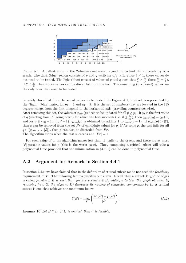
APPENDIX A. COMPUTING CRITICAL SUBSETS 101
q
p
1 2 3 4 5 6 7 8 9 10 11
1
2
3
4
5
6
7
4/7 p/q
Directions where p/q is increasing
2/3 2/6 2/10
5/10
1/4 1/8
3/9 3/5
4/11
7/11
1/11 1/1 1/2 1/3 1/5 1/6 1/7 1/9 1/10
2/2 2/4 2/5 2/7 2/8 2/9 2/11
3/3 3/4 3/6 3/7 3/8 3/10 3/11
4/8 4/9 4/10
5/9 5/11
6/10 6/11
Figure A.1: An illustration of the 2-dimensional search algorithm to find the vulnerability of agraph. The dark (blue) region consists of p and q verifying p/q > 1. Since θ ≤ 1, those values donot need to be tested. The light (blue) consist of values of p and q such that p
q > p0
q0(here p0
q0= 4
7).If θ < p0
q0, then, those values can be discarded from the test. The remaining (uncolored) values are
the only ones that need to be tested.
be safely discarded from the set of values to be tested. In Figure A.1, that set is represented bythe “light” (blue) region for p0 = 4 and q0 = 7. It is the set of numbers that are located in the 135degrees range, from the first diagonal to the horizontal axis (traveling counterclockwise).After removing this set, the values of qmin(p) need to be updated for all p ≥ p0. If q0 is the first valueof q (starting from |E| going down) for which the test succeeds (i.e. θ ≤ p0
q0), then qmin(p0) = q0 +1,
and for p ∈ p0 + 1, . . . ,V − 1, qmin(p) is obtained by adding 1 to qmin(p − 1). If qmin(p) > |E|,then p can be removed from the set Pr of candidate values for p. If for some p, the test fails for allq ∈ qmin, . . . , |E|, then p can also be discarded from Pr.The algorithm stops when the test succeeds and |Pr| = 1.
For each value of p, the algorithm makes less than |E| calls to the oracle, and there are at most|V| possible values for p (this is the worst case). Thus, computing a critical subset will take apolynomial time provided that the minimization in (4.191) can be done in polynomial time.
A.2 Argument for Remark in Section 4.4.1
In section 4.4.1, we have claimed that in the definition of critical subset we do not need the feasibilityrequirement of E. The following lemma justifies our claim. Recall that a subset E ⊆ E of edgesis called feasible if E is such that, for every edge e ∈ E, adding e to GE (the graph obtained byremoving from G, the edges in E) decreases its number of connected components by 1.. A criticalsubset is one that achieves the maximum below
θ(E) = maxE
(M(E)− µ(E)
|E|
). (A.2)
Lemma 10 Let E ⊆ E. If E is critical, then it is feasible.

APPENDIX A. COMPUTING CRITICAL SUBSETS 102
Table A.1: BinarySearch2D algorithm to compute θ and a critical subset. Algorithm Cunningham-Min is discussed in section 4.6.2. Method update method is presented in Table A.2.
BinarySearch2DInput: connected graph G = (V, E), V = n, E = m
Output:θ, E ⊆ E critical
1 begin2 Pr = 1,2,...,n-13 qmin = 1,2,...,n-14 while |Pr|>05 p <-- random(Pr)6 for q=m downto qmin(p)7 (E,minpq) = CunninghamMin((p/q)*1,G)8 if n-1 <= minpq then9 (Pr,qmin) = update(Pr,p,q)10 goto 411 end //if12 end //for13 Pr = Pr-p14 end //while15 return E, minpq16 end // begin
Table A.2: Pseudocode of the Update method used in the BinarySearch2D algorithm.UpdateInput: Pr, p ∈ Pr, q ∈ qmin, |E|Output: new Pr, qmin
1 begin2 qmin(p) = q+13 for j=p+1 to |n|-14 qmin(j) = qmin(j-1)+15 if qmin(j)>m6 Pr = Pr - j7 end //if8 end //for9 return Pr, qmin10 end //begin
APPENDIX A. COMPUTING CRITICAL SUBSETS 103
Proof: Let E be critical and not feasible. From Lemma 3, we have that M(E) = minT (|E ∩ T |) =Q(GE) − 1, where Q(GE) is the number of connected components of the graph GE obtained byremoving from G the edges in E. Now since E is not feasible, there exists an edge e ∈ E suchthat adding e to GE does not decrease its number of connected components. In other words,Q(GE) = Q(G
E\e), and as a consequence M(E) = M(E\e). This implies that
M(E\e)− µ(E\e)|E\e| − 1
=M(E)− (µ(E)− µ(e))
|E| − 1=M(E)− µ(E) + µ(e)
|E| − 1. (A.3)
This is strictly larger than M(E)|E| (the denominator has strictly decreased and the numerator has
increased), which means that E\e is strictly more critical than E. This contradicts the hypothesisthat E is critical.

104
Appendix B
Experimental Study
In chapters 2-4 of this thesis we have predicted the actions of both a rational attacker anda rational defender by analyzing the Nash equilibria for three communication scenarios. In thissection, our goal is to design an experimental study in order to generate real-life (laboratory) dataagainst which our theoretical predictions will be tested. In our experiments, we will only considerthe spanning tree game described in section 4.4.1. In that game, a defender is choosing a spanningtree of a graph to connect all nodes, while an attacker is targeting one link of the graph in orderto break the tree.
B.1 Motivations
Edges-connectivity has been widely considered as the vulnerability metric for graphs. The edge-connectivity of a connected graph is the minimum number of edges that need to be removed inorder to disconnect the graph; the corresponding set of edges is called a minimum cutset. In figureB.1, the minimum cutset of the graph corresponds to edges 1 and 4, giving a vulnerability (oredge-connectivity) of 2. The bold lines show an example of spanning tree of the network. Giventhis vulnerability metric, common sense might suggest that in the spanning tree game the attacker
1
2
7
5
3 4 6
Figure B.1: Example of network graph. The bold lines show one way to connect all nodes in thegraph without loop.

APPENDIX B. EXPERIMENTAL STUDY 105
will target edges of the minimum cutset to increase her chances of cutting the chosen spanningtree. This is so because the minimum cutset contains at least one link of each tree and it is theminimum set of links with this property.
In section 4.4.1, we have defined a critical subset of edges of a graph to be a subset that maximizesthe minimum fraction of edges it has in common with any tree (minT (|T∩E|)
|E| ). We have proposedthis maximum value as the vulnerability metric of the graph. We have also shown that a minimumcutset of a graph is not necessarily critical and that a rational attacker will target edges on acritical subset (not a minimal cutset) and attack them with the same probability. Furthermore,we have shown that if the attacker incurs a cost of attacking the links, she will target a subsetthat maximizes (minT (|T∩E|)
|E| − µ(E)|E| ) which is the minimum fraction of edges it has n common with
any tree minus the average cost of attack of the subset. The attacker does not launch an attackif this difference is negative. Otherwise, she attack links in a maximizing subset with the sameprobability.
The goal of this experimental study is to test those predictions with subjects in a laboratorysetting. More precisely, we would like to assess the minimum cutset assumption (game 1), thecritical subset attack (game 2), the uniformity of attack (all games), and the dependency on theattack cost (games 3,4,5).
The games considered in our experiments, are played by a user (the subject) and a machine (thedefender). The role of the user is to attack one link of the network in order to break the spanning treeselected by the machine. The machine chooses a spanning according to the distribution predictedby the Nash equilibria analysis.
In each game, the subject will be asked to choose one link to attack and win up to 70 tokens.The number 70 is just chosen for convenience reasons. To simulate mixed strategies, the subjectis given the choice to bet all tokens on one link, or to distribute the tokens on a selected subset oflinks and indicate how many tokens to bet on each link. When there is no cost of attack, the totalnumber of tokens bet on links belonging to the selected spanning tree is won by the attacker. Ifthe cost of attacking any link is positive, the reward of the users is given by the total number oftokens bet on links belonging to the selected spanning tree minus the cost of attacking such links.
The questions that we would like to answer with these experiments are the following:
• Which set of links will be attacked and how many tokens are bet by the subjects? By dividingthe number of tokens bet on each link by the total number of tokens, we get a probabilitydistribution that can be interpreted as the mixed strategy of the player.
• Do subject follow the “common sense” attack that targets a minimum cutset of the graph?
• Do subjects target links uniformly?
• How do subjects behave when the cost of attack is larger/equal/smaller than the maximumexpected gain?

APPENDIX B. EXPERIMENTAL STUDY 106
1
2
7
5 3
4
6
8
9
10 13
14
12
11
(a) Topology of the network used in experi-ment 1. The network contains one minimumcutset (6, 8) which also is a critical subset.
1
2
7
5 3
4
6
8
9
10
13
12 11
(b) Topology of the network used in experi-ment 1. The network contains one minimumcutset (6, 8). This minimum cutset is how-ever not a critical subset.
Figure B.2: Networks considered in experiments 1 (B.2(a)) and 2 (B.2(b)).
To answer these questions, we collect data by letting the subjects play the following 5 games. Inthe first two game, there is no cost of attack. In the last three, the attacker (subject) incurs apositive cost when attacking a link.
B.2 Game 1
The graph considered in this game is depicted in figure B.2(a). It contains one minimum cutset(6, 8, the only one) which also is a critical subset. There are three other critical subsets: the setof all links, the set 1, 2, 3, 4, 5, 6, 7, 8, and the set 6, 8, 9, 10, 11, 12, 13, 14. In this experiment,we would like to test the minimum cut attack prediction, which is the optimal strategy in this casebecause the minimum cutset is critical. Also, because of the symmetry of the graph, we expectsubjects to uniformly target edges in the minimum cutset. The predicted (average) attack rewardis 35 tokens which can be achieved by betting 35 tokens for each links in the minimum cutset.
B.3 Game 2
Game 2 is played on the graph shown in figure B.2(b). As before, it contains one minimum cutset(6, 8). However, unlike this previous case, the minimum cutset in this figure is not critical.The graph contains one critical subset that corresponds to edges 6, 8, 9, 10, 11, 12, 13. The NEanalysis predicts that a rational attacker will only target edges in the critical subset and will attackthem with the same probability. The predicted (average) attack reward is 40 tokens which canbe achieved by betting 10 tokens on each link of the critical subset. In this experiment, we testwhether users plays according to the NE prediction.

APPENDIX B. EXPERIMENTAL STUDY 107
B.4 Games 3,4,5
The next games are played on the graph in B.2(b). In game 3, we assume that the attackerincurs a cost of µ = [22 39 27 5 17 3 22 19 42 35 21 38 6 17] tokens on the links. Withthis cost, the predicted average attack reward is equal to 24 token and the maximizing sub-set corresponds to the minimum cutset 6, 8. With this reward, a rational attacker shouldalways attack uniformly the edges 6 and 8. Game 4 is played with an attack cost equal toµ = [5 63 5 31 58 28 43 58 63 66 14 19 63 42]. The corresponding maximum average attackreward is equal to −1 and is achieved at subset 1, 2, 3. In this case, the NE analysis suggeststhat a rational player will opt to not attack the network. In the last game (game 5), the costincurred by the attacker is equal to µ = [10 61 30 29 68 53 69 17 7 27 36 40 69 35]. It gives amaximum average reward of zero. Two subsets achieve this reward: the minimum cutset 6, 8 andthe subset 6, 8, 9, 10, 11. This is a case where attacking and not attacking give the same rewardto the attacker.
In these three experiments, we are interesting in determining how the introduction of the costof attack will influence the subjects’ attack strategies. In the first experiment, the attack costs arenot too high and there is an strategy that gives positive reward. In the second one, no strategycan give positive reward and subjects are expected to not play. In the last game, playing and notplaying give the same payoff to the subjects.