A Fuzzy Logic Controller for a Hydrostatic Transmission ...
50
A Fuzzy Logic Controller for a Hydrostatic Transmission for an Electric Hybrid Bus in Bogota Presented as a partial requirement for a master degree in mechanical engineering by Jorge Andres Leon Quiroga Advised by Andres Leonardo Gonzalez Mancera, PhD, main advisor Universidad de los Andes Jose Manuel Garcia, PhD, co – advisor Purdue University Universidad de los Andes Faculty of Engineering Department of Mechanical Engineering Bogota, Colombia 2016
Transcript of A Fuzzy Logic Controller for a Hydrostatic Transmission ...
A Fuzzy Logic Controller for a Hydrostatic Transmission for an Electric Hybrid Bus in
Bogota
Presented as a partial requirement for a master degree in mechanical engineering by
Jorge Andres Leon Quiroga
Advised by
Andres Leonardo Gonzalez Mancera, PhD, main advisor
Universidad de los Andes
Jose Manuel Garcia, PhD, co – advisor
Purdue University
Universidad de los Andes
Faculty of Engineering
Department of Mechanical Engineering
Bogota, Colombia
2016

Page 2 of 50
Agradecimientos.
Quiero agradecer a mis padres por su apoyo incondicional y porque desde siempre han sido
los mejores maestros que he tenido. Quiero agradecer también a mis hermanas porque
siempre han sido y serán las mejores amigas que tendré. Quiero agradecer también a todas
las personas que me han acompañado durante mi camino y que siempre han estado dispuestos
a apoyarme. En especial quiero agradecer a María Paula Mejía por su invaluable apoyo y
compañía.

Page 3 of 50
1. Content
1. Content ............................................................................................................................ 3
2. Abstract ........................................................................................................................... 4
3. Introduction ..................................................................................................................... 4
4. Objectives ........................................................................................................................ 6
Main objective .................................................................................................................... 6
Specific objectives .............................................................................................................. 6
5. Vehicle model ................................................................................................................. 7
5.1 Powertrain architecture ................................................................................................. 7
5.1.1 Hydrostatic transmission ........................................................................................ 8
5.1.2 Regenerative braking energy system...................................................................... 9
5.1.3 Accumulator discharge ........................................................................................... 9
5.2 Dynamic model ........................................................................................................... 10
5.3 Coupled model ............................................................................................................ 12
6. Case of study ................................................................................................................. 15
7. Control strategy ............................................................................................................. 20
7.1 Study of the system efficiency .................................................................................... 20
7.2 Fuzzy logic control ..................................................................................................... 23
7.3 Driver response model ................................................................................................ 24
7.4 Hydraulic system control ............................................................................................ 29
8. Results ........................................................................................................................... 35
8.1 Driver response model ................................................................................................ 35
8.2 Hydraulic transmission control ................................................................................... 37
8.3 Energetic analysis ....................................................................................................... 39
9. Conclusions ................................................................................................................... 41
10. Future work................................................................................................................ 43
11. Bibliography .............................................................................................................. 44
Appendix .............................................................................................................................. 46

Page 4 of 50
2. Abstract The control strategy in a hydraulic hybrid vehicle is very important for taking advantage of
its full potential. In a hydraulic hybrid vehicle, the hydrostatic transmission can be controlled
in order to optimize the entire system. A hydrostatic transmission is composed basically of a
hydraulic motor and a hydraulic pump. For an electric hybrid vehicle an electric motor is the
prime mover. In this study the control variables are the displacements of the hydraulic devices
and the objective is to optimize the system efficiency. All possible combinations of
displacements were tested through simulation and the most efficient combination was
recorded. Around 9% of the energy can be saved using the most efficient configuration of
the hydrostatic transmission. Fuzzy logic theory was used to simulate the driver input and
proposed as a control strategy for the hydrostatic transmission.
3. Introduction
The continuous diminishing of oil reserves and the increasing demand of energy is a
worldwide problem. Nowadays there are many alternatives for supplying energy such as
renewable energy, nuclear energy, biofuel energy, etc. Another option for reducing the
impact of gas emissions is improving the efficiency of the systems and devices that are
already in use. Any improvement in the efficiency of devices can be significant and can have
a global impact. In 2013 in the United States the transportation sector consumed 69% of all
petroleum. So, improving the efficiency of the transportation systems can have a huge impact
in the global energy consumption [1].
Due to recent concern about reducing emissions in traditional combustion engine vehicles,
electric vehicles have been considered in the last years as an alternative for replacing the
traditional vehicles. Electric vehicles use an electric motor as the prime mover and flywheels,
fuel cells, ultracapacitors and batteries as energy sources. The advantages of electric vehicles
over internal combustion engine vehicles are the high efficiency, smooth and quiet operation,
no emissions and independence of petroleum based fuels [2].
Powertrain hybridization trough hydraulic transmission is one of the available options for
improving efficiency in electric car [3]. On-road hybrid vehicle market is dominated by
electric hybrids, however hydraulic hybrids have many benefits which make them a
competing technology. It has been demonstrated that hydraulic hybrid transmissions increase
29% the fuel efficiency over the most efficient electric hybrid and 47% over an identical
non-hybrid bus [4]. Moreover, the lifecycle cost of the hydraulic hybrid is 24% less than a
conventional diesel bus and 36% less than an electric hybrid bus. Hydraulic hybrids use
hydraulic accumulators as energy storage devices. Accumulators have a longer lifecycle than
batteries and the batteries need to be replaced one or more times over their lifetime depending
on application [5].

Page 5 of 50
Hydraulic hybrid transmissions can be grouped into three main categories: parallel hybrids,
series hybrids and hybrid power split transmissions. Each of them have benefits and
drawbacks. These systems have been installed and studied in vehicles such as delivery trucks
[6], refuse collection vehicles [7] and pickup trucks [3] with satisfactory results. The focus
of this work is on series hybrids because of the simplicity of the system, ease of installation
compared with other hydraulic systems, and because of its stiff nature that enables rapid
changes in system pressure which is very important for satisfying the driver demands [8].
The control strategy of the system is very important in order to take advantage of its full
potential. Some of the controllers developed until now has been designed for internal
combustion engines and hybrid electric vehicles [9] [10]. Load leveling is a methodology in
which the internal combustion engine is forced to operate around its most efficient point.
This methodology has demonstrated great potential. However, in diesel engines the most
efficient operating point is near to the peak torque curve, which is the region of maximum
fuel consumption [11].
Fuzzy logic control is a convenient way to control hybrid vehicles. This has been
demonstrated in previous research at Oakland University [12] [13] and Ohio State University
[14] [15]. Some studies have focused on hybrid electric vehicles and their principal concern
has been the power management strategy. That is the magnitude and rate at which the power
needed by the car is delivered to the wheels [11]. Another study is focused on optimizing all
components of the system in order to obtain the most efficient combination of variables [16].
Also, dynamic programming has been used to control hybrid hydraulic vehicles with good
results [17]. An instantaneous optimization is made in dynamic programming. This method
allows to compare in a fair way many options of hydrostatic transmissions [18].
In this work, a fuzzy logic control is proposed as a control strategy for a hydrostatic
transmission in an electric bus for the Integrated Public System of Transportation (SITP) in
Bogota, Colombia. A numerical model was developed in order to choose the elements of the
system. These elements were selected in order to provide the vehicle requirements for a
typical urban driving cycle. After that, a fuzzy logic control was used to model the human
response and it was proposed as a control strategy for the vehicle.

Page 6 of 50
4. Objectives
Main objective
Evaluate the performance of a fuzzy logic controller for a hydrostatic transmission for an
electric hybrid vehicle in Bogota, Colombia.
Specific objectives
Study and specify the operation conditions, requirements and constraints of the
problem.
Design the hydrostatic transmission.
Design the control strategy.
Evaluate the performance of the system and the control strategy through simulation.
Page 7 of 50
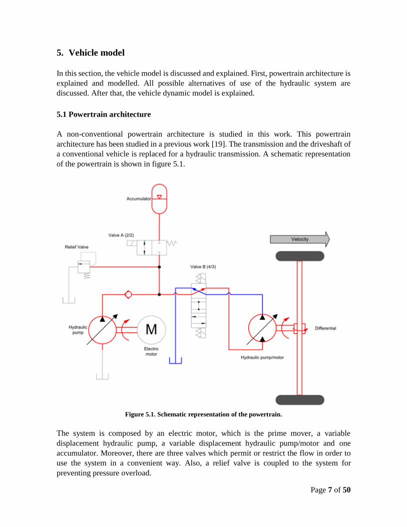
5. Vehicle model
In this section, the vehicle model is discussed and explained. First, powertrain architecture is
explained and modelled. All possible alternatives of use of the hydraulic system are
discussed. After that, the vehicle dynamic model is explained.
5.1 Powertrain architecture
A non-conventional powertrain architecture is studied in this work. This powertrain
architecture has been studied in a previous work [19]. The transmission and the driveshaft of
a conventional vehicle is replaced for a hydraulic transmission. A schematic representation
of the powertrain is shown in figure 5.1.
Figure 5.1. Schematic representation of the powertrain.
The system is composed by an electric motor, which is the prime mover, a variable
displacement hydraulic pump, a variable displacement hydraulic pump/motor and one
accumulator. Moreover, there are three valves which permit or restrict the flow in order to
use the system in a convenient way. Also, a relief valve is coupled to the system for
preventing pressure overload.

Page 8 of 50
This system can work in three ways: as a hydrostatic transmission, as a recovery braking
energy system and as a system propelled by the energy stored in the accumulator. Each of
these operation modes are explained next.
5.1.1 Hydrostatic transmission
The hydraulic system can be used as a hydrostatic transmission in order to transmit power
from the electric motor to the wheels. The electric motor is the prime mover and the pump
moves the fluid from the reservoir to the hydraulic pump/motor which in this case is working
as a motor. For this process valve A is closed while valve B is in the higher position (see
figure 5.1). The flow through the hydraulic motor generates the power to move the vehicle.
Equations 5.1 to 5.3 are the equilibrium equations for each component of the hydrostatic
transmission.
Electric motor
𝐼𝐸𝑀�̇�𝐸𝑀 = 𝑇𝐸𝑀 − 𝑇𝑝 (5.1)
Hydraulic pump
𝐼𝑝�̇�𝑝 = 𝑇𝑝 − 𝑀𝑝 (5.2)
Hydraulic motor
𝐼𝑚�̇�𝑚 = 𝑀𝑚 − 𝑇𝑚 (5.3)
Where 𝐼 is the mass inertia of the component, 𝑇 is the torque delivered by the component, �̇�
is the angular acceleration and 𝑀 is the hydraulic torque. The subscripts 𝐸𝑀, 𝑝 and 𝑚
indicate electric motor, hydraulic pump and hydraulic motor respectively. Hydraulic torque
in the pump and the motor are calculated with equations 5.4 and 5.5.
𝑀𝑃 = Δ𝑃𝐷𝑝 𝜂𝑚,𝑝⁄ (5.4)
𝑀𝑚 = Δ𝑃𝐷𝑚𝜂𝑚,𝑚 (5.5)
Where Δ𝑃 is the pressure drop in the system, 𝐷 is the displacement and 𝜂𝑚 is the mechanical
efficiency. Again, subscripts 𝑝 and 𝑚 indicate hydraulic pump and hydraulic motor
respectively. Moreover, the flow rate in the pump and the motor is given by equations 5.6
and 5.7 respectively.
𝑄𝑝 = 𝜔𝑝𝐷𝑝𝜂𝑣,𝑝 (5.6)
𝑄𝑚 = 𝜔𝑚𝐷𝑚 𝜂𝑣,𝑚⁄ (5.7)
Where 𝜔 is the angular velocity and 𝜂𝑣 is the volumetric efficiency.
Page 9 of 50
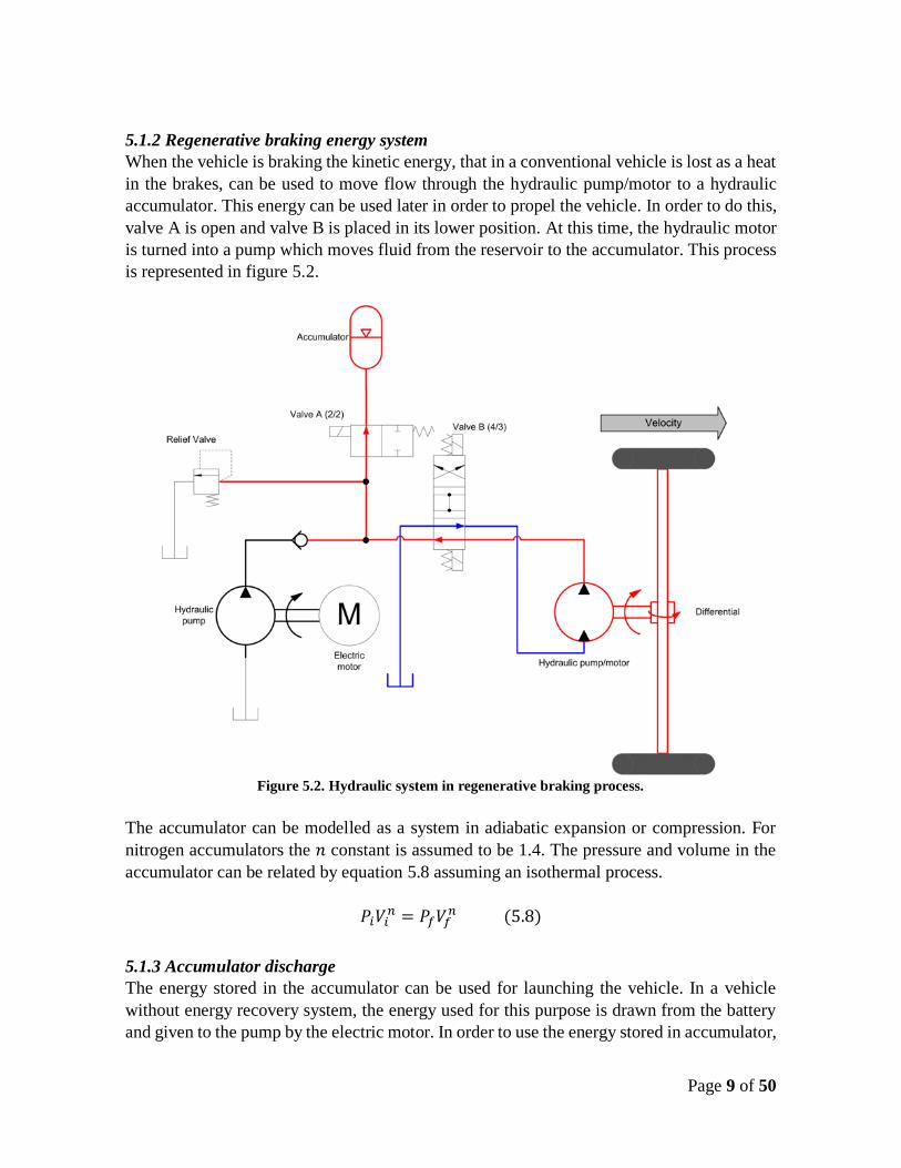
5.1.2 Regenerative braking energy system
When the vehicle is braking the kinetic energy, that in a conventional vehicle is lost as a heat
in the brakes, can be used to move flow through the hydraulic pump/motor to a hydraulic
accumulator. This energy can be used later in order to propel the vehicle. In order to do this,
valve A is open and valve B is placed in its lower position. At this time, the hydraulic motor
is turned into a pump which moves fluid from the reservoir to the accumulator. This process
is represented in figure 5.2.
Figure 5.2. Hydraulic system in regenerative braking process.
The accumulator can be modelled as a system in adiabatic expansion or compression. For
nitrogen accumulators the 𝑛 constant is assumed to be 1.4. The pressure and volume in the
accumulator can be related by equation 5.8 assuming an isothermal process.
𝑃𝑖𝑉𝑖𝑛 = 𝑃𝑓𝑉𝑓
𝑛 (5.8)
5.1.3 Accumulator discharge
The energy stored in the accumulator can be used for launching the vehicle. In a vehicle
without energy recovery system, the energy used for this purpose is drawn from the battery
and given to the pump by the electric motor. In order to use the energy stored in accumulator,
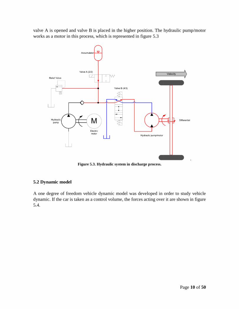
Page 10 of 50
valve A is opened and valve B is placed in the higher position. The hydraulic pump/motor
works as a motor in this process, which is represented in figure 5.3
. Figure 5.3. Hydraulic system in discharge process.
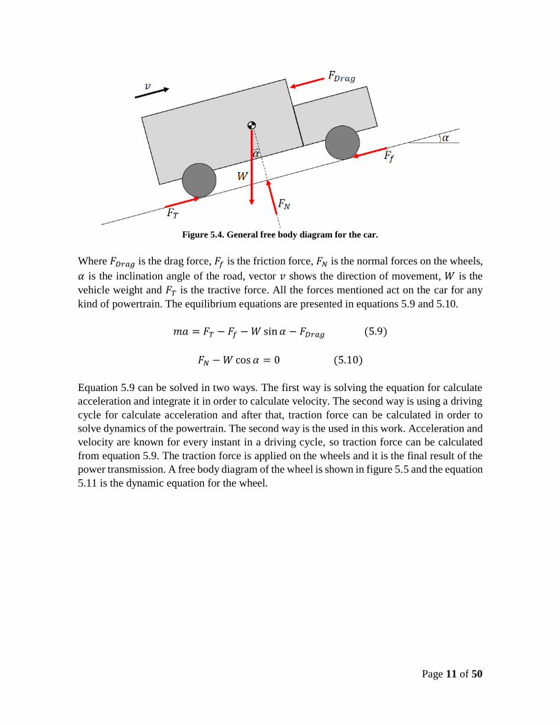
5.2 Dynamic model
A one degree of freedom vehicle dynamic model was developed in order to study vehicle
dynamic. If the car is taken as a control volume, the forces acting over it are shown in figure
5.4.
Page 11 of 50
Figure 5.4. General free body diagram for the car.
Where 𝐹𝐷𝑟𝑎𝑔 is the drag force, 𝐹𝑓 is the friction force, 𝐹𝑁 is the normal forces on the wheels,
𝛼 is the inclination angle of the road, vector 𝑣 shows the direction of movement, 𝑊 is the
vehicle weight and 𝐹𝑇 is the tractive force. All the forces mentioned act on the car for any
kind of powertrain. The equilibrium equations are presented in equations 5.9 and 5.10.
𝑚𝑎 = 𝐹𝑇 − 𝐹𝑓 − 𝑊 sin 𝛼 − 𝐹𝐷𝑟𝑎𝑔 (5.9)
𝐹𝑁 − 𝑊 cos 𝛼 = 0 (5.10)
Equation 5.9 can be solved in two ways. The first way is solving the equation for calculate
acceleration and integrate it in order to calculate velocity. The second way is using a driving
cycle for calculate acceleration and after that, traction force can be calculated in order to
solve dynamics of the powertrain. The second way is the used in this work. Acceleration and
velocity are known for every instant in a driving cycle, so traction force can be calculated
from equation 5.9. The traction force is applied on the wheels and it is the final result of the
power transmission. A free body diagram of the wheel is shown in figure 5.5 and the equation
5.11 is the dynamic equation for the wheel.

Page 12 of 50
Figure 5.5. Free body diagram for the wheel.
𝐼𝑤�̇�𝑤 = 𝑇𝑇 − 𝐹𝑇𝑅𝑤 (5.11)
Where 𝐼𝑤 is the mass inertia of the wheel, �̇�𝑤 is the angular acceleration, 𝑇𝑇 is the traction
torque and 𝑅𝑤 is the wheel radius. With equations 5.9 and 5.11 and the driving cycle, the
acceleration, velocity, tractive force and tractive torque can be calculated.
The equations presented here are the same for a common commercial vehicle with an internal
combustion engine and mechanical powertrain. The principal differences between a common
vehicle and the one studied in this work is in the powertrain. In a common commercial
vehicle, the powertrain is composed by mechanical gears that transmit the power from the
engine to the wheels in a convenient manner, while in a hybrid hydraulic vehicle the power
transmission is through the components of the hydrostatic transmission. The relationships
between displacements of the hydraulic components allow to transmit power as the
mechanical transmission.
5.3 Coupled model
Dynamic and hydraulic models must be solved in a coupled way. The equations that model
the entire system are presented again here:
Electric motor
𝐼𝐸𝑀�̇�𝐸𝑀 = 𝑇𝐸𝑀 − 𝑇𝑝 (5.1)
Hydraulic pump
𝐼𝑝�̇�𝑝 = 𝑇𝑝 − 𝑀𝑝 (5.2)
Hydraulic motor
𝐼𝑚�̇�𝑚 = 𝑀𝑚 − 𝑇𝑚 (5.3)

Page 13 of 50
Hydraulic torque in the pump
𝑀𝑃 = Δ𝑃𝐷𝑝 𝜂𝑚,𝑝⁄ (5.4)
Hydraulic torque in the hydraulic motor
𝑀𝑚 = Δ𝑃𝐷𝑚𝜂𝑚,𝑚 (5.5)
Flow rate in the pump
𝑄𝑝 = 𝜔𝑝𝐷𝑝𝜂𝑣,𝑝 (5.6)
Flow rate in the hydraulic motor
𝑄𝑚 = 𝜔𝑚𝐷𝑚 𝜂𝑣,𝑚⁄ (5.7)
Dynamic equation for the vehicle
𝑚𝑎 = 𝐹𝑇 − 𝐹𝑓 − 𝑊 sin 𝛼 − 𝐹𝐷𝑟𝑎𝑔 (5.9)
Dynamic equation for the wheel
𝐼𝑤�̇�𝑤 = 𝑇𝑇 − 𝐹𝑇𝑅𝑤 (5.11)
In order to solve these equations, some assumptions must be taken into account:
1. Flow rate out of the pump is the same entering to the hydraulic motor, so 𝑄𝑝 = 𝑄𝑚
2. Pressure drop in the pump and the hydraulic motor is the same.
3. There is no slip in the tires.
With the first assumption (𝑄𝑝 = 𝑄𝑚), a relationship between velocity in the hydraulic motor
and velocity in the pump can be made.
𝜔𝑝 = 𝜔𝑚
𝐷𝑚
𝐷𝑝
1
𝑛𝑣,𝑚𝑛𝑣,𝑝 (5.12)
With the third assumption a relationship between car velocity and wheel velocity can be
made. A similar relationship can be made for acceleration.
𝜔𝑤 = 𝑉 𝑅𝑤⁄ (5.13)
�̇�𝑤 = 𝑎 𝑅𝑤⁄ (5.14)
With equations 5.13 and 5.14, motor angular velocity and angular acceleration can be
calculated.
𝜔𝑚 = 𝜔𝑤𝑁𝑑𝑖𝑓 (5.15)
�̇�𝑚 = �̇�𝑤𝑁𝑑𝑖𝑓 (5.16)

Page 14 of 50
With a similar equation, torque in the hydraulic motor can be calculated as a function of the
traction torque in the wheel.
𝑇𝑚 = 𝑇𝑇 𝑁𝑑𝑖𝑓⁄ (5.17)
Pump angular acceleration is given by equation 5.18: �̇�𝑝 = 𝑑𝜔𝑝 𝑑𝑡⁄ (5.18)
Between the electric motor and the hydraulic pump, it is necessary to have a gear. The
relationship between hydraulic pump velocity and electric motor velocity is given by
equation 5.19. In a similar way, with equation 5.20 the electric motor angular acceleration
can be calculated.
𝜔𝐸𝑀 = 𝜔𝑝𝑁𝑑𝑖𝑓,𝑝 (5.19)
�̇�𝐸𝑀 = �̇�𝑝𝑁𝑑𝑖𝑓,𝑝 (5.20)
The method used for solving the system of equations is described next.
1. From the driving cycle, acceleration and velocity are determined.
2. From equation 5.9 tractive force is calculated.
3. From equations 5.13 to 5.16 angular velocity and acceleration of the wheels and the
hydraulic motor are determined.
4. Tractive torque in the wheels are determined by equation 5.11.
5. Torque in the hydraulic motor can be solved from equation 5.17.
6. From equation 5.3, hydraulic torque (𝑀𝑚) in the hydraulic motor is calculated.
7. Pressure drop in the system is calculated from equation 5.5.
8. From equation 5.4, hydraulic torque (𝑀𝑝) in the hydraulic pump is calculated.
9. Pump angular velocity is calculated from equation 5.12.
10. Pump angular acceleration is calculated with a discretized approximation of equation
5.18. �̇�𝑝 = (𝜔𝑖 − 𝜔𝑖−1) Δ𝑡⁄
11. From equation 5.2, torque in the hydraulic pump is calculated.
12. Electric motor angular acceleration is calculated with equation 5.20.
13. From equation 5.1, torque in the electric motor is determined.
The method described is used to select the hydraulic components of the hydrostatic
transmission. With this method it is possible to determine the energy consumption of the
hydrostatic transmission for a determined driving cycle. Moreover, it is possible to determine
the influence of some variables related with the hydraulic components as their mass inertia
and displacements.

Page 15 of 50
6. Case of study
The case of study of this work is a commercial passenger bus Chevrolet NKR Reward Euro
IV which is a typical bus of the Integrated Public System of Transportation (SITP) in Bogota.
This vehicle uses an internal combustion engine as a prime mover. An example of this bus is
presented in figure 6.1.
Figure 6.1. Urban route of SITP
The principal characteristics of this bus are described in table 6.1.
Table 6.1 Vehicle specifications.
The driving cycles are widely used for estimation of fuel consumption and other performance
characteristics in vehicles. As a reference, an urban driving cycle of an articulated bus of
Transmilenio was used [20]. The driving cycle is shown in figure 6.2.

Page 16 of 50
Figure 6.2. Urban driving cycle [20].
The equations written in chapter 5 were used to select the components of the system. First,
hydraulic motor was selected in order to satisfy the torque and angular velocity requirements
of the driving cycle presented in figure 6.2. With the driving cycle it is possible to have the
velocity and acceleration, with equations 5.9 and 5.11 the tractive force and the tractive
torque can be calculated. The hydraulic motor must be able to satisfy this requirement of
tractive torque and angular velocity because it is directly attached to the wheels through the
differential. Many hydraulic motors were compared. The comparison between limits of the
hydraulic motors and requirements of the vehicle for the driving cycle chosen as a reference
are presented in figure 6.3.
Figure 6.3. Comparison of hydraulic motors.

Page 17 of 50
From the figure it is possible to determine that the motor of 165 cc/rev is capable of satisfying
the requirements. The principal characteristics of this hydraulic motor are described in table
6.2.
Table 6.2. Hydraulic motor specifications.
In a similar way, requirements of the vehicle were compared with capabilities of many
hydraulic pumps. In figure 6.4, this comparison is shown for the pump chosen.
Figure 6.4. Comparison of hydraulic pump limits.
From this figure it is possible to see that the pump is able to satisfy the requirements of the
vehicle even when it works with either its maximum or minimum displacement. So, this
pump can be used as a variable displacement pump. Using the pump as a variable
displacement device, allows to have a continuous variable transmission, which can be used
in order to adjust the torque and angular velocity in the prime mover for doing it to work
more efficiently. The principal characteristics of the hydraulic pump are described in table
6.3.

Page 18 of 50
Table 6.3. Hydraulic pump specifications.
Now, an electric motor must be selected in order to be the prime mover of the system. The
motor selected was a REMY HVH 250, which is widely used for electric cars. The principal
characteristics of this motor are shown in table 6.4.
Table 6.4. Electric motor specifications.
This electric motor is capable of satisfying the requirements of the system for the driving
cycle chosen as a reference (figure 6.2). A comparison between requirements of the system
and motor limits are shown in figures 6.5 and 6.6. These figures show the requirements when
the pump is working with either its maximum or minimum displacements.
Figure 6.5. Comparison between system requirements and motor torque limit.

Page 19 of 50
Figure 6.5. Comparison between system requirements and motor power limit.
The devices selected are capable of satisfying the requirements of the vehicle for a typical
driving cycle. Moreover, because of the possibility of a continuous variable transmission, the
system can be optimized at every time in order to rise the efficiency and diminish the spent
of energy.

Page 20 of 50
7. Control strategy
The control strategy of the system is very important for taking advantage of its full potential.
It is important to optimize all the system and not a particular device of the system. Also, it is
important that the control system has as an input signal something that can be measured easily
and related with the driver intention as the percentage of compression of the pedals. In a
conventional internal combustion engine vehicle, the driver adjusts the torque of the motor
with the pedals in order to reach a desired velocity and acceleration. The objective of the
control system is to optimize the system every time, whatever can be the driver desire. In
other words, the only concern of the driver must be maintaining the desired velocity and the
control system must optimize the entire system.
7.1 Study of the system efficiency
The final purpose of any powertrain is to transfer the power from the engine to the wheels
and move the vehicle. The power delivered by the motor is reflected in the vehicle velocity
and in the tractive torque at the wheels. For any kind of powertrain, if the driver wants to
move to any specific velocity, the car needs a specific tractive torque at the wheels. For this
reason, the powertrain performance is analyzed in terms of tractive torque and vehicle
velocity. There are many possible configurations of the hydraulic system that allow the
vehicle to move with those tractive torque and velocity, but there is one optimal
configuration.
An instantaneous quasi-static optimization is performed for a discrete mesh of tractive torque
versus velocity. At each combination of tractive torque and velocity the efficiency of the
entire powertrain is optimized. For each combination of tractive torque and velocity, all the
possible combinations of hydraulic motor displacement and hydraulic pump displacement
are tested. For a specific combination of hydraulic motor and hydraulic pump displacement,
hydrostatic transmission variables such as pressure system, hydraulic motor and hydraulic
pump velocities, flow rate and efficiency are calculated and the constraints are verified. The
most efficient combination of displacements for every tractive torque and vehicle velocity is
recorded as well as all other variables associated with the hydrostatic transmission. The
process is described schematically in figure 7.1.

Page 21 of 50
Figure 7.1. Schematic representation of the process.
Optimal hydraulic motor displacement and hydraulic pump displacement are shown in
figures 7.2 and 7.3.

Page 22 of 50
Figure 7.2. Optimal hydraulic motor displacement.
Figure 7.3. Optimal hydraulic pump displacement.
From figure 7.2 it is possible to see that the hydraulic motor displacement is low for low
tractive torque and high for high tractive torque. Hydraulic pump displacement, on the other
hand, is almost the same for the most of possible combinations of tractive torque and velocity.
So, from these figures it is possible to conclude that a good hydraulic transmission can be

Page 23 of 50
composed of a variable displacement hydraulic motor and a fixed displacement hydraulic
pump.
The optimal total efficiency of the hydrostatic transmission is shown in figure 7.4. From this
figure it is possible to see that the hydraulic transmission can reach efficient values of 80%,
but the efficiency is low for low values of tractive torque. In this region of the figure the
efficiency is between 3% and 65%. An alternative for improving the efficiency can be the
use of a power split transmission, which can be activated for low torque values [3].
Figure 7.4. Optimal total efficiency of the hydrostatic transmission.
7.2 Fuzzy logic control
The objective of the control system is to try to maintain the hydraulic system as close as
possible of its most efficient point. This can be achieved using a convenient control strategy.
It has been demonstrated that fuzzy logic control could be applied to the design of electric
hybrid vehicles [21] [22] and hydrostatic transmissions [23].
Fuzzy logic control is able to handle with numerical data and with linguistic variables. For
example, the driver intention can be measured with the percentage of compression of the
pedals. If the acceleration pedal is compressed to 100%, the driver wants to accelerate as
much as the motor allow it. This case can be associated with the linguistic variable "High
acceleration". In this work, fuzzy logic was used to model the driver input and also it was
used as a control strategy for the hydrostatic transmission.

Page 24 of 50
7.3 Driver response model
In the real life the driver controls velocity and acceleration with braking and acceleration
pedals. If he wants to go faster, he pushes the accelerator. If he wants to go slower, he stops
depressing the accelerator if the desired deceleration is not so big, and begin to push the brake
pedal if he wants a bigger deceleration. So, the velocity and acceleration must be the inputs
to the driver model. The outputs must be the percentages of compression of the brake and
acceleration pedals.
The theoretical percentage of compression for both, brake and accelerator pedals, can be
calculated analytically. Traction force can be calculated from equation 9 for any value of
acceleration and vehicle velocity. The product of traction force and velocity is equal to the
power delivered to the vehicle. This power is a percentage of the power that the motor can
deliver. This percentage is directly related with the percentage of compression of the pedals.
If the driver wants all the power, he will push the accelerator in a 100%. So, the theoretical
percentage of compression is defined as the ratio between the product of traction force and
vehicle velocity and the power that the motor can delivered. This theoretical value can be
used in order to estimate the driver intention for any possible combination of acceleration
and vehicle velocity. A map of theoretical percentage of pedal compression is shown in figure
7.5. For instance, if the vehicle is going to 40 km/h and its acceleration is 0.6 𝑚/𝑠2, the
percentage of compression for the acceleration pedal must be equal or very close to 50 %.
Figure 7.5. Theoretical percentage of accelerator pedal.
In a similar way, there is a limit for the maximum braking force. This limit depends of many
factors such as slip ratio and temperature. In this work, as a first approach, a constant
coefficient of friction will be assumed [24]. Traction force can be calculated again from
equation 9 and compared with the maximum braking force. The theoretical percentage of

Page 25 of 50
compression is defined as the ratio between the traction force and the maximum braking
force. A map of theoretical percentage of compression of brake pedal is shown in figure 7.6.
In this figure there is a region in which the percentage of compression is zero. This is because
the rolling resistance and the drag force is enough to decelerate the vehicle.
Figure 7.6. Theoretical percentage of brake pedal.
With figures 7.5 and 7.6 it is possible to define the membership functions, fuzzy sets and
fuzzy rules. This must be related with linguistic variables associated with the information of
the figures. For example, when the acceleration is positive and very high and the velocity is
very low, the percentage of compression of the accelerator is very high. When the
acceleration is negative and very low and the velocity is very low, the percentage of
compression of the brake pedal is zero. The driver response model has three inputs: vehicle
velocity, vehicle acceleration and error. The error is calculated with equation 7.1.
𝑒𝑟𝑟𝑜𝑟 =𝑣𝑎𝑐𝑡𝑢𝑎𝑙 − 𝑣𝑟𝑒𝑓𝑒𝑟𝑒𝑛𝑐𝑒
𝑣𝑎𝑐𝑡𝑢𝑎𝑙 (7.1)
The membership functions for all the inputs are shown in figures 7.7, 7.8 and 7.9. The output
of the driver response model is the percentage of compression of the pedals. The membership
functions for the outputs are shown in figure 7.10.

Page 26 of 50
Figure 7.7. Membership functions for the vehicle acceleration.
Figure 7.8. Membership functions for the vehicle velocity.
Figure 7.9. Membership functions for the error.
Figure 7.10. Membership functions for the compression of the pedals.
Page 27 of 50
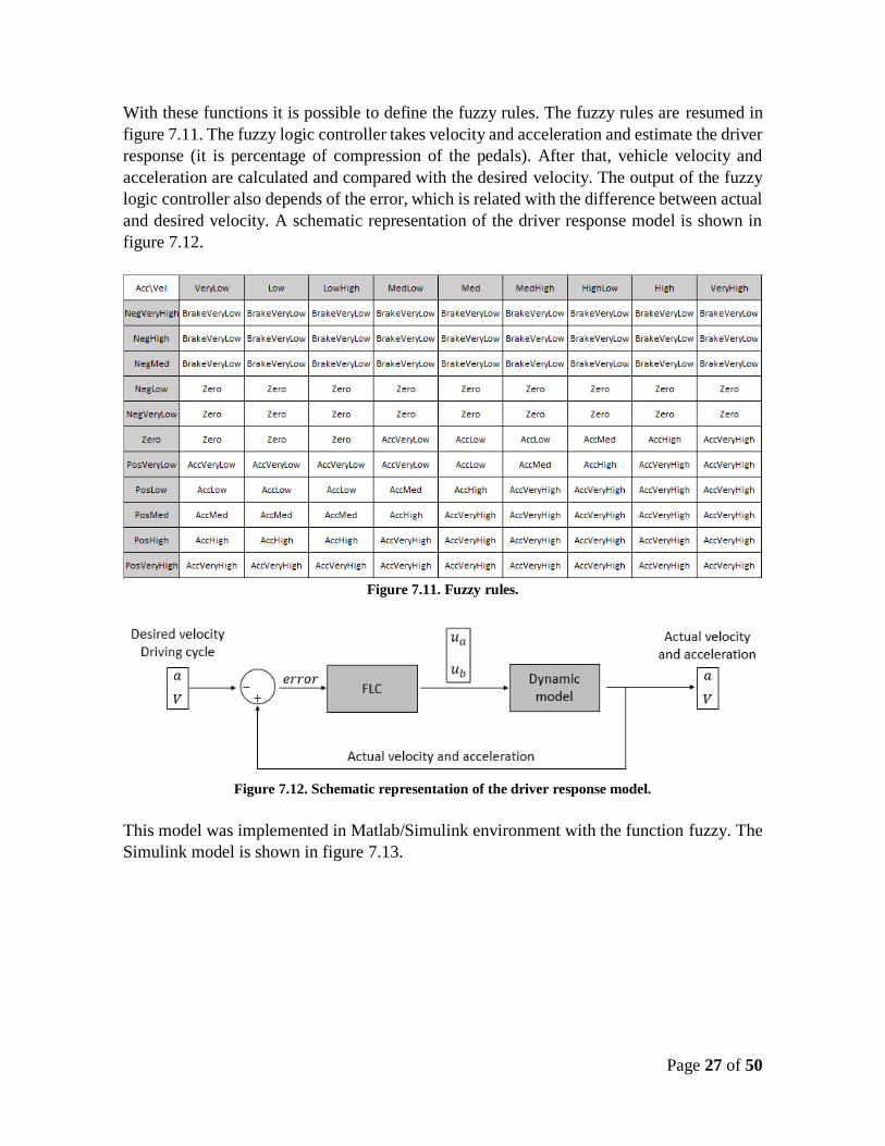
With these functions it is possible to define the fuzzy rules. The fuzzy rules are resumed in
figure 7.11. The fuzzy logic controller takes velocity and acceleration and estimate the driver
response (it is percentage of compression of the pedals). After that, vehicle velocity and
acceleration are calculated and compared with the desired velocity. The output of the fuzzy
logic controller also depends of the error, which is related with the difference between actual
and desired velocity. A schematic representation of the driver response model is shown in
figure 7.12.
Figure 7.11. Fuzzy rules.
Figure 7.12. Schematic representation of the driver response model.
This model was implemented in Matlab/Simulink environment with the function fuzzy. The
Simulink model is shown in figure 7.13.

Page 28 of 50
Figure 7.13. Simulink model of the driver response model.
This model has three inputs: acceleration, velocity and error. The output is the percentage of
compression of the pedals. The output is one of the inputs of the plant call vehicle. The model
of the plant is shown in figure 7.14.
Figure 7.14. Detail of the model of the vehicle.
In the block “Add” the sum of the terms of the equation 5.9 is done. The inputs 1 and 2 of
this block are the traction force. The input 1 is the traction force for braking and the input 2
is the traction force for moving forward. In the input 2, a linear model of the accelerator is
made. In the “Lookup Table Dynamic” the maximum tractive torque is interpolated for each
value of vehicle velocity. The data input of this “Lookup Table Dynamic” is the maximum
tractive torque as a function of the vehicle velocity. This function was made with the
assumption of a 100% efficient transmission. Once the maximum tractive torque is
calculated, this value is multiplied for the percentage of compression of the pedal. The output
of the model is the actual vehicle velocity, which is compared with the reference velocity.

Page 29 of 50
7.4 Hydraulic system control
The control system for the hydrostatic transmission must be able to maintain the transmission
in its most efficient point of operation. The most efficient point was determined in a previous
section with the instantaneous steady optimization.
The inputs of the control system must be the actual vehicle velocity, the tractive torque and
the error between the actual electric motor velocity and the ideal electric motor velocity. With
vehicle velocity and tractive torque, the optimal electric motor velocity is calculated with the
instantaneous steady optimization. The optimal value is compared with the actual value and
the fuzzy logic control adjust the system in order to be as near as possible of the optimal
value. A schematic representation of this process is shown in figure 7.15.
Figure 7.15. Schematic representation of the hydrostatic transmission control strategy.
The membership functions can be defined with the results of the instantaneous steady
optimization. The membership functions for all the inputs are shown in figures 7.16, 7.17
and 7.18. The membership functions for the output are shown in figure 7.19.
Figure 7.16. Membership functions for the tractive torque.

Page 30 of 50
Figure 7.17. Membership functions for the vehicle velocity.
Figure 7.18. Membership functions for the error.
Figure 7.19. Membership functions for the hydraulic motor displacement.
This model was implemented in Matlab/simulink environment with the function fuzzy. The
Simulink model is shown in figure 7.20.
Figure 7.20. Simulink model for the hydrostatic transmission control.
Page 31 of 50
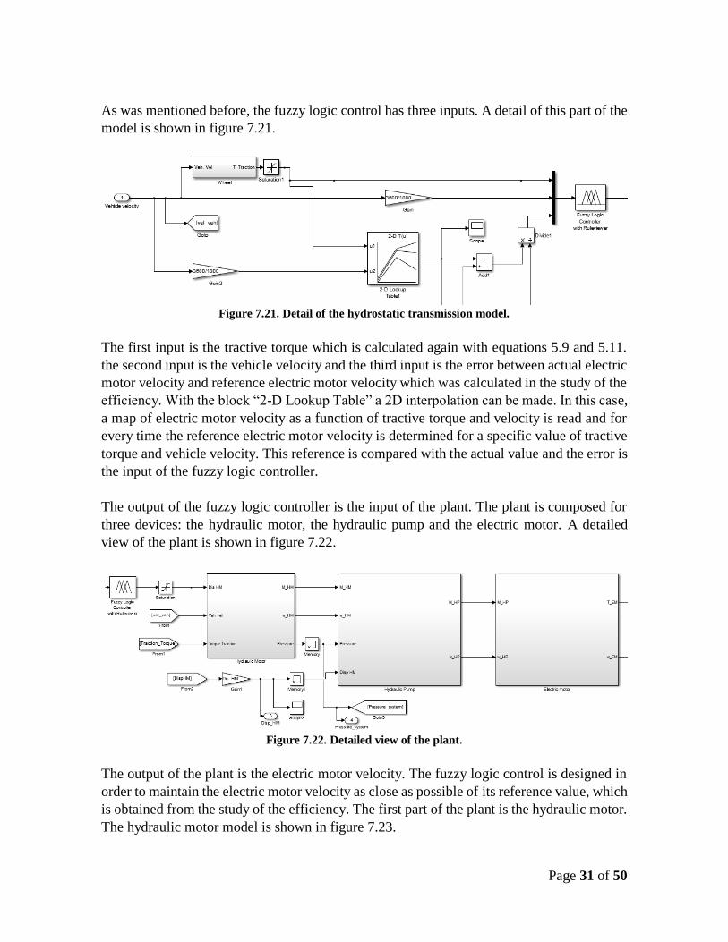
As was mentioned before, the fuzzy logic control has three inputs. A detail of this part of the
model is shown in figure 7.21.
Figure 7.21. Detail of the hydrostatic transmission model.
The first input is the tractive torque which is calculated again with equations 5.9 and 5.11.
the second input is the vehicle velocity and the third input is the error between actual electric
motor velocity and reference electric motor velocity which was calculated in the study of the
efficiency. With the block “2-D Lookup Table” a 2D interpolation can be made. In this case,
a map of electric motor velocity as a function of tractive torque and velocity is read and for
every time the reference electric motor velocity is determined for a specific value of tractive
torque and vehicle velocity. This reference is compared with the actual value and the error is
the input of the fuzzy logic controller.
The output of the fuzzy logic controller is the input of the plant. The plant is composed for
three devices: the hydraulic motor, the hydraulic pump and the electric motor. A detailed
view of the plant is shown in figure 7.22.
Figure 7.22. Detailed view of the plant.
The output of the plant is the electric motor velocity. The fuzzy logic control is designed in
order to maintain the electric motor velocity as close as possible of its reference value, which
is obtained from the study of the efficiency. The first part of the plant is the hydraulic motor.
The hydraulic motor model is shown in figure 7.23.

Page 32 of 50
Figure 7.23. Hydraulic motor model.
The inputs of the hydraulic motor model are three: the displacement of the hydraulic motor
(which is the output signal of the fuzzy logic controller), the vehicle velocity and the tractive
torque. The outputs of this model are three: the hydraulic torque in the motor, the angular
velocity of motor and the pressure of the system. The first and second inputs are calculated
with the equations of the hydraulic devices presented in a previous section. The pressure of
the system is calculated with equation 5.5.
𝑀𝑚 = Δ𝑃𝐷𝑚𝜂𝑚,𝑚 (5.5)
This equation was solved for a mesh of many values of hydraulic motor torque and
displacement. In the Matlab file sol_P_HM, the value of pressure which is the solution of
the equation for any combination of torque and displacement is saved. The solution of this
equation is used in the hydraulic motor model. With the “2-D Lookup Table” an interpolation
of the solution is made. The inputs of this table are the torque and the displacement and the
output is the pressure, which is the solution of the equation 5.5.
Before the hydraulic motor model, a subsystem with the hydraulic pump model is placed. A
detailed view of this model is shown in figure 7.24.
Page 33 of 50
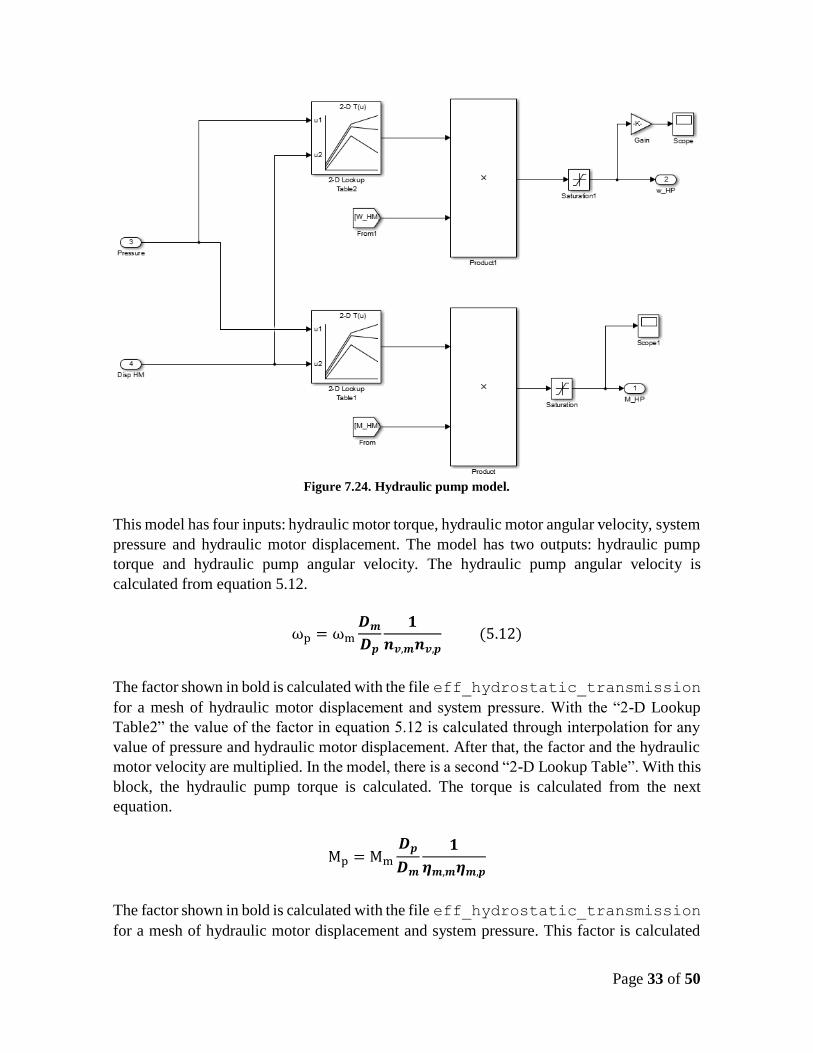
Figure 7.24. Hydraulic pump model.
This model has four inputs: hydraulic motor torque, hydraulic motor angular velocity, system
pressure and hydraulic motor displacement. The model has two outputs: hydraulic pump
torque and hydraulic pump angular velocity. The hydraulic pump angular velocity is
calculated from equation 5.12.
ωp = ωm
𝑫𝒎
𝑫𝒑
𝟏
𝒏𝒗,𝒎𝒏𝒗,𝒑 (5.12)
The factor shown in bold is calculated with the file eff_hydrostatic_transmission
for a mesh of hydraulic motor displacement and system pressure. With the “2-D Lookup
Table2” the value of the factor in equation 5.12 is calculated through interpolation for any
value of pressure and hydraulic motor displacement. After that, the factor and the hydraulic
motor velocity are multiplied. In the model, there is a second “2-D Lookup Table”. With this
block, the hydraulic pump torque is calculated. The torque is calculated from the next
equation.
Mp = Mm
𝑫𝒑
𝑫𝒎
𝟏
𝜼𝒎,𝒎𝜼𝒎,𝒑
The factor shown in bold is calculated with the file eff_hydrostatic_transmission
for a mesh of hydraulic motor displacement and system pressure. This factor is calculated

Page 34 of 50
through interpolation for any value of pressure and hydraulic motor displacement. After that,
the factor and the hydraulic motor torque are multiplied.
The last part of the plant is the electric motor. The Simulink model for the electric motor is
shown in figure 7.25.
Figure 7.25. Electric motor model.
In this model, the equations of the electric motor are solved. The inputs are the variables of
the hydraulic pump: torque and angular velocity. The outputs are angular velocity and torque
in the electric motor. This velocity is compared with the reference and the error between them
is one of the three inputs of the fuzzy logic controller.

Page 35 of 50
8. Results
The results obtained in this work are presented in this section.
8.1 Driver response model
The driver response model implemented in Simulink was tested for some conditions. The
first one is the driving cycle presented in figure 6.2. The comparison between desired velocity
and actual velocity is presented in figure 8.1. The percentage of compression for the
acceleration pedal is shown in figure 8.2.
Figure 8.1. Comparison between desired velocity and actual velocity.
Figure 8.2. Percentage of compression for the acceleration pedal.

Page 36 of 50
From figure 8.1 it is possible to see that the results for the driver response model are good.
The error for velocity is around 7%. Also, this model was tested for a square signal in order
to see its response characteristics. A comparison between reference velocity and actual
velocity is shown in figure 8.3.
Figure 8.3. Comparison between reference velocity and actual velocity.
From this figure it is possible to see that the model is able to follow the proposed driving
cycle. The percentage of compression for the acceleration pedal is shown in figure 8.4.
Figure 8.4. Percentage of compression for the acceleration pedal.

Page 37 of 50
8.2 Hydraulic transmission control
The principal objective of the control system for the hydrostatic transmission is to maintain
the system as close as possible of the most efficient point. This can be achieved controlling
the displacement of the hydraulic motor in order to change the transmission ratio for
maintaining the system in its most efficient point, which was determined with the
instantaneous steady optimization described before.
The control system was tested for the driving cycle shown in figure 6.2. A comparison
between ideal electric motor velocity and actual electric motor velocity is shown in figure
8.5.
Figure 8.5. Comparison between desired velocity and actual velocity.
From figure 8.5 it is possible to see that the control system is able to maintain the electric
motor velocity close to its most efficient point. The error is around 11%. The hydraulic motor
displacement, which is the output of the control system, is shown in figure 8.6.
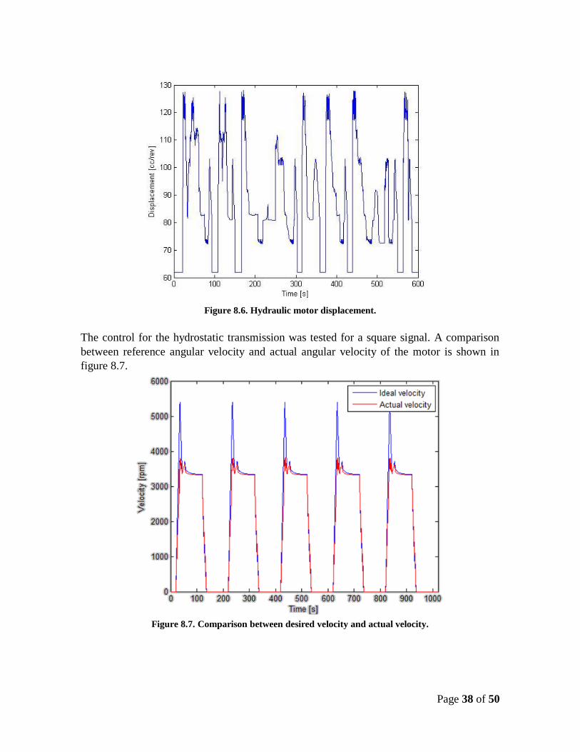
Page 38 of 50
Figure 8.6. Hydraulic motor displacement.
The control for the hydrostatic transmission was tested for a square signal. A comparison
between reference angular velocity and actual angular velocity of the motor is shown in
figure 8.7.
Figure 8.7. Comparison between desired velocity and actual velocity.

Page 39 of 50
From figure 8.7 it is possible to see that the hydraulic system control is able to maintain the
electric motor velocity very close of its reference value. The displacement of the hydraulic
motor, which is the output of the control system, is shown in figure 8.8.
Figure 8.8. Hydraulic motor displacement.
8.3 Energetic analysis
A significant increase in energy savings was achieved using the instantaneous steady
optimization. For the driving cycle shown in figure 6.2 the energy saved can be around 6%
over a hydrostatic transmission without optimization. This energy saving is due to the raise
in efficiency of all the system. With the control system, the energy saving is around 4.5%,
which is very close to the ideal energy saving. A comparison between the power consumption
of the system is shown in figure 8.9.
Figure 8.9. Power consumption.
Page 40 of 50
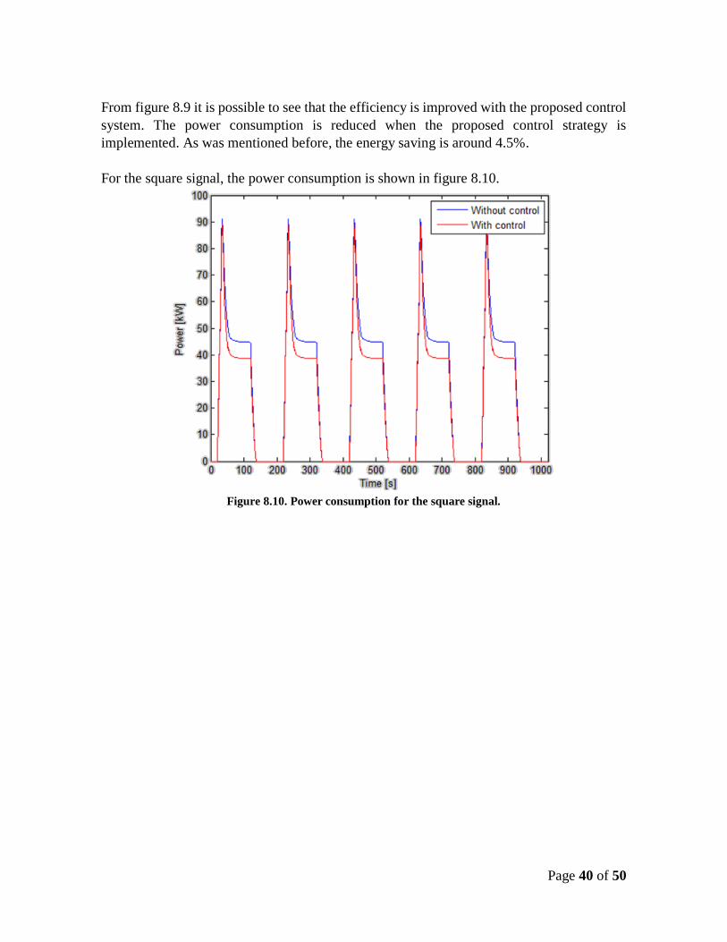
From figure 8.9 it is possible to see that the efficiency is improved with the proposed control
system. The power consumption is reduced when the proposed control strategy is
implemented. As was mentioned before, the energy saving is around 4.5%.
For the square signal, the power consumption is shown in figure 8.10.
Figure 8.10. Power consumption for the square signal.

Page 41 of 50
9. Conclusions
A numerical model was developed in order to select the components of a hydrostatic
transmission for a terrestrial commercial vehicle. The model allows to compare at the same
time many options of hydraulic components and select the component which can supply the
requirements of the vehicle for a specific driving cycle. This model takes into account
relevant characteristics of the devices such as its mass inertia and its limit capabilities.
One of the most important advantages of a hydrostatic transmission is the possibility of
adjusting the displacement of the hydraulic devices for changing the transmission ratio. This
property allows to have a continuous variable transmission. The efficiency of the hydraulic
devices depends highly of its displacements, so it is important to study their influence in the
efficiency of all the system. For this purpose, a quasi-static model was used to determine the
most efficient possible configuration of the hydrostatic transmission. For a specific value of
vehicle velocity and traction torque, all the possible configurations were evaluated through
simulation and the most efficient configuration was recorded. In figures 7.2 and 7.3 optimal
hydraulic motor displacement and optimal hydraulic pump displacement are shown. From
figure 7.3 it is possible to see that the hydraulic pump displacement is almost the same in all
regions, but the optimal hydraulic motor displacement takes many values. So, a good
hydrostatic transmission can be made with a variable displacement hydraulic motor and a
fixed displacement hydraulic pump. The optimal total efficiency of the system can reach
values of 80% for high values of tractive torque (figure 7.4), but for low values of tractive
torque the optimal efficiency is between 3% and 65% which is very low compared with a
traditional mechanical transmission. For low tractive torque values, an alternative as power
split transmission can be useful.
With an appropriate control strategy, the efficiency of the hydrostatic transmission can be
improved considerably. Through simulation, it was determined that the energy consumption
can be reduced until 6% with respect to a hydrostatic transmission without optimal control.
Using a fuzzy logic controller, the efficiency was improved 4.5%. The efficiency of the
system can be improved, as can be seen in figures 8.9 and 8.10.
Fuzzy logic control was selected as a control method because it has used successfully in
hybrid vehicles [12] [13] [14] [15]. In this work, fuzzy logic was used to model the driver
input and also it was used as a control strategy for the hydrostatic transmission.
In order to model the driver input, a computational fuzzy logic model was developed and
implemented in Simulink. The membership functions and fuzzy rules were defined according
to the figures 7.5 and 7.6, which were obtained with the dynamic model of the vehicle. The
results of this model are good. The error between desired velocity and actual velocity is
around 7%. The model can be improved adding membership functions in order to raise the
resolution.

Page 42 of 50
The results for the hydrostatic transmission control are good. The fuzzy logic controller is
able to maintain the hydrostatic transmission very close to its most efficient point. In figures
8.5 and 8.7 it is possible to see that the ideal and actual electric motor velocity are very close.
The error between them is around 11%. Moreover, the efficiency of the system is improved
through the time, as can be seen in figures 8.9 and 8.10.
Page 43 of 50
10. Future work
1. It is necessary to review the acceleration/braking model used in the driver response
model. In the present work a linear model was used, but no other models were
reviewed. The difference between reference and actual velocity in figure 8.1 can be
improved using a more realistic model.
2. In the study of the efficiency of the system in chapter 7.1, the influence of vehicle
acceleration must be studied. In the present work, a mesh of tractive torque and
velocity was made and for every possible combination of tractive torque and velocity,
the efficiency of the system was studied. As a future work, it is necessary to add the
acceleration of the vehicle as a variable. So, the efficiency will be studied for every
combination of tractive torque, vehicle velocity and acceleration.
3. In a future work it is necessary to simulate the performance of the system for an actual
driving cycle in order to have more realistic results.
4. It is necessary to compare the control strategy proposed in this work with other
control strategies in order to identify pros and cons of every possible alternative.
5. In the present work, the power consumption of the proposed system was compared
with the power consumption of a vehicle with a hydrostatic transmission without
control. In a future work, it is necessary to compare the power consumption of the
system proposed in this work with a fully electric hybrid vehicle.
6. In a future work it is necessary to add the model of the regenerative braking and the
accumulator. Also, it is necessary to review the braking model proposed in the present
work.
7. Alternatives as power split transmission must be studied and evaluated in order to
improve the efficiency of the system for low values of tractive torque.

Page 44 of 50
11. Bibliography
[1] S. Davis, Diegel, S. and R. Boundy, Transportation Energy Data Book: Editiom 33
(No. ORNL 6990), 2014.
[2] M. Ehsani, Y. Gao, S. Gay and A. Emadi, Modern Electric, Hybrid Electric, and Fuel
Cell Vehicles, Florida: CRC Press, 2005.
[3] M. Ivantysynova and M. Sprengel, “Investigation and Energetic Analysis of a Novel
Hydraulic Hybrid Architecture for On-Road Vehicles,” in The 13th Scandinavian
International Conference on Fluid Power, Linkping, Sweden, 2013.
[4] M. Heskitt, T. Smith and J. Hopkins, “Design & Development of the LCO-140H Series
Hydraulic Hybrid Low Floor Transit Bus,” BUSolutions Final Technical Report, no.
No. FTA Report No. 0018, 2012.
[5] N. Clark, F. Zhen, W. Wayne and D. Lyons, “Transit Bus Life Cycle Cost and Year
2007 Emissions Estimation,” no. FTA-WV-26 7004.2007.1.
[6] B. Wu, C. C. Lin, Z. Filipi, H. Peng and D. Assanis, “Optimal Power Management for
a Hydraulic Hybrid Delivery Truck,” Vehicle System Dynamics, no. 42, pp. 23-40,
2004.
[7] F. Bender, T. Bosse and O. Sawodny, “An investigation on the fuel savings potential
of hybrid hydraulic refuse collection vehicles,” Waste Management, 2014.
[8] M. Sprengel, T. Bleazard, H. Haria and M. Ivantysynova, “Implementation of a Novel
Hydraulic Hybrid Powertrain in a Sports Utility Vehicle,” International Federation of
Automatic Control, pp. 187-194, 2015.
[9] A. Rajagolapan, “Development of Fuzzy Logic and Neural Network Control and
Advanced Emissions Modeling for Parallel Hybrid Vehicles,” 2003. [Online].
Available: http://www.ctts.nrel.gov/analysis/readingroom.html.
[10] B. M. Baumann, “Mechatronic Design and Control of Hybrid Electric Vehicles,”
IEEE/ASME Transactions on Mechatronics, vol. 1, no. 5, pp. 58-72, 2000.
[11] P. Mathenson and J. Stecki, “Modeling and Simulation of a Fuzzy Logic Controller for
a Hydraulic-Hybrid Powertrain for Use in Heavy Commercial Vehicles,” in Powertrain
and Fluid Systems Conference and Exhibition, Pittsburgh, Pennsylvania, 2003.
[12] N. Jalil and N. Kheir, “Energy Management Studies for a New Generation of Vehicles
(Milestone No.5: Fuzzy logic for the series hybrid),” Oakland, 1998.
[13] N. Jalil and N. Kheir, “Energy Management Studies for a New Generation of Vehicles
(Milestone No.6: Fuzzy logic for the parallel hybrid),” Oakland, 1998.
[14] B. M. Baumann, “Intelligent control strategies for hybrid vehicles using neural
networks and fuzzy logic, Masters thesis, Dept. Elect. Eng., Ohio State Univ.,”
Columbus, 1997.
[15] H. Kono, “Fuzzy contro for hybrid electric vehicles, Master thesis, Department of
Electrical Engineering, The Ohio State University,” Columbus, 1998.
Page 45 of 50
[16] N. Schouten, M. Salman and N. Kheir, “Fuzzy Logic Control for Parallel Hybrid
Vehicles,” IEEE Transactions on Control Systems Technology, vol. 10, no. 3, 2002.
[17] M. Sprengel, T. Bleazard, H. Haria and M. Ivantysynova, “Optimal Contrl and
Performance Based Design of the Blended Hydraulic Hybrid,” in ASME/BATH 2015
Symposium on Fluid Power and Motion Control, Chicago, Illinois, 2015.
[18] M. Sprengel and M. Ivantysynova, “Recent Developments in a Novel Blended
Hydraulic Hybrid Transmission, SAE Technical Paper 2014-01-2399,” in SAE 2014
Commercial Vehicle Engineering Congress, Rosement, IL, USA, Oct. 7-9, 2014.
[19] J. Leon, J. Garcia, M. Acero, A. Gonzalez, G. Niu and M. Krishnamurthy, “Case Study
of an Electric-Hydraulic Hybrid Propulsion System for a Heavy Duty Electric Vehicle,
SAE Technical Paper No. 2016-01-8112,” in SAE 2016 Commercial Vehicle
Engineering Congress, Rosemont, IL, USA, 2016.
[20] L. C. Belalcazar, H. Acevedo and N. Rojas, “Construcción de ciclos de conducción de
Bogotá para la estimación de factores de emisión vehiculares y consumos de
combustible,” Bogotá, 2013.
[21] C. Wang, W. Yijun and O. Jiajie, “Simulation of fuzzy control strategy for parallel
hybrid electric vehicle,” in Electric and control engineering (ICEICE), 2011
International Conference, 2011.
[22] H. D. Lee, E. S. Koo, S. K. Sul and J. S. Kim, “Torque Control Strategy for a Parallel
Hybrid Vehicle Using Fuzzy Logic,” IEEE Industry Applications Magazine, pp. 33-38,
2000.
[23] I. A. Njabeleke, R. F. Pannett, P. K. Chawdhry and C. R. Burrows, “Self Organising
Fuzzy Logic Control of a Hydrostatic Transmission,” in UKACC International
Conference on Control, 1998.
[24] T. Gillespie, Fundamentals of Vehicle Dynamics, Society of Automotive Engineers,
Inc., 1992.

Page 46 of 50
Appendix
In this appendix, an explanation about using the Matlab/Simulink simulations is made. Next,
all the Matlab files are explained.
File name Function
Torque_traction.m
The maximum traction torque that the electric
motor can provide for a specific vehicle velocity.
This traction torque is calculated with the
assumption of a 100% efficiency of the
transmission. This file need the electric motor
data. The data file has three columns. The first one
is the angular velocity in rpm, the second one is
the maximum torque and the last one is the
maximum power.
Driving_cycle.m
The driving cycle used as a reference is calculated
in this file. Also, this file is used for reading the
results of the study of the efficiency of the system.
eff_hydrostatic_transmission.m
With this file the hydrostatic transmission
efficiency is calculated for all possible values of
pressure and displacement. Also, the next numbers
are calculated:
Factor_HP_Torque
Mp = Mm
𝑫𝒑
𝑫𝒎
𝟏
𝜼𝒎,𝒎𝜼𝒎,𝒑
Factor_HP_Vel
ωp = ωm
𝑫𝒎
𝑫𝒑
𝟏
𝜼𝒗,𝒎𝜼𝒗,𝒑
EM_eff.m
The efficiency map for the electric motor is
generated in this filed.
sol_P_HM.m
The pressure is solved for every possible value of
displacement and hydraulic motor torque. The
equation solved is the next:

Page 47 of 50
𝑀𝑚 = Δ𝑃𝐷𝑚𝜂𝑚,𝑚
vehicle.m
The vehicle variables are described in this file. All
the files are written for reading the variables from
this file.
hydrostatic_transmission.m
The hydrostatic transmission variables are
described in this file. All the files are written for
reading the variables from this file.
efficiency_HP.m
This function has as inputs the pressure (bar) and
displacement (0 - 1) and the output is a vector with
three positions: the first position is the total
efficiency, the second position is the volumetric
efficiency and the last position is the mechanical
efficiency.
efficiency_HM.m
This function has as inputs the pressure (bar) and
displacement (0 - 1) and the output is a vector with
three positions: the first position is the total
efficiency, the second position is the volumetric
efficiency and the last position is the mechanical
efficiency.
efficiency_EM.m
This function has as inputs the torque (Nm) and
the angular velocity (rpm) and the output is the
electric motor efficiency (0 - 100).
optimization.m
The study of the efficiency of the system is made
with this file. The computational cost associated
with this file is big.
Controller_v4
The Simulink models for the human response and
the hydrostatic transmission are in this file.
For running the simulation, it is necessary to run the files in the next order:
1. Torque_traction.m

Page 48 of 50
2. Driving_cycle.m
3. eff_hydrostatic_transmission.m
4. EM_eff.m
After that, it is necessary to open the fuzzy logic dialog box with the function fuzzy in the
command window. The fuzzy logic dialog box has the next view.
In this dialog box, it is necessary to charge the files of the membership functions and the
fuzzy rules. For doing that, click on File/Import/From File… and the file must be selected.
When the file has been selected, the dialog box has the next view.

Page 49 of 50
The inputs are on the left and the output is on the right. For modifying the membership
functions, double click on one of the inputs. A new dialog box is open.

Page 50 of 50
Once the fuzzy functions have been charged, the simulation can be run in Simulink. Before
running these files, it is necessary to have the results for the study of the efficiency obtained
with the file optimization.m and also it is necessary to have the solution of the pressure
from file sol_P_HM.m.