A fully divergence-free finite element method for magneto-hydrodynamic ... A fully divergence-free...

A fully divergence-free finite element

method for magneto-hydrodynamic

equations

R. Hiptmair and L.-X. Li and S.-P. Mao and W.-Y. Zheng

Research Report No. 2017-25May 2017

Seminar für Angewandte MathematikEidgenössische Technische Hochschule

CH-8092 ZürichSwitzerland

____________________________________________________________________________________________________

Funding: This work is supported in part by the National Center for Mathematics and Interdisciplinary Sciences of China, the State

Key Laboratory of Scientific and Engineering Computing of China, and National Magnetic Confinement Fusion Science Program of

China (2015GB110003). S. Mao is supported by the National Key Research and Development Program of China

(2016YFB0201304), China NSF 11471329, and Youth Innovation Promotion Association of CAS (2016003). W. Zheng is

supported by China NSF under the Grant 91430215.

A FULLY DIVERGENCE-FREE FINITE ELEMENT METHOD FOR

MAGNETOHYDRODYNAMIC EQUATIONS

RALF HIPTMAIR

Seminar of Applied Mathematics, Swiss Federal Institute of Technology

Zurich, CH-8092, Switzerland

[email protected]

LINGXIAO LI

Academy of Mathematics and System Sciences, Chinese Academy of Sciences

School of Mathematical Science, University of Chinese Academy of Sciences

Beijing, 100190, China

[email protected]

SHIPENG MAO




[email protected]

WEIYING ZHENG




[email protected]

In this paper, a fully divergence-free finite element method is proposed to solve three-dimensional incompressible magnetohydrodynamic equations. The main merit of themethod is that the spatial discretization ensures that the approximations of the ve-locity and the magnetic induction are divergence-free exactly. We employ second-ordersemi-implicit timestepping, for which we rigorously establish an energy law and, as aconsequence, unconditional stability. We prove unique solvability of the linear systemof equations to be solved in every timestep. To solve them, we propose an efficient pre-conditioner so that the number of preconditioned GMRES iterations is uniform withrespect to the number of degrees of freedom. Moreover, by several numerical experi-ments, we confirm the predictions of the theory and demonstrate the efficiency of the

preconditioner.

Keywords: Magnetohydrodynamic equations; divergence-free finite element method; pre-conditioner; magnetic vector potential; driven cavity flow.

AMS Subject Classification: 65M60, 76W05

1

2 R. Hiptmair et al.

1. Introduction

The incompressible magnetohydrodynamic (MHD) equations describe the dynamic

behavior of an electrically conducting fluid under the influence of a strong mag-

netic field. They occur in models for, fusion reactor blankets, liquid metal magnetic

pumps, aluminum electrolysis among others (see Ref. 1 and 23). MHD is a multi-

physics phenomenon: the magnetic field changes the momentum of the fluid through

the Lorenz force, and conversely, the conducting fluid influences the magnetic field

through electric currents. In this way multiple physical fields, such as the velocity,

the pressure, and the electromagnetic fields, are coupled.

In this paper, we study the incompressible MHD equations in a bounded do-

main Ω ⊂ R3 which consist of the incompressible Navier-Stokes equations and the

magnetoquasistatic Maxwell’s equations

∂u

∂t+ (u · ∇)u− J ×B +∇p− ν∆u = f in Ω, (1.1a)

∂B

∂t+ curlE = 0 in Ω, (1.1b)

curlH = J in Ω, (1.1c)

divu = 0, divB = 0 in Ω, (1.1d)

where u is the fluid velocity, p is the hydrodynamic pressure, E is the electric field,

H is the magnetic field, B is the magnetic induction, J is the electric current

density, and f ∈ L2(Ω) stands for the source field. The equations in (1.1) are

complemented with the following constitutive equation and Ohm’s law

B = µH, J = σ(E + u×B). (1.2)

The physical parameters are, respectively, the kinematic viscosity ν, the magnetic

permeability µ, and the electric conductivity σ. For the well-posedness of (1.1) and

(1.2), we assume the following initial and boundary conditions

u(0) = u0, B(0) = B0 in Ω,

u = 0, E × n = 0 on Γ := ∂Ω.(1.3)

Numerical methods for incompressible MHD equations has been studied widely.

For the stationary model, we refer to Ref. 9, 13, 14, and 27 for stabilized and

mixed finite element methods. In Ref. 14, the authors proved optimal error esti-

mates for H1(Ω)-conforming finite element approximations both to velocity u and

magnetic induction B in either polyhedra or domains with C1,1-smooth bound-

aries. It is well-known that B may not be in H1(Ω) in general Lipschitz domains

which are not convex. In Ref. 27, Schotzau proved the well-posedness of stationary

MHD equations and studied a mixed finite element method which discretizes u

with H1(Ω)-conforming finite elements and B with H(curl,Ω)-conforming finite

elements. The mixed finite element method yields a discrete magnetic induction

Bh which is weakly divergence free, that is, Bh is orthogonal to all discrete gra-

dient fields. In Ref. 12, Greif, Li, Schotzau, and Wei extended the framework by

Divergence-free FEM for MHD equations 3

focusing on the conservation of mass, namely, divu = 0. They proposed a mixed

discontinuous Galerkin (DG) finite element method for the stationary MHD model

and discretized u in an H(div,Ω)-conforming finite element space. The merit of

the method is that the discrete velocity satisfies divuh = 0 exactly.

In recent years, exactly divergence-free approximations for B have attracted

more and more interests for the spatial discretization of the time-dependent MHD

equations, particularly, in the development of a simulation code for fusion reactor

blanket (cf. Ref. 1–2). For instance, Ni et al developed current density-conservative

finite volume methods for a simplified MHD model on both structured and unstruc-

tured grids (cf. Ref. 25, 26, 29, 31). Their methods are efficient for high Hartmann

numbers and have been validated by experimental results. In Ref. 18, the authors

proposed a stable finite element method for incompressible MHD equations which

preserves divBh = 0 exactly. In contrast to most existing approaches that eliminate

the electrical field variable E and give a direct discretization of the magnetic field,

they discretizes the electric field E by Nedelec’s edge elements and discretizes the

magnetic induction B by Raviart-Thomas face elements. In this way, divBh = 0

is ensured exactly for the discrete solution. In Ref. 19, they also proposed a robust

preconditioner for solving the discrete problem.

The purpose of this paper is to propose a new mixed DG finite element method

for solving (1.1). Inspired by Ref. 12, we approximate the velocity u by H(div,Ω)-

conforming finite elements and the pressure p by fully discontinuous finite elements.

As a result, the conservation of mass is satisfied on the discrete level, that is,

divuh = 0 holds exactly. The divergence-free property of B is realized by means of

a magnetic vector potential. Instead of solving for (E,B), we solve for the magnetic

vector potential A under the temporal gauge so that

E = −∂A

∂t, B = curlA.

Approximating the vector magnetic potential by H(curl,Ω)-conforming edge ele-

ments and defining Bh = curlAh, we find that divBh = 0 holds naturally and

exactly. We say the mixed finite element method is fully divergence-free in the sense

that both the discrete velocity and the discrete magnetic induction satisfy exactly

divuh = 0, divBh = 0.

The second objective is to propose an efficient solver for the discrete problem.

We propose a linearized discrete problem at tn by using the extrapolation of the

discrete solutions at tn−1 and tn−2. We need only solve a linear discrete problem at

each time step. Existence and uniqueness of its solution can be shown and a discrete

energy law holds for the fully discrete scheme. Numerical experiments show that the

extrapolated scheme is second order in time. This means that the proposed method

is stable and efficient for long-time simulation of MHD problems.

We also propose a preconditioner for solving the linear systems of equations in

each timestep. The optimality of the preconditioner is verified numerically with re-

spect to the number of degrees of freedom (DOFs). Extensive numerical experiments


are presented to verify the convergence rate of the mixed finite element method and

the optimality of the preconditioner, to demonstrate the competitive performance of

the linear extrapolated scheme, and to validate the A-based MHD formulation for

an engineering benchmark problem. Furthermore, our numerical results well match

the two-dimensional simulations for a driven cavity flow in Ref. 20.

The paper is organized as follows: In Section 2, we introduce the MHD model

which uses the velocity, the pressure, and the vector magnetic potential as un-

knowns. A weak formulation is proposed and the energy law of the solutions is

proved. In Section 3, we propose a fully discrete mixed DG finite element method

for solving the weak MHD formulation using the extrapolation of the solutions at

previous time steps. The energy law of the discrete solutions is also proved under

discrete norms. In Section 4, we introduce the preconditioned GMRES algorithm

for solving the discrete problem. In Section 5, we present four numerical experi-

ments to confirm the prediction of the theory and to demonstrate the competitive

behavior of the MHD solver.

2. A weak formulation of the MHD model

The purpose of this section is to derive a weak formulation of the MHD system

(1.1) based on the vector magnetic potential. An energy law for the solutions is

also proved. Throughout the paper, we assume that Ω ⊂ R3 is a bounded Lipschitz

polyhedral domain with boundary Γ = ∂Ω. For simplicity, we assume that the

density of fluid ρ ≡ 1 and the physical parameters µ, σ, ν are positive constants.

Moreover, vector-valued quantities will be denoted by boldface notation, such as

L2(Ω) := (L2(Ω))3.

Let L2(Ω) be the space of square-integrable functions and let its inner product

and norm be denoted by

(u, v) :=

∫

Ω

uv, ‖u‖L2(Ω) := (u, u)1/2.

We shall also use the usual Hilbert spaces like H1(Ω), H(curl,Ω), H(div,Ω) and

their subspaces H10 (Ω), H0(curl,Ω), H0(div,Ω) with vanishing traces, vanishing

tangential traces, and vanishing normal traces on Γ respectively. We refer to Chap-

ter 3 in Ref. 22 for their definitions and inner products. The subsapces of curl-free

functions and divergence-free functions are denoted by

H(div 0,Ω) := v ∈H(div,Ω) : div v = 0,

H(curl 0,Ω) := v ∈H(curl,Ω) : curlv = 0.

Since divB = 0, we can introduce a magnetic vector potential A and write

E = −∂tA, B = curlA in Ω, (2.1)

where the temporal gauge is adopted for convenience. With the abbreviations ∂tu =


∂u∂t and ∂tA = ∂A

∂t , (1.1) can be written as follows

∂tu+ (u · ∇)u− J × curlA+∇p− ν∆u = f in Ω,

divu = 0 in Ω,

σ (∂tA+ curlA× u) + curlµ−1 curlA = 0 in Ω,

−σ (∂tA+ curlA× u) = J in Ω.

Using (1.3) and (2.1), it suffices to set the initial condition for A by solving the

static problem

curlA0 = B0, divA0 = 0 in Ω,

A0 × n = 0 on Γ.

The boundary condition for A can also be obtained by combining (1.3) and (2.1)

A× n = A0 × n−

∫ t

0

(E × n) = 0 on Γ.

For simplicity, let U0, B0, L0 be the characteristic quantities for velocity, mag-

netic induction, length of the system respectively. We introduce the following nondi-

mensionalization

x← x/L0, t← tU0/L0, A← A/(B0L0), f ← fL0/U20 , p← p/U2

0 .

The MHD system can be written in a dimensionless form

∂tu+ u · ∇u+∇p−R−1e ∆u− κJ × curlA = f in Ω, (2.3a)

divu = 0 in Ω, (2.3b)

∂tA+ curlA× u+R−1m curl curlA = 0 in Ω, (2.3c)

−∂tA− curlA× u = J in Ω, (2.3d)

u(0) = u0, A(0) = A0 in Ω, (2.3e)

u = 0, A× n = 0 on Γ, (2.3f)

where Re = L0U0/ν is the Reynolds number, Rm = µσL0U0 is the magnetic

Reynolds number, and κ = σB20L0/U0 is the coupling number between the fluid

and the magnetic field.

Now we derive a weak formulation of (2.3). For convenience, we introduce some

notations for the function spaces

V =H10(Ω) ∩H(div 0,Ω), C =H0(curl,Ω).

Multiply both sides of (2.3a) with v ∈ V . Using integration by part and noting

v = 0 on Γ, we have

(∂tu+ u · ∇u− κJ × curlA,v)− (p, div v) +R−1e (∇u,∇v) = (f ,v).

Using div v = 0 and substituting (2.3d) into the above equality, we get

(∂tu+ u · ∇u,v) + κ(∂tA+ curlA× u, curlA× v) +R−1e (∇u,∇v) = (f ,v).


Similarly, multiplying both sides of (2.3c) with ϕ ∈ C, using integration by part,

and noting ϕ× n = 0, we have

(∂tA+ curlA× u,ϕ) +R−1m (curlA, curlϕ) = 0.

Then we get a weak formulation of (2.3): Find u ∈ V , A ∈ C such that A(0) = A0,

u(0) = u0, and

(∂tu,v) +O(u;u,v) +A(u,v) + κ(∂tA+B × u,B × v) = (f ,v) ∀v ∈ V ,

(2.4a)

(∂tA+B × u,ϕ) +R−1m (curlA, curlϕ) = 0 ∀ϕ ∈ C, (2.4b)

where B = curlA and

O(w;u,v) = ((w · ∇)u,v) , A(v,w) = R−1e (∇v,∇w).

Using (2.3a), the pressure can be recovered by solving the Poisson equation: Find

p ∈ H1(Ω)/R such that

(∇p,∇q) = (f + J × curlA,∇q)−O(u;u,∇q) ∀ q ∈ H1(Ω)/R. (2.5)

Theorem 2.1. Let u, A be the solutions of (2.4) and assume

u ∈ L∞(0, T ;L2(Ω)) ∩L2(0, T ;V ),

A ∈H1(0, T ;L2(Ω)) ∩L∞(0, T ;C),

J ∈ L2(0, T ;L2(Ω)).

Then the energy law holds

E(T ) +

∫ T

0

P(t)dt = E(0) +

∫ T

0

(f ,u),

where

E(t) :=1

2‖u‖

2L2(Ω) +

κ

2Rm‖B‖

2L2(Ω) , P(t) :=

1

Re‖∇u‖

2L2(Ω) + κ ‖J‖

2L2(Ω) .

Proof. For any w ∈ V , since divw = 0, direct calculations show that∫

Ω

(w · ∇)u · v = −

∫

Ω

(w · ∇)v · u ∀v ∈H10(Ω).

This means that O(w;u,u) = 0. Since ∂tA,J ∈ L2(0, T ;L2(Ω)), we have B×u ∈

L2(0, T ;L2(Ω)). Taking v = u in (2.4a) shows that

1

2

d

dt‖u‖

2L2(Ω) − κ(J ,B × u) +

1

Re‖∇u‖

2L2(Ω) = (f ,u). (2.6)

Furthermore, taking ϕ = ∂tA in (2.4b), we also have

1

2Rm

d

dt‖B‖

2L2(Ω) = (J , ∂tA) = −‖J‖

2L2(Ω) − (J ,B × u) . (2.7)

Substituting (2.7) into (2.6) yields the result.


Remark 2.1. The energy law describes the variation of the total energy caused by

energy transformation and the work of external forces. The total energy E consists

of the fluid kinetic energy 12 ‖u‖

2L2(Ω) and the magnetic field energy κ

2Rm‖B‖

2L2(Ω).

The dissipation of the total energy stems from the friction losses R−1e ‖∇u‖

2L2(Ω) and

the Ohmic losses κ ‖J‖2L2(Ω). The energy supply from external sources is represented

by (f ,u).

3. An interior-penalty finite element method

In this section, we study the fully discrete approximation to the MHD equations.

The velocity u shall be discretized by H(div,Ω)-conforming finite elements with

interior penalties in a DG-type approach. We refer to Ref. 12 for the interior-penalty

finite element method for the H-based formulation of stationary MHD model.

3.1. Finite element spaces

Let Th be a shape-regular tetrahedral triangulation of Ω and let Fh be the set of

all element faces of Th. The H10 (Ω)-conforming finite element space of piecewise

quadratic polynomials is defined by

Uh = v ∈ H10 (Ω) : v|K ∈ P2(K), K ∈ Th,

where Pk(K) is the space of polynomials with degrees no more than k ≥ 0. We

also use the notation P k(K) = Pk(K)3. The linear H0(div,Ω)- and H0(curl,Ω)-

conforming finite element spaces are defined respectively as follows (c.f. Ref. 24,

28):

V h = v ∈H0(div,Ω) : v|K ∈ P 1(K), K ∈ Th,

Ch = v ∈H0(curl,Ω) : v|K ∈ P 1(K), K ∈ Th.

For convenience, we denote the divergence-free subspace of V h as follows

V h(div 0) := V h ∩H(div 0,Ω).

Now we introduce the notations associated with traces. We endow each F ∈ Fh

with a unit normal nF which points to the exterior of Ω when F ⊂ Γ. For any

interior face F ∈ Fh, let K+, K− be two adjacent elements of Th such that F =

∂K+ ∩K− ∈ Fh. We always assume that nF points to the exterior of K+. Let ϕ

be a scalar-, vector-, or matrix-valued function which is piecewise smooth over Th.

The mean value and jump of ϕ on F are defined respectively by

ϕ :=1

2(ϕ+ + ϕ−) , JϕK := ϕ+ − ϕ− on F,

where ϕ± denote the traces of ϕ on F from inside of K± respectively. For any face

F = ∂K+ ∩ Γ with K+ ∈ Th, the mean value and the jump of ϕ on F are defined

by

ϕ = JϕK = ϕ+ on F,


We shall use the discrete semi-norm and norms

‖u‖0,h :=

(

∑

F∈Fh

h−1F ‖u‖

2L2(F )

)1

2

, |u|1,h :=

(

∑

K∈Th

‖∇u‖2L2(K)

)1

2

,

‖u‖1,h :=(

|u|21,h + ‖JuK‖

20,h

)1

2

.

We shall also use the space of piecewise regular functions

H1(Th) :=

v ∈ L2(Ω) : v|K ∈H1(K), K ∈ Th

,

V (h) := V + V h .

Apparently the embedding relationship holds

V (h) ⊂H1(Ω) + V h ⊂H1(Th).

Lemma 3.1. For any 2 ≤ p ≤ 6, there exists a constant C(p) > 0 independent of

the mesh size such that

‖v‖Lp(Ω) ≤ C(p) ‖v‖1,h ∀v ∈ V (h) . (3.1)

Proof. The inequality is proved for two-dimensional case in Lemma 6.2 of Ref. 11.

In fact, a careful inspection of its proof shows that it also applies to three-

dimensional case. We do not elaborate on the details. For p = 2, we also refer

to Ref. 4 and 6.

The discrete counterparts of the bilinear and trilinear forms are defined by

Ah(v,w) =1

Re

∑

K∈Th

∫

K

∇v : ∇w +α

Re

∑

F∈Fh

h−1F

∫

F

JuK · JvK

−1

Re

∑

F∈Fh

∫

F

(

∂u

∂n

· JvK +

∂v

∂n

· JuK

)

,

Oh(w;u,v) = −∑

K∈Th

∫

K

u · div(w ⊗ v) +∑

K∈Th

∫

∂K

(w · nK)(

u↓ · v)

,

where α > 0 is the penalty parameter independent of the mesh, nK is the unit outer

normal of ∂K, nF is the unit normal of nF , and u↓ denotes the upwind convective

flux defined by Ref. 8, 12

u↓(x) =

limε→0+

u(x− εw(x)), x ∈ ∂K\Γ,

0, x ∈ ∂K ∩ Γ.

The following lemma states that the discrete bilinear form Ah(·, ·) is coercive on

V h.


Lemma 3.2. Suppose α is large enough but independent of hF , Re, and Rm. Then

there exists a constant θ1 > 0 independent of hF , Re, and Rm such that

Ah(vh,vh) ≥θ1Re‖vh‖

21,h ∀v ∈ V h.

Proof. The proof is standard. We present it here for completeness. By the norm

equivalence on finite dimensional space (cf. Lemma A.6 in Ref. 11), there exists a

constant C1 independent of h such that

hF ‖∇vh‖2L2(F ) ≤ C1 ‖∇vh‖

2L2(KF ) ∀F ∈ Fh,

where KF ∈ Th satisfies F ⊂ ∂KF . Therefore

ReAh(v,v) = |v|21,h + α ‖JvK‖

20,h − 2

∑

F∈Fh

∫

F

∂v

∂n

· JvK

≥ |v|21,h + (α− 2C2

1 ) ‖JvK‖20,h−

1

2C1

∑

F∈Fh

hF ‖∇v‖2L2(F )

≥1

2|v|

21,h + (α− 2C2

1 ) ‖JvK‖20,h .

We complete the proof by setting α > 2C21 and θ1 := min(1/2, α− 2C2

1 ).

Lemma 3.2 states that Ah(·, ·) is coercive on H1(Th). It forms an equivalent

norm

‖v‖Ah:=√

Ah(v,v) ∀v ∈H1(Th).

We cite Ref. 8 for the following lemma on the positivity and continuity of the

trilinear form O. The proof is omitted here.

Lemma 3.3. Let w,w1 ∈H1(Th) ∩H(div 0,Ω), u ∈ V (h), and v ∈ V h. Then

Oh(w;v,v) =1

2

∑

F∈Fh

∫

F

|w · n| |JvK|2.

Furthermore, there exists a constant C0 independent of the mesh size such that

|O(w;u,v)−O(w1;u,v)| ≤ C0 ‖w −w1‖1,h ‖u‖1,h ‖v‖1,h .

3.2. A semi-implicit time-stepping scheme

Now we study the fully discrete approximation to the MHD equations. Let tn =

nτ : n = 0, 1, · · · , N, τ = T/N , be an equidistant partition of the time interval

[0, T ]. For a sequence of functions vn, we define the finite difference operator and

mean values by

δtvn :=vn − vn−1

τ, vn :=

vn + vn−1

2, (3.2)

fn :=1

6

[

f(tn) + 4f(tn−1/2) + f(tn−1)]

.


Let uh0 , A

h0 be quasi-interpolations of the initial conditions u0 ∈ H

10(Ω), A0 ∈

H0(curl,Ω) onto the finite element spaces V h andCh respectively (cf. e.g. Ref. 17).

Without causing confusion, we shall drop the superscripts and denote by u0 ∈ V h,

A0 ∈ Ch the discrete initial values.

The Crank-Nicolson scheme for the fully discrete approximation of (2.4) reads:

Find (un,An) ∈ V h(div 0)×Ch, n ≥ 0, such that

(δtun,v) +Oh(un; un,v) +Ah(un,v) + κ(δtAn + Bn × un, Bn × v) = (fn,v),

(3.3a)(

δtAn + Bn × un,ϕ)

+R−1m (curl An, curlϕ) = 0, (3.3b)

for all (v,ϕ) ∈ V h(div 0) × Ch, where Bn = curl An. It is well-known that the

Crank-Nicolson scheme is of second order with respect to τ . The discrete problem

is nonlinear and expensive to solve at each time step. Thus, inspired by Ref. 3 and

30, we consider the linearly extrapolated solutions

u∗ =1

2(3un−1−un−2), B∗ =

1

2(3Bn−1−Bn−2) =

1

2curl(3An−1−An−2). (3.4)

The truncation errors for the above approximations are of second order. For any

smooth function v, let vn = [v(tn) + v(tn−1)]/2 and v∗ = [3v(tn−1) − v(tn−2)]/2.

Then

v∗ − vn =1

2[v(tn−2) + v(tn)− 2v(tn−1)] = vtt(tn−1)τ

2 +O(τ3). (3.5)

Linearize the nonlinear terms in (3.3) by replacing un, Bn with u∗, B∗ for n ≥ 2

and with u0, A0 for n = 1. We get the semi-implicit time-stepping scheme for (2.4):

Find (un,An) ∈ V h(div 0)×Ch, n ≥ 2, such that, for any (v,ϕ) ∈ V h(div 0)×

Ch,

(δtun,v) +Oh(u∗; un,v) +Ah(un,v) + κ(δtAn +B∗ × un,B∗ × v) = (fn,v),

(3.6a)

(δtAn +B∗ × un,ϕ) +1

Rm(curl An, curlϕ) = 0. (3.6b)


Theorem 3.1. The discrete problem (3.6) has a unique solution in each time

step. The discrete energy law holds

En − En−1

τ+ Pn = (fn, un) ∀n ≥ 1, (3.7)

where

En :=1

2‖un‖

2L2(Ω) +

κ

2Rm‖curlAn‖

2L2(Ω) ,

Pn := ‖un‖2Ah

+1

2

∑

F∈Fh

∫

F

|u∗ · n| |JunK|2+ κ ‖δtAn +B∗ × un‖

2L2(Ω) .

Proof. We first prove the discrete energy law. Let Jn := −δtAn−B∗× un be the

discrete electric current density. Taking v = un in (3.6a) yields

(δtun, un) +Oh(u∗; un, un) +Ah(un, un) = κ (Jn,B∗ × un) + (fn, un). (3.8)

Since un ∈ V h ∩H(div 0,Ω), from Lemma 3.3 we have

Oh(u∗; un, un) =1

2

∑

F∈Fh

∫

F

|u∗ · n| |JunK|2.

Furthermore, by taking ϕ = δtAn in (3.6b), we find that

1

Rm

(

curl An, curl δtAn

)

= (Jn, δtAn) = −(Jn,B∗ × un)− κ−1 ‖Jn‖2L2(Ω) .

It follows that

(Jn,B∗ × un) = −κ−1 ‖Jn‖

2L2(Ω) −

1

Rm

(

curl An, curl δtAn

)

. (3.9)

By direct calculations, we obtain the identities

(δtun, un) =1

2τ

(

‖un‖2L2(Ω) − ‖un−1‖

2L2(Ω)

)

,

(

curl An, curl δtAn

)

=1

2τ

(

‖curlAn‖2L2(Ω) − ‖curlAn−1‖

2L2(Ω)

)

.

Inserting (3.9) into (3.8) yields (3.7).

To prove the well-posedness of (3.6), we write Ψn = (un, An) and consider an

equivalent form of (3.6): Find Ψn ∈ V h(div 0)×Ch such that

a(Ψn,Φ) = f(Φ) ∀Φ ∈ V h(div 0)×Ch. (3.10)

For any Ψ = (u,A), Φ = (v,ϕ) with u,v ∈ V h(div 0) and A,ϕ ∈ Ch, the bilinear


form and the right-hand side are defined by

a(Ψ,Φ) :=2

τ(u,v) +Oh(u∗;u,v) +Ah(u,v) +

2κ

τRm(curlA, curlϕ)

+κ

(

2

τA+B∗ × u,

2

τϕ+B∗ × v

)

,

f(Φ) :=

(

fn +2

τun−1,v

)

+ κ

(

2

τAn−1,

2

τϕ+B∗ × v

)

.

It is easy to see that

‖|Φ|‖ =

(

2

τ‖v‖

2L2(Ω) + ‖v‖

2Ah

+2κ

τRm‖curlϕ‖

2L2(Ω) + κ

∥

∥

∥

∥

2

τϕ+B∗ × v

∥

∥

∥

∥

2

L2(Ω)

)1

2

provides a norm on V h(div 0)×Ch. From Lemma 3.3, Oh

(

u∗;v,v)

≥ 0 and

a(Φ,Φ) ≥ ‖|Φ|‖2

∀Φ ∈ V h(div 0)×Ch .

Therefore, the bilinear form a(·, ·) is coercive on V h(div 0)×Ch.

By Schwarz’s inequality, we find that, for any Ψ = (w,ψ) and Φ = (v,ϕ),

|a(Ψ,Φ)| ≤ ‖|Ψ|‖ ‖|Φ|‖+ |Oh(u∗;w,v)| .

From Lemma 3.3 and 3.2, we have

|Oh(u∗;w,v)| ≤ C0

∥

∥u∗

∥

∥

1,h‖w‖1,h ‖v‖1,h ≤ C0θ

21R

−2e ‖u∗‖1,h ‖w‖Ah

‖v‖Ah.

This implies the continuity of a(·, ·), namely,

|a(Ψ,Φ)| ≤(

1 + C0θ21R

−2e ‖u∗‖1,h

)

‖|Ψ|‖ ‖|Φ|‖ .

By the Lax-Milgram lemma, the linear problem (3.10) has a unique solution.

Remark 3.1. The discrete energy law can be understood similarly as in Re-

mark 2.1. For the discrete scheme, the tangential discontinuity of the velocity also

introduces a dissipative term due to upwinding.

Corollary 3.1. There exists a constant C > 0 depending only on physical pa-

rameters such that

Em +1

2

m∑

n=1

τPn = E0 + C

m∑

n=1

τ ‖fn‖2L2(Ω) , 1 ≤ m ≤ N.

Proof. From Theorem 3.1 we know that

En − En−1

τ+ Pn = (fn, un) ∀n ≥ 1.


Summing the above equality with respect to n = 1, · · · ,m, we have

Em +

m∑

n=2

τPn = E1 +

m∑

n=2

τ(fn, un). (3.11)

Similarly, by Lemma 3.1 and Lemma 3.2, we have

|(fn, un)| ≤ ‖fn‖L2(Ω) ‖un‖L2(Ω) ≤ C ‖fn‖L2(Ω) ‖un‖Ah

≤ C ‖fn‖2L2(Ω) +

1

2‖un‖

2Ah

.

Summing all the equalities with respect to n = 2, · · · ,m yieldsm∑

n=2

τ(fn, un) ≤ C

m∑

n=2

τ ‖fn‖2L2(Ω) +

1

2

m∑

n=2

τPn. (3.12)

The proof is completed by inserting (3.12) into (3.11).

Remark 3.2. In fact, Corollary 3.1 gives the stability of physical quantities

uh(t) = l(t)un−1 + [1− l(t)]un,

Bh(t) = l(t)Bn−1 + [1− l(t)]Bn,

Jh(t) = l(t)Jn−1 + [1− l(t)]Jn,

∀ t ∈ [tn−1, tn),

where l(t) = (tn − t)/τ and 1 ≤ n ≤ N . Suppose∑N

n=1 τ ‖fn‖2L2(Ω) ≤ C. We find

that

‖uh‖2L∞(0,T ;L2(Ω)) + ‖Bh‖

2L∞(0,T ;H(div,Ω)) +

∫ T

0

[

‖uh‖2Ah

+ ‖Jh‖2L2(Ω)

]

dt ≤ C.

Therefore, we can extract convergent subsequences of uh, Bh, and Jh as τ, h→ 0.

The convergence of the discrete solutions and the finite element error analysis will

be our future work.

4. A preconditioner for the discrete problem

The purpose of this section is to propose a preconditioner for solving (3.6). Instead

of solving un in the divergence-free finite element space, we introduce a Lagrangian

multiplier pn and solve un in the unconstrained space V h. In fact, pn is a piecewise

constant approximation of the pressure and will belong to the space

Qh = q ∈ L20(Ω) : q|K ∈ R, K ∈ Th.

For any Ψ = (u,ψ), Φ = (v,ϕ) with u,v ∈ V h and ψ,ϕ ∈ Ch, define

a1(Ψ,Φ) = a(Ψ,Φ) + 2τ−1(divu, div v).

The resulting augmented version of (3.6) reads: Find Ψn ∈ V h ×Ch and pn ∈ Qh

such that

a1(Ψn,Φ)− (div v, pn) = f(Φ) ∀Φ = (v,ϕ) ∈ V h ×Ch, (4.1a)

(div un, q) = 0 ∀ q ∈ Qh. (4.1b)


Since div un = 0 from (4.1b), it holds actually

a1(Ψn,Φ) = a(Ψn,Φ) ∀Φ ∈ V h ×Ch.

This yields the equivalence of (3.10) and (4.1). Hence, the term 2τ−1(div un, div v)

does not effect the discrete solutions, but enhances the stability of the mixed for-

mulation.

Clearly the linear problem (4.1) can be written into an algebraic form

F B⊤ J⊤

B 0 0

J 0 C

xu

xp

xA

=

bu

bp

bA

, (4.2)

where xu,xp,xA are vectors of DOFs belonging to un, pn, An respectively and

bu,bp,bA are the corresponding load vectors. Let A denote the stiffness matrix.

Its sub-matrices F, B, J, C are the Galerkin matrices for the fluid terms, the pres-

sure term, the coupling between un and An, and the magnetic potential terms

respectively, namely,

F ∼ a1((un, 0), (v, 0)), B ∼ −(div v, pn),

C ∼ a1((0, An), (0,ϕ)), J ∼2κ

τ(ϕ,B∗ × un) .

To construct a preconditioner for A, we drop J and get

A ∼ A0 =

F B⊤ J⊤

B 0 0

0 0 C

.

It suffices to study the preconditioner for the 2 × 2 Navier-Stokes block and the

preconditioner for the Maxwell block C respectively.

Note that C is just the stiffness matrix of the Maxwell equation without ad-

vection. It can be preconditioned by the auxiliary space preconditioning method

proposed in Ref. 17. For the Navier-Stokes block of the stiffness matrix, we consider

the LU-decomposition(

F B⊤

B 0

)

=

(

I 0

BF−1 I

)(

F B⊤

0 −BF−1B⊤

)

.

Inspired by Ref. 5, we approximate the Schur complement as follows

BF−1B⊤ ≈ Qp, Qp =τ

2

(∫

Ω

qiqj

)

,

where 2τ−1Qp is the mass matrix on the pressure finite element space and qi is

the basis of Qh. Therefore, we can choose the right matrix of the LU-decomposition

as a preconditioner of the Navier-Stokes block, namely,(

F B⊤

B 0

)

∼

(

F B⊤

0 −BF−1B⊤

)

∼

(

F B⊤

0 −Qp

)

.


To summarize, we propose an iterative solver for (4.2). In each time step, the

initial guess for (xu,xp,xA) is chosen as the solution in the previous time step. Given

an approximation (xu, xp, xA) of (xu,xp,xA), let (eu, ep, eA) be the corrections for

(xu, xp, xA) and let (ru, rp, rA) be the corresponding residual vectors. We present

the algorithm for solving the residual equation

F B⊤ J⊤

0 −Qp 0

0 0 C

euepeA

=

rurprA

Algorithm 4.1. The residual equation is solved in three steps:

(1) Solve CeA = rA by the CG method with the Hiptmair-Xu preconditioner (cf.

Ref. 17) such that the relative residual is less than 10−3.

(2) Solve Qpep = −rp by the CG method with diagonal preconditioner such that

the relative residual is less than 10−3.

(3) Solve Feu = ru − B⊤ep − J⊤eA by the GMRES method with the additive

Schwarz preconditioner (cf. Ref. 7) such that the relative residual is less than

10−3.

5. Numerical experiments

In this section, we confirm the prediction of the theory and demonstrate the robust-

ness of the solver by four numerical experiments. Our implementation is based on

the adaptive finite element package “Parallel Hierarchical Grid” (PHG) (cf. Ref. 32)

and the computations are carried out on the cluster LSSC-III of the State Key Lab-

oratory on Scientific and Engineering Computing, Chinese Academy of Sciences.

The first example is to show the efficiency of the solver for the linearly ex-

trapolated scheme (3.6) compared with the nonlinear solver for the Crank-Nicolson

scheme (3.3). The second example is to show the convergence rate of the fully dis-

crete scheme. The third example is to demonstrate the optimality of the precondi-

tioner with respect to the number of DOFs and the robustness of the preconditioner

for relatively large parameters. The fourth example is the benchmark problem for a

three-dimensional driven cavity flow. With this example, we validate the A-based

MHD formulation and demonstrate the robustness of the preconditioner. In both ex-

amples, we set the penalty parameter to α = 10 and use the computational domain

Ω = (0, 1)3.

Example 5.1. This example is to confirm the efficiency of the linearly extrapo-

lated scheme (3.6) compared with the nonlinear Crank-Nicolson scheme (3.3). The

physical parameters are given by Re = Rm = κ = 1 and the terminal time T = 1.

The right-hand sides and the Dirichlet boundary conditions are chosen so that the

true solutions are given by

u =(

ye−t, z cos t, x)

, p = 0, A = (z, 0, y cos t) .


Note that the exact solutions are linear in space. The approximate errors mainly

come from the discretization of the time variable. We fix a tetrahedral mesh with

h = 0.433 and test the convergence rate with respect to the time step size. In each

time step, if we choose the initial guess by un = un−1 and An = An−1 and use only

one nonlinear iteration, the Crank-Nicolson (C-N) scheme (3.3) will yield a first-

order approximation to the continuous problem, while the linearly extrapolated

scheme (3.6) is second-order. Let the approximation errors at the final time t = T

be denoted by

eu = u(T )− uN , ep = p(T )− pN , eA = A(T )−AN .

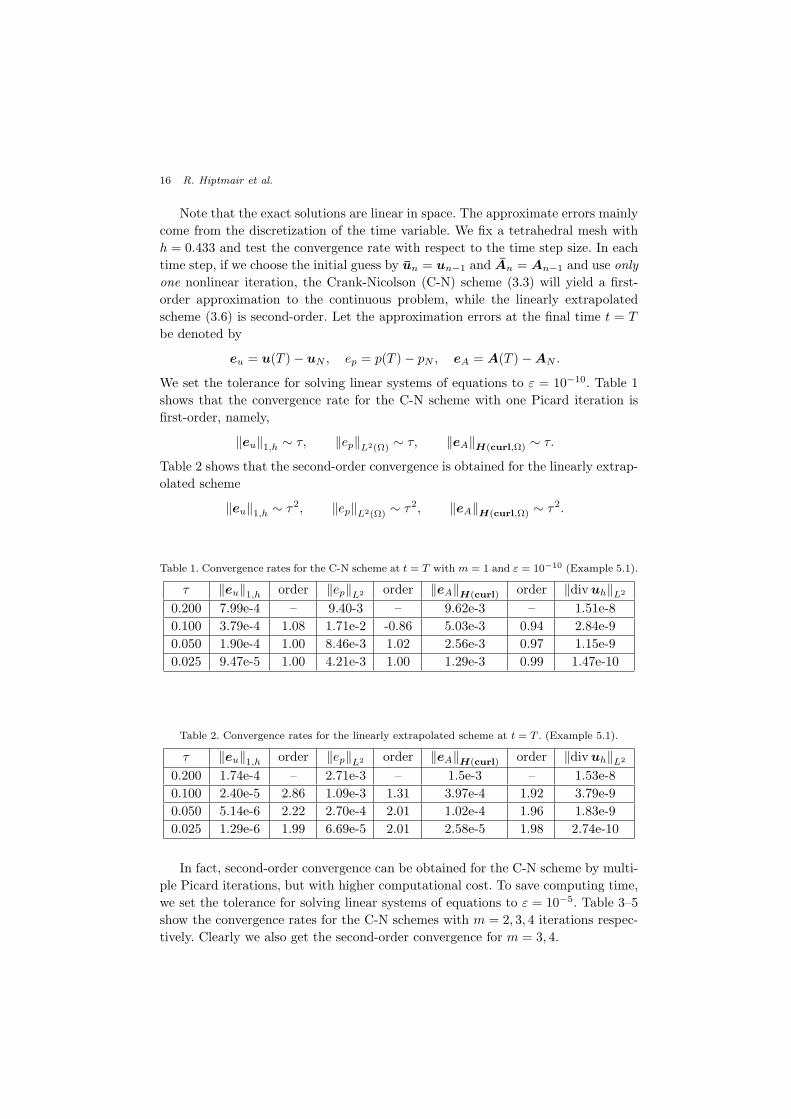
We set the tolerance for solving linear systems of equations to ε = 10−10. Table 1

shows that the convergence rate for the C-N scheme with one Picard iteration is

first-order, namely,

‖eu‖1,h ∼ τ, ‖ep‖L2(Ω) ∼ τ, ‖eA‖H(curl,Ω) ∼ τ.

Table 2 shows that the second-order convergence is obtained for the linearly extrap-

olated scheme

‖eu‖1,h ∼ τ2, ‖ep‖L2(Ω) ∼ τ2, ‖eA‖H(curl,Ω) ∼ τ2.

Table 1. Convergence rates for the C-N scheme at t = T with m = 1 and ε = 10−10 (Example 5.1).

τ ‖eu‖1,h order ‖ep‖L2 order ‖eA‖H(curl) order ‖divuh‖L2

0.200 7.99e-4 – 9.40-3 – 9.62e-3 – 1.51e-8

0.100 3.79e-4 1.08 1.71e-2 -0.86 5.03e-3 0.94 2.84e-9

0.050 1.90e-4 1.00 8.46e-3 1.02 2.56e-3 0.97 1.15e-9

0.025 9.47e-5 1.00 4.21e-3 1.00 1.29e-3 0.99 1.47e-10

Table 2. Convergence rates for the linearly extrapolated scheme at t = T . (Example 5.1).


0.200 1.74e-4 – 2.71e-3 – 1.5e-3 – 1.53e-8

0.100 2.40e-5 2.86 1.09e-3 1.31 3.97e-4 1.92 3.79e-9

0.050 5.14e-6 2.22 2.70e-4 2.01 1.02e-4 1.96 1.83e-9

0.025 1.29e-6 1.99 6.69e-5 2.01 2.58e-5 1.98 2.74e-10

In fact, second-order convergence can be obtained for the C-N scheme by multi-

ple Picard iterations, but with higher computational cost. To save computing time,

we set the tolerance for solving linear systems of equations to ε = 10−5. Table 3–5

show the convergence rates for the C-N schemes with m = 2, 3, 4 iterations respec-

tively. Clearly we also get the second-order convergence for m = 3, 4.


Table 3. Convergence rates for the C-N scheme at the final time with m = 2 (Example 5.1).


0.200 1.47e-4 – 8.60-4 – 8.20e-4 – 4.60e-7

0.100 5.54e-5 1.41 4.81e-4 0.84 2.79e-4 1.56 2.69e-7

0.050 1.86e-5 1.57 1.31e-4 1.88 9.25e-5 1.59 2.15e-8

0.025 5.71e-6 1.70 3.51e-5 1.90 3.02e-5 1.61 2.93e-9



0.200 7.63e-5 – 7.36e-4 – 7.49e-4 – 1.87e-8

0.100 1.78e-5 2.10 4.43e-4 0.78 2.07e-4 1.86 8.22e-9

0.050 4.44e-6 2.00 1.12e-4 1.98 5.33e-5 1.96 5.47e-10

0.025 1.13e-6 1.97 2.80e-5 2.00 1.35e-5 1.98 3.85e-11



0.200 7.60e-5 – 7.29e-4 – 7.44e-4 – 9.60e-10

0.100 1.77e-5 2.10 4.40e-4 0.73 2.05e-4 1.86 3.35e-10

0.050 4.40e-6 2.01 1.11e-4 1.99 5.29e-5 1.95 1.26e-11

0.025 1.11e-6 1.99 2.79e-5 1.99 1.34e-5 1.98 1.22e-11

To test the relative efficiency of the linear scheme to the nonlinear scheme, we

compare both the errors and the computing time for T = 10. We choose τ = 1/80,

ε = 10−10 for the linearly extrapolated scheme and τ = 1/40, ε = 10−5 for the

Crank-Nicolson scheme. We use m = 2, 3 Picard iterations for the nonlinear solver

respectively. Table 6 shows that the linearly extrapolated scheme is more efficient

for long-time simulations.

Table 6. The extrapolated scheme and the C-N scheme with m Picard iterations (T = 10).

Schemes τ Time (s) |eu|1,h ‖ep‖L2(Ω) ‖eA‖H(curl,Ω)

linear 1/80 2842 1.05e-6 1.92e-5 3.41e-5

C-N (m = 2) 1/40 2877 3.78e-6 6.44e-4 9.92e-5

C-N (m = 3) 1/40 4266 1.46e-6 2.62e-5 9.36e-5

Example 5.2. This example is to test the convergence rate for the linearly ex-

trapolated scheme where both the time step size and the mesh size are refined


simultaneously. The physical parameters are given by Re = Rm = κ = 1 and the

terminal time T = 0.2. The right-hand sides and the Dirichlet boundary conditions

are chosen so that the true solutions are given by

u = (sin t sin y, 0, 0) , p = x+ y + z − 1.5, A = (0, sin(t+ x), 0) .

We set the time step size by τ0 = 0.05 and the mesh size by h0 = 0.866 initially

and then bisect them successively. Table 7 shows the errors at the final time T .

Asymptotically, we find that

‖eu‖L2(Ω) ∼ O(τ2 + h2), ‖eA‖L2(Ω) ∼ O(τ2 + h2),

|eu|1,h ∼ O(τ2 + h), ‖eA‖H(curl,Ω) ∼ O(τ2 + h), ‖ep‖L2(Ω) ∼ O(τ2 + h).

Table 7. Optimal convergence in L2(Ω) norms (Example 5.2).

(τ, h) ‖eu‖L2 |eu|1,h ‖ep‖L2 ‖eA‖L2 ‖eA‖H(curl)

(τ0, h0) 7.6e-4 1.3e-2 1.8e-1 1.0e-2 7.5e-2

(τ0, h0)/2 1.9e-4 6.2e-3 8.9e-2 2.7e-3 3.7e-2

(τ0, h0)/4 4.9e-5 3.0e-3 4.4e-2 6.9e-4 1.8e-2

(τ0, h0)/8 1.3e-5 1.5e-3 2.2e-2 1.7e-4 9.1e-3

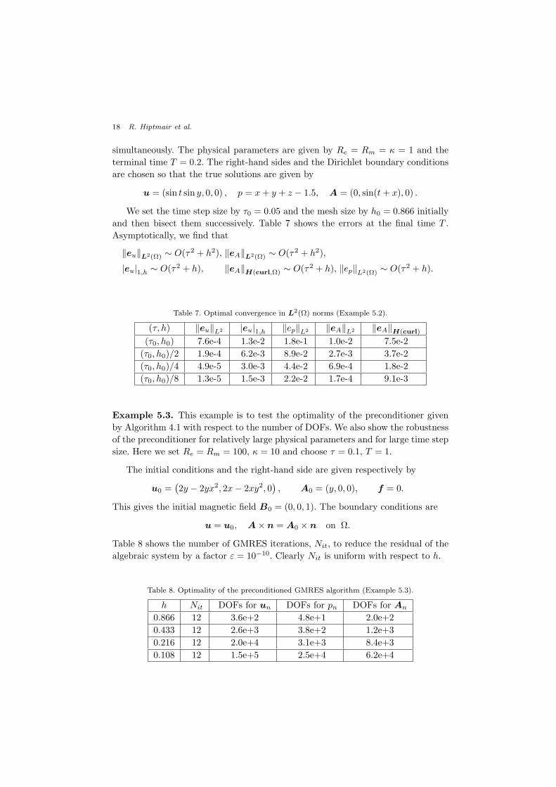
Example 5.3. This example is to test the optimality of the preconditioner given

by Algorithm 4.1 with respect to the number of DOFs. We also show the robustness

of the preconditioner for relatively large physical parameters and for large time step

size. Here we set Re = Rm = 100, κ = 10 and choose τ = 0.1, T = 1.

The initial conditions and the right-hand side are given respectively by

u0 =(

2y − 2yx2, 2x− 2xy2, 0)

, A0 = (y, 0, 0), f = 0.

This gives the initial magnetic field B0 = (0, 0, 1). The boundary conditions are

u = u0, A× n = A0 × n on Ω.

Table 8 shows the number of GMRES iterations, Nit, to reduce the residual of the

algebraic system by a factor ε = 10−10. Clearly Nit is uniform with respect to h.

Table 8. Optimality of the preconditioned GMRES algorithm (Example 5.3).

h Nit DOFs for un DOFs for pn DOFs for An

0.866 12 3.6e+2 4.8e+1 2.0e+2

0.433 12 2.6e+3 3.8e+2 1.2e+3

0.216 12 2.0e+4 3.1e+3 8.4e+3

0.108 12 1.5e+5 2.5e+4 6.2e+4


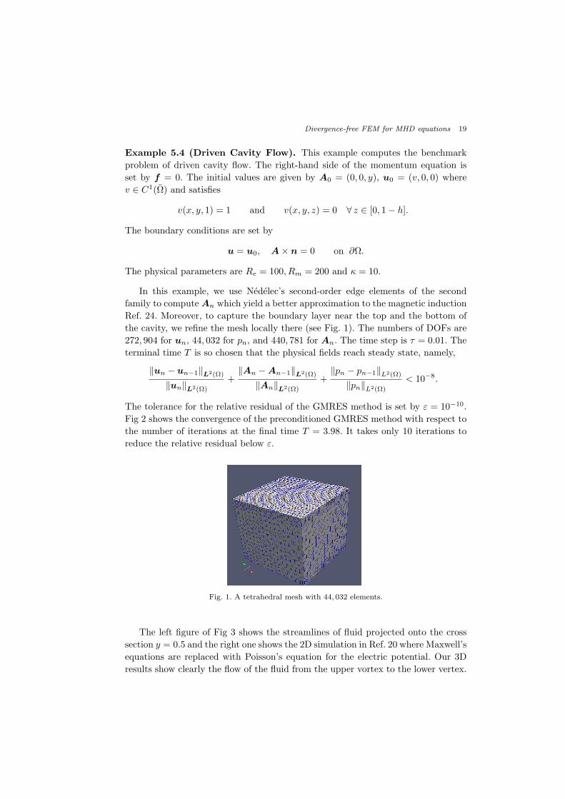
Example 5.4 (Driven Cavity Flow). This example computes the benchmark

problem of driven cavity flow. The right-hand side of the momentum equation is

set by f = 0. The initial values are given by A0 = (0, 0, y), u0 = (v, 0, 0) where

v ∈ C1(Ω) and satisfies

v(x, y, 1) = 1 and v(x, y, z) = 0 ∀ z ∈ [0, 1− h].

The boundary conditions are set by

u = u0, A× n = 0 on ∂Ω.

The physical parameters are Re = 100, Rm = 200 and κ = 10.

In this example, we use Nedelec’s second-order edge elements of the second

family to computeAn which yield a better approximation to the magnetic induction

Ref. 24. Moreover, to capture the boundary layer near the top and the bottom of

the cavity, we refine the mesh locally there (see Fig. 1). The numbers of DOFs are

272, 904 for un, 44, 032 for pn, and 440, 781 for An. The time step is τ = 0.01. The

terminal time T is so chosen that the physical fields reach steady state, namely,

‖un − un−1‖L2(Ω)

‖un‖L2(Ω)

+‖An −An−1‖L2(Ω)

‖An‖L2(Ω)

+‖pn − pn−1‖L2(Ω)

‖pn‖L2(Ω)

< 10−8.

The tolerance for the relative residual of the GMRES method is set by ε = 10−10.

Fig 2 shows the convergence of the preconditioned GMRES method with respect to

the number of iterations at the final time T = 3.98. It takes only 10 iterations to

reduce the relative residual below ε.

Fig. 1. A tetrahedral mesh with 44, 032 elements.

The left figure of Fig 3 shows the streamlines of fluid projected onto the cross

section y = 0.5 and the right one shows the 2D simulation in Ref. 20 where Maxwell’s

equations are replaced with Poisson’s equation for the electric potential. Our 3D

results show clearly the flow of the fluid from the upper vortex to the lower vertex.


Fig. 2. Number of GMRES iterations for reducing the relative residual below 10−10.

Fig. 3. Projection of the streamlines on the cross section y = 0.5

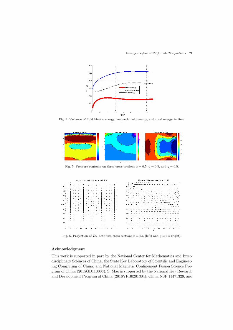
Fig. 4 shows the variation of the fluid kinetic energy Ekin, the magnetic field energy

Emag, and total energy E = Ekin + Emag with respect to time, where

Ekin =1

2‖un‖

2L2(Ω) , Emag =

κ

2Rm‖curlAn‖

2L2(Ω) .

When the fluid tends to be steady, the total energy and the two portions of the

total energy become invariant in time.

Fig. 5 shows the distribution of the kinetic pressure on three cross sections

x = 0.5, y = 0.5, and z = 0.5 respectively. In the middle figure, since the flow is

driven from left to right, it generates high pressure regions near the left and the

right upper corners. Fig. 6 shows magnetic lines of Bn on the cross section x = 0.5

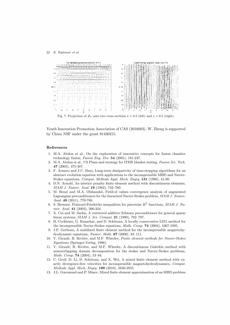
and the cross section y = 0.5 respectively. Fig. 7 shows the eddy current density Jn

on the cross section x = 0.5 and the cross section z = 0.5 respectively. They tells

us how the fluid influences the electromagnetic fields.


Fig. 4. Variance of fluid kinetic energy, magnetic field energy, and total energy in time.

Fig. 5. Pressure contours on three cross sections x = 0.5, y = 0.5, and y = 0.5.

Fig. 6. Projection of Bn onto two cross sections x = 0.5 (left) and y = 0.5 (right).

Acknowledgment

This work is supported in part by the National Center for Mathematics and Inter-

disciplinary Sciences of China, the State Key Laboratory of Scientific and Engineer-

ing Computing of China, and National Magnetic Confinement Fusion Science Pro-

gram of China (2015GB110003). S. Mao is supported by the National Key Research

and Development Program of China (2016YFB0201304), China NSF 11471329, and


Fig. 7. Projection of Jn onto two cross sections x = 0.5 (left) and z = 0.5 (right).

Youth Innovation Promotion Association of CAS (2016003). W. Zheng is supported

by China NSF under the grant 91430215.

References

1. M.A. Abdou et al., On the exploration of innovative concepts for fusion chambertechnology fusion, Fusion Eng. Des. 54 (2001), 181-247.

2. M.A. Abdou et al., US Plans and strategy for ITER blanket testing, Fusion Sci. Tech.

47 (2005), 475-487.3. F. Armero and J.C. Simo, Long-term dissipativity of time-stepping algorithms for an

abstract evolution equation with applications to the incompressible MHD and Navier-Stokes equations, Comput. Methods Appl. Mech. Engrg. 131 (1996), 41-90.

4. D.N. Arnold, An interior penalty finite element method with discontinuous elements,SIAM J. Numer. Anal. 19 (1982), 742–760.

5. M. Benzi and M.A. Olshanskii, Field-of values convergence analysis of augmentedLagrangian preconditioners for the linearized Navier-Stokes problem, SIAM J. Numer.

Anal. 49 (2011), 770-788.6. S. Brenner, Poincare-Friedrichs inequalities for piecewise H

1 functions, SIAM J. Nu-

mer. Anal. 41 (2003), 306-324.7. X. Cai and M. Sarkis, A restricted additive Schwarz preconditioner for general sparse

linear systems, SIAM J. Sci. Comput. 21 (1999), 792–797.8. B. Cockburn, G. Kanschat, and D. Schotzau, A locally conservative LDG method for

the incompressible Navier-Stokes equations, Math. Comp. 74 (2004), 1067-1095.9. J.F. Gerbeau, A stabilized finite element method for the incompressible magnetohy-

drodynamic equations, Numer. Math. 87 (2000), 83–111.10. V. Girault, B. Riviere, and M.F. Wheeler, Finite element methods for Navier-Stokes

Equations (Springer-Verlag, 1986).11. V. Girault, B. Riviere, and M.F. Wheeler, A discontinuous Galerkin method with

nonoverlapping domain decomposition for the stokes and Navier-Stokes problems,Math. Comp. 74 (2004), 53–84.

12. C. Greif, D. Li, D. Schotzau, and X. Wei, A mixed finite element method with ex-actly divergence-free velocities for incompressible magnetohydrodynamics, Comput.

Methods Appl. Mech. Engrg. 199 (2010), 2840-2855.13. J.L. Guermond and P. Minev, Mixed finite element approximation of an MHD problem


involving conducting and insulating regions: the 3D case, Numer. Meth. Part. Diff.

Eqns. 19 (2003), 709–731.14. M.D. Gunzburger, A.J. Meir, and J.S. Peterson, On the existence and uniqueness and

finite element approximation of solutions of the equations of stationary incompressiblemagnetohydrodynamics, Math. Comp. 56 (1991), 523–563.

15. P. Hansbo and M.G. Larson, Discontinuous Galerkin methods for incompressible andnearly incompressible elasticity by Nitsche’s method, Comput. Methods Appl. Mech.

Engrg. 191 (2002), 1895–1908.16. R. Hiptmair, Finite elements in computational electromagnetism, Acta Numerica 11

(2002), 237–339.17. R. Hiptmair and J. Xu, Nodal auxiliary space preconditioning in H(curl) and H(div)

spaces, SIAM J. Numer. Anal. 45 (2007), 2483–2509.18. K. Hu, Y. Ma, and J. Xu, Stable finite element methods preserving ∇·B = 0 exactly

for MHD models, Numer. Math. 135 (2017), 371-396.19. Y. Ma, K. Hu, X. Hu, and J. Xu, Robust preconditioners for incompressible MHD

models, J. Comput. Phys. 316 (2016), 721–746.20. L. Marioni, F. Bay, and E. Hachem, Numerical stability analysis and flow simulation

of lid-driven cavity subjected to high magnetic field, Phys. Fluids 28 (2016), 057102.21. K.A. Mardal and R. Winther, Preconditioning discretizations of systmes of partial

differential equations, Numer Linear Algebra Appl. 18 (2011), 1–40.22. P. Monk, Finite Element Methods for Maxwells Equations (Oxford University Press,

2003).23. R. Moreau, Magnetohydrodynamics (Kluwer Academic Publishers, 1990).24. J.C. Nedelec, A new family of mixed finite elements in R3, Numer. Math. 50 (1986),

57–81.25. M.-J. Ni, R. Munipalli, P. Huang, N.B. Morley, M.A. Abdou, A current density con-

servative scheme for incompressible MHD flows at a low magnetic Reynolds number.Part I. On a rectangular collocated grid system, J. Comp. Phys. 227 (2007), 174–204.

26. M.-J. Ni, R. Munipalli, P. Huang, N.B. Morley, M.A. Abdou, A current density con-servative scheme for incompressible MHD flows at a low magnetic Reynolds number.Part II: On an arbitrary collocated mesh, J. Comp. Phys. 227 (2007), 205–228.

27. D. Schotzau, Mixed finite element methods for stationary incompressible magneto-hydrodynamics, Numer. Math. 96 (2004), 771–800.

28. J. Xin, W. Cai, and N. Guo, On the construction of well-conditioned hierarchical basesfor H(div)-conforming Rn simplicial elements, Commun. Comput. Phys. 14 (2013),621–638.

29. S.J. Xu, N.M. Zhang, and M.J. Ni, Influence of flow channel insert with pressureequalization opeing on MHD flows in a rectangular duct, Fusion Eng. Des. 88 (2013),271–275.

30. Y. Zhang, Y. Hou, and L. Shan, Numerical analysis of the Crank-Nicolson extrapola-tion time discrete scheme for magnetohydrodynamics flows, Numer. Methods Partial

Differential Equations 31 (2015), 2169–2208.31. J. Zhang and M.J. Ni, A consistent and conservative scheme for MHD flows with

complex boundaries on an unstructured Cartesian adaptive system, J. Comp. Phys.

256 (2014) 520–542.32. L. Zhang, A parallel algorithm for adaptive local refinement of tetrahedral

meshes using bisection, Numer. Math.: Theor. Method Appl. 2 (2009), 65–89.(http://lsec.cc.ac.cn/phg)

A fully divergence-free finite element method for magneto-hydrodynamic ... A fully divergence-free...

Documents

Transcript of A fully divergence-free finite element method for magneto-hydrodynamic ... A fully divergence-free...