a force-sensing device for assistance in soft-tissue ... · Lord William Thomson Kelvin (1824-1907)...
129
THÈSE N O 3398 (2005) ÉCOLE POLYTECHNIQUE FÉDÉRALE DE LAUSANNE PRÉSENTÉE À LA FACULTÉ SCIENCES ET TECHNIQUES DE L'INGÉNIEUR Institut de production et robotique SECTION DE MICROTECHNIQUE POUR L'OBTENTION DU GRADE DE DOCTEUR ÈS SCIENCES PAR ingénieur physicien diplômé EPF de nationalité suisse et originaire de Portalban (FR) acceptée sur proposition du jury: Lausanne, EPFL 2005 Prof. H. Bleuler, directeur de thèse Dr L. Dürselen, rapporteur Prof. L. Nolte, rapporteur Prof. P. Ryser, rapporteur A FORCE-SENSING DEVICE FOR ASSISTANCE IN SOFT-TISSUE BALANCING DURING KNEE ARTHROPLASTY Denis CROTTET
Transcript of a force-sensing device for assistance in soft-tissue ... · Lord William Thomson Kelvin (1824-1907)...

THÈSE NO 3398 (2005)
ÉCOLE POLYTECHNIQUE FÉDÉRALE DE LAUSANNE
PRÉSENTÉE à LA FACULTÉ SCIENCES ET TECHNIQUES DE L'INGÉNIEUR
Institut de production et robotique
SECTION DE MICROTECHNIQUE
POUR L'OBTENTION DU GRADE DE DOCTEUR ÈS SCIENCES
PAR
ingénieur physicien diplômé EPFde nationalité suisse et originaire de Portalban (FR)
acceptée sur proposition du jury:
Lausanne, EPFL2005
Prof. H. Bleuler, directeur de thèseDr L. Dürselen, rapporteurProf. L. Nolte, rapporteurProf. P. Ryser, rapporteur
a force-sensing device for assistance in soft-tissue balancing during knee arthroplasty
Denis CROTTET


.
“If you cannot measure it, you cannot improve it.”Lord William Thomson Kelvin (1824-1907)


Acknowledgements
I would like to thank first Prof. Hannes Bleuler and Prof. Lutz-P. Nolte,my supervisors, who gave me the opportunity to realize this interesting workand who guided me throughout my doctoral thesis. My very warm thanksalso go to my co-advisers, Dr. Ion P. Pappas and Dr. Jens Kowal, for theircontinuous support and their ideas, as well as their enthusiasm, which largelycontributed to the achievements presented herein.
For the helpful advice during the design phase and for the deposition of thesensors, I am very grateful to Dr. Thomas Maeder and his team members,Giancarlo Corradini, Caroline Jacq and Matthias Garcin, from the Labora-toire de Production Microtechnique, EPFL.
I heartily thank Dr. Sven Sarfert from the Department of OrthopaedicSurgery of the Inselspital, Bern, for his clinical support during the in-vitrostudies and in-vivo trials. I particularly appreciated his availability, a rarequality by surgeons.
I also thank very much Dr. Lutz Dürselen from the Institute of OrthopaedicResearch and Biomechanics, University of Ulm, Germany, for his collabora-tion and support during the in-vitro study.
My thanks go of course to all my colleagues who contributed to add to theprofessional experience a unique human experience. The large variety of ori-gins represented at the institute allowed me to discover different cultures andwonderful people. Among these, I would like to address special thanks to theso-called "French Connection" (even if a minority of members were French),Heinz Waelti, Ségolène Tarte, Gisèle Douta, Serge Sagbo, Viton Vitanis, fortheir friendliness, for the funny lunch breaks, for the moral support and forall the nice souvenirs. To the technicians, Philippe Gédet, Thomas Beutler,Ladina Ettinger and to the machine shop team, Urs Rohrer, Erland Mühleim,Thomas Gerber, Remo Walther, Sebastian Marti, for their friendly, effective
III
IV
and high-quality assistance in producing mechanical parts, setting up ex-perimental benches or testing materials. To Manuela Kunz, for her helpfuladvice and ideas. To Anne Polikeit and Philippe Büchler for their technicalsupport in numerical simulations. To Haydar Talib and Paul Thistlethwaite,who accepted the tedious task of proof reading the present thesis. To thetwo sweetest secretaries (in literal and figurative meanings), Esther Gna-horé and Annelies Neuenschawander, for their good mood and their boostingchocolates. And finally, to my former and current group colleagues, JonasChapuis, Christian Sigrist, Jubei Liu, Puja Malik, Blake Borgeson, ElenaDe Momi, Jaime Garcia, Brenton Ebert, Mario Löffel, Michaël Bläuer, LarsEbert, Marc Puls, Tobias Rudolph, Anna Martina Bröhan, who did theirbest to transform the routine into a funny daily life.
Finally I am very grateful to all those, outside the working sphere, whoaccompanied me along these four years: my close friends, my family, andmore particularly my wife Martine who always encouraged me by findingcomforting words in the critical moments and by lovingly congratulating mein times of success.
Contents
Abstract 1
Version abrégée 3
1 Introduction 5
2 Total knee arthroplasty 92.1 Anatomy of the knee . . . . . . . . . . . . . . . . . . . . . . . 92.2 Total knee arthroplasty . . . . . . . . . . . . . . . . . . . . . . 112.3 Computer assisted knee surgery . . . . . . . . . . . . . . . . . 152.4 A force-sensing device for TKA . . . . . . . . . . . . . . . . . 15
3 Force-sensing device design 193.1 Simplified biomechanical model . . . . . . . . . . . . . . . . . 193.2 Techniques to measure forces . . . . . . . . . . . . . . . . . . . 20
3.2.1 Capacitive sensors . . . . . . . . . . . . . . . . . . . . 213.2.2 Magnetic, inductive sensors . . . . . . . . . . . . . . . 223.2.3 Strain gauges . . . . . . . . . . . . . . . . . . . . . . . 233.2.4 Choice of the measurement principle . . . . . . . . . . 24
3.3 Definition, evaluation of possible designs . . . . . . . . . . . . 253.3.1 Design I: opposed bending beams . . . . . . . . . . . . 263.3.2 Design II: open load cell . . . . . . . . . . . . . . . . . 293.3.3 Design III: integrated bridges . . . . . . . . . . . . . . 31
4 Thick-film piezoresistive sensors 434.1 Piezoresistive effect . . . . . . . . . . . . . . . . . . . . . . . . 434.2 Thick-film technology . . . . . . . . . . . . . . . . . . . . . . . 444.3 Mechanical properties . . . . . . . . . . . . . . . . . . . . . . . 444.4 Custom low-temperature dielectric . . . . . . . . . . . . . . . 46
V

VI CONTENTS
5 Calibration and intrinsic accuracy 475.1 Calibration method . . . . . . . . . . . . . . . . . . . . . . . . 475.2 Intrinsic accuracy . . . . . . . . . . . . . . . . . . . . . . . . . 485.3 Accuracy in the extended sensitive area . . . . . . . . . . . . . 535.4 Accuracy with spacers . . . . . . . . . . . . . . . . . . . . . . 535.5 Calibration and autoclave sterilization . . . . . . . . . . . . . 535.6 Plastic deformation . . . . . . . . . . . . . . . . . . . . . . . . 56
6 In-vitro study 596.1 Control experiment with a plastic model . . . . . . . . . . . . 596.2 In-vitro trials . . . . . . . . . . . . . . . . . . . . . . . . . . . 616.3 In-situ evaluation . . . . . . . . . . . . . . . . . . . . . . . . . 63
6.3.1 Method . . . . . . . . . . . . . . . . . . . . . . . . . . 636.3.2 Results . . . . . . . . . . . . . . . . . . . . . . . . . . . 686.3.3 Discussion . . . . . . . . . . . . . . . . . . . . . . . . . 75
7 Clinical trials 797.1 Safety requirements . . . . . . . . . . . . . . . . . . . . . . . . 797.2 Standard approach vs force-sensing device . . . . . . . . . . . 82
8 Unicompartmental knee arthroplasty 858.1 Surgical procedure . . . . . . . . . . . . . . . . . . . . . . . . 858.2 Soft-tissue balancing assistance for UKA . . . . . . . . . . . . 87
8.2.1 Concept . . . . . . . . . . . . . . . . . . . . . . . . . . 878.2.2 In-vitro feasibility study . . . . . . . . . . . . . . . . . 89
9 Conclusion and perspectives 91
A Some basics of solid mechanics 95A.1 Elastic deformation . . . . . . . . . . . . . . . . . . . . . . . . 95A.2 Stresses in beams . . . . . . . . . . . . . . . . . . . . . . . . . 99
B Contact pressure and stresses 103B.1 Hertzian theory . . . . . . . . . . . . . . . . . . . . . . . . . . 103B.2 Distortion-energy criterion . . . . . . . . . . . . . . . . . . . . 106B.3 Conclusion . . . . . . . . . . . . . . . . . . . . . . . . . . . . . 108
Bibliography 111
Curriculum Vitae 119
Abstract
Nowadays, the large majority of the instrumentation for orthopaedic surgeryconsists of mechanical tools with varying degrees of complexity. To increasethe accuracy and the safety of orthopaedic interventions, sensors and com-puters were recently introduced in the operating room. Computer AssistedOrthopaedic Surgery (CAOS) uses a navigation system that tracks the move-ments of surgical instruments in real-time and displays their exact locationin relation to the operative area. Such technology improved the quality oforthopaedic arthroplasties, but it is still limited to the measurement of kine-matic parameters such as axial alignments, position and angle measurements.In Total Knee Arthroplasty (TKA), the ligament balance, which is crucial forthe stability and lifetime of implants, is currently only qualitatively assessed.The goal of this thesis was therefore to demonstrate the importance of intra-operative measurement of musculoskeletal forces through the development ofa force-sensing device designed to improve the ligament balancing procedureduring TKA.
Three possible device designs were proposed and evaluated using finite ele-ment analysis in an iterative optimization process. The final design consistsof two sensitive plates, one for each condyle, a tibial base plate and a set ofspacers to adapt the device thickness to the patient-specific tibiofemoral gaps.Each sensitive plate is equipped with three deformable bridges instrumentedwith thick-film piezoresistive sensors, which allow accurate measurements ofthe amplitude and location of the tibiofemoral contact forces. The net varus-valgus moment is then computed to characterize the ligament imbalance.
Laboratory experiments showed that the device has appropriate accuracyand dynamic range for the intended application. The first experimental tri-als on a plastic knee joint model and on a cadaver specimen demonstratedthe proper in-situ functioning of the device. The performance and surgicaladvantages of the device were then evaluated in an in-vitro study includingfour different experiments: 1) Six knee joints were axially loaded. Com-
1
2 ABSTRACT
paring applied and measured compressive forces demonstrated the accuracyand reliability of in-situ measurements. 2) To estimate the importance ofkeeping the patella in its anatomical place during imbalance assessment, theeffect of patellar eversion on the mediolateral distribution of tibiofemoralcontact forces was measured. One fourth of the patellar load was shifted tothe lateral compartment. 3) Assessment of knee stability based on condylecontact forces or varus-valgus moments were compared to the current sur-gical method (difference of varus-valgus loads causing condyle lift-off). Theforce-based assessment found to be equivalent to the surgical method whilethe moment-based technique, which is considered optimal, showed a ten-dency of lateral imbalance. 4) Finally the effect of minor and major medialcollateral ligament releases was biomechanically quantified. Large variationamong specimens reflected the difficulty of ligament release and the need forintraoperative force monitoring.
Two clinical trials were carried out to evaluate the device performance in asurgical environment. After the tibial cut, the medial and lateral tibiofemoralgaps ensuring the knee stability were determined from the device measure-ments and compared to the femoral cuts performed on the basis of standardinstrumentation. The agreement between the two approaches was generallygood. The only significant difference was measured on the first patient at90◦ flexion. At this point, the surgeon also estimated that the knee was notoptimally balanced, thus demonstrating the consistency between his percep-tion and the device measurements.
In conclusion, the proposed force-sensing device for assistance in ligamentbalancing during TKA provides accurate, reliable and useful measurements.In addition to the precise imbalance assessment based on the measurementof forces and moments, important clinical advantages, such as the possibil-ity to keep the patella in its anatomical place during the measurement orthe real-time force monitoring during the delicate phase of ligament release,were demonstrated. The encouraging results of the in-vivo trial proved theusability of the device in a surgical environment and opens the way for largerclinical studies. The developed device has thus potential to improve theligament balancing procedure, the consistency of surgery and the lifetimeof TKA, illustrating thereby the clinical benefit of measuring forces duringorthopaedic surgeries.

Version abrégée
De nos jours, la majeure partie de l’instrumentation pour la chirurgie or-thopédique est constituée d’outils mécaniques plus ou moins complexes. Afind’améliorer la précision et la sécurité de ces interventions, senseurs et ordi-nateurs ont récemment fait leur apparition en salle d’opération. La chirurgieorthopédique assistée par ordinateur utilise un système de navigation quisuit en temps réel les mouvements des instruments chirurgicaux et afficheleur position exacte par rapport à la zone opérée. Une telle technologie aamélioré la qualité des interventions mais reste malheureusement limitée à lamesure de paramètres cinématiques tels que axes, angles ou positions. Lorsd’Arthroplastie Totale du Genou (ATG), l’équilibre ligamentaire, qui est cru-cial pour la stabilité et la durée de vie des implants, est actuellement évaluéuniquement qualitativement à l’aide de manipulations ou d’outils basiques.Le but de cette thèse était donc de montrer l’importance de la mesure in-traopératoire des forces musculosquelettiques au travers du développementd’un capteur de force conçu pour améliorer la procédure d’équilibrage liga-mentaire lors d’ATG.
Trois designs possibles ont été proposés et évalués en utilisant la méthodedes éléments finis au cours d’un processus itératif d’optimisation. Le de-sign final comprend deux plaques sensibles, une pour chaque condyle, uneplaque de base tibiale et un set d’écarteurs pour adapter l’épaisseur du cap-teur à l’espace tibiofémoral du patient. Chaque plaque sensible comprendtrois ponts déformables équippés de senseurs piézorésistifs qui permettentde mesurer précisément l’amplitude et la position des forces de contact descondyles fémoraux. Le moment résultant dans les directions varus et valgusest ensuite calculé pour caractériser l’équilibre ligamentaire.
Les expériences en laboratoire ont montré que le capteur a une précision etune plage de mesure appropriées pour l’application envisagée. Les premiersessais sur un modèle en plastique et sur un spécimen cadavérique ont dé-montré le bon fonctionnement du capteur in-situ. Les performances et les
3
4 VERSION ABRÉGÉE
avantages chirurgicaux du capteur ont ensuite été évalués au travers d’uneétude in-vitro comprenant quatre expériences différentes: 1) Six genoux ontété chargés axialement. La comparaison entre les forces de compression ap-pliquées et mesurées a démontré la précision et la fiabilité des mesures in-situ.2) Afin d’estimer l’importance de garder la rotule à sa place anatomiquedurant l’évaluation du déséquilibre, l’effet d’une éversion rotulienne sur ladistribution mediolatérale des forces de contact a été mesuré : un quart de laforce rotulienne est déplacé sur le compartiment latéral. 3) L’évaluation de lastabilité du genou basée sur les forces de contact des condyles ou sur leur mo-ment a été comparée à la méthode chirurgicale actuelle (différence de poidsvarus ou valgus créant un décollement d’un condyle). L’évaluation baséesur les forces fut équivalente à l’approche chirurgicale alors que celle baséesur les moments, considérée comme optimale, a montré une tendance à undéséquilibre latéral. 4) Finalement, l’effet de relâches ligamentaires mineuresou majeures du ligament collatéral médial a été quantifié biomécaniquement.L’importante variation parmi les spécimens a révélé la difficulté de la relâcheligamentaire et le besoin d’un monitoring intraopératoire des forces.
Deux essais cliniques ont été effectués pour évaluer le fonctionnement ducapteur dans un environnement chirurgical. Après la coupe tibiale, les es-paces tibiofémoraux médial et latéral assurant la stabilité du genou ont étédéterminés selon les mesures du capteur et comparés aux coupes fémorales ef-fectuées sur la base de l’instrumentation habituelle. L’accord entre les deuxapproches était généralement bon. La seule différence significative a étémesurée sur le premier patient à 90◦ de flexion. A ce moment, le chirurgienestimait également que le genou n’était pas équilibré de façon optimale, dé-montrant ainsi la cohérence entre sa perception et les mesures du capteur.
En conclusion, le capteur de force proposé pour l’assistance durant l’équili-brage ligamentaire lors d’ATG fournit des mesures précises, fiables et utiles.En plus d’une évaluation quantitative du déséquilibre basée sur la mesure deforces et de moments, des avantages cliniques importants ont été démontrés,comme par exemple la possibilité de garder la rotule à sa place anatomiqueou le monitoring des forces de contact lors de la relâche ligamentaire. Lesrésultats encourageant de l’essai clinique ont prouvé que le capteur fonctionneparfaitement dans un environnement chirurgical, ouvrant ainsi la voie à deplus larges études cliniques. Le capteur développé a donc montré un potentielpour améliorer la procédure d’équilibrage ligamentaire, la consistance de lachirurgie et la durée de vie d’une ATG, illustrant ainsi le bénéfice de mesuresde forces lors d’opérations orthopédiques.

Chapter 1
Introduction
Orthopaedic surgery, which is the branch of surgery concerned with injuriesand disorders of the musculoskeletal system, is an ancient discipline. Arche-ological traces, such as a prosthesis for a big toe after a healed amputationfound on a mummy (circa 1065-650 BC) [1] or the guidelines and reportsof surgical cases in the Edwin Smith papyrus (circa 1700 BC) [2], were dis-covered in Egypt. Other ancient civilizations, such as Greeks or Romans,reported orthopaedic knowledge as well. Various volumes of the importantGreek text Corpus Hippocrates (circa 430-330 BC) from the name of thefamous father of medicine had relevance to orthopaedics. For example, anentire volume is dedicated to joints, where dislocation of the shoulder, knee,hip and elbow joint was described together with the various methods usedfor reduction. It was nevertheless not before the l2th century that Europebegan to awake gradually from its dark ages. Universities and hospitals werebeing established, human dissection resumed and the great Greek texts werebeing translated. However, until the l6th century, all developments remainedwithin the shadow cast by Hippocrates. Some of the new techniques intro-duced at that time were the use of a tourniquet and the ligature for largevessels for amputations or the development of artificial limbs using iron orwood. Modern orthopaedics started only in the early 1900’s with the discov-ery of the X-ray and with the fact that orthopaedics became a specialty inits own. From that point in time the tools for diagnosis, surgical techniquesand instrumentation had been continuously improved to the end of obtainingpredictable and satisfying outcome of orthopaedic interventions.
Nowadays, the large majority of the instrumentation for orthopaedic surgeryconsists in more or less complex mechanical tools. Chisels, saws, drillersrequired to correct or repair bony structure are used in combination withmechanical ancillaries, providing the surgeon with geometrical parameters
5
6 CHAPTER 1. INTRODUCTION
such as bone axes, morphologic angulations or distances between bones. Toincrease the accuracy and the safety of orthopaedic interventions, sensorsand computers were recently introduced in the operating room. ComputerAssisted Orthopaedic Surgery (CAOS) uses a navigation system that tracksin real-time the movements of the surgical instruments and displays theirexact location in relation to the operative area [3]. Such technology enablesmore precise placement of implants and safer delicate surgical actions, suchas the insertion of a pedicle screw in a vertebral body. With the arrivalof CAOS systems, surgical instrumentation reached an important turningpoint and is now experiencing the same natural evolution as the automotiveindustry during these past decades. Sensors, calculators, automatic controlor management are common features in cars nowadays. An Audi A8 for in-stance contains 45 calculators in its standard version and more than 75 withfull options. Even though refractories claimed that this proliferation of elec-tronic components in cars would just increase the risk of break-downs, a largenumber of new technologies such as airbags, Anti-lock Brake System (ABS),automatic gear change or power-assisted steering have significantly improvedthe safety and comfort of the end users. According to the first short-termclinical studies, the same benefits can be hoped in the CAOS systems.
However, current navigation systems, although competitive, are mainly lim-ited to the control of geometrical parameters. Stresses in soft-tissue or forcesapplied by the surgeon are important biomechanical parameters which usu-ally remain unknown. Measurement of forces with smart instrumentationcan therefore improve the quality of orthopaedic surgery in three differentways:
1. Detection of possible damage of healthy tissues. When the surgeonhas no direct access to the operation site, as during minimally inva-sive surgery, manual guidance of the tools is difficult. Integrating forcesensors in the surgical tools can help to detect undesired contact orpenetration in healthy tissue. For example, an arthroscope equippedwith force sensors can detect contact between its tip and the surround-ing tissues [4], thus preventing possible damage of the cartilage. Asecond example of application is a mechatronic tool for drilling in theosteosynthesis of long bones [5]. In that case, the measurement of thevariation of the thrust force experienced by the driller allows determin-ing if the drill bit is in cancellous or cortical bone. When a bone isdrilled across, the time of incipient breakthrough on the second cor-tical wall can thus be detected and the hole completed with minimalprotrusion of the drill bit from the bone.

7
2. Force monitoring of surgical actions. While being corrected, cut, rasped,or reshaped, bones experience relatively high stresses. Applying exces-sive forces on the bony structure can create irreversible damage or givesuboptimal outcomes. Instrumenting orthopaedic tools with force sen-sors can provide useful real-time force-feedback and thereby ensure safeand optimal surgical actions. In the case of correction of scoliosis forexample, the realignment of the spine is realized by implanting a rodscrewed in the misaligned vertebral bodies. In addition to the axialpull-out strength, the screws are loaded with a force component per-pendicular to the screw axis, which may weaken the bone around thehead and lower the pull-out force. A high correction force thereforeincreases the risk of screw pull-out. Instrumented forceps that measuretensile forces in the different segment of the rod can thus be used tomaintain constant axial forces in the rod and reduce the transverse forceon the vertebral screws [6]. A second example of application could berasps instrumented with force sensors for the preparation of the femoralcavity in hip arthroplasty. Since there is a direct correlation betweenthe rasping force and the bone density, the measurement of the latterallows the determination of the optimal rasping force. This optimumcan then be intraoperatively guaranteed thanks to a monitoring basedon the smart rasp measurements, thus avoiding excessive forces thatmay damage the femur.
3. Assistance for optimal adjustment of the soft-tissue forces in joint arthro-plasty. Joint arthroplasty is used to treat severe arthrosis and bonedeformities. To achieve a satisfying stability and lifetime of the pros-thetic joint, the alignment of the bones and the forces experienced bythe surrounding soft-tissue must be optimally corrected at the time ofthe surgery. The intraoperative use of instrumented trial implants orspecific force-sensing devices could provide valuable measurements toassist the surgeon in optimally balancing the soft-tissue tensions. Twodifferent applications can be thought for the two most performed jointarthroplasties: an instrumented telescopic neck for Total Hip Arthro-plasty (THA) and a force-sensing device for Total Knee Arthroplasty(TKA). One serious problem after THA is dislocation, which is at-tributed to component malpositioning, soft-tissue imbalance and im-pingement. An advanced trial implant could allow the medializationand lateralization of the prosthesis and the measurement of the resul-tant hip force by means of a telescopic neck instrumented with force-sensors. The surrounding soft-tissue such as muscles, fascia, could bemore or less stressed by adjusting the length of the neck until the op-

8 CHAPTER 1. INTRODUCTION
timal resultant hip force is obtained. This procedure may then lead tothe proper choice of the prosthetic components, reducing the rate ofdislocations in THA. In the knee, the stability of the joint is realized bya complex ligament structure. At the time of arthroplasty, this stabilitymust be reevaluated and, if necessary, corrected to ensure a successfuloutcome. A force-sensing device that can precisely measure intraop-erative mediolateral imbalance of the compressive forces of the kneejoint could assist the surgeon in this delicate phase of ligament balanc-ing. This would guarantee an optimal distribution of the compressiveforces,leading to an increased lifetime of the prosthetic implants.
The goal of the present work is therefore to demonstrate through an appli-cation the importance and benefit of advanced orthopaedic instrumentationproviding quantitative knowledge of intraoperative forces. A force-sensingdevice for improved ligament balancing procedure in knee arthroplasty hasbeen developed and tested. Chapter 2 presents general aspects of the kneejoint anatomy and of TKA as well as the specifications of such force-sensingdevice. The different conceived designs are explained and studied in chapter3, while the selected sensor technology is described in chapter 4. The cal-ibration method and the evaluation of the intrinsic accuracy of the deviceis exposed in chapter 5. The result of the in-situ evaluation of the devicedesign as well as biomechanical investigations about the effect of ligamentreleasing can be found in chapter 6. Finally, the possible extension of the de-veloped device to unicompartmental knee arthroplasty is discussed in chapter8, before concluding this thesis in chapter 9.
Chapter 2
Total knee arthroplasty
2.1 Anatomy of the knee
The knee is the largest and most complex joint in the human body and com-bines two major joint mechanisms. On one hand, it fulfills the requirementsof stability, which allows the transmission of large forces. For example, theknee bears three to four times the body weight during stair climbing. Onthe other hand, it provides a high degree of flexibility with a range of mo-tion of up to 140◦ in flexion. The combination of these two functionalitiesis only possible by a perfect interplay between all the components of the knee.
The knee is indeed a two-joint structure composed of the tibiofemoral andpatellofemoral joints [7]. The tibiofemoral joint connects the two longestbones in the human body, namely the femur and the tibia (Fig.2.1). Thejoint-constructing bone segments are overlaid by cartilage, which protectsthe bones and ensures free sliding. The absence of bony guidance is compen-sated by a complex structure of ligaments, which are dense parallel-fiberedcollagenous tissue. Two collateral ligaments (medial and lateral) limit themediolateral translation from the tibia with respect to the femur and theso-called abduction-adduction rotation movements. Two cruciate ligaments(anterior and posterior) restrict the translation of the tibia to the femur inanterior and posterior directions. In the tibiofemoral gap are found the lat-eral and medial menisci, which compensate the bony incongruency and allowcompressive forces to be distributed over the entire area of the tibial plateau,thus minimizing the contact stresses.
The patellofemoral joint (Fig.2.2) consists of the femur and the patella, whichis a flat bone placed as a cap to the knee. The patella is held by the patellar
9

10 CHAPTER 2. TOTAL KNEE ARTHROPLASTY
Figure 2.1: Anatomy of the knee(picture adapted from the anatomy atlas of ADAM, Atlanta, USA)
tendon on the tibial side and by the quadriceps, the most effective activeknee stabilizers, on the femoral side. The patellofemoral joint supports theextension of the knee and works as a sagittal stabilizer. The patella is also aprotection for the knee in the frontal plane.
Quadriceps
Patella
Patellar tendon
Figure 2.2: Patellofemoral joint(picture adapted from the anatomy atlas of ADAM, Atlanta, USA)
All these components are the basis of the four degrees of freedom motion ofthe knee (Fig.2.3). In addition to three rotations (flexion-extension, varus-valgus and rotation), the tibia can perform anterior-posterior translations.

2.2. TOTAL KNEE ARTHROPLASTY 11
This results in a complex relative motion between the tibia and femur duringa gait cycle: the flexion of the knee is accompanied by an external rota-tion and a posterior sliding of the femur [8]. A detailed description of kneekinematics can be found in [9].
Figure 2.3: Possible motions of the knee
2.2 Total knee arthroplasty
Total Knee Arthroplasty (TKA) is the surgical intervention which consistsof replacing a painful, damaged or diseased knee joint with prosthetic com-ponents. TKA is usually indicated for patients with end-stage degenerativedisease, such as osteoarthrosis.
Even though T. Gluck designed and implanted hinge knee prostheses made ofivory over 100 years ago [11], intensive development of TKA had started bythe 1950s. Design limitations in those early days included improper sizing,no provision for replacing the patellofemoral joint, lack of rotational freedomand improper stem fixation. Design of condylar knee replacement and poly-centric knees were developed by the 1970s, while the 1980s and 1990s werespent for design improvements, thus allowing: better fixation with or withoutcement; reduced wear; enhanced kinematics and increased range of motion.The standard modern artificial joint is composed of three parts: metallicfemoral and tibial components, which replace the bony structures, and apolyethylene inlay, which plays the role of the removed menisci (Fig.2.4).In the current age of technological advances, reproducing knee kinematics,

12 CHAPTER 2. TOTAL KNEE ARTHROPLASTY
minimizing wear and increasing range of motion beyond 125◦ with properalignment and stability have become the major goals of TKA [12].
Figure 2.4: Total Knee ArthroplastyArtificial knee joints are comprised of metallic femoral and tibial components and an
inlay that plays the role of the removed menisci. (components picture taken fromZimmer, Warsaw, USA and drawings from Plus Orthopaedics, San Diego, USA)
To obtain a successful TKA, it is essential to produce a neutral mechanicalaxis from the center of the femoral head through the center of the knee to thecenter of the ankle by creating a valgus anatomic alignment of the femoraland tibial axes. If the limb alignment is suboptimal, the distribution of theload created by the body weight is not homogeneously distributed and mayprovoke postoperative complications such as component loosening or fast im-plant wear. The classic alignment involves the resection of the proximal tibiaat a right angle to the long axis of the tibia from an anterior view. Thisis in contrast to the normal alignment of the articular surface which liesat approximately 4 ◦ of varus with respect to the tibia’s anatomic axis [13](Fig.2.5). Consequently, more bone is removed from the lateral tibial plateauthan from the medial plateau. Accordingly, a larger amount of bone wouldbe resected on the medial posterior femoral condyle than on the lateral inorder to create a symmetric, rectangular flexion space, which is essential forproper collateral ligament function. This rotational positioning concept hasbecome known as "external rotation of the femoral component".
In addition to a good tibiofemoral alignment, the stability of the knee jointmust be ensured. This involves balancing the medial and lateral ligamentousstructures. Medial ligament releases are indicated in a knee arthroplasty inwhich the patient has varus misalignment, which is the deformity that sur-

2.2. TOTAL KNEE ARTHROPLASTY 13
Figure 2.5: Classic bone resection during TKA(picture taken from [16])
geons encounter most frequently. In case of a valgus knee — rarer but whichpresents more challenges to the surgeon — the tightest lateral structure isreleased. Diverse techniques to release ligaments have been reported [14, 15].Although the approaches can differ among surgeons, a release consists in apartial resection of the fibers constituting the ligament. By doing so, theligament stiffness is diminished and the tension reduced. This surgical ac-tion is of course irreversible and can be used only to reduce tension of tightstructures.
Other important concerns in TKA are the preservation of the joint line, thecontact line between the tibia and the femur, and the minimization of boneremoval. Elevation of the joint line from its anatomic position alters normalligament function whereas excessive bone resection reduces the stability andlimits the chance of a successful revision at a later stage.
At the end of the surgery, i.e. following the bone cuts and the insertion oftrial components, the final knee stability is evaluated in flexion and extension.In full extension, three criteria must be met (Fig.2.6):
1. Absolutely full extension without recurvatum or residual flexion con-tracture
2. Satisfactory valgus anatomic alignment (neutral mechanical axis)
3. Satisfactory varus-valgus stability.

14 CHAPTER 2. TOTAL KNEE ARTHROPLASTY
In flexion the knee should feel just slightly more lax than in extension [16].
Figure 2.6: Evaluation of the knee in extension with trial componentsA: The knee should achieve full extension without recurvatum B: The mechanical axis
should be neutral C: Satisfactory varus-valgus stability (picture taken from [16])
To resume, the key points to reach a successful primary knee arthroplastyare establishment of correct mechanical alignment, maintenance of joint sta-bility, preservation of joint line and minimal bone resection [17]. Neverthe-less recent analysis showed that failure rates of primary TKA are 9% at 10years, 16% at 15 years and 22% at 20 years [18]. Common causes of dys-function after TKA are component loosening and instability. It is nowadayswidely accepted that the two surgical factors responsible for these postop-erative complications are tibiofemoral misalignment and ligament imbalance[19, 20, 21, 22, 23, 24, 25, 26, 27, 28]. In order to increase the long term suc-cess rate of TKA, advanced instrumentation allowing optimal limb alignmentand accurate ligament balance must be placed at surgeons’ disposal.

2.3. COMPUTER ASSISTED KNEE SURGERY 15
2.3 Computer assisted knee surgery
Although the concept of navigating a surgery is over 100 years old, the inten-sive development of Computer Aided Orthopaedic Surgery (CAOS) startedin the early 1990s. Like every surgical navigation system, CAOS consistsof three major components: the therapeutic object (the patient), the vir-tual object (computed tomography, fluoroscopic images or digitized pointsor curves) and a navigator, a device which links the therapeutic object andthe virtual object [29]. Thanks to this navigator, the surgeon always knowsthe exact location of the tools in the virtual object. Before each crucial step,he can precisely check that the location and orientation of his tool is correctaccording to his planning and is therefore able to safely and precisely drill orsaw the bones.
For example, current surgical knee navigation systems help the surgeonachieve a precise alignment and placement of the prosthetic components. Fol-lowing the registration of the knee anatomy, the navigation system proposesoptimal cuts and component size in order to obtain a neutral mechanicalaxis of the limb. Postoperative knee kinematics can also be simulated at thetime of surgery in order to anticipate what the future range of motion will beand, if necessary, to perform final adjustments. The clinical benefit of suchtechnology has nowadays been extensively reported [30, 31, 32, 33, 34].
Even though good tibiofemoral alignment can be achieved with current CAOSnavigation systems, only geometric parameters such as morphologic angula-tion, depth penetration, etc., are provided. Ligament force imbalance duringTKA is still qualitatively assessed by the surgeon through manual trial move-ments of the limb. Providing an objective and quantitative measurement ofthe forces acting within the knee could help the surgeon improve the ac-curacy of the ligament balancing procedure, leading to a potentially longerprosthesis lifetime.
2.4 A force-sensing device for TKA
Various approaches to intraoperatively measure ligament imbalance were re-ported and are presented below.
Attfield et al. [35] developed an electronic surgical instrument which containstwo plates, one being attached to the tibia, the other supporting the femur.The upper plate acts as a mechanical cantilever in the medial-lateral direc-
16 CHAPTER 2. TOTAL KNEE ARTHROPLASTY
tion and the ligaments are balanced according to the measured inclinationof the cantilever, which depends on the moments applied by the soft tissues.The disadvantage of such an apparatus resides in the size of the handle thatprevents the patella from being kept at its anatomical place during the mea-surement. Undesirable forces are thus generated by the patella tendon andmay lead to a non-optimal balancing.
Wallace et al. [36] used a dual-array electronic pressure transducer (Tekscan,Boston, United States). The 10% intrinsic accuracy of the device might beinsufficient for such an application and the large number of wires needed forthe pressure sensor arrays and the data acquisition requires an arthrotomythrough the patellar retinaculum. Similar sensing technology from NovelElectronics, Munich, Germany, was recently used to determine the correla-tion of intraoperative pressure with postoperative knee kinematics [37, 38].
Knee joint pressure distribution was also measured intraoperatively with Fujipressure-sensitive films [39], but the accuracy is relatively low and the read-ing is not available in real-time.
In another development, an implantable tibial tray was instrumented withfour load cells and a passive telemetric transmission system [40, 41, 42]. Inaddition to the long-term post-operative use, it is possible to intraoperativelymeasure the contact forces of the femoral condyles. Nevertheless, in orderto accommodate the load cells, this customized tibial tray is 7.5mm thickerthan that of a standard prosthesis, which requires significantly larger boneremoval. Davy et al. [43] reported a similar development.
Different designs of calibrated pliers are commercially available for controlledknee distraction. A tensor/balancer device (Stryker Howmedica Osteotonics,Mahwah, United States) was evaluated in 83 consecutive TKAs by Wine-maker, who concluded that the device provides an accurate and reproducibleway to measure gap differences and angular asymmetry [44]. The BalanSysknee instrument (Mathys LTD Bettlach, Bettlach, Switzerland) is a similardevice composed of two calibrated spring tensors that allow medial and lateralforce-controlled gap distraction. Finally, an instrumented ligament spreaderwas combined with the Galileo knee replacement navigation system (PiSys-tems, Aarau, Switzerland), thus providing a tension/force and a distancemeasurement as well as information regarding the polyethylene thickness tobe selected [45]. Even though the approach is simple and appears efficient,all these devices are encumbering and requires a patellar eversion or sublux-ation, which can again significantly alter the ligament balance.
2.4. A FORCE-SENSING DEVICE FOR TKA 17
Marmignon et al. [46] developed a robotized distraction device, which hasa base plate carrying two independent and parallel trays. These trays thatsupport the condyles can be elevated thanks to a jack and a cable applying aforce between the central axes or due to two inflatable rubber bladders. Thefirst approach lead to a device not powerful enough (100N maximal force),while in the second, the parallelism of the trays could not be ensured, thuspreventing the proper functioning of the device.
To overcome these disadvantages, the optimal force-sensing device for TKAmust fulfill the following requirements:
1. Accurate and real-time quantitative measurements to optimally balancethe ligament forces
2. Minimal thickness and easy insertion to minimize the tibial resectionand avoid any additional surgical actions
3. Adaptable thickness to allow the correction of the tibiofemoral align-ment and the compensation for the anatomic variation of each patient
4. Measurements with the patella in its anatomical place to avoid non-anatomical forces due to a patellar eversion or subluxation.
5. Possibility to measure the ligament balance before the femoral cuts.Performing the assessment of the joint stability at an early stage ofthe TKA procedure offers the possibility to make a better plan for thefemoral cuts and the femoral component rotation. The joint line canbe more easily preserved and the bone resection minimized. Moreover,strong imbalance that could not be corrected at a later stage with onlyligament releases could be rectified at the beginning of the surgery whenall the correction means, such as bone cuts, are still at the surgeon’sdisposal.

18 CHAPTER 2. TOTAL KNEE ARTHROPLASTY
Chapter 3
Force-sensing device design
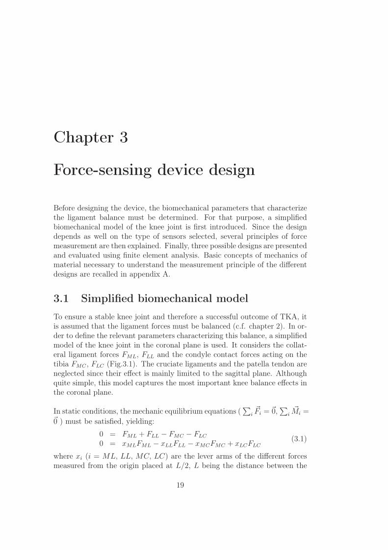
Before designing the device, the biomechanical parameters that characterizethe ligament balance must be determined. For that purpose, a simplifiedbiomechanical model of the knee joint is first introduced. Since the designdepends as well on the type of sensors selected, several principles of forcemeasurement are then explained. Finally, three possible designs are presentedand evaluated using finite element analysis. Basic concepts of mechanics ofmaterial necessary to understand the measurement principle of the differentdesigns are recalled in appendix A.
3.1 Simplified biomechanical modelTo ensure a stable knee joint and therefore a successful outcome of TKA, itis assumed that the ligament forces must be balanced (c.f. chapter 2). In or-der to define the relevant parameters characterizing this balance, a simplifiedmodel of the knee joint in the coronal plane is used. It considers the collat-eral ligament forces FML, FLL and the condyle contact forces acting on thetibia FMC , FLC (Fig.3.1). The cruciate ligaments and the patella tendon areneglected since their effect is mainly limited to the sagittal plane. Althoughquite simple, this model captures the most important knee balance effects inthe coronal plane.
In static conditions, the mechanic equilibrium equations (∑
i�Fi = �0,
∑i�Mi =
�0 ) must be satisfied, yielding:
0 = FML + FLL − FMC − FLC
0 = xMLFML − xLLFLL − xMCFMC + xLCFLC(3.1)
where xi (i = ML, LL, MC, LC) are the lever arms of the different forcesmeasured from the origin placed at L/2, L being the distance between the
19

20 CHAPTER 3. FORCE-SENSING DEVICE DESIGN
FMLFML
FMCFMC FLCFLC
FLLFLL
x
y
z
Figure 3.1: Two-dimensional knee joint modelThe patella tendon and the cruciate ligaments being mainly effective in the sagittal
plane, only the collateral ligament forces (FML, FLL) and the contact forces (FMC , FLC)are taken into account.
collateral ligaments. The lever arms of the collateral ligaments being L/2,equation (3.1) becomes:
Mnet = xMCFMC − xLCFLC =L
2(FML − FLL) (3.2)
where Mnet is the net varus-valgus moment of the contact forces actingon the knee joint. When the tension in the collateral ligaments is equal(FML = FLL), the right side of the equation is zero. Therefore, Mnet maybe regarded as the parameter characterizing the ligament imbalance, andreducing it to zero is equivalent to balancing the ligaments. In conclusion,the device must be able to either measure this net varus-valgus moment ormeasure parameters that allow its computation.
3.2 Techniques to measure forcesAs a force can not be measured directly, its effect on a body, such as theresulting deformation or displacement, must be assessed. For example, thestrain experienced at the base of a bending beam is directly proportional to
3.2. TECHNIQUES TO MEASURE FORCES 21
the force applied at the beam extremity by the well-known flexure formula(c.f. equation (A.22)). Four types of force sensors have been investigated forour application: capacitive, magnetic, inductive sensors and strain gauges.
3.2.1 Capacitive sensors
A capacitor is schematically represented by two conductors separated by agap. Its capacitance is a function of the area S of the conductors and thegap d:
C = εS
d, (3.3)
where ε is the dielectric constant of the gap. According to equation (3.3) agap change, which is a relative displacement of the conductors, leads to avariation in the capacitance.
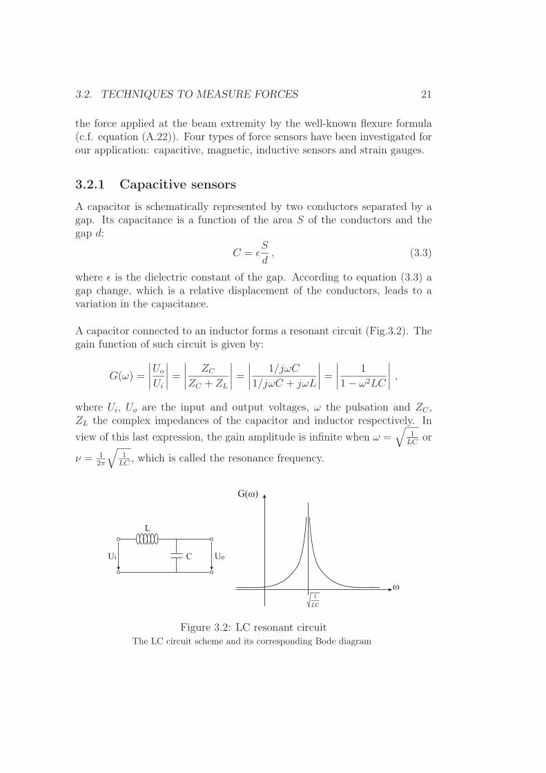
A capacitor connected to an inductor forms a resonant circuit (Fig.3.2). Thegain function of such circuit is given by:
G(ω) =
∣∣∣∣Uo
Ui
∣∣∣∣ =
∣∣∣∣ ZC
ZC + ZL
∣∣∣∣ =
∣∣∣∣ 1/jωC
1/jωC + jωL
∣∣∣∣ =
∣∣∣∣ 1
1 − ω2LC
∣∣∣∣ ,where Ui, Uo are the input and output voltages, ω the pulsation and ZC ,ZL the complex impedances of the capacitor and inductor respectively. Inview of this last expression, the gain amplitude is infinite when ω =
√1
LCor
ν = 12π
√1
LC, which is called the resonance frequency.
L
CUi Uo
1
LC
G( )�
�
Figure 3.2: LC resonant circuitThe LC circuit scheme and its corresponding Bode diagram

22 CHAPTER 3. FORCE-SENSING DEVICE DESIGN
Capacitive sensors can therefore be placed in such a manner that the ap-plication of a force makes d or S, and thereby the capacitance C, vary. Byintegrating the sensor in a resonant circuit, the applied force can be retrievedby measuring the change of the resonance frequency.
3.2.2 Magnetic, inductive sensors
Another possibility to measure forces is to use magnetic or inductive sen-sors. In both cases, the measurement system is composed of an emitter anda receiver. The emitter generates a magnetic field and is mounted on a partof the sensing device which is deformed by the applied load. The receiveris placed on a fixed reference part and measures the variation of the mag-netic field induced by the emitter displacement. Since the emitter positionis dependent on the applied load, a direct relationship exists between themagnetic field variation measured by the receiver and the applied load.
The measurement principle of the magnetic and inductive sensors is as fol-lows:
1. Magnetic sensors
• The emitter is a permanent magnet.
• The receiver is a magnetic field detector based on the Hall effect(Fig.3.3). When a electrical current traverses a metallic plate sub-merged in a magnetic field, the electrons going through the plateexperience a Lorentz force perpendicular to the current direction.A measurable voltage, whose amplitude varies proportionally tothat of the magnetic field, appears at its border.
B
Ie-
V=0
V=VH
Figure 3.3: Illustration of the Hall effectWhen an electrical current (I) traverses a metallic plate submerged in a magnetic field
(B), the electrons are deviated and a voltage (VH) is generated at the borders.

3.2. TECHNIQUES TO MEASURE FORCES 23
2. Inductive sensors
• The emitter is a coil powered by an alternative current, thus gen-erating an oscillating magnetic field.
• The receiver is a coil too, into which the emitted magnetic fieldinduces a current. The amplitude of the induced current varieswith the magnetic field amplitude.
3.2.3 Strain gauges
A strain gauge is a device whose electrical resistance varies in proportion tothe amount of strain in the device. The most widely used gauge is the bondedmetallic strain gauge. The metallic strain gauge consists of a fine wire or,more commonly, metallic foil arranged in a grid pattern. The grid patternmaximizes the amount of wire to strain in the direction parallel to the gaugebacking (Fig.3.4). The cross-sectional area of the grid is minimized to reducethe effect of shear strain and Poisson strain (c.f. appendix A). The grid isbonded to a thin backing, which is attached directly to the test specimen.Therefore, the strain experienced by the test specimen is transferred directlyto the strain gauge, which responds with a linear change in electrical resis-tance due to the lengthening or shortening of the metallic foil.
Figure 3.4: Metallic strain gaugeA strain gauge is basically a thin wire arranged in a grid pattern whose resistance
linearly varies with the strain.
Although this low-cost technology gives a large freedom to the designer, afew delicate points such as the bonding and the positioning have to be con-sidered. It is very important that the strain gauge is properly mounted ontothe test specimen so that the strain is accurately transferred from the testspecimen, through the adhesive and strain gauge backing, to the foil itself.Bad mounting not only affects the measurement sensitivity, but also causes

24 CHAPTER 3. FORCE-SENSING DEVICE DESIGN
self-heating problems. Inaccurate positioning, such as bad parallelism, gen-erates deviations by not measuring the desired force, but only its projectionon the gauge axis.
Piezoresistive sensors
To overcome the disadvantages of bonded metallic strain gauges, piezore-sistive ceramic elements can be used instead (c.f. chapter 4). In additionto a larger gauge factor, which is the ratio between the strain and resis-tance variation, and a larger resistance, which reduces the self-heating dueto the Joule effect, thick-film piezoresistive sensors can be directly depositedon the specimen by screen printing. With such technology, errors due tobad mounting are minimized. Furthermore, the size of piezoresistive sensorsare significantly reduced compared to that of standard strain gauges, thusallowing finer designs.
3.2.4 Choice of the measurement principle
Although each of the previously discussed sensor types could be used, thick-film piezoresistive sensors have been chosen for the following reasons:
• The measurement principle is relatively simple.
• The encumbrance is not significant.
• The intrinsic accuracy of the sensor is high.
• It is a low-cost technology.
• The signal conditioning can be ensured with just an amplifier and afilter.
• Standard heat moisture sterilization is possible.
• Biocompatibility can be easily ensured by a final surface coating.

3.3. DEFINITION, EVALUATION OF POSSIBLE DESIGNS 25
3.3 Definition, evaluation of possible designsBefore describing in details the three designs, the common aspects, such asthe perimeter, the different parts composing the device and the material se-lected are presented.
The three conceived designs were inspired from existing prosthetic compo-nents. The perimeter of the device was extracted from a CKS inlay (Biomet,Warsaw, IN, USA). It is 77mm wide and 51mm long, so it is suitable fortibias of medium size. In case of routine clinical use, the device would beavailable in different scales to cover all the possible knee sizes.
A flat reference surface on the tibial side is required to ensure reliable mea-surements. Moreover, compressive forces or varus-valgus moments have tobe assessed with different knee gaps to comply with the surgical procedure.For these reasons, the device is composed of three distinct parts:
1. A tibial base plate, which is fixed by pins on the tibia after a tibial cutand serves as a reference plate.
2. A sensitive plate, which measures the moments and which lies on thebase plate.
3. A set of spacers, which allows measurements at different knee gaps.
Finally, the material used for the sensitive plate has to be:
1. Biocompatible. Biocompatibility is the quality of not having toxic orinjurious effects on biological systems. There exist different degrees ofbiocompatibility, depending on the amount of time the material has tobe in contact with the human body, especially with bones and bod-ily fluids. Although the device operates for less than half an hour,implantable material should be used in order to preserve the patientsafety in case of accidental release of debris.
2. Compatible with thick-film technology. Up to now, the deposition pro-cess is controlled for stainless steel based applications. The high curingtemperature during deposition limits the choice of material and preventthe usage of metals with better properties for a force-sensing device,such as titanium.
3. Suitable mechanical properties. The selected material must have suit-able mechanical properties for a force-sensing device, i.e. a large elastic
26 CHAPTER 3. FORCE-SENSING DEVICE DESIGN
range and a high ultimate stress. Moreover, as the device is heatedduring the sensors curing, it must have these properties in annealedconditions.
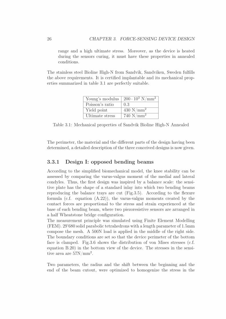
The stainless steel Bioline High-N from Sandvik, Sandviken, Sweden fulfillsthe above requirements. It is certified implantable and its mechanical prop-erties summarized in table 3.1 are perfectly suitable.
Young’s modulus 200 · 103 N/mm2
Poisson’s ratio 0.3Yield point 430 N/mm2
Ultimate stress 740 N/mm2
Table 3.1: Mechanical properties of Sandvik Bioline High-N Annealed
The perimeter, the material and the different parts of the design having beendetermined, a detailed description of the three conceived designs is now given.
3.3.1 Design I: opposed bending beams
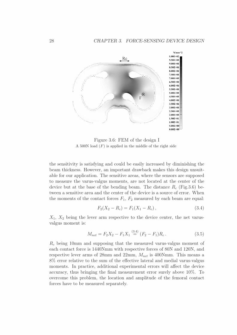
According to the simplified biomechanical model, the knee stability can beassessed by comparing the varus-valgus moment of the medial and lateralcondyles. Thus, the first design was inspired by a balance scale: the sensi-tive plate has the shape of a standard inlay into which two bending beamsreproducing the balance trays are cut (Fig.3.5). According to the flexureformula (c.f. equation (A.22)), the varus-valgus moments created by thecontact forces are proportional to the stress and strain experienced at thebase of each bending beam, where two piezoresistive sensors are arranged ina half Wheatstone bridge configuration.The measurement principle was simulated using Finite Element Modelling(FEM). 29’680 solid parabolic tetrahedrons with a length parameter of 1.5mmcompose the mesh. A 500N load is applied in the middle of the right side.The boundary conditions are set so that the device perimeter of the bottomface is clamped. Fig.3.6 shows the distribution of von Mises stresses (c.f.equation B.20) in the bottom view of the device. The stresses in the sensi-tive area are 57N/mm2.
Two parameters, the radius and the shift between the beginning and theend of the beam cutout, were optimized to homogenize the stress in the

3.3. DEFINITION, EVALUATION OF POSSIBLE DESIGNS 27
Figure 3.5: 3D model of design ITwo bending beams allow the measurement of the varus-valgus moments of the medial
and lateral femoral condyles.
sensitive areas of the device in order to minimize the stress variation alongthe piezoresistive sensors (Fig.3.7):
1. A small cutout radius generates stress concentrations and a large re-duces the beam width, both being able to provide stresses exceeding thematerial limit. A good indicator of an homogeneous stress distributionis the ratio between the maximal and average stresses. As this ratiothis ratio nears 1, the stress distribution becomes more homogeneous.This ratio was therefore calculated by FEM for different cut radii andshowed that the optimal radius is 6mm.
2. As the contact point of each condyle is not expected to lie in the centerof the beam but rather in the center of the left or right part of thedevice, the beam rotation axis is not perpendicular to the beam itself.To facilitate the placement of the sensors, which should be on the beamrotation axis where the stress is theoretically maximal, the perpendic-ularity has to be restored. This can be carried out by imposing a shiftbetween the beginning and the end of the beam cutout. To determinethe optimal shift, the stress variations along the axis perpendicular tothe beam and going by the point of maximal stress was computed byFEM for different shift amplitudes. The variations are minimal with ashift of 5.6mm.
At first sight, this design seems adequate. The stresses are smoothly dis-tributed in the sensitive area and the ratio of 1.7 between the maximal andaverage stresses gives a reasonably homogeneous sensitive area. Moreover,
28 CHAPTER 3. FORCE-SENSING DEVICE DESIGN
Figure 3.6: FEM of the design IA 500N load (F ) is applied in the middle of the right side
the sensitivity is satisfying and could be easily increased by diminishing thebeam thickness. However, an important drawback makes this design unsuit-able for our application. The sensitive areas, where the sensors are supposedto measure the varus-valgus moments, are not located at the center of thedevice but at the base of the bending beam. The distance Rc (Fig.3.6) be-tween a sensitive area and the center of the device is a source of error. Whenthe moments of the contact forces F1, F2 measured by each beam are equal:
F2(X2 −Rc) = F1(X1 −Rc) , (3.4)
X1, X2 being the lever arm respective to the device center, the net varus-valgus moment is:
Mnet = F2X2 − F1X1(3.4)= (F2 − F1)Rc . (3.5)
Rc being 10mm and supposing that the measured varus-valgus moment ofeach contact force is 1440Nmm with respective forces of 80N and 120N, andrespective lever arms of 28mm and 22mm, Mnet is 400Nmm. This means a8% error relative to the sum of the effective lateral and medial varus-valgusmoments. In practice, additional experimental errors will affect the deviceaccuracy, thus bringing the final measurement error surely above 10%. Toovercome this problem, the location and amplitude of the femoral contactforces have to be measured separately.

3.3. DEFINITION, EVALUATION OF POSSIBLE DESIGNS 29
Figure 3.7: Design optimizationThe radius and the shift between the beginning and end of the cutouts were optimized to
have maximal homogeneous stress areas
3.3.2 Design II: open load cell
To measure the amplitude and location of the femoral contact forces, threemeasurement points per condyle are necessary. The simplest way to real-ize that is to have a defined medial and lateral contact area attached to aframe by three deformable bridges (Fig.3.8). When the device is loaded, thesum of the stresses experienced by the three bridges is proportional to theamplitude of the applied force whereas the ratio determines its location. Toperform correctly, however, such a device needs a large and strong frame,rigid enough to absorb and homogeneously distribute the load. The roombeing restricted in our application, this condition can not be ensured and themeasurements could depend on the location of the contact points betweenthe frame and the tibial base plate. For a good accuracy and reliability of themeasurements, the contact points between the plates must be mechanicallywell defined. Therefore, two sensitive plates and two sets of three balls areused to avoid statically indeterminate conditions.
The thickness of the sensitive plates is 3mm. The contact areas have an in-ternal diameter of 19mm. The bridges are 4mm wide to leave enough spacefor the electrical connections, as well as 5mm long and 1mm thick to besensitive enough to the deformations. The large contours at the bridge ex-tremities avoid stress concentrations. Two piezoresistive sensors are placed ateach side of each bridge, with two working in compression and two in tension.A full Wheatstone bridge can thereby be used, increasing the measurementsensitivity and avoiding temperature drift. To prevent the femoral condylesfrom being damaged by the cuts, a plastic hat could be placed on the top ofthe sensitive plates.
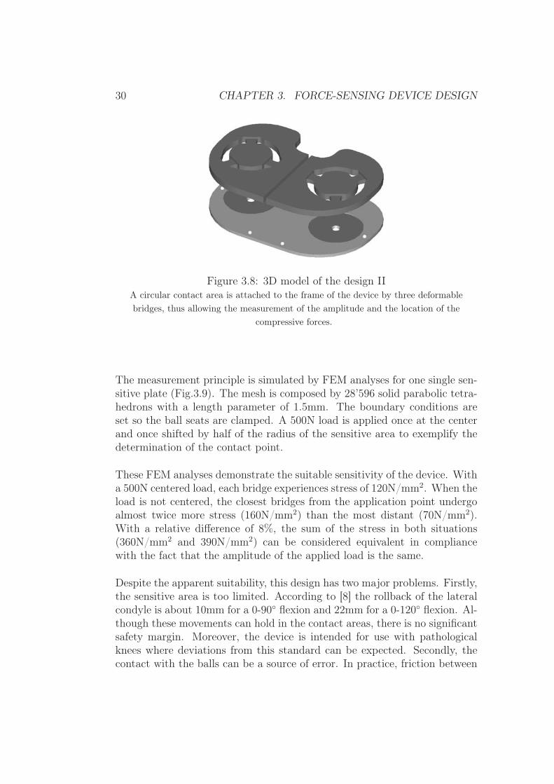
30 CHAPTER 3. FORCE-SENSING DEVICE DESIGN
Figure 3.8: 3D model of the design IIA circular contact area is attached to the frame of the device by three deformablebridges, thus allowing the measurement of the amplitude and the location of the
compressive forces.
The measurement principle is simulated by FEM analyses for one single sen-sitive plate (Fig.3.9). The mesh is composed by 28’596 solid parabolic tetra-hedrons with a length parameter of 1.5mm. The boundary conditions areset so the ball seats are clamped. A 500N load is applied once at the centerand once shifted by half of the radius of the sensitive area to exemplify thedetermination of the contact point.
These FEM analyses demonstrate the suitable sensitivity of the device. Witha 500N centered load, each bridge experiences stress of 120N/mm2. When theload is not centered, the closest bridges from the application point undergoalmost twice more stress (160N/mm2) than the most distant (70N/mm2).With a relative difference of 8%, the sum of the stress in both situations(360N/mm2 and 390N/mm2) can be considered equivalent in compliancewith the fact that the amplitude of the applied load is the same.
Despite the apparent suitability, this design has two major problems. Firstly,the sensitive area is too limited. According to [8] the rollback of the lateralcondyle is about 10mm for a 0-90◦ flexion and 22mm for a 0-120◦ flexion. Al-though these movements can hold in the contact areas, there is no significantsafety margin. Moreover, the device is intended for use with pathologicalknees where deviations from this standard can be expected. Secondly, thecontact with the balls can be a source of error. In practice, friction between

3.3. DEFINITION, EVALUATION OF POSSIBLE DESIGNS 31
Figure 3.9: FEM of the design IIA 500N load applied once at the center, once shifted to the right, shows the sensitivity as
well as the functioning
the balls and the base plate generates moments in the bridges which havenot been taken into account so far. The friction force is proportional to thereaction force (F ) which creates the moment in the bridge. Therefore, theratio between the moment that has to be measured and the moment due tofriction is given by:
µFd1
Fd2
=µd1
d2
. (3.6)
The lever arm of the friction moment (d1) is equivalent to the device thick-ness, i.e. 3mm. The distance between a bridge and the closest contact pointvaries from 10mm to 20mm (d2). A typical metal-to-metal friction coefficient(µ) being 0.2, the friction moment in a bridge corresponds to 3% to 6% ofthe effective moment. The device having six bridges, the total measurementerror due to friction is definitely not acceptable. To further optimize the de-sign, the contact area must be increased and the disturbances due to frictionmoment minimized.
3.3.3 Design III: integrated bridges
To maximize the contact area, the three bridges needed to measure the lo-cation and the amplitude of the femoral contact forces must be shifted to

32 CHAPTER 3. FORCE-SENSING DEVICE DESIGN
the device border (Fig.3.10). The bridges are 4mm wide and 4mm long tohave enough room for the sensors and their connections and 1mm thick toensure a good sensitivity. The bridge cutouts have been optimized by FEMin order to suppress stress concentrations while keeping a sufficiently largecontact area. The fillet under the bridges has a 1mm radius, which followsthe empirical rule stating that a fillet as large as the bridge thickness allowsavoiding stress concentrations. A ball is inserted in each pillar extremity toensure mechanically well defined contact points between the tibial base plateand the sensitive plates. Moreover, since these balls allow rotations, torsionis avoided and the bridges undergo pure bending.
Figure 3.10: 3D model of design IIIThe three bridges are placed at the device border to maximize the sensitive area and a
symmetrical bridge is used to minimize error due to friction moments. When a load F isapplied on the device, three reaction forces Ri (i = 1, 2, 3), whose amplitude depend onthe amplitude and location of the original load, are generated. The deformation of each
bridge due to a single reaction force is then measured.
The measurement principle is as follows: when a load �F is applied in thesensitive area, three reaction forces �R1, �R2 and �R3 are generated at thebridge pillars. The amplitude of those reaction forces is directly relatedto the location and amplitude of the applied load through the equilibriumequations: ∑
i
�Ri + �F = 0
∑i
�Xi ∧ �Ri + �X ∧ �F = 0 , (3.7)
where �Xi, i = 1, 2, 3 are the respective lever arms. As all the forces are

3.3. DEFINITION, EVALUATION OF POSSIBLE DESIGNS 33
perpendicular to the plate surface, the previous vectorial equations comedown to three independent scalar equations:
x1R1 + x2R2 + x3R3 − xF = 0
y1R1 + y2R2 + y3R3 − yF = 0 (3.8)R1 +R2 +R3 − F = 0 ,
which can be solved for F , x, y.
F = R1 +R2 +R3
x =x1R1 + x2R2 + x3R3
R1 +R2 +R3
(3.9)
y =y1R1 + y2R2 + y3R3
R1 +R2 +R3
Due to the difference of rigidity between the bridges and the rest of the sen-sitive plates, each bridge is deformed by the reaction force experienced byits own pillar. Everything occurs as if each bridge was laterally clamped anda single force applied at its center. In such situation, one compression andone tension domain appears at each side of the bridge pillar (Fig.3.11). Theamplitude of the reaction forces can be measured with four piezoresistivesensors placed at these specific locations (c.f. appendix A) and arranged in afull Wheatstone bridge. The location and amplitude of the applied load canthen be calculated thanks to equation (3.9).
Figure 3.11: Deformation of a single bridgeThe sides of the bridge are clamped and a load is applied at the center. Two compression
and tension areas appear at each side of the pillar.

34 CHAPTER 3. FORCE-SENSING DEVICE DESIGN
With this design, the contact area is defined by a triangle, whose edges arelocated at the pillar centers. This triangle has a base of 22mm and a heightof 36mm, which is much larger than with the open load cell design. Anotheradvantage of such a bridge configuration is the self-compensation of error dueto friction moments. As the effect of friction has the same amplitude but anopposite sign at each side of a single bridge, it is electronically cancelled outby the Wheatstone bridge.
Fig.3.12 is a typical simulation by FEM of the device performance. 28’735solid parabolic tetrahedrons with a length parameter of 1mm compose themesh. The boundary conditions are set so the pillar extremities allow rota-tions but not translations. A 500N load is applied once centered and onceposteriorly shifted to illustrate the measurement principle. The maximalcompressive von Mises stress is 150N/mm2 and the maximal tensile stressis 210N/mm2 when the load is centered. This asymmetry comes from theoverall bending of the sensitive plate, which is added on the bridges, thusdecreasing the compression and increasing the tension stresses. However, thisasymmetry is not a problem in practice since contributions equal in amplitudeand sign cancel each other due to the full Wheatstone bridge configuration.
Figure 3.12: FEM of the design IIIA 500N load applied once at the center, once posteriorly shifted, shows the sensitivity as
well as the working principle

3.3. DEFINITION, EVALUATION OF POSSIBLE DESIGNS 35
Finally particular attention must be paid to the balls: a very small balldiameter creates huge contact pressure which can tear the tibial base plate.The hertzian theory is therefore used to verify that the selected material andgeometry support the loads involved in this application. From appendix B,it is known that the maximal pressure of a sphere in a spherical seat is givenby
Pmax =1
π3
√6
π2
F
(K1 +K2)2
(R1 −R2)2
R21R
22
, (3.10)
Ki =1 − ν2
i
πEi
i = 1, 2 .
E is the Young’s modulus, ν the Poisson’s ratio, i indexes the two bodies, Fthe load, R1 and R2 the radius of the ball and its seat. From this maximalcontact pressure, the corresponding effective stress or von Mises stress, whichcan be compared to the material specifications given by the manufacturer,can be calculated using the relationship (c.f. appendix B):
σmaxeff = 0.6Pmax . (3.11)
Since the Sandvik High-N stainless steel would not support the contact pres-sure, titanium has been chosen for its biocompatibility and its relatively lowYoung’s modulus (c.f. Table 3.2), which decreases the maximal pressure ac-cording to equation (3.10).
Young’s modulus 114 · 103 N/mm2
Poisson’s ratio 0.34Yield point 870 N/mm2
Ultimate stress 950 N/mm2
Table 3.2: Mechanical properties of Titanium Grade 5 ELI
The diameter of the balls is 3mm and corresponds to the largest diameterallowing press-fit in the pillars. The seat in the base plate is 3.5mm andfollows from a trade off between the pressure amplitude and the manufactur-ing precision. On one hand, the seat diameter should be as close to the balldiameter as possible to maximize the contact area and therefore minimizethe contact pressure. On the other hand, it should be large to minimizethe errors induced by the manufacturing accuracy: a shift between the ballsand the seat location would lead to reaction forces not parallel to the pillars,
36 CHAPTER 3. FORCE-SENSING DEVICE DESIGN
thus inducing measurement errors. As the selected steel balls are normallyused in ball bearings and can support a pressure as large as 4’200N/mm2 be-fore reaching their yield point, only the titanium plate has to be inspected.With the numerical values presented above, the 870N/mm2 yield point oftitanium is reached with a load of 270N: more than half of the maximal loadcan be supported by a single pillar without yielding, which is sufficiently safe.
In conclusion, this design fulfills the requirements and shows important de-cisive advantages:
• Accurate measurement of force amplitude and location
• Mechanical decoupling between the medial and lateral sides
• Maximal contact area
• Minimal parasite effects (temperature drift, friction moments)
• Small size and thickness
• Possibility to keep the patella at its anatomical place during the mea-surement
• Sterilizable
This last design has therefore been considered as optimal and a series ofprototypes were built.
Extension of the sensitive area
Although the sensitive area has been maximized, the contact points of thefemoral condyles can be located close to the lateral device borders due to de-formities or unusual anatomy. Such cases would be out of the sensitive areaand therefore not measurable. In addition to this, the sensitive plate shouldbe fastened to the base plate in order to avoid lift-off during manipulationsor in absence of compressive forces.
To address these two issues, a fixation mechanism was developed (Fig.3.13).It has a T-shape whose pillar is screwed to the base plate and whose armscover the posterior medial bridge of each sensitive plate. A screw with aspherical head placed at each arm’s extremity allows the bridges to be fixed.The spherical screw head enables rotations, thus avoiding torsion in thebridge. With this system, the posterior medial bridge can measure verticalreaction forces in both directions, which allows the measurement of contact

3.3. DEFINITION, EVALUATION OF POSSIBLE DESIGNS 37
Figure 3.13: Fixation mechanismA T-shape mechanical part allows the posterior medial bridge of each sensitive plate to
be fastened to the tibial base plate.
forces located close to the lateral edge of the device. The same calibrationmodel can be used since the only change is the sign of the output voltagereflecting the direction of the reaction force. In addition to extending the sen-sitive area, this fixation mechanism enables the sensitive plates to be rigidlyfastened to the tibial base plate. Thus, the different parts constituting thedevice can be introduced as one piece into the knee, which improves theergonomics of the device.
Spacers
As previously mentioned, a set of medial and lateral spacers are needed toadapt the device thickness to the patient-specific tibiofemoral gaps. Fromthe engineer’s point of view, the best solution would be to intercalate spac-ers between the tibial base plate and the sensitive plates. By doing so, thefemoral condyles are directly in contact with the sensitive plates, thus en-suring an optimal output signal. However, this solution would significantlydiminish the device ergonomics since the fixation mechanism would need tobe replaced each time a thicker spacer is used. To overcome this disadvan-tage, spacers should be placed on the top of the sensitive plates. Particularattention must therefore be paid to the shape of the spacers and the materialused to keep accurate measurements.
Thin adaptor spacers (2mm) are placed directly on the top of the sensitiveplates to ensure a correct transmission of applied loads to the sensitive area(Fig.3.14). Medial, lateral and posterior cutouts allow accommodating thewires and the fixation mechanism. The bottom surface follows the contour ofthe sensitive area to enable the deformation of the sensitive plates. If these

38 CHAPTER 3. FORCE-SENSING DEVICE DESIGN
adaptor spacers would lie on the bridges, applied loads would be withstoodby the reaction forces in the bridge pillars without producing any beam de-formation. Two rectangular extrusions designed to fit in the sensitive platecutouts avoid rotations and translations of the spacer. Finally, the top sur-face has an anterior elliptical extrusion which serves as an attachment pointfor the additional block spacers (Fig.3.14). These latter have thicknessesranging from 1mm to 10mm. A posterior cutout allows accommodating thefixation mechanism and a bottom anterior conical hole enables the blockspacers to be plugged into the adaptor spacers.
(a) Top view (b) Bottom view
Figure 3.14: SpacersThin adaptor spacers, onto which block spacers of different thicknesses can then be
plugged, are used to ensure a correct transmission of applied loads to the sensitive area.
The reliability of the load transmission through the spacers depend not onlyon the geometry but also on the material used. To ensure an optimal se-lection, the contact pressure distribution at the bottom surface of a spacerwas analyzed by FEM for different materials. The model consisted of a 5mmthick spacer placed on a single sensitive plate. The contact condition wascarried out by a penalty method. The meshes of the spacer and the sensitiveplate were composed by 5931 and 4927 tetrahedron elements respectively,with a length parameter of 1mm. A 100N vertical force was applied to thetop of the spacer, at the center of the sensitive area. The contact pressuredistribution was then calculated for four different materials: stainless steel,aluminium, and polyethylene with a 10GPa or 1GPa Young modulus.

3.3. DEFINITION, EVALUATION OF POSSIBLE DESIGNS 39
(a) Stainless steel (b) Aluminium
(c) PE 10GPa (d) PE 1GPa
Figure 3.15: Spacers made of different materialsPressure distribution at the bottom surface of spacers made of stainless steel, aluminium,
or polyethylene with a Young modulus of 10GPa and 1GPa.
40 CHAPTER 3. FORCE-SENSING DEVICE DESIGN
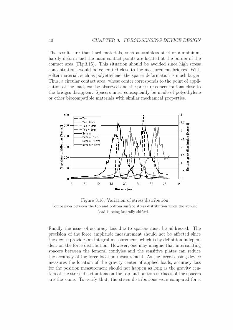
The results are that hard materials, such as stainless steel or aluminium,hardly deform and the main contact points are located at the border of thecontact area (Fig.3.15). This situation should be avoided since high stressconcentrations would be generated close to the measurement bridges. Withsofter material, such as polyethylene, the spacer deformation is much larger.Thus, a circular contact area, whose center corresponds to the point of appli-cation of the load, can be observed and the pressure concentrations close tothe bridges disappear. Spacers must consequently be made of polyethyleneor other biocompatible materials with similar mechanical properties.
Figure 3.16: Variation of stress distributionComparison between the top and bottom surface stress distribution when the applied
load is being laterally shifted.
Finally the issue of accuracy loss due to spacers must be addressed. Theprecision of the force amplitude measurement should not be affected sincethe device provides an integral measurement, which is by definition indepen-dent on the force distribution. However, one may imagine that intercalatingspacers between the femoral condyles and the sensitive plates can reducethe accuracy of the force location measurement. As the force-sensing devicemeasures the location of the gravity center of applied loads, accuracy lossfor the position measurement should not happen as long as the gravity cen-ters of the stress distributions on the top and bottom surfaces of the spacersare the same. To verify that, the stress distributions were compared for a

3.3. DEFINITION, EVALUATION OF POSSIBLE DESIGNS 41
100N load being shifted from the center to the border of the sensitive areaby steps of 5mm. For each step, the gravity center calculated by the FEMsoftware was identical for the top and bottom stress distributions. Fig.3.16also demonstrates this equivalence in a graphical way: the symmetry centerof the stress variation along a horizontal axis is the same for both distribu-tions. Therefore, no accuracy loss due to the intercalation of spacers shouldbe expected.
To conclude this chapter, the design of the complete device is shown in anexploded three-dimensional view (Fig.3.17).
Figure 3.17: Complete deviceExploded three-dimensional view of the complete device

42 CHAPTER 3. FORCE-SENSING DEVICE DESIGN

Chapter 4
Thick-film piezoresistive sensors
4.1 Piezoresistive effect
By definition, piezoresistive sensors are elements whose resistance varies inresponse to a mechanical stimulation. They can therefore be considered asstrain gauges, akin to metallic gauges, whose principle has been shortly ex-plained in section 3.2.3. A more elaborate technique is nevertheless used inorder to obtain a higher strain sensitivity as well as a good quality of thegauge bond to the substrate, usually a source of difficulties and errors withfoil gauges. A thick-film piezoresistive bridge, directly screen-printed andfired onto the steel substrate, was used. The sensing thick-film resistors aretypically composed of 85% of glass (PbO − SiO2 −B2O3 −Al2O3) and 15%of conductive oxide particles (RuO2 and Pb2Ru2O6). After sintering, the re-sistor material consists of an insulating glass matrix, in which the conductiveparticles form a percolating network. Charge transport between adjacentparticles is governed by tunnelling through a very thin (ca. 1nm) insulatinglayer. The interparticle resistance depends directly on the average distanced separating two charged particles. Therefore, when the sensor is strained,the average distance d is modified and the resistance varies accordingly. Thetunnelling effect and the local strain inhomogeneity [48, 49] account for therelatively high sensitivity ("gauge factor") of thick-film resistors, ca. 12 vs.ca. 2 for metal gauges.
A thick-film sensing bridge on steel requires at least three different materials:the insulating dielectric, the conductor and the piezoresistor. Usually, afourth protective glassy layer is applied over the circuit to improve chemicaland electrical stability.
43
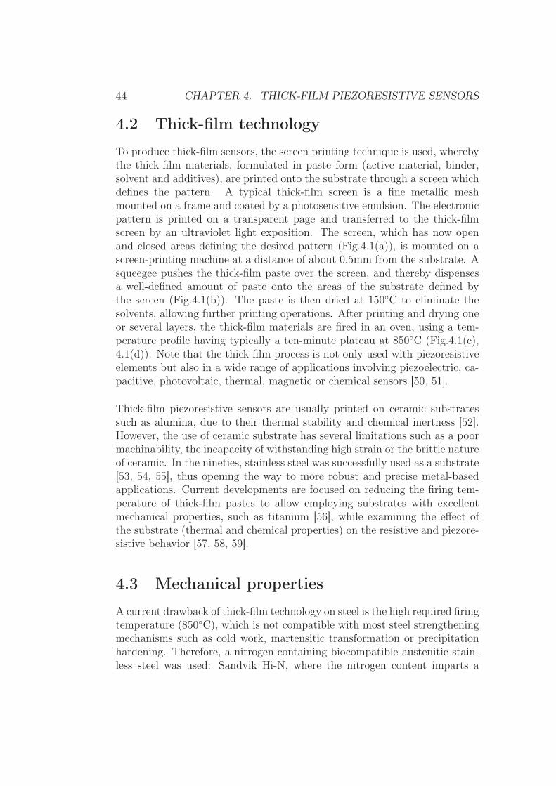
44 CHAPTER 4. THICK-FILM PIEZORESISTIVE SENSORS
4.2 Thick-film technology
To produce thick-film sensors, the screen printing technique is used, wherebythe thick-film materials, formulated in paste form (active material, binder,solvent and additives), are printed onto the substrate through a screen whichdefines the pattern. A typical thick-film screen is a fine metallic meshmounted on a frame and coated by a photosensitive emulsion. The electronicpattern is printed on a transparent page and transferred to the thick-filmscreen by an ultraviolet light exposition. The screen, which has now openand closed areas defining the desired pattern (Fig.4.1(a)), is mounted on ascreen-printing machine at a distance of about 0.5mm from the substrate. Asqueegee pushes the thick-film paste over the screen, and thereby dispensesa well-defined amount of paste onto the areas of the substrate defined bythe screen (Fig.4.1(b)). The paste is then dried at 150◦C to eliminate thesolvents, allowing further printing operations. After printing and drying oneor several layers, the thick-film materials are fired in an oven, using a tem-perature profile having typically a ten-minute plateau at 850◦C (Fig.4.1(c),4.1(d)). Note that the thick-film process is not only used with piezoresistiveelements but also in a wide range of applications involving piezoelectric, ca-pacitive, photovoltaic, thermal, magnetic or chemical sensors [50, 51].
Thick-film piezoresistive sensors are usually printed on ceramic substratessuch as alumina, due to their thermal stability and chemical inertness [52].However, the use of ceramic substrate has several limitations such as a poormachinability, the incapacity of withstanding high strain or the brittle natureof ceramic. In the nineties, stainless steel was successfully used as a substrate[53, 54, 55], thus opening the way to more robust and precise metal-basedapplications. Current developments are focused on reducing the firing tem-perature of thick-film pastes to allow employing substrates with excellentmechanical properties, such as titanium [56], while examining the effect ofthe substrate (thermal and chemical properties) on the resistive and piezore-sistive behavior [57, 58, 59].
4.3 Mechanical properties
A current drawback of thick-film technology on steel is the high required firingtemperature (850◦C), which is not compatible with most steel strengtheningmechanisms such as cold work, martensitic transformation or precipitationhardening. Therefore, a nitrogen-containing biocompatible austenitic stain-less steel was used: Sandvik Hi-N, where the nitrogen content imparts a

4.3. MECHANICAL PROPERTIES 45
(a) Thick-film screen (b) Paste deposition
(c) Oven (d) Sensor firing
Figure 4.1: Screen printing process
considerable solution strengthening effect, which is not affected by the thick-film firing process. To test the compatibility between the selected steel andthe thick-film piezoresistive sensors, deformable membranes have been man-ufactured (Fig.4.2(a)). Such pressure sensor is a reference device for materialcharacterization of the Laboratoire de Production Microtechnique, EPF Lau-sanne, Switzerland, the collaborative institute in charge of the production ofthe sensors.
Different pressure magnitudes were applied stepwise on the membrane gener-ating radial stresses (σr) up to 600MPa. The relative signal drift reported infigure 4.2(b) is lower than 0.1% for all the applied stresses. The softer stain-less steel DIN 1.4435, from which is branched off the biocompatible steel DIN1.4441 used for numerous surgical tools such as scalpels, pliers or chisels, hasstandard mechanical properties and is presented in the diagram for compar-ison. The obtained result demonstrates the proper functioning of the deviceand therefore the compatibility of the technique with the selected stainlesssteel.

46 CHAPTER 4. THICK-FILM PIEZORESISTIVE SENSORS
(a) Deformable membrane (b) Signal drift
Figure 4.2: Deformable membranes
4.4 Custom low-temperature dielectricDue to the high coefficient of thermal expansion (CTE) of the austeniticSandvik Hi-N steel (16.5 10−6/◦C), delamination due to thermal mismatchwith the thick-film layers may occur during the cooling phase following firing.Extensive problems were not observed on the simple membranes described inthe previous section, which only comprise a dielectric - conductor - piezore-sistor sequence, although local chipping at the edges of the printed dielectriclayer indicated extensive compressive stresses. Our force-sensing device, how-ever, is more complex than the membranes and requires additional dielectricand conductor layers to allow electric cross-overs. The resulting stress build-up proved fatal to the devices: extensive spallation in the thick-film circuitsoccurred in these cross-over zones.
Therefore, cross-overs were made with different materials: a commercial low-firing fritted silver conductor, together with a special low-stress dielectricdeveloped at EPFL. This low-firing dielectric consists of a dispersion of alu-mina powder in a low-melting lead borosilicate glass having a high CTE.The high CTE, together with the low softening temperature, results in verylittle additional stresses being developed in the cross-overs: no spallation wasobserved with the new materials. One must note that the present state ofthick-film technology does not allow the use of these materials for the maininsulating dielectric layer between the steel and the sensor circuit.

Chapter 5
Calibration and intrinsic accuracy
5.1 Calibration method
The calibration of a sensitive plate consists in establishing the numericalrelationship which converts the three measured voltages (M1, M2, M3) intothe corresponding location (x, y) and amplitude (F ) of the applied force.The calibration model results directly from equation (3.9), which describesthe measurement principle of the device, and is expressed by:
F = C11M1 + C12M2 + C13M3
x =C21x1C11M1 + C22x2C12M2 + C23x3C13M3
C11M1 + C12M2 + C13M3
(5.1)
y =C31y1C11M1 + C32y2C12M2 + C33y3C13M3
C11M1 + C12M2 + C13M3
.
The three first calibration coefficients (C11, C12, C13) correspond to the pro-portionality factor existing between the output voltage and the reaction forceamplitude of each bridge. The six last coefficients quantify the deviation ofthe experimental reality from the theoretical model in the x (C21, C22, C23)and y (C31, C32, C33) directions. In an ideal case, they should be 1.
To determine these nine coefficients, 16 points of measurements are used:four loads evenly distributed in the range 0-500N and four locations evenlydistributed on the sensitive area. As the determination of the six last cali-bration coefficients depends on the three first, the computation based on aleast square method is performed in two steps. Table 5.1 shows an exampleof a typical calibration matrix. As the most important deviation of the sixlast coefficients from the ideal value of 1 is 5% only, the calibration model is
47

48 CHAPTER 5. CALIBRATION AND INTRINSIC ACCURACY
considered correct and appropriate.
4.757 4.508 4.5801.009 1.007 1.0061.048 0.998 1.000
Table 5.1: Example of a calibration matrix
5.2 Intrinsic accuracyThe intrinsic accuracy of the device was evaluated by loading the sensitivearea with 18 weights ranging from 0N to 500N, applied at 20 different loca-tions evenly distributed (Fig.5.1). The positioning of the tip of the mecha-nism supporting the weights was controlled by a micrometer table (Fig.5.2).For each location, the different weights were applied incrementally.
Figure 5.1: Measurement points for the accuracy study
Figure 5.3 compares the measured force amplitudes and applied weights. Theclose-to-one slope (1.0009) and confidence parameter (1) of the linear regres-sion validates the measurement principle and demonstrates the absence ofsystematic errors. The absolute difference between the measured and ap-plied loads and locations are shown in the figures 5.4(a), 5.4(b) and 5.4(c).The maximum force amplitude and location error among the 360 measure-ments were 2.6N and 0.8mm, whereas the mean absolute errors were 0.7N

5.2. INTRINSIC ACCURACY 49
Figure 5.2: Set-up used for the accuracy study
and 0.3mm respectively. Note that the location measurement error decreaseswith increasing load. Since the location computation is based on a ratio be-tween the bridge voltages, the larger each voltage is, the better defined is theratio. The error of the applied weights (0.01N) and locations (0.001m) being
Figure 5.3: Force amplitude vs applied weight

50 CHAPTER 5. CALIBRATION AND INTRINSIC ACCURACY
negligible, the measured deviations characterize the intrinsic accuracy. Thedevice thus offers an 0.5% full scale accuracy for the force amplitude mea-surement and a submillimeter accuracy for the force location. Such accuracyis comparable to that of various commercial force-sensing devices based onstrain gauge technology and can be considered as excellent.
Since the passive compression forces of a human knee joint are expected tobe below 100N, a specific calibration can be performed to decrease the forceamplitude measurement error in this range. The coefficients obtained fromthe calibration of the same prototype with four loads ranging from 0N to100N instead of 0N to 500N are summarized in table 5.2 and are consistentwith their equivalent in table 5.1. Furthermore, the coefficients characteriz-ing the deviation from the calibration model are again very close to the idealvalue of 1, thus confirming the soundness of the calibration procedure.
4.796 4.568 4.4651.024 1.008 1.0041.037 1.001 1.000
Table 5.2: Calibration matrix for the range 0-100N
Figures 5.5(a), 5.5(b), 5.5(c) show the absolute difference between the mea-sured and applied loads and locations with the new calibration. This time,the maximum force amplitude and location error were 5.6N and 0.8mm,whereas the mean absolute errors were 1.0N and 0.3mm respectively. Asexpected, the location measurement errors were not affected by the newcalibration while the force amplitude error decreased in the range 0-100Nand increased in the range 100-500N. However, the mean force amplitudeerror remains comparable to that previously computed, thus demonstratingthat changing the calibration range amounts to redistributing the total er-ror. With a maximal measurement error of 1.5N in the range 0-100N, themeasurement accuracy of the force amplitude is below 2%, which is suitablefor the intended application.

5.2. INTRINSIC ACCURACY 51
(a) Absolute force error
(b) Absolute x location error
(c) Absolute y location error
Figure 5.4: Measurement errors with a calibration in the range 0-500N

52 CHAPTER 5. CALIBRATION AND INTRINSIC ACCURACY
(a) Absolute force error
(b) Absolute x location error
(c) Absolute y location error
Figure 5.5: Measurement errors with a calibration in the range 0-100N

5.3. ACCURACY IN THE EXTENDED SENSITIVE AREA 53
5.3 Accuracy in the extended sensitive areaTo verify the proper device functioning in the extended sensitive area createdby the fixation mechanism (c.f. section 3.3.3), the intrinsic accuracy was alsoevaluated close to the lateral edge. The same experimental set-up as in theprevious section was used. The device was loaded with 9 weights rangingfrom 0N to 100N applied at 15 different locations evenly distributed in theextended sensitive area. Figures 5.6(a), 5.6(b), 5.6(c) show the absolutedifference between measured and applied loads and locations. The maximalforce amplitude and location errors were 1.8N and 1.2mm, whereas the meanabsolute errors were 0.5N and 0.3mm respectively. With three values greaterthan or equal to 1mm, the accuracy of the location measurement is slightlydiminished. However, these errors were observed only with small weights,i.e. at low output voltage, and did not affect the average measurement error.It can thus be concluded that the accuracy close to the edge of the device isequivalent to that in the center.
5.4 Accuracy with spacersIn section 3.3.3, where the design of the spacers is presented, it has beenconcluded that the measurement accuracy is theoretically not affected bythe use of spacers placed on the top of the device. To verify that conclu-sion in practise, the device was loaded with four weights ranging from 0Nto 100N, applied at five different locations, without spacer and with spacersof 5mm and 10mm thickness. The maximal error, i.e. the maximal abso-lute difference between the measured and applied loads, was determined foreach measurement condition. Fig.5.7 shows that the use of spacers slightlyincreased the measurement error, which can be due to imperfect manufac-turing or border effects creating an asymmetric load distribution around thepoint of application. However, with maximal errors of 1.4N and 1.1mm, theaccuracy is still very satisfying and the ergonomic benefit of these top spacersare more important than the measured loss of accuracy.
5.5 Calibration and autoclave sterilizationFinally, the influence of sterilization on the calibration had to be evaluated.The device was loaded again with four weights ranging from 0N to 100Napplied at five different locations before and after steam sterilization (121◦,100% humidity, 20min.). No difference in measurement errors was found(Fig.5.8), thus demonstrating the autoclavability of the device.
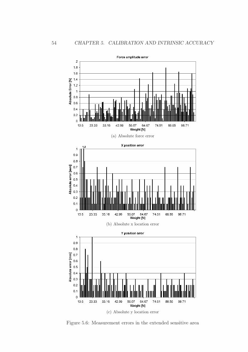
54 CHAPTER 5. CALIBRATION AND INTRINSIC ACCURACY
(a) Absolute force error
(b) Absolute x location error
(c) Absolute y location error
Figure 5.6: Measurement errors in the extended sensitive area

5.5. CALIBRATION AND AUTOCLAVE STERILIZATION 55
Figure 5.7: Accuracy loss due to spacers
Figure 5.8: Influence of sterilization on the calibration
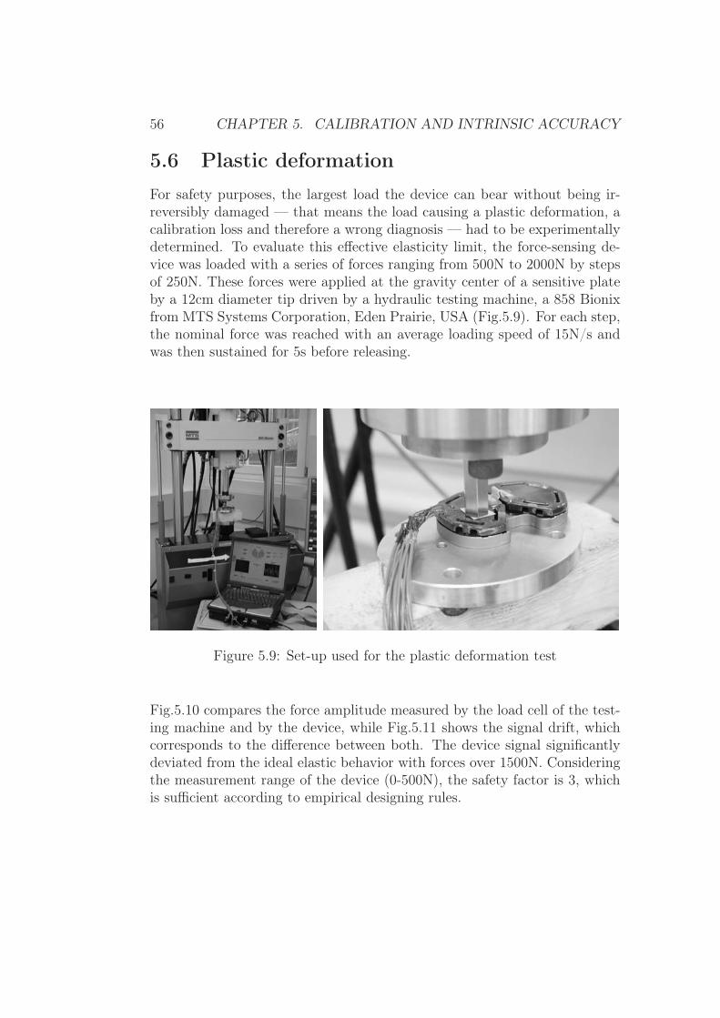
56 CHAPTER 5. CALIBRATION AND INTRINSIC ACCURACY
5.6 Plastic deformationFor safety purposes, the largest load the device can bear without being ir-reversibly damaged — that means the load causing a plastic deformation, acalibration loss and therefore a wrong diagnosis — had to be experimentallydetermined. To evaluate this effective elasticity limit, the force-sensing de-vice was loaded with a series of forces ranging from 500N to 2000N by stepsof 250N. These forces were applied at the gravity center of a sensitive plateby a 12cm diameter tip driven by a hydraulic testing machine, a 858 Bionixfrom MTS Systems Corporation, Eden Prairie, USA (Fig.5.9). For each step,the nominal force was reached with an average loading speed of 15N/s andwas then sustained for 5s before releasing.
Figure 5.9: Set-up used for the plastic deformation test
Fig.5.10 compares the force amplitude measured by the load cell of the test-ing machine and by the device, while Fig.5.11 shows the signal drift, whichcorresponds to the difference between both. The device signal significantlydeviated from the ideal elastic behavior with forces over 1500N. Consideringthe measurement range of the device (0-500N), the safety factor is 3, whichis sufficient according to empirical designing rules.

5.6. PLASTIC DEFORMATION 57
Figure 5.10: Comparison of MTS forces and device measurements
Figure 5.11: Signal drift during plastic deformation

58 CHAPTER 5. CALIBRATION AND INTRINSIC ACCURACY
In summary, the theoretical measurement principle was validated by the cal-ibration procedure and the obtained coefficients. Furthermore, the 0.5% fullscale accuracy and the safety factor of 3 meet the current industrial stan-dards and makes the device reliable. The accuracy in the extended sensitivearea and with the use of spacers is slightly reduced in practise, but still verysatisfying for the application. Finally, autoclave sterilization does not in-fluence the calibration. The device design has therefore been validated andthe evaluation of its ability to help the surgeon in ligament balancing is nowassessed with in-vitro studies.

Chapter 6
In-vitro study
Three different types of experiments were performed in order to validatethe device design and to evaluate the biomechanical influence of differentsurgical actions, such as a patellar eversion or a ligament release, on theligament balance.
6.1 Control experiment with a plastic modelTo assess the suitability of the device for the purpose of ligament balancing,the prototype was introduced in a plastic knee joint equipped with adjustablesprings. These latter simulated the collateral ligaments and the adjusting-screws of the side mechanisms allowed varying the spring tension (Fig.6.1).To validate that the varus-valgus moment measurements provided by ourdevice agree with defined imbalances, different spring tensions representingten levels of medial and lateral imbalance were applied. According to lawsof mechanics, it exists a linear relationship between these spring tensionsand the net varus-valgus moments of the tibiofemoral contact forces and thecorresponding proportionality factor is the lever arm of the spring forces.
The expected linear relationship between the measured net varus-valgus mo-ment of the contact forces and the spring tensions was experimentally verified(Fig.6.2). Furthermore, the measured proportionality factor (46mm) corre-sponded to the real lever arm (52mm) with a relative error of 13%. Thisdeviation is due to the cumulative effect of the intrinsic accuracy of the de-vice, the adjustment uncertainty of the spring tension and the play in themechanical fixation of the springs. The agreement between the theoreticalexpectations and the effective measurements demonstrates the device suit-ability for imbalance characterization in a well-controllable environment.
59
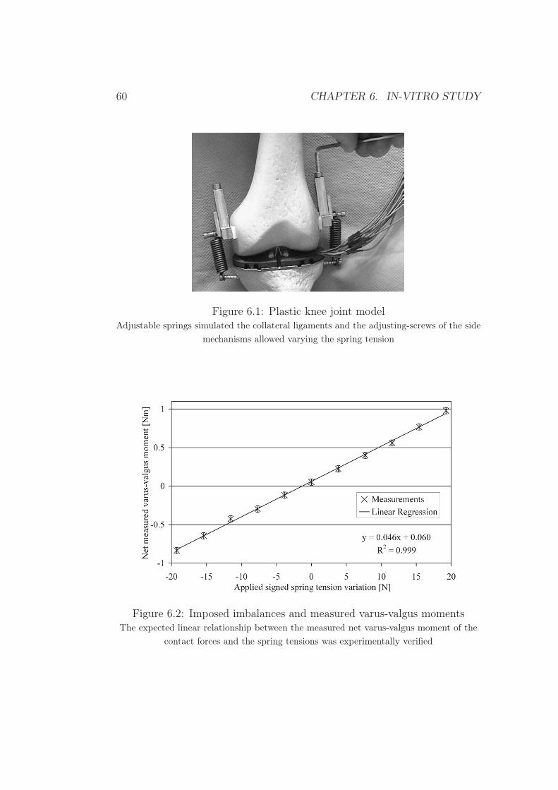
60 CHAPTER 6. IN-VITRO STUDY
Figure 6.1: Plastic knee joint modelAdjustable springs simulated the collateral ligaments and the adjusting-screws of the side
mechanisms allowed varying the spring tension
Figure 6.2: Imposed imbalances and measured varus-valgus momentsThe expected linear relationship between the measured net varus-valgus moment of the
contact forces and the spring tensions was experimentally verified

6.2. IN-VITRO TRIALS 61
6.2 In-vitro trialsIn order to verify the suitability of the range of measurement of the deviceand the consistency between the measurements and the surgeon’s perception,the prototype was tested in two cadaver specimens.
In the first experiment, the device was installed in the knee gap after a tib-ial cut of about 6mm. The medial and lateral femoral contact forces andthe net varus-valgus moment were measured during a ligament release pro-cedure. When no external forces were applied, the measured contact forcesranged from 40N to 70N. When the surgeon manually applied varus-valgusloads comparable to those that would be applied during a standard TKA, themaximal contact force reached 350-400N. Thus, the measurement range ofthe device (0-500N) is appropriate. The surgeon then performed a medial lig-ament release guided by the device measurements until the net varus-valgusmoment was reduced from an initial imbalance of 1.25Nm to 0.15Nm. Theobtained ligament balance was qualitatively consistent with the surgeon’sperception of a “balanced knee”.
In the second in-vitro trial, the tibiofemoral forces and moments were mea-sured in a balanced and imbalanced condition. Furthermore, five 90◦ kneeflexions were performed with two different degrees of ligament balance, whichwere realized using a) a 3mm lateral and medial spacers and b) a 6mm lateralspacer and a 3mm medial spacer. According to the surgeon’s judgment thesecond condition was better balanced than the first. In the balanced kneecondition, a lateral and a medial force amplitude of 24N and 22N were mea-sured. The relative difference of the respective varus-valgus moments was6%. In the imbalanced condition, the lateral and medial force amplitudeswere 36N and 9N, and the relative difference of the respective varus-valgusmoments was 60%. These results indicate that device measurements reflectthe surgeon’s perception. The averaged forces and moments measured duringthe flexion experiments are shown in Fig.6.3. In agreement to the surgeon’sopinion, the second condition exhibits a relative varus-valgus moment signif-icantly closer to 0.
In conclusion, the range of measurement of the device is suitable and themeasurements provided are in agreement with the surgeon’s perception.

62 CHAPTER 6. IN-VITRO STUDY
(a) Imbalanced
(b) Better balanced
Figure 6.3: Contact forces and moments during knee flexionTibiofemoral contact forces and varus-valgus moment during 90◦ knee flexions with two
different degrees of ligament balance

6.3. IN-SITU EVALUATION 63
6.3 In-situ evaluationFollowing these promising preliminary experiments, a complete in-vitro studywas carried out. The three primary goals were:
1. To evaluate the in-situ functioning and potential clinical advantages ofthe novel force-sensing device.
2. To identify the biomechanical parameter that the surgeon intraopera-tively assesses during ligament balancing. Each measurement systemdescribed in section 2.4 and aimed at providing a quantitative mea-surement of the ligament imbalance measures a different biomechani-cal parameter: Winemaker [44] measures extension gaps, Morris et al.[41] compressive forces, Takahashi et al. [39] and Wallace et al. [36]pressure and finally Attfield et al. [35] angular deviations of a scale-like device. This indicates that there is no standard interpretation ofwhat the surgeon intuitively calls ligament balancing in biomechanicalterms.
3. To quantify the effect of collateral ligament release in terms of forces.Even though ligament release is a commonly used surgical action tocorrect imbalance, its biomechanical effect in terms of knee joint forcesis poorly documented.
6.3.1 Method
The force-sensing device was tested in six human cadaver knees from donorswith an average age of 82 years (63 to 90). The surgical preparation ofeach specimen consisted of the two first steps of TKA, i.e. accessing thejoint with a medial parapatellar approach followed by the resection of thetibial plateau. The force-sensing device was then introduced (Fig.6.4) andthe specimen mounted on a knee joint loading apparatus (Fig.6.5) previouslydescribed by Dürselen at al. [60]. This machine provides all the degrees offreedom needed for unconstrained knee motion and allows the monitoringof the relative angular position between the femur and tibia. Compressionloads and varus-valgus moments can be applied by using a system of weightsand pulleys. Additionally, quadriceps forces can be simulated by loading thepatellar tendon with weights.
To validate the in-situ measurement of forces, the knee joint was first loadedin full extension with axial compressive weights ranging from 1kg to 15kg.The sum of the medial and lateral contact forces measured by the device,
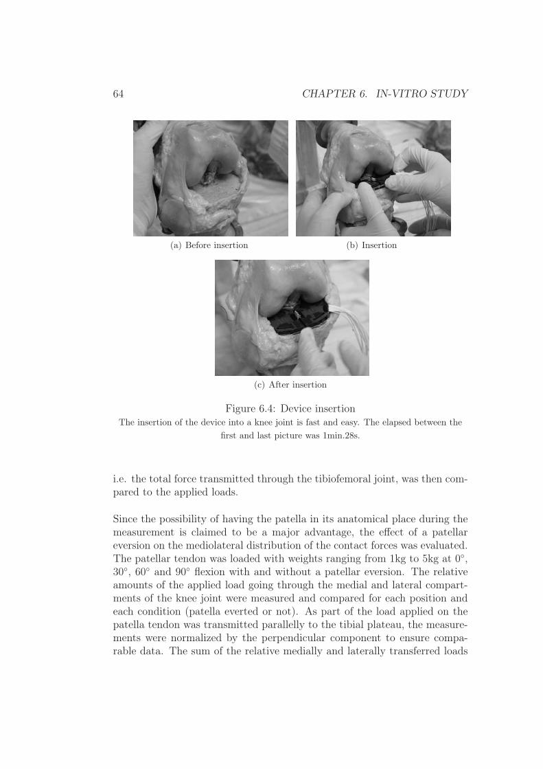
64 CHAPTER 6. IN-VITRO STUDY
(a) Before insertion (b) Insertion
(c) After insertion
Figure 6.4: Device insertionThe insertion of the device into a knee joint is fast and easy. The elapsed between the
first and last picture was 1min.28s.
i.e. the total force transmitted through the tibiofemoral joint, was then com-pared to the applied loads.
Since the possibility of having the patella in its anatomical place during themeasurement is claimed to be a major advantage, the effect of a patellareversion on the mediolateral distribution of the contact forces was evaluated.The patellar tendon was loaded with weights ranging from 1kg to 5kg at 0◦,30◦, 60◦ and 90◦ flexion with and without a patellar eversion. The relativeamounts of the applied load going through the medial and lateral compart-ments of the knee joint were measured and compared for each position andeach condition (patella everted or not). As part of the load applied on thepatella tendon was transmitted parallelly to the tibial plateau, the measure-ments were normalized by the perpendicular component to ensure compa-rable data. The sum of the relative medially and laterally transferred loads

6.3. IN-SITU EVALUATION 65
Figure 6.5: Knee joint loading apparatusThe arrows indicate the degrees of freedom of the machine, which allows unconstrainedknee motion. Compression loading (A), quadriceps force simulation (B) or varus-valgus
loading (C) can be carried out with a system of weights and pulleys.
then corresponds to 100%. The statistical significance was determined with asign test for paired samples (Matlab, MathWorks Inc, Natick, United States).
The second part of the study aimed at identifying the biomechanical param-eter that the surgeon assesses during ligament balancing. Intraoperatively,the surgeon manually compares the varus and valgus forces that must beapplied at the ankle to create a lateral or medial condyle lift-off. With a sim-plified two-dimensional model (Fig.6.6), it can be theoretically demonstratedthat this corresponds to a balancing of the medial and lateral condyle contactforces. The model considers the five major forces involved in the varus-valgusstability: the medial and lateral collateral ligament forces (FML, FLL), themedial and lateral contact forces (FMC , FLC) and an external varus force(FEX). The center of rotation, which in Fig.6.6 corresponds to the contactpoint of the medial condyle, is taken as the reference for the computation of
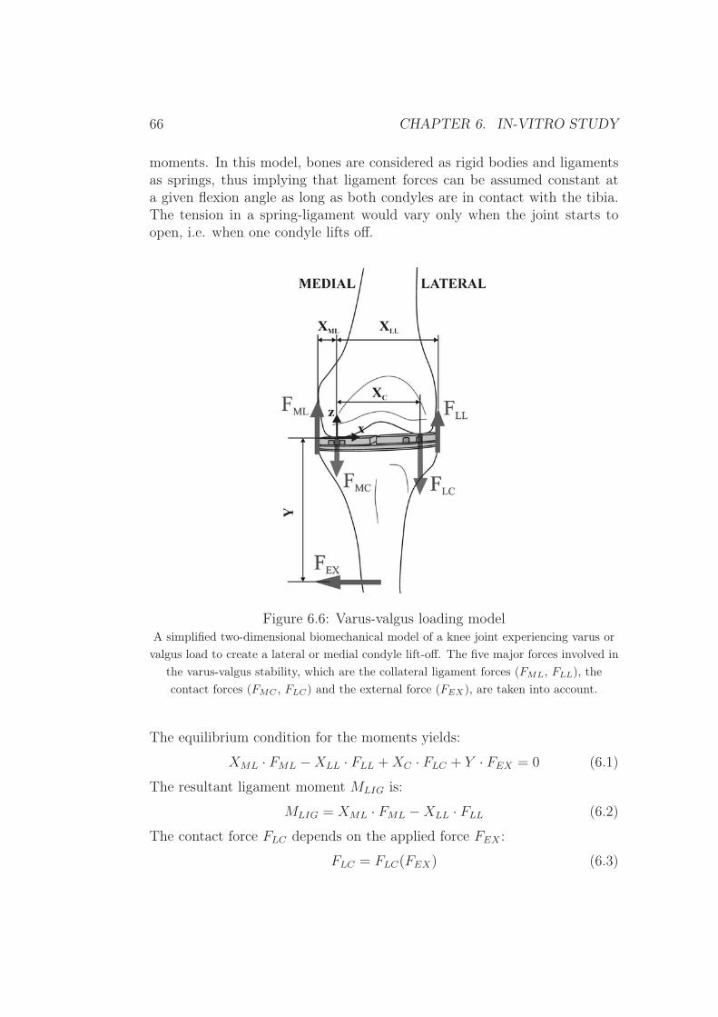
66 CHAPTER 6. IN-VITRO STUDY
moments. In this model, bones are considered as rigid bodies and ligamentsas springs, thus implying that ligament forces can be assumed constant ata given flexion angle as long as both condyles are in contact with the tibia.The tension in a spring-ligament would vary only when the joint starts toopen, i.e. when one condyle lifts off.
Figure 6.6: Varus-valgus loading modelA simplified two-dimensional biomechanical model of a knee joint experiencing varus orvalgus load to create a lateral or medial condyle lift-off. The five major forces involved in
the varus-valgus stability, which are the collateral ligament forces (FML, FLL), thecontact forces (FMC , FLC) and the external force (FEX), are taken into account.
The equilibrium condition for the moments yields:
XML · FML −XLL · FLL +XC · FLC + Y · FEX = 0 (6.1)
The resultant ligament moment MLIG is:
MLIG = XML · FML −XLL · FLL (6.2)
The contact force FLC depends on the applied force FEX :
FLC = FLC(FEX) (6.3)

6.3. IN-SITU EVALUATION 67
The combination of equations (6.1), (6.2), and (6.3) can then be written as:
MLIG +XC · FLC(FEX + Y · FEX = 0) (6.4)
When there is no external force applied (FEX = 0), equation (6.4) gives:
MLIG = −XC · FLC(0) (6.5)
When there is a varus load (FEX = Fvarus) that generates a lateral condylelift-off (FLC = 0), equation (6.4) gives:
MLIG = −Y · Fvarus (6.6)
The relationship between the varus load required for a condyle lift-off andthe initial lateral contact force can be deducted from equations (6.5) and(6.6):
Fvarus =XC
YFLC(0) (6.7)
The same approach can be adopted for the case of a valgus load and a medialcondyle lift-off:
Fvalgus =XC
YFMC(0) (6.8)
With equation (6.7) and (6.8) it can finally be concluded that the relativedifference of the forces required for a condyle lift-off is equal to the differenceof the contact forces:
Relative Imbalance =Fvarus − Fvalgus
Fvarus + Fvalgus
=FLC(0) − FMC(0)
FLC(0) + FMC(0)(6.9)
In order to experimentally validate this equivalence as well as to comparethis approach to the device measurements, the relative imbalance was as-sessed on the basis of three different parameters: 1) the weights required fora condyle lift-off, 2) the contact forces and 3) the varus-valgus moments. Theknee joint was therefore loaded with varus and valgus forces with weights in-creasing from 0kg to 1kg. If the condyle lift-off was not achieved before 1kg,larger weights were used. Since during the surgery the ligament imbalance isassessed in full extension and in 90◦ flexion, the experiment was performedin both positions.
In the third step, the biomechanical effect of medial collateral ligament re-leases was quantitatively evaluated. With interarticular spacers applyingstress to the ligaments, a minor followed by a major medial collateral liga-ment release was performed with the knee in full extension. The medial and

68 CHAPTER 6. IN-VITRO STUDY
lateral contact forces were recorded after each surgical action and comparedto the initial value. In order to quantify the effect of the ligament release onthe tibiofemoral alignment, the variation of the varus-valgus angle resultingfrom the releases was measured as well. Finally, the initial and ultimatecontact forces were measured at 0◦, 30◦, 60◦ and 90◦ flexion to evaluate theeffect of ligament releases throughout the knee flexion.
6.3.2 Results
All the curves obtained during the compression loading experiment werehighly linear (r2 = 1.00) and the measured slopes ranged between 0.96 and1.03, thus being very close to the ideal value of 1 (Fig.6.7). The averagedifference between the applied and measured compressive force was 1.8N.Thus, the in-situ force measurements are accurate and repeatable.
(a) Example of compression loading
knee 1 knee 2 knee 3 knee 4 knee 5 knee 6slope 1.03 0.98 1.03 0.96 1.00 0.98y-intercept -1.2 -1 -0.2 -1 0.3 -0.5
(b) Linear regression parameters
Figure 6.7: Compression loading experimenta) Comparison between the measured and applied forces during the compression loadingexperiment for one specimen. b) Parameters obtained from the linear regressions, which
demonstrate the accuracy and reliability of the in-situ force measurement.

6.3. IN-SITU EVALUATION 69
In the patellar load distribution experiment, the relative amounts of the ap-plied load going through the medial and lateral compartment of the knee jointwere measured. The mediolateral load distribution did not vary considerablywith knee flexion (standard deviations ranged from 3% to 8%), therefore thelaterally transferred loads were averaged over the different knee positions.The mediolateral distribution of the patellar load was significantly different(p=0.03) when the patella was in its anatomical place or not: one fourthof the patellar load was shifted from the medial to the lateral side with apatellar eversion (Fig.6.8). Additionally, it can be noted that the patella inits anatomical place already influenced the mediolateral distribution of thecontact forces since the average laterally transferred load was 62% withouta patellar eversion.
Figure 6.8: Effect of patellar eversionRelative laterally transferred loads during the patellar load distribution experiment,
showing that the patellar eversion significantly affected the mediolateral distribution ofthe contact forces. The grey and black horizontal lines correspond to the average loads
with the patella respectively in place or everted.
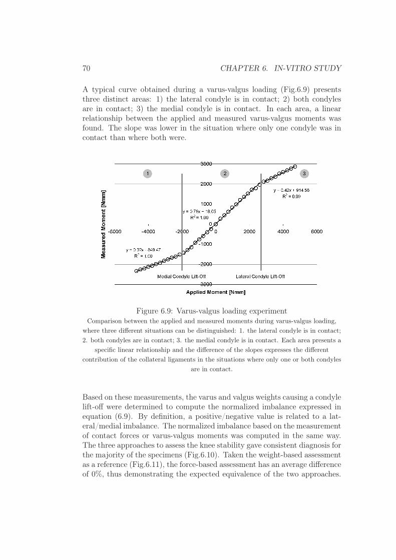
70 CHAPTER 6. IN-VITRO STUDY
A typical curve obtained during a varus-valgus loading (Fig.6.9) presentsthree distinct areas: 1) the lateral condyle is in contact; 2) both condylesare in contact; 3) the medial condyle is in contact. In each area, a linearrelationship between the applied and measured varus-valgus moments wasfound. The slope was lower in the situation where only one condyle was incontact than where both were.
Figure 6.9: Varus-valgus loading experimentComparison between the applied and measured moments during varus-valgus loading,
where three different situations can be distinguished: 1. the lateral condyle is in contact;2. both condyles are in contact; 3. the medial condyle is in contact. Each area presents a
specific linear relationship and the difference of the slopes expresses the differentcontribution of the collateral ligaments in the situations where only one or both condyles
are in contact.
Based on these measurements, the varus and valgus weights causing a condylelift-off were determined to compute the normalized imbalance expressed inequation (6.9). By definition, a positive/negative value is related to a lat-eral/medial imbalance. The normalized imbalance based on the measurementof contact forces or varus-valgus moments was computed in the same way.The three approaches to assess the knee stability gave consistent diagnosis forthe majority of the specimens (Fig.6.10). Taken the weight-based assessmentas a reference (Fig.6.11), the force-based assessment has an average differenceof 0%, thus demonstrating the expected equivalence of the two approaches.

6.3. IN-SITU EVALUATION 71
However, the moment-based assessment shows a tendency for lateral imbal-ance. Even though the average difference was small (6%), large differenceswere found in some cases, such as in the third knee. Similar results wereobtained for the measurements performed in 90◦ flexion but with an aver-age difference of imbalance of -4% and 7% respectively for the force-basedand moment-based assessments. The statistical significance, which was againdetermined with a sign test for paired samples, was achieved at 90◦ flexion(p=0.03), but not in full extension (p=0.38).
Figure 6.10: Comparison of imbalance assessmentAssessment of the relative ligament imbalance based on three different parameters: 1.the varus or valgus weights causing a condyle lift-off, 2. the contact forces and 3. the
varus-valgus moments. The diagnosis given by the three methods were consistent.

72 CHAPTER 6. IN-VITRO STUDY
Figure 6.11: Difference of imbalanceThe weight-based approach, which corresponds to the current surgical approach, is taken
as a reference. On average, the force-based approach was equivalent (0%) while themoment-based approach showed a slight lateral imbalance (6%).
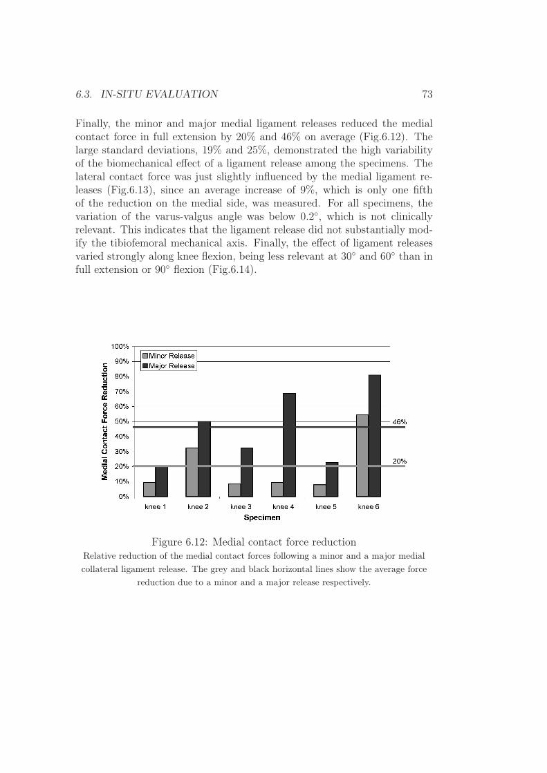
6.3. IN-SITU EVALUATION 73
Finally, the minor and major medial ligament releases reduced the medialcontact force in full extension by 20% and 46% on average (Fig.6.12). Thelarge standard deviations, 19% and 25%, demonstrated the high variabilityof the biomechanical effect of a ligament release among the specimens. Thelateral contact force was just slightly influenced by the medial ligament re-leases (Fig.6.13), since an average increase of 9%, which is only one fifthof the reduction on the medial side, was measured. For all specimens, thevariation of the varus-valgus angle was below 0.2◦, which is not clinicallyrelevant. This indicates that the ligament release did not substantially mod-ify the tibiofemoral mechanical axis. Finally, the effect of ligament releasesvaried strongly along knee flexion, being less relevant at 30◦ and 60◦ than infull extension or 90◦ flexion (Fig.6.14).
Figure 6.12: Medial contact force reductionRelative reduction of the medial contact forces following a minor and a major medialcollateral ligament release. The grey and black horizontal lines show the average force
reduction due to a minor and a major release respectively.
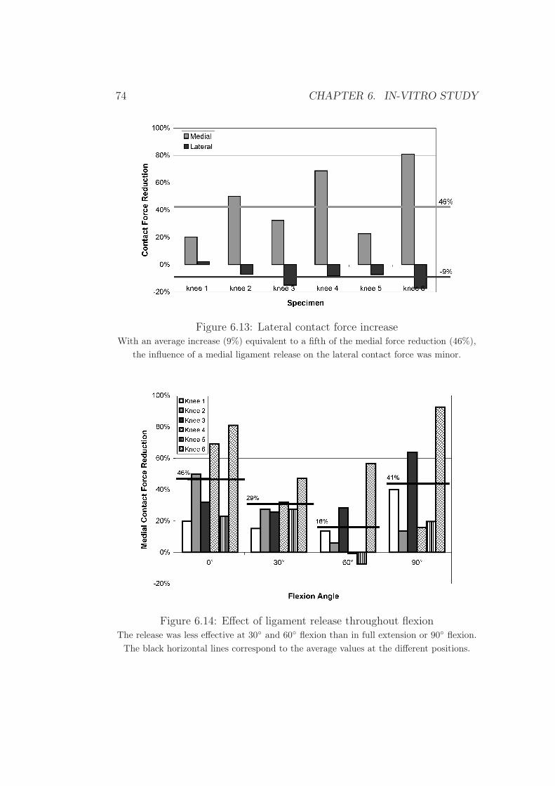
74 CHAPTER 6. IN-VITRO STUDY
Figure 6.13: Lateral contact force increaseWith an average increase (9%) equivalent to a fifth of the medial force reduction (46%),
the influence of a medial ligament release on the lateral contact force was minor.
Figure 6.14: Effect of ligament release throughout flexionThe release was less effective at 30◦ and 60◦ flexion than in full extension or 90◦ flexion.
The black horizontal lines correspond to the average values at the different positions.

6.3. IN-SITU EVALUATION 75
6.3.3 Discussion
The performance and the clinical advantages of the force-sensing device forimproved ligament balancing procedure in TKA was evaluated with six ca-daver knees and four different experiments: compression loading to validatethe device measurements, patella loading to demonstrate the advantage ofkeeping the patella in its anatomical place during the measurement, varus-valgus loading to compare the device measurements to the current surgicalapproach and finally ligament releasing to quantify its biomechanical effectin terms of forces.
The very good agreement between applied and measured tibiofemoral con-tact forces during the compression loading experiment proved the accuracyand reliability of the in-situ device measurements.
The advantage of having the patella in its anatomical place during the mea-surement was shown by the significant influence of the patellar eversion onthe mediolateral distribution of the condyle contact forces. One fourth ofthe patellar load was shifted to the lateral compartment with a patellar ev-ersion. Although the influence of patellar eversion on the mediolateral forcedistribution is intuitive, it is the first time according to the authors’ knowl-edge that the effect is quantified in terms of forces. Only one recent study[61] compared the influence of the patellar eversion and subluxation to thephysiological situation in terms of angular variation. With a given interar-ticular load of 150N for the medial and lateral side, the patellar eversionincreased the leg axis by 2.9◦ valgus. Although a quantitative comparisonto the present study is not possible, the measured effects are qualitativelyconsistent. Finally, the fact that the patella in its anatomical place alreadyinfluenced the mediolateral distribution of the contact forces could be due toa non-symmetrical contact area between the patella and the femoral trochleaor due to the medial incision of the knee joint.
The shape of the curves obtained during the varus-valgus loading experimentcan be biomechanically explained. When the joint opens after condyle lift-off,the lateral or medial collateral ligament bears a relevant part of the appliedload. Since this part is not measured by the device, it therefore appears asa drop in the slope. The difference of the slopes between the areas 1 and 3also demonstrates that the lateral and medial ligaments can have differentstiffness. The determination of the weight causing a medial or lateral condylelift-off allowed the comparison of the current surgical approach to assess theknee instability to the approach based on the measurement of the contact

76 CHAPTER 6. IN-VITRO STUDY
forces or varus-valgus moments. Overall, the three methods gave consistentresults. Weight-based imbalance assessment was equivalent to force-based,as expected by the simplified two-dimensional model. Moment-based imbal-ance assessment, which is assumed to be the optimal approach, showed atendency of lateral imbalance. This can be anatomically explained by thefact that the medial condyle is smaller than the lateral [62] and consequentlyhas its contact point closer to the center of the joint. It should also be notedthat this cadaver model does not take into account any arthritic deformities,which knees selected for TKA would have. Bone deformities can significantlyshift the condyle contact points and thereby further increase the differencebetween the force-based and moment-based imbalance assessment. In suchcases, measuring not only the contact forces but also the varus-valgus mo-ments is an undeniable advantage.
On average, the minor and major medial collateral ligament releases sub-stantially reduced the medial contact force (20% and 46% respectively). Thelarge variation among the specimens illustrates the difficulty of ligament re-lease. An intraoperative force monitoring during this delicate surgical actioncould provide further support to ensure an accurate, patient-specific adjust-ment of the ligament tensions. The increase of the lateral force after themajor medial ligament release was only a fifth of the decrease on the me-dial side. Consequently, in the case of a small ligament imbalance requiringonly a minor force reduction, the effect of the ligament release on the oppo-site side of the surgical action can be neglected. The ligament releases hadalso negligible effect on the tibiofemoral alignment. As ligament release canbe considered as a change of the ligament stiffness without modification ofthe ligament length, the medial and lateral knee gaps, and consequently thetibiofemoral alignment, are not affected. It is in opposition to the gap-basedapproach where the contact forces are kept constant with a distraction devicesuch as in the studies reported by Krackow et al. [63], Mihalko et al. [64]or Baldini et al. [65]. In these cases, diminishing the ligament stiffness witha ligament release alters the tibiofemoral gap due to constrain on the forceamplitude. Both methods, force-based and gap-based, are conceptually dif-ferent. While the former measures directly the contact forces determinant forthe component wear, the latter is limited by the complex force-displacementrelationship of ligaments, which moreover is not necessarily identical on themedial and lateral side. A well balanced distribution of medial and lateralcontact forces avoids overload of one compartment and thus premature wear.Finally, a variation of the effect of ligament releases along knee flexion wasobserved. A different arrangement of the ligament fibers in the different po-sitions could explain this variation. This again exemplifies the complexity of

6.3. IN-SITU EVALUATION 77
ligament balancing and the importance of an intraoperative force monitoring.
In conclusion, the device worked correctly under realistic conditions of use.In addition to the accurate imbalance assessment based on the measurementof forces and moments, important clinical advantages, such as the possibilityto keep the patella in its anatomical place during the measurement or thereal-time force monitoring during the delicate phase of ligament release, weredemonstrated. The proposed device has thus shown potential to improve theligament balancing procedure and the lifetime of TKA.

78 CHAPTER 6. IN-VITRO STUDY
Chapter 7
Clinical trials
7.1 Safety requirements
Before testing the device in-vivo, a risk analysis must be performed. Threekinds of risks can be identified:
1. Mechanical risks
• Damage to healthy tissues
• Rupture of the device
2. Chemical risks
• Contamination with toxic substances
• Infection
3. Electrical risks
• Electromagnetic disturbances
• Electric shocks
Since the shape of the device was designed to follow the contours of the tibialplateau, surrounding soft tissue is expected to be unaffected by insertion oruse of the device. Furthermore, the plasticity test showed that the devicestays in the elastic range with forces up to 1’500N. It is therefore expectedthat the force required to break the device is well over the maximum in-vivoload, thus making an in-situ rupture of the device impossible. Consequently,complications due to mechanical problems are very unlikely.
79

80 CHAPTER 7. CLINICAL TRIALS
All the metallic parts constituting the device are made of biocompatible stain-less steel or titanium. The wires have an insulation of teflon, a chemicallyinert material. All the connectors used are certified for medical applications.Therefore, the only possibility of chemical contamination comes from theexposed circuitry, piezoresistive sensors and soldering tabs. However, theparylene coating ensures a full chemical barrier and prevents toxic exposureto these parts. Finally, a standard sterilization procedure is adopted to min-imize risks of infection.
With a power supply of 5V DC, the device should not disturb any othersurgical device through electromagnetic interferences. Nevertheless, partic-ular attention must be paid to potential electric shocks. The device has tocomply with the general requirements of the standard for medical electricalequipment [66]. The two most important requirements are: a) a galvanicseparation that prevents direct connection between the electric network andthe patient and b) a patient leakage current that must not exceed 10µA innormal condition and 50µA in single fault condition. Although the parylenecoating provides a good electric isolation (3500V DC and 2500V AC), a spe-cial signal conditioning unit has been produced to further ensure the patientsafety in a fault condition (Fig.7.1).
Figure 7.1: Custom signal conditioning unit
The principle for the electric isolation of the patient is schematically ex-plained in Fig.7.2. The signal conditioning unit is powered by a power sup-
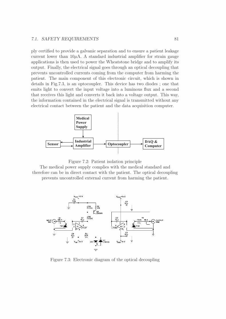
7.1. SAFETY REQUIREMENTS 81
ply certified to provide a galvanic separation and to ensure a patient leakagecurrent lower than 10µA. A standard industrial amplifier for strain gaugeapplications is then used to power the Wheatstone bridge and to amplify itsoutput. Finally, the electrical signal goes through an optical decoupling thatprevents uncontrolled currents coming from the computer from harming thepatient. The main component of this electronic circuit, which is shown indetails in Fig.7.3, is an optocoupler. This device has two diodes ; one thatemits light to convert the input voltage into a luminous flux and a secondthat receives this light and converts it back into a voltage output. This way,the information contained in the electrical signal is transmitted without anyelectrical contact between the patient and the data acquisition computer.
SensorIndustrialAmplifier
MedicalPowerSupply
OptocouplerDAQ &Computer
Figure 7.2: Patient isolation principleThe medical power supply complies with the medical standard and
therefore can be in direct contact with the patient. The optical decouplingprevents uncontrolled external current from harming the patient.
Figure 7.3: Electronic diagram of the optical decoupling

82 CHAPTER 7. CLINICAL TRIALS
7.2 Standard approach vs force-sensing device
Two clinical trials were carried out both to evaluate the device performancein a surgical environment and to compare the device-assisted to the stan-dard approaches under real conditions of use. To realize these objectives,two sets of measurements in full extension and in 90◦ flexion were carriedout, the first before the femoral cuts were performed and the second afterthe trial femoral component was placed. After the device insertion, spacersof different thicknesses were introduced to balance the ligament according tothe device measurements (Fig.7.4). Then, the device was removed and thesurgery proceeded in a standard way. The thickness of the resected condyleswas measured for the distal and posterior cuts. Once the trial femoral com-ponent was in place, the device was introduced a second time. Spacers wereused again to assess the remaining knee imbalance according to the devicemeasurements. The femoral cuts planned by the device measurements, thefemoral cuts performed on the basis of standard instrumentation as well asthe final imbalance assessment were then compared.
Patient A Patient BExtension Flexion Extension Flexion
Balanced knee 3mm 4mm 6mm 3mmFemoral cuts 3.5mm 1mm 6mm 2mmDifference -0.5mm 3mm 0mm 1mmFinal imbalance -1mm 2mm 0mm 0mm
Table 7.1: Mediolateral difference of the knee gapsA positive, negative sign corresponds to the medial, lateral side respectively.
The results are summarized in table 7.1. According to the device measure-ments, the knee of patient A could be balanced with a mediolateral differencein the knee gaps of 3mm in extension and 4mm in flexion. The femoral cutsperformed with a standard approach showed a gap difference of 3.5mm inextension and 1mm in flexion. Therefore, the device measurements and thestandard approach agreed in extension but not in flexion. However, thesurgeon also estimated at that point of the surgery that the knee was notcompletely balanced and that a ligament release was required. The kneeof patient B could be balanced with a mediolateral knee gap difference of6mm in extension and 3mm in flexion. The femoral cuts had a gap differenceof 6mm in extension and 2mm in flexion, showing a complete agreement

7.2. STANDARD APPROACH VS FORCE-SENSING DEVICE 83
(a) Overview of the operating room
(b) Introduction of spacers
Figure 7.4: Clinical trialSpacers are introduced to balance the knee according to the device measurements

84 CHAPTER 7. CLINICAL TRIALS
between the device-assisted and the standard approaches. The imbalanceassessment with the femoral component in place resulted in values similarto the difference between the device-planned femoral cuts and the femoralcuts effectively performed, thus demonstrating the consistency of the devicemeasurements throughout the surgery.
In addition to these measurements, five dynamic evaluations were performedduring knee flexion before the femoral resection. Fig.7.5 shows the variationin medial and lateral forces for patient A as the device spacers were set tobalance the knee at 90◦ flexion. The huge difference of force amplitude inflexion and in extension, and thereby the huge difference in balance, is inagreement with the well-known fact that tibiofemoral gaps ensuring a stableknee are not necessarily the same in flexion and in extension.
Figure 7.5: Flexion-extension of the knee
In conclusion, these in-vivo trials demonstrated that the device measure-ments are possible, meaningful and consistent with the surgeon’s perceptionin a clinical environment.

Chapter 8
Unicompartmental kneearthroplasty
8.1 Surgical procedureUnicompartmental Knee Arthroplasty (UKA) is a surgical procedure whichconsists in replacing either the medial or lateral knee compartment (Fig.8.1).This procedure is indicated when significant degenerative changes exist inonly one of the compartments and when the cruciate ligaments are intact.Candidate patients should not be obese, should have good preoperative rangeof motion (90◦ flexion), and a deformity below 15◦ [67]. These strict selec-tion criteria are responsible for the result that only 5-7% of arthritic kneejoints are treated with UKA. The theoretical advantages of UKA comparedto TKA are a preservation of the intact tissue and bone, a reduction in op-erating time as well as a better range of motion and improved gait.
UKA was introduced 30 years ago, but frequent and early failures at thattime made the treatment controversial. TKA with its encouraging long-termsuccess became the standard procedure. However, in the past few years, aresurgence of interest in the UKA has occurred, particularly with the intro-duction of minimally invasive techniques. With improved surgical proceduresand optimized prostheses, the long-term results with current UKA proceduresare now comparable to TKA ones, even though the demanding patient se-lection may influence the lifetime [68, 69, 70]. Moreover, a knee joint havingreceived a unicompartmental implant can later undergo a TKA, with min-imal loss of implant-supporting subchondral bone. Thus, at the point of aTKA, the UKA patient has gained the intervening time over an initial TKApatient.
85
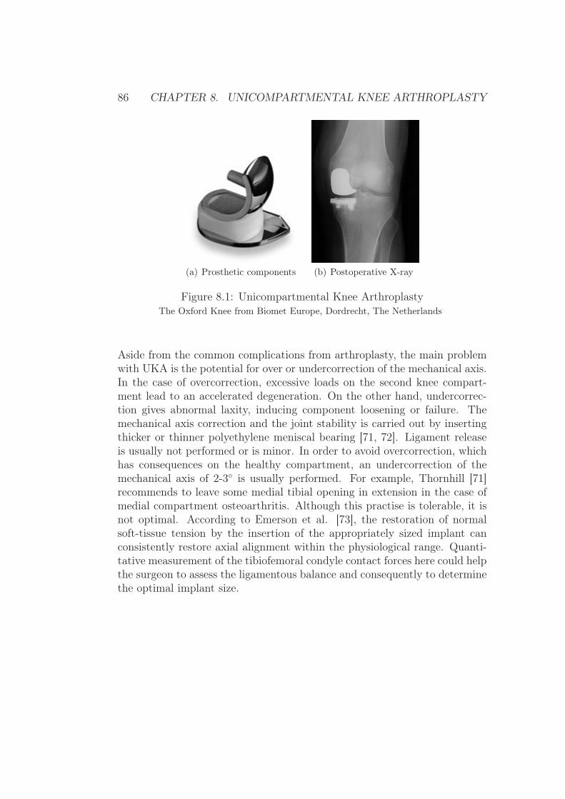
86 CHAPTER 8. UNICOMPARTMENTAL KNEE ARTHROPLASTY
(a) Prosthetic components (b) Postoperative X-ray
Figure 8.1: Unicompartmental Knee ArthroplastyThe Oxford Knee from Biomet Europe, Dordrecht, The Netherlands
Aside from the common complications from arthroplasty, the main problemwith UKA is the potential for over or undercorrection of the mechanical axis.In the case of overcorrection, excessive loads on the second knee compart-ment lead to an accelerated degeneration. On the other hand, undercorrec-tion gives abnormal laxity, inducing component loosening or failure. Themechanical axis correction and the joint stability is carried out by insertingthicker or thinner polyethylene meniscal bearing [71, 72]. Ligament releaseis usually not performed or is minor. In order to avoid overcorrection, whichhas consequences on the healthy compartment, an undercorrection of themechanical axis of 2-3◦ is usually performed. For example, Thornhill [71]recommends to leave some medial tibial opening in extension in the case ofmedial compartment osteoarthritis. Although this practise is tolerable, it isnot optimal. According to Emerson et al. [73], the restoration of normalsoft-tissue tension by the insertion of the appropriately sized implant canconsistently restore axial alignment within the physiological range. Quanti-tative measurement of the tibiofemoral condyle contact forces here could helpthe surgeon to assess the ligamentous balance and consequently to determinethe optimal implant size.

8.2. SOFT-TISSUE BALANCING ASSISTANCE FOR UKA 87
8.2 Soft-tissue balancing assistance for UKA
8.2.1 Concept
Since the contralateral knee compartment is not accessible during the surgery,only one sensitive plate can be used. This implies that only half of theparameters required to provide a quantitative evaluation of the knee balancecan be measured. Applying and measuring external varus-valgus loads onthe leg in addition to the one plate measurements can compensate for themissing information on the healthy side.
FMLFML
FMCFMC
FLLFLL
x
y
FextFext
d
FLCFLC
Figure 8.2: Knee joint experiencing external varus-valgus moments
The measurement principle is based on the same simplified planar model ofthe knee joint presented in section 3.1, except that an external force Fext isapplied at the distal part of the tibia at a distance d (Fig.8.2). The forcesFi, i={ML, MC, LC, LL} are the medial ligament, the medial contact, thelateral contact and the lateral ligament forces. To satisfy the equilibriumcondition, the sum of the moments must be zero.
dFext + xMLFML − xMCFMC + xLCFLC − xLLFLL = 0 , (8.1)

88 CHAPTER 8. UNICOMPARTMENTAL KNEE ARTHROPLASTY
where xi is the lever arm of the force Fi, i={ML, MC, LC, LL}. Byrenaming and regrouping the amplitude of the different moments, equation(8.1) can be rewritten as:
Mlig −MM +ML +Mext = 0 , (8.2)
where Mlig is the net varus-valgus moment of the collateral ligaments andMi, i={M , L, ext}, are the moment amplitudes of the medial, lateral andexternal forces respectively. The amplitude of the contact moments MM ,ML obviously depend on the external moment Mext. However, if bones areconsidered as rigid bodies and ligament as springs, the ligament forces andtherefore Mlig can be assumed constant as long as both condyles are in con-tact with the tibia. The tension in a spring-ligament would vary only whenthe joint starts to open, i.e. when one condyle lifts off. Therefore, the netvarus-valgus moment of the ligaments is given by:
Mlig = MM −ML −Mext 0 ≤Mext ≤M0ext , (8.3)
where M0ext corresponds to the moment creating a condyle lift-off. Since
this last equation is verifiedvalid for all the values of Mext comprised in thespecified range, it is true for the two border values:
Mlig = MM −ML for Mext = 0 (8.4)Mlig = MM −M0
ext for Mext = M0ext . (8.5)
Equation (8.4) shows that Mlig is equivalent to Mnet, the net varus-valgusmoment of the contact forces that characterizes the knee balance (c.f. section3.1) and equation (8.5) shows that it can be computed by measuring themedial and the external moments at the time of condyle lift-off:
Mnet = MM.
.
∣∣∣Mext=M0
ext
−M0ext . (8.6)
In practise, the medial moment MM is measured by the sensitive plate andthe external moment Mext can be computed from the measurement of theexternal force amplitude with a dynamometer and the lever arm with a ruler.The experimental issue is then to precisely determine the moment of condylelift-off without seeing the condyle. According to equation (8.2), a linearrelationship exists between the contact moment and the external varus-valgusmoment. However, the proportionality factors are not the same before andafter condyle lift-off since Mlig is constant and ML non-zero before, whereasMlig varies and ML is zero after lift-off. The specific external moment M0
ext
at the moment of lift-off can thus be determined by identifying the slopediscontinuity in the curve MM(Mext).

8.2. SOFT-TISSUE BALANCING ASSISTANCE FOR UKA 89
8.2.2 In-vitro feasibility study
The delicate point of the proposed method resides in the hypothesis thatMlig,the net varus-valgus moment of the collateral ligaments, does not vary beforecondyle lift-off. In practise, the knee joint is more complex than rigid bodieslinked with springs. For instance, the femoral cartilage can be compressedand behaves as a spring-like structure or the relative position between thefemur and tibia can slightly vary during loading, thus altering the ligamenttension. The goal of this section is therefore to quantify the deviation of themodel from the reality in order to estimate if the proposed approach couldbe used clinically.
If Mlig is constant, a partial derivative of equation (8.3) gives
∂
∂Mext
(MM −ML) = 1 . (8.7)
Consequently, plotting the net varus-valgus moment MM −ML in functionof the external moment Mext should show a linear relationship with a slopeof 1. To experimentally verify that point, the data acquired during thevarus-valgus loading experiment of the in-vitro study (c.f. section 6.3) wereused. For each specimen, the relationship was, as expected, highly linear(0.99≤ r2 ≤1.00), such as in the example showed in Fig.8.3. However, themeasured slopes ranged from 0.63 to 0.78, the average being 0.69 instead of1 (Table 8.1). This implies a relative error of the model of 30%, which isobviously not acceptable.
pilot knee 1 knee 2 knee 3 knee 4 knee 5 knee 6slope 0.78 0.72 0.61 0.74 0.66 0.69 0.63
Table 8.1: Slope of the ligament moment vs applied moment
The hypothesis of constant ligament forces before condyle lift-off is there-fore too strong. In order to improve the proposed approach, the variationof the net varus-valgus moment of the ligaments Mlig as a function of theexternal moment Mext must be taken into account. An estimate of this vari-ation may be derivable from an intraoperative measurement of the changeof the lengths LM , LL of the medial and lateral ligaments with the help ofa navigation system. Knowing this length variation, the force and therebythe moment variation can be estimated by using a generic or patient-specificligament stiffness (KM , KL). The latter can be determined by comparing

90 CHAPTER 8. UNICOMPARTMENTAL KNEE ARTHROPLASTY
Figure 8.3: Comparison of the contact moments and external moments
contact forces measured by the device and ligament lengths measured bythe navigation system in different external loading conditions. With theseparameters, the varation of the ligament moment can be computed as follows:
Mlig.
.
∣∣∣Mext=M0
ext
− Mlig.
.
∣∣∣Mext=0
= xMLKM∆LM − xLLKL∆LL ; (8.8)
and equation (8.6) can thus be corrected.
Mnet = MM.
.
∣∣∣Mext=M0
ext
−M0ext − (xMLKM∆LM − xLLKL∆LL) (8.9)
In conclusion, substituting the missing information of the healthy side byapplying known varus-valgus moments is not sufficient to provide precisestability assessment. Additional measurements, such as the variation of theligament length, are necessary.
Chapter 9
Conclusion and perspectives
This thesis addressed the issue of the measurement of musculoskeletal forcesduring orthopaedic surgeries through the development of a force-sensing de-vice for ligament balancing in Total Knee Arthroplasty (TKA). In additionto geometrical parameters given by the standard orthopaedic instrumenta-tion, the measurement of forces involved at the time of surgery can help inimproving the placement of implants and/or the adjustment of surroundingsoft-tissues to ensure a consistent procedure. During TKA, a good ligamentbalance must be achieved to ensure a stable and functional prosthetic kneejoint. Internal joint forces and moments are therefore of major importancebut are nowadays only qualitatively assessed with manipulation or basic in-strumentation.
In a first step, three possible designs for a force-sensing device for knee arthro-plasty were proposed and studied using finite element analysis. The optimaldesign consists of two sensitive plates, one for each condyle, a tibial baseplate, which is fixed by pins, and a set of lateral and medial spacers, whichallow the device thickness to be adapted to the patient-specific tibiofemoralgaps. The entire device fits inside the knee joint after the initial tibial cutwith the patella in its anatomical place. The ligament balance assessmentcan be carried out at the beginning of the surgery, thus offering the possi-bility to make a better plan for the femoral cuts and the femoral componentrotation. Thanks to the top spacer system, additional spacers having the topsurface congruent to femoral implants can be easily used to allow measure-ments and ligament adjustments with the trial components in place. Thus,the main stability assessment made at the beginning of the surgery enablesbetter planning of the femoral cuts, whereas the second at the end of thesurgery allows fine-tuning of the ligament balance and correcting eventualdeviations from the plan. Each sensitive plate contains three deformable
91
92 CHAPTER 9. CONCLUSION AND PERSPECTIVES
bridges instrumented with thick-film piezoresistive sensors. This three-pointmeasurement allows determining the amplitude and location of the load ap-plied on a sensitive plate. With these measurements, the net varus-valgusmoment, which has been identified as the biomechanical parameter charac-terizing the knee balance, can be computed. Laboratory experiments showedthat the device has an 0.5% full scale accuracy in the range 0-500N and a1.6N maximal measurement error in the range 0-100N, the expected activerange of use. Thus, the accuracy is adequate and the measurement principleand the device design validated.
In a second step, an in-vitro study demonstrated the proper in-situ func-tioning of the novel force-sensing device as well as its clinical advantages.For example, patellar eversion, necessary with standard approaches but notwith the proposed device, had a significant influence on the mediolateral dis-tribution of the contact forces: one fourth of the patellar load was shiftedto the lateral side. Besides the validation of the device design, this in-vitrostudy also addressed two biomechanical issues. The first is the absence ofstandard interpretation in biomechanical terms of what surgeons intuitivelycall ligament balancing. Contact pressure, contact forces, tibiofemoral gaps,angular asymmetry, etc., are parameters interchangeably used in literatureto describe the ligament balance. To identify which biomechanical parameterthe surgeon intraoperatively assesses, the current surgical approach (differ-ence of varus and valgus weights generating a condyle lift-off) was comparedtheoretically and experimentally to the measurement of contact forces ormoments. The weight-based method was similar to the force-based, whilethe moment-based, proposed as the optimal from the biomechanical pointof view, showed a slight lateral imbalance. Surgeons must then be awarethat knee stability before and after the insertion of the femoral componentmay differ even if the ligament forces do not. Instrumentation that bases theligament imbalance assessment on the measurement of contact forces andmoments should therefore be used during the planning of the femoral cuts.The second biomechanical issue is the lack or poor documentation of theeffect of ligament release, one of the most used surgical action to correct im-balance, in terms of knee joint forces. Medial contact forces measured afterminor and major medial collateral ligament releases were reduced by 20%and 46% in average. The high standard deviations, 19% and 25% respec-tively, demonstrated the high variability among specimens and therefore theneed of an intraoperative monitoring to ensure a patient-specific adjustmentof ligament tensions.
93
In a final step, two in-vivo trials confirmed that the device measurementsare possible, meaningful and consistent with the surgeon’s perception in aclinical environment.
The novel force-sensing device has therefore an appropriate design and per-forms correctly. In addition to the accurate imbalance assessment based onthe measurement of forces and moments, important clinical advantages, suchas the possibility to keep the patella in its anatomical place during the mea-surement or the real-time force monitoring in the delicate phase of ligamentrelease, were demonstrated. The proposed device has thus shown potentialto improve the ligament balancing procedure and the lifetime of TKA.
In order to further enhance the device, two ergonomic changes could be im-plemented. Firstly, the fixation mechanism serving to extend the sensitivearea could be replaced by a hinge mechanism at the extremity of the bridgepillars, which would extend the sensitive area to the whole plate while sup-pressing protuberant parts. Secondly, the data transfer to the computercould be improved by using a multiplexing or a telemetry to reduce or avoidwires. A prototypical telemetric system based on the principle of near-fieldmagnetic induction coupling, commonly used in RFID (Radio FrequencyIDentification) applications, was designed and tested by a research partner[47]. The technical feasibility was demonstrated but further work is neededto reduce the size of the electronics to be able to integrate it in the device. Inaddition to these ergonomic improvements, the functionality of the new in-strument can be extended by combining the device with a navigation system.Measuring simultaneously geometrical parameters, such as angles, lengths,axes, and mechanical such as forces and moments enables the use of com-plex computational knee models, which can act as assistive expert systems.The advantages that such a tool can offer was already perceived during thefeasibility study of the adaptation of the force-sensing device for unicompart-mental knee arthroplasty. Complete assistive expert systems, which intra-operatively provide an accurate measurement of geometrical and mechanicalparameters, a quantitative biomechanical interpretation and finally a preciseguidance to achieve the plan will undeniably become an essential tool in thenext generation of orthopaedic instrumentation.
The first in-vivo trials, which concluded the experimental phase of the the-sis, correspond to the starting point of large clinical studies. Thanks to thedeveloped force-sensing device several important biomechanical and clinicalissues can be addressed, such as the accuracy and repeatability of the sur-geon’s performance in soft tissue balancing ; the correlation between intra-
94 CHAPTER 9. CONCLUSION AND PERSPECTIVES
operative ligament imbalance, postoperative knee laxity and postoperativecomplications ; the lifetime of TKA performed with an assistive expert sys-tem compared to standard instrumentation. Up to now, all these importantquestions could not be studied quantitatively. The new proposed tool hastherefore a promising future in research, too.
As has been seen through the development of this force-sensing device forknee arthroplasty, intraoperative measurements of musculoskeletal forces isof major importance and can bring useful help during orthopaedic surgeries.Precise and objective assessment of biomechanical parameters is a valuablecomplement to the surgeon’s perception and the combination of smart surgi-cal instrumentation and human-specific performances should definitely leadto a significant benefit for the patient.

Appendix A
Some basics of solid mechanics
The purpose of this section is not to give an exhaustive course on solidmechanics, but simply to review and introduce the fundamental conceptsused in this thesis. More details on solid mechanics can be found in [10].
A.1 Elastic deformationTwo fundamental concepts in mechanics of materials are stress and strain.Stress is the intensity of a force per unit of area and is denoted by σ. As-suming that the stresses are uniformly distributed over a cross section of abody (Fig.A.1), the stress amplitude is expressed by
σ =P
A, (A.1)
where P is the axial force and A the area. By definition, stress is positivewhen the specimen is tensed and negative when it is compressed.
Figure A.1: Definition of stressStress σ is the intensity of a force P per unit of area A (picture taken from [10])
A straight bar becomes longer in axial tension and shorter in axial compres-sion. The resulting strain is denoted by ε and is defined as the ratio between
95
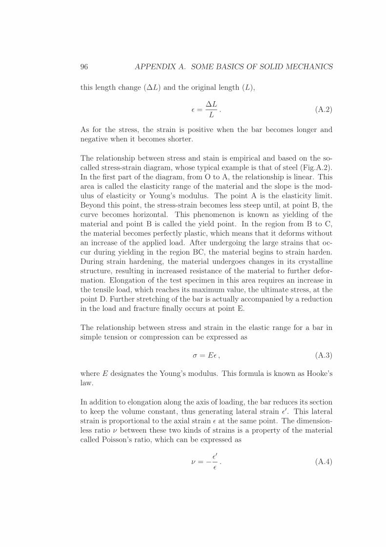
96 APPENDIX A. SOME BASICS OF SOLID MECHANICS
this length change (∆L) and the original length (L),
ε =∆L
L. (A.2)
As for the stress, the strain is positive when the bar becomes longer andnegative when it becomes shorter.
The relationship between stress and stain is empirical and based on the so-called stress-strain diagram, whose typical example is that of steel (Fig.A.2).In the first part of the diagram, from O to A, the relationship is linear. Thisarea is called the elasticity range of the material and the slope is the mod-ulus of elasticity or Young’s modulus. The point A is the elasticity limit.Beyond this point, the stress-strain becomes less steep until, at point B, thecurve becomes horizontal. This phenomenon is known as yielding of thematerial and point B is called the yield point. In the region from B to C,the material becomes perfectly plastic, which means that it deforms withoutan increase of the applied load. After undergoing the large strains that oc-cur during yielding in the region BC, the material begins to strain harden.During strain hardening, the material undergoes changes in its crystallinestructure, resulting in increased resistance of the material to further defor-mation. Elongation of the test specimen in this area requires an increase inthe tensile load, which reaches its maximum value, the ultimate stress, at thepoint D. Further stretching of the bar is actually accompanied by a reductionin the load and fracture finally occurs at point E.
The relationship between stress and strain in the elastic range for a bar insimple tension or compression can be expressed as
σ = Eε , (A.3)
where E designates the Young’s modulus. This formula is known as Hooke’slaw.
In addition to elongation along the axis of loading, the bar reduces its sectionto keep the volume constant, thus generating lateral strain ε′. This lateralstrain is proportional to the axial strain ε at the same point. The dimension-less ratio ν between these two kinds of strains is a property of the materialcalled Poisson’s ratio, which can be expressed as
ν = −ε′
ε. (A.4)

A.1. ELASTIC DEFORMATION 97
Figure A.2: Stress-strain diagramTypical structural steel in tension (picture taken from [10])
Taking the lateral strain into account, the triaxial Hooke’s law can be writtenas follows:
ε1 =1
E(σ1 − νσ2 − νσ3)
ε2 =1
E(σ2 − νσ1 − νσ3) (A.5)
ε3 =1
E(σ3 − νσ1 − νσ2) .
In addition to axial loads, tangential loads can act on a specimen’s surface.These loads generate shear stresses, which are denoted by τ . Contrary to ax-ial stress which tends to modify the length of a specimen, shear stress tendsto change its shape. The corresponding strain is not the relative length vari-ation anymore, but the angle of distortion γ (Fig.A.3).
The shear stress-strain diagram is similar in shape to the tension stress-straindiagram, although it differs in magnitude. A linear relationship, which iscalled the Hooke’s law in shear, also exists close to the origin.
τ = Gγ , (A.6)
where G is the shear modulus.

98 APPENDIX A. SOME BASICS OF SOLID MECHANICS
Figure A.3: Shear stressElement of material subjected to shearing stresses and strains, before and after
deformation (picture taken from [10])
Apparently, 12 shear stress components (2 per face for 6 faces) are requiredto completely describe the state of a general three-dimensional stress ele-ment. However, stresses occurring at opposing faces have opposite signs,thus reducing the number of significant components to 6. Moreover, in orderto satisfy static equilibrium, the shear stress components are related in thefollowing way:
τxy = τyx τyz = τzy τzx = τxz , (A.7)
where the first subscript is the coordinate normal to the element face and thesecond designates the axis parallel to the shear-stress component. Therefore,only 3 components are significant, or, in other words, independent. Thisleads to use the following three equations for a three-dimensional case ofpure shear:
τxy = Gγxy
τyz = Gγyz (A.8)τzx = Gγzx .
Although the normal and shear stresses were discussed separately, both cansimultaneously occur in a general load state. The set of equations (A.5)and (A.8) must therefore be used. Considering such a general case, it ispossible to demonstrate that the Young’s modulus, the shear modulus andthe Poisson’s ratio are related to each other by
G =E
2(1 + ν). (A.9)
Finally, note that all previous considerations are only valid for homogenousand isotropic material.

A.2. STRESSES IN BEAMS 99
A.2 Stresses in beams
An important and widely used mechanical structure in the domain of force-sensing devices is the bending beam. To establish the stress formula forbending beams, let’s consider the Fig.A.4, which presents the side view andthe cross section of a beam as well as its deformation resulting from bendingmoments.
Figure A.4: Deformation of beam in pure bendinga) side view, b) cross section, c) deformed beam (picture taken from [10])
When loads are applied to a beam, its longitudinal axis is deformed into acurve. The curvature (κ) is by definition the inverse of the radius of curvature(ρ), that is
κ =1
ρ. (A.10)

100 APPENDIX A. SOME BASICS OF SOLID MECHANICS
The neutral axis, the axis along which there is no stress, is represented bya dashed line. Since the distance dx between the planes containing crosssections mn and pq is part of this neutral axis which undergoes no strain, itremains the same before and after deformation, thus allowing us to write
ρdθ = dx , (A.11)
giving
κ =dθ
dx. (A.12)
On the other hand, a line ef at a distance y from the neutral axis becomesshorter or longer. Its original length is clearly dx and its length after defor-mation is
(ρ− y)dθ = dx− y
ρdx . (A.13)
The corresponding strain is therefore
εx =(dx− y
ρdx) − dx
dx= −y
ρ= −κρ , (A.14)
and stressσx = Eεx = −Eκy . (A.15)
To express the curvature in mechanical terms, the second equation of equilib-rium, which expresses the fact that the sum of the moments should be zero,has to be used. Considering a small part of the beam, the element of forceσxdA acting on an element dA is in the positive direction of the x axis whenσx is positive and inversely. An infinitesimal moment is therefore generated,
dM = −σxydA , (A.16)
thus giving by integration
M = −∫
A
σxydA = κE
∫A
y2dA = κEI , (A.17)
where I is the moment of inertia.
I =
∫A
y2dA (A.18)
The curvature can hence be expressed by
κ =1
ρ=M
EI. (A.19)

A.2. STRESSES IN BEAMS 101
Finally, by combining equations (A.15) and (A.19), the flexure formula isobtained:
σx = −My
I. (A.20)
This general expression gives the stress for a given cross-section in a specificplane, but designers are more interested in knowing the maximal stresses.These obviously occur at the top and bottom surface of the beam, when yis maximal. In order to give an analytical expression, two specific cases, arectangular and a circular beam, are now reviewed.
1. Let’s consider a rectangular beam with a width b and a height h. Ifa force is acting in its center, the maximal possible value for y is h/2.After integration, the moment of inertia is
I =bh3
12, (A.21)
and the maximal stress amplitude for a rectangular beam is
σx =6M
bh2(A.22)
2. Let’s consider a circular beam with a diameter d and a force actingin its center. The maximal value for y is d/2. After integration, themoment of inertia is
I =πd4
64. (A.23)
The maximal stress amplitude for a circular beam is
σx =32M
πd3(A.24)
Finally, note that this analysis is valid only for pure bending. Nonuniformbending, which corresponds to bending moment that is not constant alongthe beam, will produce distortion of the cross section. This distortion hasnot been taken into account in the previous development. However, detailedinvestigations show that the normal stresses calculated from the flexure for-mula are not significantly altered by the shear stresses. Thus, the theory ofpure bending for calculating normal stresses in beams subjected to nonuni-form bending can be justifiably used.
It has also to be reminded that this analysis does not take into accounteventual stress concentrations, making the theory inaccurate near the supportof the beam or close to a concentrated load.

102 APPENDIX A. SOME BASICS OF SOLID MECHANICS

Appendix B
Contact pressure and stresses
To evaluate if yielding of a body being in contact with other mechanical partswill occur, a two-step calculation has to be performed:
1. Assess the maximal contact pressure (B.1)
2. Determine if this maximal pressure leads to plastic yielding (B.2)
B.1 Hertzian theoryThis typical contact stress problem was solved by Hertz in 1881 for the firsttime. Even if the Hertzian theory is more than hundred years old, it is stilllargely used and has been numerous times validated.
The mathematical description that follows is from [74]. A more general ap-proach, which leads to the same final result, can be found in [75].
Let’s consider two bodies, which have spherical surfaces of radii R1, R2 atthe contact point (Fig.B.1). Without pressure between the bodies, the con-tact point is located in O. The distances from the plane tangent at O ofpoints such as M, N , at a very small distance r from the axes z1, z2, can berepresented with sufficient accuracy by the formula
z1 = R21 −
√R2
1 − r2 ∼= r2
2R1
(B.1)
and the respective distance between these points is
z1 + z2 =r2(R1 +R2)
2R1R2
. (B.2)
103

104 APPENDIX B. CONTACT PRESSURE AND STRESSES
Figure B.1: Two spheres in contact(picture taken from [74])
In the particular case of contact between a plane and a sphere (Fig.B.2),1/R1 = 0 and the mutual distance becomes
z1 + z2 =r2
2R2
. (B.3)
In the case of contact between a ball and a spherical seat (Fig.B.2), R1 isnegative and the mutual distance is
z2 − z1 =r2(R1 −R2)
2R1R2
. (B.4)
Figure B.2: Different contactsa) sphere on a plane, b) sphere in spherical socket (picture taken from [74])
Applying a load F on the spheres obviously leads to deformation. Thisgives a compliance δ corresponding to the movement in the vertical directionof points at a distance r from the loading point, such as M, N . If the

B.1. HERTZIAN THEORY 105
displacements at these points are w1, w2, then, for points inside the contactarea:
(z1 + w1) + (z2 + w3) = δ . (B.5)
With (B.2), this last equation can be written as:
w1 + w2 = δ − βr2 , (B.6)
where β = R1+R2
2R1R2.
Assuming that the radii of curvature R1, R2 are large in comparison to theradius of the contact surface, the result obtained for semi-infinite bodies in[74] can be applied: the displacement w1 of a point on the surface of contactof the lower ball is
w1 =1 − ν2
1
πE1︸ ︷︷ ︸=K1
∫∫P ds dψ = K1
∫∫P ds dψ , (B.7)
where ν1, E1 are the Poisson’s and Young’s modulus respectively and P thepressure. A similar expression can be written for the upper ball. Thus, (B.6)becomes
(K1 +K2)
∫∫P ds dψ = δ − βr2 . (B.8)
A satisfying assumption is that the distribution of pressure P over the contactarea is represented by the ordinates of an hemisphere of radius a, constructedon the surface of contact. If Pmax is the pressure at the center of the contactarea, then
Pmax = ka , (B.9)
where k is a constant factor representing the scale factor of our representationof the pressure distribution. After integration, (B.8) becomes
(K1 +K2)π2Pmax
4a(2a2 − r2) = δ − βr2 . (B.10)
Since this last equation has to be fulfilled for any value of r, it has to bevalid for r = 0 and r = a. Therefore, the following relationships exist forcompliance δ and the radius a of the surface of contact:
δ = (K1 +K2)Pmaxπ2a
2
a = (K1 +K2)Pmaxπ2
4β. (B.11)

106 APPENDIX B. CONTACT PRESSURE AND STRESSES
The value of the maximal pressure Pmax is obtained by equating the sumof the pressures over the contact area to the compressive force F . For thehemispherical pressure distribution, with Pmax/a being the pressure per unitof ordinates and 2/3πa3 the hemisphere volume, this gives
Pmax
a
2
3πa3 = F , (B.12)
from whichPmax =
3F
2πa2. (B.13)
The maximal pressure is thus 1.5 the average pressure of the contact area.
Finally, combining the expressions (B.11) and (B.13) gives the final result
a = 3
√3π
4F (K1 +K2)
R1R2
R1 +R2
δ = 3
√9π2
16F 2(K1 +K2)2
(R1 +R2)
R1R2
(B.14)
Pmax =1
π3
√6
π2
F
(K1 +K2)2
(R1 +R2)2
R21R
22
.
Note that by taking R1 infinite or negative, the equations are valid for a ballon a plane or in a socket. For a ball in a spherical seat, this gives:
Pmax =1
π3
√6
π2
F
(K1 +K2)2
(R1 −R2)2
R21R
22
.
B.2 Distortion-energy criterionAlthough the maximal pressure in the contact area can be calculated, a cri-teria to evaluate its effect on the material (elastic, plastic deformation orfailure) must be defined. In other words, the correlation between the expe-rienced stress and the yielding point or the ultimate tensile strength of thematerial should be determined. Unfortunately there is at present time nofundamental rationale for such correlation and the use of empirical relation-ships, which have been widely proved by experiments, is required. One of themost popular is surely the von Mises or distortion-energy criterion, which isdescribed below [76].

B.2. DISTORTION-ENERGY CRITERION 107
PostulateYielding will occur when the distortion-energy per unit volume equals thedistortion-energy per unit volume in a uniaxial tension specimen stressed toits yield strength.
The strain energy per unit volume is given by
U =1
2σ1ε1 +
1
2σ2ε2 +
1
2σ3ε3 , (B.15)
where σi, εi are the principal stress and strain components. An expression ofthe strain energy per unit volume in terms of stress only can be obtained byusing the stress-strain relationships,
ε1 =1
E(σ1 − νσ2 − νσ3)
ε2 =1
E(σ2 − νσ1 − νσ3) (B.16)
ε3 =1
E(σ3 − νσ1 − νσ2) ,
thus giving
U =1
2E
[σ2
1 + σ22 + σ2
3 − 2ν(σ1σ2 + σ2σ3 + σ3σ1)]. (B.17)
The principal stress components can be theoretically separated into two dif-ferent contributions: the hydrostatic and the distortional stresses (Fig.B.3).By definition, the hydrostatic stress is given by
σh =σ1 + σ2 + σ3
3. (B.18)
On one hand, the hydrostatic stresses cause a change only in volume, notin shape. A cube gets bigger in tension and smaller in compression, butremains a cube. On the other hand, distortional stresses act to deform ordistort the material element. There is no change in volume, only in shape.These stresses try to elongate or compress the material more in one directionthan in another and are responsible for yielding.

108 APPENDIX B. CONTACT PRESSURE AND STRESSES
Figure B.3: Hydrostatic and distortional stresses definition
The distortional strain energy is equal to the difference between the totalstrain energy and the hydrostatic strain energy.
Ud = U − Uh
=1
2E
[σ2
1 + σ22 + σ2
3 − 2ν(σ1σ2 + σ2σ3 + σ3σ1)]
−3
2
1 − 2ν
E
(σ1 + σ2 + σ3
3
)2
Ud =1 + ν
3E[σ2
1 + σ22 + σ2
3 − σ1σ2 − σ2σ3 − σ1σ3] (B.19)
Thus, the distortional strain energy depends only on the effective stress,ususally called the von Mises stress, defined by
σeff =√σ2
1 + σ22 + σ2
3 − σ1σ2 − σ2σ3 − σ1σ3 . (B.20)
In a uniaxial tension test (σ2 = σ3 = 0), this effective stress is equivalent tothe tension stress;
σeff = σ1 . (B.21)
Therefore, this effective stress is the parameter which should be comparedto the tensile strength of the material to determine if yielding may occur ornot.
B.3 Conclusion
From the two previous sections, the maximal contact pressure an the effec-tive stress that has to be compared to the tensile strength of material canbe computed. However, the link between both parameters still need to bedetermined. The maximum stresses of two spherical bodies in contact obvi-ously occur in the z axis. These are principal stresses and their expression is

B.3. CONCLUSION 109
given by [77]
σ1 = σ2 = −Pmax
(
1 − z
atan−1
(1za
))(1 + ν) − 1
2(1 +
(za
)2)
σ3 =−Pmax
1 +(
za
)2 . (B.22)
The corresponding shearing stress are given by
τxy =σ1 − σ2
2= 0
τxz = τyz =σ1 − σ3
2=σ2 − σ3
2. (B.23)
With these expressions, the curve representing the stresses per unit of Pmax
versus the depth in the z axis per unit of radius of contact area a can bedrawn (Fig.B.4).
Figure B.4: Principal, von Mises and shearing contact stress
Fig.B.4 shows that the maximal von Mises stress occur just below the surface,at a depth of 0.5a, and with an amplitude of
σmaxeff = 0.6Pmax . (B.24)

110 APPENDIX B. CONTACT PRESSURE AND STRESSES

Bibliography
[1] Nerlich A.G., Zink A., Szeimies U., Hagedorn H.G., Ancient EgyptianProsthesis of the Big Toe, Lancet, vol. 356, pp. 2176-2179 (2000)
[2] Breasted J.H., The Edwin Smith Surgical Papyrus, Chicago: The Uni-versity of Chicago Press (1930)
[3] Nolte L.P., Ganz R. (Editors), Computer Assisted OrthopaedicSurgery (CAOS), Bern: Hogrefe and Huber Publishers (1999)
[4] Dario P., Carrozza M.C., Marcacci M., D’Attanasio S., Magnami B.,Tonet O., Megali G., A Novel Mechatronic Tool for Computer-AssistedArthroscopy, IEEE T Inf Technol B, vol. 4(1), pp. 15-29 (2000)
[5] Allotta B., Belmonte F., Bosio L., Dario P., Study on a MechatronicTool for Drilling in the Osteosynthesis of Long Bones: Tool/BoneInteraction, Modeling and Experiments, Mechatronics, vol. 6(4), pp.447-459 (1996)
[6] Klöckner C., Rohlmann A., Bergmann G., Instrumented Forceps forMeasuring Tensile Forces in the Rod of VDS Implant During Correc-tion of Scoliosis, Biomed Tech, vol. 48(12), pp. 362-364 (2003)
[7] Marieb E.N., Human Anatomy and Physiology, 5th Ed., San Fran-cisco: Benjamin Cummings (2001)
[8] Pinskerova V., Iwaki H., Freeman M.A.R., The Shapes and RelativeMovements of the Femur and Tibia at the Knee, Orthopäde, vol.29(Suppl.1), pp. S3-S5(2000)
[9] Nordin M., Frankel V.H., Basic Biomechanics of the MusculoskeletalSystem, 2nd Ed., Philadelphia: Lea & Febriger (1989)
[10] Gere J.M., Mechanics of Material, 5th SI Ed., Cheltenham: NelsonThornes (2002)
111

112 BIBLIOGRAPHY
[11] Gluck T., Referat über die durch das moderne chirurgische Experimentgewonnenen positiven Resultate, betreffend die Naht und den Ersatzvon Defecten höherer Gewebe, sowie über die Verwertung resorbier-barer und lebendiger Tampons in der Chirurgie, Arch Klin Chir, vol41, pp. 187-239 (1890)
[12] Ranawat C.S., History of Total Knee Arthroplasty, J South OrthopAssoc, vol. 11(4), pp. 218-226 (2002)
[13] Kapandji I.A., The Physiology of the Joints, New York: ChurchillLivingstone (1976)
[14] Whiteside L.A., Soft Tissue Balancing, J Arthroplasty, vol.17(4),Suppl.1, pp. 23-27 (2002)
[15] Insall J., Ranawat C.S., Scott W.N., Walker P., Total Condylar KneeReplacement: Preliminary Report, Clin Orthop, vol. 120, pp. 149-154(1976)
[16] Harner C.D., Vince K.G., Fu F.H., Techniques in Knee Surgery,Philadelphia: Lippincott Williams & Wilkins (2001)
[17] Rathjen K.W., Surgical Treatment. Total Knee Arthroplasty, Am JKnee Surg, vol. 11(1), pp. 58-63 (1998)
[18] Rand J. A., Trousdale R. T., Ilstrup D. M., Harmsen W. S., Factorsaffecting the durability of primary total knee prostheses, J Bone JointSurg Am, vol. 85(2), pp. 259-265(2003)
[19] Lotke P.A., Ecker M.L., Influence of Positioning of Prosthesis in TotalKnee Replacement, J Bone Joint Surg Am, vol. 59(1), pp. 77-79 (1977)
[20] Freeman M.A., Todd R.C., Bamert P., Day W.H., ICLH Arthroplastyof the Knee: 1968–1977, J Bone Joint Surg Br, vol. 60-B(3), pp. 339-344 (1978)
[21] Insall J.N., Binazzi R., Soudry M., Mestriner L.A., Total Knee Arthro-plasty, Clin Orthop, vol. 192, pp.13-22 (1985)
[22] Dorr L.D., Boiardo R.A., Technical Considerations in Total KneeArthroplasty, Clin Orthop, vol. 205, pp. 5-11 (1986)
[23] Moreland J.R., Mechanisms of Failure in Total Knee Arthroplasty,Clin Orthop, vol. 226, pp. 49-64 (1988)

BIBLIOGRAPHY 113
[24] Windsor R.E., Scuderi G.R., Moran M.C., Insall J.N., Mechanisms ofFailure of the Femoral and Tibial Components in Total Knee Arthro-plasty, Clin Orthop, vol. 248, pp. 15-19 (1989)
[25] Teeny S.M., Krackow K.A., Hungerford D.S., Jones M., Primary To-tal Knee Arthroplasty in Patients with Severe Varus Deformity. AComparative Study., Clin Orthop, vol. 273, pp. 19-31 (1991)
[26] Fehring T.K., Valadie A.L., Knee Instability after Total Knee Arthro-plasty, Clin Orthop, vol. 299, pp. 157-162 (1994)
[27] Karachalios T., Sarangi P.P., Newman J.H., Severe Varus and ValgusDeformities Treated by Total Knee Arthroplasty, J Bone Joint SurgBr, vol. 76(6), pp. 938-942 (1994)
[28] Matsuda S., Miura H., Nagamine R., Urabe K., Harimaya K., Mat-sunobu T., Iwamoto Y., Changes in Knee Alignment after Total KneeArthroplasty, J Arthroplasty, vol.14(5), pp.566-570 (1999)
[29] Langlotz F., Nolte L.-P., Computer-Assisted Orthopaedic Surgery:From Theory to the Operating Room, Tech Orthop, vol. 18, pp. 140-148, 2003.
[30] Jenny J. Y., Boeri C., Computer-assisted implantation of total kneeprostheses: a case-control comparative study with classical instrumen-tation, Comp Aided Surg, vol. 6(4), pp. 217-220 (2001)
[31] Kunz M., Der intraoperative Einsatz von bildfreien, comput-ergestützten Systemen in der Kniechirurgie zur Wiederherstellung dernatürlichen Kinematik, Ph.D. Thesis, Maurice E. Müller-Institut fürBiomechanik, University of Bern, Switzerland (2003)
[32] Stulberg S. D., How accurate is current TKR instrumentation, ClinOrthop, vol. 416, pp. 177-184 (2003)
[33] Decking R., Markmann Y., Fuchs J., Puhl W., Scharf H.P., Leg axisafter computer-navigated total knee arthroplasty, J Arthroplasty, vol.20(3), pp. 282-288 (2005)
[34] Haaker R.G., Stockheim M., Kamp M., Proff G., Breitenfelder J.,Ottersbach A., Computer-assisted navigation increases precision ofcomponent placement in total knee arthroplasty, Clin Orthop, vol. 433,pp. 152-159 (2005)

114 BIBLIOGRAPHY
[35] Attfield S. F., Warren-Forward M. , Wilton T., Sambatakakis A.,Measurement of soft tissue imbalance in total knee arthroplasty usingelectronic instrumentation, Med Eng Phys, vol. 16(6), pp. 501-505(1994)
[36] Wallace A. L., Harris M. L., Walsch W. R., Bruce W. J., Intraoperativeassessment of tibiofemoral contact stresses in total knee arthroplasty,J Arthroplasty, vol. 13(8), pp. 923-927 (1996)
[37] Wasielewski R.C., Galat D.D., Komistek R.D., An intraoperativepressure-measuring device used in total knee arthroplasties and itskinematics correlations, Clin Orthop, vol. 427, pp. 171-178 (2004)
[38] Wasielewski R.C., Galat D.D., Komistek R.D., Correlation of com-partment pressure data from an intraoperative sensing device withpostoperative fluoroscopic kinematic results in TKA patients, JBiomech, vol. 38(2), pp. 333-339 (2005)
[39] Takahashi T., Wada Y., Yamamoto H., Soft-tissue balancing with pres-sure distribution during total knee arthroplasty, J Bone Joint Surg, vol.79(2), pp. 235-239 (1997)
[40] D’Lima D. D., Patil S., Steklov N., Colwell C. W., In vitro mea-surement of dynamic soft-tissue balance during total knee arthroplastywith an instrumented tibial prosthesis, in Trans. 50th annual meetingof Orthopaedic Research Society, San Francisco, pp. 301 (2004)
[41] Morris B. A., D’Lima D. D., Slamin J., Kovacevic N., Arms S. W.,Townsend C. P., Colwell C. W., E-Knee: evolution of the electronicknee prosthesis, J Bone Joint Surg Am, vol. 83 Suppl 2(Pt 1), pp.62-66(2001)
[42] Kauffman K. R., Kovacevic N., Irby S. E., Colwell C. W., Instru-mented implant for measuring tibiofemoral forces, J Biomech, vol.29(5), pp. 667-671 (1996)
[43] Davy D. T., Kotzar G., Berilla J., Brown R.H., Telemetrized or-thopaedic implant work at Case Western Reserve University, in Im-plantable Telemetry in Orthopaedics, Bergmann G., Graichen F.,Rohlmann A., Ed. Berlin: Forschungsvermittlung der Freien Univ.,pp. 205-219 (1990)
[44] Winemaker M.J., Perfect balance in total knee arthroplasty: the elu-sive compromise, J Arthroplasty, vol. 17(1), pp. 2-10 (2002)
BIBLIOGRAPHY 115
[45] Ritschl P., Machacek F. Jr., Fuiko R., Computer assisted ligamentbalancing in TKR using the Galileo system, 3rd Annual Meeting ofCAOS-International Proceedings, pp. 304-305, June 2003
[46] Marmignon C., Leimnei A., Cinquin P., Robotized distraction devicefor knee replacement, Proceedings of Computer Assisted Radiologyand Surgery, pp. 638-643 (2004)
[47] Kauert D., A wireless telemetric system in total knee arthropplasty,Diploma Thesis, Division of Microtechnology, University of AppliedSciences, Biel, Switzerland (2004)
[48] Grimaldi C., Ryser P., Straessler S., Gauge factor enhancement drivenby heterogeneity in thick-film resistors, J Appl Phys, vol. 90(1), pp.322-27 (2001)
[49] Grimaldi C., Ryser P., Stässler S., Piezoresistive anisotropy of thick-film resistors, J Eur Ceram Soc, vol. 24(6), pp. 1893-96 (1992)
[50] Prudenziati M., Morten B., The state of the art in thick-film sensors,Microelectr J , vol. 23, pp. 133-41 (1992)
[51] White N.M., Turner J.D., Thick-film sensors: past, present and future,Meas Sci Technol, vol. 8, pp. 1-20 (1997)
[52] White N.M., Study of the piezoresistive effect in thick-film resistorsand its application to load transduction, Ph.D. thesis, Faculty of Engi-neering & Applied Science, University of Southampton, United King-dom (1988)
[53] White N.M., Brignell J.E., A planar thick-film load cell, Sensor Actu-ator A, vol. 26, pp. 313-19 (1991)
[54] Arshak K.I., Ansari F., Collins D., Analysis of thick film strain resis-tors on stainless steel and ceramic substrates, Int J Electronics, vol.76(2), pp. 365-376 (1994)
[55] Fraigi L., Lupi D., Malatto L., A thick-film pressure for cars propelledby natural gas, Sensor Actuator A, vol. 42, pp. 439-41 (1994)
[56] Jacq C., Maeder Th., Ryser P., High-strain response of piezoresistivethick-film resistors on titanium alloy substrates, J Eur Ceram Soc,Vol. 24, pp. 1897-1900 (2004)

116 BIBLIOGRAPHY
[57] Hrovat M., Smetana W., Belavic D., Homolka H., Reicher R., ZarnikM.S., An investigation of thick-film materials on steel substrates forpossible sensor applications, Proceedings, IMAPS Poland, Polanczyk,Poland, pp. 199-202 (2001)
[58] Hrovat M., Belavič D., Benčan A., Bernard J., Holc J., Cilenšek J.,Smetana W., Homolkac H., Reicher R., Golonka L., Dziedzic A., KitaJ., Thick-film resistors on various substrates as sensing elements forstrain-gauge applications, Sensor Actuator A, Vol. 107, pp. 261-72(2003)
[59] Maeder T., Grimaldi C., Ryser P., Properties of thick-film resistors ondielectric and metal substrates for piezoresistive sensors, Proceedings,IMAPS Poland, Podlesice, pp. 219-222 (2003)
[60] Dürselen L., Claes L., Kiefer H., The influence of muscle forces andexternal loads on cruciate ligament strain, The American Journal ofSports Medicine, Vol. 19, pp. 381-383 (1995)
[61] Lüring C., Hüfner T., Kendoff D., Perlick L., Bäthis H., Grifka J.,Influence of everted and subluxed patella in ligament balancing, Pro-ceedings, CAOS-International, Helsinki, Finland, pp. 289-292 (2005)
[62] Röstlund T., Carlsson L., Albrektsson B., Albrektsson T., Morpho-metrical studies of human femoral condyles, Journal of BiomedicalEngineering, Vol. 11, pp. 442-448 (1989)
[63] Krackow K.A., Mihalko W.M., The effect of medial release on flexionand extension gaps in cadaveric knees, The American Journal of KneeSurgery, Vol. 12, pp. 222-228 (1999)
[64] Mihalko W.M., Whiteside L.A., Krackow K.A., Comparison ofligament-balancing techniques during total knee arthroplasty, TheJournal of Bone and Joint Surgery, Vol. 85-A (Suppl. 4), pp. 132-135(2003)
[65] Baldini A., Scuderi G.R., Aglietti P., Chalnick D., Insall J.N., Flexion-extension gap changes during total knee arthroplasty, The Journal ofKnee Surgery, Vol. 17(2), pp. 69-72 (2004)
[66] International Electrotechnical Commission, International standard onmedical electrical equipment, IEC 60601-1, Geneva, Switzerland

BIBLIOGRAPHY 117
[67] Kozinn S.C., Scott R., Current concepts review: unicondylar kneearthroplasty, J Bone JOint Surg Am, vol. 71-A, pp. 145-50 (1989)
[68] Murray D.W., Goodfellow J.W., O’Connor J.J., The Oxford medialunicompartmental arthroplasty: a ten-year survival study, J BoneJoint Surg Br, vol. 80-B(6), pp. 983-9 (1998)
[69] Berger R.A., Nedeff D.D., Barden R.M., Sheinkop M.M., Jacobs J.J.,Rosenberg A.G., Galante J.O., Unicompartmental knee arthroplasty:clinical experience at 6- to 10-year followup, Clin Orthop, vol. 367,pp. 50-60 (1999)
[70] Vince K.G., Cyran L.T., Unicompartmental knee arthroplasty: Newindications, more complications?, J Arthroplasty, vol. 19(4) Suppl 1,pp. 9-16 (2004)
[71] Thornhill T.S., Unicompartmental knee arthroplasty, Clin Orthop, vol.205, pp. 121-31 (1986)
[72] Goodfellow J.W., Kershaw C.J., D’a Benson M.K., O’Connor J.J.,The Oxford knee for unicompartmental osteoarthritis, J Bone JointSurg Br, vol. 70-B(5), pp. 692-701, (1988)
[73] Emerson R.H. Jr, Head W.C., Peters P.C. Jr, Soft-tissue balanceand alignement in medial unicompartmental knee arthroplasty, J BoneJoint Surg Br, vol. 74-B(6), pp. 807-10 (1992)
[74] Timoshenko S.P., Goodier J.N., Theory of Elasticity, Auckland: Mc-Graw Hill (1988)
[75] Whitehouse D.J., Handbook of Surface Metrology, Bristol: Instituteof Physics Publishing (1994)
[76] Dieter G.E., Mechanical Metallurgy, London: McGraw Hill (1988)
[77] Shigley J.E., Mischke C.R., Mechanical Engineering Design, 5th Ed.,New York: McGraw Hill (1989)

118 BIBLIOGRAPHY

Curriculum Vitae
Name DENIS CROTTETDate of birth 12th August 1976, Fribourg, SwitzerlandNationality SwissMarital status Married
EDUCATION
2001-2005 Ph.D. in Biomedical Engineering & MicrotechniqueLaboratoire de Systèmes Robotiques, EPF Lausanne
1996-2001 M.Sc. in PhysicsDepartment of Physics, EPF Lausanne
1992-1996 High school, scientific sectionCollège Sainte-Croix, Fribourg
PROFESSIONNAL EXPERIENCES/PROJECTS
2001-2005 MEM Research Center for Orthopaedic Surgery, Bern"A FORCE-SENSING DEVICE FOR TKA": Development of aforce-sensing device to help the surgeon balance soft-tissues duringtotal knee arthroplasty.
2000-2001 Institut de Physique Expérimentale, EPF Lausanne"ANTENNAE COMPATIBLE FOR ENDOVASCULAR MRI":Development of an endovascular antenna able to provide high reso-lution magnetic resonance images for diagnosis of vascular diseases.
1999-2000 CFG Microelectronics, MorgesSummer internship followed by a part-time work"ORGANIC LIGHT EMITTING DIODES": Identification of thelifetime-limiting parameters of organic light emitting diodes.
119

120
JOURNAL ARTICLES
1. Crottet D., Kowal J., Sarfert S.A., Maeder T., Bleuler H., Nolte L.P.,Dürselen L., Ligament Balancing in TKA: Evaluation of a Force-SensingDevice and the Influence of Patellar Eversion and Ligament Release,Journal of Biomechanics, submitted
2. Crottet D., Maeder T., Fritschy D., Bleuler H., Nolte L.P., PappasI.P., Development of a Force Amplitude- and Location-Sensing DeviceDesigned to Improve the Ligament Balancing Procedure in TKA, IEEETransactions on Biomedical Engineering, vol. 52(9), pp. 1609-1611,September 2005
3. Crottet D., Meuli R., Wicky S., van der Klink J.J., Reciprocity andSensitivity of Opposed-Solenoid Endovascular MRI Probes, Journal ofMagnetic Resonance, vol. 159, pp. 219-225, December 2002
CONFERENCE ABSTRACTS
1. Crottet D., Kowal J., Sarfert S.A., Bleuler H., Nolte L.P., DürselenL., In-Situ Evaluation of a Force-Measuring Device for Assistance inLigament Balancing during Knee Arthroplasty, 5th Annual Meeting ofthe International Society for Computer Aided Orthopaedic Surgery,147-8, Helsinki, Finland, June 2005
2. Crottet D., Maeder T., Sarfert S., Fritschy D., Bleuler H., Nolte L.P.,Pappas I.P., In-vitro Evaluation of a Force-Sensing Device for LigamentBalancing in TKA, 51st Annual Meeting of the Orthopaedic ResearchSociety, Washington, USA, February 2005
3. Crottet D., Maeder T., Fritschy D., Bleuler H., Nolte L.P., PappasI.P., In-vitro Validation of a Device Measuring the Tibio-femoral Con-tact Forces and Moments for Assistance during Ligament Balancing inTKA, 17th Annual Symposium of the International Society for Tech-nology in Arthroplasty, Rome, Italy, September 2004
4. Crottet D., Maeder T., Fritschy D., Bleuler H., Nolte L.P., Pappas I.P.,A Force-Sensing Device for Ligament Balancing in Total Knee Arthro-plasty, 4th Annual Meeting of the International Society for ComputerAided Orthopaedic Surgery, 147-8, Chicago, USA, June 2004

121
PATENT
1. D. Crottet, I.P. Pappas, T. Maeder, C. Jacq, H. Bleuler, Device forMeasuring Tibio-Femoral Force Amplitudes and Force Locations in To-tal Knee Arthroplasty, international patent application, PCT/CH04/000361, June 2004.
AWARDS
1. 2005 Research Award of the Swiss Society of Biomedical Engineering
2. 2004 Best Poster Award of the 4th Annual Meeting of the InternationalSociety for Computer Aided Orthopaedic Surgery