A Feasibility Study of Bridge Deck Deicing Using Geothermal Energy · A Feasibility Study of Bridge...
120
A Feasibility Study of Bridge Deck Deicing Using Geothermal Energy Morgan State University The Pennsylvania State University University of Maryland University of Virginia Virginia Polytechnic Institute & State University West Virginia University The Pennsylvania State University The Thomas D. Larson Pennsylvania Transportation Institute Transportation Research Building University Park, PA 16802-4710 Phone: 814-865-1891 Fax: 814-863-3707 www.mautc.psu.edu
Transcript of A Feasibility Study of Bridge Deck Deicing Using Geothermal Energy · A Feasibility Study of Bridge...

A Feasibility Study of Bridge Deck Deicing Using Geothermal Energy
Morgan State University The Pennsylvania State University
University of Maryland University of Virginia
Virginia Polytechnic Institute & State University West Virginia University
The Pennsylvania State University The Thomas D. Larson Pennsylvania Transportation Institute
Transportation Research Building University Park, PA 16802-4710 Phone: 814-865-1891 Fax: 814-863-3707
www.mautc.psu.edu

i
1. Report No.
MAUTC-2013-02
2. Government Accession No. 3. Recipient’s Catalog No.
4. Title and Subtitle
A Feasibility Study of Bridge Deck Deicing using Geothermal Energy
5. Report Date
April 28, 2015
6. Performing Organization Code
7. Author(s)
Omid Ghasemi-Fare, G. Allen Bowers, Cory A. Kramer, Tolga Y. Ozudogru, Prasenjit Basu, C. Guney Olgun, Tanyel Bulbul, Melis Sutman
8. Performing Organization Report No.
9. Performing Organization Name and Address
PI: Prasenjit Basu, Ph.D. The Pennsylvania State University Larson Transportation Institute 201 Transportation Research Building University Park, PA 16802 Co-PI: C. Guney Olgun, Ph.D. Virginia Polytechnic Institute and State University Department of Civil and Environmental Engineering 200 Patton Hall 750 Drillfield Drive Blacksburg, VA 24061
10. Work Unit No. (TRAIS)
11. Contract or Grant No.
DTRT12-G-UTC03
12. Sponsoring Agency Name and Address
US Department of Transportation Research & Innovative Technology Admin UTC Program, RDT-30 1200 New Jersey Ave., SE Washington, DC 20590
13. Type of Report and Period Covered
Final 1/1/2013-7/31/2014
14. Sponsoring Agency Code
15. Supplementary Notes
16. Abstract
In this study, we investigated the feasibility of a ground-coupled system that utilizes heat energy harvested from the ground for
deicing of bridge decks. Heat exchange is performed using circulation loops integrated into the deep foundations supporting the
bridge or embedded within the approach embankment. The warm fluid extracted from the ground is circulated through a tubing
system embedded within reinforced concrete bridge deck to keep the deck temperature above the freezing point. A circulation pump
that requires a minimal amount of power is used for fluid circulation. This is different from ground-source heat pump systems used
for heating and cooling of buildings. In this study, a proof-of-concept testing is developed to investigate the operational principles
and key design parameters. Experiments were performed on a model-scale instrumented bridge deck and model heat-exchanger
piles to investigate heat transfer within different components of the ground-coupled bridge deck system. Heat transfer within ground
and concrete bridge deck is quantified through numerical simulations under a variety of design and operational conditions.
Experimental and numerical studies performed both at Penn State and Virginia Tech campuses demonstrate that this technology
has a significant potential in reducing the use of salts and deicing chemicals. The knowledge and experience gained from this
research will guide future research on real-life implementation of the proposed alternative bridge deck deicing method and will
eventually help the concept to grow as a ready-to-use technology. Consequently, it will be possible to reduce bridge deck
deterioration and offset the detrimental effects and environmental hazards caused by these chemicals.
17. Key Words: Geothermal energy; Deicing technology; Concrete
bridges; Heat transfer analysis; Heat exchanger piles
18. Distribution Statement
No restrictions. This document is available from the National Technical Information Service, Springfield, VA 22161
19. Security Classif. (of this report)
Unclassified
20. Security Classif. (of this page)
Unclassified
21. No. of Pages
110
22. Price

ii
Table of Contents
1. Problem Statement .................................................................................................................. 1
2. Review of Existing Literature ................................................................................................. 2
2.1 Geothermal bridge deck deicing case histories ................................................................ 2
2.2 Numerical studies of bridge deck deicing ........................................................................ 3
3. Laboratory-scale tests on a model heat exchanger pile .......................................................... 4
3.1 Scale Effect ...................................................................................................................... 4
3.2 Test setup.......................................................................................................................... 5
3.2.1 Sand bed saturation ................................................................................................... 7
3.2.2 Model geothermal pile .............................................................................................. 7
3.3 Material Characterization ................................................................................................. 9
3.3.1 Sieve Analysis ........................................................................................................... 9
3.3.2 Mechanical properties of Ottawa sand .................................................................... 10
3.3.3 Scanning electron microscope (SEM) .................................................................... 11
3.3.4 Thermal conductivity .............................................................................................. 13
3.3.5 Hydraulic conductivity............................................................................................ 17
3.4 Concrete model pile ....................................................................................................... 18
3.5 Instrumentation and data acquisition.............................................................................. 19
3.5.1 Thermocouples ........................................................................................................ 19
3.5.2 Load cell and displacement sensor ......................................................................... 20
3.5.3 Labview code .......................................................................................................... 21
3.6 Results ............................................................................................................................ 22
3.6.1 Thermal performance .............................................................................................. 22
3.7 Observations from thermal tests ..................................................................................... 32
4. Laboratory-scale tests on bridge deck (concrete slabs) ........................................................ 33
4.1 Field test setup and construction .................................................................................... 33
4.2 Experimental tests and results ........................................................................................ 35
4.2.1 Bridge deck heating ................................................................................................ 35
4.2.2 Ground response to bridge deck heating ................................................................. 38
4.3 Ground Thermal Recharge ............................................................................................. 41
5. Structural performance evaluation of a concrete bridge deck overlay ................................. 44

iii
5.1 Current design methodology .......................................................................................... 44
5.2 Observed temperature gradients from experimental heating tests ................................. 45
5.3 Observed temperature gradients from experimental bridge deck cooling tests ............. 47
5.4 Conclusions and future analysis considerations ............................................................. 48
6. Finite difference analysis of heat exchange through geothermal piles ................................. 50
6.1 Annular cylinder model .................................................................................................. 50
6.1.1 Validation of the developed finite difference code ................................................. 51
6.1.2 Analysis results ....................................................................................................... 52
6.1.3 Effect of operational parameters ............................................................................. 55
6.1.4 Variation of heat flux and fluid temperature ........................................................... 57
6.2 U-tube model .................................................................................................................. 59
6.2.1 Finite difference formulation .................................................................................. 61
6.2.2 Stability condition ................................................................................................... 63
6.2.3 Verification ............................................................................................................. 63
6.2.4 Comparison with published field test data .............................................................. 66
6.2.5 Temperature Difference T between Inlet and Outlet Points ................................. 68
6.2.6 Geothermal Power Output ...................................................................................... 71
6.2.7 Closed-form expression to predict power output .................................................... 73
6.3 Identification of sensitive uncertain parameters............................................................. 74
6.4 Summary and conclusion ............................................................................................... 76
7. Finite element analysis of heat exchange through geothermal piles..................................... 77
7.1 Model development ........................................................................................................ 77
7.2 Modifications ................................................................................................................. 79
7.3 Model Performance ........................................................................................................ 81
8. Finite element analysis of bridge deck deicing ..................................................................... 83
8.1 Model development ........................................................................................................ 85
8.1.1 The governing physics included in the model ........................................................ 85
8.1.2 Geometry, material properties, and domain discretization ..................................... 86
8.2 Parametric analysis methodology................................................................................... 87
8.3 Results ............................................................................................................................ 88
8.4 Conclusions .................................................................................................................... 96
9. Cost analysis ......................................................................................................................... 97
9.1 Introduction to life cycle analysis (LCA) ....................................................................... 97

iv
9.2 Steps of a LCA ............................................................................................................... 97
9.3 The life cycle of deicing salt (Calcium Chloride) .......................................................... 99
9.4 Cradle-to-Gate life cycle assessment of deicing salt (Calcium Chloride CaCl2) ......... 100
10. List of references.............................................................................................................. 104

v
List of Figures
Figure 3-1 Setup for model-scale tests performed at PSU: (a) soil tank (b) top view of the model
geothermal pile embedded in the sand bed............................................................................ 5
Figure 3-2 Sand pluviation system using #6, #10, and #12 sieves ................................................. 6
Figure 3-3 Relative density calibration curve ................................................................................. 7
Figure 3-4 Vertical and horizontal cross-sections of the test pile ................................................... 8
Figure 3-5 Particle size distribution curve for F50 Ottawa sand .................................................... 9
Figure 3-6 Particle size distribution for crushed limestone .......................................................... 10
Figure 3-7 Results from direct shear tests on F50 Ottawa sand ................................................... 11
Figure 3-8 SEM image of F50 silica sand: (a) at 65x magnification and (b) at 159x magnification
............................................................................................................................................. 12
Figure 3-9 Results from EDS spectrum for F50 Ottawa sand ...................................................... 13
Figure 3-10 Element test setup to measure thermal conductivity of sand and concrete: (a)
custom-built test apparatus and (b) temperature measurement locations ............................ 14
Figure 3-11 Thermal conductivity test results for (a) sand (b) concrete ....................................... 16
Figure 3-12 Hydraulic conductivity of F50 Ottawa sand as a function of void ratio ................... 17
Figure 3-13 Surface roughness profile for the concrete model pile .............................................. 19
Figure 3-14 Temperature measurement locations: (a) XZ plane and (b) YZ plane ...................... 20
Figure 3-15 Temperature contours displayed by the developed labview code ............................. 21
Figure 3-16 Axial load and pile head and base displacements displayed by the developed labview
code...................................................................................................................................... 22
Figure 3-17 Initial temperature gradient: (a) in the XZ plane (b) in the YZ plane ....................... 23
Figure 3-18 Temperature evolutions (contours) at different time steps ....................................... 26
Figure 3-19 Soil temperature Tg measured at different thermocouple locations at r = 2B ........... 27
Figure 3-20 Temperature evolution with normalized and real time ............................................. 28
Figure 3-21 Radial distribution of Soil temperature evolution ..................................................... 29
Figure 3-22 Geothermal power output obtained from a mode pile for different circulation flow
rate ....................................................................................................................................... 30
Figure 3-23 Effect of sequential heat extraction and rejection on geothermal power output ....... 31
Figure 3-24 Axial load-displacement behavior of the model geothermal pile before and after
thermal loading .................................................................................................................... 32
Figure 4-1 Plan view of the energy pile and borehole locations................................................... 33
Figure 4-2 Prototype bridge deck slab during construction to show the circulation tubes
connected to the top level of rebar reinforcement. .............................................................. 35
Figure 4-3 Surface temperatures of the heated and unheated bridge deck slabs during bridge deck
heating. ................................................................................................................................ 36
Figure 4-4 Ambient air temperature, precipitation, and temperature at the surface of the heated
and unheated decks during bridge deck deicing. ................................................................. 37
Figure 4-5 Photographs comparing performance of the heated deck vs. unheated deck (left) and
the control slab (right). ........................................................................................................ 37
Figure 4-6 Ambient air temperature and surface temperatures of the heated and nonheated slabs
............................................................................................................................................. 38
Figure 4-7 Temperatures along the pile at different times during operations ............................... 39

vi
Figure 4-8 Temperature vs depth along the pile for different instances in time after operation
ended.................................................................................................................................... 40
Figure 4-9 Temperatures in the pile (top) and ground (bottom) as recorded at Observation Point 1
............................................................................................................................................. 40
Figure 4-10 Temperatures in the pile (top) and ground (bottom – measured in observation well 1)
during ground thermal recharge. ......................................................................................... 42
Figure 4-11 Net temperature difference in the ground over time after ground thermal recharge
between OW-A (top) and the energy pile (bottom) relative to OW-B. ............................... 43
Figure 5-1 Temperature profiles for a bridge located in Blacksburg, VA as specified by
AASHTO ............................................................................................................................. 45
Figure 5-2 Cross sectional temperature profiles with the most extreme temperature gradients
during each experimental heating test compared with the profiles from the non-heated deck
............................................................................................................................................. 46
Figure 5-3 Temperature profiles in the heated bridge deck during thermal recharge (bridge deck
cooling) ................................................................................................................................ 48
Figure 6-1 Annular cylinder heat source model (a) isometric and plan view and (b) finite
difference grid and boundary conditions ............................................................................. 51
Figure 6-2 Comparison between analytical solutions and results obtained using the developed
Finite Difference code (with appropriate modifications) for (a) finite line heat source
(steady-state solution) and (b) infinite hollow cylinder heat source (transient solution) .... 52
Figure 6-3 Temperature (°C) profile in homogeneous ground surrounding a geothermal pile after
60 days of heat rejection ...................................................................................................... 54
Figure 6-4 Temperature (°C) profile (after 60 days of heat rejection) around a geothermal pile
installed in ground with a top 5 m desiccated zone ............................................................. 54
Figure 6-5 Variation of ground temperature Tg for different values of (a) initial temperature
difference θ (= Tinlet−Tinitial) and (b) fluid circulation velocity v ....................................... 56
Figure 6-6 Effect of fluid circulation velocity v on temperature T along depth z ......................... 56
Figure 6-7 Variation of heat flux lq (per unit length) with depth z at different instants of heat
rejection operation ............................................................................................................... 57
Figure 6-8 Variation of fluid temperature Tf ( C) along the length of the circulation tube .......... 58
Figure 6-9 Effect of variable heat flux on temperature within pile and soil at different times after
the start of heat exchange operation for (a) t = 4 days, (b) t = 12 days, (c) t = 35 days and
(d) t = 60 days ...................................................................................................................... 59
Figure 6-10 Schematic domain of the numerical model developed at PSU ................................. 61
Figure 6-11 Comparison of the results obtained using FD and FLS models: (a) variation of ql
with depth, (b) radial variation of soil temperature at short-term (c) radial variation of soil
temperature at long-term ..................................................................................................... 65
Figure 6-12 Comparison of FD model prediction with circulation fluid temperature reported by
Gao et al. (2008a, and 2008b) ............................................................................................. 67
Figure 6-13 Prediction of fluid outlet temperature during the first day of operation of a
geothermal pile in field (Jalaluddin et al. 2011) .................................................................. 67
Figure 6-14 Temperature contour (in °C) after 60 days of heat rejection from a geothermal pile 69

vii
Figure 6-15 Effects of circulation tube radius rt and fluid circulation velocity v on power output:
(a) variable circulation flow rate qf and (b) constant circulation flow rate qf ..................... 72
Figure 6-16 Fluid temperature variations (within a cross section of circulation tube) with flow
characteristics ...................................................................................................................... 73
Figure 6-17 Comparison between power output obtained from FDAs and that predicted using
proposed equations [Equations (6-16), (6-17) and Table 6-3] ............................................ 74
Figure 6-18 Hierarchy of model parameters in affecting thermal efficiency of a geothermal pile:
(a) after 12 hours of operation (short-term) and (b) after 60 days of operation (long-term) 75
Figure 6-19 Hierarchy of model parameters in affecting ground temperature increment at the
pile-soil interface after 60 days of thermal (heat rejection) operation ................................ 76
Figure 7-1 The 3D geometry showing the linear and pseudo pipe elements ................................ 78
Figure 7-2 Overall finite element mesh of a GHE with a double loop configuration .................. 79
Figure 7-3 Subsurface profile and geometry of the test pile ......................................................... 82
Figure 7-4 Comparison of the FE model and the experimental test ............................................. 83
Figure 8-1 Heat transfer considerations for bridge deck deicing. ................................................. 84
Figure 8-2 Bridge deck slab used in the analyses and layout of the circulation tube. .................. 86
Figure 8-3 A portion of the discretized domain ............................................................................ 87
Figure 8-4 Cumulative energy distribution over time ................................................................... 89
Figure 8-5 Rate of energy transfer ................................................................................................ 89
Figure 8-6 Temperature profiles through the deck between two tubes ........................................ 90
Figure 8-7 Temperature increase above and between tubes as compared with the average surface
temperature increase for the base case. ............................................................................... 91
Figure 8-8 Effect of wind speed on the average surface temperature during heating for an inlet
fluid temperature of 12oC .................................................................................................... 92
Figure 8-9 Effect of wind speed on deck surface heating ............................................................. 93
Figure 8-10 Effect of tube spacing on the amount of time it takes to heat the surface for no wind
and an ambient temperature of -2oC .................................................................................... 94
Figure 8-11 Effect of concrete thickness above tube on the amount of time it takes to heat the
surface for a 20cm tube spacing with no wind .................................................................... 95
Figure 8-12 Effect of fluid flow rate on the amount of time it takes to heat the deck surface with
20cm tube spacing, -2oC ambient temperature, and no wind .............................................. 95
Figure 8-13 Effect of ambient (initial) temperature on the amount of time it takes to heat the deck
surface for different tube spacings with no wind. ............................................................... 96
Figure 9-1 LCA Steps according to ISO 14040 ............................................................................ 98
Figure 9-2 System boundary of the life cycle of deicing salt ..................................................... 100
List of Tables
Table 3-1 Concrete mix design (per cubic meter) for model pile ................................................... 9
Table 3-2 Properties of F50 Ottawa sand ..................................................................................... 17
Table 3-3 Mechanical and thermal properties of concrete at 28 days .......................................... 18
Table 3-4 Thermal performance test matrix ................................................................................. 24
Table 4-1 Locations of recorded measurements in the energy piles and ground .......................... 34
Table 4-2 Temperature difference in the ground and pile relative to the temperature difference of
the ground at a distance of 3.5 m from the pile. .................................................................. 44

viii
Table 5-1 Maximum observed temperature gradients .................................................................. 46
Table 5-2 Maximum observed temperature gradients .................................................................. 48
Table 6-1 Thermal properties of concrete and soil used in the analyses ...................................... 53
Table 6-2 Input parameters used for base analysis ....................................................................... 68
Table 6-3 Regression coefficients for different input variables .................................................... 71
Table 8-1 Summary of the material properties used in the numerical analyses ........................... 86
Table 8-2 Model parameters used in the numerical analyses ....................................................... 88
Table 9-1 Product overview for a LCA of CaCl2 ....................................................................... 100
Table 9-2 Raw materials required for CaCl2 production and processing ................................... 101
Table 9-3 Emissions to air, water, and soil from CaCl2 production and transportation processes
........................................................................................................................................... 102

1
1. Problem Statement
Deicing the bridge decks is one of the major problems in the snowy areas which can create
dangerous conditions for motorists. The common deicing solutions (i.e., the use of salts and other
debonding chemicals) accelerate corrosion of steel reinforcement used in concrete bridge deck
and reduce available reinforcement area over time. Such reduction in reinforcement area results
in overstress in the available steel cross section and, therefore, creates potential detriment of
structural integrity. Naito et al. (2010) reported several collapses of reinforced concrete (RC)
bridge decks due to corrosion of steel reinforcements. Thus long term use of salts and deicing
chemicals increases the maintenance and repair cost for RC bridges. Furthermore, chemical or
salts can create potential damage for environment. Such chemicals can contaminate groundwater
through surface runoff. Therefore, alternative solutions should be considered to reduce the
detrimental effects of chemical deicing agents on RC bridge decks and to reduce environmental
hazards caused by these chemicals.
Several research studies have been performed to investigate the deterioration of bridge
infrastructures due to chloride attack resulted from salts (Virmani et al. 1983, 1984; Baboian,
1992; Yunovich et al. 2003; White et al. 2005; Granata and Hartt, 2009). Although recent
developments suggest the use of corrosion resistant reinforcing steel in RC bridge decks, such an
alternative is applicable for new bridge construction only. Structural deterioration of existing
bridges due to chloride attack still remains a significant threat to the nation’s highway
infrastructure. Koch et al. (2002) estimated that the annual direct cost due to bridge corrosion is
in the range of $6 to $10 billion. Considering the indirect cost, the total cost would be as much as
10 times higher than the direct costs (Yunovich et al. 2003). Based on a recent FHWA report
(FHWA, 2008) 40% and 19% of the total 600,000 bridges in the U.S. were built with,
respectively, conventional reinforced concrete and prestressed concrete. According to the same
report, one quarter of the existing bridges are classified as structurally deficient or functionally
obsolete. According to the recent landmark report “Bridging the Gap” bridge deterioration was
ranked at the top of the major issues facing the nation-wide bridge infrastructure (AASHTO
2008). Based on AASHTO (2005), optimization of structural systems and the extension of
service life of bridges with minimal maintenance were identified by a strategic plan as the two
grand challenges facing the nation’s highway infrastructure. The Strategic Highway Research
Plan 2, with one of the main goals set to achieve a 100-year or longer service life for bridge
infrastructure, was authorized by the U.S. Congress in 2005 (SHRP2, 2006). According to
AASHTO (2008), materials and techniques need to be developed to improve safety, longevity,
and economy of bridge infrastructure though innovative research.
This collaborative research study by The Pennsylvania State University (PSU) and Virginia Tech
(VT) investigates the feasibility of bridge deck deicing through ground-source heating system
integrated with deep foundations supporting the bridge and possibly embedded within the
approach embankment. Based on the expertise and capabilities of both project teams at PSU and
VT a comprehensive research with a successful execution of the project tasks was achieved.

2
Based on the results obtained from experimental and numerical models, the effects of different
operational, design and site-specific parameters on the amount of energy harvested through
geothermal piles, that can serve as bridge foundation, were studied. The proposed bridge deck
deicing technology is very promising and this report determines the key parameters that govern
the physical process. By considering the results presented in this report preliminary design
recommendations for the ground-source bridge deck deicing technology can be developed. In
this research we have investigated the operational principles, and we have identified the key
design parameters. Also a proof-of-concept testing approach that has the potential to transform
the concept into a ready-to-use technology was developed in this study. This research helps
meeting the objective of increasing the service life of RC bridges by providing valuable insight
into an innovative, energy-efficient and environmentally friendly alternative for bridge deck
deicing.
2. Review of Existing Literature
Seasonal variation of ground temperature below a certain depth (usually below a depth of about
20 ft) is relatively constant (Kusuda and Achenback 1965). Geothermal pile foundations are
good candidates to harvest shallow geothermal energy due to the fact that they often extend
below this depth. Heat can be transported to and from the ground by circulating heat carrier fluid
through a closed loop embedded within concrete piles. The use of geothermal piles, also known
as energy piles or heat exchanger piles, in bridge foundations has a great potential for
environmental and economic benefits. A pile-anchored heat pump system can be used as an
environmentally friendly alternative to the conventional solutions for bridge deck deicing (e.g.,
use of salts, chemicals, and energy intensive heating methods). Such a system can also be useful
during summer to reduce the severity of the thermal stresses within concrete bridge decks.
2.1 Geothermal bridge deck deicing case histories
There are several case studies of ground-source bridge deck heating; however, none of these
studies use geothermal pile technology. Minsk (1999) documents several cases where geothermal
energy is utilized to heat a bridge deck. A bridge over the North Fork of Silver Creek in Oregon
uses well water supplied to a heat pump, which is then used to hydronically heat the bridge deck.
Another system in Texas utilizes a geothermal borehole field. The boreholes are 4 inches in
diameter and 176 ft deep. The wells are connected to a heat pump, but the system has been
successfully used to prevent snow accumulation on the deck by circulating the fluid directly from
the borehole field to the deck without the use of a heat pump.
Liu et al. (2003, 2007) built an experimental 18.3 m x 6.1 m (60 ft x 20 ft) bridge deck with
embedded heat exchanger tubes. The geothermal energy was supplied from a vertical closed-
loop ground-source heat exchanger consisting of six 0.13 m (5.25 in) diameter boreholes, each
containing a single circulation loop. The geothermal borehole system was connected to a heat
pump. With the use of a heat pump, this system was able to successfully keep the deck snow-free
during several winter storm events.

3
Yoshitake et al. (2011) reports two bridges in Japan that use geothermal energy to heat an
underground tank of water to ground temperature. This water is then circulated through
embedded tubes in the bridge decks when needed and relies on geothermal energy alone with no
heat pump. The system operates whenever the lowest temperature in a bridge deck is less than
0.5°C. During several snow events, the system performed well and was able to prevent
significant snow accumulation. They also reported results of the temperature variation of the
water in the tank and of the ground surrounding the tank. A significant observation is that they
were able to increase the temperature of the water in the tank during the summer by running the
system and this in turn increased the temperature of the ground around the tank.
2.2 Numerical studies of bridge deck deicing
Several numerical studies have considered both the transient and two-dimensional components
of a hydronic heating system. Rees et al. (2002) developed a two-dimensional numerical model
that accounted for the transient effects of the snow melting process on a pavement snow melting
system’s performance. The authors modeled a cross section of the slab that included one-half of
the heating element and extended to a distance directly between two heating elements. The slab
rested on soil and the surface boundary condition was controlled by a surface boundary model
that was developed to account for seven possible surface conditions. The study included a
parametric analysis of pipe configuration, the system’s geographical location, and the storm.
Results were analyzed by observing the required heat flux to maintain a given snow-free area
ratio where the required heat flux could be used and then determine the required inlet fluid
temperature. One conclusion from this study is that in order to achieve a snow-free area ratio
system idling (or preemptive heating in anticipation of a storm) will likely be required.
Liu et al. (2003) improved upon the model found in Rees et al. (2002) to simulate hydronic
heating of bridge deck over its lifetime as opposed to singular storm events as well as to
incorporate a ground-source heat pump. The entire model consisted of four sub-models: a
hydronically heated bridge deck model, a ground loop heat exchanger model, a water to water
heat pump model, and a system control model. The model was then experimentally validated
with a hydronic ground-source bridge deck deicing system installed in an experimental bridge at
Oklahoma State University. The deck is 18.3 m long by 6.1 m wide with 19 mm hydronic tubing
installed on 0.3 m centers at a depth of 89 mm. The system is designed to control the bridge deck
temperature in the range of 4.4-5.6°C (40-42°F) when there is a risk of snowfall. The model did
a good job in predicting the average bridge surface temperature and fluid exiting temperature but
slightly over predicted the surface temperatures. The authors highlight the difficulty of
numerically accounting for the long-wave radiation and convective heat fluxes.
Liu and Spitler (2004) utilize the simulation from Liu et al. (2003) and perform a parametric
study to investigate the effects of idling time, pipe spacing, slab insulation, and control strategies
on system performance. Among their findings are that preemptive heating is required to achieve
the expected snow-melting performance when using the tabulated ASHRAE surface heat flux.
Furthermore, preheating the slab with full heating capacity before snowfall can significantly

4
improve the system’s performance. This model has been further refined (Liu et al. 2007a) and
validated (Liu et al. 2007b).
3. Laboratory-scale tests on a model heat exchanger pile
The geothermal model pile setup, built and used in this study, is located at the Civil
Infrastructure Testing and Evaluation Laboratory (CITEL) facility of The Pennsylvania State
University (PSU), University Park. A model-scale precast geothermal pile was embedded in sand
bed prepared within a large soil tank (Error! Reference source not found.).
One of the main advantages of model pile tests is that multiple load tests under varying
conditions can easily be performed under fully controlled testing conditions, avoiding
uncertainties of natural soil profiles. The model geothermal pile was subjected to several thermal
and mechanical load cycles under varying conditions. Through these thermal performance tests,
the effect of circulation flow rate, and inlet fluid temperature on the amount of energy harvested
from the ground and soil temperature increments were investigated.
The model geothermal pile was installed in a sand bed prepared within a custom-designed steel
tank. The soil tank has a 1.83 m × 1.83 m (6 ft × 6 ft) square cross-section and is composed of a
1.22-m-tall base portion and a top portion with height equal to 0.91 m (Figure 3-1a). The upper
half of the tank fits directly on top of the lower portion of the tank, and has bolted connections
around the circumference of the tank. The advantage of having two separate sections for the tank
is that the lower part of the tank is more easily accessible (without the top half placed on it)
during preparation and instrumentation of the soil bed. An adjustable reaction frame is attached
to the tank, position of the cross beam in this reaction frame can be changed to attain a desired
height during pile load tests.
3.1 Scale Effect
The width of the soil tank is equal to 18 times pile diameter B. For nondisplacement piles, the
distance of the free-field boundary is dictated mostly by loading condition (i.e., lateral versus
axial); however, for displacement piles such boundary is mostly governed by installation process
(i.e., driving or jacking). Literature suggests that for axial load tests on nondisplacement piles in
sand, the use of a tank that is at least 8 to 10 pile diameters wide is sufficient to avoid mechanical
boundary effects; however, such a distance should be significantly higher for full displacement
piles (Kraft 1991, Parkin et al. 1982, Schnaid and Houlsby 1991, Salgado et al. 1998). The
distance between the pile base and the bottom boundary is kept equal to 6B, which is greater than
the expected zone of influence (around 1.5B to 3B) below the pile base when the pile is
subjected to axial loading (Salgado 2008). In addition to the mechanical boundary effects, the
tank is designed to avoid immediate thermal boundary effects. The test program and soil tank
dimensions were designed carefully to quantify the effect of thermal boundary conditions and
pile geometry on heat transfer performance of the model pile. The thermal performance tests
results may also be projected to assess heat transfer performance of real geothermal piles under

5
field conditions. Preliminary finite element simulations of heat transfer through the model pile
suggested that thermal loading can be applied for almost seven days before any change in
temperature at the tank boundary. Actual thermal tests in the tank later validated such initial
calculation. To compare heat flow measured during a laboratory scaled model test with a full-
scale system, soil temperature is reported for both real time and normalized time expressed by
Fourier number Fo:
s
2
p
Fot
r
(3-1)
where t is real time, rp is the pile radius, and s is thermal diffusivity of soil (rp, s and t are in
consistent units to make Fo dimensionless). Using Fourier number Fo is reasonable to compare
the time scales for laboratory scaled model test and a real geothermal pile.
(a) (b)
Figure 3-1 Setup for model-scale tests performed at PSU: (a) soil tank (b) top view of the
model geothermal pile embedded in the sand bed
3.2 Test setup
The test bed was prepared using conventional ‘sand raining’ technique (Bieganousky and
Marcason 1976, Rad and Tumay 1987, Cresswell et al. 1999). A pluviation system (0.76 m ×
0.76 m) was designed and fabricated for raining sand into the soil tank. This system contains a
perforated steel box with an attached shutter plate on its bottom (to stop sand raining when
desired) and up to four layers of sieves underneath. The large sieves which were fabricated for
use in the pluviation device include #6, #10, #12, and #16 standard size meshes (corresponding
to sieve opening sizes 3.36, 2.00, 1.68 and 1.19 mm, respectively). Desirable relative density
was achieved by choosing an appropriate sand drop height and the combination of three sieve
sizes. The assembled pluviator with three of the four sieves attached is shown in Figure 3-2. By

6
reaching to the desired level of pile base, sand deposition was temporary stopped to place the
model geothermal pile. The model pile was held vertically until the sand deposition process was
finished. This model pile installation process closely simulates the in situ stress condition that
would exist around nondisplacement piles, i.e., piles that produce minimal or zero soil
displacement during its installation and thus, the in situ stress condition in the vicinity of the pile
is not significantly disturbed by pile installation (Salgado 2008). Before starting the sand
pluviation into the tank, the bottom of the tank was filled using a 6 cm crushed stone layer which
was covered with a felt fabric. The stone layer can facilitate tank saturation and allowed uniform
bottom-up saturation of the sand bed. Also, this layer reduced possibility of piping. The fabric
layer used to separate sand and stone layers to avoid clogging of the crushed stone. The criterion
for aperture size of the fabric layer is that the aperture size should be small enough to block the
sand particles from passing into the layer. However, the cloth should be the water permeable
layer.
Figure 3-2 Sand pluviation system using #6, #10, and #12 sieves
To ensure quality and repeatability of sand raining method, trial sand depositions using different
combinations of sieve sizes and varying fall heights (measured from the bottom of the shutter
plate) were performed. To establish the relation between the fall height and sieve combinations,
density calibration plots were prepared. As expected, increasing the number of sieves increases
relative density of the sand deposit. Interestingly, using more than two sieves would not increase
the relative density of the sand deposit. It can be noted that from this point on, the relative
density is pretty much independent of the sieves numbers and it is only a function of drop height.
For a desirable relative density of the sand deposition, the sieve combination and drop height can
be determined from Figure 3-3. This figure shows that three different sieve combinations with
two or more sieves. Repeatability of the deposition process falls within a 4% of standard

7
deviation. According to the Figure 3-3, sieves #6, and #10 with the drop height of 80 cm was
adopted to pluviate the sand into the soil tank with desirable relative density. The tank was filled
using 7.5 cm lifts, with instrumentation placed at desired depths between lifts.
Figure 3-3 Relative density calibration curve
3.2.1 Sand bed saturation
Dry sand was first deposited into the tank and then water was pumped into the tank from the
bottom of the each side of the tank. The 7cm crushed stone layer and the fabric layer at the
bottom of the tank prohibited the piping issues and erosion of the tank. Since the hydraulic
conductivity of the limestone is an order of magnitude higher than Ottawa sand, the layer can be
considered as free draining layer. Therefore, water level would easily and slowly rise through the
tank. Since water pass through the preferential pass ways, percolation effects will halter the full
saturation of the sand deposit (Iskander 2010). Therefore to ensure that the sand deposit is in
near saturation condition, 5 times of the void volume of the sand bed was pumped into and out to
the tank from bottom and top surface, respectively.
3.2.2 Model geothermal pile
A concrete pile with the diameter of 100 mm and 1.38 mm length was designed for this study. A
U-shaped poly-vinyl chloride (PVC) circulation tube was embedded within the pile. The inner
and outer diameters of the PVC tube were, respectively, 9.5 mm and 12.7 mm. The model pile
was embedded 1.22 m into the sand deposit. Bottom displacement of the model pile was
measured using a telltale rod passed through the entire pile length to rest on the pile base. The
room for the telltale rod was accommodated by placing a 9.5-mm-diameter PVC tube within the
formwork before casting the concrete. According to the FHWA recommendation, 25.4 mm

8
concrete cover was used based on the maximum aggregate size in the concrete mix. Figure 3-4
shows a schematic view of the model pile with embedded U-shaped tube and the telltale sheath.
The concrete mix was designed according to the Federal Highway Administration guideline for
drilled shafts (FHWA 2010). Fine aggregate of the concrete was selected such that it meets
ASTM C33 specifications. River sand was used as a fine aggregate. Specific gravity of the river
sand used was 2.60 as determined by ASTM D854 and its absorption capacity was 0.96%.
According to the ASTM D6913 the fineness modulus of the sand was 2.93. Based on the FHWA
mix design recommendations and ACI 211.1 mix design procedures, mix design for the concrete
pile per cubic meter of the concrete is presented in Table 3-1.
Figure 3-4 Vertical and horizontal cross-sections of the test pile
To achieve the desired workability such that the concrete would flow into the form and around
the circulation tubing, water-reducing admixture (Glenium 7710) was added at a ratio of 722
mL/m3. With this mix design, the fresh concrete had a measured slump of 140 mm and an air
content of 2%.
Telltale sheath 0.95 cm OD
0.61 cm ID
PVC circulation tube 1.58 cm OD
1.24 cm ID
138
cm
10 cm

9
Table 3-1 Concrete mix design (per cubic meter) for model pile
Material Weight
(kg)
Volume
(m3)
Water 181 0.181
Cement 427 0.135
Coarse
Aggregate 549 0.200
Fine Aggregate 584 0.231
Air 0 0.023
3.3 Material Characterization
3.3.1 Sieve Analysis
Standard F50 Ottawa sand (silica sand) was selected for use in this research. The mean particle
size D50 of this sand equals to 0.25 mm, and coefficient of uniformity Cu and coefficient of
curvature Cc are, respectively, equal to 1.8 and 0.95. Figure 3-5Figure 3-5 shows the particle size
distribution curve for this sand according to ASTM D6913-04.
Figure 3-5 Particle size distribution curve for F50 Ottawa sand
Material used as crushed limestone at the base of the tank was selected based on the ASTM C33
criteria for #8 stone. Figure 3-6 shows the particle size distribution for crushed limestone.
Specific gravity of the limestone is 2.80. According to the ASTM C127 the mean particle size

10
D50 of this material equal to 6.8 mm, and coefficient of uniformity Cu equal to 1.76 according to
ASTM D6913.
Figure 3-6 Particle size distribution for crushed limestone
3.3.2 Mechanical properties of Ottawa sand
According to ASTM D854-10 the pycnometer method was used to measure the specific gravity
Gs of the silica sand used in this research. Specific gravity determined from the pycnometer test
was 2.65. Minimum and maximum void ratios were also measured in this research to calculate
relative density. According to ASTM D4253 and ASTM D4254 the maximum and minimum
void ratios were determined to be equal to 0.78 and 0.48, respectively. Since the desired relative
density used for sand deposit was 75%, direct shear method was used to determine the critical
friction angle of F50 sand at 75% relative density. According to ASTM D3080, different direct
shear tests were performed under normal stresses of 100, 200, 300 and 400 kPa. The critical state
friction angle calculated from direct shear tests results was found to be 31.8°. Figure 3-7 shows
the results obtained from direct shear test.

11
Figure 3-7 Results from direct shear tests on F50 Ottawa sand
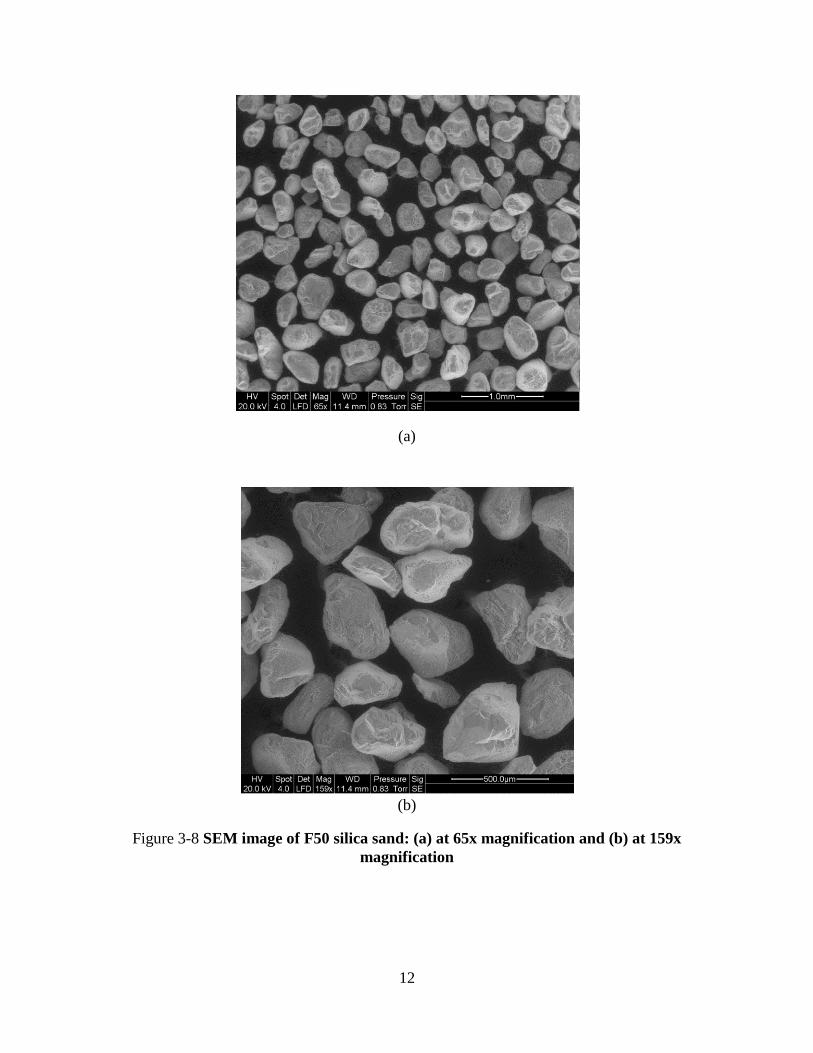
3.3.3 Scanning electron microscope (SEM)
To investigate the typical shape and the mineral composition of the F50 Ottawa sand, the
scanning electron microscope (SEM) and X-ray spectroscopy (EDS) tests were performed on this
sand. As Figure 3-8 shows SEM images proves that the sand particles are sub angular. As
expected, energy-dispersive X-ray spectroscopy (EDS) reveals that the dominant mineral
composition of the F50 Ottawa sand is quartz (Figure 3-9). It also showed that there are some
traces of aluminum oxides and other metal oxides in the mineral compositions as well.
12
(a)
(b)
Figure 3-8 SEM image of F50 silica sand: (a) at 65x magnification and (b) at 159x
magnification

13
Figure 3-9 Results from EDS spectrum for F50 Ottawa sand
3.3.4 Thermal conductivity
To determine the thermal conductivity of the sand and the concrete, two thermal conductivity
test setups were built during this study (Figure 3-10). These setups were similar to the ASTM
D5334 test which is for measuring thermal conductivity in soil and soft rock. The difference
between the apparatus used in this study and the ASTM test was that a heat carrying fluid was
used as the heat source instead of a heating probe. The diameter and height of the model equal
0.3m, and 0.6 m, respectively. Heat source was placed at the center of the mold. Same PVC tube
which was embedded within the model geothermal pile was used at the center of the thermal
conductivity test setup (outer diameter was 15.8 mm, and inner diameter was 12.4 mm).
Fourier’s law can be used to calculate thermal conductivity of the material inside the mold (soil
and concrete).

14
(a) (b)
Figure 3-10 Element test setup to measure thermal conductivity of sand and concrete: (a)
custom-built test apparatus and (b) temperature measurement locations
Fluid temperature at the inlet side was maintained at a constant value and the outlet fluid
temperature was monitored during the thermal conductivity tests. The system was allowed to
reach to the thermal equilibrium. Figure 3-11 shows the results for both concrete and soil thermal
conductivity tests and the equilibrium states. According to the Fourier’s law, based on the total
energy dissipated from the heat source to the media and radial soil temperature increments, the
thermal conductivity value k can be calculated. Equation (Error! Reference source not found.)
hows how the total energy can be predicted using the temperature difference between fluid inlet
and outlet points.
( )p in outE mC T T (3-2)
where E is the energy dissipated to the media, ṁ is the mass flow rate of the fluid which depends
on the circulation velocity and tube’s area, Cp is the specific heat capacity of the fluid, and Tin
and Tout are, respectively, fluid temperatures at the inlet and outlet points. While the system is in
the thermal equilibrium state (steady-state), Fourier’s law can be applied to determine thermal
conductivity of the material.
2p in out
1
1 2
( ) ln
2 ( )
rmC T T
rk
L T T
(3-3)
Tin
Tout
22.5 cm
7.5 cm
7.5 cm
22.5 cm
7.3
cm
7.3
cm
60
cm
30 cm
Outlet
Inlet
Insulation

15
where k is the material thermal conductivity, L is the length of the heat source, T1 and T2 are
temperature recorded at radial distances r1 and r2 from the centerline of the heat source
(circulation tube).

16
(a)
(b)
Figure 3-11 Thermal conductivity test results for (a) sand (b) concrete
0 20000 40000 60000 80000 100000
Time (s)
20
25
30
35
40
45
22.5
27.5
32.5
37.5
42.5
Te
mp
era
ture
T(°
C)
0
10
20
30
40
50
Po
we
r o
utp
ut
(W)
0 5 10 15 20 25Time (hour)
Power output
r1
r2
r3
He
at
circu
lation
tub
e
Data shown for circled
thermocouple locations
r1
r2
r3
a
Thermal conductivity test for soil, Tin= +40 °C
v=0.66 m/s
0 40000 80000 120000 160000 200000
Time (s)
20
25
30
35
40
45
22.5
27.5
32.5
37.5
42.5
Tem
pera
ture
T(°
C)
0
10
20
30
40
50
Pow
er
outp
ut (W
)
0 10 20 30 40 50Time (hour)
Thermal conductivity test for concrete, Tin= +40 °C
v=0.22 m/s
r1
r2
r3
Power outputa

17
3.3.5 Hydraulic conductivity
The hydraulic conductivity values for different void ratios (relative densities) for the F50 sand
were measured following ASTM D2434-68. As Figure 3-12 shows, hydraulic conductivity value
varies from 0.025 to 0.038 cm/s for the void ratio varying between 0.54 and 0.72.
Figure 3-12 Hydraulic conductivity of F50 Ottawa sand as a function of void ratio
Based on the sieve analysis, direct shear test, SEM, EDS and thermal conductivity tests, various
properties for the F50 Ottawa sand are summarized in Table 3-2.
Table 3-2 Properties of F50 Ottawa sand
Parameter Value Test Method
Shape Subangular Scanning Electron Microscope
Mineral composition > 99% Quartz Energy Dispersive Spectroscopy
Mean particle size, D50 (mm) 0.25 ASTM D6913
Coefficient of Uniformity, Cu 1.83 ASTM D6913
Coefficient of Curvature, Cc 0.95 ASTM D6913
Specific gravity, Gs 2.65 ASTM D854
Minimum void ratio, emin 0.48 ASTM D4253
Maximum void ratio, emax 0.78 ASTM D4254
Critical state friction angle, φc 31.8° ASTM D3080
Hydraulic conductivity (cm·s-1
) 0.025 to 0.038 ASTM D2434
Thermal conductivity, dry (W·m-1
·K-1
) 0.25 Cylindrical Heat Source
Thermal conductivity, moist (W·m-1
·K-1
) 2.65 Cylindrical Heat Source

18
3.4 Concrete model pile
To determine the various mechanical properties of the concrete pile, a series of cylinders were
cast along with the casting the model pile. These samples were cast in two ways (1) concrete
with an embedded U-shaped tube, (2) concrete only. Casting concrete samples with embedded
PVC tubing consider the loss of strength and stiffness compared to the homogenous mold. Table
3-3 presents the mechanical and thermal properties of the concrete used in thermal performance
tests. The embedded tubing resulted in a compressive strength reduction of 2.76 MPa (≈ 400 psi)
on average.
Table 3-3 Mechanical and thermal properties of concrete at 28 days
Compressive strength without tubing in MPa (psi) 44 (6,389)
Compressive strength with tubing in MPa (psi) 40.94 (5,939)
Elastic modulus in MPa (psi) 29730 (4,312,000)
Poisson’s ratio 0.11
Thermal conductivity (W/mK) 1.4
Specific Heat (J/Kg/C) 1000
Surface roughness of the pile was also measured along several representative sections of the
precast concrete in this study. Due to size restriction each section could not be more than 1 cm.
Pile-soil interface can be divided into two groups: perfectly smooth or perfectly rough (Basu et
al. 2011). Slip failure along the surface of the pile is the dominant failure for perfectly smooth
interface. Perfectly rough interface creates shear bands near the vicinity of the pile interface.
Normalized roughness Rn which represents the pile interface condition is calculated by dividing
the maximum roughness of the pile surface Rmax by the mean particle size of the soil (D50). Rmax
obtained from optical profilometry equal to 20 μm (Figure 3-13). As mentioned earlier D50 of for
the F50 Ottawa sand used in this study is 0.25 mm. Therefore, Rn value equal to 0.08. Based on
the Rn value the pile-soil interface can be considered as a perfectly rough interface (Uesugi and
Kishida 1986, Uesugi et al. 1988, Lings and Dietz 2005, Basu et al. 2011). Therefore, critical
state friction angle (31.8°) can be considered as an interface friction angle for perfectly rough
pile-soil interface.

19
Figure 3-13 Surface roughness profile for the concrete model pile
3.5 Instrumentation and data acquisition
3.5.1 Thermocouples
To investigate the thermal performance of the geothermal pile, soil temperature was monitored at
94 locations inside the sand deposit as well as at the inlet and outlet fluid points. Type T
thermocouples which can measure temperature range of −200°C to 350°C with an accuracy of ±
0.5 °C were selected in this research. Type T thermocouples have a pair of twisted wires: one
copper and the other constantan (copper-nickel alloy). Thermocouples has two ends, hot ends
which is basically a twisted of two different wires and cold ends which is left unpaired. The cold
end should be connected to the data acquisition (DAQ) system. As mentioned earlier temperature
increments was monitored at 94 locations within the sand bed, on pile surface, tank boundaries
and within the circulation tube. Figure 3-14(a) shows the layout of the thermocouples locations
on a plane passing through the pile and the circulation tube (hereafter referred to as XZ plane).
With the selected layout, we could monitor the warm side and cold side of the pile. Between
these two extreme sets of temperature records (warm side and cold side), temperature was also
measured at different points on the YZ plane. Figure 3-14(b) also shows the layout of
thermocouples locations on a plane perpendicular to the plane containing the circulation tube
(hereafter referred to as YZ plane).
From 94 thermocouples 17 locations were selected along the pile surface, eight thermocouples at
each side and one at the pile base. Six thermocouples were placed at the tank boundary and
another six thermocouples were placed at the top of the sand bed. The rest of 94 thermocouples
were placed within the sand bed. Besides than these 94 locations, temperature was also recorded
at the fluid inlet and outlet points. Having temperature readings at the inlet and outlet points is
necessary to quantify the heat exchange efficiency of the system. All of the 96 thermocouples
were connected to a total of six NI 9213 modules. Each of these modules is capable to acquire 16

20
differential voltage inputs at an aggregate data acquisition rate of 75 samples per second per
channel (S/s/ch). All the modules were connected to the NI cDAQ 9178 chassis. Temperature
measurements were collected, displayed, and logged in real time at a rate of 0.1 Hz using data
collection software written in LabVIEW 2011 (National Instruments 2013) (Kramer 2013,
Kramer and Basu 2014a, 2014b, Kramer et al. 2014).
(a) (b)
Figure 3-14 Temperature measurement locations: (a) XZ plane and (b) YZ plane
3.5.2 Load cell and displacement sensor
Omega LCM401-2.5K load cell was placed between the pile helmet and load cylinder to control
the amount of mechanical loading applied by a hydraulic jack (Enerpac RC-55). The load cell
was connected to an NI 9205 module housed in the same NI cDAQ 9178 chasis which housed
the thermocouples modules. The load cell module has an aggregate sampling rate of 250×103
S/s. The data was gathered, logged, and displayed in real time at an acquisition rate of 2 Hz using
the Labview code (Kramer 2013, Kramer and Basu 2014a, 2014b, Kramer et al. 2014).
Two linear variable differential transformers (LVDTs) were used to monitor top and bottom
displacements of the pile. Both LVDTs used in this research were Omega LD621-100. The
LVTD can measure the displacement up to 10.6 cm. Both LVDTs were connected to the NI 9205
which was previously housed for the load cell. One of the LVDTs, that was used to measure the
pile head displacement, was fixed to the load cylinder and its tip was exactly placed on the pile
helmet. A telltale rod was used to measure the pile base displacement. The other LVDT was
attached to the telltale to monitor the displacement of the telltale. The telltale was composed of a
0.3175 cm steel rod that lies inside a plastic tube. The plastic tube was used to separate steel rod
from the concrete. The displacement of the rod is independent of the pile compression and it only
410
(in)16 10 6
(cm)
(cm)40.6 25.4 15.2
(in)
8
12
9
3
12
12
12
1.1
7 m
(4
6 in
)
y
20.3
30.5
22.9
7.6
30.5
30.5
30.5
z(in)16 10 6 6 10 16(cm)40.6 25.4 15.2 15.2 25.4 40.6
2 @ 42@10
(in)
8
12
9
3
12
12
12
1.1
7 m
(4
6 in
)
z
x
20.3
30.5
22.9
7.6
30.5
30.5
30.5

21
shows the pile base settlement. However, the LVDT at the top of the pile measured both pile
settlement and pile compression.
3.5.3 Labview code
Data logging software was developed in Labview using a graphical interface (GUI) to present the
results in real time (Kramer and Basu 2014a, 2014b, Kramer et al. 2014). The program
developed in Labview is capable to acquire and process the data in parallel. Aggregate
acquisition rates can be as fast as 75 samples per second per channel (S/s/ch). However,
considering a couple of days for a time scale of the thermal performance tests, samples were
acquired at a rate of 2 S/min/ch. Figure 3-15 shows a temperature contour which was presented
by Labview code at both XZ and YZ planes. Linear approximation was used to estimate the
temperature for the nodes between the thermocouple locations.
Figure 3-15 Temperature contours displayed by the developed labview code
Model pile displacements and the axial load were also collected and displayed on the same GUI.
The GUI shows three graphs, (1) axial load versus a real time, (2) pile head and pile base
displacement versus time, (3) pile head displacements versus the axial load. Figure 3-16 shows
these three graphs in a single screen shot.

22
Figure 3-16 Axial load and pile head and base displacements displayed by the developed
labview code
For data acquisition aggregate sampling was used to reduce the noise. The rate used to acquire
that load-displacement data was 1 S/s/ch. However a given data was actually the average of 100
measurements made at a rate of 1000Hz. Since, very high data acquisition rates were required; a
producer-consumer architecture was used to separate data acquisition from display and logging
(Kramer 2013, Kramer et al. 2013). The developed GUI code has two major benefits, (1) the
load versus time graph would confirm that the loading steps were consistent, (2) the load
displacement curve shows the start of plunging behavior that could be used as an indicator to
terminate a load test.
3.6 Results
3.6.1 Thermal performance
Inlet fluid temperature was kept constant during each thermal loading test using a temperature-
controlled water bath. Heat carrier fluid was circulated from the constant temperature water bath
to the tubing embedded within the model geothermal pile. As mentioned in previous section,
temperature increments were measured at 94 locations within the soil and along the pile. The
thermal conductivity and specific heat capacity of the sand, and the concrete pile, are assumed to
be constant for all tests under dry condition. Same assumption is valid for the saturated
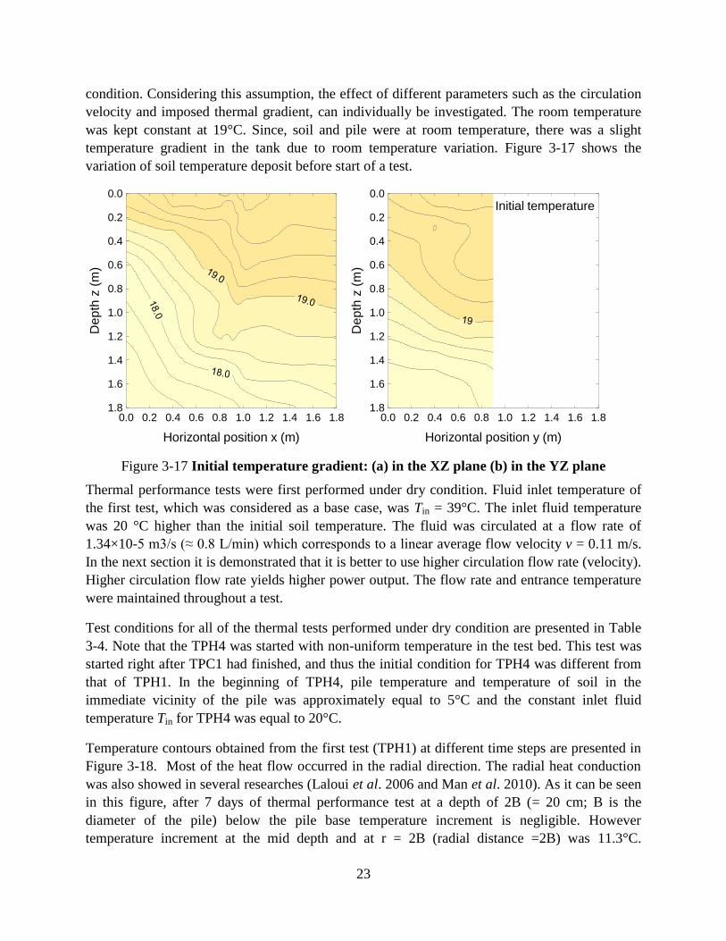
23
condition. Considering this assumption, the effect of different parameters such as the circulation
velocity and imposed thermal gradient, can individually be investigated. The room temperature
was kept constant at 19°C. Since, soil and pile were at room temperature, there was a slight
temperature gradient in the tank due to room temperature variation. Figure 3-17 shows the
variation of soil temperature deposit before start of a test.
Figure 3-17 Initial temperature gradient: (a) in the XZ plane (b) in the YZ plane
Thermal performance tests were first performed under dry condition. Fluid inlet temperature of
the first test, which was considered as a base case, was Tin = 39°C. The inlet fluid temperature
was 20 °C higher than the initial soil temperature. The fluid was circulated at a flow rate of
1.34×10⁻⁵ m3/s (≈ 0.8 L/min) which corresponds to a linear average flow velocity v = 0.11 m/s.
In the next section it is demonstrated that it is better to use higher circulation flow rate (velocity).
Higher circulation flow rate yields higher power output. The flow rate and entrance temperature
were maintained throughout a test.
Test conditions for all of the thermal tests performed under dry condition are presented in Table
3-4. Note that the TPH4 was started with non-uniform temperature in the test bed. This test was
started right after TPC1 had finished, and thus the initial condition for TPH4 was different from
that of TPH1. In the beginning of TPH4, pile temperature and temperature of soil in the
immediate vicinity of the pile was approximately equal to 5°C and the constant inlet fluid
temperature Tin for TPH4 was equal to 20°C.
Temperature contours obtained from the first test (TPH1) at different time steps are presented in
Figure 3-18. Most of the heat flow occurred in the radial direction. The radial heat conduction
was also showed in several researches (Laloui et al. 2006 and Man et al. 2010). As it can be seen
in this figure, after 7 days of thermal performance test at a depth of 2B (= 20 cm; B is the
diameter of the pile) below the pile base temperature increment is negligible. However
temperature increment at the mid depth and at r = 2B (radial distance =2B) was 11.3°C.
0.0 0.2 0.4 0.6 0.8 1.0 1.2 1.4 1.6 1.8
Horizontal position x (m)
1.8
1.6
1.4
1.2
1.0
0.8
0.6
0.4
0.2
0.0
De
pth
z (
m)
0.0 0.2 0.4 0.6 0.8 1.0 1.2 1.4 1.6 1.8
Horizontal position y (m)
1.8
1.6
1.4
1.2
1.0
0.8
0.6
0.4
0.2
0.0
De
pth
z (
m)
Initial temperature

24
Significant heat loss was also observed at the ground surface of the sand deposit. Thus, we can
conclude that there is a significant convective heat transfer from the soil surface.
Table 3-4 Thermal performance test matrix
Test name Heating vs cooling Initial temperature
gradient °C
Circulation velocity v
(m/s)
TPH1 Heating +20 0.11
TPH2 Heating +20 0.33
TPH3 Heating +20 0.66
TPH4 Heating +15 0.11
TPC1 Cooling −20 0.11
TPC2 Cooling −20 0.66
TPSCH Cooling followed by
heating −20 and +35 0.66
Figure 3-18 (a)
z
x
y
Thermocouples
were placed on
the hatched planes
(XZ and YZ)

25
Figure 3-18 (b)
Figure 3-18 (c)
z
x
y
Thermocouples
were placed on
the hatched planes
(XZ and YZ)
z
x
y
Thermocouples
were placed on
the hatched planes
(XZ and YZ)

26
Figure 3-18 (d)
Figure 3-18 (e)
Figure 3-18 Temperature evolutions (contours) at different time steps
Thermal influence zone was also identified in this research. It will be showed later in the
numerical model section that the soil temperature beyond the thermal influence zone would not
be changed even after 2 months of operation. Soil temperature increments along the depth at r =
2B at different time steps are presented in Figure 3-19. As it can be seen in this figure,
temperature at r = 10 cm increases by 9 °C in 2 days and in the following 5 days (at t=7 days) it
only increases by 2 °C. This shows a drastic change near the geothermal pile within a short time
z
x
y
Thermocouples
were placed on
the hatched planes
(XZ and YZ)
z
x
y
Thermocouples
were placed on
the hatched planes
(XZ and YZ)

27
after the start of the test and the temperature reaches to a somehow steady state condition in a
couple of days.
Figure 3-19 Soil temperature Tg measured at different thermocouple locations at r = 2B
As heat dissipated from the heat source into the surrounding soil, a zone of thermal influence
was evident within the soil. Soil temperature will not significantly change (less than a degree)
beyond this zone. Temperature evolutions ΔTg (under dry condition) at different radial distances
with both real and normalized time (expressed as Fourier number Fo) for two different tests (one
heating and one cooling) are presented in Figure 3-20. At radial distances farther from the pile
the amount of time to experience a change in temperature is higher. Soil temperature at r=0.5B
(= 5 cm) away from the pile increases in only 15 minutes after the heat transfer started. Whereas,
for the same test, same amount of temperature increments for a point at a distance of 10B (= 50
cm) away from the pile take 24 hours. Moreover, it could be confirmed that (as expected), with
all other parameters identical heating (Δθ = 20°C) and cooling (Δθ = −20°C) produce identical
but opposite thermal responses in soil.

28
Figure 3-20 Temperature evolution with normalized and real time
During the seven days of thermal performance test, only the zone near the geothermal pile
reached to a nearly steady state condition. However, the pile-soil system was still in a transient
heat flow condition. By the end of seven days, soil temperature at the tank boundary did not
change, so there was not any heat loss from the tank boundaries during the test duration. In real
condition there is not any side boundary and, therefore, heat would not dissipate to the outside of
the media, except possibly from the surface. Therefore, all the thermal performance tests were
stopped while heat reached to the tank boundary. Figure 3-21 also shows that the inlet side of the
pile was slightly warmer than the outlet side of the pile at all measurement points.
0.01 0.1 1 10 100
Normalized time Fo
-20
-10
0
10
20
So
il te
mp
era
ture
incre
me
nt
Ts (
°C)
TPH1, = + 20 °C v=0.11 m/s
TPC1, = – 20 °C v=0.11 m/s
0.01 0.1 1 10Time t (days)
r=0.05 m
r=0.10 m
r=0.25 m
r=0.50 m
r = 0.05 m r = 0.10 m r = 0.25 m r = 0.50 m

29
Figure 3-21 Radial distribution of Soil temperature evolution
Fluid temperatures at the inlet and outlet points of the circulation tube were recorded during the
test. The amount of power output can be calculated from the temperature difference ΔTf between
these two points. Circulation flow rate is one the key parameters which can change the power
output of the system. To study the effect of circulation flow rate (or circulation velocity) on the
efficiency of the model geothermal pile, three different circulation flow rate (three different
thermal load tests) were considered under dry condition. The circulation velocities of these tests
were respectively, 0.11 m/s (the base case), 0.33 m/s and 0.66 m/s.
The energy output E over a certain period of heat transfer through the model geothermal pile can
be viewed as a representation of thermal power output P (energy extraction/rejection rate) (or
heat transfer efficiency) of the pile. Mathematically,
pf f f pf in out P mC T vAC T T (3-4)
where ṁ is the mass flow rate of the circulation fluid, CPf is the specific heat capacity of the
circulation fluid, and ΔTf is the fluid temperature difference between the inlet and outlet points.
The mass flow rate ṁ can be determined by multiplying volumetric flow rate by the density of
the circulation fluid. As Figure 3-22 shows an increase in the flow rate of the circulation fluid
increases the power output.

30
Figure 3-22 Geothermal power output obtained from a mode pile for different circulation
flow rate
There are both daily short-term variations as well as long-term seasonal variations in air
temperature. Therefore, cyclic thermal loads should be investigated to predict power output
obtained from the real geothermal pile. Soil surrounding these piles would be subjected to heat
extraction during winter followed by heat rejection during summer months (or heat extraction
during the night followed by heat rejection during the day). To investigate the effect of thermal
cycle loading on heat transfer performance of the geothermal model pile, a cyclic load test (test
TPSCH) was performed. Deicing the bridge decks starts in winter and the system can be
continuously working to reject heat into the ground and recharge it in future. To model the real
thermal loading cycles, heat was first extracted from the soil (Δθ = −20°C, Tin = 0 °C) for seven
days and then immediately heat extraction phase was started. Results obtained from the cyclic
test showed that thermal efficiency of the system for a short duration in the initial part of the
second phase of thermal loading was increased by 30% compared to that obtained from the first
half of thermal loading with Δθ = −20°C (Figure 3-23). This occurred due to the presence of high
thermal gradient (Δθ = 35°C) at the onset of thermal loading reversal and the availability of
additional thermal storage in the soil immediately after the heat extraction phase. However, by
depleting the initial thermal potential, the system approached similar steady state efficiency for
both phases of thermal loading. Real life situation may also include some intermediate thermal
loading phases (or even no operation at all) during intermediate seasons (e.g., late spring and
early fall) in between the extreme thermal loadings during winter and summer or during the day
and night. Such intermediate phases of operation (or temporary pause in thermal operational)
affect heat transfer efficiency of the system for a short period of the time. Numerical simulation
also showed the same trend.
0 10 20 30 40
Normalized time Fo
0
20
40
60
80
100
120
Pow
er
ou
tput
pe
r un
it leng
th o
f th
e p
ile P
/Lp (
W/m
)
TPH1, = + 20 °C, v=0.11 m/s
TPH2, = + 20 °C, v=0.33 m/s
TPH3, = + 20 °C, v=0.66 m/s
0 2 4 6Time t (days)

31
Figure 3-23 Effect of sequential heat extraction and rejection on geothermal power output
Mechanical load tests were performed on the model pile before and after the heat exchange
operation. Free displacement condition was maintained at the pile head and pile head and base
displacements were measured continuously during the load tests. A load increment of 0.1 kN was
used for all tests. Figure 3-24 shows a small increase in limit load after the thermal load was
applied for seven days. The initial pile head stiffness decreases after the thermal loading.
0 5 10 15 20 25 30 35 40
Normalized time Fo
0
20
40
60
80
100
120
140
Po
we
r o
utp
ut
pe
r u
nit le
ng
th o
f th
e
pile
P/L
p (
W/m
)0 2 4 6
Time t (days)
0 5 10 15 20 25
Normalized time Fo
0 2 4Time t (days)
Heat extraction phase of TPSCH
= – 20 °C, v=0.66 m/s
Heat injection phase of TPSCH
= + 35 °C, v=0.66 m/s

32
Figure 3-24 Axial load-displacement behavior of the model geothermal pile before and after
thermal loading
3.7 Observations from thermal tests
A number of observations were made based on the data recorded during a series of thermal load
tests on the model geothermal pile. It was observed that heat flow through geothermal piles
occurs primarily in the radial direction. The heat dissipation raises the temperature of the soil in
the vicinity of the pile within a ‘thermal influence zone’ that expands with time. When designing
geothermal piles, particularly if they are to be installed as part of a pile group, the thermal
efficiency of these piles will reduce if the zones of thermal influence overlap with one another.
Results show that increasing the flow rate of the heat carrier fluid will increase the energy output
of the pile. The geothermal piles have high initial energy outputs that approach steady-state
values as the soil surrounding the pile begins to change temperature. The steady-state energy
output values should be used for design because such values represent long-term thermal
behavior. However, running heating and cooling cycles in series does provide an increased short-
term efficiency.
The model geothermal pile was subjected to a series of mechanical load tests at ambient
conditions as well as during thermal loading. During all mechanical load tests, plunging of the
pile, that signifies typical limit state behavior, was observed. Based on interpretation of the pile
load tests performed, it appears that both limit- and ultimate-state capacities of geothermal piles
are likely to be affected by thermal loading.
0 1 2 3 4
Axial load (kN)
2.50
2.00
1.50
1.00
0.50
0.00
Hea
d d
isp
lace
men
t (m
m)
Free head condition
Mechanical loading at initial temperature (20°C)
Mechanical loading at elevated temperature (40°C)

33
4. Laboratory-scale tests on bridge deck (concrete slabs)
To test the viability of a ground-source bridge deck deicing system, a field test setup was
constructed at the Virginia Tech Geotechnical Research Facility. The setup consisted of a small-
scale bridge deck connected to geothermal piles installed in the field. There were several
purposes of the field test. The first of which is to provide proof of concept testing to demonstrate
that ground-source bridge deck deicing is a viable concept. The second reason was to provide
data for numerical model calibration.
4.1 Field test setup and construction
The field test setup consists of a total of five micropiles, four of which are equipped with
circulation loops along the full pile length for heat exchange. Test piles, 25-cm (10 inches) in
diameter, were installed to a depth of approximately 30.5 meters (100 feet) as part of a previous
research project (Abdelaziz 2013). The energy piles are instrumented to measure strains and
temperatures at about every 3m (10ft). The piles are embedded in a silty sand, which extends to a
depth of 12.2m (42ft), after which is a weak shale layer. There are also four observation
boreholes installed around the piles that can measure temperatures in the ground. The plan view
of the pile and borehole locations is shown in Figure 4-1. Table 4-1 provides the depths at which
temperature and strain (if applicable) were recorded in each of the boreholes and piles.
Pile 4 Pile 3
Pile 1 Pile 2Reaction
Pile
2.50m. 2.90m.
1.20m.
2.50m. 2.50m.
0.45m.
0.45m.
2.5
0m
.
2.5
0m
.
0.9
0m
.
0.9
0m
.
1.2
0m
.
Observation Point #4
Observation Point #1
Observation Point #3
Observation Point #2
Figure 4-1 Plan view of the energy pile and borehole locations

34
Table 4-1 Locations of recorded measurements in the energy piles and ground
Location Depths Measured (m)
Piles 2 and 3 (Temperature and
Strain)
3.0, 6.1, 9.1, 12.2, 15.2, 18.2, 21.3, 24.3, 27.4, 30.4
Observation Points 1 and 2 3.0, 6.1, 9.1, 12.2, 15.2, 18.2, 22.8, 27.4, 30.4
Observation Point 3 3.0, 6.1, 10.6, 15.2
Observation Point 4 3.0, 6.1, 9.1, 12.2, 15.2, 18.2, 21.3, 24.3, 27.4, 30.4, 33.5,
36.5
A prototype 2.4 m x 3.0 m (8 ft. x 10 ft.) bridge deck was constructed as shown in Figure 4-2.
The doubly reinforced 25 cm (10 inch) thick slab is elevated from the ground to simulate heat
loss from the bottom face similar to a bridge deck. The test slab is divided into two 1.2 m x 3.0 m
(4 ft. x 10 ft.) sections with an insulated separation in between. A 5 cm (2 inch) thick clear
concrete cover is present on top of the upper level reinforcement. PEX tubes with 16 mm (5/8
inch) inner diameter (ID) are connected to the upper level reinforcement with 20 cm (8 inch) and
30 cm (12 inch) horizontal spacing in each section. Insulation has been added to the sides to
simulate an adiabatic surface. The slab is heavily instrumented with 36 thermistors to monitor
the variation of temperature in both slab sections at different horizontal and vertical extents near
the tubes.
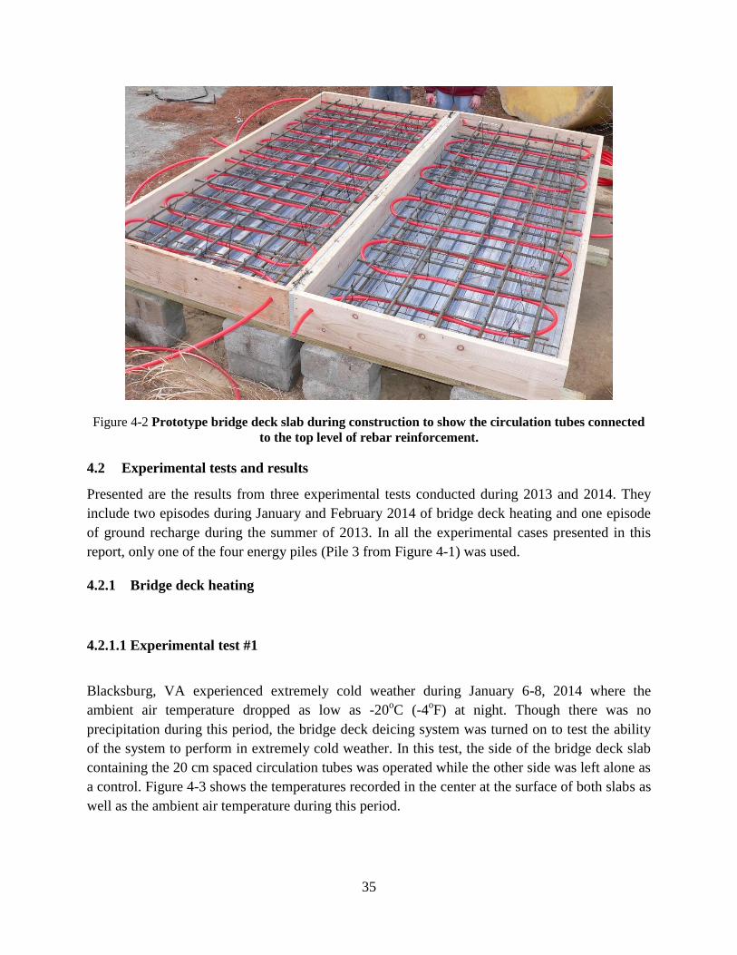
35
Figure 4-2 Prototype bridge deck slab during construction to show the circulation tubes connected
to the top level of rebar reinforcement.
4.2 Experimental tests and results
Presented are the results from three experimental tests conducted during 2013 and 2014. They
include two episodes during January and February 2014 of bridge deck heating and one episode
of ground recharge during the summer of 2013. In all the experimental cases presented in this
report, only one of the four energy piles (Pile 3 from Figure 4-1) was used.
4.2.1 Bridge deck heating
4.2.1.1 Experimental test #1
Blacksburg, VA experienced extremely cold weather during January 6-8, 2014 where the
ambient air temperature dropped as low as -20oC (-4
oF) at night. Though there was no
precipitation during this period, the bridge deck deicing system was turned on to test the ability
of the system to perform in extremely cold weather. In this test, the side of the bridge deck slab
containing the 20 cm spaced circulation tubes was operated while the other side was left alone as
a control. Figure 4-3 shows the temperatures recorded in the center at the surface of both slabs as
well as the ambient air temperature during this period.

36
Figure 4-3 Surface temperatures of the heated and unheated bridge deck slabs during bridge deck
heating.
From Figure 4-3, several observations can be made. The first is that the bridge deck deicing
system was able to significantly heat the slab, causing the surface temperature of the heated slab
to be as much as 15oC (27
oF) higher than the unheated slab. However, despite the significant
difference between the performances of the two slabs, the system was not able to keep the
surface temperature of the heated slab above 0oC (32
oF) meaning that if any precipitation were to
accompany this extreme cold weather event, it would accumulate on the surface of the deck. It
should be noted, however, that these extreme environmental conditions are well outside the
range of those expected during normal operation.
4.2.1.2 Experimental test #2
Another test of the deicing system occurred on January 21, 2014. Beginning around 11AM and
continuing until 4PM, approximately 2.0 cm (0.8 in) of snowfall occurred. The system was
turned on in advance of the storm at 7AM. Figure 4-4shows the ambient air temperature, the
temperatures of the surface of both the heated and unheated decks, as well as the cumulative
amount of precipitation that fell. Note that the system was turned on when temperatures of both
the heated and unheated surfaces of the deck were decreasing. After the beginning of operation,
the heated deck surface temperature increased to approximately 4oC (39
oF) by the time the snow
started to fall and maintained a temperature above 4oC for the duration of the event. The
-25
-20
-15
-10
-5
0
5
10
15
6 7 8 9 10
Te
mp
era
ture
, oC
Day of January 2014
Heated - Above Tube
Heated - Between Tubes
Non-Heated
Air Temperature
Operation

37
unheated deck maintained a temperature around 0oC (32
oF). The system was able to keep the
deck completely snow free for the entire duration of the test, whereas snow accumulated on both
the unheated side and the control slab (Figure 4-5).
Figure 4-4 Ambient air temperature, precipitation, and temperature at the surface of the heated
and unheated decks during bridge deck deicing.
Figure 4-5 Photographs comparing performance of the heated deck vs. unheated deck (left) and the
control slab (right).
4.2.1.3 Experimental test #3
The capabilities of this system were tested again during a winter storm that occurred on February
21, 2015. This winter storm consisted of 16.5cm (6.5in) of snow that began falling while the
0
0.4
0.8
1.2
1.6
2
2.4
2.8
-10
-8
-6
-4
-2
0
2
4
6
8
10
0:00 3:00 6:00 9:00 12:00 15:00 18:00 21:00 0:00
Cum
ula
tive
Am
ou
nt o
f S
no
w,
cm
Te
mp
era
ture
, oC
Time of Day on 1/21/2014
Heated - Above Tube
Heated - Between Tubes
Non-Heated
Ambient Air
Snowfall
Operation Begins

38
ambient air temperature was -13oC (8
oF). Furthermore, these extremely cold temperatures
(atypical for Blacksburg, VA) had persisted for several days, becoming as low as -20oC (-4
oF).
Thus, the slab was -18oC when the system was turned on the day before in anticipation of the
storm. Again, only one half of the slab was operated. The surface temperatures of the heated
slab, non-heated slab, and the ambient air temperature are shown in Figure 4-6.
Figure 4-6 Ambient air temperature and surface temperatures of the heated and nonheated slabs
From this test, several observations can be made. The first of which is that using only the thermal
energy from the ground as extracted from one energy pile, the system was able to heat the 20cm
side of the bridge deck over 18oC before the start of the storm. This both exemplifies the
capabilities of these systems and demonstrates how important it is to preemptively turn these
systems on in anticipation of a storm so that they can adequately heat the deck. The second
observation is that the surface temperatures of the heated deck were heated to values greater than
0oC. Though this system was not able to keep the deck completely free from snow, it was able to
maintain a surface temperature greater than 0oC indicating that when combined with mechanical
removal (which will be required anyway for 16.5cm of snow), a snow-free deck surface will
result.
4.2.2 Ground response to bridge deck heating
Figure 4-7 displays the temperatures along the pile at different points during operation of the
system during the experimental test presented in section 4.2.1.1. Though temperature was
measured at 3m intervals, not all are shown to reduce clutter in the graphs. Rather, two locations
from each soil layer (the silty sand and the shale) are plotted to develop the temperature profile
vs depth.
-20
-15
-10
-5
0
5
10
15
2/20 2/21 2/22 2/23
Tem
per
atu
re, o
C
Date
Heated - Above Tubes
Heated - Between Tubes
Nonheated
Air Temperature
Operation Begins
Snowfall Period

39
Figure 4-7 Temperatures along the pile at different times during operations
In Figure 4-7, one can observe that the starting temperatures are not the same for each depth
indicating a non-uniform temperature distribution with depth in the ground. In fact, the 9.1 m
depth is the highest of all observed temperatures and the 3.0 m depth is the lowest. This is
expected as explained in Kusuda and Achenbach (1965). The depths closer to the surface will
experience greater temperature variation as the mean ambient air temperature fluctuates
throughout the year. As one moves deeper in the soil profile, the amplitude of temperature
variations are not as great and are somewhat ‘lagging’ with respect to the temperatures in the soil
above.
One can also observe that temperatures in the pile decrease after operation of the system begins,
with the 30.4m depth exhibiting an almost 5oC temperature decrease. Temperatures continue to
decrease from 12 to 24 hours of operation, but here a distinction can be made. The two depths in
the silty sand (3.0m and 9.1m) do not experience much, if any, temperature change after 24 hours
whereas the depths in the shale (15.2m and 30.4m) experience temperature fluctuations after 24
hours. More will be explained later regarding this. For all depths except the 9.1m, the lowest
temperatures in the pile occurred at 24 hours.
Figure 4-8 records the temperatures along the pile after the system operation has ended, thus
characterizing the recovery period. For reference, it includes the initial temperature profile along
the pile before operation began. The temperatures recover very quickly in the first 24 hours, with
every location except the 3.0m depth recovering at least half of their temperature loss at the end
of operation. The 30.4m and 15.2m depths recover the fastest and after 120 hours all depths
except the 3.0m have been restored to their initial values.
0
5
10
15
20
25
30
35
0 2 4 6 8 10 12 14
Dep
th, m
Temperature, oC
Initial
12
24
36
53 (End)

40
Figure 4-8 Temperature vs depth along the pile for different instances in time after operation ended.
To better understand how the temperatures in the pile and ground change over time, the
temperature change in the locations mentioned previously were plotted vs time and are shown in
Figure 4-9. The ground temperatures were recorded in Observation Well 1, which is a distance of
1.7 m (5.7 ft) away from Pile 3.
Figure 4-9 Temperatures in the pile (top) and ground (bottom) as recorded at Observation Point 1
After operation begins, the temperatures in the pile immediately decrease, as can be seen in
Figure 4-9. This decrease, however, is not uniform with depth as seen in Figure 4-7. The 30.4 m
depth experiences the greatest decrease in temperature, followed by the 15.2 m depth, the 3.0 m
depth, and the 9.1 m depth. There are a couple of possible explanations. The first is that several
of the sensors may be closer to the circulation tubes than the other. If the location of the sensors
was the only factor, one would expect that once the pile reaches steady-state (roughly the period
of time between day 7.5 and 8.5), the temperatures would be about the same value, and they are
0
5
10
15
20
25
30
35
0 2 4 6 8 10 12 14
Dep
th, m
Temperature, oC
Initial
End (Time 0)
12
24
48
72
120
-10
-8
-6
-4
-2
0
3.0m Depth 9.1m Depth
15.2m Depth 30.4m Depth
-1
-0.75
-0.5
-0.25
0
6 7 8 9 10 11 12 13 14 15
Day of January 2014
Te
mpe
ratu
re C
ha
ng
e,
oC
Operation

41
not (Loveridge and Powrie 2014). Furthermore, after the system is turned off around day 8.5, the
recovery curves (the portion of the curves that occur after day 8.5 when the system is recovering)
are different.
To explain this, consider the site stratigraphy. The top 12 m (40 ft) of the site is a silty sand.
Underlying the silty sand is a shale and the water table is located at this boundary. When giving
design recommendations on geothermal systems, ASHRAE (2011) states that the thermal
conductivity of light sand with 5% water is 1.0 to 2.1 W/mK (0.5 to 1.1 Btu/h-ft-oF) whereas the
thermal conductivity of wet shale is 1.4 to 2.4 W/mK (0.8 to 1.4 Btu/h-ft-oF) meaning heat
transfer can occur more easily in the shale layer than in the silty sand. Thus, more energy would
be drawn from the shale layer than the silty sand resulting in lower temperatures in the shale
layer. The top plot in Figure 4-9 shows that this is the case with both the 30.4 m and 15.2 m
depth curves showing lower temperatures than the curves from the depths in the silty sand.
Further evidence of this is the fact that the recovery curves for the lower two depths show a
faster recovery than those for the higher depths, meaning that heat is flowing more quickly into
those parts of the system, possibly due to the higher thermal conductivity. Another factor for the
shape of these curves is the boundary conditions at either end of the pile. The ground at the top
of the pile is subjected to atmospheric conditions (which are very cold as can be seen in Figure
4-3), whereas the ground below the pile is a more or less constant temperature of 13oC (55.4
oF).
Thus, the higher temperature at the lower boundary and the higher thermal conductivity in the
lower layer combine to produce a sharper (or quicker) recovery curve.
Also notice the slopes of the temperature curves in the bottom plot of Figure 4-9 and how they
vary with time. It should be noted that some variation with time is expected as the temperatures
fluctuate in the ground naturally at the 3.0m depth. At the end of the observation period (day 15),
the temperatures in the ground for the 3.0 and 9.1 m depths are still decreasing whereas the
temperatures in the ground for the 15.2 and 30.4 m depths have either stopped decreasing (15.2
m) or begun to increase again (30.4 m). Operation of the system creates a negative temperature
gradient around the pile, which drives heat flow towards the pile. A higher thermal conductivity
would allow the temperature gradients around the pile to stabilize more quickly, as evidenced by
this plot.
4.3 Ground Thermal Recharge
While the previous experimental tests focused on bridge deck heating, experimental tests were
also conducted for ground recharge – to see if the temperature in the ground could be increased
and, in effect, store heat in the ground for use in the winter. A series of recharge operations were
performed over several warm days in June of 2013. Figure 4-10 contains the plots of the
temperatures in the pile and in the ground for depths of 3.0, 9.1, 15.2, and 30.4 m. Note that in
the top of Figure 4-10, each spike in the temperature curve corresponds to a recharge operation.
Several observations can be made. The first is that during heat injection, the temperatures near
the bottom of the pile increase more than the temperatures at the top, just as they decreased more

42
during bridge heating. Furthermore, the recovery curves at the end of each heating cycle are
steeper for both of the lower depths, which are located in the shale. This again indicates a higher
thermal conductivity for the shale layer.
Figure 4-10 Temperatures in the pile (top) and ground (bottom – measured in observation well 1)
during ground thermal recharge.
Observe the relative increase in the temperatures of the ground at each depth (bottom of Figure
4-10). At the end of the observation period (July 10), the temperatures in the ground for the 3.0
and 9.1 m depths are still increasing whereas the temperatures in the ground for the 15.2 and 30.4
m depths have either stopped increasing (15.2 m) or begun to decrease (30.4 m). During recharge
operations, the system creates a positive temperature gradient around the pile, which drives heat
flow outwards from the pile. Similar to bridge deck heating, the higher thermal conductivity of
the shale layer results in quicker temperature stabilization at the lower depths.
The question still remains as to whether any heat was successfully stored in the ground for use in
the winter. To answer this question, some idea of what the temperatures in the ground should be
with no heating is needed. Observation well 2 is located 3.5 m (10.7 ft) from the test pile.
Although the effects from heating could still affect the temperature of the ground at this distance,
the effect will be less pronounced than at the energy pile and at observation well 1, which is only
1.7 m from the pile. Thus, the observation well further away can serve as a control. The net
temperature difference between observation well 1 (which is representative of the ground), the
energy pile, and the observation well 3.5 m from the energy pile is shown in Figure 4-11.
11
13
15
17
19
21
10
11
12
13
14
10-Jun 15-Jun 20-Jun 25-Jun 30-Jun 5-Jul 10-Jul
Date
3.0m Depth 9.1m Depth 15.2m Depth 30.4m Depth
Te
mpe
ratu
re,
oC

43
Figure 4-11 Net temperature difference in the ground over time after ground thermal recharge between
OW-A (top) and the energy pile (bottom) relative to OW-B.
From Figure 4-11, it is clear that at every depth there was a positive temperature increase in the
ground at OW-A relative to OW-B, and in the pile relative to OW-B. The largest increase in
temperature occurs at the top two depths, which is where the soil with the lower thermal
conductivity is located. The highest sustained temperature increase appears to be in the middle
two depths (9.1 m and 15.2 m). This is most likely due to the fact that the 3.0 m and 30.4 m
depths experience heat loss through the ground surface and to the ground below, respectively.
0
0.2
0.4
0.6
0.8
1
1.2N
et
Tem
pera
ture
D
iffe
rence,
oC
0
0.2
0.4
0.6
0.8
1
1.2
0 20 40 60 80 100 120 140 160 180 200
Net
Tem
pera
ture
D
iffe
rence,
oC
Days from May 10, beginning of summer
3.0m Depth
9.1m Depth
15.2m Depth
30.4m Depth
Ne
t T
em
pe
ratu
re D
iffe
ren
ce,
oC

44
Table 4-2 summarizes the measured difference in temperature for the pile and ground relative to
the temperature difference of the ground at a distance of 3.5 m from the pile during this period of
time. For every depth except the 3.0 m depth for the ground 1.7 m from the pile, there was a
positive temperature difference between it and the ground 3.5 m from the pile. The same is true
for the pile. Thus, it does appear that heat was successfully stored in the ground; however, the
relative temperature differences are very small. The small temperature difference may be due to
the fact that there were only 8 recharge operations conducted during the summer of 2013. If
summer recharge operations were conducted more consistently throughout the summer, a greater
temperature increase may be able to be achieved.
Table 4-2 Temperature difference in the ground and pile relative to the temperature difference of
the ground at a distance of 3.5 m from the pile.
Depth
(m)
Temperature Difference (oC)
1.7 m (Ground) 0 m (Pile)
3.0 0.10 0.00
9.1 0.42 0.31
15.2 0.13 0.05
30.4 0.02 0.02
5. Structural performance evaluation of a concrete bridge deck overlay
A preliminary investigation was performed to ascertain whether or not a ground-source bridge
deck deicing system will impose any significant structural challenges to the bridge deck overlay.
There are two primary ways in which these systems could affect the bridge deck. The first is
through the physical inclusion of the circulation tubes, and the second is through the temperature
gradients created from the operation of these systems. The primary focus here is the temperature
gradients that were created and how they relate to current design guidelines.
5.1 Current design methodology
The structural performance of a concrete bridge deck overlay is going to be affected by thermal
stresses resulting from temperature gradients. Currently, the AASHTO LRFD Bridge Design
Specifications (6th Edition, 2012) outlines two methods to use in determining design thermal
movements from uniform temperature ranges. Method A yields a temperature range depending
on if the climate is ‘cold’ or ‘moderate’. In this case, Blacksburg, VA would classify as a ‘cold’
climate because there are 14 or more freezing days per year (defined as days with the average
temperature less than 32oF) and the temperature range would be 0
o to 80
oF. Procedure B uses
charts to determine minimum and maximum design temperatures based on the site’s
geographical location in the United States. Based on the location of Blacksburg, VA, the
temperature range is 0o to 110
oF.
The temperature gradient in the bridge deck then follows a given profile with the points specified
based on the zone of the United States the site is located (Figure 5-1). Virginia is in the 3rd solar

45
radiation zone. Thus two scenarios can be obtained as shown below, one is positive temperature
gradient which occurs during the summer when the top of the slab is warmer than the bottom; the
other is negative temperature gradient which reflects temperature change mostly during winter
when the bottom temperature is higher. Thus the profile looks like the following, with T1 = 41oF,
T2 = 11oF, and T3 = 0
oF for positive values and T1 = -12.3F, T2 = -3.3
oF, and T3 = 0
oF for
negative values. These temperatures should be thought of as values from the strain reference
temperature, rather than absolute values. That is, T1 is 41oF from the strain reference
temperature. Thus, if the strain reference temperature is 60oF, T1 would actually be 101
oF. Also
note the temperature gradients that are specified. In the upper 4in of the deck, the gradient can be
any greater than 10.25oF/in for positive temperature gradients (T1 > T2) nor any greater than
2.25oF/in for negative temperature gradients (T1 < T2).
Figure 5-1 Temperature profiles for a bridge located in Blacksburg, VA as specified by AASHTO
Note that no consideration is given to uneven heating along the deck in the transverse or
longitudinal directions.
5.2 Observed temperature gradients from experimental heating tests
A ground-source bridge deck deicing system will create changes to the naturally occurring
temperature gradients in the bridge deck. To better understand the changes in temperature
gradients that bridge deck deicing systems can cause, cross-sectional temperature profiles were
examined from several of the experimental studies performed (as explained in Section 4). The
temperature profiles from the experimental slab were compared against the temperature profiles
from the control slab, and is shown in Figure 5-2. For each test, the maximum temperature
gradient is plotted, with the values given in Table 5-1 alongside the design value.

46
Figure 5-2 Cross sectional temperature profiles with the most extreme temperature gradients
during each experimental heating test compared with the profiles from the non-heated deck
Table 5-1 Maximum observed temperature gradients
Date Gradient (oC/cm) Tube Between
Max (Design) 0.49
1/7/14 4:15 0.74 0.36
1/21/14 8:30 0.40 0.14
2/20/15 15:00 1.08 0.04
A few general comments will be made then each case will be examined individually. For all
tests, the maximum gradient occurred between the surface and the tube, which consists of the top
5cm (2in) of the slab. This could be problematic in that extreme temperature gradients could lead
to thermal stresses that induce cracking in the top 5cm. Another observation is that for two of the
tests (#2 and #3), the maximum stresses occurred shortly after operation of the system began (1.5
hours for #2 and almost immediately after beginning operation for #3). This makes sense,
especially when looking at the nonheated temperature profiles for these two tests. The nonheated
profiles are relatively uniform. After the system begins operation, the slab starts heating at the
level of the tubes, inducing a temperature gradient to the uniform profile.
During experimental test 1, the maximum gradient occurred on 1/7/2014 at 4:15. This was
approximately 21.25 hours after the system was turned on and occurred during a time of
extremely cold ambient temperature (see Figure 4-3). In this case, the system was not able to
produce enough heat to combat the energy loss to the environment. Though the heated deck is
considerably warmer than the unheated deck (as can be seen from their profiles), the temperature
0
5
10
15
20
25
30
-25 -20 -15 -10 -5 0 5
Dep
th B
elo
w S
urf
ace,
cm
Temperature, oC
1/7/2014 4:15 1/21/2014 8:30 2/20/15 15:00 A, Heated B, Heated Nonheated
A B

47
decreases above and below the tube in the heated deck. Thus, during extreme weather conditions
that create a demand beyond the ability of the system, operation of the system seems to result in
extreme temperature gradients at the surface.
During experimental test 2, where the system performed quite well (see Section 4.2.1.2), the
highest temperature gradient was less than the maximum allowed. As mentioned previously, it
occurred shortly after operation of the system began and was a result of disturbing the relatively
uniform temperature profile.
During experimental test 3, the highest temperature gradient was recorded shortly after operation
of the system began. This was the highest temperature gradient recorded of all the experimental
tests presented. It also resulted from ‘disturbing’ the uniform temperature profile.
From numerical studies, it is known that the temperature profile is not the same throughout the
deck as thermal energy first enters the deck around the tubes, meaning the areas between the
tubes do not experience as sharp of temperature changes. Figure 5-2 also compares the
experimental temperature profiles at the cross-section containing the circulation tube with the
profile between two tubes. It can be seen that the profile between the tubes does not exhibit the
sharp gradients, indicating the high temperature gradients are localized around the tube.
5.3 Observed temperature gradients from experimental bridge deck cooling tests
These results are from the thermal recharge operations discussed previously. Two specific days
were chosen to analyze because the time the system was turned on was different in both cases,
however the two days had similar ambient temperatures and amounts of solar radiation. The first
day is 6/26/2013 where the start time was 12:00. The second day is 8/28/2013 where the start
time was 8:00. In both cases the maximum temperature gradient occurred in the top of the slab
around the same time of day, as shown in Figure 5-3. And as shown in Table 5-2, the maximum
gradients were well within the design value. Both halves of the deck were operated, thus no
control exists to compare temperature profile measurements. But the temperature profiles
between the tubes are also plotted.
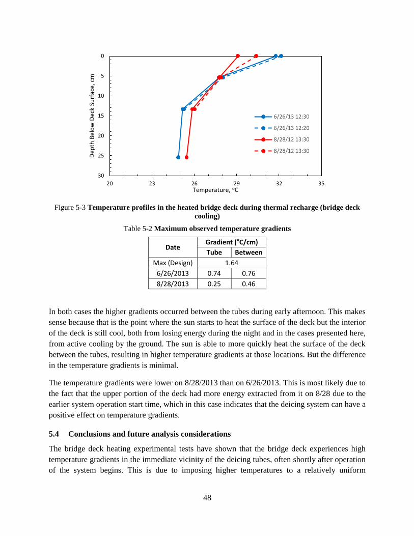
48
Figure 5-3 Temperature profiles in the heated bridge deck during thermal recharge (bridge deck
cooling)
Table 5-2 Maximum observed temperature gradients
Date Gradient (oC/cm)
Tube Between
Max (Design) 1.64
6/26/2013 0.74 0.76
8/28/2013 0.25 0.46
In both cases the higher gradients occurred between the tubes during early afternoon. This makes
sense because that is the point where the sun starts to heat the surface of the deck but the interior
of the deck is still cool, both from losing energy during the night and in the cases presented here,
from active cooling by the ground. The sun is able to more quickly heat the surface of the deck
between the tubes, resulting in higher temperature gradients at those locations. But the difference
in the temperature gradients is minimal.
The temperature gradients were lower on 8/28/2013 than on 6/26/2013. This is most likely due to
the fact that the upper portion of the deck had more energy extracted from it on 8/28 due to the
earlier system operation start time, which in this case indicates that the deicing system can have a
positive effect on temperature gradients.
5.4 Conclusions and future analysis considerations
The bridge deck heating experimental tests have shown that the bridge deck experiences high
temperature gradients in the immediate vicinity of the deicing tubes, often shortly after operation
of the system begins. This is due to imposing higher temperatures to a relatively uniform
0
5
10
15
20
25
30
20 23 26 29 32 35
Dep
th B
elo
w D
eck
Surf
ace,
cm
Temperature, oC
6/26/13 12:30
6/26/13 12:20
8/28/12 13:30
8/28/12 13:30

49
temperature profile. The highly localized effect of these temperature gradients make it difficult to
analyze the resulting stresses for several reasons:
On a small scale, the circulation tubes are often connected directly to the top layer of
reinforcement, which runs in the longitudinal and transverse directions. Because the
higher temperature gradients exist in the immediate vicinity of the deicing tubes, they
will also exist in the vicinity of the rebar reinforcement if the tubes are attached. Thus,
the typical assumption that a bridge deck is a homogenous concrete slab that behaves
according to modified properties that account for the respective volumetric percentages
of concrete and rebar is not valid. In terms of thermal properties, steel and concrete are
remarkably different. Furthermore, the circulation tubes are composed of a different
material (often some type of polymer based plastic), with different thermal properties and
add an additional level of complexity.
On a macro scale, resulting stresses will not only depend on temperature gradients in the
deck, but on the bridge deck restraint conditions.
However, despite these uncertainties a few preliminary conclusions can be drawn:
During moderate weather conditions, the highest temperature gradients observed were
well within design values. The extreme temperature gradients occurred during periods of
severe weather conditions, which do not occur very frequently throughout the year.
The severe temperature gradients often occurred due to changing the uniform temperature
gradient of the slab. This could be avoided by selecting a start time such that a uniform
temperature gradient does not exist in the slab. In the case of bridge deck heating, late
afternoon and early evening are often good times to turn on a system following a sunny
day as the top several centimeters of the deck will be warmer, meaning a less extreme
temperature gradient will be created in the immediate vicinity of the circulation tubes
when warm fluid is circulated.
Despite the extreme temperature gradients that occurred, they were relatively transient in
nature and did not exist for a very long period of time as the heat propagated from the
tubes throughout the deck.
In examining bridge deck cooling, which occurs during thermal recharge operations during the
summer, temperature gradients larger than the design values were not observed. In fact, it
appears from preliminary results that the circulation system can serve to reduce the temperature
gradients in the upper portion of the bridge deck. These effects are also less localized around the
tubes than those of bridge deck heating, and appear to be rather uniform in the longitudinal and
transverse bridge deck directions.

50
6. Finite difference analysis of heat exchange through geothermal piles
Two different numerical modeling approaches have been adopted in this research to model pile-
soil heat exchange. The first modeling approach utilizes finite difference solution technique. A
finite difference code developed by Ghasemi-Fare and Basu (2013a, 2013b, 2015) is used for
solving a system of partial differential equations which describe heat flow through heat carrier
fluid and heat conduction in soil and concrete. In the later part of this research, the first
generation FD model was extended to a more rigorous second generation model that can
essentially capture the effects of different design, operational and site-specific variables on time-
dependent variation of ground and circulation fluid temperature.
6.1 Annular cylinder model
Heat transfer through a concrete geothermal pile with an embedded U-shaped circulation tube is
first modeled using an annular cylinder approximation. Half of the pile is modeled exploiting the
approximately axisymmetric heat flow condition in the medium surrounding the pile (Figure
6-1a). Note that the location and arrangement of the circulation tubes within a geothermal pile
does not strictly satisfy the condition of an axisymmetric geometry. However, the diameter of the
circulation tube (heat source) is two orders of magnitude smaller than the expected thermal
influence zone surrounding the pile. Therefore, the assumption of axisymmetric heat conduction
in the media (i.e., concrete and soil) surrounding the heat source is not far from reality.
(a) (b)
Fluid within
circulation tube
Concrete pile
Soil
dz
rp
2rbR
rq
rq
Circulation fluid Concrete pile Soil
r
C o n s t a n t T e m p e r a t u r e
C o n s t a n t T e m p e r a t u r e
C
on
s
ta
nt
T
em
pe
r
at
ur
e
i+1, j
i+1, j+1i, j+1
R
i, j
z
Z
N
o F
l
ow
Origin O (fluid inlet point)
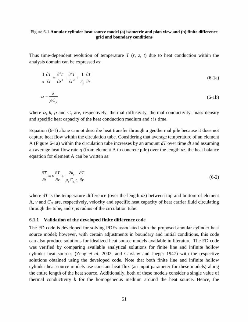
51
Figure 6-1 Annular cylinder heat source model (a) isometric and plan view and (b) finite difference
grid and boundary conditions
Thus time-dependent evolution of temperature T (r, z, t) due to heat conduction within the
analysis domain can be expressed as:
2 2
2 2
m
1 1
T T T T
t z r rr (6-1a)
p
k
C
(6-1b)
where , k, and Cp are, respectively, thermal diffusivity, thermal conductivity, mass density
and specific heat capacity of the heat conduction medium and t is time.
Equation (6-1) alone cannot describe heat transfer through a geothermal pile because it does not
capture heat flow within the circulation tube. Considering that average temperature of an element
A (Figure 6-1a) within the circulation tube increases by an amount dT over time dt and assuming
an average heat flow rate q (from element A to concrete pile) over the length dz, the heat balance
equation for element A can be written as:
f
c
f p t
2kT T Tv
t z C r r
(6-2)
where dT is the temperature difference (over the length dz) between top and bottom of element
A, v and Cpf are, respectively, velocity and specific heat capacity of heat carrier fluid circulating
through the tube, and rt is radius of the circulation tube.
6.1.1 Validation of the developed finite difference code
The FD code is developed for solving PDEs associated with the proposed annular cylinder heat
source model; however, with certain adjustments in boundary and initial conditions, this code
can also produce solutions for idealized heat source models available in literature. The FD code
was verified by comparing available analytical solutions for finite line and infinite hollow
cylinder heat sources (Zeng et al. 2002, and Carslaw and Jaeger 1947) with the respective
solutions obtained using the developed code. Note that both finite line and infinite hollow
cylinder heat source models use constant heat flux (an input parameter for these models) along
the entire length of the heat source. Additionally, both of these models consider a single value of
thermal conductivity k for the homogeneous medium around the heat source. Hence, the

52
following modifications are required in order for the developed FD code to capture the constant-
heat-flux condition at r = 2rt:
t2 t 2π
l
r r
qT
r r k
(6-3)
t
1, ,
21 2 1 t
2
1 12
T
r 2π
t
i j i j l
i r r i
i ir r
T TT q
r r r kT
r r r
(6-4)
where lq is the constant heat flux per unit length of the heat exchanger. Error! Reference
ource not found. shows that the developed FD code can successfully predict analytical heat
transfer solutions for finite line source (l
q = 100 Wm-1
, rb = 0.025 m, Lb = 5 m and Rb = rb/ Lb =
0.005; rb and Lb are, respectively, radius and length of the idealized heat source) and infinite
hollow cylinder source (l
q = 100 Wm-1
, rb = 0.3 m and Lb /rb = 100).
(a) (b)
Figure 6-2 Comparison between analytical solutions and results obtained using the developed Finite
Difference code (with appropriate modifications) for (a) finite line heat source (steady-state
solution) and (b) infinite hollow cylinder heat source (transient solution)
6.1.2 Analysis results
Analyses are performed using the developed FD code to quantify heat transfer through a 30-m-
long, 0.6-m-diameter (rp=0.3 m) geothermal pile under different thermal loading conditions. A
0 4000 8000 12000
Normalized time Fo =t/rb2
18
28
38
48
58
68
78
Te
mpera
ture
T (
°C)
adja
cen
t to
the h
eat sourc
e
Analytical (steady satate) solution for finite line source (Zeng et al. 2002)
Finite difference solution
ql=100Wm-1
k=1.5 Wm-1K-1
Tinitial=18 °C
z=2.5 mLb=5 m
rb=0.025 m
Rb=rb/Lb= 0.005
0 4 8 12
Normalized time Fo =t/rb2
18
20
22
24
26
28
30
32
Tem
pera
ture
T (
°C)
adja
cent to
the h
eat so
urc
e
Analytical (transient) solution for infinite hollow cylinder source
(Carslaw and Jaeger 1947)
Finite difference solution
ql=100Wm-1
k=2.3 Wm-1K-1
Tinitial=18 °C
rb=0.3 m
Lb/rb=100
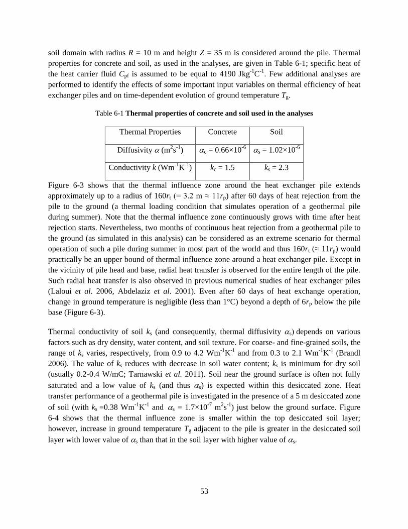
53
soil domain with radius R = 10 m and height Z = 35 m is considered around the pile. Thermal
properties for concrete and soil, as used in the analyses, are given in Table 6-1; specific heat of
the heat carrier fluid Cpf is assumed to be equal to 4190 Jkg-1
C-1
. Few additional analyses are
performed to identify the effects of some important input variables on thermal efficiency of heat
exchanger piles and on time-dependent evolution of ground temperature Tg.
Table 6-1 Thermal properties of concrete and soil used in the analyses
Thermal Properties Concrete Soil
Diffusivity (m2s
-1) c = 0.66×10
-6 s = 1.02×10
-6
Conductivity k (Wm-1
K-1
) kc = 1.5 ks = 2.3
Figure 6-3 shows that the thermal influence zone around the heat exchanger pile extends
approximately up to a radius of 160rt (= 3.2 m ≈ 11rp) after 60 days of heat rejection from the
pile to the ground (a thermal loading condition that simulates operation of a geothermal pile
during summer). Note that the thermal influence zone continuously grows with time after heat
rejection starts. Nevertheless, two months of continuous heat rejection from a geothermal pile to
the ground (as simulated in this analysis) can be considered as an extreme scenario for thermal
operation of such a pile during summer in most part of the world and thus 160rt (≈ 11rp) would
practically be an upper bound of thermal influence zone around a heat exchanger pile. Except in
the vicinity of pile head and base, radial heat transfer is observed for the entire length of the pile.
Such radial heat transfer is also observed in previous numerical studies of heat exchanger piles
(Laloui et al. 2006, Abdelaziz et al. 2001). Even after 60 days of heat exchange operation,
change in ground temperature is negligible (less than 1°C) beyond a depth of 6rp below the pile
base (Figure 6-3).
Thermal conductivity of soil ks (and consequently, thermal diffusivity sdepends on various
factors such as dry density, water content, and soil texture. For coarse- and fine-grained soils, the
range of ks varies, respectively, from 0.9 to 4.2 Wm-1
K-1
and from 0.3 to 2.1 Wm-1
K-1
(Brandl
2006). The value of ks reduces with decrease in soil water content; ks is minimum for dry soil
(usually 0.2-0.4 W/mC; Tarnawski et al. 2011). Soil near the ground surface is often not fully
saturated and a low value of ks (and thus s) is expected within this desiccated zone. Heat
transfer performance of a geothermal pile is investigated in the presence of a 5 m desiccated zone
of soil (with ks=0.38 Wm-1
K-1
ands = 1.7×10⁻⁷
m2s
-1) just below the ground surface. Figure
6-4 shows that the thermal influence zone is smaller within the top desiccated soil layer;
however, increase in ground temperature Tg adjacent to the pile is greater in the desiccated soil
layer with lower value of s than that in the soil layer with higher value of s.

54
Figure 6-3 Temperature (°C) profile in homogeneous ground surrounding a geothermal pile after 60
days of heat rejection
(b)
Figure 6-4 Temperature (°C) profile (after 60 days of heat rejection) around a geothermal pile
installed in ground with a top 5 m desiccated zone
0 0.5 1 1.5 2 2.5 3 3.5 4
Radial distance r (m)
35
30
25
20
15
10
5
0
De
pth
z (
m)
18
20
22
24
26
28
30
32
34
36
Tinlet=37 °C
Tinitial=18 °C
rt=0.02 m
rp= 0.3 m
L=15 mks=2.3 Wm-1K-1
kc=1.5 Wm-1K-1
v=0.1 ms-1
t=60 days
37
Te
mp
era
ture
sca
le (
°C)
0 0.5 1 1.5 2 2.5 3 3.5 4
Radial distance r (m)
35
30
25
20
15
10
5
0
De
pth
z (
m)
18
20
22
24
26
28
30
32
34
36
Tinlet=37 °C
Tinitial=18 °C
rt=0.02 m
rp= 0.3 m
L=15 mks=2.3 Wm-1K-1
kc=1.5 Wm-1K-1
v=0.1 ms-1
t=60 days
Te
mp
era
ture
sca
le (
°C)
37Desiccated zone;ks=0.38 Wm-1K-1

55
6.1.3 Effect of operational parameters
Velocity of fluid circulation through the embedded circulation tube and fluid temperature at the
inlet point are expected to play key roles on ground temperature response and energy exchange
efficiency of the pile-soil system. Hence, the effects of inlet fluid temperature Tinlet (which
implies thermal gradient based on the difference Δθ between inlet and initial ground
temperature) and fluid circulation velocity v on ground temperature response are investigated.
The effects of initial temperature difference Δθ (= Tinlet – Tinitial) and fluid circulation velocity v
on ground temperature Tg is shown in Figure 6-5. It is observed that at any given time t after the
start of the heat transfer operation, the thermal influence zone is independent of Δθ and v.
Ground temperature Tg within the thermal influence zone increases with increase in both Δθ and
v. Figure 6-6 shows (for v = 0.02 and 0.1 ms-1
) the variation of temperature T along depth z at
different radial distances; temperature gradient along depth (dT/dz) increases as v decreases.
Figure 6-5 (a)
1 5 9 13 17 21
Normalized radial distance r/rp
18
20
22
24
26
Gro
un
d t
em
pera
ture
Tg (
°C)
Tinlet=37°C (=19°C), t=12 days
Tinlet=37°C (=19°C), t=60 days
Tinlet=27°C (=9°C), t=12 days
Tinlet=27°C (=9°C), t=60 days
Tinitial=18 °C
rt=0.02 m
rp=0.3 m
L=30 mz=L/2ks=2.3 Wm-1K-1
kc=1.5 Wm-1K-1
v=0.1 ms-1

56
Figure 6-5 (b)
Figure 6-5 Variation of ground temperature Tg for different values of (a) initial temperature
difference θ (= Tinlet−Tinitial) and (b) fluid circulation velocity v
Figure 6-6 Effect of fluid circulation velocity v on temperature T along depth z
1 5 9 13 17 21
Normalized radial distance r/rp
18
20
22
24
26
Gro
un
d t
em
pera
ture
Tg (
°C)
v=0.1 ms-1, t=12 days
v=0.1 ms-1, t=60 days
v=0.02 ms-1, t=12 days
v=0.02 ms-1, t=60 days
=19°CTinlet=37 °C
Tinitial=18 °C
rt=0.02 m
rp=0.3 m
L=30 mz=L/2ks=2.3 Wm-1K-1
kc=1.5 Wm-1K-1
18 22 26 30
Temperature T (°C)
40
30
20
10
0
Dep
th z
(m
)
v=0.02 ms-1, r=rp
v=0.1 ms-1, r=rp
r=2rp r=0.5rp
Tinlet=37 °C
Tinitial=18 °C
rt=0.02 m
rp=0.3 m
L=30 mz=L/2ks=2.3 Wm-1K-1
kc=1.5 Wm-1K-1
r=rp
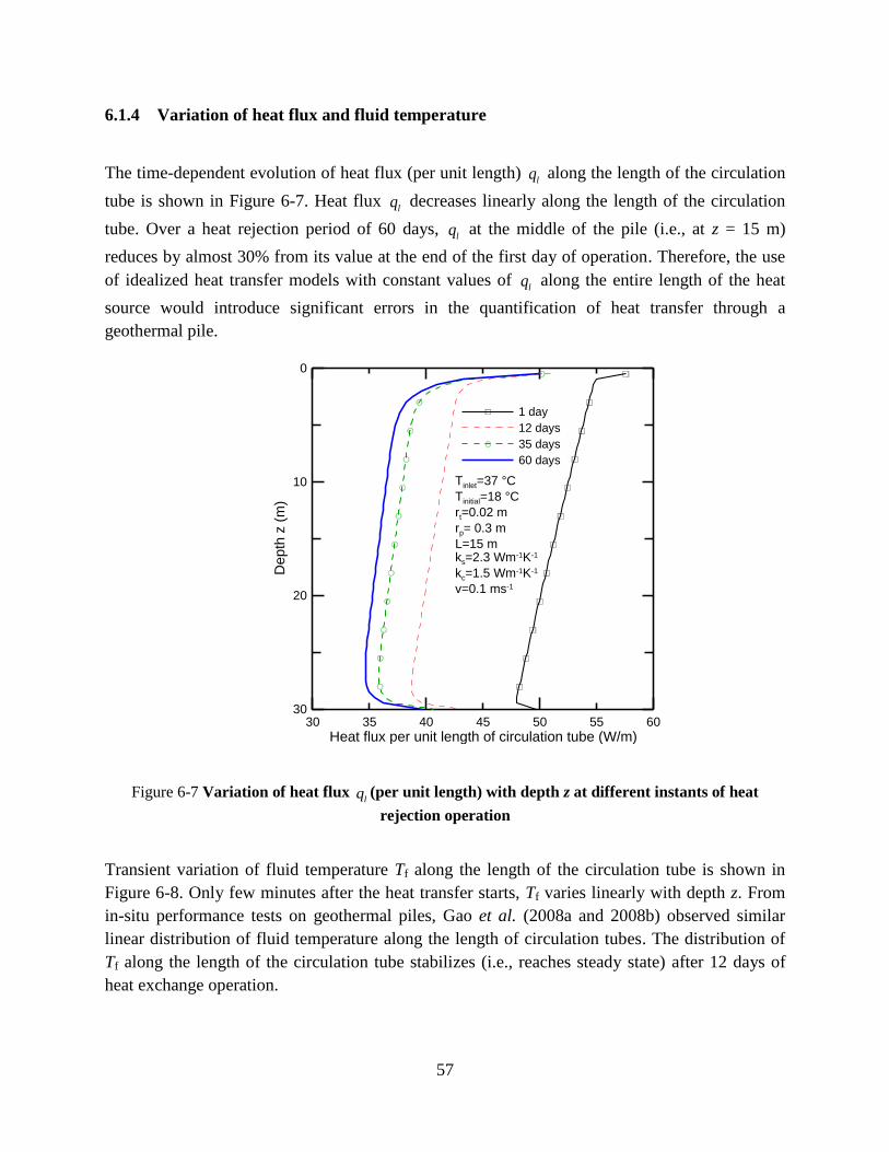
57
6.1.4 Variation of heat flux and fluid temperature
The time-dependent evolution of heat flux (per unit length) lq along the length of the circulation
tube is shown in Figure 6-7. Heat flux lq decreases linearly along the length of the circulation
tube. Over a heat rejection period of 60 days, lq at the middle of the pile (i.e., at z = 15 m)
reduces by almost 30% from its value at the end of the first day of operation. Therefore, the use
of idealized heat transfer models with constant values of lq along the entire length of the heat
source would introduce significant errors in the quantification of heat transfer through a
geothermal pile.
Figure 6-7 Variation of heat flux lq (per unit length) with depth z at different instants of heat
rejection operation
Transient variation of fluid temperature Tf along the length of the circulation tube is shown in
Figure 6-8. Only few minutes after the heat transfer starts, Tf varies linearly with depth z. From
in-situ performance tests on geothermal piles, Gao et al. (2008a and 2008b) observed similar
linear distribution of fluid temperature along the length of circulation tubes. The distribution of
Tf along the length of the circulation tube stabilizes (i.e., reaches steady state) after 12 days of
heat exchange operation.
30 40 50 6035 45 55
Heat flux per unit length of circulation tube (W/m)
30
20
10
0
Dep
th z
(m
)
1 day
12 days
35 days
60 days
Tinlet=37 °C
Tinitial=18 °C
rt=0.02 m
rp= 0.3 m
L=15 mks=2.3 Wm-1K-1
kc=1.5 Wm-1K-1
v=0.1 ms-1
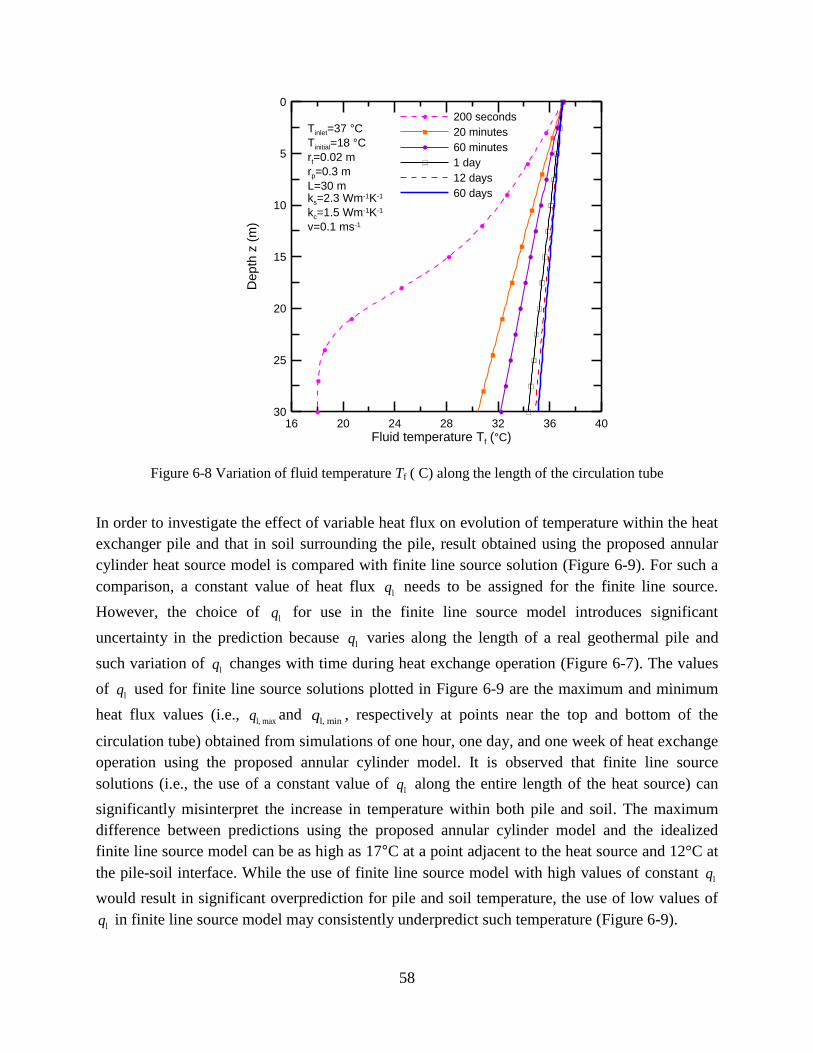
58
Figure 6-8 Variation of fluid temperature Tf ( C) along the length of the circulation tube
In order to investigate the effect of variable heat flux on evolution of temperature within the heat
exchanger pile and that in soil surrounding the pile, result obtained using the proposed annular
cylinder heat source model is compared with finite line source solution (Figure 6-9). For such a
comparison, a constant value of heat flux lq needs to be assigned for the finite line source.
However, the choice of lq for use in the finite line source model introduces significant
uncertainty in the prediction because lq varies along the length of a real geothermal pile and
such variation of lq changes with time during heat exchange operation (Figure 6-7). The values
of lq used for finite line source solutions plotted in Figure 6-9 are the maximum and minimum
heat flux values (i.e., l, maxq and
l, minq , respectively at points near the top and bottom of the
circulation tube) obtained from simulations of one hour, one day, and one week of heat exchange
operation using the proposed annular cylinder model. It is observed that finite line source
solutions (i.e., the use of a constant value of lq along the entire length of the heat source) can
significantly misinterpret the increase in temperature within both pile and soil. The maximum
difference between predictions using the proposed annular cylinder model and the idealized
finite line source model can be as high as 17°C at a point adjacent to the heat source and 12°C at
the pile-soil interface. While the use of finite line source model with high values of constant lq
would result in significant overprediction for pile and soil temperature, the use of low values of
lq in finite line source model may consistently underpredict such temperature (Figure 6-9).
16 20 24 28 32 36 40
Fluid temperature Tf (°C)
30
25
20
15
10
5
0
Dep
th z
(m
)
200 seconds
20 minutes
60 minutes
1 day
12 days
60 days
Tinlet=37 °C
Tinitial=18 °C
rt=0.02 m
rp=0.3 m
L=30 mks=2.3 Wm-1K-1
kc=1.5 Wm-1K-1
v=0.1 ms-1

59
(a) (b)
(c) (d)
Figure 6-9 Effect of variable heat flux on temperature within pile and soil at different times after the
start of heat exchange operation for (a) t = 4 days, (b) t = 12 days, (c) t = 35 days and (d) t = 60 days
6.2 U-tube model
A finite difference (FD) model has been developed at PSU to investigate the heat transfer from
the heat carrier fluid to the surrounding media considering a vertical plane that passes through
the pile and contains both branches of the U-shaped circulation tube embedded within the heat
exchanger pile (Ghasemi-Fare and Basu 2013a, 2013b, 2015; Ghasemi-Fare 2015). The model is
capable to predict the outlet fluid temperature as well as soil and concrete temperature. The
0.1 1 10 100
Normalized radial distance r/rp
18
23
28
33
38
43
48
53
58T
em
pera
ture
T (
°C)
Analysis using the proposed annular cylinder model
After 4 days
Tinlet=37 °C
Tinitial=18 °C
rt=0.02 m
rp=0.3 m
L=30 mz=L/2ks=2.3 W/mC
kc=1.5 W/mC
v=0.1 m/s
= 100 W/m
= 82 W/m
= 55 W/m
= 48 W/m
= 45 W/m
= 40 W/m
Prediction using finite line source model
After 1 hour
After 1 day
After 1 week
0.1 1 10 100
Normalized radial distance r/rp
18
23
28
33
38
43
48
53
58
Te
mp
era
ture
T (
°C)
Analysis using the proposed annular cylinder model
After 12 days
Tinlet=37 °C
Tinitial=18 °C
rt=0.02 m
rp=0.3 m
L=30 mz=L/2ks=2.3 W/mC
kc=1.5 W/mC
v=0.1 m/s
= 100 W/m
= 82 W/m
= 55 W/m
= 48 W/m
= 45 W/m
= 40 W/m
Prediction using finite line source model
After 1 hour
After 1 day
After 1 week
0.1 1 10 100
Normalized radial distance r/rp
18
23
28
33
38
43
48
53
58
Te
mp
era
ture
T (
°C)
Analysis using the proposed annular cylinder model
After 35 days
Tinlet=37 °C
Tinitial=18 °C
rt=0.02 m
rp=0.3 m
L=30 mz=L/2ks=2.3 W/mC
kc=1.5 W/mC
v=0.1 m/s
= 100 W/m
= 82 W/m
= 55 W/m
= 48 W/m
= 45 W/m
= 40 W/m
Prediction using finite line source model
After 1 hour
After 1 day
After 1 week
0.1 1 10 100
Normalized radial distance r/rp
18
23
28
33
38
43
48
53
58
Te
mp
era
ture
T (
°C)
Analysis using the proposed annular cylinder model
After 60 days
Tinlet=37 °C
Tinitial=18 °C
rt=0.02 m
rp=0.3 m
L=30 mz=L/2ks=2.3 W/mC
kc=1.5 W/mC
v=0.1 m/s
= 100 W/m
= 82 W/m
= 55 W/m
= 48 W/m
= 45 W/m
= 40 W/m
Prediction using finite line source model
After 1 hour
After 1 day
After 1 week

60
model simultaneously solves partial differential equations for (i) heat conduction within the
concrete pile and soil (ii) heat balance within the circulation tube and. Except than the
aforementioned partial differential equations, heat flow continuity equations should also be
considered to predict time dependent temperature evolution of the fluid, concrete, and soil. Two
individual heat sources are considered in the developed model. Schematic view of the domain is
presented in Figure 6-10. Temperature increments in any arbitrary point in the media due to both
downward and upward branches of U-tube can be calculated using:
2 2 2 2
1 1 , , , ,
in out in out
i
L RL L R R ij
i i j i jp ii ji i jQ Qz r r r r QC T Q
(6-5)
where Rr [= {r−0.5st−(rt+tt)}] and L
r [= {r+0.5st+(rt+tt)}] are radial distances measured,
respectively, from the center of the downward (left) and upward (right) branches of the
circulation tube, z is the distance between the top and bottom surfaces of the FD stencil, and
Cp are, respectively, mass density and specific heat capacity of the medium in which the FD
stencil is located. , ,
Lin out
i j i jQ Q and , ,
Rin out
i j i jQ Q are net heat flow into the stencil, respectively,
due to the left (designated by the letter L) and right (designated by the letter R) branches of the
circulation tube..
Considering the radial convection resistance of the fluid circulating inside the circulation tube,
heat balance equation for any element within a branch of the U-tube can be expressed as:
w
t
ppff
2
r r
kT T
t z C r
Tv
r (6-6)
where v is average velocity of fluid circulation and rt is inner radius of the circulation tube), f is
mass density of circulation fluid, Cpf is specific heat of circulation fluid, Tavg is the average fluid
temperature at any cross section and can be calculated as
t
avg 2
t 0
2r
m
T rvTdrv r
; vm is the mean fluid
velocity at the cross section under consideration. The variation of flow velocity at any depth
within the circulation tube is not considered in this study, therefore, v = vm.

61
Figure 6-10 Schematic domain of the numerical model developed at PSU
Coupling of equations (6-5) and (6-6) at the fluid–tube (PVC) interface [i.e. at r = ±(0.5st+tt),
±(0.5st+2rt+tt); tt is the thickness of the PVC tube] is achieved through heat flux continuity
condition imposed at the fluid-PVC interface.
f fm fw t
fluid-PVC interface
Th T T k
r
(6-7)
where kt is the thermal conductivity of the PVC tube.
Coupled solution of equations (6-5) and (6-6) can capture heat transport along the length of the
circulation tube branches and the heat conduction within the soil and the pile.
6.2.1 Finite difference formulation
Using an explicit solution scheme for two consecutive time steps, finite difference form of the
governing partial differential equation (6-5) can be written as:
Fluid inlet point Fluid outlet point
Z
Origin O
C o n v e c t i v e b o u n d a r y
C o n s t a n t t e m p e r a t u r e
b o u n d a r y
r
H e a t f l o w c o n t i n u i t y
i+1, j
i, j-1
i-1, j
i, j+1
Fluid within the pipe PVC tube RzPile radius rp
Circulation tube
with radius rt
Shank
distance st
SoilPile (Concrete)

62
L L R R, 1, , 1,
L L R R
, 1, , 1, 2
2 22 2 2( , )
1 1
2 2 2 21
i j i j i j i ji j i j i j i jr r r r r r r r
L L R Ri j
i i i i
T T T T
r r r r T
z
r r r rT
tr r r r
(6-8)
Combination of Equations (6-6)-(6-7) provides fluid temperature variation within a cross section
of the circulation tube at any depth. The finite difference form of the resulting equation is:
1
, , , 1 , 1, ,
pff
2( )
t t t t t t
i j i j i j i j i j i j
j ip
gk ttT T v T T T T
z C r r (6-9)
As values of thermal conductivity (and consequently, thermal diffusivity) of soil, concrete and
pipes are different, heat flow continuity conditions are required at the pipe-concrete interface (i.e.
at r = ± (0.5s ± rp); rp is the radius of the pipe and s is the shank spacing) and at the pile-soil
interface (i.e. at br r ; rb is the radius of the borehole heat exchanger).
The finite difference form of the heat flow continuity condition at the grout-soil interface is
presented below. Similar continuity condition is used at the pipe-concrete interface as well.
2 2 2 2
1 1
2 2
1 1
2 1 1
s 1 g 1
2 1 2 1
1 1
c s
1c s
2 2 2
1s 2 2 2
1 1
1
i i i i
i i
t t t t
i i i i
i i
i i i i
i i
t t
i i
i i i
r r r r
r r
T T T Tk r k r
r r r r Tk
r r r z
T T
t
k
r r
r r
k
2
g 2
2 2
1
2 2
1 1
i i
i i
Tk
z
r r
r r
(6-10)
Convective boundary condition is used for the top boundary of the analysis domain, and constant
temperature boundary condition is used for the left, right and bottom boundaries (Figure 6-10).
Convective boundary condition for the ground surface and constant temperature boundary for the
bottom side are defined in equations (6-11a) and (6-11b) respectively.

63
1
, ,
21, ,
, 2
, 1 ,
tg , ag
( )1
( )1 ( for ,) 0
t t
i j i j
t t
i j i j
i j
i
t t
i j i j t
i j
TT T t
r
T T
r r
T Th T R rT R z
z z
(6-11a)
initial for , T T R r R z Z (6-11b)
where htg is a convective heat transfer coefficient through the top boundary of the analysis
domain and Tag is the temperature of the medium above ground surface.
6.2.2 Stability condition
Time step size Δt that can be used in the FD formulation depends on the grid density. To avoid
solution instability, maximum time step used in the analyses was restricted to that derived using
Courant-Friedrichs-Lewy stability criterion (Courant et al. 1967). For the given problem, Δt is
decided based on the following expression:
f
p
f p
2 2
1
1
2
2
min
2
p
t
k
C r r
v
r z r rt
z
(6-12)
6.2.3 Verification
The accuracy of the finite difference model developed at PSU was studied by comparing the
numerical model predictions with the results obtained from the available analytical solution for a
finite line source (FLS) model (Zeng et al. 2002). The accuracy of the model for both short term
(a couple of hours) and long term (2 months of operation) was investigated using the analytical
solution. In order to compare the FD model a single value of thermal conductivity and diffusivity
is used for all the materials (soil, pile, and PVC tube).
In order to verify the model, the heat source was assumed to be the FLS model with length equal
to that of the pile placed along the center of the pile. An equivalent amount of constant power per
unit length ql (= Q/L; where Q is constant power injected at the inlet point and L is pile length) is
used in the FLS model. The fluid inlet temperature of the model depends on the output
temperature and the applied temperature differences calculated from the heat injection power.

64
in out 2
f f
t p
qT t T t
v r c (6-13)
Results from a trial analysis (for q = 2500 W and L = 25 m) using the developed FD model show
that, even for constant rate of power injection, heat rate varies from 55 Wm-1
at the inlet point to
45 Wm-1
at the outlet point of the circulation tube (Figure 6-11 a). Nevertheless, both short- and
long-term ground temperature response obtained from analysis using the FD model agrees well
with that predicted by the FLS model (Figure 6-11 b and Figure 6-11 c).
Figure 6-11 (a)
0 10 20 30 40 50 60 70 80 90 100 110
Heat rate per unit length ql (W/m)
25
20
15
10
5
0
De
pth
z (
m)
ql (t=1 day)
ql (t=5 days)
ql (t=10 days)
ql (t=15 days)
ql (FLS)
q = 2500 WTinitial=18°C
rt=0.01 m
st=0.05 m
L=25 mk=2.5 Wm-1K-1
v=0.3 ms-1
z=12.5 mkf=0.58 Wm-1K-1
f=0.725×10⁻³ Pa-s
ql
FLS=q
l,avg
inlet+q
l,avg
outlet

65
Figure 6-11 (b)
Figure 6-11 (c)
Figure 6-11 Comparison of the results obtained using FD and FLS models: (a) variation of ql with
depth, (b) radial variation of soil temperature at short-term (c) radial variation of soil temperature
at long-term
0 0.5 1 1.5 2
Radial distance r (m)
18
26
34
42
50
58
Gro
und
tem
pera
ture
Tg (
°C)
FLS - t = 1 hour
FLS - t = 6 hours
FLS - t = 24 hours
FDA - t = 1 hour
FDA - t = 6 hours
FDA - t = 24 hours
q=2500 W
q lFLS
=100 Wm-1
Tinitial=15°C
rt=0.01 m
st=0.05 m
L=25 mk=2.5 Wm-1K-1
v=0.3 ms-1
z=12.5 mkf=0.58 Wm-1K-1
f=0.725×10⁻³ Pa-s
Short term
Inlet side
Outlet side
0 2 4 6 8 10
Radial distance r (m)
18
26
34
42
50
58
Gro
und
tem
pera
ture
Tg (
°C)
FLS - t = 5 days
FLS - t = 15 days
FLS - t = 60 days
FDA - t = 5 days
FDA - t = 15 days
FDA - t = 60 days
q=2500 W
q lFLS
=100 Wm-1
Tinitial=15°C
rt=0.01 m
st=0.05 m
L=25 mk=2.5 Wm-1K-1
v=0.3 ms-1
z=12.5 mkf=0.58 Wm-1K-1
f=0.725×10⁻³ Pa-s
Long term
Inlet side
Outlet side

66
6.2.4 Comparison with published field test data
The developed FD model is also verified by comparing model predictions with recorded field
test data reported by Geo et al. (2008a and 2008b), Jalaluddin et al. (2011), Javed and Fahlen
(2011), and Abdelaziz (2013). The short-term thermal test reported by Gao et al. (2008a, and
2008b) on a 25-m-long geothermal pile with an embedded circulation tube (with radius rt=1cm)
is simulated using the FD model. Boundary conditions and values of different input parameters
(ks = 1.3 Wm-1
K-1
, αs = 5.86×10⁻⁷
m2s
-1, kc = 1.63 Wm
-1K
-1 and αc = 7.78×10
-7 m
2s
-1, f =
0.725×10⁻³
Pa-s, Tinitial = 18.2 °C, Tinlet = 35.13 °C and t = 3 hours) are adopted from Gao et al.
(2008a, and 2008b). Figure 6-12 shows that the outlet temperature Toutlet predicted using the
developed FD model compares very well with the recorded field data. Difference between
recorded field data and predicted value of Toutlet is only 0.06 °C. Figure 6-12 also shows that the
annular cylinder model described in Chapter 3 underpredicts fluid temperature along the length
of the circulation tube because the interaction between two branches of the tube is not considered
in the annular cylinder model. In absence of any recorded temperature data along the length of
the circulation tube, only the predicted distribution of fluid temperature along the circulation tube
is shown in Figure 6-12. The predicted linear variation of fluid temperature along the length of
the circulation tube is consistent with fluid temperature variation reported by Gao et al. (2008a,
and 2008b).
Jalaluddin et al. (2011) conducted field thermal performance tests on a 20-m-long steel
geothermal pile filled with silica sand. Different configurations of circulation tubes (single U-
tube, double-tube and multi-tube) were used in the field study. Results obtained for the single U-
shaped circulation tube (with inner radius rt = 1.3 cm) is used to gage the prediction capability of
the FD model. Field tests with two different values of fluid circulation (flow) rate qf = 6.67×10⁻⁵
and 1.33×10⁻⁴
m3s
-1 (corresponding to fluid circulation velocity v = 0.126 and 0.251 ms
-1,
respectively) are simulated using the FD model. All input parameters (rt = 0.013 m, ks = 1.2 Wm-
1K
-1, kf = 0.58 Wm
-1K
-1, f = 0.798×10
-3 Pa-s, Tinitial = 18 °C, Tinlet = 26.5 °C for qf = 3.33×10
-5
m3s
-1, and Tinlet = 26.3 °C for qf = 1.33×10
-4 m
3s
-1) are adopted based on the information provided
in Jalaluddin et al. (2011). The thermal conductivity of the grout (silica sand), as reported by
Jalaluddin et al. (2011), is used as the value of kc (= 1.4 Wm-1
K-1
). Figure 6-13 shows that values
of outlet fluid temperature Toutlet obtained from FDAs at both transient and steady state are in
good agreement with field data reported by Jalaluddin et al. (2011). The maximum difference
observed between recorded and predicted values of Toutlet is within 0.5% (0.08 °C, and 0.12 °C
temperature differences, respectively, for 8 and 4 lit/minutes).

67
Figure 6-12 Comparison of FD model prediction with circulation fluid temperature reported by Gao
et al. (2008a, and 2008b)
Figure 6-13 Prediction of fluid outlet temperature during the first day of operation of a geothermal
pile in field (Jalaluddin et al. 2011)
26 28 30 32 34 36
Fluid temperature Tf (°C)
30
25
20
15
10
5
0
De
pth
z (
m)
Field test results
Finite difference analysis
Annular cylinder model presented in Chapter 3
Tinlet=35.13 °C
Tinitial=18.2 °C
rt=0.01 m
rp=0.3 m
L=25 mks=1.3 Wm-1K-1
kc=1.628 Wm-1K-1
v=0.3 ms-1
f=0.725×10⁻³ Pa-s
0 5 10 15 20 25
Time (hr)
18
20
22
24
26
28
30
Flu
id o
utlet te
mpera
ture
To
utle
t (°C
)
Jalaluddin et al. 2011
qf=1.3310-4 m3s-1 (=8 liter/minutes)
FDA, qf=1.3310-4 m3s-1 (=8 liter/minutes)
Jalaluddin et al. 2011
qf=6.6710-5 m3s-1 (=4 liter/minutes)
FDA, qf=6.6710-5 m3s-1 (=4 liter/minutes)
Tinlet=26.4 °C, for qf=6.6710-5 m3/s
Tinlet=26.3 °C, for qf=1.3310-4 m3/s
Tinitial=18 °C
rt=0.013 m
tt=0.004 m
rp=0.09 m
L=20 mks=1.2 Wm-1K-1
kc=1.4 Wm-1K-1
kf=0.58 Wm-1K-1
f=0.798×10⁻³ Pa-s

68
6.2.5 Temperature Difference T between Inlet and Outlet Points
To investigate the amount of power output obtained from the ground and estimate the thermal
influence zone a heat exchange pile with real dimensions were considered in this research. A 25-
m-long, 0.6-m-diameter concrete geothermal pile with an embedded U-shaped circulation tube
was analyzed using the FD model described in this paper. A cylindrical soil domain (radius R =
12 m and depth Z = 30 m) with the pile in its center was considered for all analyses. Few trial
analyses were performed (with different boundary distances) to ensure that the constant
temperature boundary condition at the far boundaries was valid. An initial simulation, hereafter
referred to as base analysis, was performed using a set of expected values for model input
parameters (Table 6-2).
Temperature contour around the heat exchanger pile after 60 days of heat rejection from the pile
to the surrounding ground is presented in Figure 6-14.
Table 6-2 Input parameters used for base analysis
Parameters Value
Fluid circulation velocity v = 0.1 m/s
Convective heat transfer coefficient (from ground
surface) hg = 5 W/(m
2K)
Convective heat transfer coefficient (from top of the pile) hp = 0.01 W/(m2K)
Initial temperature Tinitial = 18 ̊ C
Inlet temperature Tinlet = 35 ̊ C
Length of each vertical branch of the circulation tube Lt = 24.8 m
Mass density of heat carrier fluid f = 1000 kg/m3
Pile length L = 25 m
Pile radius rp = 0.30 m
Radius of circulation tube rt = 0.02 m
PVC tube thickness tt = 6 mm
Shank distance (i.e., center-to-center distance between
two branches of the circulation tube) st= 40 cm
Specific heat of heat carrier fluid Cpf = 4190 J/(kgK)
Temperature in the medium above ground surface agT = 23 ̊C
Thermal conductivity of concrete kc = 1.7 W/(mK)
Thermal conductivity of soil ks = 2.5 W/(mK)
Thermal conductivity of PVC tube kt = 0.41 W/(mK)
Thermal diffusivity of concrete c = 0.9×10⁻⁶
(m2/s)
Thermal diffusivity of soil s = 1.4×10⁻⁶
(m2/s)
Thermal diffusivity of PVC tube t = 0.284×10⁻⁶
(m2/s)
Dynamic viscosity of fluid f = 0.725 m Pa. s
Thermal conductivity of fluid kf = 0.58 W/(mK)

69
Figure 6-14 Temperature contour (in °C) after 60 days of heat rejection from a geothermal
pile
The amount of heat transfer through a geothermal pile is related to the temperature difference T
(= Tinlet−Toutlet) between inlet and outlet points of the circulation tube. Error! Reference source
ot found. shows the variation of T with both real and normalized time expressed by Fourier
number Fo (= st/rt2). Temperature difference T, and thus the heat transfer rate, reduces sharply
within a very short period of time (approximately 1 day) after the heat transfer starts and reaches
nearly a constant value after 20 days of continuous heat rejection. Pile (concrete) and soil
temperature increases with time as heat is rejected from heat carrier fluid to the surrounding
media. Such temperature increase in the medium surrounding the heat source causes reduction in
temperature gradient (heat flux) between the heat source and the medium surrounding it. The
reduction in temperature gradient deters the rate of heat transfer from the heat carrier fluid and
thus, temperature Toutlet at the fluid outlet point increases. Consequently, for a constant value of
inlet temperature Tinlet, T reduces with time and reaches a nearly constant value at a certain time
(= 20 days for base analysis) after heat rejection starts.
-6 -5 -4 -3 -2 -1 0 1 2 3 4 5 6
Radial distance (m)
30
28
26
24
22
20
18
16
14
12
10
8
6
4
2
0
De
pth
z (
m)
Te
mp
era
ture
sca
le (
°C)
18
19
21
23
25
27
29
31
33
34
35
Tinlet=35°C
Tinitial=18°C
rt=0.02 m
rp=0.3 m
tt=0.006 m
v=0.1 ms-1
L=25 mks=2.5 Wm-1K-1
Kc=1.7 Wm-1K-1
kt=0.41 Wm-1K-1
kf=0.58 Wm-1K-1
f=0.725×10⁻³ Pa S
t=60 days

70
Regression analysis is performed to describe a simple mathematical form for calculation of Tb,
i.e., the value of T (in °C) as obtained from the base analysis, as a function of time t (in hours).
Error! Reference source not found. (a) shows that Equation (6-14) can successfully predict
result from the base analysis with a coefficient of determination R2
= 0.99.
0 2
b
.14.9
tT t (6-14)
Note that Equation (6-14) is valid only for the set of input parameters used in the base analysis.
The value of T is expected to vary for any other combination of design, operational and site-
specific parameters such as fluid circulation velocity v, radius of circulation tube rt, pile radius
rp, initial temperature difference (=Tinlet−Tinitial), thermal conductivity of concrete kc, and
thermal conductivity of soil ks. Considering individual effects of the above parameters on T, the
following general expression is proposed for T:
N
Nb
N Nb
a
xT t T t
x
(6-15)
where N is an index that indicates total number of important input parameters (for this study N =
6), xN takes the value of Nth
input parameter (e.g., v, , ks, kc, rt, and rp), xNb is the base value of
the Nth
input parameter (as reported in Table 6-2), and aN is a regression coefficient for the Nth
input parameter. In order to obtain the unknown coefficients aN in Equation (6-15), additional
FDAs are performed by varying one input parameter at a time while all other input parameters
are kept constant at their base values reported in Table 6-2. The expression for aN for each input
variable xN is determined through regression analyses of results obtained from these additional
FDAs.
The resulting closed form expression for ΔT becomes:
51
0
3 4 62
pc s t
0.1 17 1.7 2.5 0.3 0.02
a
aa a aa ark k rv
T tt A
(6-16)
The expressions for regression coefficients A, a0, a1, a2, a3, a4, a5 and a6 in Equation (6-16) are
summarized in Table 6-3.

71
Table 6-3 Regression coefficients for different input variables
Coefficients Turbulent (t is in hours) Laminar (t is in hours)
A 4.9 4.9
a0 −0.12 −0.12
1a −0.9 −0.7
2a 1 1
3a 0.35 0.02ln t 0.35 0.02ln t
4a 0.07 0.07ln t 0.07 0.07ln t
5a s pc0.05 0.01ln1.4 0.37
rk kt s pc0.05 0.01ln
1.4 0.37
rk kt
6a 1.15 0.05ln t 0.95 0.05ln t
6.2.6 Geothermal Power Output
The total amount of heat exchange between a geothermal pile and ground over a certain period of
thermal operation of the pile is defined as the energy output. Mathematically, the rate of energy
extraction or rejection P(t) (or power output) can be expressed as:
f pf
2
tp f rP t mC T t v C T t (6-17)
Note that fluid circulation velocity v and radius of circulation tube rt affect both m and T(t).
Therefore, the individual effects of v and rt on P(t) should be investigated separately. Although
some field studies quantified the effect of circulation flow rate qf (Gao et al. 2008a and 2008b,
and Jalaluddin et al. 2011) on energy extraction (or rejection) rate P(t), none of those studies
could conclusively differentiate individual effects of v and rt on P(t). The circulation velocity v
reversely affects m and T(t) in Equation (6-17); an increase in v increases m but reduces T(t).
Figure 6-15(a) shows, for a set of input parameters, that power output (at time t= 7 days) per unit
length of the pile increases with an increase in v and reaches to a constant value beyond a
threshold value of v (= 0.3 ms-1
) that can be designated as an efficient circulation velocity for
geothermal pile operation. P increases with increase in circulation tube radius rt, and it is
interesting to note that the value of efficient circulation velocity is independent of the value of rt.
Figure 6-15(b) shows power output (at time t = 7 days) per unit length of a geothermal pile as
obtained from FDAs with a constant circulation flow rate qf = 6.28×10⁻⁴
m3s
-1 (= 37.7
liter/minute). For a constant circulation flow rate qf, different combinations of v and rt can result
in an increase (or decrease) in energy extraction (or rejection) rate. It is evident from Figure
6-15(b) that for a constant flow rate qf, P increases as rt increases, and thus, the effect of rt on P
is higher than that of v.

72
(a)
(b)
Figure 6-15 Effects of circulation tube radius rt and fluid circulation velocity v on power output: (a)
variable circulation flow rate qf and (b) constant circulation flow rate qf
0 0.2 0.4 0.6 0.8
Fluid circulation velocity v (m/s)
20
30
40
50
60
70
80
Pow
er
outp
ut pe
r u
nit le
ngth
of th
e p
ile P
/L (
W/m
)
rt= 3 cm
rt= 2 cm
rt= 1 cm
Turbulentflow
Turbulentflow
Turbulentflow
All other input parameters are sameas used in the base analysis (Table 6-2)
t = 7 days
0 0.02 0.04 0.060.01 0.03 0.05
Radius of circulation tube rt (m)
10
30
50
70
90
110
20
40
60
80
100
Po
we
r o
utp
ut
pe
r u
nit le
ng
th o
f th
e p
ile P
/L (
W/m
)
rt= 1 cm, v=2 ms-1
rt= 2 cm, v=0.5 ms-1
rt= 3 cm, v=0.22 ms-1
rt= 4 cm, v=0.125 ms-1
qf = 6.2810-4 m3s-1 (=37.7 liter/minute)
All of them are turbulent flow
All other input parameters are sameas used in the base analysis (Table 6-2)
rt= 5 cm, v=0.08 ms-1
t = 7 days

73
The effect of flow characteristic (laminar or turbulent) on the amount of heat loss within the
circulation fluid is also studied in this research (Figure 6-16). Figure 6-16 shows fluid
temperature variation within a cross section (at the middle of the geothermal pile) of the inlet
branch of the circulation tube. The high value of convective heat transfer coefficient in case of a
turbulent flow results in minimal heat loss within the circulation tube; however, this is not the
case for a laminar flow condition, which exhibits as much as a 10% (3.25°C) reduction of fluid
temperature between the centerline and inside wall of the circulation tube.
Figure 6-16 Fluid temperature variations (within a cross section of circulation tube) with flow
characteristics
6.2.7 Closed-form expression to predict power output
The equations proposed for calculation of T(t) [i.e., Equation (6-16) in combination with Table
6-3] can be used in conjunction with Equation (6-17) to predict energy output over a certain
period of time of operation of a geothermal pile. Figure 6-17 compares power output (per unit
length of the pile) values obtained from several FDAs (performed with different combinations of
input parameters) and those predicted using proposed Equations (6-16), (6-17) and Table 6-3.
The proposed equations can successfully predict (with a maximum difference of less than 10%)
power output values for both short- and long-term operation (respectively, for t = 12 h and 60
days) of a geothermal pile with U-shaped circulation tube.
-0.02 -0.01 0 0.01 0.02
Radial distance from the PVC tube center
30
31
32
33
34
35
36
Flu
id te
mp
era
ture
Tf (
°C)
v=0.02 ms-1
v=0.07 ms-1
v=0.10 ms-1
v=0.30 ms-1
v=0.50 ms-1
Tinlet=35°C
Tinitial=18°C
rt=0.02 m
rp=0.3 m
L=25 mtt=0.006 m
ks=2.5 Wm-1K-1
kc=1.7 Wm-1K-1
kt=0.41 Wm-1K-1
kf=0.58 Wm-1K-1
f=0.798×10⁻³ Pa-s
Inlet tubez=L/2 t=5 days
Laminar flow
Turbulent flow
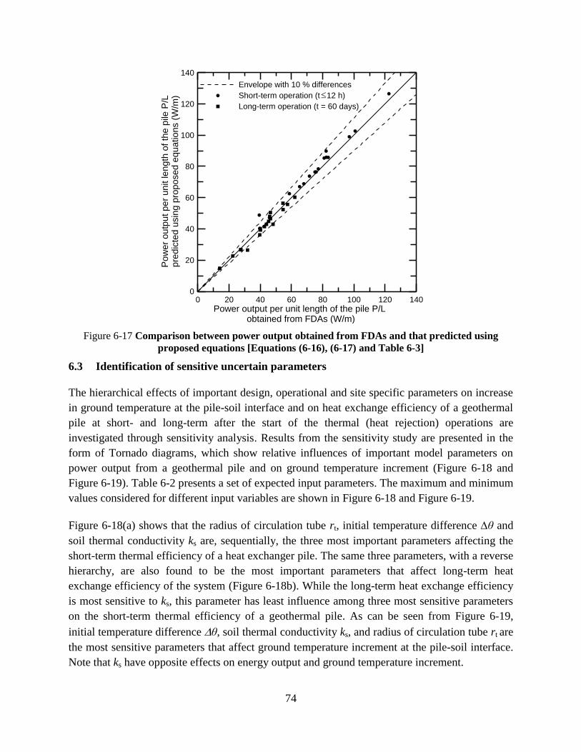
74
Figure 6-17 Comparison between power output obtained from FDAs and that predicted using
proposed equations [Equations (6-16), (6-17) and Table 6-3]
6.3 Identification of sensitive uncertain parameters
The hierarchical effects of important design, operational and site specific parameters on increase
in ground temperature at the pile-soil interface and on heat exchange efficiency of a geothermal
pile at short- and long-term after the start of the thermal (heat rejection) operations are
investigated through sensitivity analysis. Results from the sensitivity study are presented in the
form of Tornado diagrams, which show relative influences of important model parameters on
power output from a geothermal pile and on ground temperature increment (Figure 6-18 and
Figure 6-19). Table 6-2 presents a set of expected input parameters. The maximum and minimum
values considered for different input variables are shown in Figure 6-18 and Figure 6-19.
Figure 6-18(a) shows that the radius of circulation tube rt, initial temperature difference θ and
soil thermal conductivity ks are, sequentially, the three most important parameters affecting the
short-term thermal efficiency of a heat exchanger pile. The same three parameters, with a reverse
hierarchy, are also found to be the most important parameters that affect long-term heat
exchange efficiency of the system (Figure 6-18b). While the long-term heat exchange efficiency
is most sensitive to ks, this parameter has least influence among three most sensitive parameters
on the short-term thermal efficiency of a geothermal pile. As can be seen from Figure 6-19,
initial temperature difference θ, soil thermal conductivity ks, and radius of circulation tube rt are
the most sensitive parameters that affect ground temperature increment at the pile-soil interface.
Note that ks have opposite effects on energy output and ground temperature increment.
0 20 40 60 80 100 120 140Power output per unit length of the pile P/L
obtained from FDAs (W/m)
0
20
40
60
80
100
120
140
Po
wer
outp
ut p
er
un
it le
ng
th o
f th
e p
ile P
/Lp
red
icte
d u
sin
g p
rop
ose
d e
qu
atio
ns (
W/m
)
Envelope with 10 % differences
Short-term operation (t 12 h)
Long-term operation (t = 60 days)

75
(a)
(b)
Figure 6-18 Hierarchy of model parameters in affecting thermal efficiency of a geothermal pile: (a)
after 12 hours of operation (short-term) and (b) after 60 days of operation (long-term)
35 65 95 12550 80 110 140
Power output per unit length of the pile P/L (W/m)
= 22°C
ks=4.0 W/mC
= 9°C
ks=0.4 W/mC
rt=0.04 mrt=0.01 m
kc=2.0 W/mCkc=1.3 W/mC
v=0.5 m/sv=0.02 m/s
rp= 0.6 m rp= 0.15 m
From base analysis with input parameters
reported in Table 6-2
Short-term (t= 12 hours)
10 30 50 7020 40 60
Power output per unit length of the pile P/L (W/m)
= 22°C
ks=4.0 W/mC
= 9°C
ks=0.4 W/mC
rt=0.04 mrt=0.01 m
kc=2.0 W/mCkc=1.3 W/mC
v=0.5 m/sv=0.02 m/s
rp= 0.6 m rp= 0.15 m
From base analysis with input parameters
reported in Table 6-2
Long-term (t= 60 days)

76
Figure 6-19 Hierarchy of model parameters in affecting ground temperature increment at the pile-
soil interface after 60 days of thermal (heat rejection) operation
6.4 Summary and conclusion
Results from finite difference analyses presented in this chapter show that fluid circulation
velocity and radius of circulation tube independently affect energy output from a geothermal
pile. Beyond a short time after the start of heat transfer, thermal conductivity of concrete does
not have any significant effect on heat exchange through geothermal piles; however, the effect of
soil thermal conductivity on heat transfer efficiency increases with time. The effect of pile radius
on energy output depends on the ratio ks/kc; increase in pile radius increases heat exchange
efficiency for ks/kc < 1; the reverse is true when ks/kc > 1. A set of equations is proposed which
can be used to calculate power output from a geothermal pile for any practical set of input
variables. Comparison of heat loss within the fluid for laminar and turbulent flow shows that heat
loss within the circulation tube is relatively higher in laminar flow and consequently thermal
resistivity of fluid convection is higher in laminar flow. It is also evident from the results
presented in this chapter that an increase in circulation velocity results in an increase in the
harvested geothermal energy. Nevertheless, fluid circulation at higher velocity would require
more electric power; therefore, optimum circulation fluid velocity would eventually depend on
power efficiency of the circulation heat pump.
Effects of different design, operational, and site-specific variables on heat exchange efficiency of
geothermal piles must be quantified for reliable and efficient design of geothermal piles.
Although past studies focused on different aspects of heat exchange behavior of geothermal
0 4 8 12 16
Ground temperature increment (°C)
= 22°C
ks=4.0 W/mC
= 9°C
ks=0.4 W/mC
rt=0.04 mrt=0.01 m
kc=2.0 W/mCkc=1.3 W/mC
v=0.5 m/sv=0.02 m/s
rp= 0.6 m rp= 0.15 m
From base analysis with input parameters
reported in Table 6-2
Long-term (t= 60 days)

77
piles, no theoretical or experimental studies have yet comprehensively quantified the relative
variance of heat exchange efficiency and ground temperature increments due to individual or
combined variation of different design, operational, and site specific parameters (Yavusturk
1999, Hamada et al. 2007, Gao et al. 2008a, and 2008b, Nam et al. 2008, Lamarche et al. 2010,
McCartney et al. 2010, Abdelaziz et al. 2011, Suryatriyastuti et al. 2012, Rouissi et al. 2013,
Ghasemi-Fare and Basu 2013a, 2013b, Ghasemi-Fare et al. 2014, and Jalaluddin et al. 2011).
Sensitivity and reliability analyses show that thermal conductivity of soil, initial temperature
difference between ground and circulation fluid, and radius of circulation tube are sequentially
three most important parameters that affect long-term heat exchange performance of a
geothermal pile.
7. Finite element analysis of heat exchange through geothermal piles
The second numerical modeling approach utilizes a finite elements (FE) simulation environment,
COMSOL Multiphysics™ (COMSOL, 2013). Ozudogru et al. (2014a, 2014b) discusses the
modeling methodology in detail along with the validation of the model. This numerical model
utilizes 1D linear elements for simulating the fluid flow and heat transfer inside the circulation
tubes, which in turn is fully coupled with the 3D geometry using the temperature field at the pipe
exterior surface. The model can simulate the 3D transient and steady-state heat and mass
transport processes in the borehole and heat exchanger pile with satisfactory accuracy and
minimal computational effort.
7.1 Model development
The FE model considers several components of the GHE. These include the fluid in the pipes,
the pipes, the grout, and the soil surrounding the heat exchanger. The lateral and bottom extents
of the model are selected such that no thermal interaction occurs across the external boundaries.
The diameter of the pipe elements is taken equal to the pipe outside diameter and these elements
are identified as ‘pseudo pipes’. The actual physical representation of the pipes and the circulated
fluid is modeled using linear elements that cross between the center-axes of pseudo pipes in each
individual loop. Two dimensional elements are generated on a horizontal plane at the ground
surface for all the model components and extruded downward to the bottom extent of the model.
With the help of the linear pipe elements, the extrusion of the horizontal plane allows the
creation of continuous line elements by establishing a connection between downward and
upward pipes at the base of the GHE. Figure 7-1 provides more insight into the linear pipes and
the pseudo pipe approach, presenting the 3D extruded geometry.

78
Figure 7-1 The 3D geometry showing the linear and pseudo pipe elements
The model utilizes swept finite element meshing in the vertical direction, and the mesh is
optimized to minimize the number of elements. However, the reduction should not be done at the
expense of obtaining numerical results with poor accuracy. Prior experience shows that, mesh
refinement is required near the ground surface, soil/rock layer interfaces and the base of the heat
exchanger, where larger vertical temperature gradients reside. Minimum refinement is necessary
in mid-layers, where vertical temperature gradients are negligible. A similar meshing technique
was used in a study by Marcotte and Pasquier (2008). In vertical GHE applications, since the
heat transfer is predominantly in the radial direction and the vertical heat flow in the system is
insignificant, it is a reasonable approach to distribute the swept mesh on the vertical axis with
refinements only close to layer interfaces, or the depths where the extrusion of the 2D geometry
was stopped. This procedure leaves coarser vertical mesh inside the soil layers. There may be
exceptions to this approach in certain cases, such that, the first several meters below the ground
surface should also be refined if the vertical temperature gradient caused by temperature
variations near the ground surface will be considered in the model. The overall finite element
mesh of a GHE with double loop configuration is shown in Figure 7-2.

79
Figure 7-2 Overall finite element mesh of a GHE with a double loop configuration
7.2 Modifications
The FE model addresses the simulation of a GHE system by considering two problems: (1) the
time dependent heat transfer problem in the volumetric domains, which is solved by calculating
the temperature in each finite element mesh node; (2) the transient fluid flow and forced
convection problems in the pipes, solved by evaluating the temperatures of the fluid and the pipe
wall along the pipe axis. In the solid domains such as pseudo pipes, grout, and soil, pure
conductive heat transfer is anticipated which is governed by the following equation assuming
that there is no internal heat generation:
0p
Tc T
t
k (7-1)
Equation 7-1 is solved for temperature, T, making use of the temperature coupling between the
solid domains and the linear pipe elements. Boundary conditions designate the behavior of the
numerical model during runtime and are used to build the sparse matrix solved thereafter for
estimating the temperature changes. Either no heat flux (insulation – Neumann), or prescribed
5.15 m5 m
100 m
0.15 m

80
temperature (Dirichlet) boundary condition should be specified for the lateral and the bottom
limits of the model. For the former case, it must be ensured that there is no temperature change at
these boundaries while for the latter case, the heat flux on these boundaries must be zero
throughout the runtime of the model. This can be achieved by setting the extent of the model at
distances where heat exchange operations essentially have no effect. The Dirichlet boundary
condition can only be used if the initial temperature of the ground is selected as a single value for
all depths. For models with symmetrical geometry, no heat flux boundary condition is used on
the symmetry plane.
The fluid flow and heat transfer problem in the pipes is physically modeled using linear
elements, reducing the 3D flow problem to 1D. Modeling pipes as curves in 2D or 3D provides
great advantage in computational efficiency over meshing and computing 3D pipes with finite
diameter. The pipe flow problem is determined by solving the momentum and continuity
equations given by Barnard et al. (1966). Heat transfer problem in the pipes is governed by the
energy equation for an incompressible fluid flowing in a pipe:
3f pi
f pi f f pi f pi f2
p p D wall
h
ATA c A c T A k T f q
t d
u u
(7-2)
The second term on the right hand side corresponds to friction heat dissipated due to viscous
shear. The radial heat transfer from the surroundings into the pipe is given by:
¢qwall
=2p
2
Nu kf
+ln d
podpi( )
kp
Text
-T( ) (7-3)
The Darcy friction factor in Equation 7-2 accounts for the continuous pressure drop along a pipe
segment due to viscous shear, and it is estimated using the Churchill (1997) equation. Nusselt
number is defined as the ratio of convective to conductive heat transfer across a boundary. For
turbulent flow conditions, Nusselt number can be estimated using the correlation developed by
Gnielinski (1976).
The external temperature outside of the pipes, Text corresponds to the temperature field computed
in the volumetric domains that provides heat transfer coupling to the volumetric domains,
considering the pipes as a line heat source. However, there is a limitation of this approach. Since
the pipes are made of linear elements, the outer pipe wall temperature is coupled to the
temperature field of the volumetric domains located at the pipe axis. This introduces estimation
errors, because the temperature field of the volumetric domains to be coupled should be located
at a distance of pipe outside radius from the pipe axis. Another downside of this simplification is
that, it does not account for the heat capacity of the pipes. A ‘pseudo pipe’ approach was

81
developed as shown in Figure 7-1 to overcome these issues. The diameter of these cylindrical
solid domains is equal to the pipe outside diameter. The assigned material properties are selected
to ensure an accurate temperature coupling, while accounting for the heat capacity of the pipes,
as well.
7.3 Model Performance
The FE model was validated using data recorded during one of the field thermal conductivity
tests presented by Abdelaziz (2013). The test site was located at the Virginia Tech geotechnical
testing facility. Four heat exchanger piles and a reaction pile were installed at the site and several
thermal conductivity and thermo-mechanical loading tests were performed. Two types of thermal
conductivity tests were conducted at the test site: (1) in accordance with ASHRAE method
(Kavanaugh et al. 2001) and (2) following the Dutch perspective (Witte et al. 2002).
During the ASHRAE tests, the circulation fluid was heated with a constant heat rate using the
electric heaters located at the testing trailer. Even though insulation was present, the piping
above ground, (i.e. the pipes between the top of the pile and the trailer), was affected by
variations in the ambient air temperature. This resulted in the application of a variable heat rate
in the pile and requires advanced analysis techniques for estimating the thermal conductivity
(Bandos et al. 2011). On the other hand, the Dutch test was conducted with a temperature
controller device. The temperature difference between the inlet and outlet fluids was maintained
at a constant value throughout the testing period, which provides a constant heat rate. The
thermal conductivity test that followed the Dutch approach is considered in the verification study
because such tests can be interpreted using available analytical heat transfer solutions, and thus
provide a higher level of confidence in the verification study.
The test pile had a diameter of 25.4 cm and a length of 30.48 m. The pile was integrated with a
single U-pipe, which had shank spacing (center-to-center) of 7.5 cm. The drilling log indicated
that the first 12.8 m of the soil profile consists of a silty clayey sand layer, underlain by a shale
layer. The shale layer extends beyond the depth of pile base. The subsurface profile at the test
site and geometry of the test pile, as used in both numerical models, are shown in Figure 7-3.

82
Figure 7-3 Subsurface profile and geometry of the test pile
The undisturbed ground temperature was measured as 14.7°C. The duration of the test was
approximately 50 hours. Water was used as the circulation fluid and the temperature difference
between the inlet and outlet was kept as 5.56°C during the entire testing period. This temperature
change corresponds to a constant heat rate of 72 W/m.
The inlet and outlet temperatures were recorded during the field test. The results obtained from
the numerical analyses are presented in Figure 7-4, along with the field measurements (Ozudogru
et al. 2014b). The result of the verification study shows that both FD and FE model predicted the
measured fluid temperatures with good accuracy. The coefficient of determination (R2) of the FE
model in comparison to the field measurements is evaluated as 0.995.
12
.80
m1
7.6
8 m
5.0
0 m
35
.48
m5.00 m
Layer 1
Silty clayey sand
Layer 2
Shale
5.00 m25.4 cm
25.4 cm
7.5 cm
Heat exchanger pile
30
.48
m

83
Figure 7-4 Comparison of the FE model and the experimental test
8. Finite element analysis of bridge deck deicing
A series of three-dimensional numerical analyses was performed to model the bridge deck
heating process using the finite element software COMSOL Multiphysics in order to obtain a
comprehensive understanding of how a heated bridge deck would interact with the environment.
Relevant heat sources and heat transfer mechanisms need to be considered to determine how a
bridge deck will respond to external temperature effects and to thermal regulations from the
embedded tubing system. The bridge deck sketch provided in Figure 8-1 summarizes the relevant
heat transfer mechanisms and a brief discussion of each component follows in the subsequent
sections.
10
15
20
25
30
35
40
45
0 10 20 30 40 50
Tem
pera
ture
( C
)
Time (hour)
Field measurements
FD Model
FE ModelVT Field Test (Dutch Method)
Inlet
Outlet

84
Figure 8-1 Heat transfer considerations for bridge deck deicing.
Conduction: Conduction occurs in and between the circulation tube, the concrete bridge deck,
and any precipitation on the bridge deck. Conduction also occurs between falling precipitation
and either the bridge deck or accumulated precipitation on the bridge deck.
Convection: The four types of convection are forced, natural, boiling, and condensation. The two
of concern for the bridge deck are natural and forced. Natural convection occurs when the flow is
driven purely by the buoyancy forces that are created from variations in the fluid’s density,
which is a result of temperature differences in the fluid. Forced convection occurs when the fluid
flow is caused by some external means.
Radiation: Although radiation is one of the most important mechanisms in energy transfer
between a bridge deck and its environment, it is also one of the most variable. A bridge deck
absorbs solar radiation and longwave radiation from the atmosphere and also emits longwave
radiation back to the atmosphere. The amount of radiation a bridge absorbs or emits is influenced
by the temperature, cloud cover, the type of surface on the bridge deck, time of day, time of year
and if the bridge deck is shielded or shaded.
Additional Heat Flux Considerations: Several additional heat fluxes impact the thermal response
of the bridge deck during certain operations. Mass is added to the system whenever precipitation
falls on either the bridge deck or on the accumulated precipitation that is already on the bridge
deck. Unless the temperature of the falling precipitation is the same as that of the surface on
which it is falling, the precipitation’s heat energy will affect the thermal equilibrium of the
system. This requires consideration of the falling precipitation’s mass and specific heat.
Evaporation and melting are phase change processes that also require significant heat energy.
Evaporation may take place during snow melting operations and during concrete curing.

85
8.1 Model development
From the field test results, it became evident that these systems must be turned on in advance of
a storm to operate effectively. As such, the vast majority of system operation will occur before
any precipitation falls, which allows for the omission of directly considering snow melt in these
models. This is a great advantage as snow melt is an extremely complicated and computationally
expensive process to numerically model. Also due to the fact that these systems must be turned
on before precipitation arrives, a metric that can be used to judge their success is how long it
takes the surface temperature to reach 0oC, if it reaches 0
oC at all. By following this approach,
the following model was developed.
8.1.1 The governing physics included in the model
The physics included in this model have been discussed previously; however, the exact equations
are given below:
The heat transfer through the slab is governed by the following differential equation, assuming
there is no internal heat generation:
𝜌𝑐𝑝𝜕𝑇
𝜕𝑡+ ∇ ∙ (−𝐤∇𝑇) = 0 (8-1)
Several boundary conditions can exist. For completely insulated, or adiabatic surfaces of the
bridge deck, a Neumann boundary condition exists, which specifies there is no heat flux at the
surface:
𝑞" = (−𝐤∇𝑇) = 0 (8-2)
The top and bottom deck surfaces, unless insulated, are exposed to the environment, in which
case they will experience both radiation and convection. Convection at the surface is expressed
as:
−𝐧 ∙ (−𝐤∇𝑇) = ℎ ∙ (𝑇𝑒𝑥𝑡 − 𝑇) (8-3)
Radiation between the surface and the environment is expressed as:
−𝐧 ∙ (−𝐤∇𝑇) = 𝜀𝜎(𝑇𝑒𝑥𝑡4 − 𝑇4) (8-4)

86
8.1.1.1 Modeling of fluid circulation and fluid circulation tubes
Directly modeling fluid flow is a computationally expensive process and being able to directly
model the direct flow of the fluid through the pipes is not within the objectives of the model.
Rather, the transfer of thermal energy between the fluid and the slab is of concern. Furthermore,
the circulation tubes have very small thicknesses relative to the overall size of a bridge deck slab
and having to discretize their domain would add additional computational burden. Thus,
simplifications following the methodology found in Abdelaziz (2013) were used that allowed for
both the fluid and circulation tubes to be accounted for indirectly.
8.1.2 Geometry, material properties, and domain discretization
The bridge deck slab modeled in the analyses is shown in Figure 8-2. The dimensions of the slab
are 6.6 m x 4.5 m x 0.25 m. The hydronic piping selected was 1.9 cm OD / 1.3 cm ID PEX pipe.
Warm fluid was circulated through the circulation tube at a constant flow rate and the
temperature progression within the deck was evaluated. Water with 25% propylene glycol was
used as the carrier fluid. The temperature of the inlet fluid is a reflection of the in-situ ground
temperature. Inlet fluid temperature was kept constant throughout the analyses even though this
temperature is likely to vary slightly as a result of colder fluid being injected into the ground.
The material properties used are given in Table 8-1.
Figure 8-2 Bridge deck slab used in the analyses and layout of the circulation tube.
Table 8-1 Summary of the material properties used in the numerical analyses
Property Material Value
Density
Concrete 2408 kg/m3
Carrier Fluid 1041 kg/m3
Air 1.23 kg/m3
Heat Capacity
Concrete 880 J/kg∙K
Carrier Fluid 3691 J/kg∙K
Air 1006 J/kg∙K
Thermal Conductivity Concrete 1.44 W/m∙K
Carrier Fluid 0.48 W/m∙K
6.6 cm
18.4 cm
20 cm

87
Tube 0.41 W/m∙K
Air 0.0239 W/m∙K
Kinematic Viscosity Air 1.315x10⁻⁵ m2/s
Surface Emissivity Concrete 0.91
Dynamic Viscosity Carrier Fluid 0.00273 kg/m∙s
Prandtl Number Air 0.72
The rebar was not modeled in the analyses because relative to the concrete, its volumetric mass
and heat capacity is small and its thermal conductivity is much higher. In addition, the diameter
of the rebar is very small and would require an extremely fine mesh, significantly increasing
computation time. Preliminary analyses have been performed with and without rebar. It was
concluded that the effect of rebar was negligible.
The domain was meshed using tetrahedral elements. Though the number of elements varied
slightly depending on the circulation tube spacing, all models contained around 1.3 million
elements. The geometry as built and a zoomed in section below show the completed meshing.
Figure 8-3 A portion of the discretized domain
8.2 Parametric analysis methodology
The analyses considered a variety of tube spacing, inlet fluid temperatures, flow rates, wind
speeds, ambient temperatures and thicknesses of concrete cover over the circulation tubes. The
ambient temperature was kept constant throughout the analyses. Variation of these parameters
allowed us to evaluate the respective effects of different factors on the bridge deck heating
process.
The analyses were limited to the heating process of the bridge deck while the ambient
temperature was kept constant and the melting of the snow was not included. The main purposes
of these assumptions were to maintain simplicity in the computations and also to develop a
baseline for the energy demand to bring the bridge deck to above freezing temperatures. This
condition can be considered as the case when the bridge deck is heated to above freezing
temperatures preemptively before snowfall. In this case, the bridge deck will remain snow-free
after precipitation if the heat injection compensates the latent and evaporative heat demands from
snow melting after the start of precipitation.

88
A total of 256 models were analyzed where different model parameters were systematically
varied as summarized in Table 8-2. The center-to-center spacing of the circulation tubes for the
base case was set at 20 cm and the centerline of the tubes was 6.6 cm below the deck surface
which corresponds to a concrete cover of 5.7 cm above the tubes as recommended (ACI 2011).
Fluid with 12°C inlet temperature was circulated at a flow rate of 11.4 L/min. The initial slab
temperature is -2°C and no wind was considered for the base case.
Table 8-2 Model parameters used in the numerical analyses
Tube
Spacing
(cm)
Wind
Speed
(m/s)
Concrete
Cover
(cm)
Inlet Fluid
Temperature
(°C)
Ambient
Temperature
(°C)
Flow
Rate
(L/min)
Number
of Runs
20 0 5.7 12 -2.0 11.4 Base
Case
15, 20,
25, 30 0
3.7, 5.7,
7.7, 9.7
6, 8, 10, 12,
14, 16, 18, 20 -2.0 11.4 127
15, 20,
25, 30 1, 2, 4 5.7
6, 8, 10, 12,
14, 16, 18, 20 -2.0 11.4 96
15, 20,
25 6 5.7
6, 8, 10, 12,
14, 16, 18, 20 -2.0 11.4 24
20 0 5.7 12 -0.5, -1.0, -1.5,
-2.0, -2.5 11.4 4
20 0 5.7 12 -2.0 6, 8, 15,
20 4
8.3 Results
There are many different ways in which to analyze the results of these analyses. The first of
which is by looking at an energy distribution. For example, consider the base case. The total
amount of energy injected into the slab over time is shown in Figure 8-4. Of that total energy, the
amount required to heat the slab and the amount of energy that was lost due to radiation with the
ambient environment are separated. During the first several hours, almost all of the injected
energy was being used to heat the bridge deck. But after the surface started to heat, more and
more energy was lost to the environment.

89
Figure 8-4 Cumulative energy distribution over time
The rate at which energy was transferred to the slab and the rate at which it was lost can also be
plotted, as shown in Figure 8-5.
Figure 8-5 Rate of energy transfer
Though energy is a valuable measurement to have, and will be needed for examination of the
foundation and whether or not it is capable of supplying enough energy, temperature is a more
valuable metric in judging system performance as it can directly be correlated with success. That
is, because the freezing point of snow is 0oC, any surface temperature greater than 0
oC will be
0
20
40
60
80
100
120
140
0 1 2 3 4 5 6 7 8 9 10
Cu
mu
lati
ve E
ner
gy, M
J
Time, hr
Fluid E from Temp
Radiative Energy Loss
Slab Energy
Total Energy
0
0.001
0.002
0.003
0.004
0.005
0.006
0.007
0.008
0.009
0.01
0 2 4 6 8 10
Tran
sfe
r R
ate,
MJ/
s
Time, hr
Fluid E Rate
Slab E Rate
Lost E Rate

90
considered a success. Temperature profiles along the vertical section at the mid-point between
two tubes are shown in Figure 8-6 for different times into heating. This centerline section
represents the most distant point from each tube in the horizontal direction. It is seen that the
temperatures rise fastest near the tube elevation within the slab. The slab gets progressively
warmer with higher temperatures expectedly at the surface in comparison to the slab base. In this
analysis, the top 8.5 cm of the deck slab is greater than 0°C at the end of 2 hours of heating with
12°C circulation fluid.
Figure 8-6 Temperature profiles through the deck between two tubes
Progression of temperatures for the base case analysis is shown in Figure 8-7 as a result of fluid
circulation with inlet temperature of 12°C at a flow rate 11.4 L/min (base case). This figure
shows the deck surface temperatures above the circulation tube and in-between the tubes in
comparison to the average surface temperature. It is seen that the surface temperature increases
from the initial value of -2°C more rapidly above the tube location than the mid-point between
the tubes, taking 0.71 and 1.47 hours, respectively, to reach 0°C.
0
0.05
0.1
0.15
0.2
0.25
-2 -1 0 1 2 3 4
Dep
th f
rom
Dec
k Su
rfac
e, m
Temperature, oC
0.5
1
1.5
2
3
4
5
Time (hr)

91
Figure 8-7 Temperature increase above and between tubes as compared with the average surface
temperature increase for the base case.
The effect of wind speed is demonstrated in Figure 8-8 where the progression of average deck
surface temperatures is shown for cases with various wind speeds. As expected, the convective
cooling effect of the wind inhibits the heating process as it removes heat from the bridge deck
slab, while the ambient temperature remains constant. It takes 1.12, 1.26, 1.39, 1.68 and 2.06
hours for average deck surface temperatures to reach 0°C for conditions with 0, 1, 2, 4 and 6 m/s
wind speeds respectively. On the contrary, it takes 1.81, 2.22, 2.67, 4.08 and 8.18 hours to reach
1°C average deck surface temperature for the same wind conditions. These results shows the
significance of wind conditions during a deicing process which can be critical for determining
the required ground-source heating capacity for a given performance level. It is also instructive
to note that heating the bridge deck slab takes increasingly longer at higher wind speeds. This is
evidenced by the temperature increase curves getting asymptotically horizontal with increasing
wind speeds as shown in Figure 8-8. For example the bridge deck slab subjected to 6 m/s wind
does not get any warmer than 1°C with prolonged heating up to 8 hours. This indicates that the
heat injection rate for this specific inlet temperature is more or less balanced with the heat
removed by convection from wind at this speed.
-3
-2
-1
0
1
2
3
4
0 1 2 3 4 5 6 7 8
Tem
per
atu
re,
oC
Time, hr
A
B
Average
A B
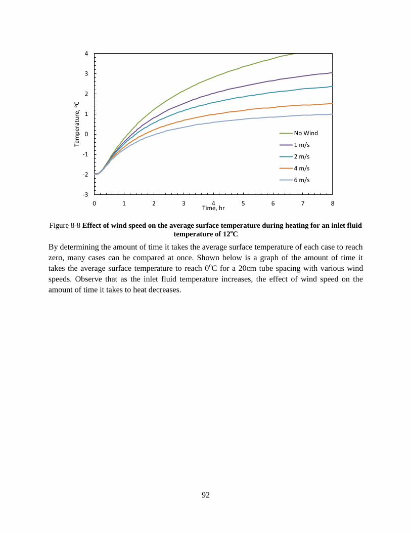
92
Figure 8-8 Effect of wind speed on the average surface temperature during heating for an inlet fluid
temperature of 12oC
By determining the amount of time it takes the average surface temperature of each case to reach
zero, many cases can be compared at once. Shown below is a graph of the amount of time it
takes the average surface temperature to reach 0oC for a 20cm tube spacing with various wind
speeds. Observe that as the inlet fluid temperature increases, the effect of wind speed on the
amount of time it takes to heat decreases.
-3
-2
-1
0
1
2
3
4
0 1 2 3 4 5 6 7 8
Tem
per
atu
re,
oC
Time, hr
No Wind
1 m/s
2 m/s
4 m/s
6 m/s

93
Figure 8-9 Effect of wind speed on deck surface heating
The effect of circulation tube spacing is also investigated, as this is one of the primary design
factors. The heating durations required to reach 0°C average deck surface temperature are shown
in Figure 8-10 for different tube spacings. In this case, the concrete cover thickness above the
tubes is 5.7 cm and ambient air temperature is -2°C. Tube spacing of 15 cm results in 19-30%
reduction in heating time to reach 0°C average deck surface temperature in comparison to 20 cm
tube spacing for different inlet fluid temperatures. Similarly, 25 cm and 30 cm tube spacings
result in 20-38% and 41-85% increase in heating periods, respectively, in comparison to 20 cm
tube spacing. As shown, it is possible to heat the bridge deck with these tube spacings within
reasonably short time periods for the range of considered inlet fluid temperatures.
0.00
1.00
2.00
3.00
4.00
5.00
6.00
7.00
8.00
5.0 10.0 15.0 20.0
Tim
e, h
ou
rs
Fluid Temperature, oC
0 m/s
1 m/s
2 m/s
4 m/s
6 m/s
Wind Speed

94
Figure 8-10 Effect of tube spacing on the amount of time it takes to heat the surface for no wind and
an ambient temperature of -2oC
Thickness of the concrete overlay above the circulation tube can vary due to a variety of project
considerations. Therefore our analyses also included cases where the thickness of the concrete
cover was varied from the base case value of 5.7 cm. The results for the heating time to reach
0°C average deck surface temperature are shown in Figure 8-11 for different concrete cover
thicknesses. It appears that every centimeter of cover thickness adds about 10-20 minutes to the
bridge deck heating for the above metric. Within this given range, thickness of the concrete
cover has a smaller effect on heating time for closer spaced tubes in comparison to more
distantly spaced ones.
0
1
2
3
4
5
5.0 10.0 15.0 20.0
Tim
e, h
ou
rs
Fluid Temperature, oC
30
25
20
15
Tube Spacing (cm)

95
Figure 8-11 Effect of concrete thickness above tube on the amount of time it takes to heat the
surface for a 20cm tube spacing with no wind
The results for the effect of the fluid flow rate on deck heating are presented in Figure 8-12.
Several analyses were performed for 6, 8, 15 and 20 L/min flow rates in comparison to the 11.4
L/min in the base case. The effect of flow rate is relatively minor and slower flow rates result in
longer times to heat the bridge deck. A flow rate of 6 L/min results in a 13% increase in heating
time whereas 20 L/min results in a 6% decrease in heating time compared to 11.4 L/min flow
rate.
Figure 8-12 Effect of fluid flow rate on the amount of time it takes to heat the deck surface with
20cm tube spacing, -2oC ambient temperature, and no wind
0
1
2
3
4
5
5.0 10.0 15.0 20.0
Tim
e, h
ou
rs
Fluid Temperature, oC
3.7 cm (1.5in) to Tube Depth
5.7 cm (2.25in) to Tube Depth
7.7 cm (3.0in) to Tube Depth
9.7 cm (3.75in) to Tube Depth
1.00
1.10
1.20
1.30
1.40
0.0 5.0 10.0 15.0 20.0 25.0
Tim
e, h
ou
rs
Flow Rate, L/min
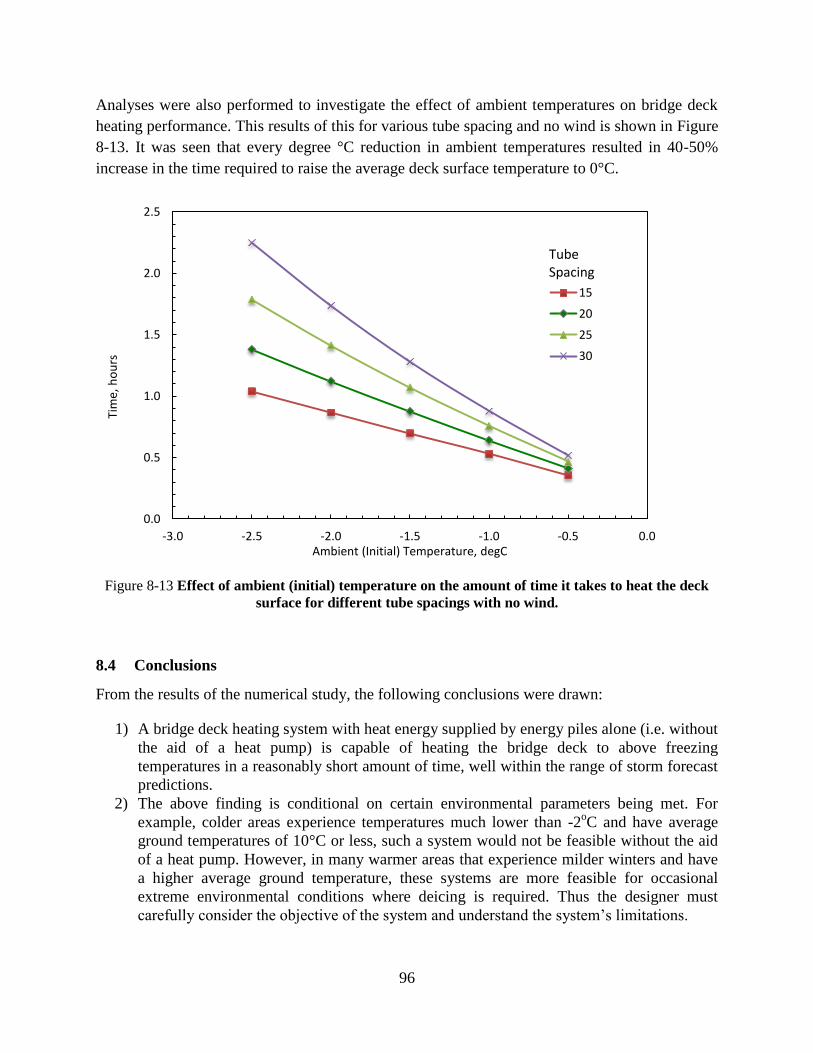
96
Analyses were also performed to investigate the effect of ambient temperatures on bridge deck
heating performance. This results of this for various tube spacing and no wind is shown in Figure
8-13. It was seen that every degree °C reduction in ambient temperatures resulted in 40-50%
increase in the time required to raise the average deck surface temperature to 0°C.
Figure 8-13 Effect of ambient (initial) temperature on the amount of time it takes to heat the deck
surface for different tube spacings with no wind.
8.4 Conclusions
From the results of the numerical study, the following conclusions were drawn:
1) A bridge deck heating system with heat energy supplied by energy piles alone (i.e. without
the aid of a heat pump) is capable of heating the bridge deck to above freezing
temperatures in a reasonably short amount of time, well within the range of storm forecast
predictions.
2) The above finding is conditional on certain environmental parameters being met. For
example, colder areas experience temperatures much lower than -2oC and have average
ground temperatures of 10°C or less, such a system would not be feasible without the aid
of a heat pump. However, in many warmer areas that experience milder winters and have
a higher average ground temperature, these systems are more feasible for occasional
extreme environmental conditions where deicing is required. Thus the designer must
carefully consider the objective of the system and understand the system’s limitations.
0.0
0.5
1.0
1.5
2.0
2.5
-3.0 -2.5 -2.0 -1.5 -1.0 -0.5 0.0
Tim
e, h
ou
rs
Ambient (Initial) Temperature, degC
15
20
25
30
Tube Spacing

97
3) The major limitation due to the coupling of higher heating demand and colder ground
temperatures at colder environments can be overcome by collecting heat from the bridge
deck slab in the summer and injecting into the ground to be reclaimed in the winter when
needed. Thermal storage will result in higher circulation fluid temperatures in the winter,
which can reduce required heating durations as shown in the presented analyses.
4) Certain design factors such as closer spacing and less concrete cover can aid in increasing
the efficiency of a system by decreasing the amount of time it takes the deck to heat.
Increasing the fluid flow rate can also increase the efficiency of a system but its effects are
not as significant.
9. Cost analysis
9.1 Introduction to life cycle analysis (LCA)
In order to compare the feasibility of the ground-coupled bridge deck deicing system with the
conventional deicing systems, a life cycle analysis (LCA) framework was developed for the
deicing salt. LCA is a quantitative method, which aims to assess environmental and social
impacts through the whole product life cycle. According to International Organization for
Standardization (ISO 14040; ISO 14044, 2006), LCA is a "compilation and evaluation of the
inputs, outputs and the potential environmental impacts of a product system throughout its life
cycle." The Society of Environmental Toxicology and Chemistry (SETAC) also defined LCA as
“a process to evaluate the environmental burdens associated with a product, process, or activity
by identifying and quantifying energy and materials used and wastes released to the
environment; to assess the impact of those energy and materials used and releases to the
environment; and to identify and evaluate opportunities to affect environmental improvements.”
9.2 Steps of a LCA
LCA consists of four steps: (1) Goal and Scope Definition, (2) Inventory Analysis, (3) Impact
Assessment, and (4) Interpretation (Figure 9-1). Below is a description these steps in the deicing
salt LCA framework

98
Figure 9-1 LCA Steps according to ISO 14040
1) Goal and Scope Definition:
In this step, the scope and the boundary of the LCA is defined as well as the functional unit. The
type of methods, impact categories, and set of data that needs to be collected are also identified.
System boundary and functional unit definition are important elements of this component.
Functional unit is a description of a product or system to be assessed. The functional unit aids in
comparing the results of a LCA of a product with a similar product. The functional unit is
defined based on the needs of the assessment. For the deicing salt, the functional unit can be
defined as the entire life cycle of the product from the raw material extraction to the disposal to
the landfill. System boundary defines the scope of the assessment. The system boundary
indicates what products and life stages are considered for the LCA.
2) Life Cycle Inventory (LCI) Analysis:
The life cycle inventory analysis is the most critical step in LCA. In this step, the inputs
including energy and resources, and the outputs including the emissions to atmosphere, water,
and soil are quantified. The inputs and outputs are then combined in the process flow chart and
related to the functional basis (Bayer and Gentry, 2010). At this stage an inventory of all the
inputs and outputs to and from the production system is prepared. As an example, the inputs may
include electricity consumption and the outputs may include CO2. If the LCI results are
consistent and accurate, the products and processes can be compared and evaluated enabling
decision makers to make more environmentally friendly decisions.
According to a LCA Guideline developed for AIA, databases and LCA-based tools are critical in
providing accurate and reliable results (Bayer and Gentry, 2010). In the next section, the LCA-
based tools are highlighted.

99
3) Life Cycle Impact Assessment:
The life cycle impact assessment translates the result of LCI analysis into impacts on
environment and human health. The effects are categorized in various impact categories in order
for the users to gain a better understanding of the impacts. For example, the quantified emission
of CO2 is translated to its impact on ozone depletion layer. Furthermore, a single value result can
be obtained by applying weights to the LCI result. In this case, only one single value is reported
rather than multiple impact categories.
4) Interpretation:
In order to report the LCA result in the most informative way, the results are interpreted. The
aim of the interpretation step is to help decision makers to easily compare different scenarios;
and ultimately, make environmentally friendly decisions.
9.3 The life cycle of deicing salt (Calcium Chloride)
Figure 9-2 presents the system boundary of the life cycle of chemical deicing salts. It begins
(cradle) with raw material extraction, preparation, and treatment. From there, it is stored and
transported as it moves to the manufacturing process. After manufacturing, it is stored and
transported again before being spread on a deck, where it accomplishes its deicing purpose.
Afterwards, the remaining salt and byproducts are ideally collected and stored/transported on
their way to ultimate disposal in the landfill. However, this is almost never the case and the salt
usually ends up leaching into the environment. But that is outside of the boundaries of the system
of what can be considered. Thus, a cradle-to-gate approach is suggested to consider the life cycle
impacts of deicing salt. The ‘gate’ refers to the delivery of the product (the salt) to the user (the
bridge).

100
Figure 9-2 System boundary of the life cycle of deicing salt
9.4 Cradle-to-Gate life cycle assessment of deicing salt (Calcium Chloride CaCl2)
This section briefly describes a cradle-to-gate approach that could be implemented for the
assessment of deicing salt. The table below gives an overview of the product including its
description, which is the type of CaCl2 being considered, the project boundaries, the functional
unit, and the source of data for the analysis (project libraries).
Table 9-1 Product overview for a LCA of CaCl2
Product
Name
Description Project
Boundaries
Functional Unit Project Libraries
Calcium
Chloride
CaCl2, at regional
storage
Cradle-to-
Gate
1 kg Ecoinvent System
Processes
A proper analysis would include the environmental impacts from the raw materials used to
produce CaCl2, examples of which are given in the table below. Note that the amount represents
the amount of raw material required per functional unit (1kg) of CaCl2.

101
Table 9-2 Raw materials required for CaCl2 production and processing
Substance Amount (m2)
Transformation, from arable 4.75e-7
Transformation, from arable, non-irrigated 0.000115
Transformation, from arable, non-irrigated, fallow 1.08e-7
Transformation, from dump site, inert material landfill 1.06e-5
Transformation, from dump site, residual material landfill 4.35e-6
Transformation, from dump site, sanitary landfill 7.59e-8
Transformation, from dump site, slag compartment 3.08e-8
Transformation, from forest 4.85e-5
Transformation, from forest, extensive 0.000529
Transformation, from forest, intensive, clear-cutting 3.39e-7
Transformation, from industrial area 4.42e-7
Transformation, from industrial area, benthos 6.3e-10
Transformation, from industrial area, built up 3.14e-9
Transformation, from industrial area, vegetation 5.36e-9
Transformation, from mineral extraction site 1.48e-5
Transformation, from pasture and meadow 2.66e-5
Transformation, from pasture and meadow, intensive 9.36e-8
Transformation, from sea and ocean 1.46e-5
Transformation, from shrub land, sclerophyllous 1.67e-5
Transformation, from tropical rain forest 3.39e-7
Transformation, from unknown 0.000106
Transformation, to arable 6.11e-6
Transformation, to arable, non-irrigated 0.000115
Transformation, to arable, non-irrigated, fallow 2.29e-7
Transformation, to dump site 1.62e-5
Transformation, to dump site, benthos 1.44e-5
Transformation, to dump site, inert material landfill 1.06e-5
Transformation, to dump site, residual material landfill 4.35e-6
In addition there will be emissions to the air, water, and soil, examples of which are given below.
Again, note that the emissions represent the amount of emission of a given substance per
functional unit (1kg) of CaCl2.

102
Table 9-3 Emissions to air, water, and soil from CaCl2 production and transportation processes
Substance Emission Amount (kg)
1-Butanol Air 8.15E-14
1-Pentanol Air 3.47E-13
1-Pentene Air 2.62E-13
1-Propanol Air 8.14E-12
1,4-Butanediol Air 2.00E-11
2-Aminopropanol Air 1.08E-14
2-Butene, 2-methyl Air 5.81E-17
2-Methyl, 1-propanol Air 6.14E-13
2-Nitrobenzoic acid Air 1.55E-14
2-Propanol Air 3.73E-07
Acenaphthene Air 4.77E-13
Acetaldehyde Air 3.39E-07
Acetic acid Air 3.56E-07
Acetone Air 5.17E-07
Acetonitrile Air 3.68E-10
Acrolein Air 1.09E-10
Acrylic acid Air 9.64E-10
Aldehydes, unspecified Air 4.71E-09
Aluminum Air 0.000119
Ammonia Air 0.00132
Ammonium carbonate Air 1.00E-10
Aniline Air 1.47E-12
Anthranilic acid Air 1.13E-14
Antimony Air 4.29E-08
Arsenic Air 3.99E-07
Arsine Air 1.12E-14
Barium Air 7.79E-07
Benzal chloride Air 5.36E-17
Aclonifen Soil 1.26E-10
Aldrin Soil 2.48E-11
Aluminum Soil 4.99E-06
Antimony Soil 2.92E-12
Arsenic Soil 1.10E-09
Atrazine Soil 6.50E-12
Barium Soil 4.85E-07
Benomyl Soil 7.87E-13
Bentazone Soil 6.45E-11
Boron Soil 2.32E-08
Cadmium Soil 8.61E-10

103
Substance Emission Amount (kg)
Calcium Soil 1.89E-05
Carbetamide Soil 3.21E-11
Carbofuran Soil 4.32E-10
Carbon Soil 4.85E-05
Chloride Soil 5.59E-05
Chlorothalonil Soil 9.17E-09
Chromium Soil 2.27E-08
Chromium VI Soil 7.62E-08
Cobalt Soil 2.22E-09
Copper Soil 1.30E-07
Cypermethrin Soil 6.19E-11
Feniclonil Soil 3.65E-10
Fluoride Soil 1.00E-07
Glyphosate Soil 3.18E-08
Iron Soil 9.30E-05
Lead Soil 2.34E-08
Linuron Soil 9.79E-10
1-Butanol Water 6.27E-09
1-Pentanol Water 8.33E-13
1-Pentene Water 6.29E-13
1-Propanol Water 1.22E-12
1,4-Butanediol Water 8.00E-12
2-Aminopropanol Water 2.68E-14
2-Methyl, 1-propanol Water 1.47E-12
2-Methyl, 2-butene Water 1.40E-16
2-Propanol Water 1.38E-13
4-Methyl, 2-pentanone Water 3.18E-13
Acenaphthene Water 1.26E-11
Acenaphthylene Water 7.87E-13
Acetaldehyde Water 1.15E-08
Acetic acid Water 3.00E-08
Acetone Water 8.66E-12
Acetonitrile Water 7.17E-14
Acetyl chloride Water 6.54E-13
Acidity, unspecified Water 9.07E-09
Acrylate, ion Water 2.28E-09
Aluminum Water 0.00115
Aluminum, ion Water 4.21E-05
Aniline Water 3.54E-12
Antimony Water 1.45E-06

104
Substance Emission Amount (kg)
AOX, Adsorbable Organic Halogen
as Cl Water 8.11E-09
Arsenic, ion Water 4.41E-06
Barite Water 8.98E-06
Barium Water 1.64E-05
Benzene Water 5.10E-07
10. List of references
Abdelaziz SL, Olgun CG, Martin II JR (2011) Design and Operational Considerations of
Geothermal Energy Piles, Proceedings of Geo-Frontiers 2011, March 13-16, 2011,
Dallas, Texas.
Abdelaziz, S.L., (2013). Deep Energy Foundations: Geotechnical Challenges and Design
Considerations. PhD Thesis, Virginia Polytechnic Institute and State University,
Blacksburg, VA, 347 pp.
Adam, D. and Markiewicz, R. (2009). “Energy from Earth-Coupled Structures, Foundations,
Tunnels and Sewers.” Géotechnique. Vol. 59, No. 3, pp. 229–236.
American Association of State Highway and Transportation Officials (AASHTO). (2005).
“Grand Challenges: A Strategic Plan for Bridge Engineering.” AASHTO Subcommittee
on Bridges and Structures, June 2005.
American Association of State Highway and Transportation Officials (AASHTO). (2008).
“Bridging the Gap: Restoring and Rebuilding the Nation’s Bridges.” AASHTO
Subcommittee on Bridges and Structures, July 2008.
American Association of State Highway and Transportation Officials (AASHTO) (2012).
AASHTO LRFD Bridge Design Specifications, Customary U.S. Units, American
Association of State Highway and Transportation Officials (AASHTO), S.l.
American Concrete Institute (ACI) Committee 318. (2011). Building code requirements for
structural concrete (ACI 318-11) and commentary, American Concrete Institute,
Farmington Hills, MI.
American Society of Heating Refrigerating and Air-Conditioning Engineers (ASHRAE) (2011).
2011 ASHRAE Handbook – Heating, Ventilating, and Air-Conditioning Applications (SI
Edition). Atlanta, GA. American Society of Heating, Refrigerating and Air-Conditioning
Engineers, Inc.
Amis T, Bourne-Webb PJ, Davidson C, Amatya B, Soga K. The effects of heating and cooling
energy piles under working load at Lambeth College. UK. Proceedings 2008.
Baboian, R. (1992). “Synergistic Effects of Acid Deposition and Road Salts on Corrosion.”
Corrosion Forms and Control for Infrastructure, ASTM STP 1137, pp. 17-29.
Barnard, A.C.L., Hunt, W.A., Timlake, W.P. and Varley E., 1966. A theory of fluid flow in

105
compliant tubes. Biophysical Journal 6, 717–724.
Barrett, M.L., and Pigman, J.G. (2001). “Evaluation of Bridge Deck Anti-Icing System.”
Kentucky Transportation Center, Kentucky Highway Investigative Task No. 36.
Basu, P., Loukidis, D., Prezzi, M., and Salgado, R. (2011). Analysis of shaft resistance of jacked
piles in sands. International Journal for Numerical and Analytical Methods in
Geomechanics, 35(2011), pp. 1605–1635.
Bayer, C., and Gentry, R. (2010), "AIA Guide to Building Life Cycle Assessment in Practice",
Prepared for American Institute of Architects, Washington, Dc.
Bhattacharya M.C. An explicit conditionally stable finite difference equation for heat conduction
problems, International Journal for Numerical Methods in Engineering, 1985, 21: 239-
265.
Bieganousky, W. A. and Marcason III, W. E. (1976). “Uniform placement of sand.” Journal of
Geotechnical and Geoenvironmental Engineering, 102(ASCE# 11985).Boënnec, O.
(2009). “Piling on the energy”, Geodrilling International, March 2009, pp. 25-28.
Boënnec O. Piling on the energy, Geodrilling International, 2009; 25-28.
Bourne-Webb P.J., Amatya B., Soga K., Amis T., Davidson C., and Payne P. (2009). “Energy
Pile test at Lambert College, London: Geotechnical and Thermodynamic Aspects of Pile
Response to Heat Cycles.” Geotechnique, Vol. 59, No. 3, pp. 237-248.
Brandl, H. (2006). “Energy Foundations and Other Thermo-Active Ground Structures.”
Geotechnique. Vol. 56, No. 2, pp. 81-122.
Cady, P.D., and Weyers, R.E. (1983). “Chloride Penetration and the Deterioration of
Concrete Bridge Decks.” Cement, Concrete & Aggregate, Vol. 5, No. 2, pp. 81-87.
Carslaw HS, Jaeger JC. Heat Conduction in Solids. Claremore Press: Oxford; 1947.
Churchill, S.W., 1997. Friction factor equations spans all fluid-flow regimes, Chemical
Engineering 84, 91–92.
Courant R, Friedrichs K, Lewy H. On the partial difference equ.ations of mathematical physics.
IBM Journal 1967; 11: 215-234.
Cresswell, A., Barton, M. E., and Brown, R. (1999). Determining the maximum density of sands
by pluviation. ASTM geotechnical testing journal, 22(4), 324–328. Retrieved from
http://cat.inist.fr/?aModele=afficheN&cpsidt=1203284
Edwards D.K, Denny V.E, Mills A.F. Transfer process, Hamisphere Publishing Crop, New
York, 1979.
EGEC (2007) “Geothermal Snow Melting and De-Icing.” European Geothermal Energy Council,
Brussels, September 2007.
Eskilson P. Thermal analysis of heat extraction boreholes. Ph.D. Thesis, University of Lund,
Department of mathematical Physics: Lund: Sweden; 1987.
Eskilson P, Claesson J, Simulation model for thermally interacting heat extraction boreholes.

106
Numerical Heat Transfer 1988, 13: 149–165.
Fasullo, E.J. (1992). “Infrastructure: The Battlefield of Corrosion.” Corrosion Forms and Control
for Infrastructure, ASTM STP 1137, pp. 1-16.
Federal Highway Administration (FHWA) (2008). “Status of the Nation’s Highways, Bridges,
and Transit: Conditions & Performance” Report to Congress, U.S. Department of
Transportation Federal Highway Administration, Federal Transit Administration,
Washington D.C., 622 p.
Federal Highway Administration, (FHWA, 2010), “Drilled shafts: construction procedures and
LRFD design methods”, U.S. Department of Transportation.
Gao J., Zhang X., Liu J., Li K., Yang J. (2008a). Numerical and experimental assessment of
thermal performance of vertical energy piles: an application, Applied Energy 85; 901-
910.
Gao J., Zhang X., Liu J., Li K., Yang J. (2008b). Thermal performance and ground temperature
of vertical pile-foundation heat exchangers: a case study, Applied Thermal Engineering
28; 2295-2304.
Ghasemi-Fare, O. and Basu P. (2013a), An annular-cylinder source model for heat transfer
through energy piles. Compendium of Papers - 92nd Transportation Research Board
Annual Meeting, Washington D.C.
Ghasemi-Fare, O. and Basu P., (2013b). A practical heat transfer model for geothermal piles.
Energy and Buildings 66:470-479.
Ghasemi-Fare, O., Basu, P., and Banerjee, S. (2014) Reliability-Based Assessment of
Sustainable Heat Exchange through Pile Foundations. Geo-Congress 2014 Technical
Papers: pp. 3323-3332. doi: 10.1061/9780784413272.323
Ghasemi-Fare, O. and Basu, P. (2015) Thermal Operation of Geothermal Piles Installed in
Sand—A Comparative Assessment Using Numerical and Physical Models. IFCEE 2015:
pp. 1721-1730. doi: 10.1061/9780784479087.156
Ghasemi-Fare, O. (2015). Geothermal energy harvesting through pile foundation – analysis-
based prediction and performance assessment, Ph.D. dissertation, The Pennsylvania State
University, U.S.A.
Gnielinski V. New equations for heat and mass transfer in turbulent pipe and channel flow,
International Journal of Chemical Engineering, 1976; 16: 359–368.
Granata, R.D., and Hartt, W.H. (2009). “Integrity of Infrastructure Materials and Structures.”
FHWA-HRT-09-044, Federal Highway Administration, Washington, D.C.
Hamada Y, Saitoh H, Nakamura M, Kubota H, Ochifuji K. (2007). Field performance of an
energy pile system for space heating. Energy and Building; 39: 517-524, DOI:
10.1016/j.enbuild.2006.09.006.
Hoppe E.J., (2000). “Evaluation of Virginia's First Heated Deck Bridge.” Virginia
Transportation Research Council, Report No. VTRC 01-R8, December 2000.

107
Ingersoll LR, Zobel OJ, Ingersoll AC. Heat conduction with engineering geological and other
applications, second edition. McGraw-Hill; 1954.
Iskander, M. (2010). Behavior of pipe piles in sand. (W. Wu and R. I. Borja, eds.), Springer.
ISO 14040 (2006). "Environmental management - Life cycle assessment - Principles and
framework." International Organization for Standardization (ISO), Geneve, Switzerland.
Jalaluddin E, Miyara A, Tsubaki K, Inoue S, Yoshida K. (2011). Experimental study of several
types of ground heat exchanger using a steel pile foundation. Renewable Energy; 36:
764–771, DOI: 10.1016/j.renene.2010.08.011.
Javed S., Fahlen P. (2011). Thermal response testing of a multiple borehole ground heat
exchanger. International Journal of Low-Carbon Technologies, 6; 141-148.
Johnson, P.M., Couture, A., and Nicolet, R. (2007). “Report of the Commission of Inquiry into
the Collapse of a Portion of the de la Concrete Overpass.” Quebec, Government of
Quebec, ISBN 978-2-550-50961-5, October 2007, 198 p.
Kavanaugh, S.P., Xie, L. and Martin, C., 2001. Investigation of methods for determining soil and
rock formation from short term field tests. ASHRAE1118-TRP, American Society of
Heating, Refrigerating and Air-Conditioning Engineers, Inc., 77 pp.
Koch, G.H., Brongers, P.H., Thompson, N.G., Virmani, Y.P, and Payer, J.H. (2002). “Corrosion
Costs and Prevention Strategies in the United States.” Report No. FHWA-RD-01/156,
Federal Highway Administration, Washington, D.C., 2002.
Kraft, L. (1991), “Performance of axially loaded pipe piles in sand”, Journal of Geotechnical and
Geoenvironmental Engineering, Vol 117 (2), pp. 272-296.
Kramer C.A. (2013). “An experimental investigation on performance of a model geothermal pile
in sand”. M.S. dissertation, The Pennsylvania State University.
Kramer, A. C. and Basu, P. (2014a). Performance of a model geothermal pile in sand. Physical
Modelling in Geotechnics – Proceedings of the 8th International Conference on Physical
Modelling in Geotechnics (ICPMG) 2014, v 2, pp. 771-777, Perth, Australia, January 14-
17.
Kramer, A. C. and Basu, P. (2014b). Experimental characterization of energy output from a
model geothermal pile. Proceedings of Geocongress 2014, ASCE, Atlanta, Georgia,
February 23-26.
Kramer C.A, Ghasemi-Fare O, Basu P. (2014) P Laboratory thermal performance tests on a
model heat exchanger pile in sand, Journal of Geotechnical and Geological Engineering
Special Issue on “Thermo-mechanical Response of Soils, Rocks, and Energy
Geostructures”.
Kusuda, T., and Achenbach, P.R. (1965) “Earth temperature and thermal diffusivity at selected
stations in the United States.” ASHRAE Transactions, Vol. 71, Part 1, pp. 61-74.
Laloui, L., Nuth, M. and Vulliet, L. (2006). “Experimental and numerical investigations of the
behavior of a heat exchanger pile”, International Journal for Numerical and Analytical

108
Methods in Geomechanics, Vol. 30, pp. 763–781.
Lamarche L, Kajl S, Beauchamp B. (2010). A review of methods to evaluate borehole thermal
resistances in geothermal heat-pump systems. Geothermics; 39: 187-200, DOI:
10.1016/j.geothermics.2010.03.003.
Lings, M. L., and Dietz, M. S. (2005). “The peak strength of sand-steel interfaces and the role of
dilation.” Soils and Foundations, 45(6), pp. 1–14.
Liu, Y. (1996). “Modeling the Time-to-Corrosion Cracking of the Cover Concrete in Chloride
Contaminated Reinforced Concrete Structures.” Ph.D. Dissertation, Virginia Polytechnic
Institute and State University, Blacksburg, VA, December 1996, 117 p.
Liu, X., Rees, S. J., and Spitler, J. D. (2003). "Simulation of a Geothermal Bridge Deck Anti-
Icing System and Experimental Validation." 82nd Annual Meeting of the Transportation
Research BoardWashington, DC.
Liu, X., Rees, S. J., and Spitler, J. D. (2007a). "Modeling snow melting on heated pavement
surfaces. Part I: Model development." Applied Thermal Engineering, 27(5-6), 1115-
1124.
Liu, X., Rees, S. J., and Spitler, J. D. (2007b). "Modeling snow melting on heated pavement
surfaces. Part II: Experimental validation." Applied Thermal Engineering, 27(5-6), 1125-
1131.
Liu, X., and Spitler, J. D. (2004). "A Simulation Tool for the Hydronic Bridge Snow Melting
System." 12th International Road Weather ConferenceBingen, Germany.
Man Y., Yang H., Diao N., Liu J., Fang Z., (2010). A new model and analytical solutions for
borehole and pile ground heat exchangers, International Journal of Heat and Mass
Transfer; 53: 2593-2601.
Marcotte, D., Pasquier, P., 2008. On the estimation of thermal resistance in borehole thermal
conductivity test. Renewable Energy 33, 2407–2415.
McCartney JS, LaHaise D, LaHaise T, Rosenberg JE. (2010). Application of Geoexchange
Experience to Geothermal Foundations. The art of foundation engineering practice.
Geotechnical Special Publication No. 198, Hussein, M. H., Anderson, J. B. and Camp,
W. M. (eds.); 411-421.
McCartney JS, LaHaise D, LaHaise T, Rosenberg JE. Application of Geoexchange Experience to
Geothermal Foundations. The art of foundation engineering practice. Geotechnical
Special Publication No. 198, Hussein, M. H., Anderson, J. B. and Camp, W. M. (eds.)
2010; 411-421.
Minsk, D. (1999). “Heated Bridge Technology.” Final Report, Report No. FHWA-RD-99/158,
Federal Highway Administration, Washington, D.C., 1999.
Naito, C., Sause, R., Hodgson, I., Pessiki, S., and Macioce, T. (2010). “Forensic Examination of
a Non-Composite Adjacent Precast Prestressed Concrete Box Beam Bridge.” ASCE
Journal of Bridge Engineering, Vol. 15, No. 4, pp. 408-418.

109
Nam Y, Ooka R, Hwang S. (2008). Development of a numerical model to predict heat exchange
rates for a ground-source heat pump system. Energy and Buildings; 40: 2133-2140, DOI:
10.1016/j.enbuild.2008.06.004.
National Instruments (2011). LabVIEW. Vers. 2011. National Instruments. Computer software.
Nydahl, J., Pell, K., Lee, R., and J. Sackos, J. (1984). “Evaluation of an Earth Heated Bridge
Deck.” USDOT Contract No. DTFH61-80-C-00053, University of Wyoming, Laramie.
Olgun, C.G., Martin, J.R., Bowers G.A. (2012) “Energy Piles: Using Building Foundations as
Heat Exchangers”, Geo-Strata, Professional Magazine of the Geo-Institute, American
Society of Civil Engineers, March/April 2012.
Olgun, C.G., Sezen A., Martin, J.R., Abdelaziz, S.L. (2010). “Renewable Energy Applications in
Geotechnical Engineering.” ZM13, 13th Turkish National Conference on Soil Mechanics
and Geotechnical Engineering, Invited Keynote Lecture, September 30-October 1 2010,
Istanbul Turkey (In Turkish).
Ooka, R., Sekine, K., Mutsumi, Y., Yoshiro, S. SuckHo, H. (2007). “Development of a Ground
Source Heat Pump System with Ground Heat Exchanger Utilizing the Cast-in Place
Concrete Pile Foundations of a Building.” EcoStock 2007. 8 pp.
Ozudogru, T.Y., Olgun, C.G. and Senol, A., (2014a). 3D numerical modeling of vertical
geothermal heat exchangers. Geothermics 51, 312–324.
Ozudogru, T., Ghasemi-Fare, O., Olgun, G. and Basu, P. (2014b). Numerical modeling of
vertical geothermal heat exchangers using finite difference and finite element techniques.
Geotechnical and Geological Engineering; 33; pp. 291-306; Special Issue on – Thermo-
mechanical Response of Soils, Rocks, and Energy Geostructures; Springer; DOI
10.1007/s10706-014-9822-z
Parkin, A. K. and Lunne, T. (1982). “Boundary effects in the laboratory calibration of a cone
penetration for sand,” Proceeding of the Second European Symposium on Penetration
Testing, Netherlands National Society for Soil Mechanics & Foundation Engineering
(NNSSMFE), pp. 761–768.
Petukhov B.S, Heat Transfer and Friction in Turbulent Pipe Flow with Variable Physical
Properties. Advances in Heat Transfer, J. P. Hartnett and T. F. Irvine, J,R.(EDS.), 6: 503-
564, Academic Press, New York , 1970.
Plazak, D.J. (2008). “Strategic Highway Research in the United States.” November 2008,
Transportation Research Board, The National Academies, 33 p.
Poupard, O., Ait-Mokhtar, A., and Dumargue, P. (2004) “Corrosion by Chlorides in Reinforced
Concrete: Determination of Chloride Concentration Threshold by Impedance
Spectroscopy.” Cement and Concrete Research, Vol. 34, No. 6, pp. 991-1000.
Presetschnik, A., and Huber, H. (2005). "Analysis of a Ground Coupled Heat Pump Heating and
Cooling System for a Multi-story Office Building.” Proceedings of the 8th International
Energy Agency, Heat Pump Conference 2005, pp. 4-8.

110
Rad, N. S. and Tumay, M. T. (1987). “Factors affecting sand specimen preparation by
raining.” ASTM Geotechnical Testing Journal, 10 (1).
Rees, S. J., Spitler, J. D., and Xiao, X. "Transient analysis of snow-melting system
performance." Proc., ASHRAE Transactions 2002, June 22, 2002 - June 26, 2002, Amer.
Soc. Heating, Ref. Air-Conditoning Eng. Inc., 406-423.
Roosevelt, D.S. (2004). “A Bridge Deck Anti-icing System in Virginia : Lessons Learned from a
Pilot Study.” Virginia Transportation Research Council, Report No. VTRC 04-R26, June
2004.
Rouissi K, Krarti M, McCartney JS. (2012). Analysis of thermo-active foundations with U-tube
heat exchangers. Journal of Solar Energy Engineering, ASME; 134: 021008-1 - 021008-
8.
Salgado, R. (2008). “Analysis and design of single piles” The Engineering of Foundations.
Chapter 13, pp. 547-550.
Salgado, R., Mitchell, J. K., and Jamiolkowski, M. (1998). “Calibration chamber size effects on
penetration resistance in sand,” J. Geotech. Geoenviron. Eng., Vol. 124, No. 9, pp. 878–
888.
Schnaid, F. and Houlsby, G. T. (1991). “An assessment of chamber size effects in the calibration
of in situ tests in sand,” Geotechnique, Vol. 41, No. 3, pp. 437–445.
Spitler, J.D., and Ramamoorthy, M. (2000). “Bridge Deck Deicing using Geothermal Heat
Pumps.” Proceedings of the Fourth International Heat Pumps in Cold Climates
Conference, Aylmer, Québec, August 17-18, 2000.
Strategic Highway Research Program 2 (SHRP2) (2006). “Accelerating Solutions for Highway
Safety, Renewal, Reliability, and Capacity.” 2006 Annual Report, Transportation
Research Board, The National Academies.
Suryatriyastuti ME, Mroueh H, Burlon S. (2012). Understanding the temperature-induced
mechanical behavior of energy pile foundations. Renewable and sustainable Energy
Reviews; 16: 3344-3354, DOI: 10.1016/j.rser.2012.02.062.
Tarnawski V.R., Momose T., and Leong W.H. (2011). Thermal conductivity of standard sands
II. Saturated conditions, International Journal of Thermophysics 32; pp. 984-1005.
Tuutti, K. (1982). “The Corrosion of Steel in Concrete.” Swedish Cement and Concrete Research
Institute, Stochkolm. 469 p.
Uesugi, M. and Kishida, H. (1986). “Influential factors of friction between steel and dry sands.”
Soils and Foundations, 26 (2), pp. 33–46.
Uesugi, M., Kishida, H., and Tsubakihara, Y. (1988). “Behavior of sand particle in sand-steel
friction.” Soils and Foundations, 28 (1), pp. 107–118.
Virmani, Y.P, Jones, W.R., and Jones, D.H. (1984). “Steel Corrosion in Concrete: pH at
Corrosion Sites.” Public Roads, Vol. 84, No. 3, pp. 96.
Virmani, Y.P., Clear K.C., Pasko, T.J. (1983). “Time-To-Corrosion of Reinforcing Steel in

111
Concrete: Vol.5 Calcium Nitrite Admixture or Epoxy-Coated Reinforcing Bars as
Corrosion Protection Systems.” Report No. FHWA-RD-83/012, Federal Highway
Administration, Washington, D.C., 1983.
Wang, K., Nelsen, D.E. and Nixon, W.A. (2006). “Damaging Effects of Deicing Chemicals on
Concrete Materials.” Cement & Concrete Composites, Vol. 28, pp. 173-188.
White, D.J., Sritharan, S., Suleiman, M.T., Mekkawy, M.M., and Chulter, S. (2005).
“Identification of the Best Practices for Design, Construction, and Repair of Bridge
Approach Sections.” Final Report, Iowa DOT TR-481, CTRE Report 02-118.
Witte, H.J.L., van Gelder, G.J., and Spitler, J.D., (2002). In situ measurement of ground thermal
conductivity: a Dutch perspective. ASHRAE Transactions 108 (Part 1), 263–272.
Yavusturk C. (1999). Modeling of vertical ground loop heat exchangers for ground source heat
pump systems. Ph.D. Thesis, Oklahoma State University, USA.
Yunovich, M., Thompson, N.G., and Virmani, Y.P. (2003). “Life Cycle Cost Analysis for
Reinforced Concrete Bridge Decks.” Paper No. 03309, Presented at CORROSION/03,
San Diego, CA.
Zemajtis, J. (1998). “Modeling the Time to Corrosion Initiation for Concretes with Mineral
Admixtures and/or Corrosion Inhibitors in Chloride-Laden Environments.” Ph.D.
Dissertation, Virginia Polytechnic Institute and State University, Blacksburg, VA,
January 1996, 140 p.
Zeng H.Z., Diao N.R., Fang Z.H. (2002). A finite line-source model for boreholes in geothermal
heat exchangers, Heat Transfer-Asian Research; 31(7): 558-567.