Master of Science Thesis

KTH School of Industrial Engineering and Management

Energy Technology EGI-2016-050 EKV1149

Division of Heat and Power Technology

SE-100 44 STOCKHOLM

A fatigue investigation in a Kaplan

hydropower station operated in

frequency regulating mode

Aron Tapper

-2-

Master of Science Thesis EGI 2016:050

EKV1149

A fatigue investigation in a Kaplan hydropower

station operated in frequency regulating mode

Aron Tapper

Approved

20160620

Examiner

Björn Laumert

Supervisor

Jens Fridh

Commissioner

Voith Hydro AB

Contact person

Tony Bjuhr

Abstract

Due to the increase of intermittent power in the Nordic grid the need for frequency regulation increases.

Hydropower has the ability to respond fast to frequency changes in the grid and is the power source

mainly used to regulate the frequency in the Nordic grid. There are different types of frequency regulation

and this thesis has focused on primary frequency regulation which purpose is to keep the frequency within

the range of ±0.1 Hz from the nominal frequency.

For a hydropower station operated in frequency regulating mode the amount of movements in the

regulating mechanism increases, especially if it is a Kaplan turbine since it can regulate both the guide

vanes and the runner blades. When the hydropower station changes the produced power there are large

servomotor forces applied to the regulating mechanism to open or close the wicket gate and the runner

blade. During frequency regulation these changes occurs frequently and the risk of fatigue failure

increases.

The resulting servomotor force in the wicket gate and the runner was calculated from measured data of

the servomotor pressure and the dimensions of the servomotors. The angles between the components in

the regulating mechanism were calculated knowing the angle of the guide vanes and the runner blades,

which was used for translating the servomotor force through the regulating mechanism. The stresses in

each component were calculated and the stress cycles were counted which was used to estimate the life

time of the components.

The larges stresses in the regulating mechanism were found in the runner links and the connecting pins in

the runner. In the wicket gate the largest stresses were calculated in the connecting pin between the

servomotor and the operating ring, however the stress amplitudes were small, thus fatigue calculations

were considered unnecessary. Both the link and connecting pin has an estimated life time which is larger

than the commonly used turbine life time of 40-50 years. Even though the life time of the components are

above the design criteria it could be improved by implementing a two measure filtering system develop by

Voith Hydro.

-3-

Sammanfattning

På grund av ökande intermittenta kraftkällor i det Nordiska elnätet ökar behovet av frekvensreglering.

Vattenkraft kan reagera snabbt när frekvensen ändras i elnätet och är den kraftkälla som huvudsakligen

används i det Nordiska elnätet för att reglera frekvensen. Det finns olika typer av frekvensreglering men

detta examensarbete har enbart fokuserat på primär frekvensreglering, vilket har som syfte att hålla

frekvensen inom spannet ±0.1 Hz från den nominella frekvensen.

Om ett vattenkraftverk börjar reglera frekvensen på elnätet så innebär det ökade rörelser i

reglermekanismen, speciellt om det är en Kaplanturbin eftersom att den kan reglera både led- och

löpskovlarna. När ett vattenkraftverk ändrar uteffekten innebär det att servomotorer kommer att applicera

stora krafter till reglermekanismen för att öppna eller stänga pådraget och löpskovlarna. Vid

frekvensreglering förekommer frekventa ändringar av uteffekten vilket innebär en ökad risk för

utmattningsbrott.

Kraften från servomotorn i ledkransen och löphjulet räknades ut från mätdata över trycket i

servomotorerna och genom att veta servomotorernas dimensioner. Genom att veta positionen på led- och

löpskovlar så kunde vinklarna mellan komponenterna i reglermekanismen bestämmas och med hjälp av

dessa kunde kraften från servomotorn överföras till komponenterna. Spänningarna i komponenterna

beräknades, spänningscyklerna räknades och sedan användes dessa till att uppskatta livstiden för varje

komponent.

De största spänningarna i reglermekanismen beräknades i länken och länktappen i löphjulet. I ledkransen

så var spänningarna störst i tappen mellan servomotorn och reglerringen, dock var spänningarna av

amplituder så att utmattningsberäkningar inte ansågs nödvändigt. Både länken och länktappen hade en

uppskattad livstid som var större än 40-50 år, vilket ofta används som den livstid en turbin minst ska klara

av. Även om de beräknade livstiderna är över den minsta livstiden för en turbin så kan livstiden ökas

ytterligare genom ett filtreringssystem utvecklat av Voith Hydro.

-4-

Acknowledgment

This thesis has been carried out together with KTH Royal Institute of Technology and Voith Hydro AB.

A special thanks to Voith for the opportunity to do my thesis work with them, it has been a great

experience and a valuable insight to the field of hydropower. I want to thank everyone at Voith that has

helped me throughout the thesis, a lot of people have helped me from the office in Kristinehamn and

Västerås as well as the office in Heidenheim and I’m very grateful for that. I also want to extend a special

thanks to KTH for a great master program and to the lecturers and staff that has helped me throughout

these two years. Thanks to Fortum Generation AB for letting me conduct the measurements in their

hydropower station Jössefors.

I want to thank my supervisor at Voith, Tony Bjuhr, and Björn Hellström for the great support given and

the time you put into the thesis. At KTH I want to thank my supervisor, Jens Fridh, and my examiner,

Björn Laumert, for the valuable input regarding the report and guidance given through the thesis.

-5-

Table of Contents

Abstract ........................................................................................................................................................................... 2

Sammanfattning ............................................................................................................................................................. 3

Acknowledgment ........................................................................................................................................................... 4

1 Introduction .......................................................................................................................................................... 7

1.1 Objectives ..................................................................................................................................................... 7

1.2 Delimitations ................................................................................................................................................ 7

1.3 Method .......................................................................................................................................................... 8

2 Background ........................................................................................................................................................... 9

2.1 Kaplan turbine ............................................................................................................................................. 9

2.1.1 The Governor ...................................................................................................................................10

2.2 Hydraulic power system ...........................................................................................................................12

2.2.1 Oil pressure system ..........................................................................................................................12

2.2.2 Servomotor .......................................................................................................................................12

2.3 Regulation mechanism .............................................................................................................................13

2.3.1 Guide vane regulation .....................................................................................................................13

2.3.2 Runner blade regulation ..................................................................................................................14

2.4 Frequency regulation ................................................................................................................................15

2.4.1 Primary frequency control ..............................................................................................................15

2.4.2 Secondary frequency control ..........................................................................................................16

2.4.3 Regulating power .............................................................................................................................16

2.5 Dead-band and filtering systems ............................................................................................................16

2.6 Jössefors hydropower station ..................................................................................................................17

3 Measurement on site ..........................................................................................................................................18

3.1 Preparations ...............................................................................................................................................18

3.2 Execution & data gathering .....................................................................................................................19

4 Calculation method ............................................................................................................................................20

4.1 Angles in the guide vane regulating mechanism ..................................................................................20

4.2 Angles in the runner blade regulating mechanism ...............................................................................23

4.3 Forces and stresses in the wicket gate ...................................................................................................24

4.3.1 The lever ............................................................................................................................................24

4.3.2 The link ..............................................................................................................................................26

4.3.3 The connecting pins ........................................................................................................................27

4.4 Forces and stresses in the runner ...........................................................................................................27

4.4.1 The lever ............................................................................................................................................27

4.4.2 The link ..............................................................................................................................................28

4.4.3 The crosshead ...................................................................................................................................29

-6-

4.4.4 The crosshead keys ..........................................................................................................................30

4.4.5 The connecting pins ........................................................................................................................30

4.5 Fatigue and life time calculations ............................................................................................................31

4.5.1 Rain-flow count ................................................................................................................................31

4.5.2 Palmgren-Miner rule ........................................................................................................................31

4.5.3 S-N curve ..........................................................................................................................................32

5 Results ..................................................................................................................................................................34

5.1 Data from the measurement ...................................................................................................................34

5.2 Provided data .............................................................................................................................................36

5.3 Forces in the wicket gate ..........................................................................................................................41

5.4 Forces in the runner .................................................................................................................................42

5.5 Stresses in the wicket gate ........................................................................................................................44

5.6 Stresses in the runner ...............................................................................................................................45

5.7 Life time evaluations .................................................................................................................................49

6 Discussion ...........................................................................................................................................................58

6.1 The results ..................................................................................................................................................58

6.1.1 Wicket gate ........................................................................................................................................58

6.1.2 Runner ...............................................................................................................................................58

6.2 Limitations of the investigation ..............................................................................................................59

7 Conclusions .........................................................................................................................................................61

Bibliography .................................................................................................................................................................62

-7-

1 Introduction

As more countries agree to decrease the emissions of greenhouse gases by increase the share of renewable

energies, hydropower might be an important part of the transition. Hydropower is a mature technology

with the ability to serve as base load as well as frequency regulation. Modern society relies on the

availability of electricity at all times hence it is important to have a reliable power source with the ability to

respond fast to sudden changes in the power grid.

Due to the increase of wind, solar and wave energy in the power system the power fluctuations is

expected to increase. With these fluctuations the need for regulating the frequency and regulating the

power shortage/abundance will increase. Hydropower is often used as regulating power reserve because it

can respond fast to a shortage or abundance of power in the grid. Hence the need for regulating

hydropower will increase.

Associated with regulating hydropower are load variations which increase the wear and tear in the

hydropower plant. This could lead to decreased lifetime of several mechanical parts and the hydropower

plant in whole. To estimate the decreased lifetime of the hydropower plant, if operated in frequency

regulating mode, it is important to understand which factors that are affecting and affected when

regulating the power output.

1.1 Objectives

The purpose of the thesis is to increase the understanding of frequency regulation and the impact it has on

the mechanical parts in a hydropower plant. This thesis can be divided into the following deliverables;

Investigate and identify the emergence or increase of stresses and fatigue in the hydraulic power

system when a hydropower plant is operated in frequency regulating mode. This investigation will

calculate the stresses in the mechanical parts of the regulating system and evaluate the effect that

frequency regulation has on the lifetime of the mechanical parts. The main focus of the

investigation will be on the regulating mechanism in the wicket gate and the runner, including the

links, link pins and levers that regulate the runner blades and guide vanes.

Set up equations and models for determining the forces and stresses that are associated with

frequency regulation.

Pressure measurements in a hydropower plant, in the hydraulic power system, during frequency

regulation. In the hydraulic power system it is the opening and closing pressure of the servomotor

in both the wicket gate and runner that will be measured. The measured servomotor pressures

will be used to calculate the stresses acting on the regulating system during frequency regulation.

The measured data will be evaluated in the models to make a risk assessment of the investigated

parts of the hydropower plant.

1.2 Delimitations

The focus of the investigation will be on the forces associated with load variation and how these forces

will affect the mechanical parts in the hydraulic power system which includes the oil pressure system and

servomotors. An investigation on how the bearings in the wicket gate and the runner are affected by

frequency regulation has already been carried out so the bearings will not be investigated in this thesis [1].

Further, this thesis will only focus on Kaplan turbines and one reason is that it is a common type of

turbine used in Sweden. The other reason is that the Kaplan turbine has adjustable runner blades and an

additional regulation mechanism which means more mechanical parts that could be subjected to wear and

tear.

-8-

The occurrence of cavitation, erosion and vortexes are some complex phenomenon that needs to be

considered while investigating parts that operate in water. Due to the complexity, none of the mechanical

parts operating in the water flow will be investigated.

It is assumed that the components have been mounted properly and that the materials meet the

specification of the manufacturer.

1.3 Method

To enhance understanding of frequency regulation, hydraulic dynamics and the critical parameters

associated with hydropower regulation a literature review will be carried out together with interviews. The

critical mechanical parts will be identified and explained why these parts need to be investigated further.

Simplified equations will be used to relate the forces caused by frequency regulation to the identified

critical parts. These equations will relate the resulting forces acting on the critical parts to the pressure

fluctuations in the hydraulic power system. When the forces have been calculated the stresses in the

identified components will be calculated and with stress concentration factors the local stress

concentrations will be calculated. This will be compiled in MATLAB to create a model which displays the

forces acting on the critical parts and the cyclic forces during frequency regulation.

In a hydropower plant, the pressure fluctuations in the servomotors will be measured along with the

angles of the guide vanes and runner blades while the plant is operated in frequency regulating mode.

These measurements will be inserted in the created MATLAB model which will display the resulting and

cyclic forces and stresses acting on the identified critical parameters. Knowing the number of cycles

during the expected lifetime, the magnitude of stresses and the manufacturing data of a certain part the

impact of frequency regulation will be assessed.

-9-

2 Background

2.1 Kaplan turbine

The Kaplan turbine is an axial type turbine. The water from the penstock is distributed by the spiral and

enters the runner chamber through the wicket gate. Between the wicket gate and the runner the water is

diverted from radial to axial flow. When the water has passed the runner it is discharged through the draft

tube. The placement of the generator depends of the layout of the Kaplan turbine, a common layout is the

vertical turbine which can be seen in figure 1. In such a layout the generator is placed above the turbine

which is connected to the turbine through the turbine-generator shaft [2].

Figure 1, shows a typical layout of a vertical Kaplan turbine [3].

The wicket gate consists of adjustable guide vanes which control the water flowing into the runner

chamber. The regulating mechanism of the wicket gates consists of a linkage, operating ring and

servomotor, which controls the angle of the guide vanes. The runner blades are regulated by a servomotor

through linkage as the guide vanes but in a different configuration. There are typically two types of

configuration of the servomotor regulating the runner blades, either constructed as a part of the turbine

shaft, as shown in figure 1, or as an extern part inside the runner hub [4].

The characteristic feature of a Kaplan turbine is the adjustable runner blades, which are fixed in a regular

propeller turbine. The advantage of adjustable compared to fixed blades is that the adjustable blades can

operate over a large range of different water flows and power outputs and still maintain a high efficiency.

-10-

Figure 2 shows the efficiency curve of a Kaplan turbine, together with the definition of the runner blade

angle. While the efficiency is measured as a function of the flow rate through the wicket gate, the runner

blade angle α1 is kept constant and so is the rotational speed of the turbine. The same procedure is carried

out with a new runner blade angle and is repeated until the total span of runner blade angles has been

covered. From the results a trend line can be drawn which combines the flow rate with the optimal runner

blade angle for a given rotational speed. The turbine governor is programed according to the measured

results and combines a certain guide vane angle with the optimum runner blade angle so that the turbine is

operated at the optimal efficiency [2].

Figure 2, shows the efficiency curve of a Kaplan turbine and the runner blade angle (α). Q is the flow rate through the wicket gate, n is the rotational speed and η is the turbine efficiency [2].

2.1.1 The Governor

The main function of the turbine governor, also known as a speed governor, is to keep the turbine and

generator at constant rotational speed or in reality to minimize the deviations in rotational speed and time

until the rotational speed has been restored. To understand the purpose of the governor it is important to

understand the forces behind the rotational speed of the turbine-generator set.

The relation between power (P [kW]), rotational speed (n [rpm]), torque (T [Nm]) and a constant k is

shown in equation (2.1).

𝑃 = 𝑘 ∗ 𝑇 ∗ 𝑛 (2.1)

Σ𝑇𝑖 = (𝑑𝜔

𝑑𝑡) ∗ 𝐽 (2.2)

Equation (2.2) it can be seen that the sum of the driving and the load torque (∑Ti [Nm]) is proportionate

with the rotational acceleration (dω/dt [rad/s2]) because the moment of inertia of the rotating mass (J

[kg*m2]) is constant. The load torque is the torque that is required to drive the generator while the driving

torque is the torque in the turbine shaft. If the torque required by the generator is deviating from the

driving torque then the rotating mass will either accelerate or decelerate. If the rotational mass is

decelerating, i.e. the loading torque is larger than the driving torque, equation (2.1) shows that the available

power needs to be increased to increase the driving torque hence keeping the rotational speed constant [4]

[5].

The maximum speed that the turbine can reach is called runaway speed, which occurs when the torque

required by the generator is zero. This will cause the turbine to accelerate until all available power is

converted to kinetic energy and losses [5].

-11-

Figure 3 shows a block diagram over the speed control loop. The difference in load and power results in a

certain speed which is compared to a reference speed and it is the governors purpose to adjust the

available power from the turbine so that the speed deviation is corrected [4].

Figure 3, shows the speed control loop in a turbine [4].

The turbine governor can be either a pure mechanical, mechanical-hydraulic, mechanical-electric or

electric-hydraulic. Figure 4 shows a basic configuration of a mechanical-hydraulic turbine governor, where

the flywheel is connected to the turbine shaft and to the sleeve of the pilot valve. If the turbine speed

increases, the flywheel will spin faster and pulls the connecting rod upwards, this causes the sleeve of the

pilot valve to move down. The pressurized oil can flow into the servomotor which will close the wicket

gate until the flywheel is slowed down and is returned to its original position.

Figure 4, shows a basic configuration of a mechanical speed governor [6].

The electric-hydraulic governor is a modern type of the governor described above. Instead of the flywheel

the turbine speed is measured through sensors on the turbine shaft and compared to a reference value. If

-12-

the turbine speed deviates from the reference a signal is sent to the servomotor which adjusts the wicket

gate until the deviation signal is corrected [6].

If the torque required from the generator is suddenly decreased while the wicket gate remains unchanged

then the rotational speed will increase which increase the wear of the turbine. It is important that the

governor can adjust the wicket gate fast enough to keep the rotational speed below the prescribed limit of

the turbine. Although, if the wicket gate is closed to fast the pressure will rise and this can cause surge in

the pipeline [4].

2.2 Hydraulic power system

The working principle of an hydraulic power system is to convert mechanical power to hydraulic power

through a pump, then transmit the hydraulic power through pipelines, the hydraulic power is controlled

by valves and a servomotor converts hydraulic power to mechanical power [7].

2.2.1 Oil pressure system

The basic components that are required in an oil pressure system of a hydropower plant are [5];

a sump

an oil filtering system

a pump

a relief valve

a check valve

an oil accumulator

The oil in the hydraulic power system is stored in the oil sump which is designed to be large enough to

contain all the oil in the system. The filtering system separates the oil from contamination particles hence

reduce the wear caused by the oil and clogging. The oil can be filtered through either a suction filter just

before entering the pump or in a filter on the pressure or return line. The separating of particles could also

be pumped through a filter in a separate system with a separate pump before returning the oil to the sump

[7].

A gear pump is commonly used because it can deliver a relative constant pressure at variable oil flows, but

the leakage is increased with increased pressure. The pump is increasing the pressure of the oil which

flows into the oil accumulator, until the set oil level is reached. The oil accumulator is a vessel with

pressurized oil by means of gas, usually air or nitrogen and it should contain enough pressurized oil to

operate the servomotors for a predetermined number of strokes if the pump fails [5] [7].

The relief valve is used to keep the pressure below maximal operating pressure in the high pressure line. It

is connected to a low pressure line which leads to the oil sump. The basic configuration of a relief valve is

a spring loaded poppet or spool that keeps the main valve closed while the pressure in the high pressure

line is less than the force of the spring. The main valve is closed up to the cracking pressure, if increased

further then the spring will be pushed back thereby opening the valve and the oil is returned to the oil

sump. The main purpose of the check valve is to prevent backflow. In the free flow direction the pressure

of the flow will force the poppet back which will open the valve. In the reverse direction the pressure of

the flow will force the poppet to close the valve [7].

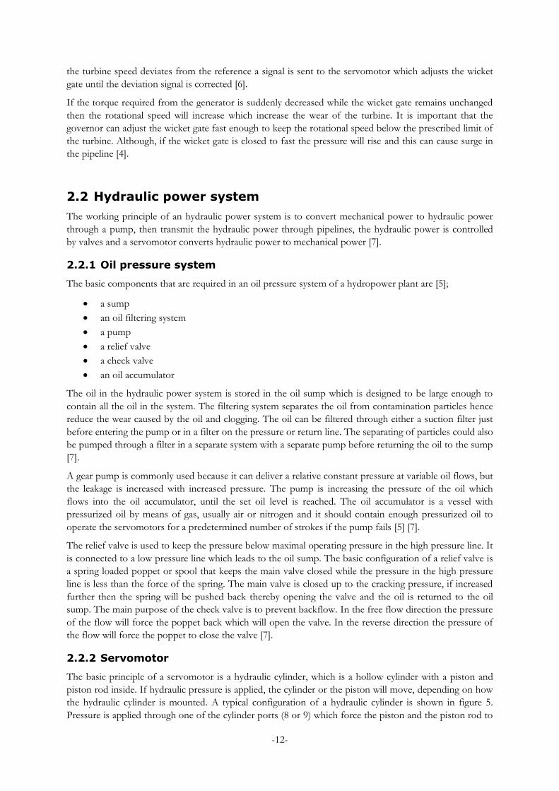
2.2.2 Servomotor

The basic principle of a servomotor is a hydraulic cylinder, which is a hollow cylinder with a piston and

piston rod inside. If hydraulic pressure is applied, the cylinder or the piston will move, depending on how

the hydraulic cylinder is mounted. A typical configuration of a hydraulic cylinder is shown in figure 5.

Pressure is applied through one of the cylinder ports (8 or 9) which force the piston and the piston rod to

-13-

move. This applies when the cylinder is fixated but if the piston rod is fixated instead then the cylinder is

forced to move. One piston stroke is the total length that the piston rod or the cylinder can be moved [7].

Figure 3, shows a typical configuration of a hydraulic cylinder [7].

2.3 Regulation mechanism

The regulation mechanism is controlled by the governor through the servomotors and the hydraulic

pressure system. The hydraulic pressure system supplies high pressure while the governor controls how

much pressurized oil that is supplied to the servomotors, hence controlling how far piston rod moves [5].

The principal layout of the guide vane and runner blade regulation differs and will be described separately.

2.3.1 Guide vane regulation

As mentioned above, the guide vane angle is regulated to increase or decrease the water flowing to the

turbine runner. In figure 4 the basic components of the regulation mechanism can be seen, where the red

parts are the top trunnion of the guide vanes which the levers are mounted on.

To adjust the angle of the guide vanes a force needs to be applied on the pin that connects the lever and

link. Force is applied from one or several servomotors to the operating ring which starts to rotate. From

the operating ring the force is transferred through a link to the lever which causes the guide vane to rotate.

There is only one operating ring but there should be as many links and levers as there are guide vanes.

If something like ice, stones etc. get stuck in between two guide vanes the servomotor will still apply force

and the guide vanes will try to close the gap between them and the pressure will increase until something

break. The regulation mechanism of the guide vanes are usually designed so that the link between the

operating ring and the lever will break when the force is too high [8].

-14-

Figure 4, shows a basic layout of the regulation mechanism of the guide vanes.

2.3.2 Runner blade regulation

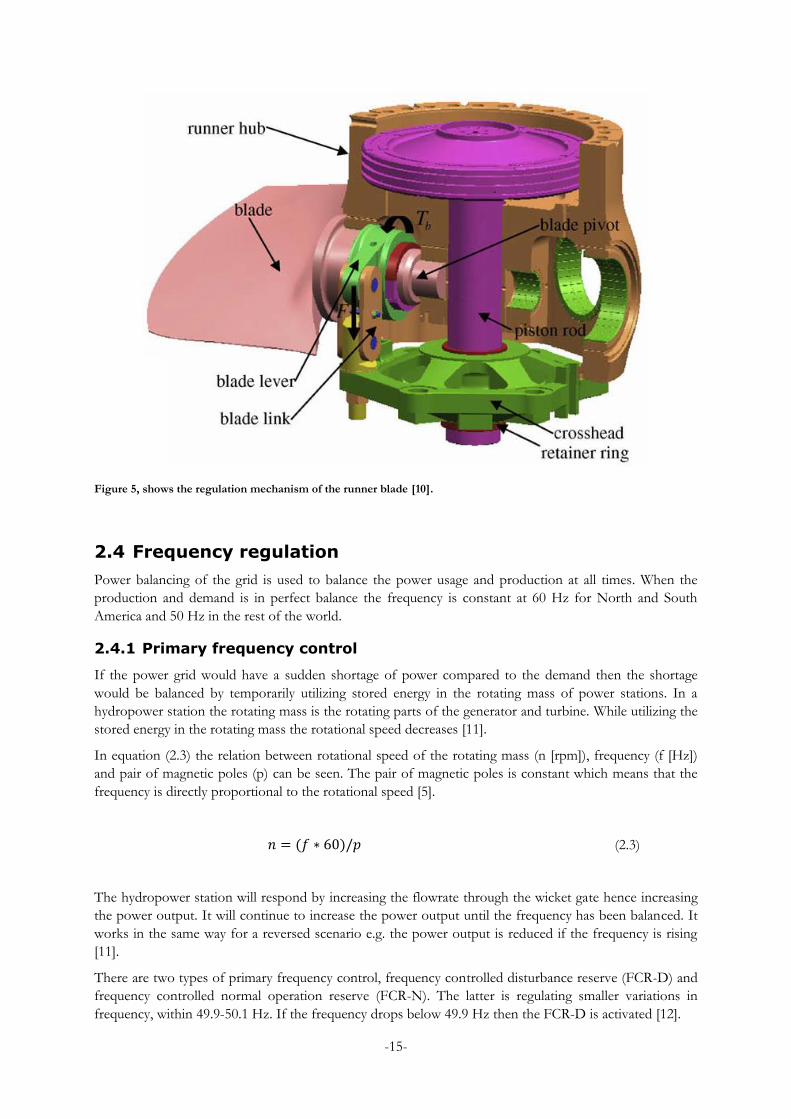
Figure 6 shows the regulation mechanism of a runner blade of a Kaplan turbine. It should be mentioned

that the layout of the regulation mechanism is individually designed in most cases, thus figure 6 is

representative for one turbine, but the working principle is the same in most cases. In figure 6 a Kaplan

turbine where the servomotor is placed upstream of the runner blades is illustrated. The servomotor could

also be placed downstream of the runner blades; this is a more recent design with the benefit of easier

access thus easier maintenance [9].

The runner hub is the casing of the turbine and seals of the inside mechanism from the flowing water

outside of the hub. The runner hub is filled with oil, water or air which acts as lubrication and corrosion

protection. All the areas where there is a potential for leakage are sealed to keep the water from

penetrating the hub and the fluid from escaping the hub. The Kaplan runner is classified as environmental

friendly if the hub is filled with water or air instead of oil [4] [9]. As in figure 6, the runner hub can be used

as the servomotors barrel in which the piston can move.

The purple part in figure 6 is the piston and piston rod and for a servomotor placed downstream of the

runner blades the piston and piston rod would be placed below the crosshead. The linkage between the

runner blade and the servomotor consists of the crosshead, a blade link, a blade lever and a blade pivot

(also called blade trunnion). The crosshead is mounted on to the piston rod and the blade link is the

connection between the crosshead and the blade lever. The blade lever is mounted on to the blade pivot

and converts the forces transmitted through the blade link into torque which rotates the blade.

In the both the upstream and the downstream configuration the hydraulic oil enters the servomotor

through concentric pipes inside of the turbine-generator shaft. At the top of these pipes the oil pressure

system is connected and is fixed to the piston in the other end. Since the concentric pipes are fixed to the

piston, the position of the pipes gives feedback on the movement in the regulation of the runner blade [8].

-15-

Figure 5, shows the regulation mechanism of the runner blade [10].

2.4 Frequency regulation

Power balancing of the grid is used to balance the power usage and production at all times. When the

production and demand is in perfect balance the frequency is constant at 60 Hz for North and South

America and 50 Hz in the rest of the world.

2.4.1 Primary frequency control

If the power grid would have a sudden shortage of power compared to the demand then the shortage

would be balanced by temporarily utilizing stored energy in the rotating mass of power stations. In a

hydropower station the rotating mass is the rotating parts of the generator and turbine. While utilizing the

stored energy in the rotating mass the rotational speed decreases [11].

In equation (2.3) the relation between rotational speed of the rotating mass (n [rpm]), frequency (f [Hz])

and pair of magnetic poles (p) can be seen. The pair of magnetic poles is constant which means that the

frequency is directly proportional to the rotational speed [5].

𝑛 = (𝑓 ∗ 60)/𝑝 (2.3)

The hydropower station will respond by increasing the flowrate through the wicket gate hence increasing

the power output. It will continue to increase the power output until the frequency has been balanced. It

works in the same way for a reversed scenario e.g. the power output is reduced if the frequency is rising

[11].

There are two types of primary frequency control, frequency controlled disturbance reserve (FCR-D) and

frequency controlled normal operation reserve (FCR-N). The latter is regulating smaller variations in

frequency, within 49.9-50.1 Hz. If the frequency drops below 49.9 Hz then the FCR-D is activated [12].

-16-

If the primary frequency reserve is fully activated, but the frequency is not yet balanced then other

measures are taken. First the export of electricity is regulated along with automatic shutdown of electric

boilers and heat pumps. Next step is automatic disconnection of loads on the demand side and the last

step is manually disconnection of loads [11].

2.4.2 Secondary frequency control

When the frequency has been stabilized it needs to be restored to the rated value and relieve the primary

resources, such operation is called secondary frequency control. A different power plant increase the

power output so that the used primary resource can be restored [11]. There are two main types of

secondary frequency control, frequency restoration reserve- automatic (FRR-A) and frequency restoration

reserve- manual (FRR-M). The former is used to restore the primary resources when the frequency

deviates from the rated frequency. FRR-M is used to regulate the frequency manually by increasing or

decreasing the power output on the grid [13].

2.4.3 Regulating power

The regulating power is defined as the change in power production from a hydropower station for a

certain change in frequency. The regulating power is measured in MW/Hz and if the regulating power is

set to 300 MW/Hz then the hydropower station will increase the power production with 30 MW if the

frequency drops with 0.1 Hz. Equation (2.4) shows the relation between frequency, regulating power (R)

and the power production.

𝐺 = 𝐺0 − 𝑅 ∗ (𝑓 − 𝑓0) (2.4)

G and G0 are the actual and rated power production [MW], f and f0 are the actual and rated frequency

[Hz]. From equation (2.4) it is shown that if the actual frequency is larger than the rated then the power

production will decrease and vice versa [11].

2.5 Dead-band and filtering systems

A dead-band is often used to reduce the number of movements in the regulating mechanism. The dead-

band can be placed in the turbine speed governor and adjusts the response to a deviation for the reference

value. For example if the governor detects a deviation in the frequency the governor will adjust the power

output, but with a dead-band in the governor the deviation will be set to zero if it is within the dead-band

range, hence reduce the number of adjustments made by the governor [14].

Voith Hydro has developed filtering system to reduce the number of movements in the regulating system.

It is a two measure system, where one filter is placed to suppress the noise in the frequency and one filter

is placed to reduce the adjustments of the runner blade angle. The first filter makes the governor follow

the frequency changes with high amplitudes or long durations. The second filter is used to quantizing the

runner blade position, i.e. divide the movements of the runner blade into steps and the angle will only be

adjusted if the change is larger than the step. Hence for changes smaller than the quantization steps the

power output will be adjusted only by the wicket gate leading to a deviation from the optimum relation

between the guide vane angle and the runner blade angle. Although with the right parameterization the

efficiency loss due to the deviation from the optimum relations can be neglected [15].

-17-

2.6 Jössefors hydropower station

Jössefors hydropower station was built in 1951 in Byälven in Sweden and has a net head of 25 m. It

consists of one unit which has a rated power of 25 MW with an average annual power production of 64.5

GWh. The turbine is a five-bladed vertical Kapan with rated power of 25.7 MW and 130 m3/s in rated

flow. The runner has a diameter of 4450 mm and rotates at 136 rpm. The servomotor in the runner is

supplied by a low pressure oil system (2 MPa) while the servomotor in the wicket gate is supplied by a

high pressure oil system (16 MPa).

-18-

3 Measurement on site

3.1 Preparations

Before the pressure measurements could be executed some material had to be purchased, the equipment

had to be tested and calibrated and some software had to be installed.

The material needed for the measurement was eight pressure transmitters, four for the servomotor

measurement, and four for the water pressure in the spiral and the water pressure in the draft tube. Two

different models were bought, one with a measurement span of -1 to 500 bars for the servomotor

measurement and one with a measurement span of -1 to 100 bars for the measurement in the waterway.

All of the transmitters’ measure gauge pressure, which means that the pressure is measured relative to the

atmospheric pressure. The pressure transmitter converts the pressure to a 4-20 mA signal, thus a data

acquisition unit was needed. The data acquisition unit can register a voltage signal; hence the mA signal

was converted to a voltage signal through a resistance. The voltage was registered, scaled to a pressure and

logged in ServiceLab.

The same type of cable was bought for both the power supply and the mA signal. The transmitters were

connected to a power source of 24 V with a 230 Ω resistance in series. Over the resistance the data

acquisition unit was connected and through an Ethernet cable it was connected to the computer, the

layout of the connecting scheme is shown in figure 6.

Figure 6, shows the connecting scheme of the pressure transmitter.

A special connecting cable was bought so that the pressure transmitters could be connected directly to the

computer (without the data acquisition unit) and with the supplied software the settings of the

transmitters could be changed. All the transmitters were calibrated and the measurement span was

adjusted to -1 to 250 bars for the ones measuring the servomotor pressure and -1 to 50 bars for the ones

measuring the water pressure.

The pressure transmitter has a ½ NPT female threads process connection and the process connections in

Jössefors are Minimess test points which have M16x2 threads, thus a transition between the process

connections was needed. It was a bit difficult to find one single coupling transition between the process

connections, thus the coupling transition consisted of firs a transition from ½ NPT female to 3/8” male

thread and then a test hose between the 3/8” male thread and the M16x2 thread.

-19-

3.2 Execution & data gathering

Jössefors hydropower station was available for measurements during two and a half days. The first day

was scheduled for rigging up the equipment, the second day was scheduled for the measurements and the

last half a day was intended as reserve time and taking down the equipment.

To set up the equipment was more time consuming than expected and at the end of the first day the

equipment was not completely installed. On the second day the installation of the equipment was finished,

but due to the time constraints the pressure measurements in the spiral was skipped and no test points for

the pressure measurements in the draft tube was found so those measurements were also skipped.

When everything was rigged and the pressure measurements could begin it was realized that the test

points used for measuring the servomotor pressure in the runner were the wrong ones. It was static and

too high for being the right pressure. The schematics over the oil pressuring system were examined trying

to find the right test points. It was unclear if the right test points even existed and the time was running

out, hence it was decided to continue with the measurements without the servomotor pressure in the

runner so that at least some data could be logged before taking the equipment down. Thus it was only the

servomotor pressure in the wicket gate that was logged, together with the active power, the frequency and

the percentage of opening of the wicket gate.

First the turbine speed governor was given a sinusoidal frequency, which was a 60 seconds frequency with

amplitude of 0.1 Hz. This means that in 60 seconds the frequency will changed from 50.1 Hz down to

49.9 Hz and back to 50.1 Hz. Then the turbine speed governor was connected to the frequency in the

grid. Last the pressure in the servomotor was logged during a stop and start sequence of the turbine.

Since no data on the servomotor pressure was acquired it had to be retrieved from somewhere else and

Voith hydro had done some previous measurements that could be used in this thesis. There are some

differences between the regulating mechanism and design of the turbine. The turbine has a newer design

with the servomotor located downstream of the runner blades with a high oil pressuring system (16 MPa).

In addition to the servomotor pressure; the active power and the opening percentage of the runner blades

had been logged, but not the frequency.

-20-

4 Calculation method

To calculate the stresses that the mechanical parts in the regulation mechanism is subjected to a model

which calculates the forces for each part is needed, this will be explained in this section. The calculation

model to determine the stresses and the life time expectations will also be explained here.

The advantage of using a simplified model as the one presented in this thesis is that it gives a fast and

reasonable result. Although some assumptions have to be made which reduces the accuracy of the result,

thus the stresses and life times calculated should mainly be used as estimations.

When the forces are calculated Peterson’s stress concentration factors are used which are considered to

have god accuracy. Especially the concentration factors calculated from the third edition since those have

been verified with Finite Element Method (FEM) [16].

4.1 Angles in the guide vane regulating mechanism

The definition of the guide vane angle is shown in figure 7. Where α is the angle between the center line of

the guide vane and the tangential line of the trunnion, i.e. the line 90° from the radius line. As can be seen

in figure 7 the angle of the guide vane is not zero in closed position. The rest of the angles in the guide

vane regulating mechanism are calculated from the angle of the guide vane.

Figure 7, shows the guide vane angle α and that it is the angle between the tangential line in the trunnion and the center line of the guide vane.

The feedback from the servomotor tells the governor the position of the servomotor piston which trough

linearization is translated to percentage of opening ΔA. This means that the angle of the guide vane has to

be translated from percentage of opening. A linearization can be made since the boundary conditions are

known, i.e. at 0% and 100% opening the angle of the guide vane is known, the difference between these

angles is Δα and is shown figure 8. The relation between the guide vane angle and the percentage opening

is shown in equation (3.1). The guide vane angle when the wicket gate is in closed position is α0.

-21-

𝛼 = 𝛼0 + ∆𝛼 ∗∆𝐴

100 (3.1)

Figure 8, shows the difference in guide vane angle between 0% and 100% opened positions, where the dashed figure represents 0% opened position.

The rest of the angles in the guide vane regulating mechanism and the distribution of the force on the link

pin are shown in figure 9, where;

α1 is the lever angle from the tangential line of the trunnion. This angle consists of the guide vane

angle and the fixed angle between the guide vane and the lever, since the latter is fixed α1 will

change as much as the guide vane angle

α2 is the angle between the lever and the link

α3 in the angle of the link

FT is the tangential force applied to each link. This force is calculated by equilibrium of moment

around the center of the operating ring, according to equation (3.2). Where r1 and r2 is the radius

to the servomotor and link connection on the operating ring respectively, Fs is the force applied

from the servomotor and z is the number of links

𝐹𝑆 ∗ 𝑟1 = 𝑧 ∗ 𝐹𝑇 ∗ 𝑟2 (3.2)

Fr is the radial force component in the link

Ft is the transvers force component in the link

-22-

Figure 9, shows the different angles in the guide vane regulation mechanism that are used to calculate the forces that the mechanical parts are subjected to.

As mentioned above α is calculated from the percentage of opening and since the angle between the guide

vane and the lever is fixed α1 is also determined from the percentage of opening. When the wicket gate is

opened or closed it also changes α2 and α3. These angles are calculated in MATLAB by first determine the

position of the connecting pin between the lever and the link, which is done by knowing the dimensions

of the lever and α1. Secondly the position of the connecting pin between the link and the operating ring is

at a constant radius from the center of the operating ring. In MATLAB the connection pin between the

link and the operating ring is adjusted iteratively until the length between the two connecting pins in the

link coincides with the real length, the iterative process is shown in figure 10. At this point the positions of

the mechanical parts has been determined it is now possible to calculate the angles required to translate

the force from the servomotor through the regulating mechanism.

-23-

Figure 10, shows the iterative process of finding the positioning of the connecting pin between the link and the operating ring. The red lines represent the real positioning of the lever (line A to B) and the link (line B to C) when the wicket gate is opened 0%, 50% and 100%. Each blue line represents the link length between the first and the last iteration.

4.2 Angles in the runner blade regulating mechanism

As showed in figure 2, the angle of the runner blade (from this point forward called φ) is measured from

the horizontal plane and the other angles will be calculated from φ. The blade trunnion and lever are

integrated and there will be a fixed angle between the lever and the blade, thus the lever will rotate with

the same angle as the blade. In figure 11 the angles used to calculate the forces through the runner

regulating mechanism is shown, where β1 is the angle between the runner blade and lever, β2 is the angle

between the lever and link, and β3 is the angle of the link measured from the vertical axis. Figure 11 also

shows the coordinate system placed at the center of the trunnion.

From the construction drawings of the runner blade and the trunnion with integrated lever β1 could be

determined. Knowing the lever angle and length the position of the connecting pin could be determined

in y and z coordinates. From the assembly drawings of the turbine the height between the center of the

blade trunnion and the crosshead lugs can be determined and so can the maximum stroke of the

servomotor. This means that the position of both the lever and crosshead lug is determined at the runner

blades maximum and minimum angle.

When the angle of the runner blade is adjusted the lever lug position is calculated and then through

iteration the position of the crosshead lug is determined. For each position of the crosshead lug the link

length is calculated and the deviation from the real link length in percent is calculated, while the deviation

is larger 0.1% (results in a deviation less than one mm) the iteration continues. When the position of the

crosshead lug is determined, β2 and β3 can be calculated.

-24-

Figure 11, shows the definition of the angles used to calculate the forces in the mechanical parts of the runner. The red part is the runner blade, the brown part is a part of the trunnion, the purple part is the lever, the blue part is the link, the green parts are the connecting pins and the yellow part is the crosshead.

4.3 Forces and stresses in the wicket gate

4.3.1 The lever

The force applied to the lever is shown in figure 12 and part a. shows that the force from the link is

divided into one radial force and one tangential force. The radial force will subject the lever to tension

stresses and the tangential force will subject it to a bending force which will cause bending stresses. As can

be seen the radial force is much smaller than the tangential force, thus it will be neglected in the stress

calculations of the lever. The cross section of the lever is shown in part b. of figure 12 with the shear

forces displayed.

Figure 12, shows the geometry of the lever, in a. a top view shows how the link force (Flink) is divided into one radial (Fr) and one tangential force (Ft) and the radius to the center line of the lever (r). In part b. the shear forces F1, F2 and F3 are shown along with the tangential force and the point of the moment around the z-axis. Part b. also shows the definitions of h, b, c, t and e.

-25-

The bending stress σb,nom is calculated according to equating (3.3), where Mb [Nm] is the bending moment

at the furthest point from the neutral axis, I [m4] is the moment of inertia around the symmetry axis and c

[m] is the distance from the edge to the center line of the lever [16]. I is calculated according to equation

(3.4) which only depends on the geometry of the cross section, where c is mentioned before and t [m], h

[m] and b [m] are all shown in figure 12 b. [17]. Equation (3.5) calculates the maximum stress, either

bending or tension. Kt is the stress concentration factor which in some cases is already calculated and can

be determined from charts or in other cases it needs to be calculated, as in this case. Equation (3.6) is used

to calculate the stress concentration factor for a curved beam where I, b and c has already been mentioned

and r [m] is the radius of the centerline in the lever and B is a constant of 0.5 for cross sections that are

not circular or elliptical [16]. It should be noted that the cross section has been simplified and the cross

section actually used for the calculations in the lever is dotted in figure 12 b.

𝜎𝑏,𝑛𝑜𝑚 =𝑀𝑏𝐼𝑐⁄ (3.3)

𝐼 =1

12𝑡ℎ3 + 2𝑏𝑡𝑐2 + 2

1

12𝑏𝑡3 (3.4)

𝜎𝑚𝑎𝑥 = 𝐾𝑡 ∗ 𝜎𝑛𝑜𝑚 (3.5)

𝐾𝑡 = 1.00 + 𝐵 ∗ (𝐼

𝑏∗𝑐2) ∗ (

1

𝑟−𝑐+1

𝑟) (3.6)

The shear forces shown in figure 12 b. needs to be calculated so that the average shear stress in the cross

section can be determined. F1, F2 and F3 are calculated using the equilibrium equations (3.7) to (3.9),

where e [m] is the lever arm of the tangential force [17]. The shear stress τ [Pa] due to the three shear

forces are calculated according to equation (3.10) where T [N] represents the shear forces and A [m2] is

the cross section on which the shear force act [18]. The average of the three shear stresses is calculated

and is the shear stress used to evaluate the equivalent stress described below.

∑𝐹𝑥 = 𝐹2 − 𝐹1 = 0 (3.7)

∑𝐹𝑦 = 𝐹𝑡 − 𝐹3 = 0 (3.8)

∑𝑀𝑧 = 𝐹𝑡 ∗ 𝑒 − 𝐹1 ∗ ℎ = 0 (3.9)

𝜏 =𝑇

𝐴 (3.10)

In the section where there is a change in cross section area the pin will be subjected to both bending and

shear stress, thus the equivalent stress σeq is calculated according to von Mises criterion. The energy of the

combined stresses is translated into a pure tension stress with the same amount of energy. The equivalent

stress for plane stress, i.e. stress in two dimensions, is calculated according to equation (3.11) [16]. Where

-26-

σmax,1 and σmax,2 are the maximum stress due to tension and moment, and τmax,3 is the maximum shear

stress.

𝜎𝑒𝑞 = √(𝜎𝑚𝑎𝑥,1 + 𝜎𝑚𝑎𝑥,2)2+ 3𝜏𝑚𝑎𝑥,3

2 (3.11)

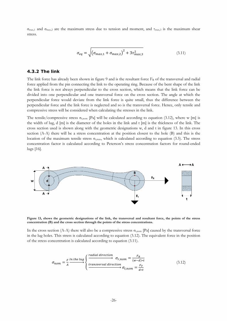
4.3.2 The link

The link force has already been shown in figure 9 and is the resultant force FR of the transversal and radial

force applied from the pin connecting the link to the operating ring. Because of the bent shape of the link

the link force is not always perpendicular to the cross section, which means that the link force can be

divided into one perpendicular and one transversal force on the cross section. The angle at which the

perpendicular force would deviate from the link force is quite small, thus the difference between the

perpendicular force and the link force is neglected and so is the transversal force. Hence, only tensile and

compressive stress will be considered when calculating the stresses in the link.

The tensile/compressive stress σr,nom [Pa] will be calculated according to equation (3.12), where w [m] is

the width of lug, d [m] is the diameter of the holes in the link and t [m] is the thickness of the link. The

cross section used is shown along with the geometric designations w, d and t in figure 13. In this cross

section (A-A) there will be a stress concentration at the position closest to the hole (B) and this is the

location of the maximum tensile stress σt,max, which is calculated according to equation (3.5). The stress

concentration factor is calculated according to Peterson’s stress concentration factors for round-ended

lugs [16].

Figure 13, shows the geometric designations of the link, the transversal and resultant force, the points of the stress concentration (B) and the cross section through the points of the stress concentrations.

In the cross section (A-A) there will also be a compressive stress σt,nom [Pa] caused by the transversal force

in the lug holes. This stress is calculated according to equation (3.12). The equivalent force in the position

of the stress concentration is calculated according to equation (3.11).

𝜎𝑛𝑜𝑚 =𝐹

𝐴

𝐼𝑛 𝑡ℎ𝑒 𝑙𝑢𝑔→

𝑟𝑎𝑑𝑖𝑎𝑙 𝑑𝑖𝑟𝑒𝑐𝑡𝑖𝑜𝑛→ 𝜎𝑟,𝑛𝑜𝑚 =

𝐹𝑅(𝑤−𝑑)∗𝑡

𝑡𝑟𝑎𝑛𝑠𝑣𝑒𝑟𝑠𝑎𝑙 𝑑𝑖𝑟𝑒𝑐𝑡𝑖𝑜𝑛→ 𝜎𝑡,𝑛𝑜𝑚 =

𝐹𝑇

𝑑∗𝑡

(3.12)

-27-

4.3.3 The connecting pins

There are three pins in the wicket gate, one connecting the link and lever, one connecting the link and

operating ring and one connecting the operating ring and the servomotor. The first and the second

mentioned pins are mounted in the same way, with the link at the top part of the link and the lever or the

operating ring mounted at the bottom part. This type of pins is shown in figure 14.b. The remaining pin

has the servomotor connected to the middle part of the pin and the operating ring connected at the upper

and the bottom part, as shown in figure 14 a.

It can be seen in part a. of figure 14 that the pin will have one force from the servomotor and two forces

from the operating ring. Part b. of figure 14 shows the force from the link in the upper part and the force

from the lever or operating ring at the lower part of the pin.

Figure 14, shows the forces applied to the pins in the wicket gate, a. shows the pins connected to the operating ring and b. shows the pin connecting the link and lever.

These forces will cause bending and shear stress in the pins. The bending stress σb,nom [Pa] is calculated for

a circular cross section according to equation (3.13), where Mb [Nm] is the bending moment and d [m] is

the diameter. Due to the change in diameter there will be a stress concentration at the fillet and the

maximum bending stress σb,max [Pa] is calculated according to equation (3.5). The stress concentration

factor is calculated according to Peterson’s Stress Concentration Factors [16].

𝜎𝑏,𝑛𝑜𝑚 =32∗𝑀𝑏

𝜋∗𝑑3 (3.13)

The shear stress in the pins is calculated according to equation (3.10). Note that for the pins that are

connected to the operating ring T is equal to the applied force from the servomotor or the counter force

from the link divided by two while it is equal to the applied force in the pin connecting the link and lever.

4.4 Forces and stresses in the runner

4.4.1 The lever

The lever is integrated to the blade trunnion but only the stresses in the lever arm will be considered, this

since calculation reports made by Voith Hydro shows that the highest stresses exists in the lever arm. The

stresses in the lever arm will be calculated from the link force applied to the lug in the lever arm. There

will be a small force component in the radial direction of the lever, but most of the link force will be

applied in the transversal direction of the lever, this is shown in figure 15.

-28-

Figure 15, shows the force components applied from the link to integrated trunnion and lever. In cross section (A-A) there will be bending, shear and tension/compressive stresses and at position B there will be a stress concentration due to the lug.

There will be a stress concentration at the edge of the lug hole due to the radial link force and a stress

concentration at the base of the lever due to both the radial and transversal link force. The position of

stress concentrations in the lug holes (B) and the cross section (A-A) are shown in figure 15. In cross

section (A-A) there will be a bending stress and shear stress due to the transversal link force and a

tension/compressive stress due to the radial link force. The bending stress is calculated for a rectangular

cross section according to equation (3.14), where d [m] is the width and h [m] is the thickness [16]. The

shear stress is calculated according to equation (3.10) and the tension/compressive stress is calculated

according to equation (3.12). The stress concentration factor in the lug is calculated according to

Peterson’s stress concentration factors and the nominal stress in the lug is calculated according to (3.12)

(both radial and transversal direction).

𝜎𝑏,𝑛𝑜𝑚 =6𝑀𝑏

ℎ𝑑2 (3.14)

4.4.2 The link

The force in the link is applied from the crosshead in vertical direction and is divided into a radial and a

tangential link force. Like the link in the wicket gate the link lugs will cause a stress concentration and in

the same point the tangential force will cause a compressive force, thus the stress and stress concentration

will be calculated in the same way as the link in the wicket gate. It should be noted that there are two

parallel links (one outer and one inner) for each runner blade, thus each link will be subjected to half of

the force applied from the crosshead. In the middle of the link there is another hole which also causes a

stress concentration, but due to a much smaller diameter than the lug holes this will not be the area of the

largest stress concentration in the link. Another difference from the link in the wicket gate is that the lug

holes differ in diameter. The inner link has one diameter for both lug holes but the outer link has two

different diameters and between the inner and outer link the diameters of the lug holes are not the same

either. This means that there are three different diameters of the lug holes in the links; hence the stress

concentrations will be different. The lug hole with the largest stress concentration factor will give the

largest stress concentration.

-29-

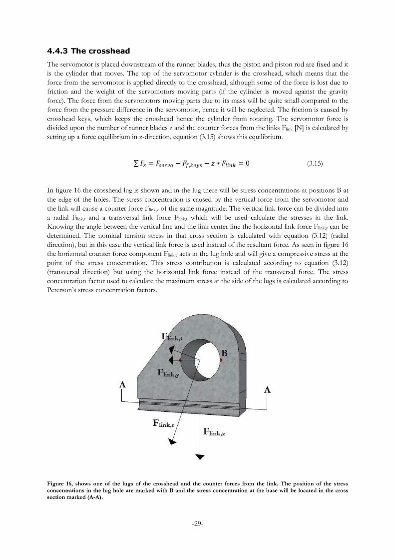
4.4.3 The crosshead

The servomotor is placed downstream of the runner blades, thus the piston and piston rod are fixed and it

is the cylinder that moves. The top of the servomotor cylinder is the crosshead, which means that the

force from the servomotor is applied directly to the crosshead, although some of the force is lost due to

friction and the weight of the servomotors moving parts (if the cylinder is moved against the gravity

force). The force from the servomotors moving parts due to its mass will be quite small compared to the

force from the pressure difference in the servomotor, hence it will be neglected. The friction is caused by

crosshead keys, which keeps the crosshead hence the cylinder from rotating. The servomotor force is

divided upon the number of runner blades z and the counter forces from the links Flink [N] is calculated by

setting up a force equilibrium in z-direction, equation (3.15) shows this equilibrium.

∑𝐹𝑧 = 𝐹𝑠𝑒𝑟𝑣𝑜 − 𝐹𝑓,𝑘𝑒𝑦𝑠 − 𝑧 ∗ 𝐹𝑙𝑖𝑛𝑘 = 0 (3.15)

In figure 16 the crosshead lug is shown and in the lug there will be stress concentrations at positions B at

the edge of the holes. The stress concentration is caused by the vertical force from the servomotor and

the link will cause a counter force Flink,z of the same magnitude. The vertical link force can be divided into

a radial Flink,r and a transversal link force Flink,t which will be used calculate the stresses in the link.

Knowing the angle between the vertical line and the link center line the horizontal link force Flink,y can be

determined. The nominal tension stress in that cross section is calculated with equation (3.12) (radial

direction), but in this case the vertical link force is used instead of the resultant force. As seen in figure 16

the horizontal counter force component Flink,y acts in the lug hole and will give a compressive stress at the

point of the stress concentration. This stress contribution is calculated according to equation (3.12)

(transversal direction) but using the horizontal link force instead of the transversal force. The stress

concentration factor used to calculate the maximum stress at the side of the lugs is calculated according to

Peterson’s stress concentration factors.

Figure 16, shows one of the lugs of the crosshead and the counter forces from the link. The position of the stress concentrations in the lug hole are marked with B and the stress concentration at the base will be located in the cross section marked (A-A).

-30-

At the base of the lug there will also be a stress concentration since the horizontal link force will cause a

bending stress and the vertical link force will cause a tension/compressive stress in that cross section. The

bending stress is calculated for a rectangular cross section according to equation (3.14). The tension stress

is calculated according to (3.12) with the rectangular cross section at the base.

There is also a fillet where the crosshead is mounted upon the piston rod, but if the piston rod is

considered as a solid then the diameter and cross section is quite large thus the nominal stress at the cross

section of that fillet is quite small. Even with a stress concentration factor the stress would not be larger

than that in the lug, thus the stress at that fillet will not be calculated.

4.4.4 The crosshead keys

As mentioned above the crosshead keys are keeping the crosshead and the rest of the cylinder from

rotating inside the hub. The counter force component in horizontal direction applied from the link to the

cross head will cause a moment force around the turbine axis which is absorbed by three crosshead keys.

The force applied to the keys Fkey [N] is calculated by setting up moment equilibrium around the piston

rod according to equation (3.15). Where zlink and zkey are the number of links and keys respectively and rlink

[m] and rkey [m] are the lever arm to the link and key respectively.

∑𝑀𝑧 = 𝑧𝑙𝑖𝑛𝑘𝐹𝑙𝑖𝑛𝑘,𝑦𝑟𝑙𝑖𝑛𝑘 − 𝑧𝑘𝑒𝑦𝑠𝐹𝑘𝑒𝑦𝑟𝑘𝑒𝑦 = 0 (3.15)

The key force will cause a bending stress and a shear stress which are calculated according to equation

(3.14) and (3.10) respectively and the equivalent stress will be calculated according to (3.11). The keys are a

part of the runner hub and the stresses will be largest at the base of the keys.

4.4.5 The connecting pins

In the runner there are two connecting pins and are mounted in the link holes, one in each. As mentioned

before there are two parallel links in the regulating mechanism for each runner blade, thus the connecting

pins will be subjected to the link force at two points, half the force at the top and half of the force at the

bottom. In the middle of the connecting pins is either the lever or the crosshead connected, thus the

loading situation is similar to the connecting pins in the operating ring, which is shown in figure 17. Hence

the bending stress, the shear stress, the equivalent stress will be calculated in the same way, using

Peterson’s stress concentration factors to determine the maximum bending stress.

-31-

Figure 17, shows the pins connecting the link to the lever and the link to the cross head.

4.5 Fatigue and life time calculations

4.5.1 Rain-flow count

The rain-flow count method determine the stress range for each load cycle in a load sequence and for

counts how many load cycles of each stress range that occurs. The load sequence should be displayed in a

diagram with stress as a function of time and it should be tilted 90 degrees so that the time axis is pointing

downwards. A raindrop is dropped from the top of the sequence at a maximum or a minimum value. A

raindrop should be dropped from each maximum and each minimum point within the sequence. The

raindrop will keep running along the sequence until it either passes a maximum (if it starts from a

maximum point) or a minimum (if it starts from a minimum point) equal to the starting value (or larger

respectively smaller than the starting value). The raindrop will also stop if it encounters a flow path of a

previous raindrop. The flow paths are then coupled together to create load cycles [18].

4.5.2 Palmgren-Miner rule

If the load sequence and the material data of a body are known then the accumulative fatigue damage can

be calculated with the Palmgren-miner rule. The rain-flow count method can be used to calculate the

number of cycles of a specific stress range that the material is subjected to during the load sequence. The

material data is used to determine how many cycles of that stress range the material can withstand before

failure. The relative fatigue damage can then be calculated with the equation (3.16).

∑𝑛𝑖

𝑁𝑖= 𝐶 (3.16)

The equation is summarizing all the fatigue damage for the whole stress amplitude spectrum, where ni is

the number of cycles at a specific stress range and Ni is the number of cycles the component can

-32-

withstand at that stress range. The component C is a constant, it is common to use the value 1. The

accumulated fatigue damage is the inverse of the estimated life time, measured in the amount of time

periods left. This means that if the time period is 1 year than inverse of the accumulated fatigue damage is

the number of years left, but if the time period is 10 years than the inverse is the number of 10 years

periods left [19].

4.5.3 S-N curve

In high cycle fatigue cases, when there are a large amount of cycles N (usually more than 105 cycles), the

stress amplitude S versus N are usually plotted in an S-N curve (also known as Wöhler curve) as shown in

figure 18. The lines represent the fatigue limit of a certain material and if a stress sequence is above the

material will theoretically fail due to fatigue. These curves are either constructed through calculation or

tests. For some materials there will be an endurance limit, which means that if the stress amplitude is kept

below the fatigue limit when the line has flattened out the material can withstand unlimited number of

cycles. In figure 18 the endurance limit is around 320 MPa for 1045 Steel [20].

Figure 18, shows an S-N curve with and without an endurance limit [20].

In this thesis the S-N curves will be calculated for the materials investigated. The S-N curves will be

calculated according to “Plåthandboken; Att konstruera och tillverka i höghållfast stål” guidelines. It is a

guide line from SSAB, where the method used in this thesis for calculating the S-N curve is based on tests

of different classification joints.

The number of cycles N that a certain steel material can withstand at a certain stress range ∆σ [MPa] is

calculated according to equation (3.17). FAT [MPa] is a constant which depends on the classification of

the material joints. For example if a component has been welded together it will have a different FAT-

value than if the component was manufactured in one piece. The material joint constant will also differ

between different surface treatments. The slope of the curve is denoted m and it has a value of 3 for

welded joints and 5 for basic materials. For constructions which are not significantly affected of or are

protected against corrosion the endurance limit is used, but when there is a risk of corrosion or when the

accumulative damage is calculated the endurance limit is not used. In the case of not using the endurance

limit, the line created by equation (3.17) is used for all stress ranges.

-33-

𝑁 = 2 ∗ 106 (𝐹𝐴𝑇

∆𝜎)𝑚

(3.17)

The stress range used to evaluate how many cycles a component can take until fatigue failure is defined as

the difference between the maximum and the minimum value in a cycle. The maximum and minimum

nominal stresses can be calculated using super position (adding the stresses together), for example adding

the stresses due to bending and tension [21].

-34-

5 Results

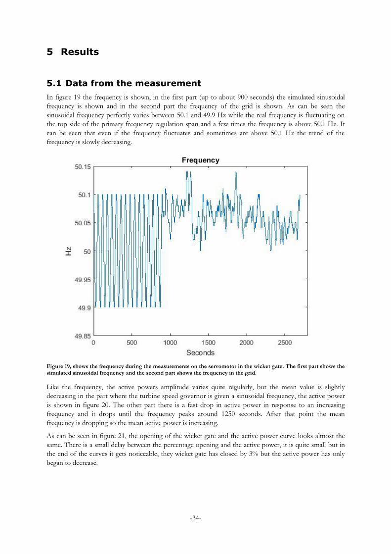
5.1 Data from the measurement

In figure 19 the frequency is shown, in the first part (up to about 900 seconds) the simulated sinusoidal

frequency is shown and in the second part the frequency of the grid is shown. As can be seen the

sinusoidal frequency perfectly varies between 50.1 and 49.9 Hz while the real frequency is fluctuating on

the top side of the primary frequency regulation span and a few times the frequency is above 50.1 Hz. It

can be seen that even if the frequency fluctuates and sometimes are above 50.1 Hz the trend of the

frequency is slowly decreasing.

Figure 19, shows the frequency during the measurements on the servomotor in the wicket gate. The first part shows the simulated sinusoidal frequency and the second part shows the frequency in the grid.

Like the frequency, the active powers amplitude varies quite regularly, but the mean value is slightly

decreasing in the part where the turbine speed governor is given a sinusoidal frequency, the active power

is shown in figure 20. The other part there is a fast drop in active power in response to an increasing

frequency and it drops until the frequency peaks around 1250 seconds. After that point the mean

frequency is dropping so the mean active power is increasing.

As can be seen in figure 21, the opening of the wicket gate and the active power curve looks almost the

same. There is a small delay between the percentage opening and the active power, it is quite small but in

the end of the curves it gets noticeable, they wicket gate has closed by 3% but the active power has only

began to decrease.

-35-

Figure 20, shows the active power during the measurements of the servomotor in the wicket gate. The first and evenly distributed part is during the sinusoidal frequency and the other part is during the frequency in the grid.

Figure 21, shows the percentage of opening of the wicket gate and it follows almost the same curve as the active power.

-36-

The pressure in the wicket gate servomotor is shown in figure 22, where the blue line is the pressure on

the opening side and the red line is the pressure on the closing side. Even here the first part varies more

evenly for both pressure sides but the difference between the pressure when operated with a sinusoidal

frequency and the grid frequency are not as clear as for the wicket gate opening and the active power. It

can be seen that the grid frequency leads to a more stochastic pattern, but the amplitudes are almost the

same for many of the cycles and so is the mean value. It can also be seen that for most of the changes in

the wicket gate opening the pressure spans are the same, i.e. the large wicket gate openings of about 4%

results in almost the same pressure increase as the smaller once around 1%.

The opening pressure is always larger than the closing pressure in the sequence shown in figure 22. This is

a result of two things, on the opening side the piston rod is connected to the piston, hence reducing the

effective area to which the pressure is applied thus to achieve the same force from the closing and

opening side the opening pressure has to be larger. The second reason is that the guide vanes are self-

closing, which means that the pressure from the water will try to close the guide vanes. Thus by just

reducing the opening pressure the water pressure will close the guide vanes without any additional

pressure on the closing side of the servomotor.

Figure 22, shows the pressure in the servomotor in the wicket gate, the blue line is the opening pressure and the red line is the closing pressure.

5.2 Provided data

Since the measurements did not turn out as expected some data had to be retrieved from somewhere else.

From Voith an 11 hour measurement sequence was provided, where the active power, the runner blade

angle and the pressure in the servomotor had been logged.

The whole sequence of measured active power is shown in figure 23 and an hour sequence is shown in

figure 24. Due to frequency regulation the active power is constantly varying which is seen in figure 24.

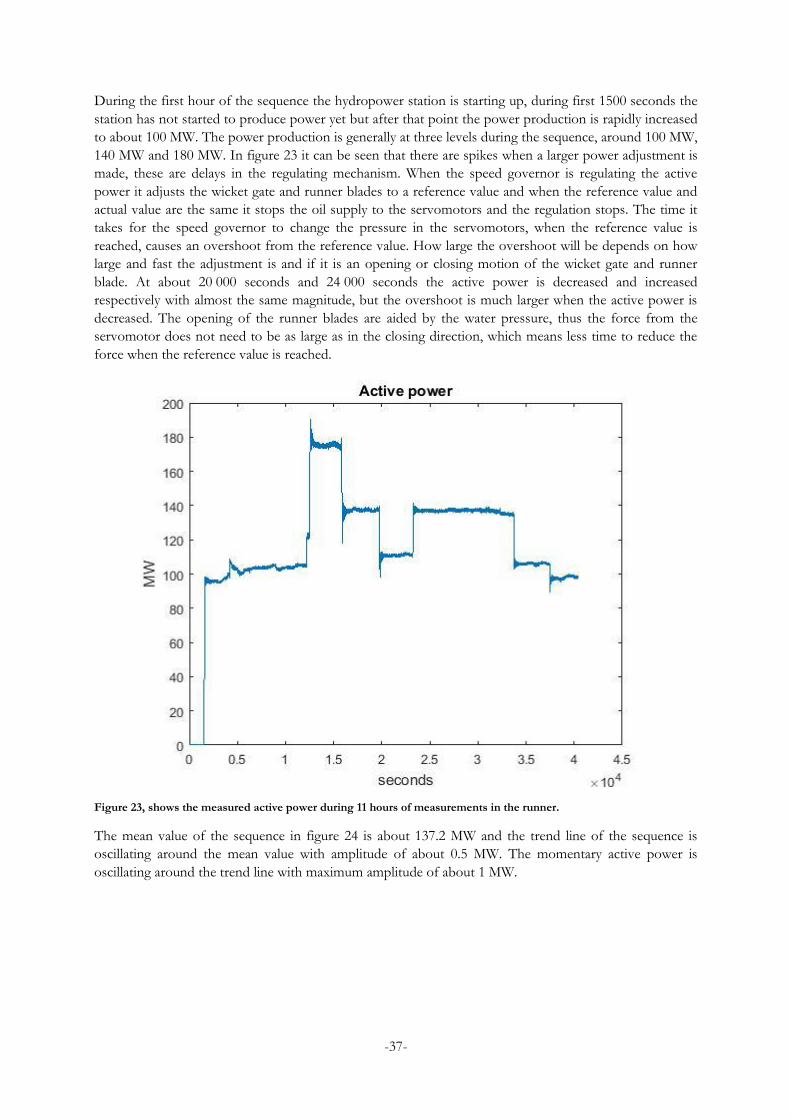
-37-

During the first hour of the sequence the hydropower station is starting up, during first 1500 seconds the

station has not started to produce power yet but after that point the power production is rapidly increased

to about 100 MW. The power production is generally at three levels during the sequence, around 100 MW,

140 MW and 180 MW. In figure 23 it can be seen that there are spikes when a larger power adjustment is

made, these are delays in the regulating mechanism. When the speed governor is regulating the active

power it adjusts the wicket gate and runner blades to a reference value and when the reference value and

actual value are the same it stops the oil supply to the servomotors and the regulation stops. The time it

takes for the speed governor to change the pressure in the servomotors, when the reference value is

reached, causes an overshoot from the reference value. How large the overshoot will be depends on how

large and fast the adjustment is and if it is an opening or closing motion of the wicket gate and runner

blade. At about 20 000 seconds and 24 000 seconds the active power is decreased and increased

respectively with almost the same magnitude, but the overshoot is much larger when the active power is

decreased. The opening of the runner blades are aided by the water pressure, thus the force from the

servomotor does not need to be as large as in the closing direction, which means less time to reduce the

force when the reference value is reached.

Figure 23, shows the measured active power during 11 hours of measurements in the runner.

The mean value of the sequence in figure 24 is about 137.2 MW and the trend line of the sequence is

oscillating around the mean value with amplitude of about 0.5 MW. The momentary active power is

oscillating around the trend line with maximum amplitude of about 1 MW.

-38-

Figure 24, shows the active power during a one hour sequence during the measurements in the runner. The data was logged during frequency regulation and the trend line is oscillating around the mean of the sequence with amplitude of 0.5 MW. From the trend line the active power varies with maximum amplitude of 1 MW.

The angle of the runner blade is shown in figure 25, the trend lines for the active power and the runner

blade angle are very similar but there are almost no oscillations from the trend line of the runner blade

angle. During the same hour sequence shown in figure 24 the runner blade changes angle in two cycles

(like the trend line of the active power) with the amplitude of 0.1 degrees, which is a change of about 0.3%

of the total angle span. Thus, by changing the active power with about 1 MW results in a runner blade

adjustment of 0.2 degrees.

-39-

Figure 25, shows the runner blade angle during the 11 hour sequence.

In figure 26 and 27 the opening and closing pressure respectively is shown. It can be seen that the opening

and closing pressure are changing in opposite direction of one another, i.e. when the opening pressure is

increasing the closing pressure is decreasing. The pressure on the opening side is generally larger, changing

between 6 and 14 MPa while the closing pressure changes between 4 and 12 MPa, which is due to the

difference in effective area as described for the servomotor pressure in the wicket gate.

There are four time points where opening side pressure is lower than the rest of the time, where the

pressure is around 4 MPa and this is due to a fast and large change in runner blade angle. In figure 26 at it

can be seen that at the same time points the closing pressure is high, around 13 MPa at the first point and

a little less than 12 MPa at the rest. Thus, the closing force is largest during these four time points and

looking at those points in figure 23 it can be seen that at least three of those four are the points where the

active power overshoots the reference value. The same points show that the runner blade angle also

overshoots the reference value in figure 25. At the first of these time points the blade angle has been

reduces with about 13 degrees and has overshoot the reference value with about 4 degrees.

The same hour sequence that was shown for the active power is shown for the opening and closing

pressure in figure 28. It can be seen that the pressure is changing opposite to one another and that both

sides change pressure with about 6 MPa. That represents 37.5% of the total pressure span for each side.

The opening pressure of the servomotor changes pressure in two cycles as the trend line of the active

power and runner blade angle, while the closing pressure side changes pressure in two cycles but in

opposite direction. Thus, to increase the active power the runner blade and the opening pressure are

increased while the closing pressure is decreased.

-40-

Figure 26, shows the opening pressure in the runner servomotor.

Figure 27, shows the closing pressure in the runner servomotor.

-41-

Figure 28, shows the opening and closing pressure in the servomotor during the same hour sequence shown for the active power.

5.3 Forces in the wicket gate

Except for the force applied from the servomotor the forces in the wicket gate are quite small, due to the

many guide vanes. As can be seen in figure 29 the servomotor force in this sequence reaches a maximum

value of about 120 kN and the maximum forces is divided upon 24 guide vanes which leads to quite small

forces in the regulating mechanism of each guide vane. A spike can be noticed which results in a

servomotor force of 160 kN which is considered as a measurement error. At all other points logged

during the measurements with the simulated frequency the opening and closing pressure increase at the

same time, but at that spike the logged closing pressure does not increase which causes the spike. Even

when maximum pressure is applied to the closing side, the servomotor force per guide vane would only be

about 30 kN, and that does not happen so often in a hydropower station. In table 1 the minimum and

maximum forces in the link and lever are displayed and the forces are quite small in all directions.

Table 1, shows the minimum to maximum forces in the link and lever

Component Radial [kN] Tangential [kN]

Link 1.5-4.5 0.7-2.0

Lever (-0.2)- (-0.8) 1.2-4.2

As long as there is no need for a fast closing of the wicket gate the water pressure will be used to close the

wicket gate in the way described above. This can be seen in figure 29, where the servomotor force in the

-42-

sequence is always positive because the force from the opening side is always larger than the force from

the closing side. As mentioned above it can be seen that regardless if there is a 4% or a 1% wicket gate

adjustment the applied force are almost the same.

Figure 29, shows the force from the servomotor in the wicket gate, it is always positive which means that the force from the opening side is always larger than the closing side in this sequence.

5.4 Forces in the runner

The servomotor force in the runner is shown in figure 30; the servomotor force has been divided upon

the five runner blades. The movement of the crosshead is defined to be positive when moving upwards

and vice versa. This means when the servomotor force is positive it is opening the runner blade and

closing it when the force is negative.

The force is distributed around a mean value of 100 kN with the maximum opening force of about 1500

kN and the maximum closing force of about 1700 kN during normal operation. Above it was mentioned

that at four points there was a large and fast reduction of the blade and at these points the larges closing

pressure occurs. Looking at these points in figure 30 shows that the closing force when the blade angle

was reduced 13 degrees is about 2250 kN and around 2000 kN at the three other points.

In figure 31 the servomotor force is shown for the same hour sequence as the active power. During that

small blade angle change the servomotor force is changing with the amplitude of 1250 kN. At the top,

somewhere around 27000-27400 seconds, the larger variations changes with about 100 to 250 kN.

Between 26500 and 27000 seconds the servomotor force is changed from about -1250 kN to 1250 kN

which results in a 0.2 degrees change of the runner blade angle. Thus, a large change like 13 degrees

resulted in a drop of about 40 MW which is 56.25 kN/MW while a small change like 0.1 degrees resulted

-43-

in a drop of 0.5 MW which is 2500 kN/MW. It can be seen that these small changes are more harmful

compared to what the gain form them are.

The rest of the forces in the runner blade regulating mechanism, follow the same curve as the servomotor

force and the estimated force spans (during most of the operation) are shown in table 2. However the

radial lever force will increase with increasing blade angle. For example if the same link force would be

applied when β2 (figure 11) is 80 degrees and when it is 70 degrees then the radial lever force will be twice

as large in the latter case. During most of the operation β2 is between 80-90 degrees but when the runner

blade is almost fully opened, between 12500 and 16000 seconds, β2 is around 70 degrees which results in

an increased radial lever force. During these seconds the radial lever force varies between -600 and 350

kN.

Table 2, shows the radial and transversal force spans in the link and lever during most of the operation.

Component Radial force [kN] Transversal force [kN]

Link (-1700)-1500 (-400)-300

Lever (-200)-200 (-1700)-1500

Figure 30, shows the servomotor force in the runner divided upon the five runner blades.

-44-

Figure 31, shows the servomotor force during the same hour sequence that the active power was shown.

5.5 Stresses in the wicket gate

Since the forces in the wicket gate was quite small it was expected that the stresses would be small as well.

Von Mises equivalent stress has been calculated in the stress concentration areas mentioned in section 4.3

for the lever, link and the connecting pins. The equivalent stresses in the lever, link and the connecting

pins, except the one connecting the servomotor to the operating ring, are shown in table 3.

Table 3, shows the maximum and minimum von Mises equivalent stresses in the link, lever, connecting pin between the lever and link and the connecting pin between the link and operating ring.

Component Min. Eq. Stress [MPa] Max. Eq. Stress [MPa]

Lever 0.5 1.4

Link 1.5 4.4

Connecting pin lever to link 0.8 2.3

Connecting pin link to operating ring 0.8 2.3

The equivalent stresses in the connecting pin between the servomotor and the operating ring is shown in

figure 32. It can be seen that the equivalent stresses are higher in this connecting pin, which was expected

since the force applied to it comes directly from the servomotor before the force is divided upon the

guide vanes. The mean equivalent stress is 42 MPa with estimated amplitude of 22 MPa and this will give a

stress range of 44 MPa. It can be seen that the majority of the stress cycles has a stress range of around 40

MPa even the smaller adjustments of the wicket gate opening.

-45-

Since the stresses are so low in all the components shown in table 3 no fatigue damage will be calculated

on those components and even though the stresses are higher in the connecting pin between the

servomotor and the operating ring the fatigue damage will not be evaluated in this component either.

Figure 32, shows the von Mises equivalent stresses in the connecting pin between the servomotor and the operating ring.

5.6 Stresses in the runner

The maximum von Mises equivalent stress was calculated for all the components and positions mentioned

in section 4.4 and the results are shown in table 4. In the lever the maximum equivalent stress will be in

the lug and in the crosshead it will also be in the lug. The rest of the components only had one position

with stress concentration, hence that will be the positions of maximum equivalent stress.

In figure 33 to figure 37 the combined normal stresses for the lever lug, link, crosshead lug, crosshead

keys and connecting pins are shown respectively during the 11 hour measuring sequence. The normal

stresses are used since the shear stress has been neglected. When comparing the equivalent stresses to the

normal stresses it showed that the contribution from the shear stresses was about 5%, hence it was

neglected.

It can be seen that the stresses follows almost the same curve in all the components but at different

magnitudes. In figure 33 it can be seen that the normal stresses in the lever lug has a few stress cycles that

varies between -60 and 30 MPa but most of the time it varies between -30 to 30 MPa. This means that the

stress ranges in the lever lug would be around 60 MPa during most of the time but a few times it would be

around 90 MPa. The largest stress ranges are occurring when the runner blade is almost fully opened and

as mentioned in section 5.4 that is when the radial lever forces peaks. During the period where the runner

blade is almost fully opened the reduction of the runner blade angle with 13 degrees occurs, which causes

the larges servomotor force during the sequence which causes the larges stress in the lever lug.

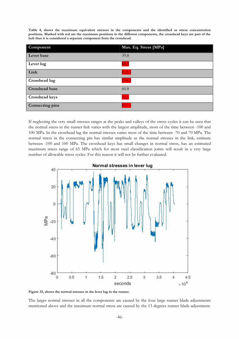
-46-

Table 4, shows the maximum equivalent stresses in the components and the identified as stress concentration positions. Marked with red are the maximum positions in the different components, the crosshead keys are part of the hub thus it is considered a separate component from the crosshead.

Component Max. Eq. Stress [MPa]

Lever base 39.8

Lever lug 88.3

Link 162.3

Crosshead lug 124.4

Crosshead base 60.8

Crosshead keys 45.5

Connecting pins 167.4

If neglecting the very small stresses ranges at the peaks and valleys of the stress cycles it can be seen that

the normal stress in the runner link varies with the largest amplitude, most of the time between -100 and

100 MPa. In the crosshead lug the normal stresses varies most of the time between -70 and 70 MPa. The

normal stress in the connecting pin has similar amplitude as the normal stresses in the link, estimate

between -100 and 100 MPa. The crosshead keys has small changes in normal stress, has an estimated

maximum stress range of 65 MPa which for most steel classification joints will result in a very large

number of allowable stress cycles. For this reason it will not be further evaluated.

Figure 33, shows the normal stresses in the lever lug in the runner.

The larges normal stresses in all the components are caused by the four large runner blade adjustments

mentioned above and the maximum normal stress are caused by the 13 degrees runner blade adjustment.

-47-

In the link the maximum normal stress is over 150 MPa and when the normal stress is reversed it reaches

a lever of about 100 MPa, thus the maximum stress range in the link will be above 250 MPa. In the

crosshead lug the maximum normal stress is around 125 MPa and when it is reversed the normal stress

peaks at 75 MPa, thus the maximum stress range in the cross head lug will be around 200 MPa. The

connecting pin reaches maximum normal stress around 150 MPa and when reversed the normal stress is

about 100 MPa, thus the maximum stress range in the connecting pin will be around 250 MPa.

Since the servomotor force is negative when the runner blade is closing then the normal stresses

calculated are affected by that. The runner link is in tension when the servomotor is applying a negative

force which means that the negative normal forces in the link are tension stresses and the positive are

compressive stresses.

When the servomotor force is opening the runner blade it will cause tension in the lever lug since the link

cause a radial force in the lever out from the center of center of the radius that the lever is rotating

around. This means that the positive normal stresses in the lever lug is in tension and the negative is in

compression.

For the crosshead keys and the connecting pin it is only the normal stress caused by the bending moment

that is considered. The bending will cause a compressive stress at one edge of the component and a

tension stress at the opposite edge, and when the bending moment changes direction the compressive and

tension stress switches edges. Thus, both edges in the component will be subjected to compressive and

tension stresses. This means that one edge of the connecting pin will be subjected to the normal stresses

shown in the figure 37 with the tension stresses represented by the positive values and compressive

stresses by the negative values. For the other edge it will be tension stresses that is negative values and

positive values are representing compressive stresses. This is also true for the crosshead keys.

Figure 34, shows the normal stresses in the runner link.

-48-

Figure 35, shows the normal stresses in the crosshead lug.

Figure 36, shows the normal stresses in the crosshead keys.

-49-

Figure 37, shows the normal stresses in the connecting pin in the runner.

5.7 Life time evaluations

The number of cycles counted with the rain-flow counting method, with a stress range higher than 70

MPa, is shown in figure 38 to 41. Below 70 MPa there are many stress cycles compared to the stress cycles

above 70 MPa, thus if all stresses would be shown in the same histogram then the stress cycles above 70

MPa would not be visible. The stress cycles above 70 MPa has larger contribution than all the stresses

below; hence those below are not displayed in any histograms. The cycles are counted over a 10 hours

period and the reason for not using the whole 11 hours period is that in the beginning of the 11 hours

period there is a startup period that causes stress cycles, which are not considered in this thesis. Only

whole cycles are used to evaluate the accumulative fatigue damage, thus if half cycles are combined into

whole cycles to the extent possible.

As can be seen there are only 3.5 cycles with a stress range over the 70 MPa counted for the lever lug,

which was expected since it was seen in figure 33 that most of the operating time the stress range was well

below 70MPa. In the lever lug there are;

one cycle around 75 MPa

one cycle around 90 MPa

one cycle around 103 MPa

In the runner link there are 18 stress cycles that has a stress range above 70 MPa;

six cycles around 100 MPa

nine cycles around 200 MPa

three cycles around 270 MPa

-50-

In the crosshead lug there are 16 stress cycles that has a stress range above 70 MPa;

four cycles around 80 MPa

nine cycles around 150 MPa

three cycles around 200 MPa

In the runner connecting pin there are 18 stress cycles that has a stress range above 70 MPa;

six cycles around 100 MPa

nine cycles around 200 MPa

three cycles around 250 MPa

Figure 38, shows the counted cycles in the runner lever lug, with a higher stress range than 70 MPa.

-51-

Figure 39, shows the counted cycles in the runner link, with a higher stress range than 70 MPa.

Figure 40, shows the counted cycles in the crosshead lug, with a higher stress range than 70 MPa.

-52-

Figure 41, shows the counted cycles in the runner connecting pin, with a higher stress range than 70 MPa.

The accumulated fatigue damage is calculated according to the Palmgren-Miner rule, where the fatigue

damage for each stress range is summed. The number of allowable cycles is calculated according to

equation (3.17) for the different steel components. The steel in all components in the fatigue calculations

has the same composition except for the crosshead. The crosshead is made of high resistance steel with a

tensile strength of 600 MPa. The other components are made out of forged steel with a tensile strength of

900 MPa. The joint class used is one for non-welded basic material which has been machined, which gives

a FAT-value of 210 MPa.

The results from the fatigue damage calculations are shown in table 5 to 8; only whole cycles have been

used in the calculations and the cycles has been counted over a 10 hour period. The stress ranges shown in

table 5 to 8 are average values (except for the stress ranges below 70 MPa) of the stress ranges within 10

MPa of the values displayed in the tables below. The fatigue damage in the stress range of <70 MPa are

calculated for each cycle in MATLAB and fatigue damage are accumulated into one contribution.

The life time estimations are calculated for two scenarios, in the first scenario it is assumed that the

hydropower station is operated 100% of the annual hours. In the second scenario it is assumed that the

hydropower station will shut down the production during seven hours each night. Thus the hydropower

station is assumed to be in production 71% of the annual hours, which results in about 6205 operating

hours per year.

In table 5 the fatigue damage is calculated for the lever lug and it can be seen that only three whole cycles

was counted above 70 MPa while 623 were counted below. The stress range of the three cycles are quite

low which leads to high number of allowable cycles, thus low accumulated fatigue damage. The lever lug is

estimated to be able to last 34076 years if the turbine is operated as in the 10 hour sequence during 100%

of the annual hours and 48108 years if operating during 71% of the annual hours.

-53-

The fatigue damage in table 6 has been calculated for the runner link; from the normal stress calculation

18 cycles above 70 MPa was counted and 1805 below. The stress range in the link varies the most among

the investigated components, about 200 MPa between the maximum and minimum stress range. At the

stress range of 209.8 MPa the most fatigue damage has been calculated, even if 209.8 MPa is not the

largest stress range for the runner link it is the most frequent stress range of the stress ranges above 70

MPa. The estimated life time of the link was calculated to be 133 years if operated as the 10 hour sequence

100% of the annual hours and 188 years if operated 71% of the annual hours.

Table 7 shows the calculated fatigue damage of the crosshead lug, where 15 cycles has been counted

above 70 MPa and 1447 below. More than half of the stress cycles above 70 MPa has a stress range of

157.5 MPa, thus that stress range is the major contributor to the accumulative fatigue damage. The

estimated life time of the crosshead lug was calculated to be 512 years if operated as the 10 hour sequence

100% of the annual hours and 723 years if operated 71% of the annual hours.

There were 17 stress cycles counted in the runner connecting pin above 70 MPa and 1746 below, the

accumulated fatigue damage is shown in table 8. The stress ranges and distribution is similar to the link,

but with generally smaller stress ranges, this can be seen by comparing figure 39 and 41, the histogram

bars are gathered in similar groups and at similar stress ranges. This leads to similar accumulative fatigue

damage, but slightly lower. The estimated life time of the connecting pin was calculated to be 165 years if

operated as the 10 hours sequence 100% of the annual hours and 233 years if operated 71% of the annual

hours.

Table 5, shows the fatigue damage calculations for the lever lug in the runner.

Lever lug

Stress range

σrd [MPa]

Number of stress cycles

nt

Number of allowable

cycles

Nt [106]

Fatigue damage

nt/Nt

[10-6]

<70 623 - 0.0082

74.7 1 351.17 0.0029

90.4 1 135.30 0.0074

103.6 1 68.44 0.015

Accumulated fatigue damage 0.0335

Estimated life time, 100% of maximum operating hours [years] 34076

Estimated life time, 71% of maximum operating hours [years] 48108

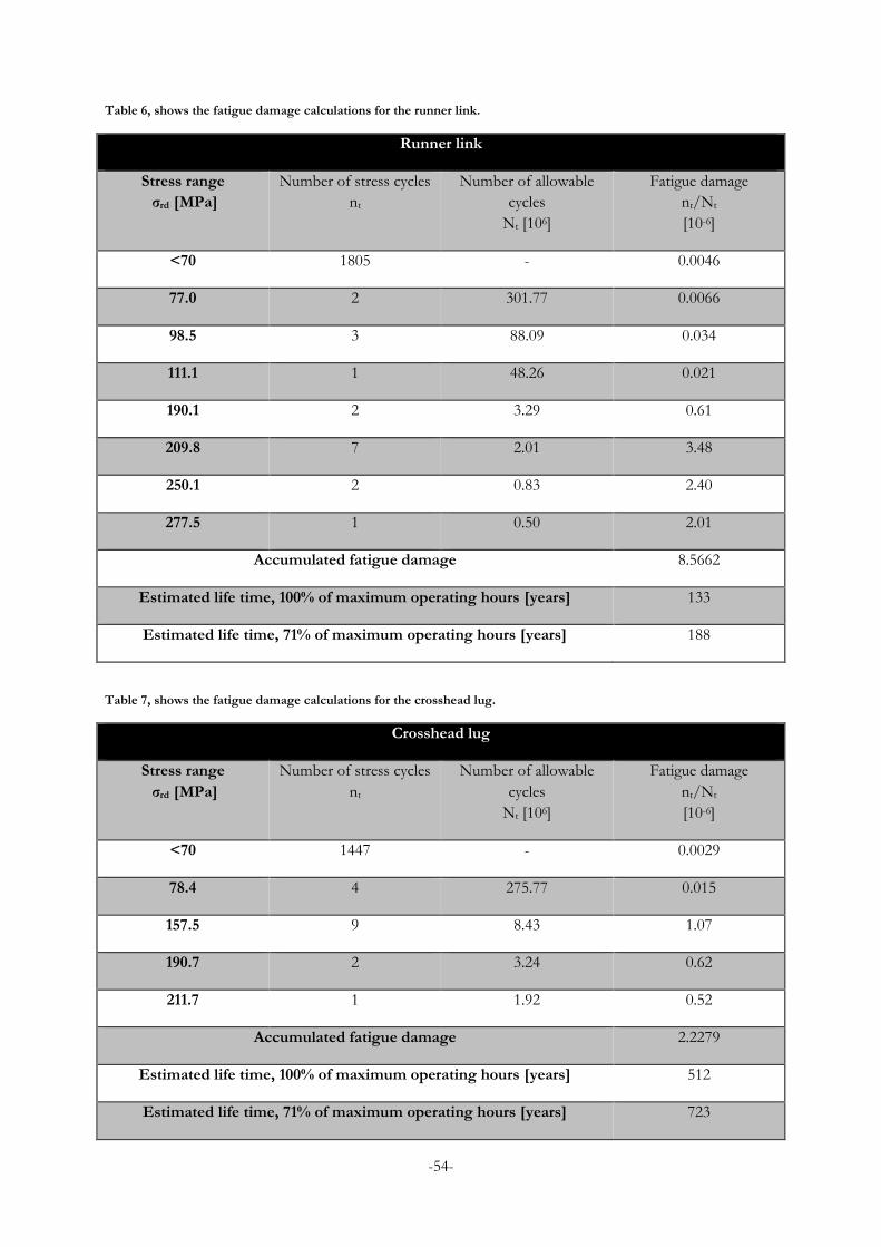
-54-

Table 6, shows the fatigue damage calculations for the runner link.

Runner link

Stress range

σrd [MPa]

Number of stress cycles

nt

Number of allowable

cycles

Nt [106]

Fatigue damage

nt/Nt

[10-6]

<70 1805 - 0.0046

77.0 2 301.77 0.0066

98.5 3 88.09 0.034

111.1 1 48.26 0.021

190.1 2 3.29 0.61

209.8 7 2.01 3.48

250.1 2 0.83 2.40

277.5 1 0.50 2.01

Accumulated fatigue damage 8.5662

Estimated life time, 100% of maximum operating hours [years] 133

Estimated life time, 71% of maximum operating hours [years] 188

Table 7, shows the fatigue damage calculations for the crosshead lug.

Crosshead lug

Stress range

σrd [MPa]

Number of stress cycles

nt

Number of allowable

cycles

Nt [106]

Fatigue damage

nt/Nt

[10-6]

<70 1447 - 0.0029

78.4 4 275.77 0.015

157.5 9 8.43 1.07

190.7 2 3.24 0.62

211.7 1 1.92 0.52

Accumulated fatigue damage 2.2279

Estimated life time, 100% of maximum operating hours [years] 512

Estimated life time, 71% of maximum operating hours [years] 723

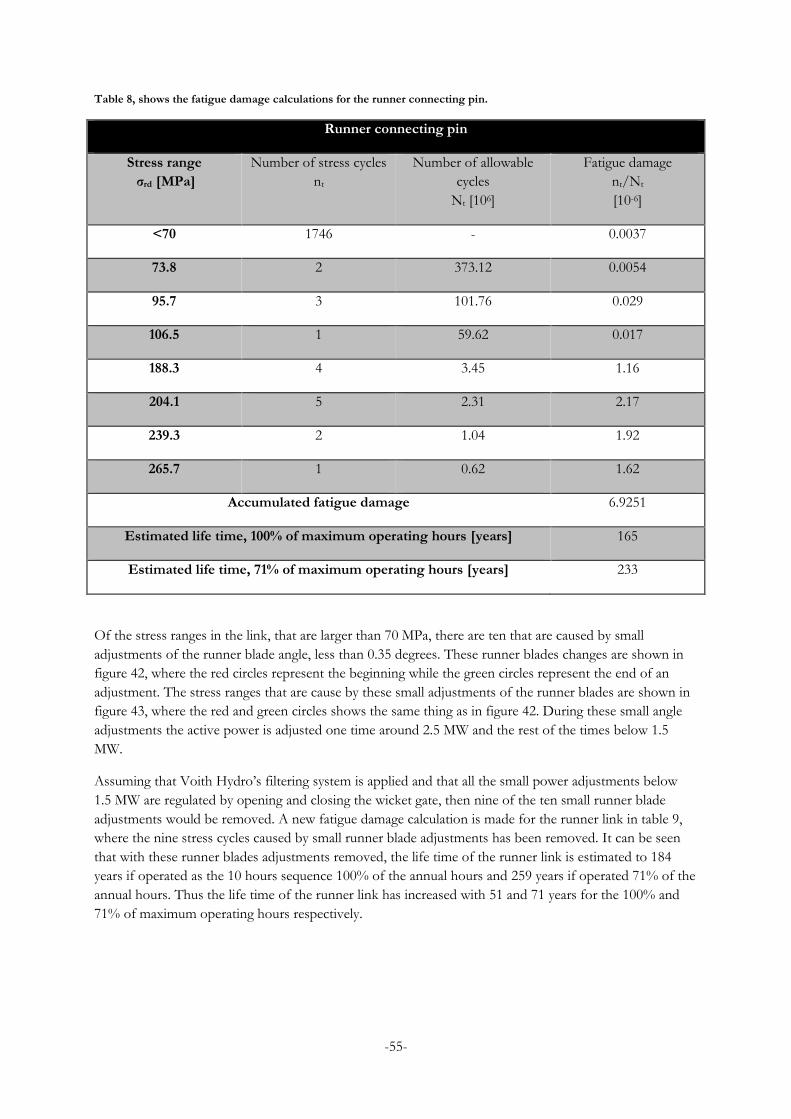
-55-

Table 8, shows the fatigue damage calculations for the runner connecting pin.

Runner connecting pin

Stress range

σrd [MPa]

Number of stress cycles

nt

Number of allowable

cycles

Nt [106]

Fatigue damage

nt/Nt

[10-6]

<70 1746 - 0.0037

73.8 2 373.12 0.0054

95.7 3 101.76 0.029

106.5 1 59.62 0.017

188.3 4 3.45 1.16

204.1 5 2.31 2.17

239.3 2 1.04 1.92

265.7 1 0.62 1.62

Accumulated fatigue damage 6.9251

Estimated life time, 100% of maximum operating hours [years] 165

Estimated life time, 71% of maximum operating hours [years] 233

Of the stress ranges in the link, that are larger than 70 MPa, there are ten that are caused by small

adjustments of the runner blade angle, less than 0.35 degrees. These runner blades changes are shown in

figure 42, where the red circles represent the beginning while the green circles represent the end of an

adjustment. The stress ranges that are cause by these small adjustments of the runner blades are shown in

figure 43, where the red and green circles shows the same thing as in figure 42. During these small angle

adjustments the active power is adjusted one time around 2.5 MW and the rest of the times below 1.5

MW.

Assuming that Voith Hydro’s filtering system is applied and that all the small power adjustments below

1.5 MW are regulated by opening and closing the wicket gate, then nine of the ten small runner blade

adjustments would be removed. A new fatigue damage calculation is made for the runner link in table 9,

where the nine stress cycles caused by small runner blade adjustments has been removed. It can be seen

that with these runner blades adjustments removed, the life time of the runner link is estimated to 184

years if operated as the 10 hours sequence 100% of the annual hours and 259 years if operated 71% of the

annual hours. Thus the life time of the runner link has increased with 51 and 71 years for the 100% and

71% of maximum operating hours respectively.

-56-

Figure 42, shows the runner blade adjustments, where the red and green circles show the beginning and the end respectively of a small runner blade adjustment which causes a stress span above 70 MPa.

Figure 43, shows the stress spans above 70 MPa which are caused by runner blade adjustments smaller than 0.35 degrees. The beginning and end of a stress span is marked with red and green circles respectively.

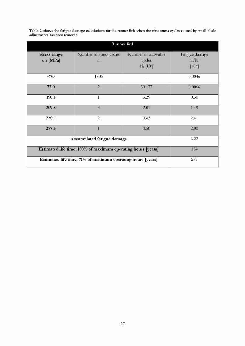
-57-

Table 9, shows the fatigue damage calculations for the runner link when the nine stress cycles caused by small blade adjustments has been removed.

Runner link

Stress range

σrd [MPa]

Number of stress cycles

nt

Number of allowable

cycles

Nt [106]

Fatigue damage

nt/Nt

[10-6]

<70 1805 - 0.0046

77.0 2 301.77 0.0066

190.1 1 3.29 0.30

209.8 3 2.01 1.49

250.1 2 0.83 2.41

277.5 1 0.50 2.00

Accumulated fatigue damage 6.22

Estimated life time, 100% of maximum operating hours [years] 184

Estimated life time, 71% of maximum operating hours [years] 259

-58-

6 Discussion

6.1 The results

6.1.1 Wicket gate

The force needed to adjust the guide vane during frequency regulation is quite small in the context of

fatigue of steel components as seen in section 5.3. Since the components in the wicket gate are designed to

withstand extreme load cases such as a fast stop, the components are generously designed for normal

operation. This means that the components connected between the operating ring and the guide vane

trunnion are considered to be unaffected by frequency regulation.

As mentioned in section 5.5 the maximum equivalent stress in the wicket gate was calculated in the

connecting pin between the servomotor and the operating ring. This is logical since the servomotor force

is applied directly to the connecting pin, but despite this the equivalent stress are not high enough to be

evaluated for accumulative fatigue damage. Hence the connecting pin between the servomotor and the

operating ring is not considered to be affected by frequency regulation.

6.1.2 Runner

The data required was measured around 11 hours between 5.40 am to 4.50 pm on a weekday. For a more

accurate result the sequence should have been longer. In one scenario it is assumed that the hydropower

station is not operating during a seven hours break per day and that these breaks occur during the night,

thus the sequence is a few hours short from the daily production. Further it is assumed that the sequence

could be used to give a relatively good estimation of the fatigue damage during a year since it almost

represents a daily production. In the other scenario it is assumed that the hydropower station is operating

during all of the annual hours.

For the pressure measurements conducted in Jössefors pressure transmitters were used with the accuracy

of ±0.04% of the measurement span, which results in an accuracy of ±0.01 MPa for the set measurement

span. For a servomotor force at 80 kN would deviate with ±0.78 kN which is quite good accuracy. The

accuracy of the pressure measurements that was provided is unknown, but since Voith has used this data

for their own investigations it is considered to have god accuracy as well.

The investigation in the runner was made for the lever, link, connecting pins, crosshead and the crosshead

keys. First the maximum equivalent stress for different sections and parts was calculated to determine

which section of the part that was subjected to the largest stresses. It was decided to neglect the shear

stress when calculating the stress ranges since the contribution of shear stress in the equivalent stress was

negligible. The normal stresses were calculated for the lugs in the lever, link and crosshead, and the normal

stress was calculated in the cross section where the connecting pin changes diameter and at the base of the

crosshead key. From the results of the normal stress calculations it could be seen that calculations of the

fatigue damage of the crosshead keys were not necessary since there were no stress ranges larger than 70

MPa. From the normal stress calculations it could also be seen that the calculations for the lever lug would

be unnecessary, but since there were a few stress ranges larger than 70 MPa the accumulative fatigue

damage was calculated.

In both scenarios the life time estimations were large for both the lever lug and the crosshead lug, so large

that it is theoretically very unlikely that either of these components would fail due to fatigue. However, if

the runner blades are often operated close to the fully opened position, then the accumulative fatigue

damage would increase and the life time of the lug would decrease. The runner blades are operated close

to fully opened position during about one hour and during that hour all three stress ranges above 70 MPa

is measured. Thus if the hydropower station would be operated like that hour for the whole year the life

-59-

time of the lever lug would decrease to about 4500 years which is a very large decrease of life time.

However, the estimated life time is still very large and theoretically it is not likely to fail due to fatigue.

According to the life time estimations, of the investigated components it is the link and the connecting pin

that are most likely to fail due to fatigue. If the hydropower station would be operated during 100% of the

annual hours then the life time of the link and connecting pin would be 133 and 165 years respectively. If

the hydropower station would be operated during 71% of the annual hours then the link and connecting

pin would have an estimated life time of 188 and 233 years respectively. When designing a turbine it is

common to design it to last at least 40 years, from that point of view the components will have safety

factor of more than 3 and 4 respectively. Even if the life time estimation shows that the components are

designed against a theoretical fatigue failure a component can still fail due to fatigue. In this thesis the life

time estimations are assuming that the hydropower station is operated accordingly to the 10 hour

sequence, but if the operators would run the station with larger and/or more frequent load variations then

the risk for fatigue would increase.

If the filtering system developed by Voith is applied to reduce the number of movements of the runner

blades and set to keep the runner blade at a constant position for blade adjustments smaller than 0.35

degrees then half of the stress cycles above 70 MPa in the link would be removed. This would result in an

increased life time of 38% in both scenarios, but it is a trade off with decreased turbine efficiency and

increased stresses in the wicket gate. The filter that suppresses the noise in the frequency would reduce the

amount of stress cycles as well since lots of the fluctuations in the frequency signal has been removed, but

without the logged frequency it is impossible to know how many and which stress cycles that would be

removed. The 38% increased life time will be higher if the effect of first filter could be determined.

Increased stresses in the wicket gate are preferable to increased stresses in the runner, since the force to

adjust one guide vane is less than to adjust one runner blade. If a component would fail then it will be

easier and less expensive to replace a component in the wicket gate compared to one in the runner,

especially if the runner has the servomotor located upstream of the runner blades. The replacement of a

component in the wicket gate can be done while the turbine has been stopped, while a replacement of a

component in the runner also requires the water outside and water/oil inside of the turbine to be

evacuated, at least. It might even be necessary to lift up the turbine to gain access.

6.2 Limitations of the investigation

The measurement sequence of the pressure in the wicket gate servomotor was less than one hour, which

is considered quite small and it was carried out around 11 pm. Since it is a short period of time it is

difficult to claim that this sequence would be representative for a life time of operation, especially when it

was measured at 11 pm a weekday. Usually from 11 pm to 6 am the total production and consumption in

the Swedish grid is relatively constant during a weekday. Hence it would have been better with a measured

sequence of at least 24 hours during a weekday so that the sequence would contain the production and

consumption patterns of a whole day.

The estimated life time calculations has only taken the load changes during normal operation into

consideration for both scenarios, but accumulative fatigue damage is also caused by other types of

loadings as well. In the scenario where the hydropower station is shutting down during the night, the start

and stops cycles will also contribute to the accumulative fatigue damage. In the other scenario no start and

stops are considered but in a real case it is likely that the hydropower station has to shut down some times,

for example, to perform maintenance or because of the amount of water in the reservoirs. For a more

accurate estimation, all types of loadings that contribute to the accumulative fatigue damage has to be

considered, even those that only occurs a few times during the life time of the turbine if the stress ranges

are large.

-60-

In the regulating mechanism no losses due to friction has been taken into account, when the force is

transferred between the different components in the regulation mechanism some part will be lost in

between two components. Thus the largest difference would be in the lever since it is the last component

that the servomotor force is transferred to.

The methods used to calculate the normal and shear stresses are calculated from the nominal stresses

which are based upon simple or common cross sections. For some of the components the cross sections

were assumed to have a simpler geometry so that the nominal stress could be calculated. The lever in the

wicket gate was assumed to have a U-shaped cross section with sharp edges instead rounded edges and

the crosshead lug was assumed to be a simple lug with the same width on both sides of the hole which is

not the real case. These simplifications will affect the nominal stresses calculated in the components, how

much is hard to determine, but since the difference between the simplified and real shapes are quite small

it is assumed that the error in the calculated nominal stresses will be quite small as well.

The same calculations made in this thesis could have been done with FEM which probably would have

given a more accurate result. One of the advantages with FEM compared to the simplified model used is

that the whole geometry can be evaluated and no simplification of the geometries has to be made. In FEM

the accuracy can be changes by applying a finer or coarser mesh. The exact location of the stress

concentrations will be shown in in FEM while in the model used it is only estimated where the stress

concentrations are located.

The guideline used to calculate the number of allowable cycles at a certain stress range is focusing on

components manufactured from steel sheets, thus the material joint used is for a steel sheet that has been

machined. Since the components are casted and then machined the material joint used might result in a

different S-N curve then the S-N curve for the different components. It is assumed that the difference can

be neglected since the component has been machined which would give the same surface roughness of

the component regardless if it has been casted or made out of steel sheets.

The results calculated with the provided data from Voith cannot be applied to the runner in Jössefors.

First of all the design of the runner are different, Jössefors has the servomotor upstream of the runner

blades and the regulating mechanism is not the same. Instead of links connecting the crosshead to the

lever it has a cube which is mounted in a horizontal track in the crosshead, thus when the crosshead is

moving in the vertical direction the cube can move the lever in vertical direction and follow the lever in

horizontal direction. The diameter of the runner is about 3 m longer than the runner in Jössefors and the

rated head is about 15 m higher than the rated head in Jössefors which means that the loading condition

upon the runner blades is quite different than the loading condition in Jössefors.

-61-

7 Conclusions

From the calculations it could be determined that the stresses in the wicket gate are smaller than the

stresses in the runner. However, the connecting pin between the servomotor and operating ring were

subjected too much larger stresses than any of the other components in the wicket gate, but the stresses

were still not large enough to be considered a component with risk of fatigue failure.

In the runner the largest stresses were calculated in the link and the connecting pin, but the risk of fatigue

failure was considered small. If the turbine would be operated according to the 10 hour sequence during

all the hours of the year the link and connecting pin would have a theoretical life time of 133 and 165

years respectively. It the turbine instead would be operated during 71% of the annual hours the theoretical

life time of the link and connecting pin would be 188 and 233 years respectively. Usually components are

designed to last at least 40 years, thus the link and connecting pin would have a safety factor larger than 3

and 4 respectively.

If the Voith developed filtering system would be applied the theoretically life time would be further

increased for the components. If all runner blade adjustments smaller than 0.35 degrees with a change in

active power less than 1.5 MW would be removed by the second filter then half of the stress cycles with a

stress span larger than 70 MPa in the link would have been removed. This measure would increase the

theoretically life time of the link to 184 years in the scenario where all the annual hours are used for

operation and 259 years in the scenario where 71% of the annual hours are used for operation. Probably a

lot of the smaller stress cycles could be removed by the first as well as the second filter, but that need

further investigation.

For older Kaplan turbines that would be used for frequency regulation are recommended to apply Voiths

filtering system or regulate the number of adjustments of the runner blade angle using a dead-band. The

older Kaplan turbines might not be designed for frequency regulation, thus it might be a good idea to

reduce the number of stress cycles. It could be a good idea to reduce the number of stress cycles in newer

Kaplan turbines as well since fatigue failure can occur within a life time even if it in theory should not. To

reduce the stress cycles is an extra safety factor against fatigue failure. It is also good to reduce the wear of

the bushings and bearings, which if old and worn could cause failure or increase the servomotor force,

needed which increases the risk for fatigue failure.

It could be interesting to investigate the tradeoff between efficiency and wear if the number of

movements in the runner would be decreased. It would also be interesting to see how much this would

affect the stresses in the wicket gate, if the servomotor force or/and the number of cycles increases it

might be interesting to investigate the connecting pin between the servomotor and operating ring.

-62-

Bibliography

[1] W. Forsström, "Utredning av frekvensregleringens påverkan på mekanisk utrustning i en

kaplanturbin," Uppsala Universitet, Uppsala, 2015.

[2] J. Hölcke, "Hydrauliska Strömningsmaskiner," Stockholm, 2002.

[3] R. C. Dorf, The Engineering Handbook – Second Edition, CRC Press LLC, 2005.

[4] A. Kjølle, HYDROPOWER IN NORWAY; Mechanical Equipment, Trondheim: Norwegian

University of Science and Technology, 2001.

[5] G. (. Grilli and P.Eng, "Hydraulic Unit Governor Upgrading Guide," CEATI INTERNATIONAL

Inc., Montreal, 2011.

[6] F. Armand, G. S. Bruno, M. Laguna and C. Penche, "Guide on How to Develop a Small Hydropower

Plant," European Small Hydropower Association, 2004.

[7] M. G. Rabie, Fluid Power Engineering, McGraw-Hill Professional Publishing, 2009.

[8] R. Falkenhem, "Typlösningar för komponenter," Kvaerner Turbin AB, 1991.

[9] J. Ukonsaari, "Erfarenheter med miljöanpassade Kaplanlöphjul," Elforsk, 2012.

[10] Y. Luo, Z. Wang, J. Zeng and J. Lin, "Fatigue of piston rod caused by unsteady, unbalanced,

unsynchronized," Engineering Failure Analysis, vol. 17, no. 1, pp. 192-199, 2010.

[11] L. Söder and M. Amelin, "Effektiv drift och planering av kraftsystem," Royal Institute of Technology,

Stockholm, 2011.

[12] Svenska Kraftnät, "Regler för upphandling och redovisning av FCR," Svenska Kraftnät, Sundbyberg,

2015.

[13] Statens energimyndighet, "Vad avgör ett vattenkraftverks betydelse för elsystemet," Statens

energimyndighet, 2014.

[14] B. G. Liptak, Instrument Engineers' Handbook, Fourth Edition, Volume Two: Process Control and

Optimization, CRC Press, 2005.

[15] S. Brausewetter and T. Kächele, "New frequency sensitive control mode for Kaplan and bulb

turbines," Heidenheim.

[16] W. D. Pilkey and D. F. Pilkey, Peterson's Stress Concentration Factors, Hoboken: John Wiley &

Sons, Inc., 2008.

[17] A. P. Boresi, O. M. Sidebottom, F. B. Seely and J. O. Smith, Advanced Mechanics of Materials, New

York: John Wiley & Sons, Inc., 1978.

[18] T. Dahlberg, Teknisk hållfasthetslära, Lund: Studentlitteratur, 2001.

[19] J. L. Otegui, Failure Analysis; Fundamentals and Applications in Mechanical Components,

Switzerland: Springer International Publishing, 2014.

[20] F. Campbell, Elements of Metallurgy and Engineering Alloys, ASM International, 2008.

[21] SSAB, Plåthandboken; Att konstruera och tillverka i höghållfast stål, SSAB, 2011.

-63-