A Fast and Parametric Torque Distribution Strategy for ... · PDF fileof energy dissipations...

http://curve.coventry.ac.uk/open

A Fast and Parametric Torque Distribution Strategy for Four-Wheel-Drive Energy-Efficient Electric Vehicles Kikuchi, H. , Reiman, A. , Nyoni, J. , Lloyd, K. , Savage, R. , Wotherspoon, T. , Berry, L. , Snead, D. and Cree, I. A. Published PDF deposited in Curve March 2016 Original citation: Moradinegade Dizqah, A. , Lenzo, B. , Sorniotti, A. , Gruber, P. , Fallah, S. and De Smet, J. (Forthcoming) A Fast and Parametric Torque Distribution Strategy for Four-Wheel-Drive Energy-Efficient Electric Vehicles. IEEE Transactions on Industrial Electronics, volume (In Press) Publisher: IEEE Sponsored by: IEEE Industrial Electronics Society Published under Gold Open Access (c) 2016 IEEE. Personal use of this material is permitted. Permission from IEEE must be obtained for all other users, including reprinting/ republishing this material for advertising or promotional purposes, creating new collective works for resale or redistribution to servers or lists, or reuse of any copyrighted components of this work in other works. Copyright © and Moral Rights are retained by the author(s) and/ or other copyright owners. A copy can be downloaded for personal non-commercial research or study, without prior permission or charge. This item cannot be reproduced or quoted extensively from without first obtaining permission in writing from the copyright holder(s). The content must not be changed in any way or sold commercially in any format or medium without the formal permission of the copyright holders.

CURVE is the Institutional Repository for Coventry University

http://curve.coventry.ac.uk/open

0278-0046 (c) 2015 IEEE. Translations and content mining are permitted for academic research only. Personal use is also permitted, but republication/redistribution requires IEEE permission. Seehttp://www.ieee.org/publications_standards/publications/rights/index.html for more information.

This article has been accepted for publication in a future issue of this journal, but has not been fully edited. Content may change prior to final publication. Citation information: DOI 10.1109/TIE.2016.2540584, IEEETransactions on Industrial Electronics

IEEE TRANSACTIONS ON INDUSTRIAL ELECTRONICS

Abstract — Electric vehicles with four individually controlled drivetrains are over-actuated systems and therefore the total wheel torque and yaw moment demands can be realized through an infinite number of feasible wheel torque combinations. Hence, an energy-efficient torque distribution among the four drivetrains is crucial for reducing the drivetrain power losses and therefore extending driving range. In this paper, the optimal torque distribution is formulated as the solution of a parametric optimization problem, depending on vehicle speed. An analytical solution is provided for the case of equal drivetrains, under the experimentally confirmed hypothesis that the drivetrain power losses are strictly monotonically increasing with the torque demand. The easily implementable and computationally fast wheel torque distribution algorithm is validated by simulations and experiments on an electric vehicle demonstrator, along driving cycles and cornering maneuvers. The results show considerable energy savings compared to alternative torque distribution strategies.

Index Terms — Electric vehicle; torque distribution;

control allocation; power loss; experiments.

I. INTRODUCTION

ne of the main obstacles to the success of electric

vehicles (EVs) in the automotive market is their limited

driving range. This issue is addressed by research in novel

battery technologies to increase energy density and, hence, to

provide viable/lightweight high-capacity energy storage

systems. On the other hand, energy management systems are

conceived to improve vehicle efficiency through advanced

control of the drivetrains and ancillaries. In particular, EVs

Manuscript received August 10, 2015; revised October 18, 2015

and December 1, 2015; accepted February 2, 2016. This work was supported by the European Union Seventh Framework Programme FP7/2007-2013 under the iCOMPOSE project (grant agreement no. 608897).

A. M. Dizqah was with the Centre for Automotive Engineering, University of Surrey, Guildford, GU2 7XH, UK. He is now with the Centre for Mobility and Transport, Coventry University, CV1 5FB, UK. B. Lenzo, A. Sorniotti, P. Gruber, S. Fallah are with the Centre for Automotive Engineering, University of Surrey, Guildford, GU2 7XH, UK. J. De Smet is with Flanders MAKE, 3920 Lommel, Belgium.

with multiple drivetrains allow the implementation of control

functions, such as front-to-rear and left-to-right torque-

vectoring, which improve active safety and drivability, and

contribute to the attractiveness of EV technology [1-2]. Owing

to the use of multiple motors an actuation redundancy is

obtained – that is, the desired vehicle behavior corresponding

to the driver’s inputs at the accelerator/brake pedal and/or

steering wheel can be realized through an infinite number of

feasible wheel torque distributions. For the range of feasible

torque distributions, this paper presents a novel solution

providing maximum energy efficiency.

The two major sources of power loss in EVs are the

drivetrains and the tires. The drivetrain power losses include

the contributions of the drives, electric motors and

transmissions (where present). Tire contributions relate to

rolling resistance, longitudinal slip and lateral slip, with the

latter two being relevant only at significant acceleration levels

[3].

Prior research (e.g., [4-8]) indicates that the power losses

can be reduced by specific torque distribution algorithms, also

called control allocation (CA) strategies. For instance, [4,9]

present CA strategies minimizing energy dissipation due to

tire slip. Although effective, the practical implementation of

these strategies requires some form of continuous estimation

of the longitudinal and lateral slip velocities of each tire,

which is beyond the capability of existing state estimators in

normal driving conditions. In [5-7] and [10-12] the reduction

of energy dissipations within the electric motor drives is

examined. The presented strategies are mainly based on

experimentally measured efficiency maps of electric motors.

In particular, [5] carries out an off-line calculation of the

optimal wheel torques, but without analyzing the resulting

wheel torque distribution as a function of the input parameters,

i.e., wheel torque demand and vehicle speed. The results in [5]

imply that the optimal solution is either to only use a single

axle or to evenly distribute the torque among the front and rear

drives of the EV. Moreover, the CA strategies in [6,12-13] are

shown to be more efficient than the simple even torque

distribution among the front and rear axles. However, the

influence of vehicle speed (𝑉) on the optimal solution is not

directly taken into account.

A Fast and Parametric Torque Distribution Strategy for Four-Wheel-Drive Energy

Efficient Electric Vehicles

Arash M. Dizqah, Member, IEEE, Basilio Lenzo, Member, IEEE, Aldo Sorniotti, Member, IEEE, Patrick Gruber, Saber Fallah, Jasper De Smet

O




Fig. 1. The vehicle dynamics control structure

The effect of speed variation is investigated in [7] but it is not

formulated. [10] discusses the change of the optimal

distribution ratio as a function of longitudinal acceleration.

The problem formulation is novel with results indicating small

variations of the optimal distribution ratio over the achievable

acceleration range. According to the results in [10], the vehicle

never operates in the ‘single-axle’ mode, which is shown in

[5,8] to be the optimal solution for small torque demands.

Also, [10] only considers straight line driving. [11] presents a

CA strategy that is based on a simplified piecewise-linear

efficiency map of the brushless DC motors. An algorithm,

based on Karush-Kuhn-Tucker (KKT) conditions of

optimality, finds global solutions of the CA problem for non-

monotonically increasing drivetrain power loss curves. The

corresponding non-convex optimization problem is translated

into a number of equivalent eigenvalue problems. [14-15]

propose high-level controllers aimed at achieving the

reference cornering response, coupled with CA algorithms to

improve vehicle stability (e.g., based on tire workload

reduction). However, [4] shows that such strategies can be far

from optimal in terms of energy efficiency.

In summary, an extensive literature deals with the subject of

CA strategies for four-wheel-drive EVs. Many of the proposed

algorithms are designed for reduced tire slip variance among

the wheels. The papers dealing with drivetrain energy

efficiency either do not discuss the resultant wheel torque

distribution maps, or they present very complicated algorithms

(such as multi-parametric non-convex optimization, [16-17]),

which are unlikely to be directly implemented on production

vehicles. As a consequence, there is a clear need for simple,

computationally efficient, easily-tunable and effective

solutions of the CA problem aimed at drivetrain energy

efficiency. The gap is addressed by this paper, including the

following novel contributions:

i) The analytical solution of the CA problem maximizing

energy efficiency, under the hypothesis of strictly

monotonically increasing drivetrain power losses with

wheel torque demand. The optimal solution, obtained for

the case of equal drivetrains, is parameterized as a function

of 𝑉;

ii) A fast and easily implementable torque distribution

strategy maximizing energy efficiency, based on the

proposed analytical solution in i);

iii) The simulation-based and experimental validation of the

energy benefits of the CA algorithm in cornering

conditions and along driving cycles.

The remainder of the paper is organized in four sections (II

to V). Section II formulates the energy-efficient CA problem

as a multi-parametric non-convex optimization. Section III

provides the theoretical background required to design the

proposed fast CA for EVs. The performance of the CA

strategy is verified in Section IV through computer

simulations with a vehicle dynamics model and experiments

on an electric Range Rover Evoque demonstrator vehicle.

Finally, the conclusions are provided in Section V.

II. PROBLEM STATEMENT AND FORMULATION

A. Problem statement

Fig. 1 shows the simplified vehicle control structure. The

reference generator outputs the reference yaw rate, 𝑟𝑟𝑒𝑓 , and

traction/braking force, 𝐹𝑟𝑒𝑓, starting from the steering wheel

angle (𝛿), accelerator and brake pedal positions (respectively

𝐴𝑃𝑃 and 𝐵𝑃𝑃), and longitudinal vehicle speed and

acceleration (respectively 𝑉 and 𝑎𝑥). The high-level controller

calculates the corrected longitudinal force reference, �̃�𝑟𝑒𝑓 (i.e.,

𝐹𝑟𝑒𝑓 from the reference generator is reduced in extreme

cornering conditions), and the yaw moment reference, ∆𝑀𝑟𝑒𝑓 ,

e.g., based on the combination of feedforward and feedback

control of vehicle yaw rate, 𝑟. The proposed CA strategy must minimize the drivetrain

power loss while maintaining �̃�𝑟𝑒𝑓 (each drivetrain can operate

in either traction or regeneration) and ∆𝑀𝑟𝑒𝑓. As the drivetrain

power losses are functions of 𝑉, the CA strategy includes 𝑉 as

a parameter.

The CA problem is formulated as a static optimization or

quasi-dynamic optimization [18-20] to be solved at each time

step for the values of �̃�𝑟𝑒𝑓 and ∆𝑀𝑟𝑒𝑓 calculated by the high-

level controller, and the estimated 𝑉 (Fig. 1). The CA strategy

could be integrated into the high-level controller, thus giving

origin to a single multiple-input multiple-output controller. On

the other hand, the separation among the high-level controller

and the CA strategy (Fig. 1) has advantages, such as ease of

considering actuator limitations [21] and flexibility with

respect to the drivetrain configuration. The following

subsection will formulate the CA problem mathematically,

under Assumptions 1 and 2.




3

Assumption 1: The case study EV includes four identical

electric drivetrains with equal power loss characteristics – i.e.,

the electric machines and their power electronics, single-speed

gearboxes, constant-velocity joints and wheels are the same on

each vehicle corner.

Assumption 2: The drivetrain power loss characteristic on each

vehicle corner, 𝑃𝑙𝑜𝑠𝑠(𝜏𝑤 , 𝑉), is positive and strictly

monotonically increasing as a function of wheel torque

demand, 𝜏𝑤. This means that 𝑃𝑙𝑜𝑠𝑠(𝜏𝑤 , 𝑉) > 0 and

𝜕𝑃𝑙𝑜𝑠𝑠(𝜏𝑤 , 𝑉)/𝜕𝜏𝑤 > 0.

The results presented in the next paragraphs can also be

applied (with specific re-arrangements) to the simplified case

of a four-wheel-drive EV with a single drivetrain per axle.

B. Mathematical formulation

The proposed optimal CA problem for small steering angles is

formulated as follows:

{𝜏𝑤}∗(�̃�𝑟𝑒𝑓 , Δ𝑀𝑟𝑒𝑓 , 𝑉)

= arg min𝜏𝑤𝑖,𝑡 ,𝜏𝑤𝑖,𝑔

𝐽 (𝜏𝑤𝑖,𝑡 , 𝜏𝑤𝑖,𝑔 , 𝑉)

≔∑[𝑠𝑖𝑔𝑛(𝜏𝑤𝑖,𝑡)𝑃𝑖,𝑡(𝜏𝑤𝑖,𝑡 , 𝑉)

4

𝑖=1

− 𝑠𝑖𝑔𝑛 (𝜏𝑤𝑖,𝑔) 𝑃𝑖,𝑔 (𝜏𝑤𝑖,𝑔 , 𝑉)]

𝑠. 𝑡. ∑ (𝜏𝑤𝑖,𝑡 − 𝜏𝑤𝑖,𝑔) = �̃�𝑟𝑒𝑓𝑅4𝑖=1

𝑑𝑓 (𝜏𝑤2,𝑡 + 𝜏𝑤1,𝑔 − 𝜏𝑤1,𝑡 − 𝜏𝑤2,𝑔) +

𝑑𝑟 (𝜏𝑤4,𝑡 + 𝜏𝑤3,𝑔 − 𝜏𝑤3,𝑡 − 𝜏𝑤4,𝑔) = ∆𝑀𝑟𝑒𝑓𝑅

0 ≤ 𝑉 ≤ 𝑉𝑚𝑎𝑥

0 ≤ 𝜏𝑤𝑖,𝑡 ≤ 𝜏𝑤,𝑚𝑎𝑥,𝑖,𝑡

0 ≤ 𝜏𝑤𝑖,𝑔 ≤ 𝜏𝑤,𝑚𝑎𝑥,𝑖,𝑔

𝜏𝑤𝑖,𝑡𝜏𝑤𝑖,𝑔 = 0; 𝑖 = 1,2,3,4

(1)

In the notation of the paper {𝜏𝑤}∗ is the vector with the

optimal values of the torques, which has different dimension

depending on the specific formulations of the optimization

problem presented in the manuscript. 𝜏𝑤𝑖,𝑡 and 𝜏𝑤𝑖,𝑔 are the

traction and regeneration torque demands at the different

wheels (numbered as in Fig. 1). 𝑅 is the tire radius. 𝑑𝑓 and 𝑑𝑟

are the front and rear half-tracks. 𝜏𝑤,𝑚𝑎𝑥,𝑖,𝑡 and 𝜏𝑤,𝑚𝑎𝑥,𝑖,𝑔 are

the minimum between the torque available at the drivetrain in

traction, 𝜏𝑤,𝑚𝑎𝑥,𝑡(𝑉), or regeneration, 𝜏𝑤,𝑚𝑎𝑥,𝑔(𝑉), and the

transmissible torque at the tire-road contact, 𝜇𝑥 𝐹𝑧,𝑖𝑅, being 𝜇𝑥

the estimated tire-road friction coefficient (in longitudinal

direction) and 𝐹𝑧,𝑖 the estimated vertical load at the wheel 𝑖.

The first and second constraints in (1) have a clear physical

meaning in terms of vehicle dynamics: they require that the

torques applied to the wheels generate, respectively, the

corrected longitudinal force reference, �̃�𝑟𝑒𝑓, and the reference

yaw moment, ∆𝑀𝑟𝑒𝑓, of the torque-vectoring controller.

∆𝑀𝑟𝑒𝑓 is actuated through different wheel torques on the two

sides of the vehicle.

In the hypothesis of low load transfers, Problem (1) has

three parameters: i) �̃�𝑟𝑒𝑓; ii) ∆𝑀𝑟𝑒𝑓 and iii) 𝑉. The problem is

non-convex due to the complementarity constraints and non-

convexities in the power loss characteristics of the electric

machines and mechanical transmission systems. The

complementarity constraints 𝜏𝑤𝑖,𝑡𝜏𝑤𝑖,𝑔 = 0 specify that at each

instant each wheel can only operate in traction or regeneration,

For the same reason the 𝑠𝑖𝑔𝑛 function in (1) allows to take

only either 𝑃𝑖,𝑡 or 𝑃𝑖,𝑔 (note that 𝑠𝑖𝑔𝑛(0) = 0). 𝑃𝑖,𝑡 and 𝑃𝑖,𝑔

are, respectively, the drawn and regenerated electrical powers

at the wheel 𝑖, given by:

𝑃𝑖,𝑡 = 𝜏𝑤𝑖,𝑡𝑉

𝑅+ 𝑃𝑙𝑜𝑠𝑠,𝑡(𝜏𝑤𝑖,𝑡 , 𝑉); 𝑖 = 1,2,3,4

(2) 𝑃𝑖,𝑔 = 𝜏𝑤𝑖,𝑔

𝑉

𝑅− 𝑃𝑙𝑜𝑠𝑠,𝑔 (𝜏𝑤𝑖,𝑔 , 𝑉) ; 𝑖 = 1,2,3,4

where the first term on the right-hand side is the mechanical

power at the wheel and the second term is the power loss. The

power losses of all vehicle corners are modeled with the same

functions, 𝑃𝑙𝑜𝑠𝑠,𝑡/𝑔 (the subscripts indicate traction and

regeneration, respectively), obtained by fitting the

experimental measurements on the drivetrains to a

mathematical expression (Assumption 1). In general, the

power loss characteristics are different from zero at zero wheel

torque demand. This is the reason for the 𝑠𝑖𝑔𝑛 function in (1).

By replacing (2) into the cost function 𝐽 (𝜏𝑤𝑖,𝑡 , 𝜏𝑤𝑖,𝑔 , 𝑉) of

(1), 𝐽 is reformulated as:

𝐽 (𝜏𝑤𝑖,𝑡 , 𝜏𝑤𝑖,𝑔 , 𝑉) =𝑉

𝑅(∑ (𝜏𝑤𝑖,𝑡 − 𝜏𝑤𝑖,𝑔)4𝑖=1

⏞

�̃�𝑟𝑒𝑓 𝑅

) +

∑ [𝑠𝑖𝑔𝑛(𝜏𝑤𝑖,𝑡)𝑃𝑙𝑜𝑠𝑠,𝑡(𝜏𝑤𝑖,𝑡 , 𝑉) +4𝑖=1

𝑠𝑖𝑔𝑛 (𝜏𝑤𝑖,𝑔) 𝑃𝑙𝑜𝑠𝑠,𝑔 (𝜏𝑤𝑖,𝑔 , 𝑉)]

(3)

where the first term on the right-hand side is the overall

mechanical power at the wheels and the second term is the

overall power loss.

The term (𝑉/𝑅)�̃�𝑟𝑒𝑓𝑅 is constant for given values of the

parameters. Hence, the cost function can be reduced to:

𝐽 (𝜏𝑤𝑖,𝑡 , 𝜏𝑤𝑖,𝑔 , 𝑉) = ∑ [𝑠𝑖𝑔𝑛(𝜏𝑤𝑖,𝑡)𝑃𝑙𝑜𝑠𝑠,𝑡(𝜏𝑤𝑖,𝑡 , 𝑉) +4𝑖=1

𝑠𝑖𝑔𝑛 (𝜏𝑤𝑖,𝑔) 𝑃𝑙𝑜𝑠𝑠,𝑔 (𝜏𝑤𝑖,𝑔 , 𝑉)] (4)

(4) assumes that the vehicle operates with limited yaw rate and

limited relative slip among the wheels, which means that 𝑉

can be used as the speed of each vehicle corner.

In summary, (1) is a multi-parametric Non-Linear

Programming (mp-NLP) problem [22-23], with the following

general formulation:

𝑧(𝜃) = min𝑥∈𝑋

𝐽 (𝑥, 𝜃)

𝑠. 𝑡. 𝐺(𝑥, 𝜃) ≤ 0; 𝐻(𝑥, 𝜃) = 0; 𝜃 ∈ Θ

(5)

where 𝜃 = [�̃�𝑟𝑒𝑓 , ∆𝑀𝑟𝑒𝑓 , 𝑉]𝑇is the parameter vector, and 𝐺

and 𝐻 represent the inequality and equality constraints.




4

III. CONTROLLER DESIGN

Lemma 1: Problem (1) has only one solution for each side of

the vehicle, assuming 𝑑 = 𝑑𝑓 = 𝑑𝑟:

𝜏𝑤,𝑙∗ = 0.5 (�̃�𝑟𝑒𝑓 −

∆𝑀𝑟𝑒𝑓

𝑑)𝑅;

𝜏𝑤,𝑟∗ = 0.5 (�̃�𝑟𝑒𝑓 +

∆𝑀𝑟𝑒𝑓

𝑑) 𝑅;

−𝜏𝑤,𝑚𝑎𝑥,𝑙,𝑔 ≤ 𝜏𝑤,𝑙∗ ≤ 𝜏𝑤,𝑚𝑎𝑥,𝑙,𝑡;

−𝜏𝑤,𝑚𝑎𝑥,𝑟,𝑔 ≤ 𝜏𝑤,𝑟∗ ≤ 𝜏𝑤,𝑚𝑎𝑥,𝑟,𝑡

(6)

where 𝜏𝑤,𝑙∗ and 𝜏𝑤,𝑟

∗ are, respectively, the optimal wheel torque

demands of the left- and right-hand sides of the vehicle, with

𝜏𝑤,𝑚𝑎𝑥,𝑙,𝑡/𝑔 = 𝜏𝑤,𝑚𝑎𝑥,1,𝑡/𝑔 + 𝜏𝑤,𝑚𝑎𝑥,3,𝑡/𝑔 and 𝜏𝑤,𝑚𝑎𝑥,𝑟,𝑡/𝑔 =

𝜏𝑤,𝑚𝑎𝑥,2,𝑡/𝑔 + 𝜏𝑤,𝑚𝑎𝑥,4,𝑡/𝑔 (the subscripts ‘𝑡’ and ‘𝑔’ indicate

traction and regeneration, respectively).

Proof: From the vehicle schematic in Fig. 1:

𝜏𝑤,𝑙 = 𝜏𝑤1,𝑡 + 𝜏𝑤3,𝑡 − 𝜏𝑤1,𝑔 − 𝜏𝑤3,𝑔

𝜏𝑤,𝑟 = 𝜏𝑤2,𝑡 + 𝜏𝑤4,𝑡 − 𝜏𝑤2,𝑔 − 𝜏𝑤4,𝑔 (7)

where 𝜏𝑤,𝑙 and 𝜏𝑤,𝑟 are, respectively, the wheel torque

demands of the left- and right-hand sides of the vehicle.

By replacing (4) and (7) into (1), Problem (1) becomes:

{𝜏𝑤}∗(�̃�𝑟𝑒𝑓 , ∆𝑀𝑟𝑒𝑓 , 𝑉)

= arg min𝜏𝑤,𝑙,𝜏𝑤,𝑟

𝐽(𝜏𝑤,𝑙 , 𝜏𝑤,𝑟 , 𝑉)

∶= 𝑃𝑙𝑜𝑠𝑠𝑙(𝜏𝑤,𝑙 , 𝑉) + 𝑃𝑙𝑜𝑠𝑠𝑟(𝜏𝑤,𝑟 , 𝑉)

𝑠. 𝑡. 𝜏𝑤,𝑙 + 𝜏𝑤,𝑟 = �̃�𝑟𝑒𝑓𝑅;

𝜏𝑤,𝑟 − 𝜏𝑤,𝑙 =∆𝑀𝑟𝑒𝑓𝑅

2𝑑;

0 ≤ 𝑉 ≤ 𝑉𝑚𝑎𝑥 ; −𝜏𝑤,𝑚𝑎𝑥,𝑙,𝑔 ≤ 𝜏𝑤,𝑙 ≤ 𝜏𝑤,𝑚𝑎𝑥,𝑙,𝑡;

−𝜏𝑤,𝑚𝑎𝑥,𝑟,𝑔 ≤ 𝜏𝑤,𝑟 ≤ 𝜏𝑤,𝑚𝑎𝑥,𝑟,𝑡

(8)

where 𝑃𝑙𝑜𝑠𝑠𝑙and 𝑃𝑙𝑜𝑠𝑠𝑟 are the power losses of the drivetrains

on the left and right vehicle sides. The complementarity

conditions 𝜏𝑤𝑖,𝑡𝜏𝑤𝑖,𝑔 = 0 are no longer present in (8) as they

are internal conditions for the left- and right-hand sides; this

implies that 𝜏𝑤,𝑙 and 𝜏𝑤,𝑟 can only vary between −𝜏𝑤,𝑚𝑎𝑥,𝑙/𝑟,𝑔

and 𝜏𝑤,𝑚𝑎𝑥,𝑙/𝑟,𝑡 (the subscripts ‘𝑙’ and ‘𝑟’ indicate left and

right, respectively). Problem (8) has a unique solution, as in

(6), due to the two equality constraints for the decision

variables 𝜏𝑤,𝑙 and 𝜏𝑤,𝑟 . The solution is fixed and independent

of the cost function. □

Remark 1: The solutions for the left- and right-hand sides of

the vehicle are independent of 𝑉 and only depend on �̃�𝑟𝑒𝑓 and

∆𝑀𝑟𝑒𝑓.

Remark 2: The reference values of the total longitudinal force

and yaw moment are restricted, in first approximation, by the

maximum and minimum torques of the electric motors (which

depend on 𝑉) and, in second approximation, by the estimated

tire-road friction coefficient.

Remark 3: As mentioned before, because of the two equality

constraints with two decision variables in the main problem, a

unique analytical feasible solution exists. To consider torque

rate constraints, these two equality constraints need to be

relaxed or transferred to the cost function to make the problem

feasible.

Lemma 2: If Assumptions 1 and 2 hold, the optimal torque

distributions for the left- or right-hand sides of the vehicle

make both front and rear motors work in either traction or

regeneration (including the case that one motor is switched off

and only one motor is producing torque).

Proof: Lemma 1 proves that Problem (1) can be simplified to

an optimal torque distribution problem for each side of the

vehicle. The optimal torque distribution of the left-hand side

of the vehicle for the case of traction, i.e., 𝜏𝑤,𝑙∗ ≥ 0, is the

solution of the following problem:

{𝜏𝑤}∗(𝜏𝑤,𝑙

∗ , 𝑉)

= arg min𝜏𝑤1,𝑡 ,𝜏𝑤3,𝑡 ,𝜏𝑤1,𝑔 ,𝜏𝑤3,𝑔

𝑠𝑖𝑔𝑛(𝜏𝑤1,𝑡) 𝑃𝑙𝑜𝑠𝑠,𝑡(𝜏𝑤1,𝑡 , 𝑉)

+ 𝑠𝑖𝑔𝑛(𝜏𝑤3,𝑡)𝑃𝑙𝑜𝑠𝑠,𝑡(𝜏𝑤3,𝑡 , 𝑉)

+ 𝑠𝑖𝑔𝑛 (𝜏𝑤1,𝑔) 𝑃𝑙𝑜𝑠𝑠,𝑔 (𝜏𝑤1,𝑔 , 𝑉)

+ 𝑠𝑖𝑔𝑛 (𝜏𝑤3,𝑔) 𝑃𝑙𝑜𝑠𝑠,𝑔 (𝜏𝑤3,𝑔 , 𝑉)

𝑠. 𝑡. 𝜏𝑤1,𝑡 + 𝜏𝑤3,𝑡 − 𝜏𝑤1,𝑔 − 𝜏𝑤3,𝑔 = 𝜏𝑤,𝑙∗ ;

𝜏𝑤𝑖,𝑡𝜏𝑤𝑖,𝑔 = 0; 𝑖 ∈ {1,3};

0 ≤ 𝜏𝑤𝑖,𝑡 ≤ 𝜏𝑤,𝑚𝑎𝑥,𝑖,𝑡;

0 ≤ 𝜏𝑤𝑖,𝑔 ≤ 𝜏𝑤,𝑚𝑎𝑥,𝑖,𝑔

(9)

The same problem is defined for the right-hand side of the

vehicle or for the regeneration case, i.e., 𝜏𝑤,𝑙∗ < 0. Expanding

the complementarity constraint of Problem (9), the optimal

solution of (9) is the best solution among the following four

problems:


∗ , 𝑉)

= arg min𝜏𝑤1 ,𝜏𝑤3

𝑃𝑙𝑜𝑠𝑠,𝑡 𝑔⁄ (𝜏𝑤1 , 𝑉) + 𝑃𝑙𝑜𝑠𝑠,𝑡/𝑔(𝜏𝑤3 , 𝑉)

𝑠. 𝑡.

{

𝜏𝑤1 + 𝜏𝑤3 = 𝜏𝑤,𝑙

∗ ; 𝑂𝑅

−𝜏𝑤1 − 𝜏𝑤3 = 𝜏𝑤,𝑙∗ ; 𝑂𝑅

𝜏𝑤1 − 𝜏𝑤3 = 𝜏𝑤,𝑙∗ ; 𝑂𝑅

−𝜏𝑤1 + 𝜏𝑤3 = 𝜏𝑤,𝑙∗ .

0 ≤ 𝜏𝑤𝑖 ≤ 𝜏𝑤,𝑚𝑎𝑥,𝑖,𝑡 𝑂𝑅

0 ≤ 𝜏𝑤𝑖 ≤ 𝜏𝑤,𝑚𝑎𝑥,𝑖,𝑔; 𝑖 ∈ {1,3}

(10)

where 𝜏𝑤1 and 𝜏𝑤3 are the torques at the left front and left rear

wheels, i.e., 𝜏𝑤𝑖 = 𝜏𝑤𝑖,𝑡 in traction or 𝜏𝑤𝑖 = 𝜏𝑤𝑖,𝑔 in

regeneration. 𝜏𝑤1 + 𝜏𝑤3 = 𝜏𝑤,𝑙∗ and −𝜏𝑤1 − 𝜏𝑤3 = 𝜏𝑤,𝑙

∗

represent the pure traction and regeneration cases, while

𝜏𝑤1 − 𝜏𝑤3 = 𝜏𝑤,𝑙∗ and −𝜏𝑤1 + 𝜏𝑤3 = 𝜏𝑤,𝑙

∗ are the cases in

which one of the wheels is in traction and the other one in

regeneration.

The resulting value of the cost function in (10) is smaller




5

without regeneration as 𝑃𝑙𝑜𝑠𝑠 is positive and strictly

monotonically increasing, i.e., 𝑃𝑙𝑜𝑠𝑠 ≥ 0 and 𝜕𝑃𝑙𝑜𝑠𝑠/𝜕𝜏𝑤 > 0

(Assumption 2). Any regeneration increases the absolute value

of the traction torque and therefore, according to (2), increases

the total power loss. As a result, the conditions 𝜏𝑤1 − 𝜏𝑤3 =

𝜏𝑤,𝑙∗ and −𝜏𝑤1 + 𝜏𝑤3 = 𝜏𝑤,𝑙

∗ are not optimal cases and,

depending on the sign of 𝜏𝑤,𝑙∗ , both wheels on the same side

must work in either traction or regeneration.

□

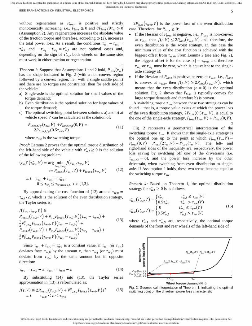
Theorem 1: Suppose that Assumptions 1 and 2 hold, 𝑃𝑙𝑜𝑠𝑠(𝜏𝑤) has the shape indicated in Fig. 2 (with a non-convex region

followed by a convex region, i.e., with a single saddle point)

and there are no torque rate constraints; then for each side of

the vehicle:

a) Single-axle is the optimal solution for small values of the

torque demand;

b) Even distribution is the optimal solution for large values of

the torque demand;

c) The optimal switching point between solutions a) and b) at

vehicle speed 𝑉 can be calculated as the solution of:

𝑃𝑙𝑜𝑠𝑠,𝑡 𝑔⁄ (𝜏𝑠𝑤 , 𝑉) +𝑃𝑙𝑜𝑠𝑠,𝑡/𝑔(0, 𝑉) =

2𝑃𝑙𝑜𝑠𝑠,𝑡 𝑔⁄ (0.5𝜏𝑠𝑤 , 𝑉) (11)

where 𝜏𝑠𝑤 is the switching torque.

Proof: Lemma 2 proves that the optimal torque distribution of

the left-hand side of the vehicle with 𝜏𝑤,𝑙∗ ≥ 0 is the solution

of the following problem:


∗ , 𝑉) = arg min𝜏𝑤1 ,𝜏𝑤3

𝐽(𝜏𝑤1 , 𝜏𝑤3 , 𝑉)

∶= 𝑃𝑙𝑜𝑠𝑠,𝑡(𝜏𝑤1 , 𝑉) + 𝑃𝑙𝑜𝑠𝑠,𝑡(𝜏𝑤3 , 𝑉)

𝑠. 𝑡. 𝜏𝑤1 + 𝜏𝑤3 = 𝜏𝑤,𝑙∗ ;

0 ≤ 𝜏𝑤𝑖 ≤ 𝜏𝑤,𝑚𝑎𝑥,𝑖,𝑡; 𝑖 ∈ {1,3}.

(12)

By approximating the cost function of (12) around 𝜏𝑤,0 =

𝜏𝑤,𝑙∗ /2, which is the solution of the even distribution strategy,

the Taylor series is:

𝐽(𝜏𝑤1 , 𝜏𝑤3 , 𝑉) ≅

𝑃𝑙𝑜𝑠𝑠,𝑡(𝜏𝑤,0, 𝑉) + ∇𝜏𝑤𝑃𝑙𝑜𝑠𝑠,𝑡(𝜏𝑤,0, 𝑉)(𝜏𝑤1 − 𝜏𝑤,0) +1

2∇𝜏𝑤𝜏𝑤2 𝑃𝑙𝑜𝑠𝑠,𝑡(𝜏𝑤,0, 𝑉)(𝜏𝑤1 − 𝜏𝑤,0)

2+

𝑃𝑙𝑜𝑠𝑠,𝑡(𝜏𝑤,0, 𝑉) + ∇𝜏𝑤𝑃𝑙𝑜𝑠𝑠,𝑡(𝜏𝑤,0, 𝑉)(𝜏𝑤3 − 𝜏𝑤,0) +1

2∇𝜏𝑤𝜏𝑤2 𝑃𝑙𝑜𝑠𝑠,𝑡(𝜏𝑤,0, 𝑉)(𝜏𝑤3 − 𝜏𝑤,0)

2

(13)

Since 𝜏𝑤1 + 𝜏𝑤3 = 𝜏𝑤,𝑙∗ is a constant value, if 𝜏𝑤1 (or 𝜏𝑤3)

deviates from 𝜏𝑤,0 by the amount 휀, then 𝜏𝑤3 (or 𝜏𝑤1) must

deviate from 𝜏𝑤,0 by the same amount but in opposite

direction:

𝜏𝑤1 = 𝜏𝑤,0 + 휀; 𝜏𝑤3 = 𝜏𝑤,0 − 휀 (14)

By substituting (14) into (13), the Taylor series

approximation in (13) is reformulated as:

𝐽(휀, 𝑉) ≅ 2𝑃𝑙𝑜𝑠𝑠,𝑡(𝜏𝑤,0, 𝑉) + ∇𝜏𝑤𝜏𝑤2 𝑃𝑙𝑜𝑠𝑠,𝑡(𝜏𝑤,0, 𝑉)휀

2

𝑠. 𝑡. −𝜏𝑤,0 ≤ 휀 ≤ 𝜏𝑤,0

(15)

2𝑃𝑙𝑜𝑠𝑠(𝜏𝑤,0, 𝑉) is the power loss of the even distribution

case. Therefore, for 𝑃𝑙𝑜𝑠𝑠 ≥ 0:

If the Hessian of 𝑃𝑙𝑜𝑠𝑠 is negative, i.e., 𝑃𝑙𝑜𝑠𝑠 is non-convex

at 𝜏𝑤,0, then 𝐽(휀, 𝑉) ≤ 2𝑃𝑙𝑜𝑠𝑠(𝜏𝑤,0, 𝑉) and, therefore, the

even distribution is the worst strategy. In this case the

minimum value of the cost function is achieved with the

biggest offset from 𝜏𝑤,0. From Lemma 2 (see also Fig. 2),

the biggest offset is for the case |휀| = 𝜏𝑤,0, and therefore

𝜏𝑤1 or 𝜏𝑤3 must be zero, which is equivalent to the single-

axle strategy a);

If the Hessian of 𝑃𝑙𝑜𝑠𝑠 is positive or zero at 𝜏𝑤,0, i.e., 𝑃𝑙𝑜𝑠𝑠

is convex at 𝜏𝑤,0, then 𝐽(휀, 𝑉) ≥ 2𝑃𝑙𝑜𝑠𝑠(𝜏𝑤,0, 𝑉), which

means that the even distribution (휀 = 0) is the optimal

solution. Fig. 2 shows that 𝑃𝑙𝑜𝑠𝑠 is typically convex for

large torque demands and therefore b) is proven.

A switching torque 𝜏𝑠𝑤 between these two strategies can be

found – that is, a torque value exists at which the power loss

of the even distribution strategy, 2𝑃𝑙𝑜𝑠𝑠(0.5𝜏𝑠𝑤 , 𝑉), is equal to

the one of the single-axle strategy, 𝑃𝑙𝑜𝑠𝑠(𝜏𝑠𝑤 , 𝑉) + 𝑃𝑙𝑜𝑠𝑠(0, 𝑉). □

Fig. 2 represents a geometrical interpretation of the

switching torque 𝜏𝑠𝑤. It shows that the single-axle strategy is

the optimal one up to the point at which 𝑃𝑙𝑜𝑠𝑠(𝜏𝑤 , 𝑉) −𝑃𝑙𝑜𝑠𝑠(0, 𝑉) = 𝑃𝑙𝑜𝑠𝑠(2𝜏𝑤 , 𝑉) − 𝑃𝑙𝑜𝑠𝑠(𝜏𝑤 , 𝑉). The left- and

right-hand sides of the inequality are, respectively, the power

loss saving by switching off one of the drivetrains (i.e.

𝜏𝑤,1/3 = 0), and the power loss increase by the other

drivetrain, when switching from even distribution to single-

axle. If Assumption 2 holds, these two terms become equal at

the switching torque 𝜏𝑠𝑤.

Remark 4: Based on Theorem 1, the optimal distribution

strategy for 𝜏𝑤,𝑙∗ ≥ 0 is as follows:

𝜏𝑤,1∗ (𝜏𝑤,𝑙

∗ , 𝑉) = {𝜏𝑤,𝑙∗ 𝜏𝑤,𝑙

∗ ≤ 𝜏𝑠𝑤(𝑉)

0.5𝜏𝑤,𝑙∗ 𝜏𝑤,𝑙

∗ > 𝜏𝑠𝑤(𝑉)

𝜏𝑤,3∗ (𝜏𝑤,𝑙

∗ , 𝑉) = {0 𝜏𝑤,𝑙

∗ ≤ 𝜏𝑠𝑤(𝑉)

0.5𝜏𝑤,𝑙∗ 𝜏𝑤,𝑙

∗ > 𝜏𝑠𝑤(𝑉)

(16)

where 𝜏𝑤,1∗ and 𝜏𝑤,3

∗ are, respectively, the optimal torque

demands of the front and rear wheels of the left-hand side of

Fig. 2. Geometrical interpretation of Theorem 1, indicating the optimal switching point on the drivetrain power loss characteristic




6

the vehicle. In the single-axle strategy the front motors are

selected (instead of the rear motors) for safety reasons; in fact,

in limit conditions it is preferable to have understeer rather

than oversteer.

The equivalent right-hand side torques are calculated with

the same approach. In the practical implementation of the

controller, a sigmoid function is used to approximate the

discontinuity of (16), in order to prevent drivability issues

deriving from the fast variation of the torque demands.

Remark 5: 𝜏𝑠𝑤 depends on the value of 𝑉. Since the problem

is parametric, the solution is parametric as well. In practice, 𝑉

can be estimated with a suitable Kalman filter using the four

wheel speeds and the longitudinal acceleration of the vehicle.

[24-25] describe methods for vehicle speed estimation.

Remark 6: If 𝑃𝑙𝑜𝑠𝑠(𝜏𝑤) is convex (i.e., without the saddle point

in Fig. 2), then the even distribution is the optimal solution for

any torque demand.

Remark 7: If (13) is not a good approximation of

𝐽(𝜏𝑤1 , 𝜏𝑤3 , 𝑉), the even order derivatives of 𝑃𝑙𝑜𝑠𝑠,𝑡(𝜏𝑤 , 𝑉) with

respect to 𝜏𝑤 must either be zero or have the same sign for a

given value of 𝜏𝑤. For example, this is the case if

𝑃𝑙𝑜𝑠𝑠,𝑡(𝜏𝑤, 𝑉) is a cubic polynomial. The experimental power

loss characteristics reported in Section IV are well interpolated

by a cubic polynomial.

Remark 8: The developed control allocation strategy is

overruled in two cases:

In the case of wheel torque saturation (see Section II.B),

the torque demand beyond the limit is transferred to the

other wheel on the same side until saturation is reached as

well;

For significant braking, an Electronic Braking Distribution

(EBD) strategy intervenes to maintain the correct relative

slip ratio among the tires of the front and rear axles.

IV. RESULTS

A. Experiments

Experimental system setup

Fig. 3 shows the experimental set-up for the validation of the

developed torque distribution strategy. The vehicle

demonstrator is an electric Range Rover Evoque with four

identical on-board switched reluctance motors, connected to

the wheels through single-speed transmissions, constant-

velocity joints and half-shafts. Table I reports the main vehicle

parameters.

A dSPACE AutoBox system is used for running all

controllers (Fig. 1), including the reference generator, the

high-level controller (as in [26]) and the CA algorithm. The

electrical power is provided by an external supply (visible in

the background of Fig. 3), which is connected in parallel with

the battery pack. Therefore, the high-voltage dc bus level is

maintained steady around 600 V.

Fig. 3. The Range Rover Evoque set-up on the rolling road facility at Flanders MAKE (Belgium)

The tests were conducted using a MAHA rolling road

facility (located at Flanders MAKE, Belgium) allowing speed

and torque control modes of the rollers. In the speed control

mode, the roller speeds are constantly kept at the specified set

value irrespective of variations in the actual wheel torques.

The torque demand at each wheel is assigned manually

through the dSPACE interface, and therefore the vehicle can

be tested for any assigned achievable torque demand and

speed. The rig includes the measurement of the longitudinal

force and speed of the rollers, and thus allows the evaluation

of the overall drivetrain efficiency, i.e., from the electrical

power at the inverters to the mechanical power at the rollers

during traction (opposite flow in the case of regeneration). In

the torque control mode, the roller bench applies a torque to

the rollers, which emulates tire rolling resistance, aerodynamic

drag and vehicle inertia. Therefore, the torque control mode is

used for driving cycle testing. The vehicle follows the

reference velocity profile of the specific driving schedule

through a velocity trajectory tracker (i.e., a model of the

human driver) implemented on the dSPACE system as the

combination of a feedforward and feedback controller,

providing a wheel torque demand output.

Drivetrain power loss measurement

The experimental drivetrain power loss characteristics of the

case study EV are reported in Fig. 4 for a number of vehicle

speeds. The power loss curves are plotted in terms of the

actual wheel torque. The first point of each curve corresponds

to the case of zero wheel torque demand, resulting in non-zero

power loss due to tire rolling resistance; conversely, the actual

wheel torque is zero when the torque supplied by drivetrain

compensates rolling resistance.

TABLE I. MAIN VEHICLE PARAMETERS

Symbol Name and dimension Value

ℓ Wheelbase (m) 2.665

𝜏𝑔𝑏 Gearbox ratio (-) 10.56

𝑅 Wheel radius (m) 0.364

𝑑 Half-track (m) 0.808

− No. of motors per axle (-) 2

𝑉𝑑𝑐 High-voltage dc bus level (V) 600

𝑇𝑛 Motor nominal torque (Nm) 80

𝑃𝑛 Motor nominal power (kW) 35

𝑃𝑝 Motor peak power (kW) 75




7

Fig. 4 shows that the drivetrain power loss characteristics

are positive and strictly monotonically increasing functions of

wheel torque, hence, confirming Assumption 2. The curves are

non-convex for low wheel torques and become convex for

large torque values. Therefore, Theorem 1 is applicable to the

design of an energy-efficient CA algorithm for the electric

Range Rover Evoque demonstrator. Fig. 5 reports the

measured efficiencies of each side of the EV demonstrator in

terms of the front-to-total torque ratio, for different values of

𝑉 and side torque demands. The relative slip among the

wheels does not change significantly for the different

combinations of speeds, torque demands and front-to-total

torque ratios. Due to the non-convexity of the power loss at

low torque demands, the efficiency is higher for torque ratios

of 0 or 1, i.e., for the single-axle strategy. In contrast, an even

distribution (corresponding to the torque ratio of 0.5) is the

optimal solution for high torque demands. As a result, the

optimal torque distribution on each side of the vehicle is

achieved by switching between the single-axle and even

distribution strategies depending on torque demand and

vehicle speed.

Switching torque calculation

Based on the measured power loss curves in Fig. 4, the

switching torque, 𝜏𝑠𝑤, is calculated using Theorem 1 and (11).

The power loss curve at each vehicle speed is piecewise

linearly interpolated to construct 𝑃𝑙𝑜𝑠𝑠(𝜏𝑤 , 𝑉). The method

assumes that the tire rolling resistance power losses are equal

at each vehicle corner, which is a reasonable approximation in

normal driving conditions with low values of the load transfers

(which directly affect tire power losses). The longitudinal slip

power losses are included in the rolling road measurement.

The method assumes that the slip ratios are similar to those

measured on the rolling road, which is also a reasonable

approximation in normal driving conditions. Knowing

𝑃𝑙𝑜𝑠𝑠(𝜏𝑤 , 𝑉), (11) is solved offline with an exhaustive search

method to calculate 𝜏𝑠𝑤. Fig. 6 shows the calculated 𝜏𝑠𝑤 on

each side of the vehicle for different 𝑉. The values were stored

as a look-up table in the controller running on the dSPACE

system. In terms of implementation on the vehicle, the

developed procedure is fast, i.e., it can easily be run in real-

time on hardware with low computational processing power.

Fig. 4. The power losses of a single drivetrain, measured on the rolling road facility

Fig. 5. Measured drivetrain efficiencies as a function of the front-to-total torque ratio, for different side torques at vehicle speeds of: (a) 40 km/h; (b) 65 km/h; (c) 90 km/h; and (d) 115 km/h

Fig. 6. Switching torque (τsw) for each side of the vehicle as a function

of V

Driving cycle tests

To assess the energy-efficiency benefits of the developed CA

strategy in straight line conditions, three different driving

cycles were performed with the vehicle demonstrator on the

rolling road. The driving cycles are the New European Driving

Cycle (NEDC), the Artemis Road driving cycle, and the Extra

Urban Driving Cycle (EUDC) with the hypothesis of a

constant 8% (uphill) slope of the road.

0 100 200 300 400 500 600 700 8000

10

20

30

40140 km/h

120 km/h

105 km/h

75 km/h

37.5 km/h

0 0.5 10

0.2

0.4

0.6

0.8

1

0 0.5 10

0.2

0.4

0.6

0.8

1

0 0.5 10

0.2

0.4

0.6

0.8

1

0 0.5 10

0.2

0.4

0.6

0.8

1

650 Nm

250 Nm

100 Nm

550 Nm

200 Nm

75 Nm

800 Nm

550 Nm

125 Nm

700 Nm

275 Nm

150 Nm

20 40 60 80 100 120 140250

300

350

400

450

500

550

600

650

TABLE II. ENERGY CONSUMPTION OF THE DEVELOPED CONTROL ALLOCATION STRATEGY OVER DIFFERENT DRIVING

CYCLES

Driving

Cycle

Energy consumptions (kWh) Improvements (%) of

CA with respect to

Single-

axle only

Even

distribution

With

CA

Single-

axle only

Even

distribution

NEDC 2.921 3.059 2.918 0.1% 4.6%

Artemis-

Road 4.487 4.634 4.442 1.0% 4.1%

EUDC 8%

slope 5.793 5.740 5.709 1.5% 0.5%




8

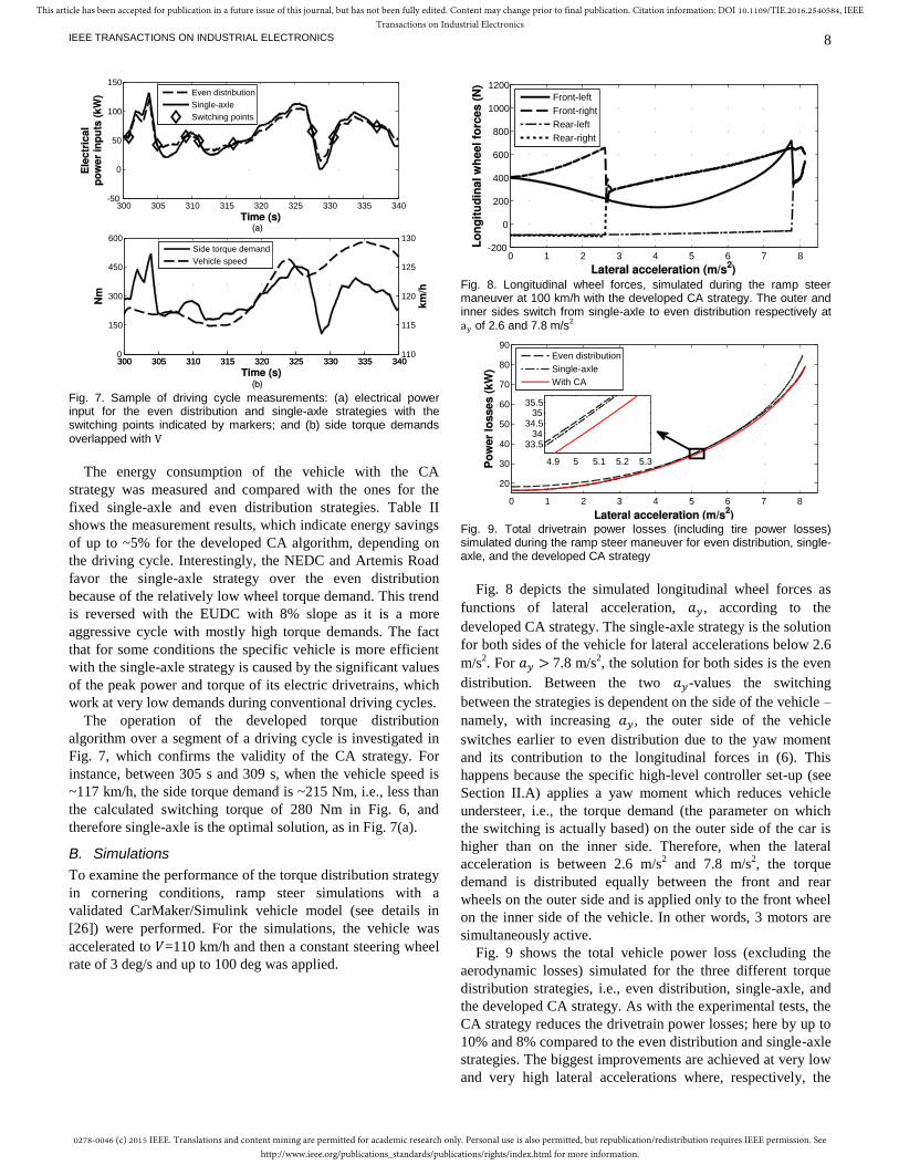
Fig. 7. Sample of driving cycle measurements: (a) electrical power input for the even distribution and single-axle strategies with the switching points indicated by markers; and (b) side torque demands

overlapped with V

The energy consumption of the vehicle with the CA

strategy was measured and compared with the ones for the

fixed single-axle and even distribution strategies. Table II

shows the measurement results, which indicate energy savings

of up to ~5% for the developed CA algorithm, depending on

the driving cycle. Interestingly, the NEDC and Artemis Road

favor the single-axle strategy over the even distribution

because of the relatively low wheel torque demand. This trend

is reversed with the EUDC with 8% slope as it is a more

aggressive cycle with mostly high torque demands. The fact

that for some conditions the specific vehicle is more efficient

with the single-axle strategy is caused by the significant values

of the peak power and torque of its electric drivetrains, which

work at very low demands during conventional driving cycles.

The operation of the developed torque distribution

algorithm over a segment of a driving cycle is investigated in

Fig. 7, which confirms the validity of the CA strategy. For

instance, between 305 s and 309 s, when the vehicle speed is

~117 km/h, the side torque demand is ~215 Nm, i.e., less than

the calculated switching torque of 280 Nm in Fig. 6, and

therefore single-axle is the optimal solution, as in Fig. 7(a).

B. Simulations

To examine the performance of the torque distribution strategy

in cornering conditions, ramp steer simulations with a

validated CarMaker/Simulink vehicle model (see details in

[26]) were performed. For the simulations, the vehicle was

accelerated to 𝑉=110 km/h and then a constant steering wheel

rate of 3 deg/s and up to 100 deg was applied.

Fig. 8. Longitudinal wheel forces, simulated during the ramp steer maneuver at 100 km/h with the developed CA strategy. The outer and inner sides switch from single-axle to even distribution respectively at ay of 2.6 and 7.8 m/s

2

Fig. 9. Total drivetrain power losses (including tire power losses) simulated during the ramp steer maneuver for even distribution, single-axle, and the developed CA strategy

Fig. 8 depicts the simulated longitudinal wheel forces as

functions of lateral acceleration, 𝑎𝑦, according to the

developed CA strategy. The single-axle strategy is the solution

for both sides of the vehicle for lateral accelerations below 2.6

m/s2. For 𝑎𝑦 > 7.8 m/s

2, the solution for both sides is the even

distribution. Between the two 𝑎𝑦-values the switching

between the strategies is dependent on the side of the vehicle –

namely, with increasing 𝑎𝑦, the outer side of the vehicle

switches earlier to even distribution due to the yaw moment

and its contribution to the longitudinal forces in (6). This

happens because the specific high-level controller set-up (see

Section II.A) applies a yaw moment which reduces vehicle

understeer, i.e., the torque demand (the parameter on which

the switching is actually based) on the outer side of the car is

higher than on the inner side. Therefore, when the lateral

acceleration is between 2.6 m/s2 and 7.8 m/s

2, the torque

demand is distributed equally between the front and rear

wheels on the outer side and is applied only to the front wheel

on the inner side of the vehicle. In other words, 3 motors are

simultaneously active.

Fig. 9 shows the total vehicle power loss (excluding the

aerodynamic losses) simulated for the three different torque

distribution strategies, i.e., even distribution, single-axle, and

the developed CA strategy. As with the experimental tests, the

CA strategy reduces the drivetrain power losses; here by up to

10% and 8% compared to the even distribution and single-axle

strategies. The biggest improvements are achieved at very low

and very high lateral accelerations where, respectively, the

300 305 310 315 320 325 330 335 340-50

0

50

100

150

300 305 310 315 320 325 330 335 3400

150

300

450

600

300 305 310 315 320 325 330 335 340110

115

120

125

130

Side torque demand

Vehicle speed

Even distribution

Single-axle

Switching points

0 1 2 3 4 5 6 7 8-200

0

200

400

600

800

1000

1200

Front-left

Front-right

Rear-left

Rear-right

0 1 2 3 4 5 6 7 8

20

30

40

50

60

70

80

90Even distribution

Single-axle

With CA

4.9 5 5.1 5.2 5.3

33.534

34.535

35.5




9

single-axle strategy and the even distribution strategy are the

optimal solutions (see also Fig. 6). For lateral accelerations

between 2.6 and 7.8 m/s2, when the optimal solution for the

outer and inner vehicle sides are different (Fig. 8), the

developed CA strategy reduces the power loss by ~2.4% (Fig.

9).

V. CONCLUSION

The presented research work allows the following

conclusions, essential for the design of a fast, energy-efficient

and easily implementable torque allocation algorithm for four-

wheel-drive electric vehicles with equal drivetrains on the

front and rear axles:

For relatively small values of steering wheel angle, the

control allocation problem of a four-wheel-drive electric

vehicle with multiple motors can be independently solved

for the left- and right-hand sides of the vehicle;

If the power loss characteristics of the electric drivetrains

are strictly monotonically increasing functions of the

torque demand, the minimum consumption is achieved by

using a single motor on each side of the vehicle up to a

torque demand threshold, and an even torque distribution

among the front and rear motors above such threshold;

An analytical formula is proposed for the computation of

the torque demand threshold, which is a function of vehicle

speed, based on the drivetrain power loss characteristic;

The developed strategy is easily implementable as a small-

sized look-up table in the main control unit of the vehicle,

allowing real-time operation with minimum demand on the

processing hardware;

The experimental analysis of the case study drivetrain

efficiency characteristics as functions of the front-to-total

wheel torque distribution confirms the validity of the

proposed control allocation algorithm at different vehicle

velocities and torque demands, i.e., at low torques single-

axle is the optimal solution and at high torques even

distribution is the optimal solution;

The experimental results for a four-wheel-drive electric

vehicle demonstrator along driving cycles show energy

consumption reductions between 0.5% and 5%, with

respect to the same vehicle with single-axle or even torque

distributions;

The simulation results of ramp steer maneuvers indicate

significant energy consumption reductions for the whole

range of lateral accelerations.

The approximation related to the assumptions of tire slip

ratios similar to those in the rolling road experiments and

negligible rolling resistance variation with vertical load will be

addressed in future work.

REFERENCES

[1] Y. Wang, B.M. Nguyen, H. Fujimoto, and Y. Hori, "Multirate estimation

and control of body sideslip angle for electric vehicles based on onboard

vision system," IEEE Trans. Ind. Electron., vol. 61, no. 2, pp. 1133-1143,

2014. [2] K. Nam, S. Oh, and H. Fujimoto, "Estimation of sideslip and roll angles of

electric vehicles using lateral tire force sensors through RLS and Kalman

filter approaches," IEEE Trans. Ind. Electron., vol. 60, no. 3, pp. 988-1000, 2013.

[3] A. Pennycott, L. De Novellis, P. Gruber, A. Sorniotti, "Sources of Energy

Loss during Torque-Vectoring for Fully Electric Vehicles", Int. J. Veh. Des., vol. 67, no. 2, pp. 157-177, 2014.

[4] Y. Suzuki, Y. Kano, and M. Abe, "A study on tyre force distribution

controls for full drive-by-wire electric vehicle," Veh. Syst. Dyn., vol. 52, supp. 1, pp. 235-250, 2014.

[5] R. Wang, Y. Chen, D. Feng, X. Huang, and J. Wang, "Development and

performance characterization of an electric ground vehicle with independently actuated in-wheel motors," J. Power Sources, vol. 196, pp.

3962-3971, 2011.

[6] Y. Chen and J. Wang, "Adaptive Energy-Efficient Control Allocation for Planar Motion Control of Over-Actuated Electric Ground Vehicles,"

IEEE Trans. Contr. Syst. Technol., vol. 22, no. 4, pp. 1362-1373, 2014.

[7] A. Pennycott, L. De Novellis, A. Sabbatini, P. Gruber, and A. Sorniotti, "Reducing the motor power losses of a four-wheel drive, fully electric

vehicle via wheel torque allocation," Proc. Inst. Mech. Eng., Part D: J.

Autom. Eng., vol. 228, no. 7, pp. 830-839, 2014. [8] X. Yuan and J. Wang, "Torque Distribution Strategy for a Front- and

Rear-Wheel-Driven Electric Vehicle," IEEE Trans. Vehicul. Technol.,

vol. 61, no. 8, pp. 3365-3374, 2012. [9] L. De Novellis, A. Sorniotti, and P. Gruber, "Wheel Torque Distribution

Criteria for Electric Vehicles With Torque-Vectoring Differentials," IEEE

Trans. Vehicul. Technol., vol. 63, no. 4, pp. 1593-1602, 2014. [10] H. Fujimoto and S. Harada, "Model-Based Range Extension Control

System for Electric Vehicles With Front and Rear Driving-Braking Force

Distributions," IEEE Trans. Ind. Electron., vol. 62, no. 5, pp. 3245-3254, 2015.

[11] Y. Chen and J. Wang, "Fast and Global Optimal Energy-Efficient Control Allocation With Applications to Over-Actuated Electric Ground

Vehicles," IEEE Trans. Contr. Syst. Technol., vol. 20, no. 5, pp. 1202-

1211, 2012. [12] Y. Chen and J. Wang, "Design and Experimental Evaluations on Energy

Efficient Control Allocation Methods for Overactuated Electric Vehicles:

Longitudinal Motion Case," IEEE/ASME Trans. Mechatron., vol. 19, no. 2, pp. 538-548, 2014.

[13] Y. Chen and J. Wang, "Energy-efficient control allocation with

applications on planar motion control of electric ground vehicles," Americ. Contr. Conf., pp. 2719-2724, 2011.

[14] S. Fallah, A. Khajepour, B. Fidan, C. Shih-Ken, and B. Litkouhi,

"Vehicle Optimal Torque Vectoring Using State-Derivative Feedback and Linear Matrix Inequality," IEEE Trans. Vehicul. Technol., vol. 62, no. 4,

pp. 1540-1552, 2013.

[15] B. Li, A. Goodarzi, A. Khajepour, S.K. Chen, and B. Litkouhi, "An optimal torque distribution control strategy for four-independent wheel

drive electric vehicles," Veh. Syst. Dyn., vol. 53, no. 8, pp. 1-18, 2015.

[16] P. Tøndel and T. A. Johansen, "Control allocation for yaw stabilization in automotive vehicles using multiparametric nonlinear programming,"

Americ. Contr. Conf., pp. 453-458, 2005.

[17] T. A. Johansen, T. P. Fuglseth, P. Tøndel, and T. I. Fossen, "Optimal constrained control allocation in marine surface vessels with rudders,"

Contr. Eng. Practice, vol. 16, no. 4, pp. 457-464, 2008.

[18] J. Tjønnås and T. A. Johansen, "Adaptive control allocation," Automatica, vol. 44, no. 11, pp. 2754-2765, 2008.

[19] J. Tjonnas and T. A. Johansen, "Stabilization of Automotive Vehicles

Using Active Steering and Adaptive Brake Control Allocation," IEEE Trans. Contr. Syst. Technol., vol. 18, no. 3, pp. 545-558, 2010.

[20] T. A. Johansen and T. I. Fossen, "Control allocation—A survey,"

Automatica, vol. 49, no. 5, pp. 1087-1103, 2013. [21] O. Härkegård and S. T. Glad, "Resolving actuator redundancy—optimal

control vs. control allocation," Automatica, vol. 41, no. 1, pp. 137-144,

2005. [22] L. F. Domínguez, D. A. Narciso, and E. N. Pistikopoulos, "Recent

advances in multiparametric nonlinear programming," Comput. & Chem.

Eng., vol. 34, no. 5, pp. 707-716, 2010. [23] A. Grancharova and T. A. Johansen, "Multi-parametric Programming," in

Explicit Nonlinear Model Predictive Control - Theory and Applications.

vol. 429, Springer, pp. 1-37, 2012.

[24] U. Kiencke and L. Nielsen, "Automotive control systems: for engine,

driveline, and vehicle," Springer, 2005.

[25] M. Tanelli, S. M. Savaresi, and C. Cantoni, "Longitudinal vehicle speed estimation for traction and braking control systems," IEEE Int. Conf. on

Contr. Applic., pp. 2790-2795, 2006.

[26] L. De Novellis, A. Sorniotti, P. Gruber, J. Orus, J.-M. Rodriguez Fortun, J. Theunissen, and J. De Smet, "Direct yaw moment control actuated




10

through electric drivetrains and friction brakes: Theoretical design and

experimental assessment," Mechatronics, vol. 26, pp. 1-15, 2015.

Arash M. Dizqah (M'12) received the B.Sc. and M.Sc. degrees in electrical engineering from Sharif University and K.N. Toosi University, Tehran, Iran, in 1998 and 2001, respectively, and the Ph.D. degree in control engineering from Northumbria University, UK, in 2014. He was Research Fellow with the University of Surrey, UK. He is a Lecturer in intelligent transport systems with Coventry University, UK. His research interests are decentralized control

and optimization, and nonlinear model-predictive controllers for connected vehicles, electric and hybrid vehicles and renewable energy systems.

Basilio Lenzo (M’13) received the M.Sc. degree in mechanical engineering from the University of Pisa and Scuola Superiore Sant'Anna, Pisa, Italy, in 2010, and the Ph.D. degree in robotics from Scuola Superiore Sant'Anna, Pisa, Italy, in 2013. In 2010 he was R&D Intern with Ferrari F1. In 2013 he was Visiting Researcher at the University of Delaware, USA, and Columbia University, USA. In late 2013 he was appointed Research

Fellow at Scuola Superiore Sant'Anna, where he worked on kinematics and dynamics of robotic mechanisms. Since 2015, he has been a Research Fellow with the Centre for Automotive Engineering, University of Surrey, Guildford, UK. His current research interests include vehicle dynamics, simulation, control and robotics.

Aldo Sorniotti (M’12) received the M.Sc. degree in mechanical engineering and the Ph.D. degree in applied mechanics from the Politecnico di Torino, Turin, Italy, in 2001 and 2005, respectively. He is a Reader in advanced vehicle engineering with the University of Surrey, Guildford, UK, where he is the coordinator of the Centre for Automotive Engineering. His research interests include vehicle dynamics control, integration of chassis

control systems, and transmission systems for electric and hybrid electric vehicles.

Patrick Gruber received the M.Sc. degree in motorsport engineering and management from Cranfield University, Cranfield, UK, in 2005 and the Ph.D. degree in mechanical engineering from the University of Surrey, Guildford, UK, in 2009. He is Senior Lecturer in advanced vehicle systems engineering with the University of Surrey. His current research interests include tire dynamics and development of novel tire models.

Saber Fallah received the B.Sc. degree from Isfahan University of Technology, Isfahan, Iran; the M.Sc. degree from Shiraz University, Shiraz, Iran; and the Ph.D. degree from Concordia University, Montreal, Canada, all in the field of mechanical engineering. He is a Lecturer with the University of Surrey, Guildford, UK. His research interests include vehicle dynamics and control, electric and hybrid electric vehicles, intelligent vehicles, and vehicle system design and integration.

Jasper De Smet received the M.Sc degree in electrical engineering from KU Leuven (Campus De Nayer), Sint-Katelijne-Waver, Belgium, in 2008. After graduation he had a one-year internship at Eurocopter, France. Since 2009, he has been a Researcher with Flanders MAKE, Lommel, Belgium. His research interests include integration and control of electro-mechanical systems in vehicles and machines.

A Fast and Parametric Torque Distribution Strategy for ... · PDF fileof energy dissipations...

Documents

Transcript of A Fast and Parametric Torque Distribution Strategy for ... · PDF fileof energy dissipations...