A Dynamical Systems Modelfor Language Change

Partha Niyogi and Robert C. Berwick

Artificial Intelligence LaboratoryCenter for Biological and Computational LearningMassachusetts Institute of TechnologyCambridge, MA 02139email: niyogi@research.bell-labs.com, berwick@ai.mit.edu

Abstract

This paper formalizes linguists’ intuitions about language change,proposing a dynamical systems model for language change derivedfrom a model for language acquisition. Linguists must explain not onlyhow languages are learned but also how and why they have evolvedalong certain trajectories and not others. While the language learn-ing problem has focused on the behavior of individuals and how theyacquire a particular grammar from a class of grammars G, here weconsider a population of such learners and investigate the emergent,global population characteristics of linguistic communities over severalgenerations. We argue that language change follows logically from spe-cific assumptions about grammatical theories and learning paradigms.Roughly, as the end product of two types of learning misconvergenceover several generations, individual language learner behavior leads toemergent, population language community characteristics.

In particular, we show that any triple {G,A,P} of grammaticaltheory, learning algorithm, and initial sentence distributions can betransformed into a dynamical system whose evolution depicts a pop-ulation’s evolving linguistic composition. We explicitly show how thistransformation can be carried out for memoryless learning algorithmsand parameterized grammatical theories. As the simplest case, we for-malize the example of two grammars (languages) differing by exactlyone binary parameter, and show that even this situation leads directlyto a quadratic (nonlinear) dynamical system, including regions withchaotic behavior. We next apply the computational model to some

some actual data, namely the observed historical loss of “Verb Sec-ond” from Old French to modern French. Thus, the formal modelallows one to pose new questions about language phenomena that oneotherwise could not ask, such as: (1) whether languages/grammarscorrectly follow observed historical trajectories—an evolutionary cri-teria for the adequacy of grammatical theories; (2) what are the logi-cally possible dynamical change envelopes given a posited grammaticaltheory—rates and shapes of linguistic change, including the possibili-ties for the past and the future; (3) what can be the effect of quantifiedvariation in initial conditions (e.g., population differences resultingfrom socio-political facts); (4) intrinsically interesting mathematicalquestions regarding linguistic dynamical systems.

1

1 Introduction: The Paradox of Language Change

Much research on language has focused on how children acquire the grammarof their parents from “impoverished” data presented to them during child-hood. The logical problem of language acquisition, cast formally, requires thelearner to converge (attain) its correct target grammar (i.e., the language ofits caretakers, that belongs to a class of possible natural language gram-mars). However this learnability problem, if solved perfectly, would lead toa paradox: If generation after generation children successfully attained thegrammar of their parents, then languages would never change with time. Yetlanguages do change.

Language scientists have long been occupied with describing phonologi-cal, syntactic, and semantic change, often appealing to an analogy betweenlanguage change and evolution, but rarely going beyond this. For instance,Lightfoot (1991, chapter 7, pp. 163–65ff.) talks about language change inthis way: “Some general properties of language change are shared by otherdynamic systems in the natural world . . . In population biology and linguis-tic change there is constant flux. . . . If one views a language as a totality, ashistorians often do, one sees a dynamic system”. Indeed, entire books havebeen devoted to the description of language change using the terminology ofpopulation biology: genetic drift, clines, and so forth1 Other scientists haveexplicitly made an appeal to dynamical systems in this context; see espe-cially Hawkins and Gell-Mann, 1989. Yet to the best of our knowledge, theseintuitions have not been formalized. That is the goal of this paper.

In particular, we show formally that a model of language change emergesas a logical consequence of language acquisition, an argument made infor-mally by Lightfoot (1991). We shall see that Lightfoot’s intuition that lan-guages could behave just as though they were dynamical systems is essen-tially correct, as is his proposal for turning language acquisition models intolanguage change models. We can provide concrete examples of both “grad-ual” and “sudden” syntactic changes, occurring over time periods of manygenerations to just a single generation.2

Many interesting points emerge from the formalization, some empirical,

1For a recent example, see Nichols (1992), Linguistic Diversity in Space and Time.2Lightfoot 1991 refers to these sudden changes acting over a single generation as “catas-

trophic” but in fact this term usually has a different sense in the dynamical systemsliterature.

2

some programmatic:

1. Learnability is a well-known criterion for the adequacy of grammaticaltheories. Our model provides an evolutionary criterion: By comparingthe trajectories of dynamical linguistic systems to historically observedtrajectories, one can determine the adequacy of linguistic theories orlearning algorithms.

2. We derive explicit dynamical systems corresponding to parametrizedlinguistic theories (e.g., the Head First/Final parameter in head-drivenphrase structure grammars or government-binding grammars) and mem-oryless language learning algorithms (e.g., gradient ascent in parameterspace).

3. In the simplest possible case of a 2-language (grammar) system differ-ing by exactly 1 binary parameter, the system reduces to a quadraticmap with the usual chaotic properties (dependent on initial conditions).That such complexity can arise even in the simplest case suggests thatformally modeling language change may be quite mathematically rich.

4. We illustrate the use of dynamical systems as a research tool by con-sidering the loss of Verb Second position in Old French as compared toModern French. We demonstrate by computer modeling that one gram-matical parameterization advanced in the linguistics literature does notseem to permit this historical change, while another does.

5. We can more accurately model the time course of language change. Inparticular, in contrast to Kroch (1990) and others, who mimic popu-lation biology models by imposing an S-shaped logistic change by as-sumption, we explain the time course of language change, and show thatit need not be S-shaped. Rather, language-change envelopes are deriv-able from more fundamental properties of dynamical systems; some-times they are S-shaped, but they can also be nonmonotonic.

6. We examine by simulation and traditional phase-space plots the formand stability of possible “diachronic envelopes” given varying alterna-tive language distributions, language acquisition algorithms, parame-terizations, input noise, and sentence distributions. The results bear

3

on models of language “mixing”; so-called “wave” models for languagechange; and other proposals in the diachronic literature.

7. As topics for future research, the dynamical system model providesa novel possible source for explaining several linguistic changes includ-ing: (a) the evolution of modern Greek metrical stress assignment fromproto-Indo-European; and (b) Bickerton’s (1990) “creole hypothesis,”concerning the striking fact that all creoles, irrespective of linguisticorigin, have exactly the same grammar. In the latter case, the “uni-versality” of creoles could be due a parameterization corresponding toa common condensation point of a dynamical system, a possibility notconsidered by Bickerton.

2 An Acquisition-Based Model of Language

Change

How does the combination of a grammatical theory and learning algorithmlead to a model of language change? We first note that just as with languageacquisition, there is a seeming paradox in language change: it is generally as-sumed that children acquire their caretaker (target) grammars without error.However, if this were always true, at first glance grammatical changes withina population could seemingly never occur, since generation after generationchildren would successfully acquire the grammar of their parents.

Of course, Lightfoot and others have pointed out the obvious solutionto this paradox: the possibility of slight misconvergence to target grammarscould, over several generations, drive language change, much as speciationoccurs in the population biology sense:

As somebody adopts a new parameter setting, say a new verb-object order, the output of that person’s grammar often differsfrom that of other people’s. This in turn affects the linguisticenvironment, which may then be more likely to trigger the newparameter setting in younger people. Thus a chain reaction maybe created. (Lightfoot, 1991, p. 162)

We pursue this point in detail below. Similarly, just as in the biologicalcase, some of the most commonly observed changes in languages seem to

4

occur as the result of the effects of surrounding populations, whose featuresinfiltrate the original language.

We begin our treatment by arguing that the problem of language acquisi-tion at the individual level leads logically to the problem of language changeat the group or population level. Consider a population speaking a particularlanguage3. This is the target language—children are exposed to primary lin-guistic data (PLD) from this source, typically in the form of sentences utteredby caretakers (adults). The logical problem of language acquisition is howchildren acquire this target language from their primary linguistic data—tocome up with an adequate learning theory. We take a learning theory tobe simply a mapping from primary linguistic data to the class of grammars,usually effective, and so an algorithm. For example, in a typical inductiveinference model, given a stream of sentences, an acquisition algorithm wouldsimply update its grammatical hypothesis with each new sentence accordingto some preprogrammed procedure. An important criterion for learnability(Gold, 1967) is to require that the algorithm converge to the target as thedata goes to infinity (identification in the limit).

Now suppose that we fix an adequate grammatical theory and an ade-quate acquisition algorithm. There are then essentially two means by whichthe linguistic composition of the population could change over time. First, ifthe primary linguistic data presented to the child is altered (due to any num-ber of causes, perhaps to presence of foreign speakers, contact with anotherpopulation, disfluencies, and the like), the sentences presented to the learner(child) are no longer consistent with a single target grammar. In the faceof this input, the learning algorithm might no longer converge to the targetgrammar. Indeed, it might converge to some other grammar (g2); or it mightconverge to g2 with some probability, g3 with some other probability, and soforth. In either case, children attempting to solve the acquisition problemusing the same learning algorithm could internalize grammars different fromthe parental (target) grammar. In this way, in one generation the linguisticcomposition of the population can change.4

3In our analysis this implies that all the adult members of this population have inter-nalized the same grammar (corresponding to the language they speak).

4Sociological factors affecting language change affect language acquisition in exactlythe same way, yet are abstracted away from the formalization of the logical problem oflanguage acquisition. In this same sense, we similarly abstract away such causes here,though they can be brought into the picture as variation in probability distributions and

5

Second, even if the PLD comes from a single target grammar, the actualdata presented to the learner is truncated, or finite. After a finite samplesequence, children may, with non-zero probability, hypothesize a grammardifferent from that of their parents. This can again lead to a differing lin-guistic composition in succeeding generations.

In short, the diachronic model is this: Individual children attempt to at-tain their caretaker target grammar. After a finite number of examples, someare successful, but others may misconverge. The next generation will there-fore no longer be linguistically homogeneous. The third generation of chil-dren will hear sentences produced by the second—a different distribution—and they, in turn, will attain a different set of grammars. Over successivegenerations, the linguistic composition evolves as a dynamical system.

On this view, language change is a logical consequence of specific assump-tions about:

1. the grammar hypothesis space—a particular parametrization, in a para-metric theory;

2. the language acquistion device—the learning algorithm the child usesto develop hypotheses on the basis of data;

3. the primary linguistic data—the sentences presented to the children ofany one generation.

If we specify (1) through (3) for a particular generation, we should, inprinciple, be able to compute the linguistic composition for the next gener-ation. In this manner, we can compute the evolving linguistic compositionof the population from generation to generation; we arrive at a dynamicalsystem. We now proceed to make this calculation precise. We first reviewa standard language acquisition framework, and then show how to derive adynamical system from it.

2.1 The Language Acquisition Framework

To formalize the model, we must first state our assumptions about grammat-ical theories, learning algorithms, and sentence distributions.

learning algorithms; we leave this open here as a topic for additional research.

6

1. Denote by G, a family of possible (target) grammars. Each grammarg ∈ G defines a language L(g) ⊆ Σ∗ over some alphabet Σ in the usual way.

2. Denote by P a distribution on Σ∗ according to which sentences aredrawn and presented to the learner. Note that if there is a well definedtarget, gt, and only positive examples from this target are presented to thelearner, then P will have all its measure on L(gt), and zero measure onsentences outside Suppose n examples are drawn in this fashion, one can thenlet Dn = (Σ∗)n be the set of all n-example data sets the learner might bepresented with. Thus, if the adult population is linguistically homogeneous(with grammar g1) then P = P1. If the adult population speaks 50 percentL(g1) and 50 percent L(g2) then P = 1

2P1 + 1

2P2.

3. Denote by A the acquisition algorithm that children use to hypothesizea grammar on the basis of input data. A can be regarded as a mappingfrom Dn to G. Acting on a particular presentation sequence dn ∈ Dn, thelearner posits a hypothesis A(dn) = hn ∈ G. Allowing for the possibility ofrandomization, the learner could, in general, posit hi ∈ G with probabilitypi for such a presentation sequence dn. The standard (stochastic version)learnability criterion (Gold, 1967) can then be stated as follows:

For every target grammar, gt ∈ G, with positive-only examples presentedaccording to P as above, the learner must converge to the target with prob-ability 1, i.e.,

Prob[A(dn) = gt] −→n→∞ 1

One particular way of formulating the learning algorithm is as a local gra-dient ascent search through a space of target languages (grammars) definedby a 1 dimensional n-length Boolean array of parameters, with each distinctarray fixing a particular grammar (language). With n parameters, there are2n possible grammars (languages). For example, English and Japanese differin that English is a so-called “Verb first” language, while Japanese is “Verbfinal.” Given this framework, we can state the so-called Triggering LearningAlgorithm of Gibson and Wexler (1994) as follows:

• [Initialize] Step 1. Start at some random point in the (finite) space ofpossible parameter settings, specifying a single hypothesized grammarwith its resulting extension as a language;

• [Process input sentence] Step 2. Receive a positive example sentencesi at time ti (examples drawn from the language of a single target

7

grammar, L(Gt)), from a uniform distribution on unembedded (nonre-cursive) sentences of the target language.

• [Learnability on error detection] Step 3. If the current grammar parses(generates) si, then go to Step 2; otherwise, continue.

• [Single-step hill climbing] Step 4. Select a single parameter uniformlyat random, to flip from its current setting, and change it (0 mappedto 1, 1 to 0) iff that change allows the current sentence to be analyzed ;otherwise, leave the current parameter settings unchanged.

• [Iterate] Step 5. Go to Step 2.

Of course, this algorithm carries out “identification in the limit” in thestandard terminology of learning theory (Gold, 1967); it does not halt in theconventional sense.

It turns out that if the learning algorithm A is memoryless (in the sensethat previous examplesentences are not stored), and G can be described bya finite number of parameters, then we can describe the learning system A,Gt, G as a Markov chain M with as many states as there are grammars in G.More specifically the states in M are in 1-1 correspondence with grammarsg ∈ G and the target grammar Gt corresponds to a particular target statest of M . The transition probabilities between states in M can be computedstraightforwardly based on set difference calculations between the languagescorresponding to the Markov chain states. We omit the details of this demon-stration here; for a simple, explicit calculation in the case of one parameter,see section 3. For a more detailed analysis of learnability issues for memory-less algorithms in finite parameter spaces, consult Niyogi (1995), chapter 4,appendix B or Niyogi and Berwick (1995).

2.2 From Language Learning to Popuation Dynamics

The framework for language learning has learners attempting to infer gram-mars on the basis of linguistic data. At any point in time, n, (i.e., afterhearing n examples) the learner has a current hypothesis, h, with probabilitypn(h). What happens when there is a population of learners? Since an ar-bitrary learner has a probability pn(h) of developing hypothesis h (for every

8

h ∈ G), it follows that a fraction pn(h) of the population of learners inter-nalize the grammar h after n examples. We therefore have a current state ofthe population after n examples. This state of the population might well bedifferent from the state of the parent population. Assume for now that aftern examples, maturation occurs, i.e., after n examples the learner retains thegrammatical hypothesis for the rest of its life. Then one would arrive at thestate of the mature population for the next generation.5 This new generationnow produces sentences for the following generation of learners according tothe distribution of grammars in its population. Then, the process repeats it-self and the linguistic composition of the population evolves from generationto generation.

We can now define a discrete time dynamical system by providing its twonecessary components:A State Space: a set of system states, S. Here the state space is thespace of possible linguistic compositions of the population. Each state isdescribed by a distribution Ppop on G describing the language spoken by thepopulation.6 At any given point in time, t, the system is in exactly one states ∈ S;An Update Rule: how the system states change from one time step to thenext. Typically, this involves specifying a function, f, that maps st ∈ S tost+1

7

For example, a typical linear dynamical system might consist of statevariables x (where x is a k-dimensional state vector) and a system of dif-ferential equations x′ = Ax (A is a matrix operator) which characterize theevolution of the states with time. RC circuits are a simple example of lineardynamical systems. The state (current) evolves as the capcitor dischargesthrough the resistor. Population growth models (for example, using logistic

5Maturation seems to be a reasonable hypothesis in this context. After all, it seemseven more unreasonable to imagine that learners are forever wandering around in hypoth-esis space. There is evidence from developmental psychology to suggest that this is thecase, and that after a certain point children mature and retain their current grammaticalhypotheses forever.

6As usual, one needs to be able to define a σ-algebra on the space of grammars, andso on. This is unproblematic for the cases considered here because the set of grammars isfinite.

7In general, this mapping could be fairly complicated. For example, it could dependon previous states, future states, and so forth; for reasons of space we do not consider allpossibilities here. For reference, see Strogatz, 1993.

9

equations) provide other examples.As a linguistic example, consider the three parameter syntactic space

described in Gibson and Wexler (1994). This system defines eight possible“natural” grammars; G has eight elements. We can picture a distribution onthis space as shown in fig. 1. In this particular case, the state space is

S = {P ∈ R8|8

∑

i=1

Pi = 1}

FIGURE 1 HERE

Here we interpret the state as the linguistic composition of the population.8

For example, a distribution that puts all its weight on grammar g1 and 0 ev-erywhere else indicates a homogeneous population that speaks a languagecorresponding to grammar g1. Similarly, a distribution that puts a probabil-ity mass of 1/2 on g1 and 1/2 on g2 denotes a population (nonhomogeneous)with half its speakers speaking a language corresponding to g1 and half speak-ing a language corresponding to g2.

To see in detail how the update rule may be computed, consider theacquisition algorithm, A. For example, given the state at time t, (Ppop,t),the distribution of speakers in the parental population, one can obtain thedistribution with which sentences from Σ∗ will be presented to the learner.To do this, imagine that the ith linguistic group in the population, speakinglanguage Li, produces sentences with distribution Pi. Then for any ω ∈ Σ∗,

the probability with which ω is presented to the learner is given by

P (ω) =∑

i

Pi(ω)Ppop,t(i)

This fixes the distribution with which sentences are presented to thelearner. The logical problem of language acquisition also assumes some suc-cess criterion for attaining the mature target grammar. For our purposes, wetake this as being one of two broad possibilities: either (1) the usual Goldscenario of identification in the limit, what we shall call the limiting sample

8Note that we do not allow for the possibility of a single learner having more than onehypothesis at a time; an extension to this case, in which individuals would more closelyresemble the “ensembles” of particles in a thermodynamic system is left for future research.

10

case; or (2) identification in a fixed, finite time, what we shall call the finitesample case.9

Consider case (2) first. Here, one draws n example sentences according todistribution P , and the acquisition algorithm develops hypotheses (A(dn) ∈G). One can, in principle, compute the probability with which the learnerwill posit hypothesis hi after n examples:

Finite Sample: Prob[A(dn) = hi] = pn(hi) (1)

The finite sample situation is always well defined—the probability pn alwaysexists.10.

Now turn to case (1), the limiting case. Here learnability requires pn(gt)to go to 1, for the unique target grammar, gt, if such a grammar exists.However, in general there need not be a unique target grammar since thelinguistic population can be nonhomogeneous. Even so, the following limitingbehavior might still exist:

Limiting Sample: limn→∞

Prob[A(dn) = hi] = p(hi) (2)

Turning from the individual child to the population, since the individ-ual child internalizes grammar hi ∈ G with probability pn(hi) in the “finitesample” case or with probability p(hi) “in the limit”, in a population ofsuch individuals one would therefore expect a proportion pn(hi) or p(hi) re-spectively to have internalized grammar hi. In other words, the linguisticcomposition of the next generation is given by Ppop,t+1(hi) = pn(hi) for thefinite sample case and by Ppop,t+1(hi) = p(hi) in the limiting sample case . Inthis fashion,

Ppop,t −→A Ppop,t+1

9Of course, a variety of other success criteria, e.g., convergence within some epsilon,or polynomial in the size of the target grammar, are possible; each leads to potentiallydifferent language change model. We do not pursue these alternatives here.

10This is easy to see for deterministic algorithms, Adet. Such an algorithm would havea precise behavior for every data set of n examples drawn. In our case, the examplesare drawn in i.i.d. fashion according to a distribution P on Σ∗. It is clear that pn(hi) =P [{dn|Adet(dn) = hi}]. For randomized algorithms, the case is trickier, though tedious,but the probability still exists because all the finite choice paths over all sequences oflength n is enumerable. Previous work (Niyogi and Berwick, 1993,1994a,1994b) showshow to compute pn for randomized memoryless algorithms.

11

Remarks.

1. For a Gold-learnable family of languages and a limiting sample as-sumption, homogeneous populations are always stable. This is simplybecause each child and therefore the entire population always eventu-ally converges to a single target grammar, generation after generation.

2. . However, the finite sample case is different from the limiting samplecase. Suppose we have solved the maturation problem, that is, weknow roughly the time, or number of examples N the learner takesto develop its mature (adult) hypothesis. In that case pN(h) is theprobability that a child internalizes the grammar h, and pN(h) is thepercentage of speakers of Lh in the next generation. Note that underthis finite sample analysis, even for a homogeneous population withall adults speaking a particular language (corresponding to grammar,g, say), pN(g) will not be 1—that is, there will be a small percentageof learners who have misconverged. This percentage could blow upover several generations, and we therefore have potentially unstablelanguages.

3. The formulation is very general. Any {A,G,P〉} triple yields a dynam-ical system.11. In short:

(G,A, {Pi}) −→ D( dynamical system)

4. The formulation also does not assume any particular linguistic theory,learning algorithm, or distribution with which sentences are drawn. Ofcourse, we have implicitly assumed a learning model, i.e., positive ex-amples are drawn in i.i.d. fashion and presented to the learner. Ourdynamical systems formalization follows as a logical consequence ofthis learning framework. One can conceivably imagine other learningframeworks—these would potentially give rise to other kinds of dynam-ical systems—but we do not formalize them here.

In previous works (Niyogi and Berwick, 1993, 1994a, 1994b; Niyogi, 1995),we investigated the problem of learnability within parametric systems. In

11Note that this probability could evolve with generations as well. That will completeall the logical possibilites. However, for simplicity, we assume that this does not happen.

12

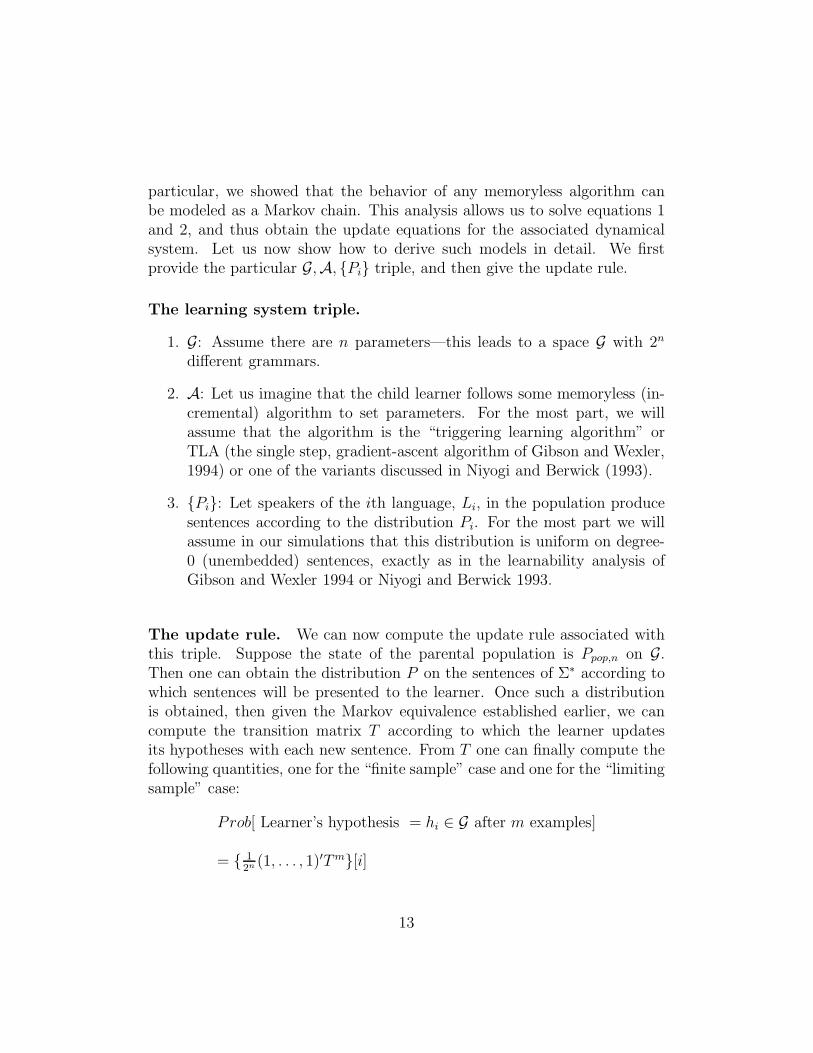
particular, we showed that the behavior of any memoryless algorithm canbe modeled as a Markov chain. This analysis allows us to solve equations 1and 2, and thus obtain the update equations for the associated dynamicalsystem. Let us now show how to derive such models in detail. We firstprovide the particular G,A, {Pi} triple, and then give the update rule.

The learning system triple.

1. G: Assume there are n parameters—this leads to a space G with 2n

different grammars.

2. A: Let us imagine that the child learner follows some memoryless (in-cremental) algorithm to set parameters. For the most part, we willassume that the algorithm is the “triggering learning algorithm” orTLA (the single step, gradient-ascent algorithm of Gibson and Wexler,1994) or one of the variants discussed in Niyogi and Berwick (1993).

3. {Pi}: Let speakers of the ith language, Li, in the population producesentences according to the distribution Pi. For the most part we willassume in our simulations that this distribution is uniform on degree-0 (unembedded) sentences, exactly as in the learnability analysis ofGibson and Wexler 1994 or Niyogi and Berwick 1993.

The update rule. We can now compute the update rule associated withthis triple. Suppose the state of the parental population is Ppop,n on G.

Then one can obtain the distribution P on the sentences of Σ∗ according towhich sentences will be presented to the learner. Once such a distributionis obtained, then given the Markov equivalence established earlier, we cancompute the transition matrix T according to which the learner updatesits hypotheses with each new sentence. From T one can finally compute thefollowing quantities, one for the “finite sample” case and one for the “limitingsample” case:

Prob[ Learner’s hypothesis = hi ∈ G after m examples]

= { 1

2n(1, . . . , 1)′Tm}[i]

13

Similary, making use of the limiting distributions of Markov chains (Resnick,1992) one can obtain the following (where ONE is a 1

2n× 1

2nmatrix with all

ones).

Prob[ Learner’s hypothesis = hi“in the limit”]

= (1, . . . , 1)′(I − T + ONE)−1

These expressions allow us to compute the linguistic composition of the pop-ulation from one generation to the next according to our analysis of theprevious section.

Remark. The limiting distribution case is more complex than the finitesample case and requires some careful explanation. There are two possibili-ties. If there is just a single target grammar, then, by definition, the learnersall identify the target correctly in the limit, and there is no further changein the linguistic composition from generation to generation. This case isessentially uninteresting. If there are two or more target grammars, thenrecalling our analysis of learnability (Niyogi and Berwick, 1994), there canbe no absorbing states in the Markov chain corresponding to the paramet-ric grammar family. In this situation, a single learner will oscillate betweensome set of states in the limit. In this sense, learners will not converge toany single, correct target grammar. However, there is a sense in which wecan characterize limiting behavior for learners: although a given learner willvisit each of these states infinitely often in the limit, it will visit some moreoften than others. The exact percentage the learner will be in a particularstate is given by equation 2.2 above. Therefore, since we know the fractionof the time the learner spends in each grammatical state in the limit, weassume that this is the probability with which it internalizes the grammarcorresponding to that state in the Markov chain.

Summarizing the basic computational framework for modeling languagechange:

1. Let π1 be the initial population mix, i.e., the percentage of differentlanguage speakers in the community. Assuming that the ith group ofspeakers produces sentences with probability Pi, we can obtain theprobability P with which sentences in Σ∗ occur for the next generationof learners.

14

2. From P we can obtain the transition matrix T for the Markov learningmodel and the limiting distribution of the linguistic composition π2 forthe next generation.

3. The second generation now has a population mix of π2. We repeat step1 and obtain π3. Continuing in this fashion, in general we can obtainπi+1 from πi.

This completes the abstract formulation of the dynamical system model.Next, we choose three specific linguistic theories and learning paradigms tomodel particular kinds of language changes, with the goal of answering thefollowing questions:

• Can we really compute all the relevant quantities to specify the dy-namical system?

• Can we evaluate the behavior (phase-space characteristics) of the re-sulting dynamical system?

• Does the dynamical system model—the formalization—shed light ondiachronic models and linguistic theories generally?

In the remainder of this article we give some concrete answers to thesequestions within the principles and parameters theory of modern linguistictheory. We turn first to the simplest possible mathematical case, that of twolanguages (grammars) fixed by a single binary parameter. We then analyze apossibly more relevant, and more complex system, with three binary param-eters Finally, to tackle a more realistic historical problem, we consider a fiveparameter system that has actually been used in other contexts to accountfor language change.

3 One Parameter Models of Language Change

Consider the following simple scenario.G : Assume that there are only two possible grammars (parameterized by oneboolean valued parameter), associated with two languages in the world, L1

and L2. (This might in fact be true in some limited linguistic contexts.)

15

P : Suppose that speakers who have internalized grammar g1 produce sen-tences with a probability distribution P1 (on the sentences of L1). Similarly,assume that speakers who have internalized grammar g2 produce sentenceswith P2 (on sentences of L2).

One can now define

a = P1[L1 ∩ L2]; 1 − a = P1[L1 \ L2]

and similarlyb = P2[L1 ∩ L2]; 1 − b = P2[L2 \ L1]

A : Assume that the learner uses a one-step, greedy, hillclimbing approachto setting target parameters. The Triggering Learning Algorithm (TLA)described earlier is one such example.N : Let the learner receive just two example sentences before maturationoccurs, i.e., after two example sentences, the learner’s current grammaticalhypothesis will be retained for the rest of its life.

Given this framework, the learnability question for this parametric sys-tem’s can be easily formulated and analyzed. Specifically, given a particulartarget grammar (gi ∈ G), and given example sentences drawn according to Pi

and presented to the learner A, one can ask whether the learner’s hypothesiswill converge to the target.

Now it is possible to characterize the behavior of the individual learnerby a Markov chain with two states, one corresponding to each grammar (seesection 2.1 above and Niyogi and Berwick, 1994). With each example thelearner moves from state to state with according to the transition probabili-ties of the chain. The transition probabilities can be calculated and dependupon the distribution with which sentences are drawn and the relative over-lap between the languages L1 and L2. In particular, if received sentencesfollow distribution P1, the transition matrix is T1. This would be the caseif the target grammar were g1. If the target grammar is g2 and sentencesreceived according to distribution P2, the transition matrix would be T2, asshown below:

T1 =

[

1 01 − a a

]

T2 =

[

b 1 − b

0 1

]

16

Let us examine T1 in order to understand the behavior of the learnerwhen g1 is the target grammar. If the learner starts out in state 1 (initialhypothesis g1), then it remains there forever. This is because every sentencethat it receives can be analyzed and the learner will never have to entertainan alternative hypothesis. Therefore the transition (1 → 1) has probability1 and the transition (1 → 2) has probability 0. If the learner starts out instate 2, then after one example sentence, the learner will remain there withprobability a—the probability that the learner will receive a sentence thatit can analyze, i.e., a sentence in L1 ∪ L2. Correspondingly, with probability1−a, the learner will receive a sentence that it cannot analyze and will haveto change its hypothesis. Thus, the transition (2 → 2) has probability a andthe transition (2 → 1) has probability 1 − a.

T1 characterizes the behavior of the learner after one example. In gen-eral, T k

1 characterizes the behavior of the learner after k examples. It maybe easily seen that as long as a < 1, the learner converges to the grammarg1 “in the limit” irrespective of its starting state. Thus the grammar g1 isGold-learnable. A similar analysis can be carried out for the case when thetarget grammar is g2. In this case, T2 describes the corresponding behaviorof the learner, and g2 is Gold-learnable if b < 1. In short the entire systemis Gold-learnable if a, b < 1—crucially assuming that maturation occurs andthe learner fixes a hypothesis forever after some N examples, with N givenin advance. Clearly, if N is very large, then the learner will, with high prob-ability, acquire the unique target grammar, whatever that grammar mightbe. At the same time, there is a finite probability that the learner will mis-converge and this will have consequences for the linguistic composition of thepopulation as discussed in the previous section. For the analysis that follows,we will assume that N = 2.

3.1 One Parameter Systems: The Linguistic Popula-tion

Continuing with our one-parameter model, we next analyze distributions overspeakers. At any given point in time, the population consists only of speakersof L1 and L2. Consequently, the linguistic composition can be representedby a single variable, p: this will denote the fraction of the population speak-ing L1. Clearly 1 − p will speak L2. Therefore this language community’s

17

composition over time can be explicitly computed as follows.

Theorem 1 The linguistic composition in the n + 1th (pn+1) generation isprovided by the following transformation on the linguistic composition of nth

generation (pn):pn+1 = Ap2

n + Bpn + C

where A = 1

2((1 − b)2 − (1 − a)2); B = b(1 − b) + (1 − a) and C = b2

2.

Proof. This is a simple specialization of the formula given in the previoussection. Details are left to the reader.

Remarks.

1. When a = b, the system has exponential growth. When a 6= b the dy-namical system is a quadratic map (which can be reduced by a transfor-mation of variables to the logistic, and shares the logistic’s dynamicalproperties). See fig. 2.

FIGURE 2 HERE

2. The scenario a 6= b—that the distributions for L1 and L2 differ—ismuch more likely to occur in the real world. Consequently, we aremore likely to see logistic growth rather than exponential ones. Indeed,various parametric shifts observed historically seem to follow an S −shaped curve. Models of these shifts have typically assumed the logisticgrowth (Kroch, 1990). Crucially, in this simple case, the logistic formhas now been derived as a conseqence of specific assumptions abouthow learning occurs at the individual level, rather than assumed , as inall previous models for language change that we are aware of.

3. We get a class of dynamical systems. The quadratic nature of ourmap comes from the fact that N = 2. If we choose other values forN we would get cubic and higher order maps. In other words, thereare already an infinite number of maps in the simple one parametercase. For larger parametric systems the mathematical situation is sig-nificantly more complex.

18

4. Logistic maps are known to be chaotic. In our system, it is possible toshow that:

Theorem 2 Due to the fact that a, b ≤ 1, the dynamical system neverenters a chaotic regime.

This observation naturally raises the question of whether nonchaoticbehavior holds for all grammatical dynamical systems, specifically thelinguistically “natural” cases. Or are there linguistic systems wherechaos will manifest itself? It would obviously be quite interesting ifall the natural grammatical spaces were nonchaotic. We leave these asopen questions.

We next turn to more linguistically plausible applications of the dynam-ical systems model. We begin with a simple 3-parameter system as our firstexample, considering variations on the learning algorithm, sentence distribu-tions, and sample size available for learning. We then consider a different,5-parameter system already presented in the literature (Clark and Roberts,1993) as one intended to partially characterize the change from Old Frenchto Modern French.

4 Example 2: A Three Parameter System

The previous section developed the necessary mathematical and computa-tional tools to completely specify the dynamical systems corresponding tomemoryless algorithms operating on finite parameter spaces. In this exam-ple we investigate the behavior of these dynamical systems. Recall that everychoice of (G,A, {Pi}) gives rise to a unique dynamical system. We start bymaking specific choices for these three elements:

1. G : This is a 3-parameter syntactic subsystem described in Gibson andWexler (1994). Thus G has exactly 8 grammars, generating languagesfrom L1 through L8, as shown in the appendix of this paper (takenfrom Gibson and Wexler, 1994).

2. A : The memoryless algorithms we consider are the TLA, and vari-ants by dropping either or both of the single-valued and greedinessconstraints.

19

3. {Pi} : For the most part, we assume sentences are produced accord-ing to a uniform distribution on the degree-0 sentences of the relevantlanguage, i.e., Pi is uniform on (degree-0 sentences of) Li.

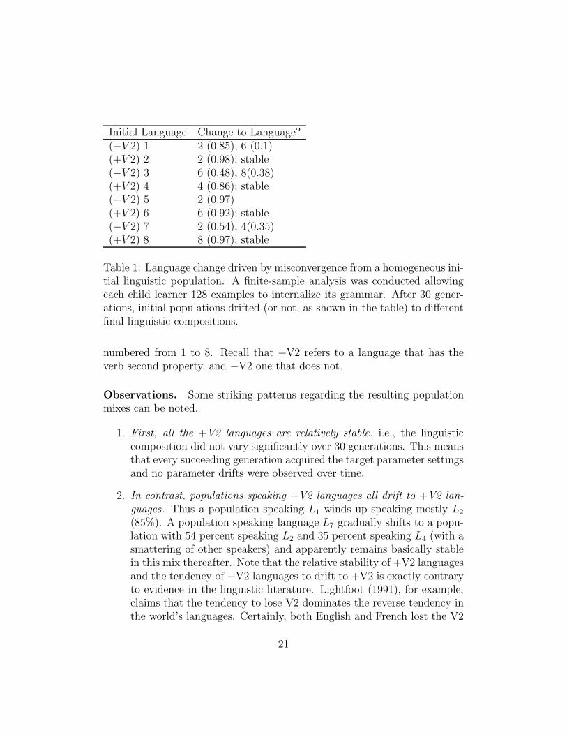
Ideally of course, a complete investigation of diachronic possibilities wouldinvolve varying G, A, and P and characterizing the resulting dynamical sys-tems by their phase space plots. Rather than explore this entire space, wefirst consider only systems evolving from homogeneous initial populations,under four basic variants of the learning algorithm A. This will give usan initial grasp of how linguistic populations can change. Indeed, linguisticchange has been studied before; even the dynamical system metaphor itselfhas been invoked. Our computational paradigm lets us say much more thanthese previous descriptions: (1) we can say precisely what the rates of changewill be; (2) we can determine what diachronic population curve changes willlook like, without stipulating in advance that they must be S-shaped (sig-moid) or not, and without curve fitting to a pre-defined functional form.

4.1 Homogeneous Initial Populations

First we consider the case of a homogeneous population—no noise or con-founding factors like foreign target languages. How stable are the languagesin the 3-parameter system in this case? To determine this, we begin with afinite-sample analysis with n = 128 example sentences (recall by the analysisof Niyogi and Berwick (1993,1994a,1994b) that learners converge to targetlanguages in the 3-parameter system with high probability after hearing thismany sentences). Some small proportion of the children misconverge; thegoal is to see whether this small proportion can drive language change—andif so, in what direction. To give the reader some idea of the possible out-comes, let us consider the four possible variations in the learning algorithm(±Single-step, ±Greedy)holding fixed the sentence distributions and learningsample.

4.1.1 Variation 1: A = TLA (+Single Step, +Greedy); Pi = Uni-form; Finite Sample = 128

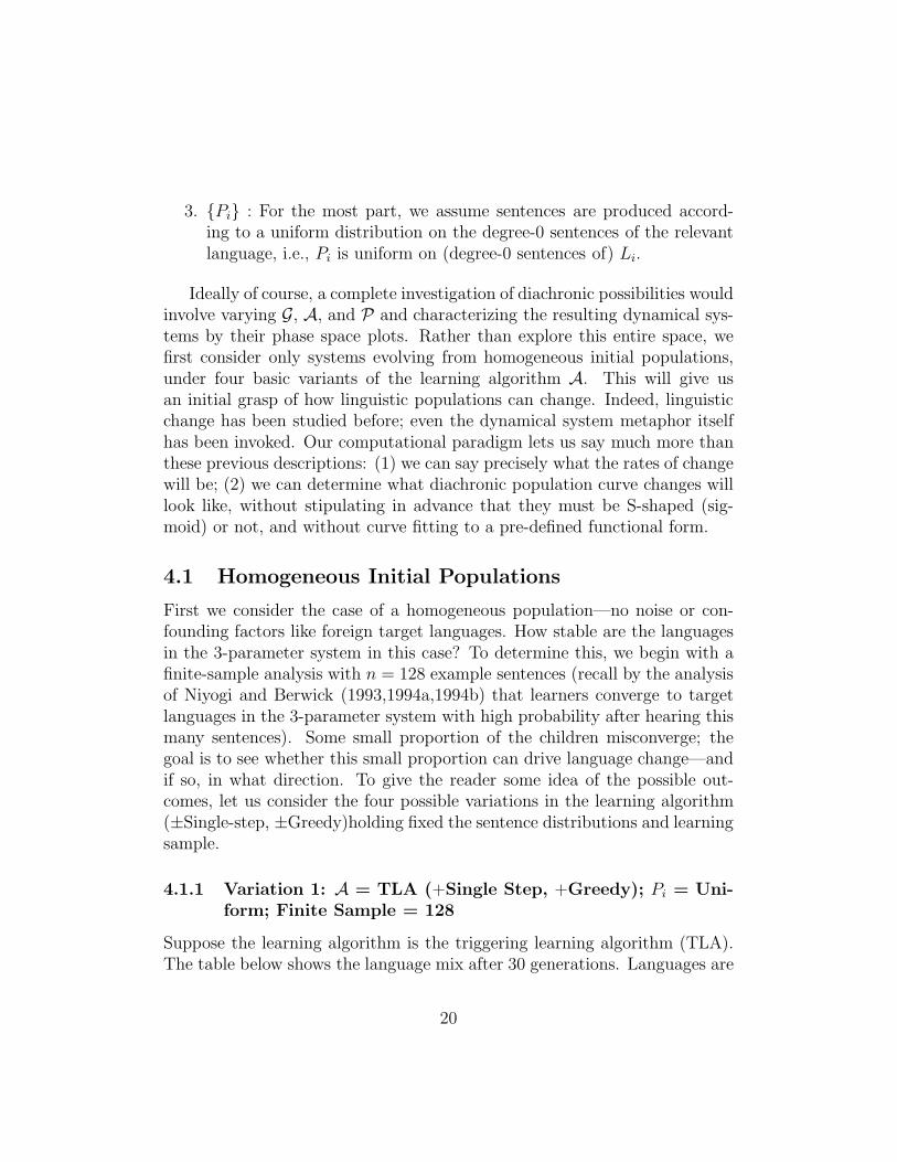
Suppose the learning algorithm is the triggering learning algorithm (TLA).The table below shows the language mix after 30 generations. Languages are

20

Initial Language Change to Language?(−V 2) 1 2 (0.85), 6 (0.1)(+V 2) 2 2 (0.98); stable(−V 2) 3 6 (0.48), 8(0.38)(+V 2) 4 4 (0.86); stable(−V 2) 5 2 (0.97)(+V 2) 6 6 (0.92); stable(−V 2) 7 2 (0.54), 4(0.35)(+V 2) 8 8 (0.97); stable

Table 1: Language change driven by misconvergence from a homogeneous ini-tial linguistic population. A finite-sample analysis was conducted allowingeach child learner 128 examples to internalize its grammar. After 30 gener-ations, initial populations drifted (or not, as shown in the table) to differentfinal linguistic compositions.

numbered from 1 to 8. Recall that +V2 refers to a language that has theverb second property, and −V2 one that does not.

Observations. Some striking patterns regarding the resulting populationmixes can be noted.

1. First, all the +V2 languages are relatively stable, i.e., the linguisticcomposition did not vary significantly over 30 generations. This meansthat every succeeding generation acquired the target parameter settingsand no parameter drifts were observed over time.

2. In contrast, populations speaking −V2 languages all drift to +V2 lan-guages. Thus a population speaking L1 winds up speaking mostly L2

(85%). A population speaking language L7 gradually shifts to a popu-lation with 54 percent speaking L2 and 35 percent speaking L4 (with asmattering of other speakers) and apparently remains basically stablein this mix thereafter. Note that the relative stability of +V2 languagesand the tendency of −V2 languages to drift to +V2 is exactly contraryto evidence in the linguistic literature. Lightfoot (1991), for example,claims that the tendency to lose V2 dominates the reverse tendency inthe world’s languages. Certainly, both English and French lost the V2

21

parameter setting—an empirically observed phenomenon that needs tobe explained. Immediately then, we see that our dynamical systemdoes not evolve in the expected manner. The reason could be due toany of the assumptions behind the model: the the parameter space, thelearning algorithm, the initial conditions, or the distributional assump-tions about sentences presented to learners. Exactly which is in errorremains to be seen, but nonetheless our example shows concretely howassumptions about a grammatical theory and learning theory can makeevolutionary, diachronic predictions—in this case, incorrect predictionsthat falsify the assumptions.

3. The rates at which the linguistic composition changes vary significantlyfrom language to language. Consider for example the change of L1 toL2. Figure 3 below shows the gradual decrease in speakers of L1 oversuccessive generations along with the increase in L2 speakers. We seethat over the first 6 or seven generations very little change occurs, butover the next 6 or seven generations the population changes at a muchfaster rate. Note that in this particular case the two languages differonly in the V2 parameter, so the curves essentially plot the gain of V2.In contrast, consider figure 4 which shows the decrease of L5 speakersand the shift to L2. Here we note a sudden change: over a space of just4 generations, the population shifts completely. Analysis of the timecourse of language change has been given some attention in linguisticanalyses of diachronic syntax change, and we return to this issue below.

FIGURE 3 HERE

FIGURE 4 HERE

4. We see that in many cases a homogeneous population splits up intodifferent linguistic groups, and seems to remain stable in that mix. Inother words, certain combinations of language speakers seem to asymp-tote towards equilibrium (at least through 30 generations). For exam-ple, a population of L7 speakers shifts over 5–6 generations to one with54 percent speaking L2 and 35 percent speaking L4 and remains thatway with no shifts in the distribution of speakers. Of course, we donot know for certain whether this is really a stable mixture. It could

22

be that the population mix could suddenly shift after another 100 gen-erations. What we really need to do is characterize the stable pointsor “limit cycles” of these dynamical systems. Other linguistic mixescan be inherently unstable; they might drift systematically to stablesituations, or might shift dramatically (as with language L1).

5. It seems that the observed instability and drifts are to a large extent anartifact of the learning algorithm. Remember that the TLA suffers fromthe problem of local maxima.12 We note that those languages whoseacquisition is not impeded by local maxima (the +V2 languages) arestable over time. Languages that have local maxima are unstable; inparticular they drift to the local maxima over time. Consider L7. Ifthis is the target language, then there are two local maxima (L2 andL4) and these are precisely the states to which the system drifts overtime. The same is true for languages L5 and L3. In this respect, thebehavior of L1 is quite unusual since it actually does not have any localmaxima, yet it tends to flip the V2 parameter over time.

Now let us consider a different learning algorithm from the TLA thatdoes not suffer from local maxima problems, to see whether this changes thedynamical system results.

4.1.2 Variation 2: A = +Greedy, −Single value; Pi = Uniform;Finite Sample = 128

Consider a simple variant of the TLA obtained by dropping the single valuedconstraint. This implies that the learner is no longer constrained to changejust one parameter at a time: on being presented with a sentence it cannotanalyze, it chooses any of the alternative grammars and attempts to analyzethe sentence with it. Greediness is retained; thus the learner retains its orig-inal hypothesis if the new one is also not able to analyze the sentence. Giventhis new learning algorithm, and retaining all the other original assumptions,Table 2 shows the distribution of speakers after 30 generations.

12We regard local maxima of a language Li to be alternative absorbing states (sinks)in the Markov chain for that target language. This formulation differs slightly from theconception of local maxima in Gibson and Wexler (1994), a matter discussed at somelength in Niyogi and Berwick (1993). Thus according to our definition L4 is not a localmaxima for L5 and consequently no shift is observed.

23

Initial Language Change to Language?−V 2 1 2 (0.41), 4 (0.19), 6 (0.18), 8 (0.13)+V 2 2 2 (0.42), 4 (0.19), 6 (0.17), 8 (0.12)−V 2 3 2 (0.40), 4 (0.19), 6 (0.18), 8 (0.13)+V 2 4 2 (0.41), 4 (0.19), 6 (0.18), 8 (0.13)−V 2 5 2 (0.40), 4 (0.19), 6 (0.18), 8 (0.13)+V 2 6 2 (0.40), 4 (0.19), 6 (0.18), 8 (0.13)−V 2 7 2 (0.40), 4 (0.19), 6 (0.18), 8 (0.13)+V 2 8 2 (0.40), 4 (0.19), 6 (0.18), 8 (0.13)

Table 2: Language change driven by misconvergence. A finite-sample analy-sis was conducted allowing each child learner (following the TLA with single-value dropped) 128 examples to internalize its grammar. Initial populationswere linguistically homogeneous, and they drifted to different linguistic com-positions. The major language groups after 30 generations have been listedin this table. Note how all initially homogeneous populations tend to thesame composition.

Observations. In this situation there are no local maxima, and the evo-lutionary pattern takes on a very different nature. There are two distinctobservations to be made.

1. All homogeneous populations eventually drift to a strikingly similar pop-ulation mix, irrespective of what language they start from. What isunique about this mix? Is it a stable point (or attractor)? Furthersimulations and theoretical analyses are needed to resolve this ques-tion; we leave these as open questions.

2. All homogeneous populations drift to a population mix of only +V2languages. Thus, the V2 parameter is gradually set over succeedinggenerations by all people in the community (irrespective of which lan-guage they speak). In other words, as before, there is a tendency togain V2 rather than lose V2, contrary to the empirical facts.

As an example, fig. 5 shows the changing percentage of the populationspeaking the different languages starting off from a homogeneous populationspeaking L5. As before, learners who have not converged to the target in 128

24

Initial Language Change to Language?Any Language 1 (0.11), 2 (0.16), 3 (0.10), 4 (0.14)(Homogeneous) 5 (0.12), 6 (0.14), 7 (0.10), 8 (0.13)

Table 3: Language change driven by misconvergence, using two differentacquisition algorithms that do not obey a local gradient-ascent rule (a greed-iness constraint). A finite-sample analysis was conducted with the learningalgorithm following a random-step algorithm or else a single-step algorithm,along with 128 examples to internalize its grammar. Initial populations werelinguistically homogeneous, and they drifted to different linguistic composi-tions. The major language groups after 30 generations have been listed inthis table. Note that all initially homogeneous populations converge to thesame final composition.

examples are the driving force for change here. Note again the time evolutionof the grammars. For about 5 generations there is only a slight decrease inthe percentage of speakers of L5. Then the linguistic patterns switch rapidlyover the next 7 generations to a relatively stable mix.

FIGURE 5 HERE

4.1.3 Variations 3 & 4: −Greedy, ±Single Value constraint; Pi

=Uniform; Finite Sample = 128

Having dropped the single value constraint, we consider the next obviousvariation in the learning algorithm: dropping greediness while varying thesingle value constraint. Again, our goal is to see whether this makes anydifference in the resulting dynamical system. This gives rise to two differentlearning algorithms: (1) allow the learning algorithm to pick any new gram-mar at most one parameter value away from its current hypothesis (retainingthe single-value constraint, but without greediness, that is, the new grammardoes not have to be able to parse the current input sentence); (2) allow thelearning algorithm to pick any new grammar at each step (no matter howfar away from its current hypothesis).

In both cases, the population mix after 30 generations is the same irre-spective of the initial language of the homogeneous population. These resultsare shown in table 3.

25

Observations:

1. Both algorithms yield dynamical systems that arrive at the same popu-lation mix after 30 generations. The path by which they arrive at thismix is, however, not the same (see figure 6).

2. The final population mix contains all languages in significant propor-tion. This is in distinct contrast to the previous situations, where wesaw that −V2 languages were eliminated over time.

FIGURE 6 HERE

4.2 Modeling Diachronic Trajectories

With a basic notion of how diachronic systems can evolve given differentlearning algorithms, we turn next to the question of population trajecto-ries. While we can already see that some evolutionary trajectories have a“linguistically classical” S-shape, their smoothness can vary. However, ourformalization allows us to say much more than this. Unlike the previous workin diachronic linguistics that we are familiar with, we can explore the spaceof possible trajectories, examining factors that affect their evolutionary timecourse, without assuming an a priori S-shape.

For example, Bailey (1973) proposed a “wave” model of linguistic change:linguistic replacements follow an S-shaped curve over time. In Bailey’s ownwords (taken from Kroch, 1990):

A given change begins quite gradually; after reaching a certainpoint (say, twenty percent), it picks up momentum and proceedsat a much faster rate; and finally tails off slowly before reachingcompletion. The result is an S-curve: the statistical differencesamong isolects in the middle relative times of the change will begreater than the statistical differences among the early and lateisolects.

The idea that linguistic changes follow an S-curve has also been proposedby Osgood and Sebeok (1954) and Weinreich, Labov, and Herzog (1968).More specific logistic forms have been advanced by Altmann (1983) andKroch (1982,1989). Here, the idea of a logistic functional form is borrowed

26

from population biology where it is demonstrable that the logistic governsthe replacement of organisms and of genetic alleles that differ in Darwinianfitness. However, Kroch (1989) concedes that “unlike in the population biol-ogy case, no mechanism of change has been proposed from which the logisticform can be deduced.”

Crucially, in our case, we suggest a specific mechanism of change: anacquisition-based model where the combination of grammatical theory, learn-ing algorithms, and distributional assumptions on sentences drive change.The specific form might or might not be S-shaped, and might have varyingrates of change.13

Among the other factors that affect evolutionary trajectories are matu-ration time—the number of sentences available to the learner before it inter-nalizes its adult grammar—and the distributions with which sentences arepresented to the learner. We examine these in turn.

4.2.1 The Effect of Maturation Time or Sample Size

One obvious factor influencing the evolutionary trajectories is the matura-tional time, i.e., the number (N) of sentences the child is allowed to hearbefore forming its mature hypothesis. This was fixed at 128 in all the sys-tems shown so far (based in part on our explicit computation for the Markovconvergence time in this situation). Figure 7 shows the effect of varying N onthe evolutionary trajectories. As usual, we plot only a subspace of the popu-lation. In particular, we plot the percentage of L2 speakers in the populationwith each succeeding generation. The initial composition of the populationwas homogeneous (with people speaking L1).

Observations.

13Of course, we do not mean to say that we can simulate any possible trajectory—thatwould make the formalism empty. Rather, we are exploring the initial space of possibletrajectories, given some example initial conditions that have been already advanced in theliterature. Because the mathematics for dynamical systems is in general quite complex,at present we cannot make general statements of the form, “under these particular initialconditions the trajectory will be sigmoidal, and under these other conditions it will not be.”We have conducted only very preliminary investigations demonstrating that potentially atleast, reasonable, distinct initial conditions can lead to demonstrably different trajectories.

27

1. The initial rate of change of the population is highest when the matu-ration time is smallest , i.e., the learner is allowed the least amount oftime to develop its mature hypothesis. This is not surprising. If thelearner were allowed access to a lot of examples to make its maturehypothesis, most learners would reach the target grammar. Very fewwould misconverge, and the linguistic composition would change littleover the next generation. On the other hand, if the learner were allowedvery few examples to develop its hypothesis, many would misconverge,possibly causing great change over one generation.

2. The “stable” linguistic compositions seem to depend upon maturationtime. For example, if learners are allowed only 8 examples, the per-centage of L2 speakers rises quickly to about 0.26. On the other hand,if learners are allowed 128 examples, the percentage of L2 speakerseventually rises to about 0.41.

3. Note that the trajectories do not have an S-shaped curve in contrastto the results of Kroch (1989).

4. The maturation time is related to the order of the dynamical system.

FIGURE 7 HERE

4.2.2 The Effect of Sentence Distributions (Pi)

Another important factor influencing evolutionary trajectories is the distri-bution Pi with which sentences of the ith language, Li, are presented to thelearner. In a certain sense, the grammatical space and the learning algo-rithm jointly determine the order of the dynamical system. On the otherhand, sentence distributions are much like the parameters of the dynami-cal system (see sec. 4.3.2). Clearly the sentence distributions affect rates ofconvergence within one generation. Further, by putting greater weight oncertain word forms rather than others, they might influence systemic evolu-tion in certain directions. While this is again an obvious point, the modellets us consider the alternatives precisely.

To illustrate the idea, consider the following example: the interactionbetween L1 and L2 speakers in the community as the sentence distributionswith which these speakers produce sentences changes. Recall that so far

28

we have assumed that all speakers produce sentences with uniform distribu-tions on degree-0 sentences of their respective languages. Now we consideralternative distributions, parameterized by a value p:

1. Let L1,2 = L1 ∩ L2.

2. P1 : Speakers of L1 produce sentences so that all degree-0 sentences ofL1,2 are equally likely and their total probability is p. Further, sentencesof L1 \ L1,2 are also equally likely, but their total proability is 1 − p.

3. P2 : Speakers of L2 produce sentences so that all degree-0 sentences ofL1,2 are equally likely and their total probability is p. Further, sentencesof L2 \ L1,2 are also equally likely, but their total proability is 1 − p.

4. Other Pi’s are all uniform over degree-0 sentences.

The parameter p determines the weight on the sentence patterns in com-mon between the languages L1 and L2. Figure 8 shows the evolution of the L2

speakers as p varies. Here the learning algorithm is +Greedy, +Single value(TLA, or local gradient ascent) and the initial population is homogeneous,100% L1; 0% L2. Note that the system moves in different ways as p varies.When p is very small (0.05), that is, sentences common to L1 and L2 occurinfrequently, in the long run the percentage of L2 speakers does not increase;the population stays put with L1. However, as p grows, more strings of L2

occur, and the dynamical system changes so that the long-term percentageof L1 speakers decreases and that of L2 speakers increases. When p reaches0.75 the initial population evolves into a completely L2 speaking commu-nity. After this, as p increases further, we notice (see p = 0.95) that the L2

speakers increase but can never rise to 100 percent of the population; thereis still a residual L1 speaking component. This is to be expected, because forsuch high values of p, many strings common to L1 and L2 occur frequently.This means that a learner could sometimes converge to L1 just as well as L2,and some learners indeed begin to do so, increasing the number of the L1

speakers.This example shows us that if we wanted a homogeneous L1 speaking pop-

ulation to move to a homogeneous L2 speaking population, by choosing ourdistributions appropriately, we could drive the grammatical dynamical sys-tem in the appropriate direction. It suggests another important application

29

of the dynamical system approach: one can work backwards, and examinethe conditions needed to generate a change of a certain kind. By checkingwhether such conditions could have possibly existed historically, we can fal-sify a grammatical theory or a learning paradigm. Note that this exampleshowed the effect of sentence distributions, and how to alter them to obtaindesired evolutionary envelopes. One could, in principle, alter the grammati-cal theory or the learning algorithm in the same fashion—-leading to a toolto aid the search for an adequate linguistic theory.14

FIGURE 8 HERE

4.3 Nonhomogeneous Populations: Phase-Space Plots

For our three-parameter system, we have been able to characterize the up-date rules for the dynamical systems corresponding to a variety of learningalgorithms. Each dynamical system has a specific update procedure accord-ing to which the states evolve from some homogeneous initial population. Amore complete characterization of the dynamical system would be achievedby obtaining phase-space plots of this system. Such phase-space plots arepictures of the state-space S filled with trajectories obtained by letting thesystem evolve from various initial points (states) in the state space.

4.3.1 Phase-Space Plots: Grammatical Trajectories

We have described earlier the relationship between the state of the populationin one generation and the next. In our case, let Π denote an 8-dimensionalvector variable (state variable). Specifically, Π = (π1, . . . , π8)

′ (with∑8

i=1 πi)as we discussed before. The following schema reiterates the chain of depen-dencies involved in the update rule governing system evolution. The state ofthe population at time t (in generations), allows us to compute the transi-tion matrix T for the Markov chain associated with the memoryless learner.Now, depending upon whether we want (1) an asymptotic analysis or (2) afinite sample analysis, we compute (1) the limiting behavior of Tm as m (thenumber of examples) goes to infinity (for an asymptotic analysis), or (2) the

14Again, we stress that we obviously do not want so weak a theory that we can arrive atany possible initial conditions simply by carrying out reasonable changes to the sentencedistributions. This may, of course, be possible; we have not yet examined the general case.

30

value of TN (where N is the number of examples after which maturationoccurs). This allows us to compute the next state of the population. ThusΠ(t + 1) = g(Π(t)) where g is a complex non-linear relation.

Π(t) =⇒ P on Σ∗ =⇒ T =⇒ Tm =⇒ Π(t + 1)

If we choose a certain initial condition Π1, the system will evolve according tothe above relation and one can obtain a trajectory of Π in the 8 dimensionalspace over time. Each initial condition yields a unique trajectory and onecan then plot these trajectories obtaining a phase-space plot. Each suchtrajectory corresponds to a line in the 8-dimensional plane given by

∑

8i=1 πi =

1. One cannot directly display such a high dimensional object, but we plotin figure 9 the projection of a particular trajectory onto a two dimensionalsubspace given by (π1(t), π2(t)) (the proportion of speakers of L1 and L2) atdifferent points in time.

FIGURE 9 HERE

As mentioned earlier, with a different initial condition we get a differ-ent grammatical trajectory. The complete state space picture is thus filledwith all the different trajectories corresponding to different initial conditions.Fig. 10 shows this.

FIGURE 10 HERE

4.3.2 Stability Issues

The phase-space plots show that many initial conditions yield trajectoriesthat seem to converge to a single point in the state space. In the dynami-cal systems terminology, this corresponds to a fixed point of the system—apopulation mix that stays at the same composition. Many natural questionsarise at this stage. What are the conditions for stability? How many fixedpoints are there in a given system? How can we solve for them? These areinteresting questions but detailed answers are not within the scope of thecurrent paper. In lieu of a more complete analysis we merely state here theequations that allow one to characterize the stable population mixes.

First, some notational preliminaries. As before, let Pi be the distributionon the sentences of the ith language Li. From Pi, we can construct Ti, the

31

transition matrix whose elements are given by the explicit procedure docu-mented in Niyogi and Berwick (1993, 1994a, 1994b). The matrix Ti modelsa +Greedy −Single value learner if the target language is Li (with sentencesfrom the target produced with Pi). Similarly, one can obtain the matrices forother learning variants. Note that fixing the Pi’s fixes the Ti’s and in so thePi’s are a different sort of “parameter” that characterize how the dynamicalsystem evolves.15 If the state of the parent population at time t is Π(t), thenit is possible to show that the (true) transition matrix for ±Greedy ±Singlevalue learners is T =

∑8i=1 πi(t)Ti. For the finite case analysis, the following

holds

Statement 1 (Finite Case) A fixed point (stable point) of the grammaticaldynamical system (obtained by a ±Greedy ±Single value learner operatingon the 8 parameter space with k examples to choose its final hypothesis) is asolution of the following equation:

Π′ = (π1, . . . , π8) = (1, . . . , 1)′(8

∑

i=1

πiTi)k

Note: This equation is obtained simply by setting Π(t + 1) = Π(t). Notehowever, that this is an example of a nonlinear multidimensional iteratedfunction map. The analysis of such dynamical systems is nontrivial, and ourtheorem by no means captures all the possibilities.

Similarly, for the limiting (asymptotic) case, the following holds:

Statement 2 (Limiting or Asymptotic Analysis) A fixed point (stablepoint) of the grammatical dynamical system (obtained by a ±Greedy ±Singlevalue learner operating on the 8 parameter space (given infinite examples tochoose its mature hypothesis) is a solution of the following equation:

Π′ = (π1, . . . , π8) = (1, . . . , 1)′(I −8

∑

i=1

πiTi + ONE)−1

where ONE is the 8 × 8 matrix with all its entries equal to 1.

15There are thus two distinct kinds of parameters in our model: first, parameters thatdefine the 2n languages and define the state-space of the system; and second, the Pi’s thecharacterize the way in which the system evolves and are therefore the parameters of thecomplete grammatical dynamical system.

32

Note: Again this is trivially obtained by setting Π(t+1) = Π(t). The expres-sion on the right provides an analytical expression for the update equationin the asymptotic case. See Resnick (1992) for details. All the caveats men-tioned before in the Finite case statement apply here as well.

Remark. We have just touched the surface as far as the theoretical char-acterization of these grammatical dynamical systems are concerned. Themain purpose of this paper is to show that these dynamical systems existas a logical consequence of assumptions about the grammatical space andan acquisition theory. We have exhibited only some preliminary simulationswith these systems. From a theoretical perspective, it would be much morevaluable to have complete characterizations of such systems. Strogatz (1993)suggests that nonlinear multidimensional mappings with greater than 3 di-mensions are likely to be chaotic. It is also interesting to note that iteratedfunction maps define fractal sets . Such investigations are beyond the scopeof this paper, and might well be a fruitful area for further research.

5 Example 2: From Old French to Modern

French; Clark and Roberts’ Analysis Re-

visited

So far, our examples have been based on a 3-parameter linguistic theory forwhich we derived several different dynamical systems. Our goal was to con-cretely instantiate our philosophical arguments, sketching the factors thatinfluence evolutionary trajectories. In this section, we briefly consider a dif-ferent parametric linguistic system studied by Clark and Roberts, 1993. Thehistorical context in which Clark and Roberts advanced their linguistic pro-posal is the evolution of Modern French from Old French. Their parametersare intended to capture some, but of course not all, of this change. They toouse a learning algorithm—in their case, a genetic algorithm—to account forhistorical change but do not analyze their model from the dynamical systemsviewpoint. Here we adopt their parameterization, with all its strengths andweaknesses, but consider an alternative learning paradigm and the dynamicalsystems approach.

33

Extensive simulations in the earlier section reveal that while the learnabil-ity problem of the 3-parameter space can be solved by stochastic hill climbingalgorithms, the long term evolution of these algorithms have a behavior thatis at variance with the diachronic change actually observed in historical lin-guistics. In particular, we saw how there was a tendency to gain rather thanlose the V2 parameter setting. While this could well be an artifact of theclass of learning algorithms considered, a more likely explanation is that lossof V2 (observed in many of the world’s languages like French, English, andso forth) is due to an interaction of parameters and triggers other than thoseconsidered in the previous section. We investigate this possibility and beginby first reviewing Clark and Roberts’ alternative parametric theory.

5.1 The Parametric Subspace and Data

We now consider a syntactic space involving the with 5 (boolean-valued)parameters. We do not attempt to describe these parameters. The interestedreader should consult Haegeman (1991) for details and Clark and Roberts(1993) for details.

1. p1: Case assignment under agreement (p1 = 1) or not (p1 = 0).

2. p2: Case assignment under government (p2 = 1) or not ((p2 = 0).Relevant triggers for this parameter include “Adv V S”, “S V O”.

3. p3: Nominative clitics.

4. p4: Null Subject. Here relevant triggers would include “wh V S O”.

5. p5: Verb-second V2. Triggers include “Adv V S” , and “S V O”.

These 5 parameters define a 32 grammar space. Each grammar in thisparametrized system can be represented by a string of 5 bits depending uponthe values of p1, . . . , p5, for instance, the first bit position corresponds tocase assignment under agreement. We can now look at the surface strings(sentences) generated by each such grammar. For the purpose of explaininghow Old French changed to Modern French, Clark and Roberts consider thefollowing key sentences. The parameter settings required to generate eachsentence are provided in brackets; an asterisk is a “doesn’t matter” value andan “X” means any phrase.

34

The Relevant Data

adv V S [*1**1]SVO [*1**1] or [1***0]wh V S O [*1***]wh V S O [**1**]X (pro) V O [*1*11] or [1**10]X V s [**1*1]X s V [**1*0]X S V [1***0](S) V Y [*1*11]

The parameter settings provided in brackets set the grammars which gen-erate the sentence. For example, the sentence form “adv V S” (correspondingto quickly ran John), an incorrect word order in English) is generated by allgrammars that have case assignment under government (the second elementof the array set to 1, p2 = 1) and verb second movement (p5 = 1). The otherparameters can be set to any value. Clearly there are 8 different grammarsthat can generate (alternatively parse) this sentence. Similarly there are 16grammars that generate the form S V O (8 corresponding to parameter set-tings of [*1**1] and 8 corresponding to parameter settings of [1***0]) and 4grammars that generate ((s) V Y).

Remark. Note that the sentence set Clark and Roberts considered is onlya subset of the the total number of degree-0 sentences generated by the 32grammars in question. In order to directly compare their model with ours, wehave not attempted to expand the data set or fill out the space any further.As a result, all the grammars do not have unique extensional properties, i.e.,some generate the same set of sentences.

5.2 The Case of Diachronic Syntax Change in French

Continuing with Clark and Roberts’ analysis, within this parameter space,it is historically observed that the language spoken in France underwent aparametric change from the twelfth century to modern times. In particular,they point out that both V2 and prodrop are lost, illustrated by exampleslike these:Loss of null subjects: pro-drop

35

(1) (Old French; +pro drop)Si firent (pro) grant joie la nuit‘thus (they) made great joy the night’

(2) (Modern French; −pro drop)∗Ainsi s’amusaient bien cette nuit

‘thus (they) had fun that night’

Loss of V2

(3) (Old French; +V2)Lors oirent ils venir un escoiz de tonoire‘then they heard come a clap of thunder’

(4) (Modern French; −V2)∗Puis entendirent-ils un coup de tonerre. ‘then they heard a clap of

thunder’

Clark and Roberts observe that it has been argued this transition wasbrought about by the introduction of new word orders during the fifteenthand sixteenth centuries resulting in generations of children acquiring slightlydifferent grammars and eventually culminating in the grammar of modernFrench. A brief reconstruction of the historical process (after Clark andRoberts, 1993) runs as follows.Old French; setting [11011] The language spoken in the twelfth and thir-teenth centuries had verb-second movement and null subjects, both of whichwere dropped by the twentieth century. The sentences generated by theparameter settings corresponding to Old French are:

Old Frenchadv V S – [*1**1]S V O – [*1**1] or [1***0]wh V S O [*1***]X (pro) V O [*1*11] or [1**10]

Note that from this data set it appears that both the Case agreementand nominative clitics parameters remain ambiguous. In particular, OldFrench is in a subset-superset relation with another language (generated bythe parameter settings of 11111). In this case, possibly some kind of subset

36

principle (Berwick, 1985) could be used by the learner; otherwise it is notclear how the data would allow the learner to converge to the Old Frenchgrammar in the first place. None of the ±Greedy, ±Single value algorithmswould converge uniquely to the grammar of Old French.

The string (X)VS occurs with frequency 58% and SV(X) occurs with 34%in Old French texts. I t is argued that this frequency of (X)VS is high enoughto cause the V2 parameter to trigger to +V2.Middle French In Middle French, the data is not consistent with any ofthe 32 target grammars (equivalent to a heterogenous population). Anal-ysis of texts from that period reveal that some old forms (like Adv V S)decreased in frequency and new forms (like Adv S V) increased. It is arguedin Clark and Roberts that such a frequency shift causes ”erosion” of V2,brings about parameter instability and ultimately convergence to the gram-mar of Modern French. In this transition period (i.e. when Middle Frenchwas spoken/written) the data is of the following form:

adv V S [*1**1]; SVO [*1**1] or [1***0]; wh V S O [*1***]; wh V s O[**1**]; X (pro)V O [*1*11] or [1**10]; X V s [**1*1]; X s V [**1*0]; X S V[1***0]; (s)VY [*1*11]

Thus, we have old sentence patterns like Adv V S (though it decreasesin frequency and becomes only 10%), SVO, X (pro)V O and whVSO. Thenew sentence patterns which emerge at this stage are adv S V (increasesin frequency to become 60%), X subjclitic V, V subjclitic (pro)V Y (nullsubjects) , whV subjclitic O.Modern French [10100] By the eighteenth century, French had lost boththe V2 parameter setting as well as the null subject parameter setting. Thesentence patterns consistent with Modern French parameter settings are SVO[*1**1] or [1***0], X S V [1***0], V s O [**1**]. Note that this data, thoughconsistent with Modern French, will not trigger all the parameter settings.In this sense, Modern French (just like Old French) is not uniquely learnablefrom data. However, as before, we shall not concern ourselves overly withthis, for the relevant parameters (V2 and null subject) are uniquely set bythe data here.

5.3 Some Dynamical System Simulations

We can obtain dynamical systems for this parametric space, for a TLA (orTLA-like) algorithm in a straightforward fashion. We show the results of two

37

simulations conducted with such dynamical systems.

5.3.1 Homogeneous Populations [Initial–Old French]

We conducted a simulation on this new parameter space using the TriggeringLearning Algorithm. Recall that the relevant Markov chain in this case has 32states. We start the simulation with a homogeneous population speaking OldFrench (parameter setting = 11011). Our goal was to see if misconvergencealone, could drive Old French to Modern French.

Just as before, we can observe the linguistic composition of the populationover several generations. It is observed that in one generation, 15 percent ofthe children converge to grammar 01011; 18 percent to grammar 01111; 33percent to grammar 11011 (target) and 26 percent to grammar 11111 withvery few having converged to other grammars. Thereafter, the populationconsists mostly of speakers of these 4 languages, with one important differ-ence: 15 percent of the speakers eventually lose V2. In particular, they haveacquired the grammar 11110. Shown in fig. 11 are the percentage of thepopulation speaking the 4 languages mentioned above as they evolve over 20generations. Notice that in the space of a few generations, the speakers of11011, and 01011 have dropped out altogether. Most of the population nowspeaks language 1111 (46 percent) and 01111 (27 percent). Fifteen percentof the population speaks 11110 and there is a smattering of other speakers.The population remains roughly stable in this configuration thereafter.

FIGURE 11 HERE

Observations:1. On examining the four languages to which the system converges after

one generation, we noice that they share the same settings for the principles[Case assignemnt under government], [pro drop], and [V2]. These correspondto the three parameters which are uniquely set by data from Old French. Theother two parameters can take on any value. Consequently 4 languages aregenerated all of which satisfy the data from Old French.

2. Recall our earlier remark that due to insufficient data, there wereequivalent grammars in the parameter system. It turns out that in thisparticular case, the grammars (01011) and (11011) are identical as far astheir extensional properties are concerned; as are the grammars (11111) and(01111).

38

3. There is subset relation between the two sets described in (2). Thegrammar (11011) is in a subset relation with (11111). This explains whyafter a few generations most of the population switches to either (11111) or(01111) (the superset grammars).

4. An interesting feature of the simulation is that 15 percent of thepopulation eventually acquires the grammar (11110), i.e., they have lost theV2 parameter setting. This is the first sign of instability of V2 that we haveseen in our simulations so far (for greedy algorithms which are psychologicallypreferred). Recall that for such algorithms, the V2 parameter was very stablein our previous example.

5.3.2 Heterogenous Populations (Mixtures)

The earlier section showed that with no new (foreign) sentence patterns thegrammatical system starting out with only Old French speakers showed sometendency to lose V2. However, the grammatical trajectory did not terminatein Modern French. In order to more closely duplicate this historically ob-served trajectory, we examine alternative inital conditions. We start oursimulations with an initial condition which is a mixture of two sources; datafrom Old French and data from New French (reproducing in this sense, datasimilar to that obtained from the Middle French period). Thus children inthe next generation observe new surface forms. Most of the surface formsobserved in Middle French are covered by this mixture.Observations:

1. On performing the simulations using the TLA as a learning algorithmon this parameter space, an interesting pattern is observed. Suppose thelearner is exposed to sentences with 90 percent generated by Old Frenchgrammar (11011) and 10 percent by Modern French grammar (10100), withinone generation 22 percent of the learners have converged to the grammar(11110) and 78 percent to the grammar (11111). Thus the learners set eachof the parameter values to 1 except the V2 parameter setting. Now ModernFrench is a non-V2 language; and 10 percent of data from Modern French issufficient to cause 22 percent of the speakers to lose V2. This is the behaviourover one generation. The new population (consisting of 78 percent speakinggrammar (11111) and 22 percent speaking grammar (11110)) remains stablefor ever.

2. Fig. 12 shows the proportion of speakers who have lost V2 after one

39

generation, as a function of the proportion of sentences from the ModernFrench Source. The shape of the curve is interesting. For small values ofthe proportion of the Modern French source, the slope of the curve is greaterthan 1. Thus there is a greater tendency of speakers to lose V2 than toretain it. Thus 10 percent of novel sentences from the Modern French sourcecauses 20 percent of the population to lose V2; similarly 20 percent of novelsentences from the Modern French source causes 40 percent of the speakersto lose V2. This effect wears off later. This seems to capture computationallythe intuitive notion of many linguists that a small change in inputs providedto children could drive the system towards larger change.

FIGURE 12 HERE

3. Unfortunately, there are several shortcomings of this particular sim-ulation. First, we notice that mixing Old and Modern French sources doesnot cause the desired (historically observed) grammatical trajectory fromOld to Modern French (corresponding in our system to movement from state(11011) to state (10100) in our Markov Chain). Although we find that asmall injection of sentences from Modern French causes a larger percentageof the population to lose V2 and gain subject clitics (which are historicallyobserved phenomena), nevertheless, the entire population retains the nullsubject setting and case assignment under government. It should be men-tioned that Clark and Roberts argue that the change in case assignmentunder government is the driving force which allows alternate parse-trees tobe formed and causes the parametric loss of V2 and null subject. In thissense, it is a more fundamental change.

4. If the dynamical system is allowed to evolve, it ends up in eitherof the two states (11111) or (11110). This is essentially due to the subsetrelations these states (languages) have with other languages in the system.Another complication in the system is the equivalence of several differentgrammars (with respect to their surface extensions) e.g. given the data weare considering, the grammars (01011) and (11011) (Old French) generate thesame sentences. This leads to multiplicity of paths, convergence to more thanone target grammar and general inelegance of the state-space description.Future Directions: There are several possibilities to consider here.

1. Using more data and filling out the state-space might yield greaterinsight. Note that we can also study the development of other languages likeItalian or Spanish within this framework and that might be useful.

40

2. TLA-like hill climbing algorithms do not pay attention to the subsetprinciple explicitly. It would be interesting to explicitly program this intothe learning algorithm and observe the evolution thereafter.

3. There are often cases when several different grammars generate thesame sentences or atleast equally well fit the data. Algorithms which lookonly at surface strings are unable then to distinguish between them resultingin convergence to all of them with different probabilities in our stochasticsetting. We saw an example of this for convergence to four states earlier.Clark and Roberts suggest an elegance criterion by looking at the parse-trees to decide between these grammars. This difference between stronggenerative capacity and weak generative capacity can easily be incorporatedinto the Markov model as well. The transition probabilites, now, will notdepend upon the surface properties of the grammars alone, but also uponthe elegance of derivation for each surface string.

4. Rather than the evolution of the population, one could look at theevolution of the distribution of words. One can also obtain bounds on fre-quencies with which the new data in the Middle French Period must occurso that the correct drift is observed.

6 Conclusions and Directions for Future Re-

search

In this paper, we have argued that any combination of (grammatical theory,learning paradigm) leads to a model of grammatical evolution and diachronicchange. A learning theory (paradigm) attempts to account for how children(the individual child) solve the problem of language acquisition. By consid-ering a population of such “child learners”, we have arrived at a model of theemergent, global, population behavior. The key point is that such a model isa logical consequence of grammatical, and learning theories. Consequently,whenever a linguist suggests a new grammatical, or learning theory, they arealso suggesting a particular evolutionary theory—and the consequences ofthis need to be examined.

41

Historical Linguistics and Diachronic Criteria

From a programmatic persepective, this paper has two important conse-quences. First, it allows us to take a formal, analytic view of historicallinguistics. Most accounts of language change have tended to be descriptivein nature. In contrast, we place the study of historical or diachronic lin-guistics in a formal framework. In this sense, our conception of historicallinguistics is closest in spirit to evolutionary theory and population biology16

Second, this approach allows us to formally pose a diachronic criterion forthe adequacy of grammatical theories. A significant body of work in learn-ing theory, has already sharpened the learnability criterion for grammaticaltheories—in other words, the class of grammars G must be learnable by somepsychologically plausible algorithm from primary linguistic data. Now we cango one step further. The class of grammars G (along with a proposed learningalgorithm A) can be reduced to a dynamical system whose evolution mustmatch that of the true evolution of human languages (as reconstructed fromhistorical data).

We have attempted to lay the framework for the development of researchtools to study historical phenomena. To concretely demonstrate that thegrammatical dynamical systems need not be impossibly difficult to compute(or simulate), we explicitly showed how to transform parametrized theories,and memoryless learning algorithms to dynamical systems. The specific sim-ulations of this paper are far too incomplete to have any long term linguisticimplications, though, we hope, it certainly forms a starting point for re-search in this direction. Nevertheless, there were certain interesting resultsobtained.

1. We saw that the V2 parameter was more stable in the 3-parametercase, than it was in the 5 parameter case. This suggests that the loss ofV2 (actually observed in history) might have more to do with the choiceof parametrizations than learning algorithms, or primary linguistic data(though we must suggest great caution before drawing strong conclusionson the basis of this study).

2. We were able to shed some light on the time course of evolution. Inparticular, we saw how this was a derivative of more fundamental assump-tions about initial population conditions, sentence distributions, and learning

16Indeed, most previous attempts to model language change, like that of Clark andRoberts (1993), and Kroch (1990) have been influenced by the evolutionary models.

42

algorithms.3. We were able to formally develop notions of system stability. Thus,

certain parameters could change with time, others might remain stable. Thiscan now be measured, and the conditions for stability or change can beinvestigated.

4. We were able to demonstrate how one could manipulate the system (bychanging the algorithm, or the sentence distributionns, or maturational time)to allow evolution in certain directions. These logical possibilities suggest thekinds of changes needed in linguistics for greater explanatory adequacy.

Further Research

This has been our first attempt to define the boundaries of the languagechange problem as a dynamical system; there are several directions for furtherresearch.

1. From a linguistic perspective, one could examine alternative parametrizedtheories, and track the change of certain languages in the context of thesetheories (much like our attempt to track the change of French in this paper).Some worthwhile attempts could include (a) the study of parametric stresssystems (Halle and Idsardi, 1991)–and in particular, the evolution of modernGreek stress patterns from proto-Indo European; (b) the investigation of thepossibility that creoles correspond to fixed points in parametric dynamicalsystems, a possibility which might explain the striking fact that all creoles(irrespective of the linguistic origin, i.e., initial linguistic composition of thepopulation) have the same grammar; (c) the evolution of modern Urdu, withHindi syntax, and Persian vocabulary; a cross-comparison of so-called “phy-logenetic” descriptive methods currently used to trace back the developmentof an early, common, proto-language.

2. From a mathematical perspective, one could take this research inmany directions including (a) the formalization of the update rule for othergrammatical theories and learning algorithms, and the characterization of thedynamical systems implied; (b) a better characterization of stability issuesand phase-space plots; (c) the possibility of true chaotic behavior—recall thatour dynamical systems are multi-dimensional non-linear iterated functionmappings.

It is our hope that research in this line will mature to make useful con-tributions, both to linguistics, and in view of the unusual nature of the dy-

43

namical systems involved, to the study of such systems from a mathematicalperspective.

A The 3-parameter system of Gibson and Wexler

(1994)

The 3-parameter system discussed in Gibson and Wexler (1994) includestwo parameters from X-bar theory. Specifically, they relate to specifier-headrelations, and head-complement relations in phrase structure. The followingparmetrized production rules denote this:

XP → SpecX ′(p1 = 0) or X ′Spec(p1 = 1)

X ′ → CompX ′(p2 = 0) or X ′Comp(p2 = 1)

X ′ → X

A third parameter is related to verb movement. In German, and Dutchroot declarative clauses, it is observed that the verb occupies exactly the sec-ond position. This Verb-Second phenomenon might or might not be presentin the world’s languages, and this variation is captured by means of the V2parameter.

The following table provides the unembedded (degree-0) sentences fromeach of the 8 grammars (languages) obtained by setting the 3 parameters ofexample 1 to different values. The languages are referred to as L1 throughL8.

References

[1] R. C. Berwick. The Acquisition of Syntactic Knowledge. MIT Press,1985.

[2] R. Clark and I. Roberts. A computational model of language learnabilityand language change. Linguistic Inquiry, 24(2):299–345, 1993.

[3] G. Altmann et al. A law of change in language. In B. Brainard, editor,Historical Linguistics, pages 104–115, Studienverlag Dr. N. Brockmeyer.,1982. Bochum, FRG.

44

Table 4: Unembedded sentences from each of the 8 grammars in the 3-parameter system.

45

[4] E. Gibson and K. Wexler. Triggers. Linguistic Inquiry, 25, 1994.

[5] L. Haegeman. Introduction to Government and Binding Theory. Black-well: Cambridge, USA, 1991.

[6] M. Halle and W. Idsardi. General properties of stress and metricalstructure. In DIMACS Workshop on Human Language, Princeton, NJ,1991.

[7] A. S. Kroch. Grammatical theory and the quantitative study of syntacticchange. In Paper presented at NWAVE 11, Georgetown Universtiy, 1982.

[8] A. S. Kroch. Function and gramar in the history of english: Periphrastic”do.”. In Ralph Fasold, editor, Language change and variation. Ams-terdam:Benjamins. 133-172, 1989.

[9] Anthony S. Kroch. Reflexes of grammar in patterns of language change.Language Variation and Change, pages 199–243, 1990.

[10] D. Lightfoot. How to Set Parameters. MIT Press, Cambridge, MA,1991.

[11] B. Mandelbrot. The Fractal Geometry of Nature. New York, NY: W.H. Freeman and Co., 1982.

[12] P. Niyogi. The Informational Complexity of Learning From Examples.PhD thesis, Massachussetts Institute of Technology, Cambridge, MA,1994.

[13] P. Niyogi and R. C. Berwick. Formalizing triggers: A learning modelfor finite parameter spaces. Tech. Report 1449, AI Lab., M.I.T., 1993.

[14] P. Niyogi and R. C. Berwick. A markov language learning model forfinite parameter spaces. In Proceedings of 32nd meeting of Associationfor Computational Linguistics, 1994.

[15] P. Niyogi and R. C. Berwick. Formal models for learning finite param-eter spaces. In P. Broeder and J. Murre, editors, Models of LanguageLearning: Inductive and Deductive Approaches, chapter 14. MIT Press;to appear, Cambridge, MA, 1995.

46

[16] P. Niyogi and R. C. Berwick. Learning from triggers. Linguistic Inquiry,55(1):xxx–yyy, 1995.

[17] C. Osgood and T. Sebeok. Psycholinguistics: A survey of theory andresearch problems. Journal of Abnormal and Social Psychology, 49(4):1–203, 1954.

[18] S. Resnick. Adventures in Stochastic Processes. Birkhauser, 1992.

[19] U. Weinreich, W. Labov, and M. I. Herzog. Empirical foundations fora theory of language change. In W. P. Lehmann, editor, Directions forhistorical linguistics: A symposium., pages 95–195. Austin: Universityof Texas Press, 1968.

47