A Domain-Specific Language for Discrete Mathematics · discrete mathematics by implementing it as a...

International Journal of Computer Applications (0975 – 8887)

Volume 70– No.15, May 2013

6

A Domain-Specific Language for Discrete Mathematics

Rohit Jha

Alfy Samuel

Ashmee Pawar

M. Kiruthika

Dept of Computer Engineering Fr. C.R.I.T., Vashi

Navi Mumbai, India

ABSTRACT This paper discusses a Domain Specific Language (DSL) that

has been developed to enable implementation of concepts of

discrete mathematics. A library of data types and functions

provides functionality which is frequently required by users.

Covering the areas of Mathematical Logic, Set Theory,

Functions, Graph Theory, Number Theory, Linear Algebra

and Combinatorics, the language’s syntax is close to the

actual notation used in the specific fields.

General Terms

Discrete Mathematics, Programming Languages

Keywords

Domain-Specific Language, Glasgow Haskell Compiler,

Haskell, Preprocessor

1. INTRODUCTION

1.1 Domain-Specific Languages A programming language can be defined as a language that is

used to execute instructions and algorithms on a machine.

These instructions or algorithms are represented as programs

and have the properties of reliability, robustness, usability,

portability, maintainability and efficiency.

A Domain-Specific Language (DSL) is a programming

language that is targeted towards representing problems and

the solutions of a particular domain or area [1]. By contrast, a

General Programming Language (GPL) is used for developing

software in a variety of application domains. Examples of

commonly used DSLs are HTML, CSS, Verilog, LaTeX,

SQL, AutoCAD and YACC. On the other hand, languages

such as C, Java, Perl, Python and Ruby are examples of GPLs.

1.2 Characteristics of DSLs A pervasive characteristic of DSLs is that they have a central

and well-defined domain, allowing users to focus on the

jargon of the problem domain, while screening away the

complex internal operations of a system [2]. Since DSLs are

used for a specific problem domain, they tend to have a clear

notation for it, using meaningful symbols that are easy to

enter using a keyboard or mouse. This results in a smooth

learning curve for domain experts, who may not be adept in

core programming skills. DSLs also empower them to easily

comprehend and specify logic of their applications, and also

maintain them with changing requirements. Thus, the

popularity of a well-designed DSL lies in its capability of

improving users’ productivity and communication among

domain experts.

1.3 When to create DSLs Creating a DSL is worthwhile when the language allows

particular types of problems or solutions to be expressed more

clearly than what existing languages would allow, and also

when the type of problem in question reappears sufficiently

often. Repetitive tasks to be performed are readily defined in

DSLs with custom libraries whose scopes are restricted to the

domain. Hence, these tasks need not be defined from scratch

each time. This increases users’ productivity since DSLs

require lesser time for programming and maintenance, as

compared to GPLs.

1.4 Classification of DSLs A recognized method to classify DSLs is to broadly

categorize them as either internal or external [1]. An internal

DSL is one that uses the infrastructure of a base or host

language to build domain specific semantics on top of it.

Internal DSLs are usually implemented in the form of a

library for the base language and are also called embedded

DSLs. It is preferable to develop internal DSLs if domain-

specific constructs need not be strictly obeyed, or if domain-

specific transformations and optimizations are not required

[3]. External DSLs are developed as entirely new stand-alone

DSLs, i.e. independent of a base language. This involves

implementing stages such as lexical analysis, parsing,

interpretation, compilation and code generation [4]. Thus,

external DSLs have their own syntax and semantics.

1.5 Phases of DSL development DSL development generally involves the following phases

[3]: Decision, Analysis, Design, Implementation and

Deployment. The decision phase is one in which the reasons

for DSL development are weighed, with consideration of

long-term goals along with economic and maintenance

factors. In the analysis phase of DSL development, the

problem domain is identified and domain knowledge is

gathered. This requires input from domain experts and/or the

availability of documents or code from which domain

knowledge can be obtained. In the design phase, it is

determined how the DSL would be implemented - whether it

would be an internal or an external DSL. Following the design

phase is the implementation phase, in which a suitable

implementation approach is chosen. The DSL could be

developed in the following approaches - interpreted,

compiled, preprocessed, embedded, or even a hybrid of these.

The DSL could be deployed in the form of library packages

for base languages, or as source code to be built by the user,

or even as a setup script along with installation files. While

developing our DSL, we have followed guidelines mentioned

in [5].

1.6 DSL for Discrete Mathematics The domain of the developed DSL is discrete mathematics.

The DSL consists of a library of functions and data structures

for the branches of Set theory, Graph theory, Mathematical

logic, Number theory, Linear algebra, Combinatorics and

Functions. The language is a Preprocessed DSL, with the



7

Haskell programming language as the base language and

Glasgow Haskell Compiler (GHC) as the compiler. The

reason for selecting Haskell is that it is purely functional and

hence has no side effects. Haskell also provides a modern type

system which incorporates features like type classes and

generalized algebraic data types, giving it an edge over other

languages. Like all functional programming languages,

Haskell’s notation is suited for mathematical representations.

Apart from aiding mathematicians and physicists, the

developed DSL would be useful in studying and describing

objects and problems in branches of computer science, such as

algorithms, programming languages, cryptography, automated

theorem proving, and software development.

The layout of this paper is as follows: Section 2 describes the

design of our DSL, including the benefits of functional

programming and Haskell. In Section 3, the features of

various modules for discrete mathematics included in the

library are explained. Section 4 contains description of the

library’s modules, sample results of a few functions from

these modules and outputs of applications developed using the

DSL. Towards the end, in Sections 5 and 6, the paper is

concluded after giving a view of the future scope.

2. DESIGN

2.1 Functional Programming Paradigm In contrast to the imperative programming style, found in

languages such as C, Java, Python and Ruby, the functional

programming paradigm treats computation as the evaluation

of mathematical functions and avoids state and mutable data

[6]. Imperative functions suffer from side-effects, i.e. they can

change the internal state of a program because they lack

referential transparency. This means that an expression can

result in different values at different times, depending on the

state of the executing program. In functional languages devoid

of side-effects, any evaluation strategy can be used, giving

freedom to reorder or combine evaluation of expressions in a

program. Since data is considered to be immutable, repeated

modifications or updates to a value in functional programming

languages lead to generation of new values every time.

As functional programming languages typically define

programs and subroutines as mathematical functions, they are

an ideal choice for developing mathematical tools. The

advantage of using functional languages lies in the notion that

they allow users to think mathematically, rather than rely on

the workings of the underlying machine [7]. Besides, in the

functional programming paradigm, functions are first-class

objects, i.e. they can be passed as arguments to other

functions, be returned from other functions and be assigned to

variables and data structures. Functional languages provide

the concept of higher order functions, which are functions that

take other functions as inputs or return other functions as

results. Moreover, functional languages result in shorter

program codes, thereby easing maintenance and leading to

higher programmer productivity.

2.2 Haskell Apart from having the advantages of being a purely functional

programming language, the benefits of using Haskell as a base

language are [8] [9]:

2.2.1 Lazy Evaluation Lazy evaluation or call-by-need is an evaluation strategy in

which the evaluation of an expression is delayed until its

value is actually needed and in which repeated evaluations are

avoided. As a result, there is an increase in performance due

to the avoidance of needless calculations and error conditions

while evaluating compound expressions. Another advantage

of lazy evaluation is construction of potentially infinite data

structures. For example, the Haskell statement a = [1..]

defines an infinite-length list of natural numbers. This feature

lends itself to the creation of infinite sets in the DSL.

2.2.2 Expressive Type System In Haskell, manipulation of complex data structures is made

convenient and expressive with the provision of creating and

using algebraic data types and performing pattern matching.

Strong compile-time type checking makes programs more

reliable, while type inference frees the programmer from the

need to manually declare types to the compiler.

2.2.3 Smart Garbage Collection Because Haskell is a purely functional language, data is

immutable and all iterations of a recursive computation create

a new value. Hence, computations produce more memory

garbage than conventional imperative languages. This is

easily handled in the DSL as GHC is efficient at garbage

collection.

2.2.4 Polymorphic Types and Functions Haskell supports parametric polymorphism and ad-hoc

polymorphism. Parametric polymorphism refers to when the

type of a value contains one or more (unconstrained) type

variables, so that the value may adopt any type that results

from substituting those variables with concrete types. Ad-hoc

polymorphism refers to when a value is able to adopt any one

of several types because it, or a value it uses, has been given a

separate definition for each of those types. Polymorphism is

defined for functions as well. This means that functions can

take the same number of arguments as those of different data

types. For example, a permutation function can take as input a

list of integers, floating point numbers, strings or any other

data type and the same set of operations would be performed

on the input, irrespective of the type.

2.2.5 List Comprehensions List comprehensions in Haskell bear close resemblance to the

notation used for Set definitions. For instance, to obtain a list

of squares of positive integers, the Haskell code is squares

= [x^2 | x <- [1..]]. This is similar to the Set theory

notation: squares = {x2 | x ϵ {1, 2, ... ∞}}

2.2.6 Extensibility Haskell was built keeping in mind the extensibility required

for modern functional programming languages. This allows

creation of user defined functions, types, modules, etc. for the

DSL.

2.3 Proposed Design Pattern The disadvantage of embedded Domain Specific Languages is

that their syntax and semantics are same as that of the base

language. Thus, in order to use the embedded DSL, the users

must be familiar with programming in the base language. The

syntax of our DSL is kept close to the notation followed for

discrete mathematics by implementing it as a Preprocessed

Domain Specific Language. Apart from a library of modules

for various concepts of discrete mathematics, the DSL

includes a syntactic preprocessor which translates programs

written in the DSL into equivalent Haskell representations. It

is advantageous to use this approach for development as it



8

allows the new language to have its own syntax, one which

need not vary much from that of Haskell’s.

Figure 1: Implementation design pattern for the DSL

The proposed design pattern is shown in Figure 1. A

preprocessor translates the source code written in the DSL

into an equivalent Haskell representation. The generated

Haskell code is then compiled using GHC, while importing

required modules from the library, to produce an executable

binary file. GHC conveniently provides command-line

options for running a custom preprocessor over a source file

[10]. If the preprocessor is named cmd, then compiling by

using the options -F -pgmF cmd, followed by the source

file’s name, allows conversion of code in the source file into

Haskell code. The preprocessor accepts at least three

arguments: the first argument is the name of the original

source file, the second is the name of the file holding the

input, and the third is the name of the file where cmd should

write its output to.

2.4 System Requirements To be able to use the DSL comfortably, a user’s system

should be able to compile and run Haskell. For this, the

system must have at least 128 MB of memory, 200 MB of

disk space and GHC version 7.0.4 or later.

3. PROPOSED MODULES

3.1 Mathematical Logic Logic is a vital topic of discrete mathematics, with

applications in foundations of mathematics, formal logic

systems and proofs. Often, set theory, model theory and

recursion theory are considered as subsections of logic. In the

DSL, logical operators and quantifiers from propositional

logic, Boolean algebra and predicate logic are supported. This

includes operators such as negation (NOT), conjunction

(AND), disjunction (OR), exclusive disjunction (XOR),

inverse conjunction (NAND), inverse disjunction (NOR),

inverse exclusive disjunction (XNOR), logical implication

(if...then), logical equality (iff), universal quantifier (for all)

and existential quantifier (there exists some) and parentheses -

‘(’ and ‘)’. Haskell provides a unary Boolean negation

function (not) and binary operators for conjunction (&&) and

disjunction (||), allowing development of other operators

using these. Besides these, in Haskell, the universal and

existential quantifiers are given by ‘forall’ and ‘exists’,

respectively. The library module for mathematical logic also

contains functions for applying the operations mentioned on

lists of Boolean values.

3.2 Set Theory According to Georg Cantor, the founder of set theory, a set is

a gathering together into a whole of definite, distinct objects

of our perception and of our thought - which are called

elements of the set. The module currently focuses on naive set

theory, operations on sets, relations, properties of relations

and closures. Later, functionality would be added for groups,

rings, fields, group-theoretic lattices and order-theoretic

lattices, which find applications in cryptography and

computational physics.

For sets, the module on set theory provides users with support

for concepts such as checking for membership, empty/null set,

subset, superset, generating power sets, finding cardinality, set

difference, determining equality of sets, calculating Cartesian

product, union of two sets, union of a list of sets, intersection

of two sets, intersection of a list of sets, checking if two sets

or a list of sets are disjoint, and mapping functions to sets.

Working on sets is eased immensely with the provision of lists

and list comprehension in Haskell.

Relations are sets of ordered pairs from elements of two sets,

and are also called binary relations. The module for set theory

in the library of the DSL contains functions for checking

properties of relations. Important among these are those for

checking if a relation is reflexive, symmetric, asymmetric,

anti-symmetric, transitive, equivalence, partial order (weak or

strict) and total order (weak or strict). With these as a base,

functions for creating reflexive, symmetric and transitive

closures are also developed and included in the library. As

relations are essentially sets at their core, they can be

combined by the operations of union, intersection, difference

and composition. Composition also allows calculating powers

of a relation and thus, the determination of transitive closures.

The module also contains functions to check if a relation is a

weak partial order, strong partial order, weak total order or

strong total order.

3.3 Functions Functions are algorithms or formulas which give certain

values as output to parameters passed as input. The set of

values that a function can take as input is called the domain of

that function, and the set of values that a function can produce

as its output is called the co-domain (or range) of that

function.

Since the base language for the DSL is Haskell, a functional

programming language, no additional support is required to be

provided as such. To use composite functions in Haskell, a

user has to simply represent them as (f . g) x, where f and g

are the two functions, applied on the value x, and is read as “f

of g of x”. Composite functions can be made up of more than

two functions. The constituent functions need only be

DSL Program

Preprocessor

Library

Executable

GHC

Haskell Code



9

a c

b

d

a c

b

d

separated by the dot operator. For example, (f . g . h . i) x is

the composition of functions f, g, h and i.

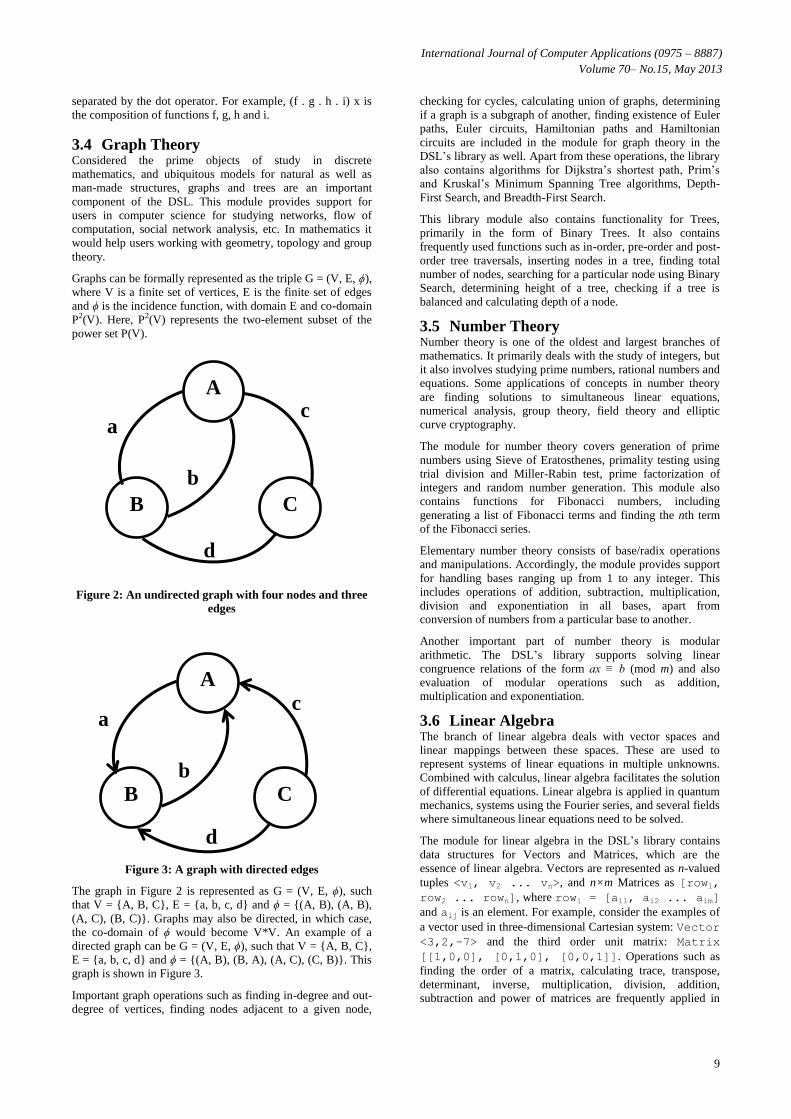
3.4 Graph Theory Considered the prime objects of study in discrete

mathematics, and ubiquitous models for natural as well as

man-made structures, graphs and trees are an important

component of the DSL. This module provides support for

users in computer science for studying networks, flow of

computation, social network analysis, etc. In mathematics it

would help users working with geometry, topology and group

theory.

Graphs can be formally represented as the triple G = (V, E, ϕ),

where V is a finite set of vertices, E is the finite set of edges

and ϕ is the incidence function, with domain E and co-domain

P2(V). Here, P2(V) represents the two-element subset of the

power set P(V).

Figure 2: An undirected graph with four nodes and three

edges

Figure 3: A graph with directed edges

The graph in Figure 2 is represented as G = (V, E, ϕ), such

that V = {A, B, C}, E = {a, b, c, d} and ϕ = {(A, B), (A, B),

(A, C), (B, C)}. Graphs may also be directed, in which case,

the co-domain of ϕ would become V*V. An example of a

directed graph can be G = (V, E, ϕ), such that V = {A, B, C},

E = {a, b, c, d} and ϕ = {(A, B), (B, A), (A, C), (C, B)}. This

graph is shown in Figure 3.

Important graph operations such as finding in-degree and out-

degree of vertices, finding nodes adjacent to a given node,

checking for cycles, calculating union of graphs, determining

if a graph is a subgraph of another, finding existence of Euler

paths, Euler circuits, Hamiltonian paths and Hamiltonian

circuits are included in the module for graph theory in the

DSL’s library as well. Apart from these operations, the library

also contains algorithms for Dijkstra’s shortest path, Prim’s

and Kruskal’s Minimum Spanning Tree algorithms, Depth-

First Search, and Breadth-First Search.

This library module also contains functionality for Trees,

primarily in the form of Binary Trees. It also contains

frequently used functions such as in-order, pre-order and post-

order tree traversals, inserting nodes in a tree, finding total

number of nodes, searching for a particular node using Binary

Search, determining height of a tree, checking if a tree is

balanced and calculating depth of a node.

3.5 Number Theory Number theory is one of the oldest and largest branches of

mathematics. It primarily deals with the study of integers, but

it also involves studying prime numbers, rational numbers and

equations. Some applications of concepts in number theory

are finding solutions to simultaneous linear equations,

numerical analysis, group theory, field theory and elliptic

curve cryptography.

The module for number theory covers generation of prime

numbers using Sieve of Eratosthenes, primality testing using

trial division and Miller-Rabin test, prime factorization of

integers and random number generation. This module also

contains functions for Fibonacci numbers, including

generating a list of Fibonacci terms and finding the nth term

of the Fibonacci series.

Elementary number theory consists of base/radix operations

and manipulations. Accordingly, the module provides support

for handling bases ranging up from 1 to any integer. This

includes operations of addition, subtraction, multiplication,

division and exponentiation in all bases, apart from

conversion of numbers from a particular base to another.

Another important part of number theory is modular

arithmetic. The DSL’s library supports solving linear

congruence relations of the form ax ≡ b (mod m) and also

evaluation of modular operations such as addition,

multiplication and exponentiation.

3.6 Linear Algebra The branch of linear algebra deals with vector spaces and

linear mappings between these spaces. These are used to

represent systems of linear equations in multiple unknowns.

Combined with calculus, linear algebra facilitates the solution

of differential equations. Linear algebra is applied in quantum

mechanics, systems using the Fourier series, and several fields

where simultaneous linear equations need to be solved.

The module for linear algebra in the DSL’s library contains

data structures for Vectors and Matrices, which are the

essence of linear algebra. Vectors are represented as n-valued

tuples <v1, v2 ... vn>, and n×m Matrices as [row1,

row2 ... rown], where rowi = [ai1, ai2 ... aim]

and aij is an element. For example, consider the examples of

a vector used in three-dimensional Cartesian system: Vector

<3,2,-7> and the third order unit matrix: Matrix

[[1,0,0], [0,1,0], [0,0,1]]. Operations such as

finding the order of a matrix, calculating trace, transpose,

determinant, inverse, multiplication, division, addition,

subtraction and power of matrices are frequently applied in

A

C B

A

C B



10

matrix theory, and functions for the same have been included

in the library module.

The module also contains functions for checking properties of

a matrix or whether a matrix is of a certain type. Some of

these include checking if a matrix is symmetric, skew-

symmetric, orthogonal, involutory, 0/1, unit/identity matrix, a

zero matrix or a one matrix. In addition, a mapping function

for matrices allows the application of a single function to all

the elements of a matrix. The module contains functions for

generating unit matrices of order n, m×n zero and one

matrices.

For vectors, functions are developed for addition, subtraction,

multiplication (scalar/dot/inner product, vector product, scalar

triple product and vector triple product), calculating

magnitude of a vector, calculating angle between two vectors,

mapping a function to a vector, checking if a vector is a unit

vector, determining order of vectors and extracting an element

or even a range of elements from a vector. The module also

contains functions to find sum and difference of a list of

Vectors.

3.7 Combinatorics This branch of mathematics deals with the study of countable

discrete structures. This involves counting the structures,

determining criteria, and constructing and analyzing objects

satisfying these criteria. In computer science, combinatorics is

used frequently in analysis of algorithms to obtain estimates

and formulas.

For users involved in computational combinatorics, this DSL

would be helpful as it has a module consisting of frequently

used functions such as those to find factorials, permutations

and combinations, generate permutation and combination lists

and also to generate random permutations using the Fisher-

Yates/Knuth shuffle algorithm.

4. IMPLEMENTATION AND RESULTS This section describes modules from the DSL’s library,

including declaration of these modules and a few sample

functions with results for every module. In addition, this

section also contains results of applications developed using

the DSL.

4.1 Mathematical Logic The module for mathematical logic contains the following

declaration for exporting functions to users’ programs:

module MPL.Logic.Logic

(

and',

or',

xor,

xnor,

nand,

nor,

equals,

implies,

(/\),

(\/),

(==>),

(<=>),

notL,

andL,

orL,

xorL,

xnorL,

nandL,

norL

)

where

Here, MPL.Logic.Logic is the module’s name, indicating

that the file is stored in the directory MPL/Logic and is

named Logic.hs. This declaration is followed by

definitions for each of the functions mentioned.

For example, consider the definition of the function for logical

implication:

implies :: Bool -> Bool -> Bool

implies a b

| (a == True)&&(b == False) = False

| otherwise = True

In accordance with the objective of creating a notation close

to the one actually used in discrete mathematics, an operator

for logical implication is defined as follows:

(==>) :: Bool -> Bool -> Bool

a ==> b = implies a b

This provides syntactic sugar and improves readability. Now,

the function for logical implication may be called by the user

in any of the following three ways, all giving the same result -

False:

implies True False

True `implies` False

True ==> False

As mentioned in 3.1, this module also defines functions which

work on a list of Boolean values. The difference between the

names of these functions and those of unary or binary

functions is that they contain an additional ‘L’ as suffix,

indicating that they operate on lists. A common operation is to

find the XOR (Exclusive OR) of a list of values. Since the

module already contains a function for finding the XOR of

two values, it can be used to XOR the result of XOR of two

values with the next value. Repeating this process for the

length of the list gives a single final Boolean value. Such

functions for lists of Boolean values are implemented using

Haskell’s foldl1 function. The xorL function is defined as:

xorL :: [Bool] -> Bool

xorL a = foldl1 (xor) a

Here, a represents a list of Bool. An example of this

function’s usage is:

xorL [True, False, True, True, False]

This returns the Bool value True. The results of invoked

functions and sample usage of operators are shown in Figure

12.

4.2 Set Theory Under set theory, the library contains modules for working on

Sets and Relations.

4.2.1 Sets The module for Sets is declared as:

module MPL.SetTheory.Set



11

(

Set(..),

set2list,

union, unionL,

intersection,

intersectionL,

difference,

isMemberOf,

cardinality,

isNullSet,

isSubset,

isSuperset,

powerSet,

cartProduct,

disjoint,

disjointL,

sMap

)

where

The function union is defined as:

union :: Ord a => Set a -> Set a -> Set a

union (Set set1) (Set set2)

= Set $ (sort . nub) (set1 ++ [e |

e <- set2, not (elem e set1)])

This is based on the definition that the union of two sets is the

set containing all elements from that first set, and all elements

from the second set that are not in the first. In addition,

duplicates from this set are removed and this resultant set is

sorted. If this function is called as union (Set

{2,4,6}) (Set {1,2,3}), the output would be Set

{1,2,3,4,6}.

A common set operation is that of finding the Cartesian

product of two sets. In the library module, it is defined as:

cartProduct :: Ord a => Set a -> Set a ->

[(a,a)]

cartProduct (Set set1) (Set set2)

= Set [(x,y) | x <- set1', y <- set2']

where

set1' = (sort . nub) set1

set2' = (sort . nub) set2

This function may be called as cartProduct (Set

{1,2}) (Set {3,4}) to produce the result Set

{(1,3),(1,4),(2,3),(2,4)}.

In several conditions, it is requires to check if two sets are

disjoint. For this, the module contains the function

disjoint, and it is defined as:

disjoint :: Ord a => Set a -> Set a ->

Bool

disjoint (Set s1) (Set s2) = isNullSet $

intersection (Set s1) (Set s2)

If a user were to invoke this function as disjoint (Set

{1,3..10}) (Set {2,4..10}), then he/she would get

back True as the output. These results are shown in Figure

14.

4.2.2 Relations The module for Relations is declared as:

module MPL.SetTheory.Relation

(

Relation(..),

relation2list,

getFirst,

getSecond,

elemSet,

returnFirstElems,

returnSecondElems,

isReflexive,

isIrreflexive,

isSymmetric,

isAsymmetric,

isAntiSymmetric,

isTransitive,

rUnion,

rUnionL,

rIntersection,

rIntersectionL,

rDifference,

rComposite,

rPower,

reflClosure,

symmClosure,

tranClosure,

isEquivalent,

isWeakPartialOrder,

isWeakTotalOrder,

isStrictPartialOrder,

isStrictTotalOrder

)

where

Consider the definition for the isTransitive function:

isTransitive :: Eq a => Relation a ->

Bool

isTransitive (Relation r)

= andL [(a,c) èlem` r | a <- elemSet r,

b <- elemSet r, c <- elemSet r, (a,b)

èlem` r, (b,c) èlem` r]

This function may be called by the user as isTransitive

(Relation {(1,1),(1,2),(2,1)}), which would

return False. However, the call isTransitive

(Relation {(1,1),(1,2),(2,1),(2,2)}) would

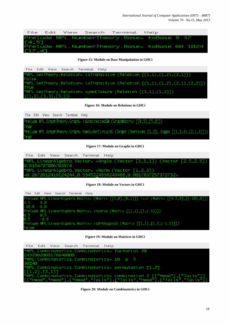
return True. This result is shown in Figure 16.

The symmClosure function returns symmetric closure of

the relation passed to it. It is defined as:

symmClosure :: Ord a => Relation a ->

Relation a

symmClosure (Relation r) = rUnion

(Relation r) (rPower (Relation r) (-1))

This function uses the property that symmetric closure of a

relation is the union of that relation with its inverse. Calling

the function as symmClosure (Relation

{(1,1),(1,3)}) would give the result as Relation

{(1,1),(1,3),(3,1)}.

4.3 Graph Theory Under graph theory, the library contains modules for Graphs

and Trees.



12

4.3.1 Graphs Declaration for the module on graphs is:

module MPL.GraphTheory.Graph

(

Vertices(..),

vertices2list,

Edges(..),

edges2list,

Graph(..),

GraphMatrix(..),

graph2matrix,

getVerticesG,

getVerticesGM,

numVerticesG,

numVerticesGM,

getEdgesG,

getEdgesGM,

numEdgesG,

numEdgesGM,

convertGM2G,

convertG2GM,

gTransposeG,

gTransposeGM,

isUndirectedG,

isUndirectedGM,

isDirectedG,

isDirectedGM,

unionG,

unionGM,

addVerticesG,

addVerticesGM,

verticesInEdges,

addEdgesG,

addEdgesGM,

areConnectedGM,

numPathsBetweenGM,

adjacentNodesG,

adjacentNodesGM,

inDegreeG,

inDegreeGM,

outDegreeG,

outDegreeGM,

degreeG,

degreeGM,

hasEulerCircuitG,

hasEulerCircuitGM,

hasEulerPathG,

hasEulerPathGM,

hasHamiltonianCircuitG,

hasHamiltonianCircuitGM,

countOddDegreeV,

countEvenDegreeV,

hasEulerPathNotCircuitG,

hasEulerPathNotCircuitGM,

isSubgraphG,

isSubgraphGM

)

where

As stated in section 3.4, the module contains functions which

work on graphs defined both formally and as matrices.

Functions for the former have ‘G’ as suffix, while functions

for the latter have ‘GM’ as suffix. The implementation of

functions for both is made possible by the functions

convertG2GM and convertGM2G, which convert between

the formal and matrix representations.

Consider the function for determining if a graph is undirected:

isUndirectedGM :: Ord a => GraphMatrix a

-> Bool

isUndirectedGM (GraphMatrix gm)

= (GraphMatrix gm) == gTransposeGM

(GraphMatrix gm)

When called as isUndirectedGM (GraphMatrix

[[0,5],[5,0]]), True is returned. The invocation of

functions for graphs is shown in Figure 17.

Using the property of that a graph has an Euler circuit only if

all vertices have even degree, the function

hasEulerCircuitG is defined as:

hasEulerCircuitG :: Ord a => Graph a ->

Bool

hasEulerCircuitG (Graph g)

= and [ even $ (degreeG (Graph g)

(Vertices [v])) | v <- vertices2list $

getVerticesG (Graph g)]

Thus, an invocation such as hasEulerCircuitG

(Graph (Vertices {1,2}, Edges

{(1,2,4),(2,1,3)})) would result in a return of True.

4.3.2 Trees The module for trees has the following declaration:

module MPL.GraphTheory.Tree

(

BinTree(..),

inorder,

preorder,

postorder,

singleton,

treeInsert,

treeSearch,

reflect,

height,

depth,

size,

isBalanced

)

where

The functions inorder, preorder and postorder are

functions for tree traversal. The definition for preorder is:

preorder :: BinTree a -> [a]

preorder Leaf = []

preorder (Node x t1 t2) = [x] ++ preorder

t1 ++ preorder t2

If we consider the following BinTree:

tree =

Node 4

(Node 2

(Node 1 Leaf Leaf)

(Node 3 Leaf Leaf))

(Node 7

(Node 5

Leaf

(Node 6 Leaf Leaf))

(Node 8 Leaf Leaf))



13

Then the function call, preorder tree, would generate

the result [4,2,1,3,7,5,6,8].

In essence, the BinTree data type is a Binary Search Tree.

The function treeSearch, is an implementation of the

Binary Search algorithm and has the following definition:

treeElem :: Ord a => a -> BinTree a ->

Bool

treeElem x Leaf = False

treeElem x ( Node a left right )

| x == a = True

| x < a = treeElem x left

| x > a = treeElem x right

The function isBalanced recursively checks if the height

of all nodes at the same level are equal. The definition of this

function makes use of the height function and is as follows:

isBalanced :: BinTree a -> Bool

isBalanced Leaf = True

isBalanced (Node x t1 t2) = isBalanced t1

&& isBalanced t2 && (height t1 == height

t2)

If this function is applied on tree as isBalanced tree,

the output would be False. The results of functions for

Trees are shown in Figure 13.

4.4 Number Theory Under number theory, the library contains the following

modules:

4.4.1 Base/Radix Manipulation This module has the description:

module MPL.NumberTheory.Base

(

toBase,

fromBase,

toAlphaDigits,

fromAlphaDigits

)

where

The function toBase converts a decimal number into the

equivalent form of a specified base/radix. It has the definition:

toBase :: Int -> Int -> [Int]

toBase base v = toBase' [] v where

toBase' a 0 = a

toBase' a v = toBase' (r:a) q where

(q,r) = v `divMod` base

When invoked as toBase 8 37 or as 37 `toBase` 8,

the result would be [4,5], which is read as 45, octal for 37.

The result of toBase is also shown in Figure 15.

4.4.2 Fibonacci Series The module on Fibonacci series contains two functions, fib

and fibSeries. The function fib takes an integer as

parameter and returns the term at that index in the Fibonacci

series. It is defined as:

fib n = round $ phi ** fromIntegral n /

sq5

where

sq5 = sqrt 5 :: Double

phi = (1 + sq5) / 2

If called as fib 10, the output is 55.

The fibSeries function takes an integer as parameter and

returns the Fibonacci series as a list of integers. The definition

is:

fibSeries n = [fib i | i <- [1..n]]

If a user wants to obtain the first 10 numbers in the Fibonacci

series, he/she has to call the function as fibSeries 10,

which gives the result [1,1,2,3,5,8,13,21,34,55].

4.4.3 Modular Arithmetic This module has the description:

module MPL.NumberTheory.Modular

(

modAdd,

modSub,

modMult,

modExp,

isCongruent,

findCongruentPair,

findCongruentPair1

)

where

The modExp function is the function for modular

exponentiation. It takes the numbers a, b and m as parameters

and computes the value of ab mod m. The definition is:

modExp a b m = modexp' 1 a b

where

modexp' p _ 0 = p

modexp' p x b =

if even b

then modexp' p (mod (x*x) m)

(div b 2)

else modexp' (mod (p*x) m) x

(pred b)

If invoked as modExp 112 34 546, the integer 532 is

returned.

4.4.4 Prime Numbers This module has the following description:

module MPL.NumberTheory.Primes

(

primesTo,

primesBetween,

firstNPrimes,

isPrime,

nextPrime,

primeFactors

)

where

The function primesTo generates all prime numbers less

than or equal to the number passed as parameter, using the

Sieve of Eratosthenes. Its definition is:

primesTo :: Integer -> [Integer]



14

primesTo 0 = []

primesTo 1 = []

primesTo 2 = [2]

primesTo m = 2 : sieve [3,5..m]

The invocation primesTo 20 gives the output:

[2,3,5,7,11,13,17,19].

4.5 Linear Algebra Under linear algebra, the library has modules for Vectors and

Matrices.

4.5.1 Vectors This module’s description is:

module MPL.LinearAlgebra.Vector

(

Vector(..),

vDim,

vMag,

vec2list,

vAdd,

vAddL,

(<+>),

vSub,

vSubL,

(<->),

innerProd,

(<.>),

vAngle,

scalarMult,

(<*>),

isNullVector,

crossProd,

(><),

scalarTripleProd,

vectorTripleProd,

extract,

extractRange,

areOrthogonal,

vMap,

vNorm

)

where

The vAngle function returns the angle between two Vectors.

It has the definition:

vAngle :: Floating a => Vector a ->

Vector a -> a

vAngle (Vector []) (Vector []) = 0

vAngle (Vector v1) (Vector v2) = acos (

(innerProd (Vector v1) (Vector v2)) / (

(vMag (Vector v1)) * (vMag (Vector v2)))

As shown in Figure 18, when invoked as vAngle (Vector

[1,1,1]) (Vector [2.5,2.5]), the result is

0.6154797086703874.

The function scalarTripleProduct is based on the

functions innerProduct and crossProduct. It is

defined as:

scalarTripleProd a b c = innerProd a

(crossProd b c)

To normalize a Vector, the vNorm function can be used. It

has the definition:

vNorm (Vector v) = scalarMult (1/(vMag

(Vector v))) (Vector v)

If called as vNorm (Vector [1,2,3]), the output is the

Vector: <0.2672612419124244,0.5345224838248488,0.

8017837257372732>

4.5.2 Matrices The module for matrices has the following description:

module MPL.LinearAlgebra.Matrix

(

Matrix(..),

mAdd,

mAddL,

(|+|),

mSub,

(|-|),

mTranspose,

mScalarMult,

(|*|),

mMult,

mMultL,

(|><|),

numRows,

numCols,

mat2list,

determinant,

inverse,

mDiv,

(|/|),

extractRow,

extractCol,

extractRowRange,

extractColRange,

mPower,

trace,

isInvertible,

isSymmetric,

isSkewSymmetric,

isRow,

isColumn,

isSquare,

isOrthogonal,

isInvolutory,

isZeroOne,

isZero,

isOne,

isUnit,

zero,

zero’,

one,

one’,

unit,

mMap

)

where

The mMult function performs multiplication of two matrices

and returns the resultant matrix. Its definition is:

mMult :: Num a => Matrix a -> Matrix a ->

Matrix a



15

mMult (Matrix m1) (Matrix m2) = Matrix $

[ map (multRow r) m2t | r <- m1 ]

where

(Matrix m2t) = mTranspose (Matrix

m2)

multRow r1 r2 = sum $ zipWith (*)

r1 r2

To add syntactic sugar, the module exports the operator |><|

for multiplying two matrices. Thus, if a user wishes to

multiply a Matrix m1, which is Matrix [[1,0],[0,1]]

and a Matrix m2, which is Matrix [[4.5,8],[(-

10),6]], he/she can call either mMult m1 m2 or m1

|><| m2, to get the output as Matrix

[[4.5,8.0],[(-10.0),6.0]]. The usage and result is

shown in Figure 19.

Another common operation is to find inverse of a matrix. In

this module, the function inverse is defined using the

functions cofactorM and determinant as:

inverse (Matrix m) = Matrix $ map (map (*

recip det)) $ mat2list $ cofactorM

(Matrix m)

where

det = determinant (Matrix m)

If called as inverse (Matrix [[1,1],[1,(-1)]]),

the result is the matrix: Matrix [[0.5,0.5],[0.5,(-

0.5)]].

The module contains several functions to check for properties

of a matrix. One of these is isOrthogonal, which is to

check if a matrix is orthogonal. Using the functions

mTranspose and inverse it is easily defined as:

isOrthogonal (Matrix m) = (mTranspose

(Matrix m) == inverse (Matrix m))

When it is used as isOrthogonal (Matrix

[[1,1],[1.2,(-1.5)]]), the output is False.

4.6 Combinatorics This module has the description:

module MPL.Combinatorics.Combinatorics

(

factorial,

c,

p,

permutation,

shuffle,

combination

)

where

The function definition for factorial is:

factorial :: Integer -> Integer

factorial n

| (n == 0) = 1

| (n > 0) = product [1..n]

| (n < 0) = error "Usage -

factorial n, where 'n' is non-negative."

This function can return arbitrarily large integers since its

return type is Integer. When factorial 5 is called,

120 is returned as the result.

The factorial function acts as a base for other functions

in the module. For example, the function p returns the number

of possible permutations of r objects from a set of n given by

nPr. It is defined as:

p :: Integer -> Integer -> Integer

p n r = div (factorial a) (factorial (a-

b))

where

a = max n r

b = min n r

When this function is called as p 10 5 or 10 `p` 5,

30240 is the output. Usage of these functions is shown in

Figure 20.

4.7 Applications This subsection contains sample results from applications

developed using the DSL.

4.7.1 Ciphers Fig. 4 and Fig. 5 show the output of a program developed in

the DSL for enciphering and deciphering of messages using

Caesar cipher and Transposition cipher.

4.7.2 RSA Encryption and Decryption Sample execution results of a program for implementing RSA

encryption system using the DSL are shown in Fig. 6 and Fig.

7. This program was developed using the library modules on

modular arithmetic, MPL.NumberTheory.Modular, and

on prime numbers, MPL.NumberTheory.Primes.

Figure 4: Enciphering using Caesar cipher



16

4.7.3 Diffie-Hellman Key Exchange A sample output of a program developed using the DSL for

Diffie-Hellman Key Exchange protocol is shown in Fig. 8.

The two users must have a common primitive root and a

prime number. The shared key and public keys are calculated

using the users’ private keys.

4.7.4 Simultaneous Linear Equations Since the DSL’s library provides support for Matrices, it is

easy to develop a program for solving simultaneous linear

equations. Fig. 9 shows an output for solving the two

equations in two variables: x + 2y = 4 and x + y = 1. It is also

possible to solve linear equations in n variables using n or

more equations.

4.7.5 Mersenne Prime Numbers The DSL’s module on prime numbers under number theory

allows for efficient determination of Mersenne prime

numbers. Mersenne prime numbers are prime numbers of the

form 2q - 1, where q is also a prime number. Fig. 10 shows the

output as a list of powers q, between 2 and 1000, which result

in Mersenne primes. Fig. 11 shows the output as a list all

Mersenne prime numbers less than 2100.

Figure 5: Deciphering using Transposition cipher

Figure 6: Encryption using RSA

Figure 7: Decryption using RSA

Figure 8: Generating Shared Key using Diffie-Hellman

Key Exchange protocol

Figure 9: Solving simultaneous linear equations



17

5. SCREENSHOTS OF IMPLEMENTED

LIBRARY MODULES

Figure 10: Powers of Mersenne prime numbers

Figure 11: Mersenne prime numbers having powers from 2 to 100

Figure 12: Module on Mathematical Logic in GHCi

Figure 13: Module on Trees in GHCi

Figure 14: Module on Sets in GHCi



18

Figure 15: Module on Base Manipulation in GHCi

Figure 16: Module on Relations in GHCi

Figure 17: Module on Graphs in GHCi

Figure 18: Module on Vectors in GHCi

Figure 19: Module on Matrices in GHCi

Figure 20: Module on Combinatorics in GHCi



19

6. FUTURE SCOPE Since discrete mathematics is a vast area of study, it is not

possible to include all topics in the library during the initial

stages of development. In the future, modules for group

theory, information theory, geometry, topology and

theoretical computer science can be added. Additionally, the

preprocessor can be constantly updated to handle new

modules and new features in existing ones. Apart from this,

based on feedback and suggestions from users, the syntax of

this DSL can be improved to suit their needs.

7. CONCLUSION Discrete mathematics plays a central role in the fields of

modern cryptography, social networking, digital signal and

image processing, computational physics, analysis of

algorithms, languages and grammars. The language

developed, owing to its syntax, helps computer scientists and

mathematicians to work in an easier and more efficient

manner as compared to that while using a General Purpose

Language (GPL). This language would also be helpful to

those learning and teaching discrete mathematics.

8. REFERENCES [1] Fowler, M. 2010, “Domain-Specific Languages”,

Addison-Wesley Professional.

[2] Taha, W. 2008, “Domain Specific Languages”, IEEE

International Conference on Computer Engineering and

Systems (ICESS).

[3] Mernik, M., Heering, J., and Sloane, A. M. 2005, “When

and How to Develop Domain-Specific Languages”,

ACM Computing Surveys (CSUR).

[4] Ghosh, D. 2011, “DSLs in Action”, Manning

Publications Co.

[5] Karsai, G., Krahn, H., Pinkernell, C., Rumpe, B.,

Schindler, M., and Volkel, S. 2009, “Design Guidelines

for Domain Specific Languages”, Proceedings of DSM

2009.

[6] Hughes, J., "Why Functional Programming Matters",

The Computer Journal, 1989.

[7] Goldberg, B., “Functional Programming Languages”,

ACM Computing Surveys, Vol. 28, No. 1, March 1996.

[8] Hudak, P. 1996. "Building domain-specific embedded

languages", ACM Computing Surveys, December 1996.

[9] http://www.haskell.org/haskellwiki/Introduction.

Introduction to Haskell, retrieved on October 22, 2012.

[10] http://www.haskell.org/ghc/docs/7.0.4/html/users_guide/i

ndex.html. The Glorious Glasgow Haskell Compilation

System User’s Guide, Version 7.0.4

A Domain-Specific Language for Discrete Mathematics · discrete mathematics by implementing it as a...

Documents

Transcript of A Domain-Specific Language for Discrete Mathematics · discrete mathematics by implementing it as a...