JJPC: 2641

Journal of Process Control xxx (xxxx) xxx

Contents lists available at ScienceDirect

Journal of Process Control

journal homepage: www.elsevier.com/locate/jprocont

A distributed feedback-based online process optimization frameworkfor optimal resource sharingI

Dinesh KrishnamoorthyDepartment of Chemical Engineering, Norwegian University of Science and Technology (NTNU), Trondheim, Norway

a r t i c l e i n f o

Article history:

Received 17 June 2020Received in revised form12 September 2020Accepted 22 November 2020Available online xxxx

Keywords:

Distributed RTOFeedback-based RTOIndustrial symbiosis

a b s t r a c t

Distributed real-time optimization (RTO) enables optimal operation of large-scale process systems withcommon resources shared across several clusters. Typically in distributed RTO, the different subsystemsare optimized locally, and a centralized master problem is used to coordinate the different subsystemsin order to reach system-wide optimal operation. This is especially beneficial in industrial symbiosis,where only limited information can be shared between the different clusters. However, one of the mainchallenges with this approach is the need to solve numerical optimization problems online for eachsubsystem. With the recent surge of interest in feedback optimizing control, where the optimizationproblem is converted into a feedback control problem, this paper proposes a distributed feedback-based RTO (DFRTO) framework for optimal resource sharing in an industrial symbiotic setting. In thisapproach, a master coordinator updates the shadow price for the shared resource, and the differentsubsystems locally optimize their operation using feedback control for the given shadow price. Theproposed framework is shown to converge to a stationary point of the system-wide optimizationproblem, and is demonstrated using an industrial symbiotic offshore oil and gas production systemwith shared resources.

© 2020 The Author(s). Published by Elsevier Ltd. This is an open access article under the CC BY license(http://creativecommons.org/licenses/by/4.0/).

1. Introduction1

In the face of growing competition, stringent emission reg-2ulations, and increased necessity for sustainable manufacturing,3there is a clear need to focus on energy and resource efficiency4in order to reduce waste. In the process and manufacturing in-5dustries, there is an increasing trend of industrial symbiosis, where6different organizations come together in an industrial cluster/eco-7park, and share resources and equipment in a mutually beneficial8manner.9

As the process industry is embracing industrial symbiosis, this10creates new challenges. Finding a feasible and optimal operation11for a large-scale system is challenging and typically requires12information about the entire process, in the form of models, real13time measurements, local constraints and the economic objective.14This challenge is only amplified in an industrial symbiotic setting15with shared resources, since the different companies might be16reluctant to share information across the different organizations,17for example due to intellectual property rights, trade secrets, and18market competitiveness.19

I The author gratefully acknowledges financial support from the ResearchCouncil of Norway through the IKTPLUSS program (Project number 299585) andSFI SUBPRO.

E-mail address: dinesh.krishnamoorthy@ntnu.no.

One potential solution that facilitates industrial symbiosis is 20the distributed optimization framework, where the different sub- 21systems are locally modeled and optimized and a centralized 22master problem coordinates the subproblems. This addresses pri- 23vacy and data sharing issues, since only limited information is 24shared between the different subsystems [1]. There are different 25strategies that can be used to decompose a large-scale problem 26into several smaller subproblems. This can be broadly categorized 27into primal decomposition and dual decomposition [2]. 28

In primal decomposition, the different subproblems report 29the price they are willing to pay for the shared resource, and 30the master coordinator directly allocates the shared resource 31accordingly. However, this approach may require the subsystems 32to share additional knowledge about the local constraints to the 33master coordinator in order to ensure that the allocated resource 34is feasible for the subproblems. Therefore, this approach may not 35be suitable for industrial symbiosis [1]. 36

Dual decomposition, also known as Lagrangian decomposition, 37on the other hand is a price-based coordination, where the master 38coordinator sets the price of the shared resource, which regulates 39the local decision making in each subsystem. Unlike primal de- 40composition, this approach does not require information about 41the local constraints to be shared with the master coordinator, 42which makes it a favorable approach for industrial symbiosis. 43Both the primal and dual decomposition strategies involve it- 44eratively solving the subproblems and the master coordinator, 45

https://doi.org/10.1016/j.jprocont.2020.11.0060959-1524/© 2020 The Author(s). Published by Elsevier Ltd. This is an open access article under the CC BY license (http://creativecommons.org/licenses/by/4.0/).

JJPC: 2641

D. Krishnamoorthy Journal of Process Control xxx (xxxx) xxx

where each subproblem solves a numerical optimization problem1at each iteration.2

Decomposition strategies are a popular area of research, in the3context of both model predictive control (MPC) as well as real-4time optimization (RTO). In this paper, we focus on steady-state5real time optimization, and the reader is simply referred to [3]6for a comprehensive compilation of literature on distributed MPC.7Research on distributed RTO for large-scale process systems has8been gaining increasing interest, with some notable works such9as [1,4–8] to name a few. However, the use of distributed RTO10methods in practice remains rather low, if not nonexistent [1].11The main reasons for this is attributed to the computational cost12of solving the numerical optimization problems online and the13slow convergence rate.14

Currently, there is active research to improve the rate of15convergence, such that the master and subproblems converge16to a feasible optimal solution in a small number of iterations/17communication rounds. Some notable works in this direction18include fast ADMM [9], Newton-based methods (ALADIN) [10],19and quadratic approximations [1] to name a few.20

Despite the algorithmic developments to improve the con-21vergence rate, the subproblems still need to solve numerical22optimization problems online at each iteration, which is a more23fundamental limiting factor for practical implementation of real24time optimization due to computational and numerical robust-25ness issues [11,12]. In addition to the computational cost of26solving numerical optimization problems online, the lack of tech-27nical expertise and competence to implement and maintain such28numerical optimization-based RTO is one of the major imped-29ing factors for practical application in many industries. The ex-30pected benefits of optimization are at risk without regular main-31tenance and monitoring [13], which requires expert knowledge.32As pointed out by the authors in [14], the performance degra-33dation due to lack of maintenance and support often leads to34the application being turned off by the operator. For this reason,35many traditional process industries still prefer to optimize their36operations using simple feedback control tools [15]. Therefore,37there is a need to develop a distributed framework with limited38information exchange that eliminates the need to solve numerical39optimization problems online. This would enable industrial sym-40biosis even in the case where some participating organizations41prefer to use only feedback control.42

Recently, there has been a surge of interest in achieving op-43timal operation using feedback control. This is often referred to44as “feedback optimizing control” [16,17] or “direct input adapta-45tion” [18], where the aim is to translate the economic objectives46into control objectives, thereby achieving optimal process opera-47tion by directly manipulating the input using feedback control.48The concept of feedback optimizing control dates back to the491980s [16] motivated by the industrial and academic gap. Some50recent survey articles such as [18–22] provides a good overview51of the different feedback-based RTO methods that have been52developed across several research groups since then. In addition53to process control, feedback-based optimization is also gaining54popularity in other application domains such as power systems,55see for example [23,24].56

Feedback optimizing control, in general, is more suited for unit57operations, or for small-scale processes. In large-scale systems, it58becomes easier to design feedback optimizing control for small59subgroups of processes. This leads to a decentralized control60structure, where some clusters of operating units are optimized61locally without any coordination. However, when the system is62coupled in one form or the other, system-wide optimal operation63does not result from the aggregates of individual operating units64in a decentralized fashion. This was also discussed in detail in the65same paper that introduced the concept of feedback optimizing66

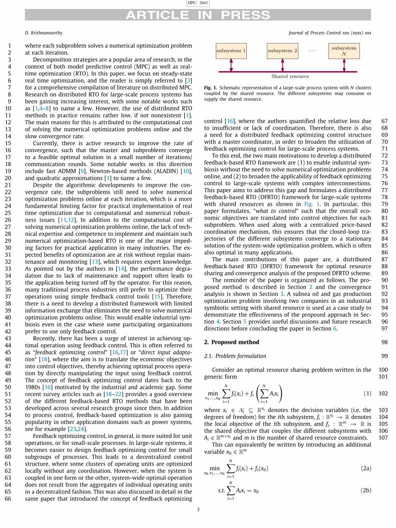
Fig. 1. Schematic representation of a large-scale process system with N clusterscoupled by the shared resource. The different subsystems may consume orsupply the shared resource.

control [16], where the authors quantified the relative loss due 67to insufficient or lack of coordination. Therefore, there is also 68a need for a distributed feedback optimizing control structure 69with a master coordinator, in order to broaden the utilization of 70feedback optimizing control for large-scale process systems. 71

To this end, the two main motivations to develop a distributed 72feedback-based RTO framework are (1) to enable industrial sym- 73biosis without the need to solve numerical optimization problems 74online, and (2) to broaden the applicability of feedback optimizing 75control to large-scale systems with complex interconnections. 76This paper aims to address this gap and formulates a distributed 77feedback-based RTO (DFRTO) framework for large-scale systems 78with shared resources as shown in Fig. 1. In particular, this 79paper formulates, “what to control” such that the overall eco- 80nomic objectives are translated into control objectives for each 81subproblem. When used along with a centralized price-based 82coordination mechanism, this ensures that the closed-loop tra- 83jectories of the different subsystems converge to a stationary 84solution of the system-wide optimization problem, which is often 85also optimal in many applications. 86

The main contributions of this paper are, a distributed 87feedback-based RTO (DFRTO) framework for optimal resource 88sharing and convergence analysis of the proposed DFRTO scheme. 89

The reminder of the paper is organized as follows. The pro- 90posed method is described in Section 2 and the convergence 91analysis is shown in Section 3. A subsea oil and gas production 92optimization problem involving two companies in an industrial 93symbiotic setting with shared resource is used as a case study to 94demonstrate the effectiveness of the proposed approach in Sec- 95tion 4. Section 5 provides useful discussions and future research 96directions before concluding the paper in Section 6. 97

2. Proposed method 98

2.1. Problem formulation 99

Consider an optimal resource sharing problem written in the 100generic form 101

minx1,...,xN

NX

i=1

fi(xi) + fs

NX

i=1

Aixi

!(1) 102

where xi 2 Xi ✓ Rni denotes the decision variables (i.e. the 103degrees of freedom) for the ith subsystem, fi : Rni ! R denotes 104the local objective of the ith subsystem, and fs : Rm ! R is 105the shared objective that couples the different subsystems with 106Ai 2 Rm⇥ni and m is the number of shared resource constraints. 107

This can equivalently be written by introducing an additionalvariable x0 2 Rm

minx0,x1,...,xN

NX

i=1

fi(xi) + fs(x0) (2a)

s.t.NX

i=1

Aixi = x0 (2b)

3

JJPC: 2641

D. Krishnamoorthy Journal of Process Control xxx (xxxx) xxx

which can be further condensed as

minx0,x1,...,xN

NX

i=0

fi(xi) (3a)

s.t.NX

i=0

Aixi = 0 (3b)

where f0 = fs and A0 = �Im.1

Remark 1. Note that the shared resource may either be con-2sumed or produced by the different subsystems. xi > 0 implies3that the shared resource is being consumed by subsystem i, and4xi < 0 implies that the shared resource is produced by subsystem5i.6

Assumption 1. fi(·) is smooth, but may be nonconvex, Xi is a7closed convex set, and Ai has full rank.8

The Lagrangian of (3) is given by,9

L(x0, . . . , xN , �) =NX

i=0

fi(xi) + �TNX

i=0

Aixi (4)10

where � 2 Rm is the Lagrange multiplier of the coupling con-11straint.12

Defining x := {x0, . . . , xN}, the necessary conditions of opti-mality for this problem can be stated as

rxL(x, �) =NX

i=0

rxif (xi) +

NX

i=0

ATi� = 0 (5a)

NX

i=0

Aixi = 0 (5b)

and a point (x⇤, �⇤) that satisfies (5) is known as a KKT point, or13a stationary point.14

For the KKT point to be a local optimum, we further require15that the Hessian of the Lagrangian H(x, �) is positive definite,16that is, dT

H(x, �)d > 0 holds for all d 6= 0 such that ATd = 0,17

where A := [A0, A1 . . . , An]T. If this is true, then strong second18order sufficient conditions (SSOSC) is said to hold at the KKT point19(x⇤, �⇤).20

The objective here is to drive the process to a KKT point of21(3) in a distributed fashion with limited information exchange22using only simple feedback controllers, such as PID control. To23do this, we first decouple the subproblems and then identify24self-optimizing controlled variables for each subsystem.25

Notice that the cost (3a) is additively separable, but the shared26resource constraint (3b) couples the different subproblems to-27gether. We see that the Lagrangian (4) is additively separable.28

29

Li(xi, �) = fi(xi) + �TAixi (6)30

We can therefore decompose the problem using the Lagrangian31decomposition framework by relaxing the coupling constraints32[25]. This is known as dual decomposition or Lagrangian decom-33position. In the standard distributed RTO framework, the different34subproblems solve the unconstrained optimization problem35

x⇤i(�) = arg min

xi2Xi

Li(xi, �) (7)36

for a given �, and the master coordinator updates �, typically37using the dual ascent step,38

�+ = � + ↵

NX

i=0

Aix⇤i

(8)39

where ↵ = diag(↵1, . . . ,↵m) with ↵ > 0 is the step-size. 40Traditionally, the subproblems (7) and the master problem (8) are 41iteratively solved until convergence. 42

The Lagrangian decomposition framework has an economic in- 43terpretation, where the Lagrange multiplier � is the shadow price 44of the shared resource. Here the goal of the master coordinator 45is to find an equilibrium price for the shared resource such that 46the supply matches the demand in the micro market. In other 47words, when the supply of the shared resource increases, the 48master coordinator decreases the price � in order to encourage 49consumption by the subproblems. Similarly, if the demand for the 50shared resource increases, the master coordinator increases the 51price � to find the equilibrium price. Such problems have been 52studied extensively in general equilibrium theory, economics, 53resource allocation, optimal exchange etc. [25,26], and have also 54been studied in the context of process systems engineering (PSE), 55see for example [1,4,5] and the references therein. 56

However, in this paper, we do not want to explicitly solve 57(7), instead we want to translate the unconstrained optimization 58problem (7) into a feedback control problem. In other words, 59the objective is to find a self-optimizing controlled variable for each 60subproblem as a function of the shadow price ci(�), which when kept 61at a constant setpoint c

sp

ileads to optimal operation of the local 62

subsystem, and when the master coordinator updates the shadow 63price, leads to system-wide optimal operation.1 64

Remark 2. Note that the dual ascent step (8) in the master 65coordinator can be seen as a simple integral controller that drives 66the coupling constraint

PN

i=0 Aixi to zero, that is the price � is 67updated if the supply does not match the demand. 68

The ideal self-optimizing variable is the steady-state cost 69gradient which must be driven to a constant setpoint of zero, 70thereby satisfying the necessary condition of optimality (5). NCO- 71tracking control [27], extremum seeking control [28,29], Feedback 72RTO [30], hill-climbing control [31] etc. are some of the feedback 73optimizing control approaches in the RTO literature that use the 74steady-state cost gradient as the self-optimizing variable. 75

Therefore, for each subproblem (7), the self-optimizing vari- 76able ci(�) 2 Rni can be expressed as 77

ci(�) := rxiLi(�) = rxi

f (xi) + ATi� (9) 78

which must be driven to a constant setpoint of csp

i= 0. Note 79

that the controlled variable is now a function of the shadow price 80�, which is updated by the master coordinator using (8), just 81as in the traditional distributed RTO scheme. Controlling ci(�) 82requires the online estimation of the local cost gradient rxi

f (xi), 83which can be done using any suitable model-based or model- 84free gradient estimation scheme, see for example [22] and the 85references therein. 86

If the objective function is nonconvex, then controlling (9) 87may lead to some convergence issues. In order to make the 88dual decomposition approach robust and yield convergence, it is 89common in the distributed optimization framework to use the 90augmented Lagrangian function instead. Similarly, we can also 91consider the augmented Lagrangian in the distributed feedback- 92based RTO framework to ensure the convergence properties even 93in the case where fi(xi) is nonconvex. 94

The augmented Lagrangian of (3) can be expressed as 95

L⇢(x, �) =NX

i=0

fi(xi) + �TNX

i=0

Aixi +⇢

2

�����

NX

i=0

Aixi

�����

2

(10) 96

1 Note that for the sake of exposition, this is stated assuming that thestationary point is also the optimum point here.

4

JJPC: 2641

D. Krishnamoorthy Journal of Process Control xxx (xxxx) xxx

Fig. 2. Schematic representation of the proposed Distributed feedback based RTO framework. Anything inside the information boundary (depicted using gray dashedlines) is contained within the subsystem. The residual r and the shadow price � are the only variables that are shared across the different subsystems.

where an additional regularization term is added to the La-1grangian (4). Clearly, any stationary point of the augmented La-2grangian (10) is also a stationary point of the Lagrangian (4). The3different subproblems can then be expressed as an unconstrained4optimization problem for a given �,5

x⇤i(�) = arg min

xi2Xi

L⇢,i(xi, �) (11)6

where7

L⇢,i(xi, �) = fi(xi) + �TAixi +

⇢

2

�����

NX

i=0

Aixi

�����

2

(12)8

In the traditional distributed RTO, this is solved using the al-9ternating directions method of multipliers (ADMM), where the10ith subproblem is solved by fixing xj for all j 6= i, similar to11one pass of a Gauss–Seidel method [25]. In this paper, instead of12solving this problem using ADMM, we convert it into a feedback13control problem by controlling the steady-state gradient of the14augmented Lagrangian rxi

L⇢,i(�) to a constant setpoint of zero.15In this case, the self-optimizing variable ci(�) 2 Rni for each16subsystem is expressed as,17

ci(�) := rxif (xi) + A

Ti� + ⇢AT

i

NX

i=0

Aixi

| {z }=r

(13)18

where r =: PN

i=0 Aixi is the residual that represents the total19surplus or shortage of the shared resource (i.e supply/demand).20The master coordinator updates the shadow price � using the21dual ascent step (8) with ↵ = ⇢. Note that since the residual r22is a real-time measurement, the feedback-based approach does23not need to be solved in an alternating directions fashion.24

Remark 3. Compared to the self-optimizing controlled variable in25(9), we now need r in addition. Note that we do not need to share26information regarding the individual contribution/consumption27by each subsystem, but we only need the overall residual r .28

For a convex problem, the controlled variables (9) and (13)29converges to the same stationary point, since at the optimum30r = 0 (thanks to the integral action in the master coordinator)31and (7) and (11) are equivalent. One of the main motivation for32using (13) instead of (9) is to ensure convergence properties if33the objective function is nonconvex, which will be shown later in34Section 3.35

Apart from the advantages of feedback optimizing control36noted in Section 1, it also has other advantages. For example,37

the DFRTO approach can be implemented at higher sampling 38rates than the traditional distributed RTO framework, since we 39do not need to solve numerical optimization problems online. In 40addition, the proposed DFRTO approach does not need to wait 41for the process to reach steady-state before re-optimizing, thus 42alleviating the steady-state wait-time issue associated with the 43traditional RTO framework [8,11,12]. 44

Remark 4. Another advantage of the proposed DFRTO scheme is 45that the sampling time of the local controllers for the different 46subsystems may be chosen independently. The sampling time of 47the master coordinator (denoted by t, t + 1, . . .) may either be 48the same as the local controllers, or slower. 49

Remark 5. In the case where xi 2 Xi becomes optimally active, 50then the feedback control problem for the subsystem simply 51becomes an active constraint control problem [17]. 52

2.2. Distributed feedback-based RTO (DFRTO) 53

We now formulate the distributed feedback-based RTO frame- 54work, which is schematically shown in Fig. 2. The three main 55components of the DFRTO framework are : 56

1. For each subsystem i = 0, . . . ,N , estimate rxifi using the 57

local real time measurements.2 582. For each subsystem i = 0, . . . ,N , control 59

ci(�[t]) = rxifi + A

Ti�[t] + ⇢AT

i

NX

i=0

Aixi

| {z }=r

60

for a given shadow price �[t] to a constant setpoint of 61csp

i= 0 using simple feedback controllers. 62

3. At every sample time of the master coordinator t+1, gather 63the residual r[t + 1] = P

N

i=0 Aixi[t + 1] and update the 64shadow price 65

�[t + 1] = �[t] + ⇢

NX

i=0

Aixi[t + 1] (14) 66

in the centralized master coordinator, and broadcast �[t + 671] to the subsystems. 68

2 Direct measurements of the local cost fi is required when using model-freegradient estimation methods [22].

5

JJPC: 2641

D. Krishnamoorthy Journal of Process Control xxx (xxxx) xxx

The shadow price �[t] and the residual r are the only informa-1tion that are shared among the different subsystems. This is also2clearly shown in Fig. 2, with the information boundary for each3subsystem shown in gray dashed lines, and only � and r crosses4the information boundary of each subsystem.5

The traditional distributed optimization framework typically6requires several iterations between the subproblems and the7master coordinator to converge to a KKT point. However, in8the proposed distributed feedback-based RTO, we do not iterate9between the master and subproblem, since xi[t] is a real time10measurement, and not the solution to a numerical optimization11problem. Therefore the “iteration” is done in real-time, and as12time t ! 1, xi[t] computed by the different controllers con-13verges to a KKT-point of the original problem. This can be seen14as the traditional distributed RTO with a single iteration between15the master and subproblems with warm-starting at every time16step.17

3. Convergence analysis18

In this section we analyze the convergence properties of the19proposed distributed feedback-based RTO scheme for an opti-20mization problem of the form (3), where fi(xi) is possibly non-21convex, but smooth. We show that by using the proposed self-22optimizing controlled variable with the penalty parameter ⇢ cho-23sen sufficiently large, the system converges to a feasible set of24stationary solutions. Here we use the augmented Lagrangian (10)25as the merit function and show that it monotonically decreases26over time using the proposed framework. To show convergence of27the proposed method, we follow a similar framework as in [32],28where the augmented Lagrangian was used as the merit function29to guide convergence of nonconvex ADMM problems.30

Assumption 2 (Perfect Control). In each subsystem, we have per-31fect control such that ci(�[t]) = c

sp

ifor all i at each sampling time32

of the master coordinator. Furthermore we assume that there is33no communication delay for the globally shared variables r and34�.35

Assumption 3 (Lipschitz Continuous Gradient). The shared cost36f0(·) is smooth nonconvex, and has a Lipschitz continuous gra-37dient with a positive constant L0 > 0, i.e.38

krf0(a) � rf0(b)k L0ka � bk39

Definition 1 (Strong Convexity). For a, b 2 Rn, any function h :40Rn ! R is said to be � -strongly convex if41

h(a) � h(b) rh(a)T(a � b) � �

2ka � bk242

Assumption 4. The penalty parameter ⇢ in the self-optimizing43variable (13) is chosen sufficiently large such that44

(i) The augmented Lagrangian (10) is � -strongly convex in the45sense of Definition 146

(ii) ⇢� > 2L2047(iii) ⇢ > L048

Lemma 1 (Successive Boundedness of the Shadow Price). Suppose49Assumptions 2 and 3 hold, then the following inequalities hold50

k�[t + 1] � �[t]k2 L20kx0[t + 1] � x0[t]k2 (15)51

Proof. Assuming perfect control, at time t + 1, the controlled52variables for i = 0 is given by53

rx0 f0(x0[t + 1]) + AT0�[t] + ⇢AT

0

NX

i=0

Aixi[t + 1] = 054

From the master update step (14) at time t + 1, we have withA0 = �Im

rx0 f0(x0[t + 1]) + AT0�[t + 1] = 0

rx0 f0(x0[t + 1]) � �[t + 1] = 0

) �[t + 1] = rx0 f0(x0[t + 1]) (16)

From Assumption 3, we have

k�[t + 1] � �[t]k = krx0 f0(x0[t + 1]) � rx0 f0(x0[t])k L0kx0[t + 1] � x0[t]k

from which (15) follows. ⇤ 55

The following lemma bounds the successive difference of the 56overall unconstrained cost (10). 57

Lemma 2 (Successive Boundedness of the Augmented Lagrangian).Given Assumptions 2, 3 and 4, the following holds for the distributed

feedback-based RTO

L⇢(x[t + 1], �[t + 1]) � L⇢(x[t], �[t])

✓L20

⇢� �

2

◆kx0[t + 1] � x0[t]k2 (17)

�NX

i=1

�

2kxi[t + 1] � xi[t]k2

Proof. We split the L.H.S. into two parts,

L⇢(x[t + 1], �[t + 1]) � L⇢(x[t], �[t])= L⇢(x[t + 1], �[t + 1]) � L⇢(x[t + 1], �[t])| {z }

=A

+ L⇢(x[t + 1], �[t]) � L⇢(x[t], �[t])| {z }

=B

We start by bounding A

A =NX

i=0

fi(xi[t + 1]) + �T[t + 1]NX

i=0

Aixi[t + 1]

+ ⇢

2

�����

NX

i=0

Aixi[t + 1]�����

2

�NX

i=0

fi(xi[t + 1]) � �T[t]NX

i=0

Aixi[t + 1]

� ⇢

2

�����

NX

i=0

Aixi[t + 1]�����

2

= (�[t + 1] � �[t])

NX

i=0

Aixi[t + 1]!

From the master update step (14), 58

A = 1⇢

k�[t + 1] � �[t]k2 59

Now we consider B. Using Assumption 4.i and the definition ofstrong convexity,

B = L⇢(x[t + 1], �[t]) � L⇢(x[t], �[t])

NX

i=0

rxiL⇢,i(xi[t + 1])(xi[t + 1] � xi[t])

�NX

i=0

�

2kxi[t + 1] � xi[t]k2

6

JJPC: 2641

D. Krishnamoorthy Journal of Process Control xxx (xxxx) xxx

�NX

i=0

�

2kxi[t + 1] � xi[t]k2

where the last inequality comes from Assumption 2. Adding Aand B,

A + B 1⇢

k�[t + 1] � �[t]k2 �NX

i=0

�

2kxi[t + 1] � xi[t]k2

L20

⇢kx0[t + 1] � x0[t]k2 �

NX

i=0

�

2kxi[t + 1] � xi[t]k2

✓L20

⇢� �

2

◆kx0[t + 1] � x0[t]k2 �

NX

i=1

�

2kxi[t + 1] � xi[t]k2

where the inequality in the second line comes from Lemma 1.1This proves (17). ⇤2

Lemma 2 implies that if 2L20 ⇢� (i.e. Assumption 4.ii3holds), then the unconstrained system-wide cost function (10)4will monotonically decrease since the R.H.S of (17) is always5negative. Since 2L20 is a constant, one can easily find ⇢ such that6Assumption 4.ii holds as long as � > 0.7

We now have to show that the unconstrained system-wide8cost function (10) is also convergent in addition to being mono-9tonically decreasing.10

Lemma 3. Consider the same setup as in Lemma 2, and further11assume that

PN

i=0 fi(xi) is lower bounded, then the following limit12exists and is also lower bounded13

limt!1

L⇢(x[t + 1], �[t + 1])14

Proof. From (16), we can write

L⇢(x, �) =NX

i=0

fi(xi[t + 1]) + �T[t + 1]NX

i=0

Aixi[t + 1]

+ ⇢

2

�����

NX

i=0

Aixi[t + 1]�����

2

(18)

=NX

i=0

fi(xi[t + 1]) + rx0 f0(x0[t + 1])

NX

i=0

Aixi[t + 1]!

+ ⇢

2

�����

NX

i=0

Aixi[t + 1]�����

2

(19)

From Assumption 3, we have [33]

f0(x0[t + 1]) + rx0 f0(x0[t + 1])

NX

i=1

Aixi[t + 1] � x0[t + 1]!

� f0

NX

i=1

Aixi[t + 1]!

� L0

2

�����

NX

i=0

Aixi[t + 1]�����

2

(20)

Substituting (20) in (19) yields,

L⇢(x, �) �NX

i=1

fi(xi[t + 1]) + f0

NX

i=1

Aixi[t + 1]!

+ ⇢ � L0

2

�����

NX

i=0

Aixi[t + 1]�����

2

(21)

Since ⇢ > L0 (Assumption 4.iii) andP

N

i=0 fi(xi) is assumed to be15lower bounded, (21) implies that L⇢(x, �) is also lower bounded.16

The lower bound on L⇢(x, �) obtained above along with the 17monotonicity of L⇢(x, �) from Lemma 2 implies convergence. ⇤ 18

With this we are now ready to state the main convergence 19result. 20

Theorem 1 (Convergence of DFRTO). Consider the distributed 21feedback-based RTO framework as described in Section 2.2. Given 22Assumptions 2–4, we have the following, 23

(i) Primal feasibility of the coupling constraint 24

limt!1

�����

NX

i=0

Aixi[t + 1]����� = 0 (22) 25

(ii) Dual feasibility 26

rxif (x⇤

i) + �⇤ = 0 8i = 1, . . . ,N (23) 27

where x⇤i

= limt!1 xi[t] and �⇤ = limt!1 �[t]. 28

Proof. From Lemma 2 and Assumption 4, the R.H.S of (17) 0. 29From Lemma 3, as t ! 1, the L.H.S. of (17) ! 0. Therefore, we 30have 31

limt!1

kxi[t + 1] � xi[t]k = 0 8i = 1, . . . ,N (24) 32

Using Lemma 1, this implies 33

limt!1

k�[t + 1] � �[t]k = 0 (25) 34

Therefore, from the master update step (14) we arrive at (22). 35This proves primal feasibility of the coupling constraint. 36

From (24) and (25), let

limt!1

xi[t + 1] = xi[t] = x⇤i

8i = 0, . . . ,N

limt!1

�[t + 1] = �[t] = �⇤

Substituting this in (16) gives 37

rxif (x⇤

i) + A

Ti�⇤ = 0 8i = 0, . . . ,N ⇤ 38

To summarize, we have shown that for optimal resource shar- 39ing problems with linear constraints of the form (3), convergence 40of the distributed feedback-based RTO framework to a feasi- 41ble set of stationary solution can be achieved by choosing a 42sufficiently large penalty parameter ⇢ in the self-optimizing con- 43trolled variable (13) and the master coordinator (14). By doing 44so, the proposed DFRTO framework is guaranteed to drive the 45system to a stationary point, which is often also optimal in many 46applications. 47

Remark 6. Eqs. (22) and (23) imply that the proposed distributed 48feedback-based RTO scheme converges to a KKT point. If the 49Hessian of the Lagrangian is positive definite at every point in 50the feasible hyperplane described by the coupling constraint, then 51the KKT point is also the unique minimum, and in this case, the 52proposed approach converges to the system-wide optimum. 53

4. Case study: Optimal resource sharing in an oil production 54network 55

4.1. Problem formulation 56

As the era of easy oil is declining, offshore and subsea oil 57and gas production networks are becoming more complex. Often 58subsea wells producing from remote reservoir pockets are tied- 59back to an existing common processing facility since it may 60not be economically viable to construct dedicated processing 61facilities, especially for reservoirs with relatively low recoverable 62

7

JJPC: 2641

D. Krishnamoorthy Journal of Process Control xxx (xxxx) xxx

Fig. 3. Schematic representation of an oil and gas production network with twosubsea clusters operated by different companies, with a common processingfacility. The gas-lift is a shared resource provided by the processing facility thatmust be optimally allocated between the two clusters.

resources. It is not uncommon that wells producing from differ-1ent reservoir sections are operated by different companies, but2share a common processing facility. Resources are often limited3in an offshore facility, and must be optimally allocated in order4to maximize production. Distributed real time production opti-5mization enables optimal resource sharing in such production6networks3 [8,35].7

However, the offshore production industry tends to prefer8simple feedback control tools that can be implemented on the9digital control system (DCS), for various reasons that are dis-10cussed at length in [36]. In such cases, the proposed distributed11feedback-based RTO enables real-time production optimization of12the production network using simple feedback controllers and at13the same time with limited information sharing.14

In this paper, we consider a subsea production network with15N = 2 subsea clusters comprising of three gas-lifted wells each,16making up a total of six gas-lifted wells. We assume that the17two subsea clusters, denoted by the sets W1 and W2 respectively,18are operated by two different companies that share a common19processing facility, as shown in Fig. 3. Gas-lift is an artificial lift20technology, where compressed gases are injected into the wells21to increase production. In this case study, the lift gas which is a22shared resource is compressed in the topside processing facility23and must be optimally allocated between the two clusters.24

The objective is to maximize the revenue from the oil pro-duction from each subsea cluster and minimize the costs asso-ciated with gas compression. Thus the system-wide optimizationproblem is stated as

min � $oX

i2W1

wpo,i � $oX

i2W2

wpo,i + $glX

i2W1[W2

wgl,i (26a)

s.tX

i2W1[W2

wgl,i wmax

gl(26b)

where $o is the oil price, $gl is the cost of gas compression,25 Pj2W1

wpo,j andP

j2W2wpo,j are the total oil produced by clusters26

1 and 2 respectively, wgl,tot = Pi2W1[W2

wgl,i is the total lift27gas supplied by the compressor, which has a maximum capacity28

3 One such example is the Norne FPSO, where subsea wells producing fromdifferent reservoir sections operated by Equinor and Eni Norge in the Norwegiansea share the same processing facility [34].

of wmax

gl. This problem can be written in the general form (3) as 29

shown below. 30Subsystem 1 - Wells operated by company 1: Company 1 oper-ates three wells denoted by the set W1 = {1a, 1b, 1c}, and thelocal objective is to maximize the oil production from the threewells. Hence

x1 =⇥wgl,1a wgl,1b wgl,1c

⇤T

f1 = �$oX

i2W1

wpo,i

A1 =⇥1 1 1

⇤

Subsystem 2 - Wells operated by company 2: Company 2 oper-ates three wells denoted by the set W2 = {2a, 2b, 2c}, and thelocal objective is to maximize the oil production from the threewells. Hence

x2 =⇥wgl,2a wgl,2b wgl,2c

⇤T

f2 = �$oX

i2W2

wpo,i

A2 =⇥1 1 1

⇤

Shared objective: The shared objective fs = f0 is to minimize thecosts associated with gas compression in the topside processingfacility. Hence

x0 = wgl,tot

f0 = $glwgl,tot

A0 = �1

In this work, we assume $o = 1 and $gl = 0.25. 31

4.2. Problem setup 32

We now solve this problem using the proposed distributed 33feedback-based RTO (DFRTO) scheme. The self-optimizing con- 34trolled variables for the different subsystems are given by: 35

• Subsystem i = 0 36

c0(�) = $gl � � � ⇢r 37

• Subsystem i = 1 38

c1(�) =

2

6664

@ f1@wgl,1a

+ � + ⇢r

@ f1@wgl,1b

+ � + ⇢r

@ f1@wgl,1c

+ � + ⇢r

3

777539

• Subsystem i = 2 40

c2(�) =

2

6664

@ f2@wgl,2a

+ � + ⇢r

@ f2@wgl,2b

+ � + ⇢r

@ f2@wgl,2c

+ � + ⇢r

3

777541

where � is the shadow price of the lift gas, ⇢ is the penalty 42parameter that satisfies Assumption 4 and 43

r = �wgl,tot +X

i2W1

wgl,i +X

i2W2

wgl,i 44

denotes the residual of the shared resource constraint. 45In this case study, we choose to use a model-based gradi- 46

ent estimation scheme from [30] to estimate the steady-state 47cost gradient @ fi

@wgl,ifor each subsystem. The gradient estimation 48

scheme uses a nonlinear ODE model that models each subsystem 49individually. The use of the model-based gradient estimation 50

8

JJPC: 2641

D. Krishnamoorthy Journal of Process Control xxx (xxxx) xxx

scheme from [30] for gas-lifted wells has previously been demon-1strated in [36] and [37]. Since the proposed DFRTO scheme is not2contingent upon the particular gradient estimation scheme used3here, the reader is simply referred to [30,36,37] for more detailed4description of the gradient estimation scheme. The model equa-5tions and the model parameters for the six wells can be found6in [36, Appendix A].7

For each subsystem, we design three SISO PI controllers that8control c1(�) and c2(�) to c

sp

1 = [0, 0, 0]T and csp

2 = [0, 0, 0]T9respectively, making a total of six PI controllers. The controllers10are tuned using the SIMC tuning rules as described in [36]. In this11example, c0 can be driven to its setpoint of zero by setting12

x⇤0 = min

2

4wmax

gl,

✓�$gl + �

⇢

◆+X

i2W1

wgl,i +X

i2W2

wgl,i

3

5 (27)13

Note that a minimum selector is used in (27) to switch between14the unconstrained optimum and the constraint wmax

gl[38]. The15

master coordinator updates the shadow price with a sampling16time of 1s. The plant simulator is modeled as an Index-1 DAE17model, that comprises of the entire system, which is simulated18using the IDAS integrator [39]. The performance of the proposed19DFRTO approach is benchmarked using the ideal steady-state20optimum values computed by solving the system wide opti-21mization problem (26) in a centralized manner using the IPOPT22solver [40].423

4.3. Simulation results24

In this simulation, we test the performance of the distributed25feedback-based RTO over a period of 12 h. Disturbances enter the26system in the form of maximum compressor capacity wmax

gland27

the ratio of gas to oil entering the well from the reservoir (feed28disturbance). The gas–oil-ratio (GOR) disturbance profile used in29the simulation is shown in Fig. 4c, and the maximum compressor30capacity wmax

glis shown in the left subplot of Fig. 4b in black31

dotted lines.32The shadow price � and the residual r , that are shared across33

the different subsystems are shown in Fig. 4a. The residual r34shown in the right subplot of Fig. 4a clearly indicates that the35proposed DFRTO scheme attains primal feasibility of the coupling36constraints.37

The total gas lift rate consumed, and the total oil produced38by the two clusters using the proposed method is shown along39with the ideal steady-state optimum (gray dashed lines) in Fig. 4b,40which indicates that the proposed method is able to drive the sys-41tem to a stationary point (which is also the optimum point in this42case study), in a distributed fashion without solving numerical43optimization problems online.44

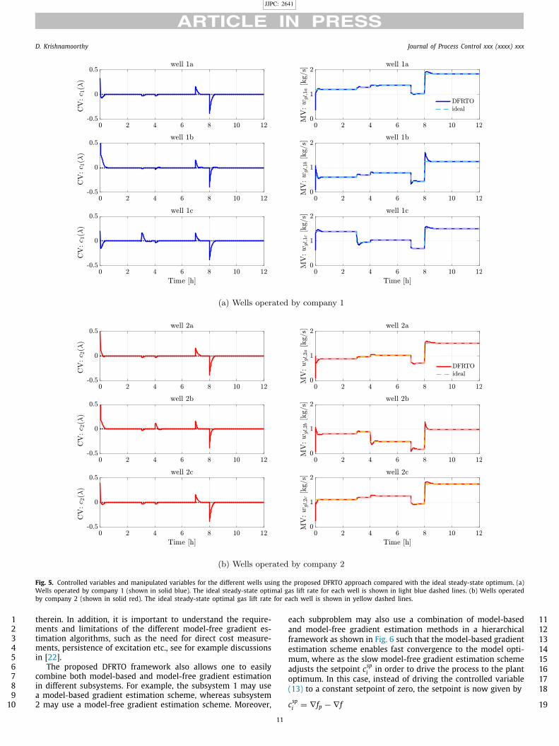
The controlled variables c1(�) and c2(�), along with the manip-45ulated variables wgl,i for the different wells operated by company461 and company 2 are shown in Figs. 5a and 5b respectively. To47benchmark the performance of the proposed DFRTO approach,48the ideal optimal gas lift rates for the different wells operated49by company 1 and 2 are plotted in dashed lines in Figs. 5a50and 5b respectively. This clearly shows that using the proposed51DFRTO method xi converges to same stationary solution as the52overall optimization problem (26). The controlled variables ci(�)53shown on the left subplots in Figs. 5a and 5b indicates that the54proposed DFRTO method is also able to attain dual feasibility.55The simulation with noise can be found in the supplementary56information.57

4 The models were implemented in MATLAB v.2019b which can be found inthe supplementary information or in https://github.com/dinesh-krishnamoorthy/Industrial-Symbiosis/tree/master/Feedback_DistRTO_AL.

As mentioned earlier, one of the main advantages of the pro- 58posed approach is that it does not need to solve the optimization 59problems online. In the example above, solving each subproblem 60in the traditional ADMM approach incurred a computation cost of 613 orders of magnitude5 compared to using feedback controllers. 62Using ADMM also leads to solving the master and subproblems 63iteratively, further increasing the online computational cost. The 64proposed approach on the other hand does not need to iterate 65between the master problem and the subproblems, and does 66not need to solve numerical optimization problems online. The 67simulation results obtained using ADMM can be found in the 68supplementary information. 69

5. Discussions 70

Section 2.2 presented a distributed feedback-based RTO frame- 71work with a centralized master coordinator, where the different 72subsystems use simple feedback control to drive the process 73to a stationary point of the original optimization problem (3), 74which was also shown using an oil production optimization case 75study in Section 4. The proposed approach is computationally 76fast, since this does not require the need to solve numerical 77optimization problems online. This also enables the feedback 78controllers to be implemented at higher sampling rates than 79traditional model-based RTO. 80

5.1. Constraint feasibility 81

We noted earlier that the proposed framework does not iterate 82between the master and the subproblems unlike the traditional 83distributed RTO framework, since this is done in real time. This 84implies that, like any feedback-based RTO method, the coupling 85constraint may not be feasible during the transients. This was also 86noted in Theorem 1, where primal feasibility is guaranteed only 87upon convergence. However, this is not an issue, since the focus 88here is steady-state real time optimization. 89

Even in the case of traditional distributed steady-state RTO, 90the optimal solution computed iteratively may be primal feasible, 91but this is only provided as setpoints to the lower level regulatory 92controllers. Consecutively, the actual closed-loop trajectory of the 93system itself may not be feasible during the transients until the 94process reaches steady-state. 95

5.2. Choice of self-optimizing controlled variables 96

In the proposed DFRTO framework, we considered the self- 97optimizing controlled variable (13). Using this controlled vari- 98able enables us to analyze under what conditions the proposed 99framework converges to a stationary point. Furthermore, the 100convergence analysis in Section 3 provide guidelines on choos- 101ing the penalty parameter ⇢, which is also used as the step 102length in the dual ascent step in the master coordinator. Alter- 103natively, one can also use the simpler self-optimizing variable 104obtained from the unaugmented Lagrangian (9). Although the 105convergence properties using (9) is not guaranteed, it may work 106well in practice. 107

We also considered the optimal sharing problem of the form 108(3), where the coupling constraints are linear. Although this may 109seem restrictive, a wide range of optimal resource sharing prob- 110lem arising in the process industry can be expressed in this form. 111

5 ⇠0.015 s, as opposed to ⇠ 0.15 ⇥ 10�4 s using a standard 2.6 GHz 16 GBmemory processor.

9

JJPC: 2641

D. Krishnamoorthy Journal of Process Control xxx (xxxx) xxx

Fig. 4. Simulation results of the proposed DFRTO framework. (a) The shadow price � and the residual r that is shared across all the subsystems. (b) The total gaslift rate and the system wide optimal cost obtained using the DFRTO approach (shown in solid black) and the ideal steady-state optimum (shown in dashed gray).(c) The gas–oil-ratio (GOR) from the two reservoir sections, which acts as the feed disturbance.

In the case of additively separable nonlinear coupling constraints1of the form2NX

i=1

gi(xi) = 03

the self-optimizing controlled variable in the proposed DFRTO4framework can be modified as5

ci(�) = rxifi(xi) + rxi

gi(xi)(� + ⇢r)6

where r = Pigi(xi). We now have to estimate the constraint7

gradient rxigi(xi) in addition to the cost gradient.8

In many industrial symbiosis systems, the different subsys-tems must agree upon a common variable, for example, the flowrate of a particular stream from one subsystem to another. Thisleads to a consensus problem, where each subsystem has a localcopy of the common variable, and the master coordinator ensuresthat the local copies of the common variable are equal to theoptimum value. In the case of a consensus problem of the form,

minx0,x1,...

X

i

fi(xi) + fs(x0) (28a)

s.t. xi = x0 8i (28b)

the self-optimizing controlled variables can be given by driving 9the gradient of the augmented Lagrangian of each subproblem to 10a constant setpoint of zero, i.e. 11

ci(�i) = rxifi(xi) + �i + ⇢(xi � x0) 8i 12

The convergence analysis framework presented in Section 3 can 13also be used to provide convergence properties of the feedback- 14based consensus problem with suitable adjustments. 15

5.3. Plant-model mismatch 16

As mentioned earlier, any gradient estimation scheme may 17be used with the proposed DFRTO framework. In Section 4, we 18have used a model-based gradient estimation scheme [30] as- 19suming no structural uncertainty. In the presence of structural 20mismatch, one can alternatively estimate the plant gradients 21directly from the cost measurement in a model-free fashion. 22However, the convergence to the stationary point is significantly 23slower when using a model-free gradient estimation scheme as 24opposed to model-based gradient estimation scheme, as noted 25in several works, see for example [19,22,30] and the references 26

10

JJPC: 2641

D. Krishnamoorthy Journal of Process Control xxx (xxxx) xxx

Fig. 5. Controlled variables and manipulated variables for the different wells using the proposed DFRTO approach compared with the ideal steady-state optimum. (a)Wells operated by company 1 (shown in solid blue). The ideal steady-state optimal gas lift rate for each well is shown in light blue dashed lines. (b) Wells operatedby company 2 (shown in solid red). The ideal steady-state optimal gas lift rate for each well is shown in yellow dashed lines.

therein. In addition, it is important to understand the require-1ments and limitations of the different model-free gradient es-2timation algorithms, such as the need for direct cost measure-3ments, persistence of excitation etc., see for example discussions4in [22].5

The proposed DFRTO framework also allows one to easily6combine both model-based and model-free gradient estimation7in different subsystems. For example, the subsystem 1 may use8a model-based gradient estimation scheme, whereas subsystem92 may use a model-free gradient estimation scheme. Moreover,10

each subproblem may also use a combination of model-based 11and model-free gradient estimation methods in a hierarchical 12framework as shown in Fig. 6 such that the model-based gradient 13estimation scheme enables fast convergence to the model opti- 14mum, where as the slow model-free gradient estimation scheme 15adjusts the setpoint csp

iin order to drive the process to the plant 16

optimum. In this case, instead of driving the controlled variable 17(13) to a constant setpoint of zero, the setpoint is now given by 18

csp

i= rfp � rf 19

11

JJPC: 2641

D. Krishnamoorthy Journal of Process Control xxx (xxxx) xxx

Fig. 6. The proposed DFRTO framework using both model-based and model-freegradient estimation to handle plant-model mismatch.

where rfp is the plant gradient estimated directly from the cost1measurement and rf is the model-gradient.2

This is similar to the idea used in modifier adaptation (MA)3scheme for RTO [41], where the term (rfp � rf ) is the so-4called modifier, and instead of using the modifier in the numerical5optimization problem, it can be used to “modify” the setpoint6used in the feedback controller as shown in Fig. 6.7

5.4. Methodology agnostic approach8

Perhaps most intriguingly, the proposed framework enables a9methodology agnostic approach, where different RTO tools may10be used by the different subsystems, truly enabling industrial11symbiosis. For example, currently the distributed RTO frame-12work requires that the all the subproblems are solved using13the traditional model-based RTO approach. However, in an in-14dustrial symbiosis with different organizations, one organization15may wish to use a traditional model-based RTO, whereas an-16other organization may prefer to use simple feedback controllers,17while another organization prefers to use a purely data-driven18approach. Lack of consensus between the different organizations19on the RTO tool impedes successful industrial symbiosis.20

Since the centralized coordinator used in the proposed ap-21proach is the same as the one used in the traditional distributed22RTO, this enables the use of traditional distributed RTO along23with the feedback-based distributed RTO, such that some of the24subproblems are solved numerically, while others using feedback25control. Furthermore, as mentioned earlier, both model-based26and model-free data-driven approaches can be used simulta-27neously with the proposed framework. This is a natural and28interesting research direction that would enable co-ordination29among the different subsystems without imposing strict require-30ments on the RTO methodology in order to establish a centralized31coordinator.32

6. Conclusion33

This paper proposed a distributed feedback-based online pro-34cess optimization framework for optimal resource sharing prob-35lems without the need to solve numerical optimization problems36online. We proposed a local self-optimizing variable for each sub-37system (13) expressed as a function of the shadow price, which38can be controlled to a constant setpoint of zero using simple39feedback controllers. As the centralized master coordinator (14)40updates the shadow price to reach market equilibrium, this leads41to a stationary point of the overall system. Theorem 1 showed42that the proposed DFRTO framework is guaranteed to converge43

to a stationary point of the system, which is often also optimal 44in many applications. The proposed approach was demonstrated 45using a subsea oil and gas production optimization case example. 46

CRediT authorship contribution statement 47

Dinesh Krishnamoorthy: Conceptualization, Methodology, 48Software, Validation, Formal analysis, Investigation, Writing - 49original draft, Writing - review & editing. 50

Declaration of competing interest 51

The authors declare that they have no known competing finan- 52cial interests or personal relationships that could have appeared 53to influence the work reported in this paper. 54

Appendix A. Supplementary data 55

56Supplementary material related to this article can be found 57online at https://doi.org/10.1016/j.jprocont.2020.11.006. 58

References 59

[1] S. Wenzel, R. Paulen, G. Stojanovski, S. Krämer, B. Beisheim, S. Engell, Opti- 60mal resource allocation in industrial complexes by distributed optimization 61and dynamic pricing, At-Automatisierungstechnik 64 (6) (2016) 428–442. 62

[2] S. Boyd, L. Xiao, A. Mutapcic, J. Mattingley, Notes on decomposition 63methods, Notes for EE364B, Stanford University, 2007, pp. 1–36. 64

[3] J.M. Maestre, R.R. Negenborn, et al., Distributed model predictive control 65made easy, Vol. 69, Springer, 2014. 66

[4] R.A. Jose, L.H. Ungar, Pricing interprocess streams using slack auctions, 67AIChE J. 46 (3) (2000) 575–587. 68

[5] R. Martí, D. Navia, D. Sarabia, C. De Prada, Shared resources management 69by price coordination, in: Computer Aided Chemical Engineering, Vol. 30, 70Elsevier, 2012, pp. 902–906. 71

[6] V. Gunnerud, B. Foss, Oil production optimization—A piecewise linear 72model, solved with two decomposition strategies, Comput. Chem. Eng. 34 73(11) (2010) 1803–1812. 74

[7] G. Stojanovski, L. Maxeiner, S. Krämer, S. Engell, Real-time shared resource 75allocation by price coordination in an integrated petrochemical site, in: 762015 European Control Conference (ECC), IEEE, 2015, pp. 1498–1503. 77

[8] D. Krishnamoorthy, C. Valli, S. Skogestad, Real-time optimal resource al- 78location in an industrial symbioticnetwork using transient measurements, 79in: Proceedings of the 2020 American Control Conference, IEEE, 2020, pp. 803541–3546. 81

[9] T. Goldstein, B. O’Donoghue, S. Setzer, R. Baraniuk, Fast alternating 82direction optimization methods, SIAM J. Imaging Sci. 7 (3) (2014) 831588–1623. 84

[10] B. Houska, D. Kouzoupis, Y. Jiang, M. Diehl, Convex optimization with 85aladin, Math. Program. (2018). 86

[11] D. Krishnamoorthy, B. Foss, S. Skogestad, Steady-state real-time opti- 87mization using transient measurements, Comput. Chem. Eng. 115 (2018) 8834–45. 89

[12] M.L. Darby, M. Nikolaou, J. Jones, D. Nicholson, RTO: An overview and 90assessment of current practice, J. Process Control 21 (6) (2011) 874–884. 91

[13] D. Shook, Best practices improve control system performance, Oil Gas J. 92104 (38) (2006) 52. 93

[14] M.G. Forbes, R.S. Patwardhan, H. Hamadah, R.B. Gopaluni, Model predictive 94control in industry: Challenges and opportunities, IFAC-PapersOnLine 48 95(8) (2015) 531–538. 96

[15] K. Forsman, Implementation of advanced control in the process industry 97without the use of mpc, IFAC-PapersOnLine 49 (7) (2016) 514–519. 98

[16] M. Morari, Y. Arkun, G. Stephanopoulos, Studies in the synthesis of control 99structures for chemical processes: Part i: Formulation of the problem. 100Process decomposition and the classification of the control tasks. Analysis 101of the optimizing control structures, AIChE J. 26 (2) (1980) 220–232. 102

[17] S. Skogestad, Plantwide control: the search for the self-optimizing control 103structure, J. Process Control 10 (5) (2000) 487–507. 104

[18] B. Chachuat, B. Srinivasan, D. Bonvin, Adaptation strategies for real-time 105optimization, Comput. Chem. Eng. 33 (10) (2009) 1557–1567. 106

[19] B. Srinivasan, D. Bonvin, 110th anniversary: A feature-based analysis of 107static real-time optimization schemes, Ind. Eng. Chem. Res. 58 (31) (2019) 10814227–14238. 109

[20] S. Engell, Feedback control for optimal process operation, J. Process Control 11017 (3) (2007) 203–219. 111

12

JJPC: 2641

D. Krishnamoorthy Journal of Process Control xxx (xxxx) xxx

[21] J. Jäschke, Y. Cao, V. Kariwala, Self-optimizing control–a survey, Annu. Rev.1Control (2017).2

[22] G. François, B. Srinivasan, D. Bonvin, Comparison of six implicit real-3time optimization schemes, J. Eur. Syst. Autom. 46 (EPFL-ARTICLE-170545)4(2012) 291–305.5

[23] S. Menta, A. Hauswirth, S. Bolognani, G. Hug, F. Dörfler, Stability of dynamic6feedback optimization with applications to power systems, in: 2018 56th7Annual Allerton Conference on Communication, Control, and Computing8(Allerton), IEEE, 2018, pp. 136–143.9

[24] A. Hauswirth, A. Zanardi, S. Bolognani, F. Dörfler, G. Hug, Online optimiza-10tion in closed loop on the power flow manifold, in: 2017 IEEE Manchester11PowerTech, IEEE, 2017, pp. 1–6.12

[25] S. Boyd, N. Parikh, E. Chu, B. Peleato, J. Eckstein, Distributed optimization13and statistical learning via the alternating direction method of multipliers,14Found. Trends Mach. Learn. 3 (1) (2011) 1–122.15

[26] H. Uzawa, Walras’ tatonnement in the theory of exchange, Rev. Econom.16Stud. 27 (3) (1960) 182–194.17

[27] G. François, B. Srinivasan, D. Bonvin, Use of measurements for enforcing18the necessary conditions of optimality in the presence of constraints and19uncertainty, J. Process Control 15 (6) (2005) 701–712.20

[28] M. Krsti¢, H.-H. Wang, Stability of extremum seeking feedback for general21nonlinear dynamic systems, Automatica 36 (4) (2000) 595–601.22

[29] K.B. Ariyur, M. Krstic, Real-time optimization by extremum-seeking23control, John Wiley & Sons, 2003.24

[30] D. Krishnamoorthy, E. Jahanshahi, S. Skogestad, A feedback real time25optimization strategy using a novel steady-state gradient estimate and26transient measurements, Ind. Eng. Chem. Res. 58 (2019) 207–216.27

[31] V. Kumar, N. Kaistha, Hill-climbing for plantwide control to economic 28optimum, Ind. Eng. Chem. Res. 53 (42) (2014) 16465–16475. 29

[32] M. Hong, Z.-Q. Luo, M. Razaviyayn, Convergence analysis of alternating 30direction method of multipliers for a family of nonconvex problems, SIAM 31J. Optim. 26 (1) (2016) 337–364. 32

[33] X. Zhou, On the fenchel duality between strong convexity and lipschitz 33continuous gradient, 2018, arXiv preprint arXiv:1803.06573. 34

[34] Equinor, Long life at norne, 2015, URL https://www.equinor.com/en/news/ 352015/01/09/article.html. 36

[35] V. Gunnerud, B. Foss, B. Nygreen, R. Vestbø, N.C. Walberg, Dantzig-wolfe 37decomposition for real-time optimization-applied to the troll west oil rim, 38IFAC Proc. Vol. 42 (11) (2009) 69–75. 39

[36] D. Krishnamoorthy, K. Fjalestad, S. Skogestad, Optimal operation of oil and 40gas production using simple feedback control structures, Control Eng. Pract. 4191 (2019) 104107. 42

[37] D. Krishnamoorthy, E. Jahanshahi, S. Skogestad, Gas-lift optimization 43by controlling marginal gas-oil ratio using transient measurements, 44IFAC-PapersOnLine 51 (8) (2018) 19–24. 45

[38] D. Krishnamoorthy, S. Skogestad, Online process optimization with active 46constraint set changes using simple control structures, Ind. Eng. Chem. Res. 47(2019). 48

[39] A.C. Hindmarsh, P.N. Brown, K.E. Grant, S.L. Lee, R. Serban, D.E. Shumaker, 49C.S. Woodward, Sundials: Suite of nonlinear and differential/algebraic 50equation solvers, ACM Trans. Math. Softw. (TOMS) 31 (3) (2005) 363–396. 51

[40] A. Wächter, L.T. Biegler, On the implementation of an interior-point 52filter line-search algorithm for large-scale nonlinear programming, Math. 53Program. 106 (1) (2006) 25–57. 54

[41] A. Marchetti, B. Chachuat, D. Bonvin, Modifier-adaptation methodology for 55real-time optimization, Ind. Eng. Chem. Res. 48 (13) (2009) 6022–6033. 56

13