A Digital Twin-Driven Method for Online QualityControl in Process IndustryXiaoyang Zhu 

Zhejiang UniversityYangjian Ji  ( mejyj@zju.edu.cn )

Zhejiang University

Research Article

Keywords: Digital twin, Online quality control, Process industry, Bidirectional gated recurrent unit,Attention mechanism, Improved genetic algorithm

Posted Date: June 3rd, 2021

DOI: https://doi.org/10.21203/rs.3.rs-571586/v1

License: This work is licensed under a Creative Commons Attribution 4.0 International License.  Read Full License

Version of Record: A version of this preprint was published at The International Journal of AdvancedManufacturing Technology on January 5th, 2022. See the published version athttps://doi.org/10.1007/s00170-021-08369-5.

A Digital Twin-Driven Method for Online Quality Control in

Process Industry

Xiaoyang Zhu1, 2, 3 • Yangjian Ji1, 2, 3 *

Abstract

To ensure the stability of product quality and production continuity, quality control is drawing increasing attention from the process industry. However, current methods cannot meet requirements with regard to time series data, high coupling parameters, delayed data acquisition and ambiguous operation control. A digital twin-driven (DTD) method for real-time monitoring, evaluation and optimization of process parameters that are strongly related to product quality is proposed. Based on a process simulation model, production status information and quality related data are obtained. Combined with an improved genetic algorithm (GA), a time sequential prediction model of bidirectional gated recurrent unit (bi-GRU) with attention mechanism (AM) is built to flexibly allocate parameter weights, accurately predict product quality, timely evaluate technical process and rapidly generate optimized control plans. A typical case study and relevant filed tests from the process industry are presented to prove the effectiveness of the method. Results indicate that the proposed method clearly outperforms its competitors.

Keywords Digital twin · Online quality control · Process industry · Bidirectional gated recurrent unit · Attention mechanism · Improved genetic algorithm

1. Introduction

Process industries are those that add value to raw materials by mixing, separating, heating, molding or chemical reactions. Production of process industries is generally continuous or in batch and requires strict process control as well as safety measures. Featuring relatively fixed process, high energy consuming, few product specifications and large production scale, the process industry mainly covers petroleum, chemical, metallurgy, food, pharmaceutical, optical fiber, cement, etc [1].

Product quality is one of the two most important issues in modern industry [2]. The process industry is even more urgently in need of research about product quality control than others. Technical processes in process industries are typically continuous and irreversible, inevitably leading to quality problem accumulation [3]. Given large-scale production, frequent quality issues can dramatically increase the total cost of a factory. In some extreme cases, there may be catastrophic losses such as equipment damage, environmental pollution or even casualties [4].

Compared to the discrete industry, main obstacles to achieving quality control in the process industry include: (1) Accompanied by multiple physical and chemical reactions, ingredients and attributes of raw materials during production are changeable and unpredictable. As a result, it is hard to

*Yangjian Ji mejyj@zju.edu.cn

13034207089

Xiaoyang Zhu

ORCID：0000-0003-4806-7573

1 The authors are with State Key Laboratory of Fluid Power and Mechatronic Systems, Zhejiang University, Hangzhou, Zhejiang 310027, PR China. 2 The authors are with Key Laboratory of Advanced Manufacturing Technology of Zhejiang Province, Zhejiang University, Hangzhou, Zhejiang 310027, PR China. 3 The authors are with Department of Industrial and System Engineering, Zhejiang University, Hangzhou, Zhejiang 310027, PR China.

describe the whole process with precise mathematical models. (2) Processing environment is often extreme conditions such as high temperature and high pressure [5]. It enhances the difficulty for existing sensors to timely and accurately measure quality data [6]. (3) Highly coupled technical parameters turn quality control into a multi-scale, multi-process and multi-objective dynamic conflicting optimization. (4) Setting and adjustment of parameters still heavily rely on existed experience [7]. Different operator proficiency levels and unforeseen accidental errors may exert considerable influences on product quality consistency. (5) Quality problems tend to accumulate during continuous production, but technologists are impossible to conduct quality tests all the time. In summary, research on online quality control in the process industry is an important way to achieve goals of increasing yields, shortening processing time, reducing costs, ensuring high product quality and protecting the safety of equipment and personnel.

With the deepening of quality control research, related models and processes have been improved. And yet, current methods are still poor in timeliness and intelligence, leading to a lack of predictability, instant feedback and decision-making capability in quality data. Application demands and technical requirements of modern manufacturing technologies in different fields are constantly rising. In consequence, online control and effective improvement of product quality become a problem demanding prompt solution. This paper proposes a digital twin-driven method for online quality control, aiming to control technical process in real time, reduce human intervention, improve product quality and ensure its stability.

The remainder of this paper is organized as follows. Research about quality control in process industries and applications of digital twin are reviewed in Section 2. Section 3 details the theoretical frame of the proposed DTD online quality control. Operation mechanism and implementation procedure of the proposed method are reported in Section 4. In Section 5, a case about optical fiber preform drawing process is presented for validation, and Section 6 draws concluding remarks.

2. Related work

2.1 Quality control in process industries

There are currently four main ideas for product quality control in the process industry: (1) To replace hardware instruments or assist in offline analysis with soft sensors [8], and then use empirical control to obtain optimized process parameters. (2) To identify abnormal fluctuations in the production through various improved control charts to guarantee product quality[9]. (3) To acquire the relationship between process parameters and product quality [10] through association rule mining or filed tests, use intelligent optimization algorithms to help compile or adjust rules and achieve the optimization of product quality. (4) The mixed use of above methods. Universally used in process monitoring and fault diagnosis, a soft sensor is the association of a sensor with an estimation algorithm, which makes online measurements of certain process variables possible [11 ]. Soft sensors are generally divided into two types, model-driven and data-driven. The former is commonly based on the first principle model but hard to be extensively used on account of its complicated processes and unquantifiable parametric relationships. The most popular modeling techniques for data-driven soft sensors include principal component regression (PCR) [12, 13], partial least squares (PLS) [14, 15], artificial neural networks (ANN) [16, 17] and support vector machines (SVM) [18, 19]. Wang et al. [20] integrated random forest with Bayesian optimization to predict and maintain product quality and validated model superiorities through semiconductor production line data. Li et al. [21] presented a distributed SVM based soft sensor to online measure the digested slurry quality and optimized the raw material proportioning through expert knowledge. The drawback of soft sensor method is that optimization or adjustment of parameters is highly dependent on process background knowledge and universally short of effect verification. Control charts are powerful tools which are frequently used to monitor processing, detect unusual variation and help technicists quickly response by plotting statistics computed from a random process sample [22]. Chen et al. [23] built a recurrent neural network model to characterize variables at time lags in process industries and developed a residual control chart to detect mean shifts in autocorrelated processes. For multi-stage manufacturing processes, Asadzadeh et al. [24] proposed a cumulative sum control chart and an exponentially weighted moving average control chart to monitor quality variables in terms of effective covariates. Nonetheless, the establishment of control charts and various self-adaptive improvements are largely derived from process models and data features of specific industries. The strong particularity results in the poor reproduction ability in other fields.

Intelligent optimization algorithm is a kind of random search evolution algorithm. Lee et al. [25]

utilized the hybridization of fuzzy association rule mining and variable-length slippery GA to determine process parameter settings and improve finished quality of garment manufacturing. Kramar et al. [26] developed a particle swarm optimization based fuzzy expert system to predict mechanical properties of molded parts, obtained optimal process parameters and effectively improved the injection molding quality. However, the association rules used to set relevant parameters in the optimization process are mostly based on the historical data analysis, making it hard to guide quality data prediction in time and later process decision-making.

2.2 Digital twin

The concept of digital twin was first introduced by Grieves [27] around 2003 during his presentation, who regarded it as a conceptual idea for product lifecycle management. Until 2010, the term "Digital Twin" was formally proposed in NASA's technical reports and the technology was intensively applied in aerospace fields thereafter. In recent years, with the advancement of big data processing and analysis capability, cloud computing technology [28], artificial intelligence technology [29], simulation modeling theory [30], optimization algorithm [31], as well as availability and usability of massive industrial data, digital twin technology has been developed and widely used in both academia and industry [32].

Tao et al. [33] described digital twin as an interdisciplinary technique, which makes full use of models, data and intelligence to serve as a bridge connecting physical world and information world, providing more real-time, efficient and comprehensive services. It shows outstanding performances in condition monitoring[34 , 35 ], behavior evaluation [36 , 37 ], control guidance [38 , 39 ] and overall optimization during the entire life cycle [40, 41] of a component, a product or a system.

The construction of a digital twin system can realize parallel operation, real-time interaction and iterative optimization of industrial entities and virtual twins. Accurate prediction and adjustment, self-organizing and optimized scheduling, equipment lifecycle management, product quality traceability and control are achieved. It greatly improves production quality and efficiency, and further, effectually promotes the rapid development of the process industry. With the data-driven digital twin, He et al. [42] developed an adaptive subspace identification method to achieve optimal control of process systems, thereby ensuring stability and controllability of product quality with device abnormalities. Lee et al. [43] studied the application of cyber-physical production systems in metal castings, updated production status in real time through quality inspection model, issued an alarm when the defect rate exceeded standards, and made corrections to production plans. In the ore waste phosphorus processing, Dli et al. [44 ] combined process mechanism model and deep neural network model to construct a digital twin model for product quality control and energy consumption optimization.

To conclude, digital twin technology provides a new idea for the online control of product quality in the process industry, but there are few related studies at present. This paper combines digital twin and artificial neural network to online monitor production and predict product quality. Optimized parameters are obtained from the improved intelligent optimization algorithm, validated in simulation models and fed back to physical systems. Production process and product quality are therefore kept stable.

3. Theoretical Framework for DTD Online Quality Control

This research aims to apply digital twin technology to online product quality control in the process industry. Based on physical-virtual mapping, production information processing and fused data related to quality control, the theoretical framework for DTD online quality control is established.

Fig. 1 Theoretical framework for DTD online quality control

As shown in Fig. 1, the framework structure comprises physical production system, virtual production system, central control system, twin data and mechanism library. Every system is equipped with multiple open interfaces for digitization, automation and visualization. Good compatibility and scalability, along with a set of standard data communication and conversion devices, facilitate perceptual access and efficient integration of multi-source heterogeneous data.

3.1 Physical production system

The physical production system is an on-site production center composed of equipment, operators, environment and processing objects, responsible for receiving production tasks from the central control system and executing production activities. Detailed production instructions are pre-defined according

to the simulation and optimization in the virtual production system. Benefit from the intelligent perception system, mass data during the production can be collected in real time [45]. Working conditions, therefore, could be monitored dynamically, evaluated timely and adjusted precisely under any disturbances. Compared with traditional production centered on human decision-making, the physical production system possesses a better flexibility, adaptability, robustness and intelligence.

3.2 Virtual production system

The virtual production system is a vivid mapping of the physical production system according to physical description and behavioral expression of production elements. The mechanism model is used for decoupling analysis of the relationship between variables and indicators to guide the simulation model construction. The data model is built from filtered and stored historical processing data to support product quality control. Main functions of the system are as follows: reasonable abstraction of production process; conditions idealization of physical entity attributes; precise setting of process parameters; simulation and visualization of the physical production system, as well as verification and evaluation of process parameters combination provided by the central control system. In summary, before the production, the virtual production system simulates and analyzes production plans to identify potential risks. During the production, it accurately depicts and realistically displays sequence, concurrency and connectivity of production activities. At the end of the production, plenty of product quality related data will be generated to feed back the central control system to decide whether to follow or revise production plans.

3.3 Central control system

As the core of the production digital twin, the central control system directly determines degree of intelligence and precision of quality control. The system involves four parts: (1) Data acquisition and processing system. With precise control of working conditions, timely transmission of production status data and seamless connection of networks, an information center is constructed. It is composed of network facilities, terminal equipment and application softwares, in support of production monitoring and management. (2) Two-way mapping physical-virtual production system. The virtual system simulates elements, behaviors and rules in the physical system so as to truly reproduce it. On the contrary, the physical system follows simulated and validated production plans in the virtual system. Two systems interact in real time to grasp changes and make responds dynamically, thereby continuously optimizing production process. (3) Product quality prediction system. Historical data constitute a working condition library to make preliminary judgments of current status. The product quality is further predicted based on collected data from the past and the future. (4) Dynamic parameter optimization system. Adjustments are performed based on the difference between predicted results and tolerance requirements. The data representing working condition at the previous moment is used as the input of optimization algorithm at the next moment. Sequentially, optimal results are verified iteratively in the virtual production system until suitable for actual operations. In general, the central control system is responsible for providing system support and services for real-time control driven by product quality twin data.

3.4 Quality control twin data

The quality control twin data is the collection of fused data generated and transferred in systems, which directly or indirectly determines final product quality. Twin data mainly includes: (1) Design data, technological data and process data pre-defined according to production plans before everything starts. (2) Real-time collected data, mainly about environmental conditions, object attributes, equipment status and production progress. (3) Virtual simulation data, mainly including driving data, model data, prediction data, analysis data, decision data, etc. (4) Fused data derived from integration, counting, correlation, clustering, evolution, regression and generalization of real-time collected data and virtual simulation data. (5) Historical data acquired in past technical processes. Overall, twin data provides a data collection and sharing platform for the production [46], eliminating information islands. On the basis of integration and fusion, twin data keeps updating and expanding, which is the driven force to achieve the normal operation of all constituent systems as well as pairwise interactions.

3.5 Mechanism library

The mechanism library is responsible for unified management, explanation and adjustment of various trigger, interaction and control modes during the system operation. Its main components include

mapping rule, information communication mechanism, feedback transmission mode and twin data fusion form between systems. The mechanism library formulates operating rules of the entire digital twin system according to actual needs and ensures its smooth and efficient operation.

4. Operation Mechanism for DTD Online Quality Control

4.1 System operation process

The flow chart of system operation is shown in Fig. 2. After production tasks are released, the central control system will automatically generate production plans. The virtual production system will simulate and evaluate the production plan in advance to ensure its feasibility and introduce it into the physical production system. Technicians operate equipment to launch the production. The physical and the virtual production systems come into operation and constantly interact with each other, while the data generated from systems keep flowing. Both real-time collected data and simulation data will be integrated and stored in the central control system. Before then, there will be a filtering and verification step to pre-check that these data are within normal parameter ranges.

Next, all the data related to quality control will be imported into the product quality prediction system to assist the central control system in prediction and decision-making. If predicted results meet tolerance requirements, it is decided according to production progress data to end or continue the production. Otherwise, the dynamic optimization system is actuated. Similarly, optimized and adjusted parameters will be simulated and evaluated in the virtual production system beforehand, and, if feasible, imported into the physical production system to guide operations. The physical and the virtual production systems are still able to resume synchronization and keep interaction after adjustments. To update and optimize the working condition library, the adjusted data will be retained in place of the original.

During the whole process, above mentioned online quality control procedures will be carried out iteratively until the central control system declares that predicted results meet tolerance requirements based on current working conditions and announces the completion of the production task.

Finally, the physical and the virtual production system will further perform the data processing with integration, supplement, replacement and analysis so as to feed back the central control system to follow or amend production plans. The feedback could improve the quality of process design, thus enabling the digital twin system to maintain self-learning and self-optimization.

Fig. 2 Flow chart of system operation process

4.2 Real-time data acquisition

A huge amount of real-time industrial data related to product quality serves as an important resource for evaluating the completion of processing tasks. Data perception and processing are important steps to obtain effective product quality related data [47]. As shown in Fig. 3, real-time data acquisition of industrial process contains four layers: physical entity, data transmission, data processing and data sensing. First of all, a complete sensor system that matches production, monitoring and logistics equipment is deployed. The sensor network provides hardware support for data collection. Through Wi-Fi, Bluetooth, mobile network, communication protocols (Modbus, TCP/IP) and industrial Internet (Ethernet, Passive Optical Network), the data transmission can be stable and efficient with a low loss. Multi-source heterogeneous data undergoes operations such as conversion, classification, analysis, calculation and fusion, and will eventually transforms to effective and usable sources available for quality prediction and production decision-making. The information in the sensed data mainly contains: size (length, width, height), material (solid, liquid, gas), state (deformation, phase change) and attribute (batch, number, requirement) of processed objects; operation related information, such as process (sequence, position, time), parameter (velocity, current, voltage) and progress (start, downtime, abnormal); environment description, such as temperature, humidity and pressure intensity; energy consumption condition, such as electricity, coal and water.

Fig. 3 Real-time data acquisition of industrial process

4.3 Process simulation model

As a basis of digital twin, a complete process simulation model should involve the following contents: qualitative analysis, parameter import, attribute configuration and visual interface. Fig. 4 shows

system architecture of a finite element simulation model for glass hot forming, a typical technical process of the process industry.

Fig. 4 System architecture of finite element simulation model

4.3.1 Qualitative analysis

According to technical processes and simulation requirements, the first step is to determine whether to conduct stationary or time dependent research, and model dimensionality. Then, boundary coordinate system, possible processing domains and different deformation effects are to be defined. The most decisive step is to choose suitable physics interfaces required for the simulation and to solve cyclic coupling problems that may occur between different physical fields.

4.3.2 Parameter import

Parameters to import models mainly include: geometric parameters, mainly consisting of original and expected object dimensions, main reaction areas, contact positions of machine and object, special monitoring points and other elements; material parameters, such as density, dynamic viscosity, thermal conductivity, specific heat rate, constant pressure heat capacity, surface emission rate, surface tension coefficient and Poisson’s ratio; process parameters, mainly referred to time series of parameters that directly affect product quality; environment parameters, such as ambient temperature, humidity and atmospheric pressure; default parameters, defined according to different scenarios and process variables.

4.3.3 Attribute configuration

An important idea of finite element simulation is to merge individual properties of lots of tiny elements to form overall object properties, which relies much on meshes. Division, attribute definition and mutual coordination of mesh are the most significant guarantee for accuracy and timeliness of the entire simulation process. The design of simulation steps also plays a critical role. Besides, detailed solver configuration should be carried out, including equation compilations, dependent variable settings and special parameter settings.

4.3.4 Visual interface

To control technical process and product quality in real-time, a nice visual interface is indispensable. For one thing, visual displays demand high-fidelity simulation of processes, which is used to assist technicists to observe processing, test the effectiveness of optimization control instructions and obtain change trends of key technical indicators. For another, a user-friendly interface is required to quickly adjust process parameters, feedback simulation information timely, evaluate simulation results and write other instructions. In order to support construction and operation of digital twin, the visual interface should also display the real-time processing status of the physical production system connected with a specific interface.

4.4 Product quality prediction model

4.4.1 Gated recurrent unit

Continuous production of the process industry generates massive time series data. Recurrent neural network (RNN) is a deep model used to learn programs that mix sequential and parallel information [48]. Its basic recurrent units are chained and recursed according to sequence output time. Input parameters are shared and historical data are memorized among units. Therefore, it is suitable to learn nonlinear features implicit in the input sequence.

However, an excessively deep network leads to problems like gradient explosion and gradient disappearance and thus has difficulty in accurately describing current state. To solve the problem, long short term memory (LSTM) [49], as an improved algorithm of RNN, is proposed. A typical LSTM model is composed of input gate, output gate and forget gate. Instead of updating weights with continuous multiplication in RNN, LSTM models adopt continuous addition, avoiding gradient disappearance theoretically. The gradient explosion problem is also settled with gradient clipping. Besides, with more computing units in hidden layers, the nonlinear feature processing capability of LSTM is greatly enhanced. Faced with time series characterized by long time spans, intervals and delays, it is capable of

collecting scattered feature information and compensating insufficient long-term memory ability of RNN. Similarly, if the time span is too long or the network is too deep, LSTM also performs poorly with

huge computation amount and time consuming. An improved variant of LSTM, gated recurrent unit (GRU) [50], is then studied and put into application. GRU model merges input gate and forget gate in original LSTM units into update gate, changes output gate to reset gate, and puts unit state into hidden layer state. It can not only selectively memorize important information and periodically forget the useless, but also keeps a simpler structure than LSTM models. When processing the same data, GRU models use fewer units and faster time under the premise of ensuring accuracy, which saves considerable resources especially when dealing with large-scale data. The structure of GRU is shown in Fig. 5.

Fig. 5 GRU structure

where 𝐱𝑡 is input at time t; 𝒉𝑡 and 𝒉𝑡−1 are hidden states at time t and t-1; 𝒓𝑡 and 𝒛𝑡 are outputs of reset gate and update gate, and 𝒓𝑡 , 𝒛𝑡 ∈ [0,1]𝐷 where D is input dimension; �̃�𝑡 is candidate current state; red circle is sigmoid function; blue circle is hyperbolic tangent function; black circles are element-wise multiplication, element-wise addition and subtraction of previous number from 1. The reset gate determines how to combine new input information with previous memories, which comprises 𝒉𝑡−1 and 𝐱𝑡. 𝒓𝑡 = 𝜎(𝑾𝑟𝒙𝑡 + 𝑼𝑟𝒉𝑡−1 + 𝒃𝑟) (1)

The update gate controls how much information from the previous hidden state will carry over to the current hidden state. 𝒛𝑡 = 𝜎(𝑾𝑧𝒙𝑡 + 𝑼𝑧𝒉𝑡−1 + 𝒃𝑧) (2) Candidate current state is expressed as:

�̃�𝑡 = tanh (𝑾ℎ𝒙𝑡 + 𝑼ℎ(𝒓𝑡⊙𝒉𝑡−1) + 𝒃ℎ) (3) Hidden states at time t is expressed as: 𝒉𝑡 = (1 − 𝒛𝑡) ⊙ �̃�𝑡 + 𝒛𝑡 ⊙𝒉𝑡−1 (4) Where U and W are weight matrices and b is bias, which are parameters to be learned. When 𝒛𝑡 = 0 and 𝒓𝑡 = 1, GRU network degenerates to a simple RNN. When 𝒛𝑡 = 0 and 𝒓𝑡 = 0, current hidden state 𝒉𝑡 is only related to current input 𝐱𝑡 and irrelated to previous hidden state 𝒉𝑡−1. When 𝒛𝑡 = 1, current hidden state 𝒉𝑡 equals previous hidden state 𝒉𝑡−1 and has nothing to do with current input 𝐱𝑡.

4.4.2 Attention mechanism

In view of inherent characteristics of the process industry, unpredictable conditions, such as machine starting or shutdown, parameter adjustment, raw material changes and plan reschedule, arise inevitably during the production. Under different circumstances, degree of parameter influences on product quality is not exactly the same. If influencing weights are not adaptively redistributed according to different sources of change, it is hard to accurately predict product quality. About this issue, attention mechanism (AM) is introduced [51]. Attention mechanism originates from simulation of human brain. As a resource allocation method, it helps to utilize limited computing resources to process more important information, thereby improving efficiency of neural networks. Generally, input information can be expressed in a key-value pair format, where "key" is used to calculate attention distribution, namely the probability of each input vector being selected, while "value" is used to calculate aggregate information. It is necessary to determine a prediction task related representation called query vector, and use a scoring function to calculate the similarity between each input vector and query vector. Fig. 6 shows steps for obtaining attention values.

The input information with N sets of key-value pair at time t is expressed as: (𝑲𝑡 , 𝑽𝑡) = [(𝒌𝑡1, 𝒗𝑡1),···, (𝒌𝑡𝑁, 𝒗𝑡𝑁)] (5)

Fig. 6 AM structure

Step 1 Calculate the similarity between key 𝒌𝑡𝑛 and query vector 𝒒 through scoring function to obtain the correlation between input feature and product quality at the current moment. The attention score is based on input feature 𝐱𝑡𝑛 at the current moment, hidden state 𝒉𝑡−1 and feature attention weight α𝑡−1,𝑛 at the previous moment. Scaled dot product model is used to solve large variance in high dimensional situations: s(𝒌𝑡𝑛, 𝐪) = F(𝒙𝑡𝑛, 𝒉𝑡−1, 𝛼𝑡−1,𝑛) = 𝒌𝑡𝑛𝑇 𝒒√𝐷 (6)

Step 2 Use softmax formula to convert the correlation into a probability form. The probability that the n-th feature is selected at time t is: 𝛼𝑡𝑛 = 𝑝(𝑧 = 𝑛|𝑲𝑡 , 𝒒) = 𝑠𝑜𝑓𝑡𝑚𝑎𝑥(𝑠(𝒌𝑡𝑛, 𝒒)) = exp(𝑠(𝒌𝑡𝑛,𝒒))∑ exp(𝑠(𝒌𝑡𝑗,𝒒))𝑁𝑗=1 (7)

Step 3 Each probability value is multiplied with the implicit representation of the corresponding feature to quantified its contribution to predicted product quality. The sum of contributions of all input features is the input of quality prediction. The predicted input after AM weight redistribution is: 𝒙𝑡 = 𝑎𝑡𝑡((𝑲, 𝑽), 𝒒) = ∑ 𝛼𝑡𝑛𝒗𝑡𝑛𝑁𝑛=1 (8)

where D is the key dimension in the input information; z is the attention variable, used to represent the index position of the selected feature.

4.4.3 Bidirectional gated recurrent unit with attention mechanism

The information in GRU network is transmitted in one direction from front to back, while Bi-GRU can consider both the past and the future data information. The same output is connected to two GRU networks with opposite time flow. The forward GRU is responsible for sequential training to obtain the past data information. The backward GRU performs reverse training to learn features in the future data. At each moment t, hidden state 𝒉𝑡 of bidirectional GRU is jointly determined by forward and backward hidden states.

Forward and backward hidden states are respectively: 𝒉𝑡⃗⃗⃗⃗ = 𝑮𝑹𝑼⃗⃗ ⃗⃗ ⃗⃗ ⃗⃗ ⃗(𝒙𝑡 , 𝒉𝑡−1⃗⃗ ⃗⃗ ⃗⃗ ⃗⃗ ) (9) 𝒉𝑡⃖⃗ ⃗⃗⃗ = 𝑮𝑹𝑼⃖⃗ ⃗⃗ ⃗⃗ ⃗⃗ ⃗⃗ (𝒙𝑡 , 𝒉𝑡+1⃖⃗ ⃗⃗ ⃗⃗ ⃗⃗ ⃗) (10) Current hidden state is: 𝒉𝑡 = 𝑐𝑜𝑛𝑐𝑎𝑡𝑒𝑛𝑎𝑡𝑒(𝒉𝑡⃗⃗⃗⃗ , 𝒉𝑡⃖⃗ ⃗⃗⃗) (11)

where 𝒉𝑡+1⃗⃗ ⃗⃗ ⃗⃗ ⃗⃗ ,𝒉𝑡−1⃖⃗ ⃗⃗ ⃗⃗ ⃗⃗ ⃗are forward state output of moment t+1 and backward state output of moment t-1; 𝒉𝑡⃗⃗⃗⃗ ,𝒉𝑡⃖⃗ ⃗⃗⃗ are forward state output and backward state output at moment t of Bi-GRU network. The model structure of Bi-GRU with AM is shown in Fig .7:

Fig. 7 Bi-GRU with AM

Time sequential quality influencing features, as initial inputs, first go through a series of calculations in attention mechanism. New features, with weights redistributed, then enter Bi-GRU model after vectorization operation. The bidirectional network acquires both the past and the future information of input sequences. At each single moment, forward and backward hidden states are concatenated to form hidden state at the current moment. And further, the predicted quality value sequence is obtained.

4.5 Parameter optimization model

Genetic algorithm (GA) is an efficient heuristic search algorithm developed from genetic evolution of natural populations. Simulating evolutionary phenomenon of the survival of the fittest [52], it maps search space, that is, solution space of problems, into a genetic space, and encodes possible solutions into vectors, generally called a chromosome group. More specifically, a series of initial code strings are randomly generated to form an initial group. Genetic operations are repeatedly performed on previous populations, thereby continuously generating new populations. Each chromosome is evaluated according to fitness value of objective function. The optimal solution that meets requirements under the global parallel search is selected. Genetic algorithm has universality to solve multi-domain problems, simplicity of avoiding derivation or differentiation of objective functions, parallelism for simultaneous comparison of multiple individuals and scalability for combination with other algorithms.

4.5.1 Standard GA

For the optimization of product quality related parameters in the process industry, the difference between actual results and target quality indicators can be used as objective function values. Given some measurable parameters and empirical parameter ranges obtained from historical quality data, an optimized combination of process parameters is generated. Basic operation steps of genetic algorithm are shown below.

Step 1: Determine objective function and solution set. The objective function is preset according to actual needs. The form of solution sets and the effective range of parameters are obtained.

Step 2: Parameter set coding. The solution set to the problem is converted into a chromosome form with a certain coding scheme such as binary or real number coding.

Step 3: Control parameter setting and population initialization. Set key parameters (population size, genetic operation probability, maximum genetic generation, optimization operator, etc.) and randomly generate a series of initial code strings to form the initial population.

Step 4: Population evaluation. Parameter combination after bit string decoding is regarded as individual phenotype, from which objective function values are calculated and mapped to fitness values under certain rules. The fitness of individuals, that is, the ability to adapt to the environment, is then assessed according to the value.

Step 5: Selection operation. The fitness is used as evaluation index to select more adaptable individuals in populations. The greater the fitness value, the greater the probability of individuals being selected. Common selection operators include roulette wheel selection, stochastic tournament, excepted value selection, etc.

Step 6: Crossover operation. Two chromosomes are randomly selected from populations. With one or more crossover points chosen, corresponding genes are exchanged with a certain probability to form a new chromosome.

Step 7: Mutation operation. Caused by some accidental factors, one or a few genes are changed with a certain mutation probability, thus forming a new chromosome.

Step 8: Termination judgement. All populations will be judged by certain rules, on the basis of which it is decided whether the algorithm should stop.

4.5.2 Improved GA

Standard genetic algorithm encounters problems in practical applications: (1) Limited by search ability to new spaces, it is easy to converge to a local optimal solution. (2) Related parameters of genetic operators are set fixed, which may cause a slow convergence. (3) Once best individuals are not inherited and genetic operations fail to produce better individuals, genetic degradation and global optimization performance deterioration tend to occur. (4) With the random optimization inherent, GA is often poor in stability and lacking in screening criteria when multiple optimizations are performed. In response to above problems, this paper proposes an improved genetic algorithm. The structure is shown in Fig. 8 below. Steps of standard genetic algorithm are in green box while six improvements are in blue file box.

Fig. 8 Improved GA structure

Improvement 1: Adaptive crossover rules. The greater the crossover rate, the larger the search space of algorithm and the faster the rate of generating new individuals. At the same time, the possibility of good individuals being destroyed increases. If the crossover rate is too small, it is difficult to generate new individuals and the search process becomes slower. A sigmoid-type function is chosen to describe the adaptive crossover, purposefully imposing a rather high crossover rate to individuals with fitness lower than the average to provide a great search space, and gradually reducing the rate to maintain the inheritance of good individuals as the fitness tends to the maximum. The relevant formulas are as follows:

𝑃𝑐 = { 𝑃𝑐𝑚𝑎𝑥 − 𝑃𝑐𝑚𝑖𝑛1 + exp(𝛼1 (𝑓𝑐 − 𝑓𝑚𝑎𝑥 + 𝑓𝑎𝑣𝑔2 )) + 𝑃𝑐𝑚𝑖𝑛 𝑓𝑐 ≥ 𝑓𝑎𝑣𝑔

𝑃𝑐𝑚𝑎𝑥 𝑓𝑐 < 𝑓𝑎𝑣𝑔 (12) where 𝑃𝑐 , 𝑃𝑐𝑚𝑎𝑥 , 𝑃𝑐𝑚𝑖𝑛 are crossover rate, maximum crossover rate and minimum crossover rate, respectively; 𝑓𝑚𝑎𝑥 and 𝑓𝑎𝑣𝑔 are maximum individual fitness and average individual fitness of the population; 𝑓𝑐 is the larger fitness of two individuals to be crossed; 𝛼1 is a smoothing parameter that adjusts smoothness of the curve. The adaptive crossover rate curve is shown in Fig. 9.

Improvement 2: Adaptive mutation rules. The purpose of introducing mutation in GA is twofold: to possess GA of local random search ability and to maintain group diversity. The greater the mutation rate, the higher the population diversity. But if the mutation rate is too large, the algorithm will become a completely random search algorithm that is unconstrained and difficult to converge. If the rate is too small, the population diversity is limited and the algorithm search space will shrink accordingly. In the early stage of population evolution and in the process of population individual fitness tending to the maximum, it should be ensured that the mutation rate is controlled at a low level but greater than 0 to avoid destroying good individuals. When the individual fitness of the population is close to the average,

the rate should be adjusted to reach the maximum to avoid the algorithm falling into local optimal solutions. A function similar to the normal distribution is chosen to describe the adaptive mutation. The relevant formula is as follows: 𝑃𝑚 = 𝛼2(𝑃𝑚𝑚𝑎𝑥 − 𝑃𝑚𝑚𝑖𝑛)√2𝜋 exp [− (𝑓𝑚 − 𝑓𝑎𝑣𝑔)22 ] + 𝑃𝑚𝑚𝑖𝑛 (13) where 𝑃𝑚 , 𝑃𝑚𝑚𝑎𝑥 , 𝑃𝑚𝑚𝑖𝑛 are mutation rate, maximum mutation rate and minimum mutation rate, respectively; 𝑓𝑚 is fitness of individual to mutate; 𝛼2 is a height parameter of the curve. The adaptive mutation rate curve is shown in Fig. 10.

Fig. 9 Adaptive crossover curve

Fig. 10 Adaptive mutation curve

Improvement 3: Mechanism of eliminating dead and replenishing new individuals. The probability of an individual being selected is positively related to its fitness value. But once the best fitness individual in parent populations is not inherited and crossover or mutation fails to produce a better individual, genetic degradation tends to happen. BestFitness is used to judge whether degradation occurs. Dead individuals are those whose fitness is lower than the average. If BestFitness(n+1) < BestFitness(n), it indicates that contemporary genetic operations have failed to produce better individuals. The elimination mechanism of dead individuals is activated to reduce the probability of genetic degradation. Furthermore, the same number of new individuals are randomly generated to supplement populations in the meanwhile. The replenishing mechanism not only retains current good individuals, but also increases population diversity, expanding search space and enhancing global optimization capability of GA.

Improvement 4: Mechanism of genetic result monitoring. To ensure the optimal genetic result during the whole optimization process, best individuals and their fitness in generations, recorded as BestChrom and BestFitness, will be monitored and updated specifically. Accordingly, genetic results are recorded as FinalChrom and FinalFitness. If final genetic individual is not optimal, that is, FinalFitness<BestFitness, then BestChrom will replace FinalChrom as the final result.

Improvement 5: Mechanism of convergence rate management. In order to avoid slow convergence when optimal individuals appear, the algorithm convergence rate should be systematically controlled. On the one hand, with the increase of generations, the variation magnitude of component values in optimized parameter set should gradually decrease. On the other hand, a threshold for the number of optimal individuals should be set, which helps to flexibly reduce crossover rate and mutation rate when the number of good individuals in the population is significantly lower than expectation. Both measures make sure that good individuals are preserved and the algorithm converges as soon as possible.

Improvement 6: Parameter set correlation degree calculation rules. When selecting parameter sets after multiple optimizations, a comprehensive judgment is made based on the correlation degree between each set and initial set, in combination with the change trend of each component value. The relevant formula is as follows:

𝑃𝑐𝑑 = 1𝑁∑√‖�⃗⃗� 𝑖 − �⃗⃗� 𝑖′‖2‖�⃗⃗� 𝑖‖𝑁𝑖=1 (14)

Where 𝑃𝑐𝑑 is correlation degree; N is number of times that improved GA is performed; �⃗⃗� 𝑖 is initial parameter set to be adjusted; �⃗⃗� 𝑖′ is optimized set.

Above improvements solve inherent problems of GA: (1) In each generation, when the individual fitness is close to the average, adaptive crossover and mutation rates tend to maximize, avoiding premature convergence and local stagnation. (2) As generation increases, the variation magnitude of parameters and the rate of crossover and mutation are reduced to protect good individuals and prevent slow convergence, especially when there are few optimal individuals. (3) The dead individual elimination mechanism increases the probability of good individuals being selected for inheritance. The genetic result monitoring mechanism ensures that the best individual in multiple generations is selected as the optimization result. The new individual replenishing mechanism keeps good individuals and improves the population diversity. The joint action avoids genetic degradation and global optimization ability deterioration. (4) The calculation and the comparison of parameter sets contribute to find the most suitable parameter combination for current state control and adjustment, settling the poor stability of GA for random optimization.

5. Case study

5.1 Case background

To validate the effectiveness of the proposed DTD online quality control method, the process data from optical fiber drawing process in an optical fiber manufacturer are obtained. Optical fiber preform is a high-purity silica glass rod with a specific refractive index profile, diameter ranging from tens of millimeters to hundreds of millimeters. The internal structure of optical fibers is formed in preforms. The drawing process of optical fiber preform is a heat rheology process in which quartz glass rod is elongated as a whole due to differential stretching of the top and the end in a high-temperature molten state. With characteristics of large batch, continuous and irreversible, it is typical of the process industry.

5.2 Digital twin construction

5.2.1 Analysis of production process

Fig. 11 shows the drawing process of optical fiber preform. The preform is clamped by rods and chucks on the top and the bottom. The upper end is fed into the hot zone at a feeding speed while the lower end is quickly pulled away at a drawing speed. During the process, the preform in the hot zone will be elongated in a softened state. Since it is not resistant to high temperatures of thousands of degrees Celsius, the laser diameter gauge is placed in the lower position outside the hot zone. The rod keeps rotating at a constant speed to ensure that the center of gravity does not deviate. Given the confidentiality of the process, related pictures are not the most updated.

In the actual production, initial preform diameter, temperature, feeding speed and drawing speed are the four most crucial factors that determine final diameter of preform after drawing. The final diameter is a direct quantitative indicator of product quality. Therefore, establishing the nonlinear relationship between these factors and the final diameter is crucial for product quality control.

Fig. 11 (a) Process sketch map, (b) preform during flow and (c) preform during drawing

5.2.2 Construction of simulation model

The drawing of optical fiber preform features considerably large size variation, temperature span, property change and multi-physics coupling. Simulation modeling ideas are presented in Fig. 12. First of all, general idea of finite element analysis is to divide model into meshes. Properties of individuals accumulate to reflect overall properties. The large-scale deformation of preform brings about distortion of finite element model meshes, which can be resolved by moving mesh technology embedded in the simulation software, COMSOL Multiphysics. Secondly, material properties of preform also vary greatly, which are indicated by phase change behaviors. Among them, internal friction coefficient that characterizes viscosity of liquid or gas, dynamic viscosity, describes the special temperature dependent viscoelasticity. It is foreseeable that there will be no excessive flow of material or obvious stratification, not to mention sliding or mixing between adjacent flow layers. Therefore, the laminar flow module is suitable. Combined with the flow field module coupled with moving mesh technology, the simulation process is included in the category of fluid dynamics. Finally, in view of the high-temperature reaction achieved by radioactive heat transfer of graphite furnace, the solid heat transfer module is chosen.

In summary, drawing process of preform is described as a multi-physics coupling non-isothermal fluid filed, with laminar flow as structure field and heat transfer in fluids and solids as temperature field. In order to reduce simulation time, the originally three-dimensional process is simplified to a two-dimensional axisymmetric problem.

Fig. 12 Simulation modeling ideas

5.2.3 Two-way mapping physical-virtual production system

In order to facilitate practical application, based on the APP developer embedded in COMSOL Multiphysics software, a physical-virtual production system is built. Part of interface display is shown in Fig. 13.

The system contains modules of home tab, parameter input and result visualization. The home tab includes functions such as opening files, resetting all inputs, drawing and updating geometry, establishing meshes, calculating and drawing post-processing results, viewing simulation process and help documents,

etc. Parameter input section involves edit boxes and table values, manual enter or file import, of material parameters (temperature independent/dependent) and technical parameters (dimension/processing). Result visualization consists of geometry/mesh, multidimensional plotting, real-time monitoring and solution state.

Fig. 13 Physical-virtual production system interface

In addition to real-time monitoring and comparison of physical production and virtual simulation processing, the system can also support functions such as viewing relevant plotting of selected items, dragging time progress bar to trace production details, checking property values of chosen points and observing differences when adjusting parameters. So far, parameters available to on-line observation covers necking comparison, tension change trend of feeding and drawing zones, cross section pressure, flow velocity and temperature distribution of preform parts, etc.

5.3 Analysis and evaluation

5.3.1 Prediction performance

The experimental data contains the complete drawing process of 980 pieces (each corresponds to a data table) of preform at the production site. Each table contains 3000 to 4000 pieces of data recorded every second, and one single piece of data contains 15 dimensions of data including time, temperature, power, feeding speed, drawing speed, rotation speed, etc. The total amount of data exceeds 50 million. With partial data divided into the training set and the test set, the bi-GRU with AM model is constructed and evaluated. RNN, bi-RNN, LSTM, bi-LSTM, GRU, bi-GRU are selected as comparison models. As for each model, mean square error(MSE), root mean square error(RMSE), mean absolute error(MAE), mean absolute percentage error(MAPE), R2, adjusted R2 and processing time are chosen to comprehensively judge its performance. Relevant formulas are as follows: MSE = 1𝑛∑(�̂�𝑖 − 𝑦𝑖)2𝑛

𝑖=1 (15) RMSE = √1𝑛∑(�̂�𝑖 − 𝑦𝑖)2𝑛

𝑖=1 (16) MAE = 1𝑛∑|�̂�𝑖 − 𝑦𝑖|𝑛

𝑖=1 (17) MAPE = 100%𝑛 ∑|�̂�𝑖 − 𝑦𝑖𝑦𝑖 |𝑛

𝑖=1 (18) 𝑅2 = 1 − ∑ (�̂�𝑖 − 𝑦𝑖)2𝑛𝑖=1∑ (𝑦𝑎𝑣𝑔 − 𝑦𝑖)2𝑛𝑖=1 (19)

Adjusted_𝑅2 = 1 − (𝑛 − 1)(1 − 𝑅2)𝑛 − 𝑘 − 1 (20) where n is sample size; k is number of variables; 𝑦𝑖 , �̂�𝑖, 𝑦𝑎𝑣𝑔 are test value, predicted value and average value, respectively. The prediction performance comparison results are shown in Table 1.

Table 1 Model performances comparison

As indicated in the table, under the premise of same conditions and data set, except for the time complexity, the bi-GRU with AM model has better fitting and predictive capabilities than comparison models. The indicators are: MSE=0.032, RMSE=0.179, MAE=0.095, MAPE=0.171, R2=0.952, Adjusted R2=0.913, Time=16.535s. The longer time may be due to the complexity of the model structure, which will be optimized through further research.

5.3.2 Optimization performance

To further validate the effect of parameter optimization algorithm, the DTD method for online quality control is compared with current control method, which depends on rough assessment and

adjustment of key process parameter. A filed test was carried out. Since it is impossible to apply two sets of processing plans on the same rod, six preform rods from the same batch which have very similar properties were selected and divided into two groups of three rods, with traditional and the proposed DTD processing plans applied respectively. Results are shown in Fig. 14.

Fig. 14 Field test results

The following conclusions can be drawn from processing curves of six preform rods to compare effects of the proposed DTD method and the traditional method: (1) The DTD method reaches effective portion of meeting tolerance requirements earlier than the traditional method, which indicates that ratio of available rod length, that is, utilization after processing, is higher. (2) Although fluctuations exist in both conditions at the front part of rods, overall, the DTD method demonstrates a smaller fluctuation amplitude and diameter range. These parts, although not meeting tolerance requirements, are much more likely to be carried out further operations and then quickly reused as support rods or dragging rods. (3) Average rod diameter obtained by the DTD method is closer to 55mm, which displayed a better performance in meeting tolerance requirements. This conclusion is also easy to draw from areas of regions formed by error values and coordinate axes. (4) Focus on available rod length, diameter data after the processing of the DTD method shows significantly less noise and smaller amplitude, which means that the finished surface of rods are also smoother, thus making it more convenient and efficient for factories to proceed following operations with less measurement time and material usage.

6. Conclusion and prospect

For problems of untimely, inaccurate, unstable and imperfect quality control in the process industry, this paper proposes a digital twin-driven method for online quality control. A digital twin consisting of physical production system, virtual production system, central control system, twin data and mechanism library. Under the joint action of the real-time data acquisition system, the two-way mapping physical-virtual production system, the quality prediction model based on Bi-GRU with AM and the improved GA, problems arising from the process industry production can be predicted, analyzed, evaluated, adjusted and optimized, thus improving product quality and ensuring its stability. Data from production sites are collected from a powerful sensor system and integrated through industrial networks and protocols. After multiple data processing, effective data available for quality prediction and process decision-making are obtained. Based on a high-fidelity and hyper-realistic simulation model, a two-way mapping physical-virtual production system is built. The production plan is verified and evaluated in advance, and relevant operations are implemented. The physical and the virtual systems work collaboratively and interact uninterruptedly. Data from both systems will keep integrating and fusing. Bi-GRU model simultaneously considers the past and the future data information of the input sequence to comprehensively judge current production status. Meanwhile, the introduction of AM reasonably redistributes weights of various influencing factors at different periods of time to help more accurately predict product quality. The improved GA adaptively adjusts the crossover and the mutation rates, introduces the mechanism of eliminating, monitoring and replenishing, sets the state correlation calculation and evaluation standards. Defects of the traditional GA, such as local optimal, slow convergence, genetic degradation and poor stability, are effectively avoided, which may offer new ideas for the process parameter optimization. The case of the optical fiber preform drawing, as a typical process industry, is used for method verification. Results indicate that the prediction performance of the Bi-GRU with AM is significantly better than other network structures. The DTD method for online quality control based on quality prediction model and parameter optimization algorithm is able to timely manage and control quality problems during production and observably improve product quality. The research still remains some shortcomings, such as the timeliness problem caused by cleaning and correction in real-time data collection, the simulation deviation problem resulting from idealized condition setting and the inaccuracy problem on account of the weakening of parameter correlation or recombination in the prediction model. Future research will focus on these issues in order to provide a more comprehensive, timely and efficient method.

Declarations

Funding This research is supported by the National Natural Science Foundation of China (No. 51975521).

Conflicts of interest The authors declare that they have no conflicts of interest. Availability of data and material The datasets and technical materials generated and analyzed during the current study are not publicly available due to corporate security and we cannot disclose it. Code availability Not applicable. Author contribution Not applicable.

References

1. Qian F, Zhong W, Du WL (2017) Fundamental theories and key technologies for smart and optimal manufacturing in the process industry. Engineering 3(2):154-160. https://doi.org/10.1016/J.Eng.2017.02.011

2. Du SC, Xu R, Li L (2018) Modeling and analysis of multiproduct multistage manufacturing system for quality improvement. IEEE T Syst Man Cy-S 48(5):801-820. https://doi.org/10.1109/Tsmc.2016.2614766

3. Zhang RD, Lu JY, Qu HY, Gao F (2014) State space model predictive fault-tolerant control for batch processes with partial actuator failure. J Process Contr 24(5):613-620. https://doi.org/10.1016/j.jprocont.2014.03.004

4. He YL, Ma YC, Xu Y, Zhu Q (2020) Fault diagnosis using novel class-specific distributed monitoring weighted naive Bayes: applications to Process Industry. Ind Eng Chem Res 59(20):9593-9603. https://doi.org/10.1021/acs.iecr.0c01071

5. Kim KS, Ko JW (2005) Real-time risk monitoring system for chemical plants. Korean J Chem Eng 22(1):26-31. https://doi.org/10.1007/Bf02701457

6. Thombansen U, Buchholz G, Frank D, et al. (2018) Design framework for model-based self-optimizing manufacturing systems. Int J Adv Manuf Tech 97(1):519-528. https://doi.org/10.1007/s00170-018-1951-8

7. Cao J, He Y, Zhu QX (2021) An ontology‐based procedure knowledge framework for the process industry. The Canadian Journal of Chemical Engineering 99(2): 530-542. https://doi.org/10.1002/cjce.23873

8. Zhang D, Gao X (2021) Soft sensor of flotation froth grade classification based on hybrid deep neural network. Int J Prod Res 1-17 https://doi.org/10.1080/00207543.2021.1894366

9. Park SH, Park C, Kim J, Baek J (2017) Principal curve-based monitoring chart for anomaly detection of non-linear process signals. Int J Adv Manuf Tech 90(9-12):3523-3531. https://doi.org/10.1007/s00170-016-9624-y

10. Stavridis J, Papacharalampopoulos A, Stavropoulos P (2018) Quality assessment in laser welding: a critical review. Int J Adv Manuf Tech 94(5-8):1825-1847. https://doi.org/10.1007/s00170-017-0461-4

11. Assis AJ, Maciel R (2000) Soft sensors development for on-line bioreactor state estimation. Comput Chem Eng 24(2-7):1099-1103. https://doi.org/10.1016/S0098-1354(00)00489-0

12. Yuan XF, Ge ZQ, Song ZH, Wang YL, Yang C, et al. (2017) Soft sensor modeling of nonlinear industrial processes based on weighted probabilistic pr-ojection regression. IEEE T Instrum Meas 66(4):837-845. https://doi.org/10.1109/Tim.2017.2658158

13 . Penaloza EAG, Oliveira VA, Cruvinel PE (2021) Using soft sensors as a basis of an innovative architecture for operation planning and quality evaluation in agricultural sprayers. Sensors-Basel 21(4):1269. https://doi.org/10.3390/s21041269

14. Kneale C, Brown S (2018) Small moving window calibration models for soft sensing proc-esses with limited history. Chemometr Intell Lab 183:36-46. https://doi.org/10.1016/j.chemolab.2018.10.007

15. Fu Y, Yang W, Xu O, Zhou L, Wang J (2017) Soft sensor modelling by time difference, recursive partial least squares and adaptive model updating. Meas Sci Technol 28(4):045101. https://doi.org/10.1088/1361-6501/aa57e2

16. Pisa I, Santin I, Vicario J, Morell A, Vilanova R (2019) ANN-based soft sensor to predict effluent violations in wastewater treatment plants. Sensors-Basel 19(6):1280. https://doi.org/10.3390/s19061280

17. Jana A, Banerjee S (2018) Neuro estimator-based inferential extended generic model control of a

reactive distillation column. Chemical Engineering Research and Design 130(284-294). https://doi.org/10.1016/j.cherd.2017.12.041

18. Kadlec P, Gabrys B, Strandt S (2009) Data-driven soft sensors in the proc-ess industry. Comput Chem Eng 33(4):795-814. https://doi.org/10.1016/j.compchemeng.2008.12.012

19. Liu XY, Jin J, Wu WN, Herz F (2020) A novel support vector machine ensemble model for estimation of free lime content in cement clinkers. Isa T 99(479-487). https://doi.org/10.1016/j.isatra.2019.09.003

20. Wang TT, Wang XP, Ma RZ, Li XY, Hu XP, et al. (2020) Random forest-Bayesian optimization for product quality prediction with large-scale dimensions in process industrial cyber-physical systems. IEEE Internet of Things Journal 7(9):8641-8653. https://doi.org/10.1109/Jiot.2020.2992811

21. Li YG, Gui WH, Yang CH, Xie Y (2013) Soft sensor and expert control for blending and digestion process in alumina metallurgical industry. J Process Contr 23(7):1012-1021. https://doi.org/10.1016/j.jprocont.2013.06.002

22. Aslam M, Bantan RAR, Khan N (2019) Design of X-bar control chart using multiple dep-endent state sampling under indeterminacy environment. IEEE Access 7:152233-152242. https://doi.org/10.1109/Access.2019.2947598

23. Chen S, Yu J (2019) Deep recurrent neural network-based residual control chart for autocorrelated processes. Qual Reliab Eng Int 35(8):2687-2708. https://doi.org/10.1002/qre.2551

24 . Keshavarz M, Asadzadeh S, Niaki STA (2019) Controlling autocorrelated data in multistage manufacturing processes with an application to textile industry. Quality and Reliability Engineering International 35(7):2314-2326. https://doi.org/10.1002/qre.2512

25. Lee CKH, Choy KL, Ho GTS, Lam CHY (2016) A slippery genetic algorithm-based process mining system for achieving better quality assurance in the garment industry. Expert Systems with Applications 46(236-248). https://doi.org/10.1016/j.eswa.2015.10.035

26. Kramar D, Cica D (2017) Predictive model and optimization of processing parameters for plastic injection moulding. Materiali in Tehnologije 51(4):597-602. https://doi.org/10.17222/mit.2016.129

27. Grieves M (2014) Digital twin: manufacturing excellence through virtual factory replication. Google Scholar.

28. Tao F, Zhang L, Nee AYC, Pickl SW (2016) Editorial for the special issue on big data and cloud technology for manufacturing. Int J Adv Manuf Tech 84(1-4):1-3. https://doi.org/10.1007/s00170-016-8495-6

29. Zhang XY, Ming XG, Liu ZW, Yin D, Chen Z, et al. (2019) A reference framework and overall planning of industrial artificial intelligence (I-AI) for new application scenarios. Int J Adv Manuf Tech 101(9-12):2367-2389. https://doi.org/10.1007/s00170-018-3106-3

30. Ye YX, Hu TL, Zhang CR, Luo W (2018) Design and development of a CNC machining process knowledge base using cloud technology. Int J Adv Manuf Tech 94(9-12):3413-3425. https://doi.org/10.1007/s00170-016-9338-1

31. Kim DH, Kim TJY, Wang X, Kim M, Quan Y, et al. (2018) Smart machining process using machine learning: a review and perspective on machining industry. Int J Pr Eng Man-Gt 5(4):555-568. https://doi.org/10.1007/s40684-018-0057-y

32. Tao F, Zhang M, Cheng J, Qi Q (2017) Digital twin workshop: a new paradigm for future workshop. Computer Integrated Manufacturing Systems 23(1):1-9.

33. Tao F, Cheng JF, Qi QL, Zhang M, et al. (2018) Digital twin-driven product design, man-ufacturing and service with big data. Int J Adv Manuf Tech 94(9-12):3563-3576. https://doi.org/10.1007/s00170-017-0233-1

34. Li CZ, Mahadevan S, Ling Y, Choze S, Wang LP (2017) Dynamic Bayesian network for aircraft wing health monitoring digital twin. AIAA J 55(3):930-941. https://doi.org/10.2514/1.J055201

35. Tao F, Zhang M, Liu YS, Nee A (2018) Digital twin driven prognostics and health mana-gement for complex equipment. Cirp Ann-Manuf Techn 67(1):169-172. https://doi.org/10.1016/j.cirp.2018.04.055

36. Iglesias D, Bunting P, Esquembri S, Hollocombe J, Silburn S, et al. (2017) Digital twin applications for the JET divertor. Fusion Eng Des 125(71-76). https://doi.org/10.1016/j.fusengdes.2017.10.012

37. Liu JF, Zhou HG, Tian GZ, Liu XJ, Jing X (2019) Digital twin-based process reuse and evaluation approach for smart process planning. Int J Adv Manuf Tech 100(5-8):1619-1634. https://doi.org/10.1007/s00170-018-2748-5

38. Soderberg R, Warmefjord K, Carlson JS, Lindkvist L (2017) Toward a digital twin for real-time geometry assurance in individualized production. Cirp Ann-Manuf Techn 66(1):137-140. https://doi.org/10.1016/j.cirp.2017.04.038

39. Zhuang C, Liu J, Xiong H (2018) Digital twin-based smart production management and control framework for the complex product assembly shop-floor. Int J Adv Manuf Tech 96(1-

4):1149-1163. https://doi.org/10.1007/s00170-018-1617-6

40. Wang XV, Wang LH (2019) Digital twin-based WEEE recycling, recovery and remanufact-uring in the background of Industry 4.0. Int J Prod Res 57(12):3892-3902. https://doi.org/10.1080/00207543.2018.1497819

41. Zheng Y, Yang S, Cheng HC (2019) An application framework of digital twin and its case study. J Amb Intel Hum Comp 10(3):1141-1153. https://doi.org/10.1007/s12652-018-0911-3

42. He R, Chen G, Dong C, Sun S, Shen XY (2019) Data-driven digital twin technology for optimized control in process systems. Isa T 95:221-234. https://doi.org/10.1016/j.isatra.2019.05.011

43. Lee J, Noh SD, Kim HJ, Kang YS (2018) Implementation of cyber-physical production systems for quality prediction and operation control in metal casting. Sensors-Basel 18(5):1428. https://doi.org/10.3390/s18051428

44. Dli M, Puchkov A, Meshalkin V, Abdeev I, et al. (2020) Energy and resource efficiency in apatite- nepheline ore waste processing using the digital twin approach. Energies 13(21):5829. https://doi.org/10.3390/en13215829

45. Prathima BA, Sudha PN, Suresh P (2020) Shop floor to cloud connect for live monitoring the production data of CNC machines. Int J Comput Integ M 33(2):142-158. https://doi.org/10.1080/0951192x.2020.1718762

46. Kannan K, Arunachalam N (2019) A digital twin for grinding wheel:an information sharing platform for sustainable grinding process. J Manuf Sci E-T Asme 141(2):021015. https://doi.org/10.1115/1.4042076

47. Cheng Y, Zhang Y, Ji P, Xu W, Zhou ZD, et al. (2018) Cyber-physical integration for moving digital factories forward towards smart manufacturing: a survey. Int J Adv Manuf Tech 97(1-4):1209-1221. https://doi.org/10.1007/s00170-018-2001-2

48. Schmidhuber J (2015) Deep learning in neural networks: an overview. Neural Networks 61(85-117). https://doi.org/10.1016/j.neunet.2014.09.003

49. Hochreiter S, Schmidhuber J (1997) Long short-term memory. Neural Comput 9(8):1735-1780. https://doi.org/10.1162/neco.1997.9.8.1735

50 . Cho K, Merrienboer B V, Gulcehre C, et al. (2014) Learning phrase representations using RNN encoder-decoder for statistical machine translation. Computer Science.

51 . Kim Y, Denton C, Hoang L, et al. (2017) Structured attention networks. Proceedings of 5 th International Conference on Learning Representations.

52. Rezende M, Costa C, Melo DNC, Mariano AP, de Toledo ECV, et al. (2009) Comparison of the optimisation performance of particle swarm optimisation and genetic algorithms applied to a three-phase slurry catalytic reactor. Chem Engineer Trans 17:1365-1370. https://doi.org/10.3303/Cet0917228

Figures

Figure 1

Theoretical framework for DTD online quality control

Figure 2

Flow chart of system operation process

Figure 3

Real-time data acquisition of industrial process

Figure 4

System architecture of �nite element simulation model

Figure 5

GRU structure

Figure 6

AM structure

Figure 7

Bi-GRU with AM

Figure 8

Improved GA structure

Figure 9

Adaptive crossover curve

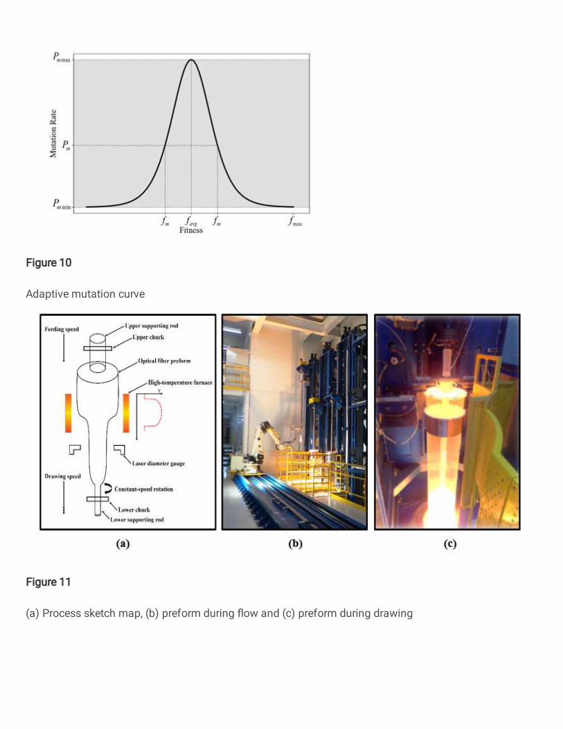
Figure 10

Adaptive mutation curve

Figure 11

(a) Process sketch map, (b) preform during �ow and (c) preform during drawing

Figure 12

Simulation modeling ideas

Figure 13

Physical-virtual production system interface

Figure 14

Field test results