1

A Demand Oriented Service Planning Process

Chi-Kang LEEDepartment of Transportation andCommunication ManagementNational Cheng Kung University1, University RoadTainan, 70101, TAIWANFax:+886-6-275 3882Email: cklee@mail.ncku.edu.tw

Wen-Jin HSIEHDepartment of Marketing and LogisticsManagementSouthern Taiwan Univ. of Technology1, Nan-Tai StreetYung Kang City, Tainan, TAIWANFax:+886-6-2422420Email:wjhsieh@mail.stut.edu.tw

ABSTRACTThe paper presents a service planning process of passenger railway for a regular

interval with variable train demand. The planning process consists of the estimation

of train demand, the design of service plan, and the construction of timetable. A train

demand model is to solve the service choice problem and estimate the demand for

each train service, given the detailed service information. A service design model is

to find a good service plan, in terms of service line, stopping pattern, and train

frequency, given the estimated train demand. A timetable construction model is to

find a good train diagram for the train movements over time and space, given an ideal

service plan. The proposed planning process explicitly takes into account of the

consistency among the three planning steps. A numerical example of Taiwan high-

speed rail shows the function and performance of the models. In the study, the train

demand model is formulated as a route choice problem on a service network with a

generalized cost function, and it is a nonlinear programming problem. The service

design model is a bi-level program, where the operator is the decision maker of the

upper problem, and the passenger is the decision maker of the lower level problem.

The timetable construction model is written as a mixed integer programming problem,

to fulfill the service plan, and solve any possible conflict among train movements.

Keywords: Passenger railway, Service design, timetable construction, Bi-level programmingI. INTRODUCTION

A sequential process is widely used in planning railway service. Firstly, in

demand analysis, passenger�s service choice behavior is considered to build a train

demand model, so as to estimate the passenger volume for each train service

2

[Nuzzolo, et al, 2000]. Timetable and other service characteristics are important

input. Secondly, service plan is designed to reach a high objective value of the

railway operator, e.g. profit or revenue, with the estimated train demand [Bussieck, et

al., 1997]. The level of service of train service, e.g. train frequency, is the output of

service design. Thirdly, an operational train diagram is developed, based on the ideal

service plan, to resolve any possible conflict between train movements on the railway

network [Odijk, 1996]. Passenger�s information of train service is clear only if

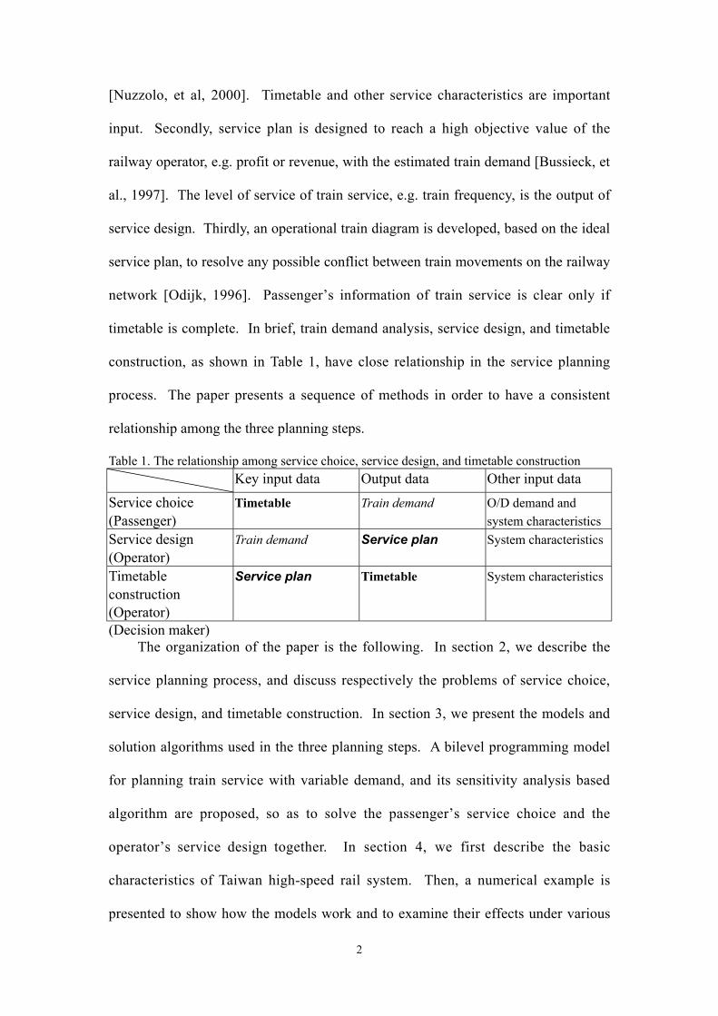
timetable is complete. In brief, train demand analysis, service design, and timetable

construction, as shown in Table 1, have close relationship in the service planning

process. The paper presents a sequence of methods in order to have a consistent

relationship among the three planning steps.

Table 1. The relationship among service choice, service design, and timetable constructionKey input data Output data Other input data

Service choice(Passenger)

Timetable Train demand O/D demand andsystem characteristics

Service design(Operator)

Train demand Service plan System characteristics

Timetableconstruction(Operator)

Service plan Timetable System characteristics

(Decision maker)The organization of the paper is the following. In section 2, we describe the

service planning process, and discuss respectively the problems of service choice,

service design, and timetable construction. In section 3, we present the models and

solution algorithms used in the three planning steps. A bilevel programming model

for planning train service with variable demand, and its sensitivity analysis based

algorithm are proposed, so as to solve the passenger�s service choice and the

operator�s service design together. In section 4, we first describe the basic

characteristics of Taiwan high-speed rail system. Then, a numerical example is

presented to show how the models work and to examine their effects under various

3

planning scenarios.

II. The Service Planning Process

2.1 Service Choice

The service choice problem is to describe the passenger�s choice behavior for

train service. In general, the information for passenger�s service choice includes

timetable, fare structure, access/egress transportation mode, etc [Nuzzolo, et al.,

2000]. In order to simplify the complexity of service planning process, we only

consider the choice of train service in the study, and ignore the choice of departure

time, the choice of access/egress mode, etc. The input of the service problem includes

basic characteristics of each train service, preference function of the passenger, and an

elastic O/D demand function. The output of the service problem is the passenger

volume for each train service and for each O/D pair. That is, not only the demand of

train service is a variable, but also the O/D demand is elastic to the quality of the

given service plan.

We assume the passenger is a cost minimizer, and his choice criterion or

preference is a linear generalized cost function, c(x, f); where IVT is in vehicle travel

time, OVT(f) is out of vehicle travel time, OPC is out of pocket cost, and CDC(x,f) is

crowding or discomfort condition; in which x is passenger volume in the train, and f is

train frequency in the regular interval.

C(x,f) = a0 + OPC + a1 IVTT + a2 OVTT(f) + a3 CDC(x,f);

Moreover, a1 and a2 are the time value of IVT and OVT respectively. IVT equals to the

sum of the train running time and dwell time. It is usually fixed for a specific railway

system. OVT equals to the sum of access time, waiting time, transfer time, and egress

time. It is dependent on train frequency f. OPC is the product of distance and fare

rate, and the fare rate is fixed for each train service. CDC is an index of crowing

condition, and it is defined as follows, where Q� is the practical capacity of the train.

])([ 'θω Q

xIVTCDC =

It is evident that CDC is a penalty associated with IVT. If the flow x equals to the

4

practical capacity Q�, CDC represents an increase of IVT by ω. The practical seating

capacity is dependent on train frequency f. If the train is very crowded, the load factor

is much bigger than 1 and the value of CDC is very big.

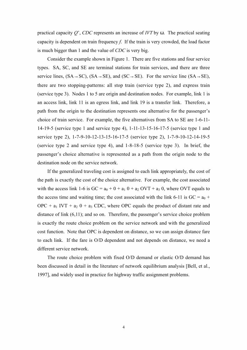
Consider the example shown in Figure 1. There are five stations and four service

types. SA, SC, and SE are terminal stations for train services, and there are three

service lines, (SA→SC), (SA→SE), and (SC→SE). For the service line (SA→SE),

there are two stopping-patterns: all stop train (service type 2), and express train

(service type 3). Nodes 1 to 5 are origin and destination nodes. For example, link 1 is

an access link, link 11 is an egress link, and link 19 is a transfer link. Therefore, a

path from the origin to the destination represents one alternative for the passenger�s

choice of train service. For example, the five alternatives from SA to SE are 1-6-11-

14-19-5 (service type 1 and service type 4), 1-11-13-15-16-17-5 (service type 1 and

service type 2), 1-7-9-10-12-13-15-16-17-5 (service type 2), 1-7-9-10-12-14-19-5

(service type 2 and service type 4), and 1-8-18-5 (service type 3). In brief, the

passenger�s choice alternative is represented as a path from the origin node to the

destination node on the service network.

If the generalized traveling cost is assigned to each link appropriately, the cost of

the path is exactly the cost of the choice alternative. For example, the cost associated

with the access link 1-6 is GC = a0 + 0 + a1 0 + a2 OVT + a3 0, where OVT equals to

the access time and waiting time; the cost associated with the link 6-11 is GC = a0 +

OPC + a1 IVT + a2 0 + a3 CDC, where OPC equals the product of distant rate and

distance of link (6,11); and so on. Therefore, the passenger�s service choice problem

is exactly the route choice problem on the service network and with the generalized

cost function. Note that OPC is dependent on distance, so we can assign distance fare

to each link. If the fare is O/D dependent and not depends on distance, we need a

different service network.

The route choice problem with fixed O/D demand or elastic O/D demand has

been discussed in detail in the literature of network equilibrium analysis [Bell, et al.,

1997], and widely used in practice for highway traffic assignment problems.

5

1

Service Type

2

3

4

5

SA

SB

SC

SD

SE

876

1411

191817

9

10

12

13

15

16

1

6

5

4

32

7

89

10

11

12

13

14

15

16

1817

19

20

2122

24

23

25 26 27

431 2

Figure 1: An Example Service Network

2.2 Service Design

Service design is one of the most important tasks in the strategic and tactical

planning for a railway operator, and it may include all variables in the marketing mix.

In the study, we only consider the design of service, i.e. the product strategy in the

marketing mix. The design of passenger train service is usually considered for the

regular interval, or a periodic timetable [Hooghiemstra, et al., 1996]. In a fixed

interval (e.g. in one hour), service decisions are selections of service line, stopping-

pattern, train length, and service frequency. In a rail network system, a line plan

6

determines the routes connecting two terminal stations, and it is the basis of a

timetable [Bussieck, et al., 1997]. For a service line, the main concern is selection of

stopping pattern, which specifies a set of stations where the train stops [Eisele, 1968].

A number of stop-patterns, such as all-stop, skip-stop, and zone-stop, have been

identified and extensively studied, primarily for the many-to-one problem on a

commuter rail line [Eisele, 1968; Sone, 1992]. For an inter-city rail line, research

results show that there is no the best stopping-pattern [Chang, et al, 2000]. Moreover,

in a rail line, the decision of service line is simple, and it can be considered with

stopping-pattern together. In this study, the output of the service design problem is a

set of service types (service line and stopping-pattern) and their associated service

frequency.

Some studies have shown the advantages in dealing with both operator�s and

passenger�s objectives in the service planning for a transportation operator [Fu, et al.,

1994]. In general, passenger is shortsighted on his choice, and will not consider the

reaction of other passengers or the railway operator. On the contrary, the railway

operator usually makes his/her service plan with consideration of the passenger�s

possible reactions. In order to reflect the asymmetric information relationship

between the operator and the passenger, it is appropriate to solve the passenger�s

service choice and the operator�s service design together as a Stackelberg game.

Bilevel programming describes a Stackelberg game, where two decision-makers, each

with one�s objective, act and react in a non-cooperative manner [Bard, 1998]. In this

study, the operator�s design model for planning service type (s) and train frequency (f)

is the upper-level problem, and a demand model for passenger�s choice of train

service (x, t) is the lower level problem. The bilevel program is written as follows,

and it is used to solve the consistency between service choice and service design.

7

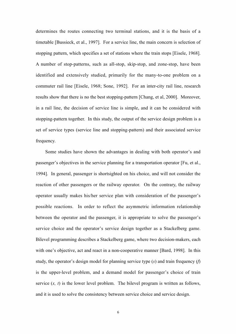
Maximize: Operator�s objective (s, f, x, t)(s, f)s.t. Fleet size

Line capacity

Seating capacity

etc.

Minimize: Passenger�s objective (x, t)

(x, t)s.t. A given choice set (or service plan)

etc.

2.3 Timetable Construction

A service plan is operational only if we have its associated timetable or train

diagram. In the service choice problem and service design problem discussed above,

we do not consider time-dependent choice behavior and service plan, e.g. the

departure time of passenger or the departure time of train. Hence, we need a

timetable construction model to take into account of the train movements over time

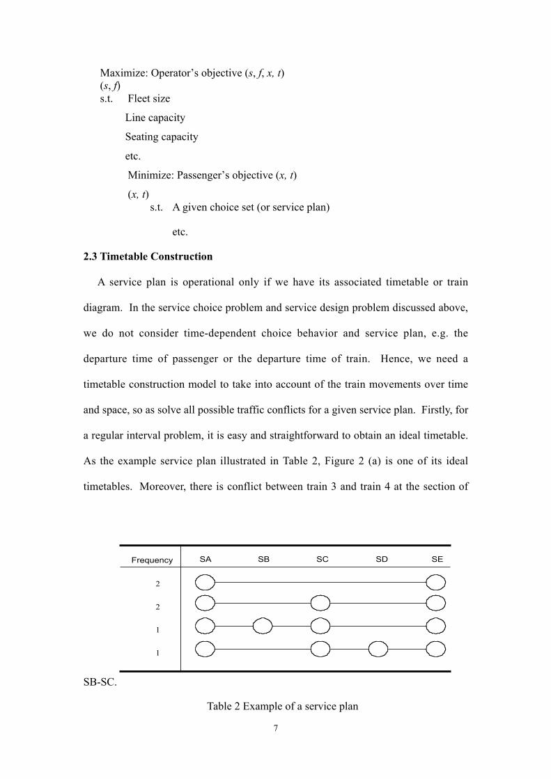
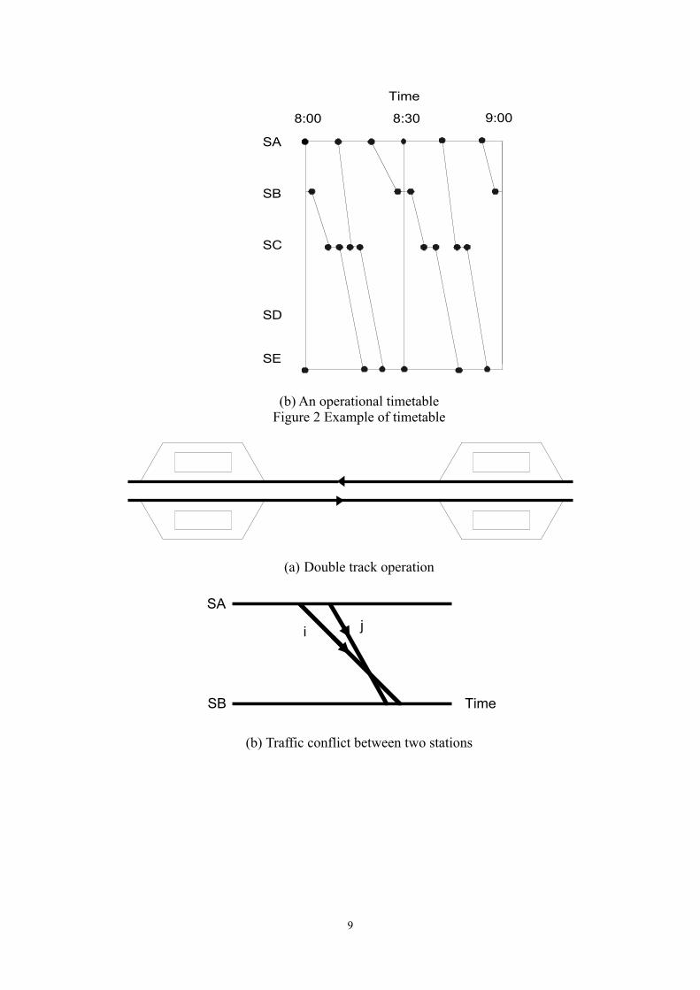
and space, so as solve all possible traffic conflicts for a given service plan. Firstly, for

a regular interval problem, it is easy and straightforward to obtain an ideal timetable.

As the example service plan illustrated in Table 2, Figure 2 (a) is one of its ideal

timetables. Moreover, there is conflict between train 3 and train 4 at the section of

SB-SC.

Table 2 Example of a service plan

SA SCSB SESD

2

1

1

2

Frequency

8

Given an ideal scheduled arrival and departure times at scheduled stop stations for

each train, a timetable construction model is to find the operation plan to move the

trains from their origins to final destinations that is consistent with physical and

operational constraints [Jovanovic, et al., 1991]. For the operation of double track

with an island platform at each station, as the example shown in Figure 3(a), we

illustrate some possible traffic conflicts in Figure 3(b) and 3(c). The primary

challenge in solving timetable construction problem is to determine the appropriate

locations for each conflicting train to overtake and/or meet another train. For the

example shown in Figure 2(a), we can decrease the departure time of train 3 a little, so

as to have the operational timetable shown in Figure 2(b).

9:00

SA

SB

SC

SD

SE

8:30Time

8:00

1 2 3 4 5 6

(a) An ideal timetable

9

9:00

SA

SB

SC

SD

SE

8:00 8:30

Time

(b) An operational timetableFigure 2 Example of timetable

(a) Double track operation

SA

SB Time

i j

(b) Traffic conflict between two stations

10

SB

Time

i lk

ki

(c) Traffic conflict at station

Figure 3 Example of traffic conflict

In the service planning process, the final timetable obtained in the last step should

have all basic characteristics of the service information used in the first step of service

choice problem, or in the bilevel service design problem. Therefore, the deviation

between the service plan and its associated timetable is minimized in the timetable

construction problem. That is, we change the departure time, dwell time, or running

time in the ideal timetable as small as possible.

III The Service Planning Models

3.1 A Train Demand Model with Elastic O/D Demand

3.1.1 The train demand model

Assuming cost minimizing behavior and independent choice for each road user,

Nash equilibrium flow pattern is commonly used for the route choice problem. The

user equilibrium network model deals with the interaction among the road users� route

choices. For a rail line, one passenger�s choice is dependent on other passengers�

choices, when the seating capacity or crowding effect is considered. Because the cost

function used in this study is dependent on flow variable x, the route choice problem

is then written as a nonlinear programming problem.

11

∑∫∑∫ −−),(

)()(minji

t

ijl

x

a

ijl

dxxddxxc0

1

0 (1)

s.t. xhA =⋅ (2) thB =⋅ (3) 0≥h (4)

Where a is link index, x is link flow vector, (i,j) is origin destination index, d(.) is

demand function, h is path flow vector, t is the origin and destination (O/D) matrix, A

is the link-path incidence matrix, and B is the O/D-path incidence matrix. The model

characteristics and solution algorithm have been widely discussed in detail in the

literature [Bell, 1997].

The Lagrangian of the nonlinear programming model is

hkh)Bt(ztAhxfkz,th,L TT ⋅+⋅−+== ),(),( (5)

f(.) is the objective function (1), z is the dual variable associated with O/D demand

constraint (3), and k is the Lagrange multiplier associated with constraint (4). At

optimality, the first order condition for path flow and origin/destination demand are

equations (6) and (7) respectively.

0),(),( =+⋅−=∇=∇ kzBtAhxfkz,th,L Thh (6)

0),(),( =+=∇=∇ ztAhxfkz,th,L tt (7)

By the objective function (1) and the definitional constrain (2), we obtain equation (8)

for path cost g and link cost c. In addition, link cost is further written as sum of flow

independent cost and flow dependent cost, )()( 10 xx ccc += .

gxccAxcAthf TTh =+⋅=⋅=∇ ))(()(),( 10

(8)

At optimality, we have equation (9) for the positive path flow by equation (6). The

path cost for used path equals to the dual variable z, which is only dependent on

origin/destination. Moreover, it is evident that the path cost of unused path is greater

than or equal to the dual variable z.

zBgthf Th ⋅==∇ ),( (9)

12

Moreover, we get the optimal origin/destination traveling cost (10) or the optimal

origin/destination demand (11), by the first order condition (7).

ztd =− )(1 (10)

tzd =)( (11)

3.1.2 Sensitivity Analysis of the Model

Given a service plan in terms of train frequency (f) for each service type, the

train demand model estimates equilibrium passenger volume (x) and origin

destination demand (T). The sensitivity relationship between the model input (f) and

model outputs (x, T) is written as (12) and (13).

fc

cz

zx

fx

xf ∆∆

∆∆

∆∆

∆∆ ⋅⋅==∇ (12)

fc

cz

zT

fT

Tf ∆∆

∆∆

∆∆

∆∆ ⋅⋅==∇ (13)

The relationship between train frequency (f) and the generalized cost (c) is clear, so

we can compute fc ∆∆ / accordingly. In the following, we will discuss the derivation

of zT ∆∆ / , zx ∆∆ / , and cz ∆∆ / .

First, by the demand function (11), we get zT ∆∆ / = )(zd∇ at optimal. Secondly,

the total derivative of zABxccAA TT =+ ))(( 10 is written as equation (14), by

equations (8) and (9).

zABxxcAA TT ∆=∆∇ )(1 (14)

If the inverse of ATA exists or the rank of ATA equals to the number of used path

[Searle, 1971], we obtain zx ∆∆ / as equation (15).

TT ABxcAAzx 1

1 ))((Ä

−∇=∆(15)

Thirdly, by equations (8) and (9), we obtain the total derivative of the path cost g,

with respect to flow variable x and dual variable z, as equation (16).

13

zBxxAzzg

xxg

g TT ∆+∆∇=∆∆∆+∆

∆∆=∆ )(1c (16)

By the equation (8) of path cost and link cost, cAg T∆=∆ . If the inverse of ATA

exists or the rank of ATA equals to the number of used path, it follows equation (17).

zABAAxxcc TT ∆+∆∇=∆ −11 )()( (17)

Moreover, by constrain (3) and equation (11), we have the total derivative of origin/destination

demand as equation (18),

zzdxBG

zzdxAABAzzdhBt TT

∆∇+∆=∆∇+∆=∆∇+∆=∆ −

)(

)()()( 1

(18)

where, 1)( −= TT AAAG .

By the equations (17) and (18), we get equation (19).

∆∆

∇

∇=

∆∆ −

z

x

zdBG

ABAAxc

t

c TT

)(

)()( 11 (19)

By the inverse operation of the partitioned matrix, it follows that

∆∆

=

∆∆

t

c

JJ

JJ

z

x

2221

1211 (20)

where, )xcBGF)FxcBGzTF((IxcJ 111111

−−−−− ∇∇−∇−−∇= ))()(()))()(()(())(( 11

11

111 )))()(()(())(( −−− ∇−∇∇= FxcBGzTFxcJ 11

12

1121 xBGFxBGzTJ −−− ∇∇−∇−= ))()(()))()(()(( 1

11 cc

1122 FxBGzTJ −−∇−∇= )))()(()(( 1c

TT ABAAF 1)( −=

Therefore, we find =∆∆ cz / J22.

3.2 A Bilevel Service Design Model

3.2.1 The service design model

14

The objective of the design problem is usually to minimize the total operating cost,

or to maximize the profit. The model for maximizing profit is written as follows.

Max

⋅⋅+⋅⋅+⋅−⋅ ∑ ∑∑

s sssss

lll sRCfDCNCxP 321 (21)

s.t. a

sss RNfR ⋅≤⋅∑ (22)

bsSs

s

bsSs

s

Ssbss

SsbssSs

bss

f

f

f

ff

γ

γϕ

γ

γϕ

γ

⋅

⋅⋅+

⋅

⋅⋅

≤⋅

∑∑

∑∑∑

∈

∈

∈

∈∈

22

11

60 , ∀ b (23)

lsls xfQ ε⋅≥⋅ , ∀ l,s (24)

∑ ≥⋅s

sis s 1α , ∀ i (25)

∑ ≥⋅s

sjs s 1β , ∀ j (26)

ss sMf ⋅≤ , ∀ ,s (27)

+∈ Zfs , { }10,ss ∈ (28)

),( min TAhxf = (1) s.t.

ThB =⋅ (3)

0≥h (4)

Notation:

Pl : Price or fare for link l.

C1: fixed overhead cost ($ / train).

N: fleet size (trains).

C2: distance dependent variable cost ($ / train-km).

Ds: running distance of service type s (km).

C3: time dependent variable cost ($ / train-minute).

Rs: running time of service type s (minute).

Ra: average available running time for the planning interval (minute).

ϕ1, ϕ2: parameters for speed group 1 and group 2.

γbs: a zero-one index. It is one if the section b is a part of the service s.

15

S: the set of service type.

S1: the set of service type with high average speed.

S2: the set of service type with relative low average speed.

Q: the seating capacity of a train.

εls: a zero-one index. It is one if the link l is a part of the service s.

α is: a zero-one index. It is one if the service s coves the origin i.

βjs: a zero-one index. It is one if the service s covers the destination j.

M: a big positive number.

As the example illustrated in Figure1, a service type represents a combination of

service line and stop pattern. S denotes the set of service type. The service design

model is to find the optimal subset of service types, and the frequency for each service

type. A zero-one variable ss represents selection of service type s, and an integer

variable fs represents train frequency of service type s. By the constraint (27), it is

evident that fs > o only if ss =1.

Profit is the dif ference between revenue and operating cost. Assu me the fare rate

is a constant ($/km) and it is not O/D dependent, the price for each link Pl is a

constant, and the revenue can be computed by link. For each service type, the

operating distance Ds, and operating time Ts are given, because the running and dwell

times are fixed for a specific system. Moreover, the following cost parameters are

given: fixed overhead cost C1, distance dependent operating cost C2, and time

dependent variable cost C3. With the parameters of price, cost, and service

characteristics, the profit function is written as (21).

The inequality (22) is fleet size constraint for the regular interval. The inequality

(23) is line capacity constrain used in practice. A section of rail line is the place

between two consecutive stations. The line capacity is dependent on the speed

difference among trains. In constrain (23), it is assumed that there are two speed

16

groups. In the service planning stage, the seating capacity constraint (24) provides

enough seats for passengers at each service link. Hence, it is not necessary to have a

capacity constraint in the passenger�s choice problem. Moreover, constraint (25) and

constraint (26) make sure that there is at least one service type for each origin and

each destination.

The passenger�s choice model is one constrain of the service design model. The

service type variable s, in the upper level problem, will decide the structure of service

network for the lower level problem. As described in section 2.4, the frequency

variable f, in the upper level problem, has direct effect on the link cost, and indirect

effect on link passenger volume and origin/destination demand, in the lower level

problem. Moreover, the decision variable x in the lower level problem is a variable of

the objective function (21) and the seating capacity constraint (24) in the upper level

problem.

3.2.2 Solution Algorithm

There are several approaches to solve a bilevel programming problem [Bard,

1998]. For an equilibrium network design problem, sensitivity analysis based

methods are usually suggested for a Stackelberg solution [Bell, 1997; Yang, et al.,

1998]. Several sensitivity analysis methods for the equilibrium network problem have

been studied [Tobin, et al, 1988; Cho, et al., 2000]. The iterative sensitivity algorithm

procedure used in the study is listed in the following.

Step 0 (Initialization)

Set k=0, and find an initial solution f k and sk with the set of service type S.

Step 1 (Lower level problem)

Solve the passenger�s choice problem for x,k and tk, given f k and sk. The

nonlinear programming problem is solved by the Frank-Wolfe algorithm or

17

the method of successive averages.

Step 2 (Sensitivity analysis)

Compute the sensitivity of train frequency f to link flow x as kf x∇ and

kf t∇ .

Step 3 (Linear reaction function)

Set the linear reaction functions, )( 11 kkkf

kk ffxxx −∇+= ++ and

)( 11 kkkf

kk ffttt −∇+= ++ .

Step 4 (Upper level problem)

Solve the upper level problem for f k+1 given the linear reaction functions.

The upper level problem is solved by the branch and bound method.

Step 5 (Convergence test)

If it is converged, stop; otherwise, k=k+1 and go to step 1.

3.3 A Timetable Construction Model

The objective of the timetable construction model is to minimize the total

deviation of departure time, dwell time, and running time. The model is listed as

follows.

)()( Min mi

Ii Ii Dm

mi

Gi

Gi leZ µε∑ ∑∑

∈ ∈ ∈

+++= (29)

subject to_

(1) schedule constraints_

Iil ed Oi

Oi

Oi

Oi ∈∀+−=δ (30)

imi

mi

mi

mi QmIida ∈∈∀++=+ , 1 µτ (31)

imi

mi

mi

mi

mi QmIiad ∈∈∀+−+= , εσδ (32)

(2)train following and overtaking constraints_

kimik

mik

mi

mk QQmIkibdd ∩∈∈∀−−+≥ , , )1(ψξ (33)

kimik

m

ik

mi

mk QQmIkibdd ∩∈∈∀−+≥ , , ψξ (34)

kimik

m

ik

mi

mk QQmIkibaa ∩∈∈∀−−+≥ +++ , , )1(

!11 ψη (35)

kimik

m

ik

mi

mk QQmIkibaa ∩∈∈∀−+≥ +++ , ,

111 ψη (36)

kimik

mik QQmkiIkibb ∩∈<∈∀≤ − , ,, 1

(37)

18

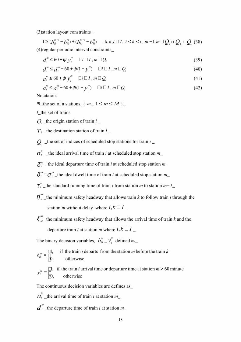
(3)station layout constraints_

QQQbbbb lki

mkl

mkl

mik

mik mmlkiIlki ∩∩∈−<<∈∀−+−≥ −− ,1 , ,,, )()(1 11 (38)

(4)regular periodic interval constraints_

i

m

i

mi QmIiyd ∈∈∀+≤ , 60 ψ (39)

i

m

i

mi

mi QmIiydd ∈∈∀−+−≤ , )1(60 ψ (40)

i

m

i

mi QmIiya ∈∈∀+≤ , 60 ψ (41)

i

m

i

mi

mi QmIiyaa ∈∈∀−+−≤ , )1(60 ψ (42)

Notataion:

m_the set of a stations, { m _ Mm ≤≤1 }_

I_the set of trains

Oi _the origin station of train i _

T i _the destination station of train i _

Qi _the set of indices of scheduled stop stations for train i _

σ mi _the ideal arrival time of train i at scheduled stop station m_

δ mi _the ideal departure time of train i at scheduled stop station m_

σδ mi

mi − _the ideal dwell time of train i at scheduled stop station m_

τ mi _the standard running time of train i from station m to station m+1_

η m

ik _the minimum safety headway that allows train k to follow train i through the

station m without delay_where Iki ∈, _

ξ m

ik _the minimum safety headway that allows the arrival time of train k and the

departure train i at station m where Iki ∈, _

The binary decision variables, bmik _ y

m

i defined as_

= otherwise ,0

train thebefore station thefrom departs train theif ,1 kmibm

ik

>

= otherwise ,0

minute 60 station at timedepartureor timearrival train theif ,1 miym

i

The continuous decision variables are defines as_

am

i _the arrival time of train i at station m_

dm

i _the departure time of train i at station m_

19

lG

i_the pre-departure time of train i at origin station Oi _

eG

i _the delay departure time of train i at origin station Oi _

em

i_the schedule delay of train i at station m_

miε = the delay dwell time of train i at station m_

miµ = the delay standard running time of train i from station m to station m+1_

ψ =a large positive number.

Schedule constrains are equations (30), (31), and (32). They are definitional

constrains and define the basic relations among these schedule variables. Equations

(33) to (37) deal with train following and overtaking constrains. They are used to

solve the traffic conflict illustrated in Figure 3(a). Station track layout constrain is

equation (38). It is used to solve the traffic conflict shown in Figure 3(b). Finally,

equations (39) to (42) deal with the problem of regular periodic interval.

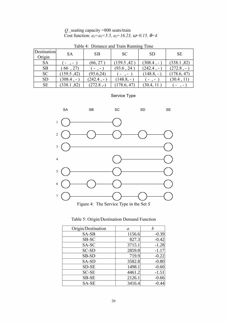
IIII. Numerical Example

4.1 Data

The models developed in the study were motivated by the high-speed rail project

in Taiwan [Lin, 1995]. The HSR system is about 340-kilometer long, and located

along the western corridor of Taiwan. It connects three metropolitans, and 7 cites of

medium size. In the paper, we use a test example of 5 stations and 7 service types to

demonstrate the effectiveness of the model. Tables 3 and 4, and Figure 4 show the

relevant data inputted to the model. Table 3 is the input parameters of the bilevel

model. In Table 4, the figures in parenthesis are respectively the distance (km) and

train running time (minute). The train running time is the direct running without any

intermediate stop. The origin/destination demand function, ijij cbat ⋅−= , is

estimated using the forecasted demand data for 8 a.m. to 9 a.m. in 2003. The

parameter used in the demand model is listed in Table 5.

Table 3: Input Parameters of the Model

Fare rate_3.54 (NT$/km)1C _fixed overhead cost in the regular interval = 4551(NT$/train)2C _operating distance dependent variable cost = 91.4536(NT$/train-

km)

3C _operating time dependent variable cost =825.5 (NT$/train-hour)S _the set of feasible service types { }7,6,5,4,3,2,1 sssssssS =N _fleet size =30 trains

20

Q _seating capacity =800 seats/trainCost function: a1=a3=5.5, a2=16.23, ω=0.15, θ=4.

Table 4: Distance and Train Running TimeDestination

OriginSA SB SC SD SE

SA ( - , - ) (66, 27 ) (159.5 ,42 ) (308.4 , - ) (338.1 ,82)SB ( 66 , 27) ( - , - ) (93.6 , 24 ) (242.4 , - ) (272.8 , - )SC (159.5 ,42) (93.6,24) ( - , - ) (148.8, - ) (178.6, 47)SD (308.4 , - ) (242.4 , - ) (148.8, - ) ( - , - ) (30.4 , 11)SE (338.1 ,82) (272.8 ,-) (178.6, 47) (30.4, 11 ) ( - , - )

1

6

5

4

3

2

Service Type

7

SA SCSB SESD

Figure 4: The Service Type in the Set S

Table 5: Origin/Destination Demand Function

Origin/Destination a bSA-SB 1156.6 -0.39SB-SC 827.3 -0.42SA-SC 3715.1 -1.28SC-SD 2859.8 -1.17SB-SD 719.9 -0.22SA-SD 3582.8 -0.80SD-SE 1498.1 -0.60SC-SE 4461.2 -1.51SB-SE 2126.1 -0.66SA-SE 3416.4 -0.44

21

4.2 Testing Results

The major findings of the study are stated in the following.

1. Service Plan

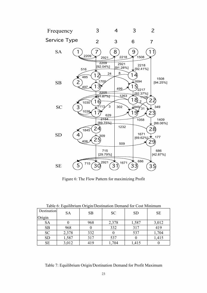
The optimal service plan obtained by the model is illustrated in Figures 5 for profit

maximum, or in Figure 6 for cost minimum. The number associated with each link is

passenger volume or passenger trips, and the number in parenthesis is load factor. For

both profit and cost objectives, the same service types are selected. They are service

type 2 of all-stop train, service type 3 of express train, service types 6 and 7 of limited

express train. The total train frequency is 12-train per hour for profit maximum, and

11-train per hour for cost minimum. There is one more all-stop train for profit

maximum than cost minimum.

2. Equilibrium Flow Pattern

As the equilibrium origin/destination demand shown in Table 6 and Table 7,

maximum profit operation approaches a high demand value and cost minimum

operation approaches a low demand value. The passenger volume of each train

service is shown in Figure 5 and Figure 6. The number of passengers of all-stop train

for profit maximum is higher than that for cost minimum. However, the load factor

patterns illustrated in Figure 5 and Figure 6 are not much different, partly because the

train frequency for cost minimum is one train few.

3. The Sensitivity of Train Frequency

In the case of minimizing total operating cost, the change of passenger flow in

response to an increase of the frequency of each is shown in Table 8. An increase of

direct express train of service type 3 from SA to SE results in an increase of 248

passengers, and a decrease of the passenger flow for other service types, e.g. a

decrease of 147 trips for service type 7. Hence, the sensitivity of train frequency to

the passenger flow pattern is evident. The sensitivity results of train frequency are not

only essential for solving the bi-level mathematical programming model, but also

useful in timetable construction process. When we extend a regular peak hour

timetable to be one-day timetable, the sensitivity results of stop pattern and train

frequency are used for modifying the timetable for off-peak periods. In addition,

many types of sensitivity results for service characteristics, e.g. sensitivity of fare

level and fare structure, can be computed for detail and practical discussion.

22

1

2

3

4

5

987

3330

12

19

31

11

23

29

35

1469[91.81%]

623

1315[82.18%]

95

803[50.18%]

22

28

1457 2865 2154 1469

477

5062242

[93.41%]1189

102

665886

690

708707

2078

1220

8032865804

953

1457[91.06%]

2154[89.75%]

2946[92.06%]

1469[91.81%]

723

104248

644

1319[82.43%]

2078[86.58%]

1221

97

804[50.25%]

1513

16

17

18

24

25

141013491

1667

562

798

9

2

Frequency

2 3 76Service Type

2 4 3 2

SA

SB

SC

SD

SE

Figure 5: The Flow Pattern for Minimizing Total Operating Cost

23

1

Frequency

2

3

4

5

SA

SB

SC

SD

SE

987

3330

12

2 3

19

31

7

11

23

29

35

1508[94.25%]

349

1409[88.06%]

177

686[42.87%]

22

28

2209 2921 2218 1508

516

4972217

[92.37%]1263

302

1038629

1058

509406

1671

1232

6862921715

1700

2209[92.04%] 2218

[92.41%]

2921[91.28%]

2205[91.87%]

1030

949 311113

2154[89.75%]

1671[69.62%]

1845

309

715[29.79%]

1513

16

17

18

24

25

14824485

1694

499

1128

6

3

2

Service Type

3 4 3 2

Figure 6: The Flow Pattern for maximizing Profit

Table 6: Equilibrium Origin/Destination Demand for Cost MinimumDestination

OriginSA SB SC SD SE

SA 0 968 2,378 1,587 3,012SB 968 0 332 317 419SC 2,378 332 0 537 1,704SD 1,587 317 537 0 1,415SE 3,012 419 1,704 1,415 0

Table 7: Equilibrium Origin/Destination Demand for Profit Maximum

24

Destination

OriginSA SB SC SD SE

SA 0 1001 2,978 1,645 3,232SB 1001 0 443 254 299SC 2,978 443 0 1,178 1,547SD 1,645 254 1,178 0 915SE 3,232 299 1,547 915 0

Table 8: Sensitivity of Train Frequency for Cost MinimumFrequencyPassenger

Flow S1 S2 S3 S4 S5 S6 S7SA_SE -51 -27 248 -27 -71 -32 -64SA_SC 154 -56 -147 95 135 -57 137SC_SE 88 -51 -72 131 134 107 -48SA_SB -103 83 -101 -73 -64 89 -73SB_SC -103 83 -101 -73 -64 89 -73SC_SD -37 78 -176 -104 -63 -75 112SD_SE -37 78 -176 -104 -63 -75 112

4. The sensitivity of O/D demand

In the case of maximizing profit, the change of passenger flow in response to one trip

increase of an O/D demand is shown in Table 9. For example, 71.3% of the increased

trip from SA to SE will use service type 3 from SA to SE directly. 18.2% will use

service type 7 from SA to SC. Besides, many types of sensitivity analysis for demand

characteristics, e.g. sensitivity of O/D demand pattern, can be computed for detail and

practical discussion.

Table 9: Sensitivity of O/D DemandThe Sensitivity of O/D Demand

Passenger FlowChange Rate SA/SE SB/SE SA/SC SC/SE

SA_SE 0.713 0 0 0SA_SC 0.182 0 0.658 0SC_SE 0.18 0.587 0 0.724SA_SB 0.105 0 0.342 0SB_SC 0.105 1 0.342 0SC_SD 0.142 0.413 0 0.276SD_SE 0.142 0.354 0 0.276

5. Solution Algorithm for the bilevel program

Although the interface between the upper-level and the lower-level problems, such as

the service network construction for the lower-level problem and the calculation of

the sensitivity result for the upper-level problem, is complex and difficult; the

convergence of the iterative sensitivity algorithm for solving the bilevel program with

25

the numerical example is efficient and acceptable. As the result shown in Figure 7,

the method does not get a descent or ascent direction at each iteration, however, it

converges to the same optimal solution with three different initial solutions. Hence,

we can obtain the optimal solution within acceptable time consumption.

3700000

3750000

3800000

3850000

3900000

3950000

4000000

4050000

4100000

1 4 7 10 13 16 19 22 25 28 31 34 37 40 43 46 49Iterations

Prof

it($)

Init. Sol.1

Init. Sol.2

Init. Sol.3

Figure 7: The Convergence of the Sensitivity-based Solution Algorithm6. Timetable

Given a service plan, we can construct several ideal timetables with consideration of

the time slot allocation for each train in the regular interval. For each ideal timetable,

we obtain its associated operational timetable by using the timetable construction

model. For example, Figure 8 shows the case of minimum cost problem and Figure 9

illustrates the case of maximum profit. It is evident that the circled traffic conflicts in

Figure 8(a) or Figure 9(a) are solved only by small change of schedule variables.

Therefore, the ideal timetable and the operational timetable have similar service

characteristics, such as the headway of a service type, the in-vehicle travel time, and

so on.

26

9:00

SA

SB

SC

SD

SE

8:00 8:30

Time

(a) The ideal timetable

9:00

SA

SB

SC

SD

SE

8:00 8:30

Time

(b) The optional timetable

Figure 8: Timetable of Minimum Cost Problem

27

9:00

SA

SB

SC

SD

SE

8:00 8:30

Time

(a) The ideal timetable

9:00

SA

SB

SC

SD

SE

8:00 8:30

Time

(b) The optional timetableFigure 9: Timetable of Maximum Profit Problem

IV. Concluding Remarks

In order to have a consistent relationship, we study the following three steps in

28

the railway planning together: service choice, service design, and timetable

construction. From the demand side, we consider the passenger�s service choice and

elastic O/D demand explicitly in the planning process. From the supply side, we build

the operator�s service design model with consideration of the passenger�s responsive

behavior. From the operation point of view, we have a timetable construction model

to fulfill the service plan by solving possible traffic conflicts.

In this study, service choice is a nonlinear programming problem, and it is the

lower-level problem in the service design structure. The service design model is an

integer linear programming problem, and it is the upper-level problem in the service

design structure. The timetable construction model is a mixed integer programming

problem. The developed models are tested with the case of Taiwan HSR, and obtain

promising planning results.

The paper is only an initial step for the railway planning with variable demand.

Various further studies can be done so as to clarify the relationship between the

operator�s marketing variables, e.g. price level and price structure, and the

passenger�s choice behavior, e.g. stochastic service choice. Moreover, the three

planning steps can be integrated into one model, if we add the time dimension into the

bilevel program for service choice and service design.

Acknowledgements: The authors are grateful to the financial support by the NationalScience Council, Taiwan, R.O.C. under the contract of NSC89-2211-E-006-046.

Reference

Bard, J. F. (1998) Practical Bilevel Optimization- Algorithms and Applications. KluwerAcademic Publishers.

Bell, M. G. H. and Y. Iida.(1997) Transportation Network Analysis. John Wiley & Sons,Inc., U.S.A.

Bussieck, M.R., P. Kreuzer and U. T. Zimmerman.(1997) Optimal Lines for Railway Systems.European Journal of Operational Research, Vol.96, pp.54-63.

Chang, Y-H, Yeh, C-H, and Shen, C-C.(2000) A Multiobjective Model for Passenger TrainServices Planning: Application to Taiwan�s High-speed Rail Line. Transportation Research,Vol.34B, pp.91-106.

Cho, H-J, T. E. Smith, and T. L. Friesz.(2000) A Reduction Method for Local SensitivityAnalyses of Network Equilibrium Arc Flows. Transportation Research, Vol. 34B, pp.31-51.

Eisele, D. O.(1968) Application of Zone Theory to a Suburban Rail Transit Network. TrafficQuarterly, Vol. 22, pp.49-67.

Fu, Z., and M. Wright.(1994) Train Plan Model for British Rail Freight Services through the

29

Channel Tunnel. Journal of the Operational Research Society, Vol. 45, pp.384-391.

Hooghiemstra, J. S.(1996) Design of Regular Interval Timetables for Strategic and TacticalRailway Planning. In Computers in Railway V, Vol. 1, Edited by. J. Allan, C. A. pp.393-402,

Jovanovic, D. and Harker, P.T. (1991) Tactical scheduling of rail operations: the SCANIsystem. Transportation Science Vol. 25, pp.46-64.

Lin, C-Y. The high-speed rail project and its privatization in Taiwan. Rail International,1995. pp.175-179.

Nuzzolo, A., Crisalli, U., and Gungemi, F.(2000) A Behavioral Choice Model for theEvaluation of Railway Supply and Pricing Policies. Transportation Research, Vol. 34A, pp.395-404.

Odijk, M.A. (1996) A constraint generation algorithm for the construction of periodic railwaytimetables. Transportation Research, Vol. 30B, pp.455-464.

Searle, S. R., (1971), Linear Models. New York: Wiley.

Sone, S.(1992) Novel Train Stopping Patterns for High-frequency, High-speed TrainScheduling. Computers in Railways III- Volume 2 eds. T.K.S. Murthy, J. Allan, R.J. Hill, G.Sciutto, S. Sone, Computational Mechanics Publications, U.K, pp.107-118.

Tobin, R. L. and Friesz, T. L.(1988) Sensitivity Analysis for Equilibrium Flow.Transporation Science, Vol. 22, pp.242-250.

Yang, H., and Bell, G. H.(1998) Models and Algorithms for Road Network Design: a Reviewand Some Developments. Transport Reviews, Vol. 18, pp.257-278.