A Delay Damage Model Selection Algorithm for NARXNeural NetworksTsungnan Lin 1;2�,C. Lee Giles 1;3, Bill G. Horne 1, S.Y. Kung 21 NEC Research Institute, 4 Independence Way, Princeton, NJ 085402 Department of Electrical Engineering, Princeton University, Princeton, NJ 085403 UMIACS, University of Maryland, College Park, MD 20742U. of Maryland Technical Report CS-TR-3707 and UMIACS-TR-96-77AbstractRecurrent neural networks have become popular models for system identi�cation and timeseries prediction. NARX (Nonlinear AutoRegressive models with eXogenous inputs) neuralnetwork models are a popular subclass of recurrent networks and have been used in manyapplications. Though embedded memory can be found in all recurrent network models, it isparticularly prominent in NARX models.We show that using intelligent memory order selection through pruning and good initialheuristics signi�cantly improves the generalization and predictive performance of these nonlinearsystems on problems as diverse as grammatical inference and time series prediction.Keywords: Recurrent neural networks, tapped{delay lines, long{term dependencies,time series, automata, memory, temporal sequences, gradient descent training, latching,NARX networks, auto{regressive, pruning, embedding theory.�Current address: Epson Palo Alto Laboratory, 3145 Porter Drive, Suite 104, Palo Alto, CA 943041

1 IntroductionNARX (Nonlinear AutoRegressive models with eXogenous inputs) recurrent neural architectures [6,41], as opposed to other recurrent neural models, have limited feedback architectures which come onlyfrom the output neuron instead of from hidden neurons. It has been shown that in theory one canuse NARX networks, rather than conventional recurrent networks, without any computational lossand that they are at least equivalent to Turing machines [53]. Not only are NARX neural networkscomputationally powerful in theory, but they have several advantages in practice. For example, ithas been reported that gradient-descent learning can be more e�ective in NARX networks than inother recurrent architectures with \hidden states" [25].Part of the reason can be attributed to the embedded memory of NARX networks. This em-bedded memory will appear as jump-ahead connections which provide shorter paths for propagatinggradient information more e�ciently when the networks are unfolded in time to backpropagatethe error signal and thus reduce the network's sensitivity to the problem of long-term dependen-cies [34, 36].Not only can the embedded memory reduce the sensitivity to long-term dependencies, but it alsoplays an important role in learning capability and generalization performance [35]. In particular,forecasting performance could be seriously de�cient if a model's memory architecture is either inad-equate or unnecessarily large. Therefore, choosing the appropriate memory architectures for a giventask is a critical issue in NARX networks.The problem of memory-order selection is analogous to that of choosing an optimal subset ofregressors variables in statistical model building. In optimal subset selection, it is desired that themodel includes as many regressors as possible so that the information content in these regressorswill in uence the predicted value of the dependent variable; on the other hand, it is also desiredthat the model includes as few regressors as possible because the variance of the model's predictionsincreases along with the increasing number of regressors [39].According to the embedding theorem [45, 51, 57], the memory orders need to be large enough in2

order to provide a su�cient embedding. The problem of choosing the proper memory architecturecorresponds to give a good representation of input data. A good representation can make usefulinformation explicit and easy to extract. Two di�erent representations can be equivalent in termsof expressive power, but may di�er dramatically in the e�ciency or e�ectiveness of problem-solving.When there is no prior knowledge about the model of the underling process, traditional statisticaltests can be used, for example, Akaike information criterion (AIC) [1] and the minimumdescriptionlength principle (MDL) [50]. Such models are judged on their \goodness-of-�t", which is a functionof the likelihood of the data given the hypothesized model and its associated degrees of freedom.Fogel [16] applied the modi�cation of AIC to select a \best" network. However, the AIC method iscomplex and can be troubled by imprecision [52, 23].Evolutionary Programming [2, 18] is another search mechanism. This algorithm operates on apopulation of models. O�spring models are created by randomly mutating parents models. Compe-tition between o�spring models for survival are judged according to the �tness function. Fogel [17]used evolutionary programming for order selections of linear models in a time series of ocean acousticdata. But the algorithm can be computationally expensive when the underling process is complexand nonlinear.Alternatively, an adaptive algorithm which treats the delay operators as ordinary adjustableparameters can be a useful technique. This algorithm iteratively determines the memory of a modelbased on the gradient information. Originally proposed by Etter, it was used as a \adaptive delay�lter", which included variable delays taps as well as variable gains, for modeling several sparsesystems [15, 7]. Recently others [4, 13, 33, 14] have also extended neural networks to includeadaptable time delays. Because the error function of the adaptable time delays depends on theautocorrelation function of input signals [15, 7], the gradient of the delay operator will depend onthe derivative of input signals. However, a closed form of the derivative of the input signal can notalways be determined in general. Therefore, there is no guarantee that such a modi�ed algorithmfor a nonliner model would converge to the optimum solution.In this paper, we propose a pruning-based algorithm, the Delay Damage Algorithm, to determine3

the optimal memory-order of NARX and input time delay neural networks. This algorithm can alsoincorporate several useful heuristics, such as weight decay [29], which are used extensively in staticnetworks to optimize the nonlinear function. [For a survey of pruning methods for feedforwardneural networks, see [49].]The procedure of the algorithm starts with a NARX network with enough degrees of freedom inboth input and output memory, and then delete those memory orders with small sensitivity measureafter training. After pruning, the network is retrained. Of course, this procedure can be iterated.This method should be contrasted to another recurrent neural network procedure [22] where nodesare pruned based on output values and is similar in spirit to the pruning method of Pederson andHansen[47]. The sensitive measure of each memory order is calculated by estimating the second orderderivative of the error function with respect to each memory order. Le Cun et al. [11] originallycalculated the \saliency" by estimating the second order derivative for each weight. The success oftheir algorithm had been implemented in identi�cation of handwritten ZIP-codes by pruning theweights of feedforward networks [11, 10].2 NARX Neural NetworkAn important and useful class of discrete{time nonlinear systems is the Nonlinear AutoRegressivewith eXogenous inputs (NARX) model [6, 32, 37, 54, 55]:y(t) = f �u(t�Du); : : : ; u(t� 1); u(t); y(t�Dy); : : : ; y(t � 1)� ; (1)where u(t) and y(t) represent input and output of the model at time t, Du and Dy are the input-memory and output-memory order, and the function f is a nonlinear function. When the functionf can be approximated by a Multilayer Perceptron (MLP), the resulting system is called a NARXrecurrent neural network [6, 41]. Figure 1 shows a NARX networks with input-memory of order 2 andoutput-memory of order 3. It has been demonstrated that NARX neural networks are well suited formodeling several nonlinear systems such as heat exchangers [6], waste water treatment plants [54,4

55], catalytic reforming systems in a petroleum re�nery [55], nonlinear oscillations associated withmulti{legged locomotion in biological systems [58], time series [9], and various arti�cial nonlinearsystems [6, 41, 48].When the output-memory order of NARX network is zero, a NARX network becomes a TimeDelay Neural Network (TDNN) [30, 31, 60], which is simply a tapped delay line input into a MLP.In general the TDNN implements a function of the form:y(t) = f �u(t�Du); : : : ; u(t� 1); u(t)� : (2)Tapped delay lines can be implementations of delay space embedding and can form the basis oftraditional statistical autoregressive (AR) models. In time series modeling, subset models are oftendesirable in the hope of capturing the global behavior of the data. A subset autoregressive (SAR)time series model is de�ned as: y(t) = mXi=1 a�iy(t � �i) + u(t): (3)where a�i and �i are the ith coe�cient and ith order respectively, and u(t) is the white noiseinnovation with zero mean. SAR models have demonstrated their long-term prediction capability invarious applications [38, 42] and can easily be extended into nonlinear models. A nonlinear versionof a SAR is a NSAR 1 .A primary problem associated with the nonlinear subset model is how to optimally select thesubset orders. Various methods have been suggested for the determination of the orders in linearcase [64, 42]. In designing the nonlinear sparse models, we can determine the memory order byapplying the Delay Damage Algorithm, described in the next section. The Delay Damage approachis based on the assumption that the memory order of an initial network should be given enough1We use the term NSAR and not TDNN to di�erentiate between networks that are driven by previous values andthose by external inputs. However, these distinctions are not always made nor are standard. For example, NARXnetworks have also been called NARMA (Nonlinear AutoRegressive Moving Average) networks. It would also bepossible to refer to a NSAR as a NAR model. 5

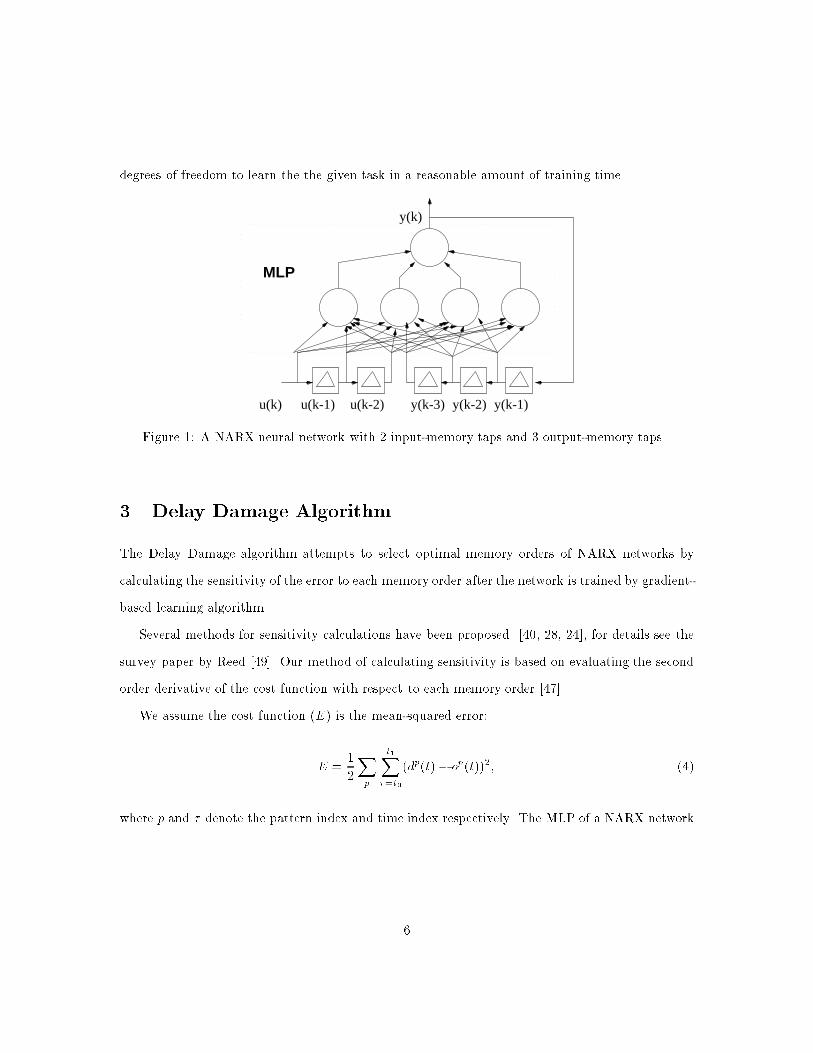
degrees of freedom to learn the the given task in a reasonable amount of training time.y(k-1)y(k-2)y(k-3)u(k-1)u(k) u(k-2)

MLP

y(k)

Figure 1: A NARX neural network with 2 input-memory taps and 3 output-memory taps.3 Delay Damage AlgorithmThe Delay Damage algorithm attempts to select optimal memory orders of NARX networks bycalculating the sensitivity of the error to each memory order after the network is trained by gradient-based learning algorithm.Several methods for sensitivity calculations have been proposed [40, 28, 24], for details see thesurvey paper by Reed [49]. Our method of calculating sensitivity is based on evaluating the secondorder derivative of the cost function with respect to each memory order [47].We assume the cost function (E) is the mean-squared error:E = 12Xp t1X�=t0(dp(t) � op(t))2; (4)where p and � denote the pattern index and time index respectively. The MLP of a NARX network6

can be described as: xi(t) = f (ai(t)) ; (5)ai(t) = Xj wijxj(t); (6)where xi(t) is the output of hidden node i, ai(t) is the weighted-sum input, f is the nonlinearfunction, and wij is the real valued connection weight from node j to node i.By the chain rule, the �rst-order derivative of E with respect to output node i at time t = t1 isgiven as @E@ak(t1) = f 0k(ak(t1))ek(t1); (7)where ek(t1) is the error between the output node and the target output. The gradient informationof the hidden nodes can be obtained by backpropagating the gradient information from the outputnode. For the earlier time steps, there will be an injection error from the target output into theoutput node. Thus, not only is the gradient information determined by a backward pass throughthe unrolled network, but the injection errors are also taken into account in reverse order. The errorsignal of output node k at time t0 < � < t1 will become:@E@ak(� ) = f 0k(ak(� ))0@ek(� ) +Xj wjk @E@ak(� + 1)1A : (8)Di�erentiating the �rst-order derivative once more yields the second order information. For theoutput node k at the last time step t1, the second order information can be described by@2E@a2k(t1) = f 0(ak(t1))2 � ek(t1)f 00(aK(t1)): (9)The Levenberg-Marquardt approximation was used by Le Cun et al. to drop the second term ofEquation 9. This will result in the same order of complexity as computing the �rst-order derivatives7

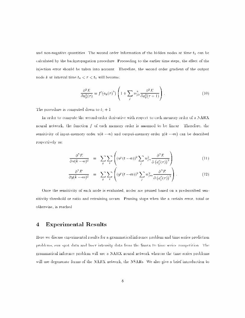
and non-negative quantities. The second order information of the hidden nodes at time t1 can becalculated by the backpropagation procedure. Proceeding to the earlier time steps, the e�ect of theinjection error should be taken into account. Therefore, the second order gradient of the outputnode k at interval time t0 < � < t1 will become:@2E@a2k(� ) = f 0(ak(� )2)0@1 +Xj w2jk @2E@a2k(� + 1)1A : (10)The procedure is computed down to t0 + 1.In order to compute the second-order derivative with respect to each memory order of a NARXneural network, the function f of each memory order is assumed to be linear. Therefore, thesensitivity of input-memory order u(k � n) and output-memory order y(k � m) can be describedrespectively as: @2E@u(k � n)2 = Xp X� 0@(up(t � n))2Xj w2jn @2E@ �apj (� )�21A (11)@2E@y(k �m)2 = Xp X� 0@(yp(t�m))2Xj w2jm @2E@ �apj (� )�21A : (12)Once the sensitivity of each node is evaluated, nodes are pruned based on a predescribed sen-sitivity threshold or ratio and retraining occurs. Pruning stops when the a certain error, total orotherwise, is reached.4 Experimental ResultsHere we discuss experimental results for a grammatical inference problem and time series predictionproblems, sun spot data and laser intensity data from the Santa Fe time series competition. Thegrammatical inference problem will use a NARX neural network whereas the time series problemswill use degenerate forms of the NARX network, the NSARs. We also give a brief introduction to8

the theory of dynamic embedding before discussing the results of time series prediction.In order to also optimize the architecture of the MLP of a NARX network or NSAR, severalmethods of weight-elimination [5, 29, 44, 61, 63] can be incorporated into the training algorithm.In the following experiments, networks are trained using weight decay [29]. All experiments weretrained using Back-Propagation Through Time (BPTT).4.1 Grammatical Inference: Learning A 512-state Finite Memory Ma-chineNARX networks have been shown to be able to simulate and learn a class of �nite state machines [8,21], called respectively de�nite and �nite memory machines. When being trained on strings whichare encoded as temporal sequences, NARX networks are able to \learn" rather large (hundreds tothousands of states) machines provided that they have enough memory and the logic implementationis not too complex. However, the generalization performance and the size of extracted machinesare also found to be very sensitive to the memory order selections in NARX networks [35]. Thepurpose of this experiment is to see how the delay damage algorithm can improve the generalizationperformance of NARX networks with unnecessary memory structures.In this experiment, the �nite memory machine has 512 states. The machine has input order of5 and output order of 4. Its transition function can be described as the simple logic function:y(k) = �u(k � 5)�u(k) + �u(k � 5)y(k � 4) + u(k)u(k � 5)�y(k � 4) (13)where y and u represent output and input respectively, and �x represents the complement of x. TheFSM is shown in Figure 2. The depth, d, of the machine is 9. The training set was 300 stringsrandomly chosen from the complete set. The complete set, which consists of all strings of lengthfrom 1 to d+1 (10 in this case), are shown to be able to su�ciently identify a �nite memory machinewith depth d [20] . The strings were encoded such that input values of 0s and 1s and target outputlabels \negative" and \positive" corresponded to oating point values of 0:0 and 1:0 respectively.9

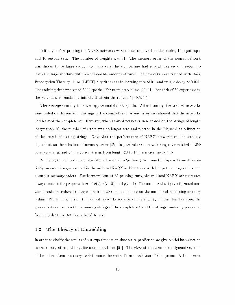
Initially, before pruning the NARX networks were chosen to have 4 hidden nodes, 10 input taps,and 10 output taps. The number of weights was 91. The memory order of the neural networkwas chosen to be large enough to make sure the architecture had enough degrees of freedom tolearn the large machine within a reasonable amount of time. The networks were trained with BackPropagation Through Time (BPTT) algorithm at the learning rate of 0:1 and weight decay of 0:001.The training time was set to 5000 epochs. For more details, see [20, 21]. For each of 50 experiments,the weights were randomly initialized within the range of [�0:5; 0:5].The average training time was approximately 600 epochs. After training, the trained networkswere tested on the remaining strings of the complete set. A zero error rate showed that the networkshad learned the complete set. However, when trained networks were tested on the strings of lengthlonger than 10, the number of errors was no longer zero and plotted in the Figure 3 as a functionof the length of testing strings. Note that the performance of NARX networks can be stronglydependent on the selection of memory order [35]. In particular the new testing set consisted of 250positive strings and 250 negative strings from length 20 to 150 in increments of 10.Applying the delay damage algorithm described in Section 3 to prune the taps with small sensi-tivity measure always resulted in the minimal NARX architectures with 5 input memory orders and4 output memory orders. Furthermore, out of 50 pruning runs, the minimal NARX architecturesalways contain the proper subset of u(t), u(t�5), and y(t�4). The number of weights of pruned net-works could be reduced to anywhere from 20 to 30 depending on the number of remaining memoryorders. The time to retrain the pruned networks took on the average 70 epochs. Furthermore, thegeneralization error on the remaining strings of the complete set and the strings randomly generatedfrom length 20 to 150 was reduced to zero.4.2 The Theory of EmbeddingIn order to clarify the results of our experiments on time series prediction we give a brief introductionto the theory of embedding, for more details see [51]. The state of a deterministic dynamic systemis the information necessary to determine the entire future evolution of the system. A time series10

Figure 2: A 512 state �nite memory machine with input order 5 and output order 4.20 40 60 80 100 120 1400

10

20

30

40

50

60

70

80

90

100

Lenth of testing strings

Num

ber

of e

rror

s in

the

test

ing

set

Figure 3: Number of errors in the testing set, which consists 250 positive strings and 250 negativestrings from length 20 to 150, as a function of the length of the strings for a NARX neural networktrained on the data from the 512 state �nite memory machine.11

is a set of measures of an observable quantity of the system over time. An observable quantity is afunction only of the state of the underlying system. The observations , y(n), are a projection of themultivariate state space of the system onto the one dimensional space. In order to do prediction, weneed to reconstruct as well as possible the state space of the system using the information in y(n).The embedding theorem motivates the technique of using time-delay coordinate reconstructionin reproducing the phase space of an observed dynamical system. A collection of time lags in avector space of d dimensions,s(t) = hy(t); y(t � T ); y(t � 2T ); � � � ; y(t� (d� 1)T )i ; (14)will provide su�cient information to reconstruct the states of the dynamical system. The purposeof time-delay embedding is to unfold the projection back to a multivariate state space that is rep-resentative of the original system [43, 46, 57]. It was shown that if the dynamical system and theobserved quantity were generic, then the delay coordinate map from a d-dimensional smooth compactmanifold to 2d + 1-dimensional reconstruction space was a di�eomorphism (one-to-one di�erentialmapping). The theorem was further re�ned by Sauer et al. [51] such that a measured quantity led toa one-to-one delay coordinate map as long as the reconstruction dimension was greater than twicethe box-counting dimension of the attractor. The embedding theorem provides a su�cient conditionfor choosing the embedded dimension dE large enough so that the projection is theoretically able toconstruct the original state space. Once a large enough d = dE has been obtained, any d � dE willalso provide an embedding.The predictive relationship between the current state s(t) and the next value of time series canbe expressed as y(t + 1) = f (s(t))= f (y(t); y(t � T ); y(t � 2T ); � � � ; y(t � (d� 1)T )) : (15)12

The embedding theorem provides a theoretical framework for nonlinear time series prediction.Once an embedding dimension is chosen, one remaining task is to approximate the mapping func-tion f . It has been shown that a feedforward neural network with enough neurons is capable ofapproximating any nonlinear function to an arbitrary degree of accuracy [12, 19, 26, 27]. Neuralnetworks thus can provide a good approximation to the function f . These arguments provide thebasic motivation for the use of NARX networks to the nonlinear time series prediction.It is still an open question as to how to optimally choose the embedding dimension d and thedelay time T . The embedding theorem only guarantees that a su�ciently large embedding dimensiondE will be capable of unfolding the state space. It does not describe how complicated the mappingfunction will be. One may be able to �nd a minimum embedding dimension to unfold the statespace, but the mapping function may be too complicated to approximate. For example, two di�erentembedded dimensions can be equivalent in terms of repressive power, but the nonlinear function maydramatically di�er in the e�ciency of approximation. It should be noted that when T is chosen,the embedding representation will always be equally spaced. This rules out the possibility of anyunequally spaced representation of the embedding dimension.In the following experiments, we will use the delay damage algorithm to prune the taps of aneural network. After pruning, the networks will be retrained, at least twice. The �nal networkarchitecture ends up providing a unequally spaced temporal representation of the state space. Thesesparse delay architectures can be regarded as the nonlinear versions of SAR models (NSARs) and thesubset orders of the NSAR provide the embedding coordinates to reconstruct the mapping function.The time lags in the initial embedding vector can be equally or unequally spaced as long as theembedding dimension is large enough to unfold the state space.4.3 Prediction of Sunspot DataSunspots are dark botches on the sun and yearly averages have been recorded since 1700. The seriesis shown in Figure 4 and has served as a benchmark for time series prediction problems. Severalresearchers have tested the prediction ability of neural networks on this data. For example, Weigend13

et al. [61] trained a NSAR (or TDNN) network with an embedded dimension of 12 with 8 hiddenneurons and pruned the weights by adding a complexity term to the cost function. They were ableto reduce a network with 8 hidden nodes to 3. The embedding dimension remained the same. Svareret al. [56] pruned the weights using a second order sensitivity measure. Our approach is to prune theorders of networks directly and use the weight decay technique to optimize the nonlinear mappingfunction.For comparison we treat the data in the same way as Weigend et al. [61]. and partition it into atraining set from 1700 through 1920 and a testing set from 1921 to 1979. The data set was scaled tobe in the range of [0; 1:0]. We tried various architectures with various number of hidden nodes anddi�erent embedding dimensions. The initial embedding dimension was usually close to 14. However,the largest initial order depth was 33. The networks were trained as a one-step ahead predictorsat the learning rate of 0:1 and weight decay of 0:001. After pruning the taps, the networks wereretrained.Our cost function was the normalized mean squared error de�ned as:NMSE(N ) = Pk2S (targetk � predictionk)2Pk2S (targetk �meanS )2= 1�2 1N Xk2S(xk � x̂k)2; (16)where k = 1 � � �N enumerates the point in the data set S, and meanS and �2 denote the sampleaverage and sample variance of the target value in S. This measure removes the data's dependenceon dynamic range and size of the data set. To make comparisons with previous work, the variancewas normalized with the same value of 1535 [61]. Training was stopped when the normalized meansquared error was less than 0:1.Reported in table 1 are our two best results from the architectures denoted as B and C. The�nal number of hidden nodes were respectively 6 and 3. The �nal subset orders of the two net-works after pruning consisted of (xt; xt�1; xt�9; xt�11; xt�13; xt�14; xt�31; xt�33) and (xt; xt�1; xt�2;xt�8; xt�10; xt�11; xt�19; xt�22) respectively. Table 1 lists the one-step ahead prediction performance14

Network NMSE No. of parametersTrain (1700-1920) Test (1921-1955) Test (1956-1979)A (Weigend et al.) 0.082 0.086 0.35 43B 0.094 0.1065 0.449 69C 0.0966 0.1013 0.4033 31D (Svarer et al. ) 0.090 0.082 0.35 14Table 1: Normalized MSE for one-step ahead prediction on the sunspot data.of various models on the data set. Comparing the NMSE, the single-step prediction qualities of dif-ferent models are quite comparable.We also compared long-term prediction results to one another. To do the long-term prediction,the predicted output is fed back into the neural network. Hence, the inputs consists of predictedvalue as opposed to actual data of the origin time series. We used the average relative I-timesiterated prediction variance proposed by Weigend et al. [61] as a performance measure of the long-term behavior of the models. The average relative I-times iterated prediction variance is de�nedas: arv(iterated; I) = 1�2 1M MXt=1(xt � x̂t;I)2; (17)where xt is the real data point at time t, M the di�erence between the period of the prediction andI, and x̂t;I is the predicted value for time t after I iterations. Recall that I is the number of timesteps into the future of the prediction. The average relative iterated prediction variance is shown inFigure 5 and went through from 1921 to 1979. From Figure 5, it can be seen that the networks Band C which have sparsely connected tapped delay lines start to perform better as I is increased.Note that the arv is greater than 1:0, since the variance of the original data 1920 through 1979 isfairly large. If we normalize the arv to the variance of the original data set, the results are shown inFigure 6. Again the networks B and C perform better as I is increased.15

0

20

40

60

80

100

120

140

160

180

200

1700 1750 1800 1850 1900 1950

Yea

rly s

unsp

ot a

vera

ges

YearFigure 4: Sunspot data for years 1700 to 1979.A

B

C

D

0 5 10 15 20 25 300.4

0.6

0.8

1

1.2

1.4

1.6

Number of iterations

Arv

Relative multi−step prediction performance

Figure 5: Relative multi-step prediction performance. These results were normalized to a varianceof 1535. 16

A

B

C

D

0 5 10 15 20 25 300.2

0.3

0.4

0.5

0.6

0.7

0.8

0.9

Number of iterations

Arv

Multi−step performance

Figure 6: Relative multi-step prediction performance. The results were normalized to the varianceof the original data set.4.4 Prediction of Laser DataIn order to explore the capability of capturing the global behavior of NSAR neural networks, wealso tested them on the laser data the Santa Fe competition. The data set consists of laser intensitycollected from a laboratory experiment [62]. Although deterministic, its behavior is chaotic as seenin Figure 7. Figure 8 shows the normalized autocorrelation function of the �rst 1000 training datapoints.The networks were trained as a one-step ahead predictor using the �rst 1000 points. The data wasscaled to zero mean and unit variance. We give the results of our best performing neural network.The network was chosen to have two hidden layers. The �rst hidden layer had 5 neurons and thesecond layer had 3 neurons. We used the hyperbolic tangent function as the nonlinear function inthe two hidden layers. The output layer had only one output neuron with linear function. We chosethe embedding dimension to be 25. However, the depth of the tapped delay line was very long (upto 500). We used the last 12 subsets, 3 subsets from the past 100 data points (i.e., xt�99,xt�100,17

xt�101), and 10 subsets from the past 445 data points (i.e., xt�445,� � � ,xt�455). We heuristicallychose the memory order by observing that the autocorrelation function of the training data set waspeaked in these areas. The total number of weights was 152.In this experiment, we used the adaptive learning rate algorithm and batch data presentation.The algorithm works as follows. The cost function is monitored during training. If the increase ofthe cost function at time t is not larger than the product of the cost of previous time step and the costbonus, �, the learning rate is increased by ten percent until the learning rate reaches the maximumlearning rate, 1:0, and the weights are updated. If the increase of the cost function at the presenttime step is larger than the product of the cost bonus and the cost of earlier time step, the weightvector of previous time step is restored and the learning rate decreases by half until it reaches theminimum learning rate (10�8), and the weights are updated according to the smaller learning rateand the gradient information of one time step ahead. Of course, this requires one to keep track ofthe weight vector and the gradient information of previous time steps. In our experiment, the initiallearning rate was 0:01 and the cost bonus, �, was 0:001. The network was trained with the previouslydiscussed mean squared error cost function in the batch mode (i.e. errors were accumulated untilthe end of the data). When the average squared error is less than 0.004, training was stopped andpruning commenced. This procedure was performed twice.The trained and pruned neural network NSAR gave some interesting long-term predictive behav-ior of the time series. The network was able to predict 1000 data points using closed-loop iteration.Figure 9 shows the 500 steps iterated prediction from time t = 1000. Figure 10 shows the 1000 stepiterated prediction; note that the network was able to predict three collapses and there were onlytwo collapses in the training data set. We pruned 5 taps of the original network when trained onthe �rst 1000 data points. The �nal architecture had only 127 weights.18

0

50

100

150

200

250

300

0 100 200 300 400 500 600 700 800 900 1000Figure 7: Original 1000 laser data.0 100 200 300 400 500 600 700 800 900 1000

−0.8

−0.6

−0.4

−0.2

0

0.2

0.4

0.6

0.8

1

Lag

Normalized Autocorrelation

Figure 8: Normalized autocorrelation function of the 1000 laser data.19

-50

0

50

100

150

200

250

300

1000 1050 1100 1150 1200 1250 1300 1350 1400 1450 1500Figure 9: The solid line represents 500 data points predicted by the pruned network when usingclosed loop iteration.20

-100

-50

0

50

100

150

200

250

300

1000 1100 1200 1300 1400 1500 1600 1700 1800 1900 2000

Figure10:Thesolidlinerepresents1000datapointspredictedbytheprunednetworkwhenusingclosedloopiteration.

21

5 ConclusionDetermining of the proper architecture of a dynamical network is a di�cult yet critical task. Not onlycan the nonlinear architectures a�ect the performance, but the memory architecture of dynamicalmodel can have a signi�cant impact on its dynamical behavior.In this paper, we proposed a pruning-based algorithm to determine the embedded memory orderof NARX recurrent neural networks and degenerate forms such as NSAR networks. This algorithmcan also incorporate several useful heuristics, e.g. weight decay, which have been used extensively instatic networks to optimize the nonlinear function. We also show that this algorithm can demonstrateimproved performance on both nonlinear predictions and grammatical inference tasks. Furthermore,optimizing the memory architecture and the nonlinear function through pruning often results insparsely connected architectures but with long time windows which are able to model the globalfeatures of the underlying system quite e�ciently.Though the embedding theorem demonstrates that the order of embedded memory should belarge enough in order to provide a guarantee of forming a di�eomorphism mapping, choosing theproper memory order can be a challenge. Choosing di�erent embedding memory architecturescorresponds to giving di�erent representations of the state space of the underlying system. Themajor issue is that such a representation plays an important role in solving problems. A goodrepresentation can make useful information explicit and easy to extract. In this work we onlyexplored classic tapped delay memory structures. It would be interesting to see if similar resultscould be achieved for other memory models[3, 59]. However, a minimal representation does notnecessarily mean a good representation. Two di�erent representations can be equivalent in terms ofexpressive power, but may make a great di�erence in e�ciency and e�ectiveness of problem-solving.6 AcknowledgementsWe would like to acknowledge useful discussions with G. Flake, D. Hush and J. Principe.22

References[1] H. Akaike. A new look at the statistical model identi�cation. IEEE trans. Automatic Control,AC 19:716{723, 1974.[2] W. Atmar. Notes on the simulation of evolution. IEEE Transactions on Neural Networks,5(1):130{148, 1994.[3] A.D. Back and A.C. Tsoi. A comparison of discrete-time operator models for nonlinear sys-tem identi�cation. In G. Tesauro, D. Touretzky, and T. Leen, editors, Advances in NeuralInformation Processing Systems 7, pages 883{890. MIT Press, 1995.[4] U. Bodenhausen and A. Waibel. The tempo 2 algorithm: Adjusting time-delays by supervisedlearning. In Advances in Neural Information Processing Systems 3, pages 155{161. MorganKaufmann, San Mateo, CA, 1991.[5] Y. Cauvin. A back-propagation algorithm with optimal use of hidden units. In D. Touretzky,editor, Advances in Neural Information Processing Systems 1, pages 519{526, 1989.[6] S. Chen, S.A. Billings, and P.M. Grant. Non{linear system identi�cation using neural networks.International Journal of Control, 51(6):1191{1214, 1990.[7] Yung-Fu Cheng and Delores M. Etter. Analysis of an adaptive technique for modeling sparsesystems. IEEE Transactions on Acoustics, Speech, and Signal Processing, 37(2):254{264, 1989.[8] D.S. Clouse, C.L. Giles, B.G. Horne, and G.W. Cottrell. Time-delay neural networks: Rep-resentation and induction of �nite state machines. IEEE Transactions on Neural Networks.Accepted.[9] J. Connor, L.E. Atlas, and D.R. Martin. Recurrent networks and NARMA modeling. In J.E.Moody, S.J. Hanson, and R.P. Lippmann, editors, Advances in Neural Information ProcessingSystems 4, pages 301{308, 1992.[10] Y. Le Cun, J. S. Denker, and S. A. Solla. Handwritten digit recognition with a backpropagationnetwork. InAdvances in Neural Information Processing Systems, volume 2, pages 396{404, 1990.[11] Y. Le Cun, J. S. Denker, and S. A. Solla. Optimal brain damage. In D.S. Touretzky, editor,Advances in Neural Information Processing Systems, volume 2, pages 598{605, San Mateo, CA,1990. Morgan Kaufmann Publishers.[12] G. Cybenko. Approximation by superpositions of a sigmoidal function. Mathematics of Control,Signals, and Systems, 2(4):303{314, 1989.[13] J. E. Dayho� D.-T. Lin and P. A. Ligomenides. A learning algorithm for adaptive time-delaysin a temporal neural network. Technical Report SRC-TR-92-59, Systems Research Center,University of Maryland, College Park, Maryland, 1992.[14] Shawn P. Day and Michael R. Davenport. Continuous-time temporal back-propagation withadaptable time delays. IEEE Transactions on Neural Networks, 4(2):348{354, 1993.23

[15] D. M. Etter and S. D. Stearns. Adaptive estimation of time delays in sampled data systems.IEEE Transactions on Acoustics, Speech, and Signal Processing, ASSP-29(3):582{587, 1981.[16] David B. Fogel. An information criterion for optimal neural network selection. IEEE Transac-tions on Neural Networks, 2(5):490{497, 1991.[17] David B. Fogel. Using evolutionary programming for modeling: An ocean acoustic example.IEEE Journal of Oceanic Engineering, 17(4):333{340, 1992.[18] David B. Fogel. Evolutionary programming: An introduction and some current directions.Statistics and Computing, 4:113{129, 1994.[19] K. Funahashi. On the approximate realization of continuous mappings by neural networks.Neural Networks, 2(3):183{192, 1989.[20] C. L. Giles, B. G. Horne, and T. Lin. Learning a class of large �nite state machines with arecurrent neural network. Technical Report UMIACS{TR{94{94 and CS{TR{3328, Institutefor Advanced Computer Studies, University of Maryland, College Park, Maryland, 1994.[21] C.L. Giles, B.G. Horne, and T. Lin. Learning a class of large �nite state machines with arecurrent neural network. Neural Networks, 8(9):1359{1365, 1995.[22] C.L. Giles and C.W. Omlin. Pruning recurrent neural networks for improved generalizationperformance. IEEE Transactions on Neural Networks, 5(5):848{851, 1994.[23] E. J. Hannan and B. G. Quinn. The determination of the order of an autoregression. J. RoyalStat. Soc. B., 41:190{195, 1979.[24] Babak Hassibi and David G. Stork. Second order derivatives for network pruning: Optimal brainsurgeon. In S.J. Hanson, J.D. Cowan, and C.L. Giles, editors, Advances in Neural InformationProcessing Systems 5, San Mateo, CA, 1993. Morgan Kaufmann Publishers.[25] B.G. Horne and C.L. Giles. An experimental comparison of recurrent neural networks. InAdvances in Neural Information Processing Systems 7, pages 697{704. MIT Press, 1995.[26] K. Hornik, M. Stinchcombe, and H. White. Multilayer feedforward networks are universalapproximators. Neural Networks, 2(5):359{366, 1989.[27] B. Irie and S. Miyake. Capabilities of three{layered perceptrons. In Proceedings of the IEEEInternational Conference on Neural Networks, volume 1, pages 641{648, San Diego, CA, 1988.IEEE.[28] E.D. Karnin. A simple procedure for pruning back{propagation trained neural networks. IEEETransactions on Neural Networks, 1(2):239{242, 1990.[29] A. Krogh and J.A. Hertz. A simple weight decay can improve generalization. In J.E. Moody,S.J. Hanson, and R.P. Lippmann, editors, Advances in Neural Information Processing Systems4, pages 950{957, 1992.[30] K.J. Lang, A.H. Waibel, and G.E. Hinton. A time{delay neural network architecture for isolatedword recognition. Neural Networks, 3(1):23{44, 1990.24

[31] A. Lapedes and R. Farber. Nonlinear signal processing using neural networks: Prediction andsignal modeling. Technical Report LA{UR{87{2662, Los Alamos National Laboratories, LosAlamos, New Mexico, 1987.[32] I.J. Leontaritis and S.A. Billings. Input{output parametric models for non{linear systems: PartI: deterministic non{linear systems. International Journal of Control, 41(2):303{328, 1985.[33] D.T. Lin, J.E. Dayho�, and P.A. Ligomenides. Trajectory production with the adaptive time-delay neural network. Neural Networks, 8(3):447{461, 1995.[34] T. Lin, B.G. Horne, P. Tino, and C.L. Giles. Learning long-term dependencies in narx recurrentneural networks. IEEE Transactions on Neural Networks, 7(6):1329{1338, 1996.[35] Tsungnan Lin, B.G. Horne, and C.L. Giles. How memory orders e�ect the performance ofnarx networks. Technical Report UMIACS-TR-96-76 and CS-TR-3706, Institute for AdvancedComputer Studies, University of Maryland, College Park, Maryland, 1996.[36] Tsungnan Lin, B.G. Horne, P. Tino, and C.L. Giles. Learning long-term dependencies is notas di�cult with narx recurrent neural networks. In Advances in Neural Information ProcessingSystems 8. MIT Press, Cambridge, MA, 1996.[37] L. Ljung. System identi�cation : Theory for the user. Prentice-Hall, Englewood Cli�s, NJ,1987.[38] G. A. N. Mbamalu and M. E. El-Hawary. Load forecasting via suboptimal seasonal autoregres-sive models and iteratively reweighted least squares estimation. IEEE Transactions on PowerSystems, 8(1):343{348, 1993.[39] D.C. Montgomery and E.A. Peck. Introduction to Linear Regression Analysis. Wiley, NewYork, 1982.[40] M. C. Mozer and P. Smolensky. Skeletonization: A technique for trimming the fat from anetwork via relevance assessment. Connection Science, 11:3{26, 1989.[41] K.S. Narendra and K. Parthasarathy. Identi�cation and control of dynamical systems usingneural networks. IEEE Trans. on Neural Networks, 1(1):4{27, 1990.[42] Gil Nave and Arnon Cohen. Ecg compression using long-term prediction. IEEE Transactionson Biomedical Engineering, 40(9):877{885, 1993.[43] R. Ma n�e. On the dimension of the compact invariant sets of certain nonlinear maps. In LectureNotes in Math. No. 898, page 230. Springer-Verlag, 1981.[44] S.J. Nowlan and G.E. Hinton. Simplifying neural networks by soft weight-sharing. NeuralComputation, 4(4):473{493, 1992.[45] Edward Ott, Tim Sauer, and James Yorke. Coping with Chaos. John Wiley and Sons, Inc, NewYork, NY, 1994.[46] N. Packard, J. Crutch�eld, D. Farmer, and R. Shaw. Geometry from a time series. PhysicalReview Letter, 45:712{715, 1980. 25

[47] M.W. Pedersen and L.K. Hansen. Recurrent networks: Second order properties and pruning.In G. Tesauro, D. Touretzky, and T. Leen, editors, Advances in Neural Information ProcessingSystems 7. MIT Press, 1995.[48] S.-Z. Qin, H.-T. Su, and T.J. McAvoy. Comparison of four neural net learning methods fordynamic system identi�cation. IEEE Transactions on Neural Networks, 3(1):122{130, 1992.[49] Russel Reed. Pruning algorithms| a survey. IEEE Transactions on Neural Networks, 4(5):740{747, 1993.[50] J. Rissanen. Universal coding, information, prediction, and estimation. IEEE Transactions onInformation Theory, IT-30:629{636, 1984.[51] T. Sauer, J. Yorke, and M. Casdagli. Embedology. Journal of Statistical Physics, 65:579{616,1991.[52] R. Shibata. Various model selection techniques in time series analysis. In Handbood of statistics,volume 5, pages 179{187. Eds. Amsterdam: Elsevier, 1985.[53] H.T. Siegelmann, B.G. Horne, and C.L. Giles. Computational capabilities of recurrent narxneural networks. IEEE Trans. on Systems, Man and Cybernetics, 1997. In press.[54] H.-T. Su and T.J. McAvoy. Identi�cation of chemical processes using recurrent networks. InProceedings of the American Controls Conference, volume 3, pages 2314{2319, 1991.[55] H.-T. Su, T.J. McAvoy, and P. Werbos. Long{term predictions of chemical processes usingrecurrent neural networks: A parallel training approach. Industrial Engineering and ChemicalResearch, 31:1338{1352, 1992.[56] C. Svarer, L. K. Hansen, and J. Larsen. On design and evaluation of tapped-dealy neuralarchitectures. In IEEE International Conf. on Neural Networks, pages 46{51, 1992.[57] F. Takens. Detecting strange attractors in turbulence. In Lecture Notes in Math. No. 898,pages 366{381. Springer-Verlag, 1981.[58] S.T. Venkataraman. On encoding nonlinear oscillations in neural networks for locomotion. InProceedings of the Eighth Yale Workshop on Adaptive and Learning Systems, pages 14{20, 1994.[59] Bert de Vries and Jose Principe. The gamma model - a new neural network for temporalprocessing. Neural Networks, 5(4):565{576, 1992.[60] A. Waibel, T. Hanazawa, G. Hinton, K. Shikano, and K. Lang. Phoneme recognition usingtime{delay neural networks. IEEE Transactions on Acoustics, Speech and Signal Processing,37(3):328{339, 1989.[61] Andreas S. Weigend, Bernardo A. Huberman, and David E. Rumelhart. Prediction the future:A connectionist approach. International Journal of Neural Systems, 1(3):193{209, 1990.[62] A.S. Weigend and N.A. Gershenfeld. Time Series Prediction: Forecasting the future and un-derstanding the past. Addison{Wesley, 1994.26

[63] A.S. Weigend, B.A. Huberman, and D.E. Rumelhart. Predicting sunspots and exchange rateswith connectionist networks. In M. Casdagli and S. Eubank, editors, Nonlinear Modeling andForecasting, SFI Studies in the Sciences of Complexity, volume 12. Addison{Wesley, 1991.[64] Gwo-Hsing Yu and Yow-Chano Lin. A methodology for selecting subset autoregressive timeseries models. Journal of Time Series Analysis, 12(4):363{373, 1989.

27