HIGH-FREQUENCY GAS-DISCHARGE BREAKDOWN IN HELIUM

A. D. MacDONALD and SANBORN C. BROWN

TECHNICAL REPORT NO. 86

OCTOBER 23, 1948

RESEARCH LABORATORY OF ELECTRONICS

MASSACHUSETTS INSTITUTE OF TECHNOLOGY

II4i

The research reported in this document was made possiblethrough support extended the Massachusetts Institute of Tech-nology, Research Laboratory of Electronics, jointly by the ArmySignal Corps, the Navy Department (Office of Naval Research)and the Air Force (Air Materiel Command), under Signal CorpsContract No. W36-039-sc-32037, Project No. 102B; Departmentof the Army Project No. 3-99-10-022.

MASSACHUSETTS INSTITUTE OF TECHNOLOGY

Research Laboratory of Electronics

Technical Report No. 86 October 23, 1948.

HIGH-FREQUENCY GAS-DISCHARGE BREAKDOWN IN HELIUM

A. D. MacDonald and Sanborn C. Brown

Abstract

Breakdown electric fields in low-pressure helium at high fre-quencies have been theoretically predicted and experimentally verified.The energy distribution of electrons is derived from the Boltzmann trans-port equation by taking into account all significant removal processes. Thedistribution function is expanded in spherical harmonics and the resultingsecond-order linear differential equation is solved in terms of the con-fluent hypergeometric function. This distribution function combined withkinetic theory formulas permits calculation of the ionization rate and theelectron diffusion coefficient. From these the high-frequency ionizationcoefficient is determined. Through the diffusion equation this ionizationcoefficient is related to breakdown electric fields. Thus breakdown elec-tric fields are predicted theoretically without using any gas-dischargedata other than experimental values of the excitation potential and col-lision cross section of helium. Breakdown electric fields are measuredfor helium in microwave cavities of various sizes with a large range ofpressure. The theoretical electric fields, involving no adjustable param-eters, are checked within the maximum experimental error of 6 per cent.

HIGH-FREQUELNCY GAS-DISCHARGE BREAKDOWN IN HELIUM

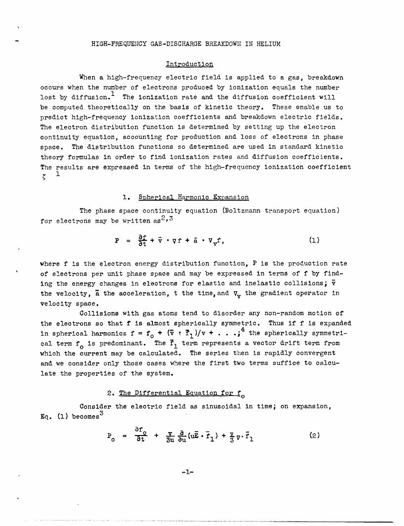
Introduction

When a high-frequency electric field is applied to a gas, breakdown

occurs when the number of electrons produced by ionization equals the number

lost by diffusion.1 The ionization rate and the diffusion coefficient will

be computed theoretically on the basis of kinetic theory. These enable us to

predict high-frequency ionization coefficients and breakdown electric fields.

The electron distribution function is determined by setting up the electron

continuity equation, accounting for production and loss of electrons in phase

space. The distribution functions so determined are used in standard kinetic

theory formulas in order to find ionization rates and diffusion coefficients.

The results are expressed in terms of the high-frequency ionization coefficient

1. Spherical Harmonic Expansion

The phase space continuity equation (Boltzmann transport equation)

for electrons may be written as2,3

P = a+ + Vf, (1)

where f is the electron energy distribution function, P is the production rate

of electrons per unit phase space and may be expressed in terms of f by find-

ing the energy changes in electrons for elastic and inelastic collisions; v

the velocity, the acceleration, t the time,and Vv the gradient operator in

velocity space.

Collisions with gas atoms tend to disorder any non-random motion of

the electrons so that is almost spherically symmetric. Thus if f is expanded

in spherical harmonics f = fo + ( ? 1l)/v + . . .;4 the spherically symmetri-

cal term f is predominant. The ?l term represents a vector drift term from

which the current may be calculated. The series then is rapidly convergent

and we consider only those cases where the first two terms suffice to calcu-

late the properties of the system.

2. The Differential Euation for fo

Consider the electric field as sinusoidal in time; on expansion,

Eq. (1) becomes3

afo aP = at + 3u auE l) + 3°V l (2)

-1-

..1""~ .. ~~1 ~~~~1-_-I , · _ -

anda- aratl afo

P1 a-- + vVf + vi au (3)

provided P is expanded P = Po + (Pl.v)/v, and the electric field is represented

by E. An energy variable u is introduced by setting mvy /2e = u, where e

is the electronic charge and m is the mass of the electron.

Elastic collisions may be considered as instantaneous processes and

the energy loss therefrom may be treated by putting equivalent loss terms

P oel and 1,el in the equation. Morse, Allis, and Lamar3 have shown that

o, el =2 u d (4)

and

Pl,el - , fl' (5)

I being the electronic mean free path, and M the mass of the atom.

In low-pressure helium, recombination is not a significant electron

removal process at breakdown. Ionizations and excitations have no angular

dependence and therefore make a contribution to P only; we represent this

contribution due to inelastic collisions by Po in.

The electric field E is represented by EejWt where w is the radian

frequency. In the gas, the energy transfer by the field to the electrons

depends on E2 so that the root-mean-square field is all that is required.

There follows directly from Margenau's analysis 5 an expression for E fl

which is the same as that obtained by considering an effective field Ee defined

by

E2 = E (/) 2 (6)

where E is the r.m.s. value of the applied field.

The differential equation for fo then becomes

u2f d E2 (v/j . (7)Po,in + d oo f E v !2]Poin M u du( t ) SA2 o 3u du (v/)2 + 2 (7)

Here 2fo has been replaced by (-1/A2 )f0 by using the diffusion equation.l

The factor 1/ 2 depends on the geometry of the discharge container, and is the

-2-

characteristic value in the solution of the diffusion equation; A is then

the characteristic diffusion length. The mean free path equals /(pP) if

p is the pressure and Pc the probability of collision per cm of path per

mm of pressure. There now remains to specify the functional forms of Pc

and Po,in' to complete the formulation of the equation. Excitation will

be effectively eliminated by the introduction of mercury vapor.

3. Expression for the Collision Cross Sections

1A good approximation for Pc in helium is Pcu 2 = constant =

143 volts2/(cm x mm Hg).6 The experimental curve departs from this form for

u less than 4 volts and Pc is roughly constant from u = 0 to u = 4, Most

of the collisions the electron makes with gas atoms'occur after the electron

has an energy of 4 e.v., so that this discrepancy has a small effect on thebreakdown field. The solution of the equation will be carried ot by assum-

1ing Pu 2 = constant over the whole range of electron energies, and will be

corrected in Sec. 5 by finding the distribution function required when this

range of constant mean free path is considered.

Helium has a metastable level at 19.8 volts and transitions from

this level to the ground state by radiation are forbidden. Since metastable

states have mean lives of the order of thousands of microseconds, practi-

cally every helium atom which reaches an energy of 19.8 volts will collide

with a mercury atom and lose its energy by ionizing the mercury. Therefore

each inelastic collision will produce an ionization and the effective ioni-

zation potential ui will be the first helium excitation potential plus a

small overshoot energy due to the fact that the most probable energy at

excitation is higher than the excitation energy. (The amount of this over-

shoot is calculated in Sec. 6.) Then P in may be assumed zero for uui

and infinite for u> ui. Physically this means that there will be no elec-

trons with an energy above that corresponding to u = ui. This condition

on the electron population provides a boundary value for the differential

equation which we now solve for u ui, with fo zero for u = ui.

4. Solution of the Equation and Evaluation of.

Equation (7) becomes, on inclusion of results of Sec.3, in the

region where u< ui

d [u difo -+fdu ' = 0 (8)du L2 '1 P p

-3-

---- . ---

where

z= a m A2 ,M e 2

and

= 1ET)

1r is the mean free time, = 2.37(109 )p(in mm Hg) 6 and

- = 1+ (1)2.

For convenience we transform to a dimensionless independent variable by

letting

w = 1 i+ 4- u = Lb uw-2 P¢ ¢ (9)

and transform the dependent variable by

fo= (g)exp - -( + 1)w .

Then

w d _ - W _ag = dw2 dw'2 _ - = 0

(10)

(11)

where

a = (1 - ).

Equation (11) is the confluent hypergeometric equation7 and its solutions

may be written as8

gl = M(a; ; w) g2 = w- M(a - 1; ; w).

For brevity we will use the notation

M(a; w) = Ml(w)

-4-

(12)

(13)

I

and

w- (a -f 1f2;w) = M2(w). (14)

Then the distribution function fo is given by

f = [Ml () + CM2 (w)] exp I-w(l - 2/3 a)] (15)

where the constant C is determined by the boundary condition that the dis-

tribution function go to zero at u = ui; therefore

C - M2(wi)

Having determined the distribution function we are in a position

to calculate the high-frequency ionization coefficient . By the use of

standard kinetic theory formulas and the distribution function expressed in

Eq. (15) we calculate the quantities n and nD where n is the electron con-

centration, the ionization rate, and D the diffusion coefficient. The

ratio of n to nD divided by the square of the electric field is -.

The kinetic theory formula for the number of inelastic collisions

per electron per second, v, is

2 GonD= - 4T 2ern,=4rr2~. I P du, (16)

v ,in

Ui

where Pin is the production rate of electrons per unit volume of phase

space due to inelastic collisions

The integral in Eq. (16) is an improper integral but Po,in is

transformed through Eq. (7) to a function of f and u. The resulting

rigorous expression is integrated by parts. The integration, subject to

the condition that fo and dfo/du are zero for u = oo , yields

2(E 2 (2)5/2 [3/2 dfo]nv = - -- ) Fu 0- m3 0T m du (17)U = Ui

-5-

^--II.__I·�LLI-I·(-----CI ---- -�

Similarly the diffusion coefficient for electrons, D, is

nD = $2T' (5/2 ) I i . u3/2du (18)3 m 0

The expression for f from Eq. (15) is substituted in the integrand and

the integrations performed. The integrals have been evaluated for arbi-

trary values of the parameters involved.8

On carrying out the integrations in Eq. (18), and dividing

Eq. (17) by the resulting expression we have the high-frequency ioniza-

tion coefficient

= DE2 = (EA)2 M1 (wi) exp( - wi) - 1] (19)V

The form of Eq. (18) has been simplified by using the fact that the

expression

E (Wi) 2(wi) - (wi)Ml(Wi) + 2w il(wi)M2(wi)

is the Wronskian of the differential Eq. (11) and its value isw 3/2 exp Wi. At breakdown v/D = 1/A2, so we see from Eq. (19) that

the breakdown lectric fields may be determined by solving the equation

Ml (wi) exp( - 2 2w i)= 2. (20)

For helium, the numerical values of the variables involved in

terms of experimental parameters are

Wi = 0.20(10 ) bL + ( D) (21)(EkN)2

b (22)

a = 0.75 b- 1 (23)b

-6-

where is the free-space wavelength of the electric field in cm, E is the

r.m.s. value of the electric field in volts per cm, p is the pressure in mm

of Hg and JAis in cm.

A plot of vs.E/p is given in Fig. 1, computed from Eq. (19).

Tables of the functions involved are available.8 The breakdown electric

field may be determined from Fig. 1 by fihding the curve through those

points where = l/( 2E2).

e.ZI

voltsE/p( cmn rn-Hg

Fig. 1. The high-frequency ionization coefficient " computed as a function

of E/p from Eq. (19). The breakdown curve is indicated by the

dashed line; it is determined by setting = 1/ A2E2 ).

5. Correction for Flat Portion of P Curve

From Fig. 2 we see that our approximation for Pc is inaccurate

for electron energies below 4 e.v., and therefore in those cases where

there are many electrons with low energies, a small correction term may be

applied. The low-energy electrons are most important in determining break-

down fields when E/p is small and there are many more collisions per second

than oscillations of the field per second, because under these conditions,

-7-

....... �..�, ��*rrrp·l·l* ·- -··· I· U----·-�l-......�... .1.-1..� �-·�- I---sl----

o)

pc

u

Fig. 2. The probability of collision of electrons in helium at 1 mm ofHg pressure. Brode's experiment is compared with the approximationof this paper.

the relative number of low energy electrons is large. For energies below

4 e.v., Eq. (6) may be simplified by neglecting w2 in comparison with

(v/t)2 , and by using the fact that is constant. The solution may be

carried out in the manner of Sec. 4 and f is then given by

fo = A[M(a;1;y) + BW(a;l;y)] exp(-y) (24)

where M is the confluent hypergeometric function, W is the second solution

for integral values of the second parameter,8'9

a = 1.54(pA)2 '

and

2y = 71.2(s)2 () _

·n b nri

and both functions in Eq. (24) are tabulated.8

-8-

Again we use a more concise notation for the confluent hyper-

geometric function by setting

M(a;l;y) = M3(y)

and

W(a;l;y) = W3 (y).

1The energy at which Pc changes from a constant to a u-T trend

is seen from Fig. 2 to be that corresponding to u ui/5. The distribu-

tion functions in Eqs. (15) and (24) must be smoothly Joined at this energy.

By equating the values and slopes of the distribution functions, the con-

stants A and B are determined to be

...M3 (Yc) - (Yo)B 3 Y 3 Y (25)

W3(yc) - RW3(Yc)

where

1-E ) E °0 [l 2w-..] 3 a a (w) + c (w) [1 - + 3i. i

Ml(Wc) + CM2(c )(26)

and

A [M(w) +OM2 (wc)]eexp[- (l -( _ a)]

[M 3(Y) + BW3 (Yc)]exp (-yc)

This distribution function then modifies the value of the integral for

nD and also the expression for t in Eq. (19).

The amount of this correction for various cavity sizes and

pressures is illustrated in Fig. 3, which shows the correction to be

appreciable only for high pressures, and in no case to be more than a few

per cent.

-9-

��_�__��_1___1___1__I____IPIIBIYII_ _- .-� .. --X�·-_l ·II�IIIYIXI^·�·�C--�-P-·IIII-LYY -I..- -·-.-l.--�____ll�-L·C^IUI-LI--X---111 --·I -- - --- I-

lpOc

1loC'E

'I 10 100 1000p(mmn-Hg)

Fig. 3. Theoretical E - p curves illustrating the effect of the correctionfactors of Secs. 5 and 6. The broken lines indicate theoreticalfields without corrections. The 1/8-in. cavity is omitted to avoidconfusing the diagram.

6. Correction for Overshoot

The probability of excitation is not infinite at the first

excitation potential so that some electrons reach energies above this

value before exciting helium atoms. This overshoot in energy is most

noticeable at low pressures when the energy gained between collisions is

large. To find the energy at which the distribution function goes to zero,10

we insernt the measured values of the excitation function as a loss term

in Eq. (8). The excitation function hx is linear in energy at energies

close to the excitation potential. Using Maier-Leibnitz's experimental

excitation function l o for h, we may write

P 1hx = = h(w - wx ) (u - 198)u2 (28)

c 623

Equation (8) now written in he reduced form and including hx is

- Ig = O fo = (u3/ g)exp(- U ) (29)du2 2

-10-

_- I I111111 11711 1r 1 1 111111 1 I 11

THEORY WITHOUT OVER-S

I I 1 111 1 I I I 111111 I I 11111

IvvCv - ---------|-ova--I

In

where

n 2l hi u.(m hlu + 3) - (30)

For u >ux, I may be seen on inspection to be a slowly varying function so

that we may solve Eq. (30) approximately and obtain

g = exp(- a u). (31)

Equation (31) combined with Eq. (29) gives the distribution function above

the excitation potential; and this distribution function should be fitted

to that of Eq. (15). However, the distribtuion function is small in this

region and we may determine a voltage at which the distribution function

goes to zero by extrapolating Eq. (31) linearly and choosing that voltage

where it cuts the axis as the ionization potential. The extrapolation of

Eq. (31) yields

Ui - ux = g (32)

The effective ionization potential is plotted in Fig. 4 for

helium as a function of E with several values of p, for one value of A/x.

A more rigorous treatment in which Eq. (29) is solved exactly 8 is possible

but does not alter the value of ui in Fig. 4 significantly.

E A (VOLTS)

Fig. 4. The effective ionization potential as a function of E at aconstant ,/.

-11-

�__1__^1�1_11��1_ __------------�----1-----1Ylrrrl__l--··. .-II--I- .I�3sllUI^II��IIYD--Il�--^.·---Llli�-Ll- -._

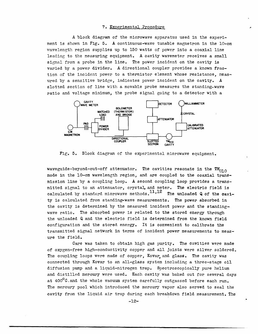
7. Experimental Procedure

A block diagram of the microwave apparatus used in the experi-

ment is shown in Fig. 5. A continuous-wave tunable magnetron in the 10-cm

wavelength region supplies up to 150 watts of power into a coaxial line

leading to the measuring equipment. A cavity wavemeter receives a small

signal from a probe in the line. The power incident on the cavity is

varied by a power divider. A directional coupler provides a known frac-

tion of the incident power to a thermistor element whose resistance, meas-

ured by a sensitive bridge, indicates power incident on the cavity. A

slotted section of line with a movable probe measures the standing-wave

ratio and voltage minimum, the probe signal going to a detector with a

WAVE METER DETECTOR MILLIAMMETERBOLOMETER

MATCHED (THERMISTOR)LOAD AND BRIDGE CRYSTAL

PAD.11W POWER CALIBRATED

0 11 DIVIDER ATTENUATORC.W.

MAGNETRONDIRECTIONAL

COUPLER SLOTTED TMoloSECTION CAVITY

Fig. 5. Block diagram of the experimental microwave equipment.

waveguide-beyond-cut-off attenuator. The cavities resonate in the TM0 1 0

mode in the 10-cm wavelength region, and are coupled to the coaxial trans-

mission line by a coupling loop. A second coupling loop provides a trans-

mitted signal to an attenuator, crystal, and meter. The electric field is

calculated by standard microwave methods. 11 ,12 The unloaded Q of the cavi-

ty is calculated from standing-wave measurements. The power absorbed in

the cavity is determined by the measured incident power and the standing-

wave ratio. The absorbed power is related to the stored energy through

the unloaded Q and the electric field is determined from the known field

configuration and the stored energy. It is convenient to calibrate the

transmitted signal network in terms of incident power measurements to meas-

ure the field.

Care was taken to obtain high gas purity. The cavities were made

of oxygen-free high-conductivity copper and all oints were silver soldered.

The coupling loops were made of copper, Kovar, and glass. The cavity was

connected through Kovar to an all-glass system including a three-stage oil

diffusion pump and a liquid-nitrogen trap. Spectroscopically pure helium

and distilled mercury were used. Each cavity was baked out for several days

at 400 °Cand the whole vacuum system carefully outgassed before each run.

The mercury pool which introduced the mercury vapor also served to seal the

cavity from the liquid air trap during each breakdown field measurement. The

-12-

- --

possible effect of direct ionization of mercury in the breakdown process

has been investigated theoretically. For the density of mercury used it

was found to be not significant in the range of pressures and container

sizes used in the experiment.

The breakdown experiment consists of filling the cavity with the

gas at a measured pressure, increasing the magnetron power until the crystal

current reaches a maximum and drops suddenly to a much lower value. The

drop indicates that the gas has broken down and the maximum current indicates

the breakdown field. The electrons required to initiate the discharge are

provided by a radioactive source near the cavity. The breakdown measurements

were reproducible within an experimental error of less than 5 per cent in

electric field and less than 1 per cent in pressure. Experiments were done

on four cylindrical cavities having a diameter of 8.140 cm and heights of

0.1588, 0.3175, 0.4760, and 2.540 cm. The cavity whose height was great

enough so that it could not be considered a parallel-plate system was conm-

puted using a non-uniform field theory.1 3

Figure 6 presents the experimental and theoretical E vs p curves.

In Fig. 7 vs. E/p curves computed from the experimental data are compared

with theory.

8. Conclusions

The high-frequency ionization coefficient has been calculated

theoretically on the basis of the electron continuity equation by con-

sidering diffusion to the container walls as the only removal process. t

is expressed in terms of EA, p, and pA . The high-frequency ionizationcoefficient has been derived theoretically in Eq. (19). The ionization

coefficient had been previously related to breakdown fields through the

diffusion equation.l

Equation (20), containing no adjustable gas-discharge data or

constants, and involving only the excitation potential and collision cross

section of helium, enables us to predict breakdown electric fields. It has

been derived from the electron velocity distribution function given by

kinetic theory, and the diffusion equation. The agreement between theory

and experiment over a wide range of pressure and container-size variation

verifies the correctness of the approach.

-13-

_ II- ---- -^- -l"-·L~-

r Ii 1 1 1111111 1 1 1111111 I I

-J-J<

Q

a,ao0C

8 da,

0o

00HE H0

*I

H

490)0

a,

tD

.g-iEk.

I11111 I I 111 1111 I 11 1 1

0 0080 . Illiq . -~o

-o .'ILI..~(BsW) d

I _ __ __

ra

6-210

l3

'nc

10

-5

I- I 10 100 1000

E/p ( volts )cm mm-Hg

Fig. 7. Experimental ionization coefficient compared with theoreticallypredicted coefficients. The 1/8-in. cavity is omitted to avoidconfusing the diagrams.

-15-

_______1_1 ·YYI�I�-�- _-- L - --IIIII�-·Y-C ..-·�I)-II-----

Acknowledgment

The authors wish to acknowledge the many valuable ideas contributed

by Professor W. P. Allis in numerous discussions leading to the solution

of this problem.

References

1. M. A. Herlin and S. C. Brown, RLE Technical Report No. 60, Phys. Rev.74, 291 (1948).

2. S. Chapman and T. G. Cowling, "The Mathematical Theory of Non-UniformGases", Cambridge University Press, Ch. 3 (1939).

3. P. M. Morse, W. P. Allis, and E. S. Lamar, Phys. Rev. , 412 (1935).

4. H. Margenau, Phys. Rev. 73, 303 (1948) Eq. (26).

5. H. Margenau, Phys. Rev. 7, 303 (1948) Eq. (27).

6. R. B. Brode, Rev. Mod. Phys. , 257 (1933).

7. E. Jahnke and F. Emde, "Funktionen Tafeln", 275, Teubner, Leipzig (1933).

8. A. D. MacDonald, "Properties of the Confluent Hypergeometric Function",Technical Report No. 84, Research Laboratory of Electronics, M.I.T.

9. W . J. Archibald, Phil. Mag., 7, 2, 419 (1938).

10. H. Maier-Leibnitz, Zeit. f. Physik, 95, 499 (1935).

11. C. G. Montgomery, "Microwave Techniques" McGraw-Hill, New York (1947).

12. S. C. Brown et al, "Methods of Measuring the Properties of Ionized Gasesat Microwave Frequencies", RLE Technical Report No. 66, May 17, 1948.

13. M. A. Herlin and S. C. Brown, Phys. Rev. 74, 910 (1948).

-16-

-- --