A Crash Course in Basic Single-Scan Target Tracking
247
A Crash Course in Basic Single-Scan Target Tracking David Frederic Crouse Radar Division, Washington, DC 16 October 2017 Distribution A: Approved for Public Release
Transcript of A Crash Course in Basic Single-Scan Target Tracking

A Crash Course in BasicSingle-Scan Target Tracking
David Frederic Crouse
Radar Division, Washington, DC 16 October 2017
Distribution A: Approved for Public Release

INTRODUCTION
2 / 245

U.S. Naval Research Laboratory
What is Target Tracking?
Different Impressions Obtained from the Literature:I A control systems problem to point an antenna towards an
object of interest.I The prediction of the future state of a dynamical system based
on measurements and models.I The act of connecting a vehicle’s consecutive positions over
time.I A problem that was solved by Rudolph E. Kálmán in 1960.
3 / 245

U.S. Naval Research Laboratory
What is Target Tracking?
Target Tracking Can Encompass:1. Determining how many objects of interest are present given
true/spurious measurements and missed detections.I Example measurements: Signal amplitude, range, angles, and
range rate of detections, raw I and Q antenna outputs, timedelay of arrival, received signal strength...
2. Creating a statistical representation of the state (position,velocity, dynamic model, etc.) of each object frommeasurements.
3. Quantifying the confidence in the target state.4. Determining which measurements are from an object of
interest.5. Predicting what the object of interest might look like or do in
the future.6. Quantifying the confidence in predictions.
4 / 245

U.S. Naval Research Laboratory
What is Target Tracking?
Target Tracking Is:I An aid to reduce the workload of radar operators.I A process of finding objects of interest where humans couldn’t
discern them.I An optional part of a radar/sonar system.I An indispensable part of a radar system.I A critical part of a missile control system or of a
counter-missile system.I A trivial connecting of the dots.I Something that people can do better than the computer.I Something that the computed can do better than people.
5 / 245

U.S. Naval Research Laboratory
What is Target Tracking?
Target Tracking Is:I An aid to reduce the workload of radar operators.I A process of finding objects of interest where humans couldn’t
discern them.I An optional part of a radar/sonar system.I An indispensable part of a radar system.I A critical part of a missile control system or of a
counter-missile system.I A trivial connecting of the dots.I Something that people can do better than the computer.I Something that the computed can do better than people.
The difficulty and utility of target trackingmethods depend on the application.
5 / 245

U.S. Naval Research Laboratory
Target Tracking Vs. AutomaticTarget Tracking
I Before cheap, powerful computers:I Tracks plotted on a map by hand.
I Automatic target tracking: The computer...I Connects the dots.I Smooths the estimates.I Determines how many things are present.I Estimates properties that can’t be plotted on a map.
I The term “automatic target tracking”: Generally only used inold literature.
6 / 245

U.S. Naval Research Laboratory
What Areas of Study AreRelevant?
TargetTracking
Navigation
DirectGeodeticProblem
IndirectGeodeticProblem
Loxodromes
Mathematics& Statistics
PerformanceBounds
StochasticCalculus
BayesianEstimation
Probability
CircularStatistics
Physics
EMPropagation
Gravity
Magnetism
Acoustics
ComputerScience
IntegerProgram-
ming
DataStructures
Scheduling
DecisionTheory
CoordinateSystems
Celestial
Terrestrial
Generic
Rotations
SignalProcessing
DirectionEstimation
CovarianceEstimation
7 / 245

U.S. Naval Research Laboratory
What Areas of Study AreRelevant?
TargetTracking
Navigation
DirectGeodeticProblem
IndirectGeodeticProblem
Loxodromes
Mathematics& Statistics
PerformanceBounds
StochasticCalculus
BayesianEstimation
Probability
CircularStatistics
Physics
EMPropagation
Gravity
Magnetism
Acoustics
ComputerScience
IntegerProgram-
ming
DataStructures
Scheduling
DecisionTheory
CoordinateSystems
Celestial
Terrestrial
Generic
Rotations
SignalProcessing
DirectionEstimation
CovarianceEstimation
Estimate Valuesthat areUnimportant toSignal ProcessingEngineers
NavigationKnowledge =RealisticSimulations
EnsureComputationalFeasibility
AlignDetectionAcross Sensors
Model RealisticMeasurements
Make Use ofMeasurements
Where is it?What is it?Where is itgoing?
7 / 245

U.S. Naval Research Laboratory
Resources
I Getting started can be difficult.I No comprehensive textbooks on tracking exist.I Some useful books:
I (Bar-Shalom, Li, and Kribarajan): Estimation withApplications to Tracking and Navigation: Theory Algorithmsand Software
I (Crassidis, Junkins) Optimal Estimation of Dynamic SystemsI (Bar-Shalom, Willett, Tian) Tracking and Data Fusion: A
Handbook of AlgorithmsI (Blackman, Popoli) Design and Analysis of Modern Tracking
SystemsI (Maybeck) Stochastic Models, Estimation, and ControlI (Stone, Streit, Corwin, Bell) Bayesian Multiple Target TrackingI (Challa, Moreland, Mušicki, Evans) Fundamentals of Object
TrackingI (Mahler) Statistical Multisource-Multitarget Information
Fusion8 / 245

U.S. Naval Research Laboratory
Resources
I The International Conference on Information Fusion by theInternational Society of Information Fusion (ISIF) is the mostrelevant to target tracking, especially networked/multistatictracking.
I ISIF http://www.isif.orgI Fusion 2018, Cambridge England: http://fusion2018.org
Fusion 2019, Ottawa Canada.I The Tracker Component Library (TCL) offers over 1,000 free,
commented Matlab routines related to Tracking, CoordinateSystems, Mathematics, Statistics, Combinatorics, Astronomy,etc.
I https://github.com/USNavalResearchLaboratory/TrackerComponentLibrary
I Description of library given inD. F. Crouse, “The Tracker Component Library: Free Routines for Rapid Prototyping,”IEEE Aerospace and Electronic Systems Magazine, vol. 32, no. 5, pp. 18-27, May. 2017.
9 / 245

U.S. Naval Research Laboratory
Some Applications of TargetTracking
I Air traffic control.I Satellite and debris collision avoidance.I Analysis of particulate motion in particle accelerators.I Analysis of the motion and interaction of bacteria.I Range bin alignment and other aspects of ISAR for continual
imaging of moving objects.I Maritime domain awareness.I Missile guidance and defense.I Situational awareness for autonomous drone swarms.
10 / 245

U.S. Naval Research Laboratory
Overview
1. Mathematical Preliminaries
2. Coordinate Systems
3. Measurements and Noise
4. Measurement Conversion
5. Bayes’ Theorem and the Linear Kalman Filter Update
6. Stochastic Calculus and Linear Dynamic Models
7. The Linear Kalman Filter Prediction
8. Linear Initial State Estimation and the Information Filter
9. Nonlinear Measurement Updates
10. Square Root Filters
11. Direct Filtering Versus Measurement Conversion
12. Data Association
13. Integrated and Cascaded Logic Trackers
14. Dealing with Beams
15. Summary
11 / 245

MATHEMATICAL PRELIMINARIES
12 / 245

U.S. Naval Research Laboratory
Mathematical Preliminaries
Useful Mathematical Tools1. Univariate and Multivariate Taylor Series Expansions2. Useful Probability Distributions.3. Cubature Integration.4. The Cramér-Rao Lower Bound
13 / 245

U.S. Naval Research Laboratory
Taylor Series Expansions
I In Calculus II, one typically learns about Taylor and Maclaurinseries expansions of continuous scalar functions:
f(x) =
∞∑
n=0
f (n)(a)
n!(x− a)n (1)
f (n)(a) ,df(x)
dxn
∣∣∣∣x=a
(2)
I a 6= is a Taylor series.I a = 0 is a Maclaurin series.
I Algorithms using multivariate Taylor series expansions oftenarise in tracking as alternatives to cubature techniques.
14 / 245

U.S. Naval Research Laboratory
Taylor Series Expansions
I Arbitrary-order multivariate Taylor series expansions are veryseldom given in textbooks.
I Consider a function of a dx-dimensional variable x:
F (t) ,f(a + th) (3)
h ,x− a (4)
I Note f(a) = F (0) and f(x) = F (1)I The scalar Taylor series expansion of (3) at x = 1 is
F (1) =
∞∑
n=0
F (n)(0)
n!(5)
where the chain rules gives
F (k)(t) =
dx∑
i1=1
. . .
dx∑
ik=1
(∂∑kj=1 ij
∏kj=1 ∂xij
)f(a + th)
k∏
j=1
hij (6)
15 / 245

U.S. Naval Research Laboratory
Taylor Series Expansions
I After appropriate substitutions, one gets the full multivariateTaylor series expansion
f(x) =
∞∑
n=0
1
n!
dx∑
i1=1
. . .
dx∑
ik=1
(∂∑kj=1 ij
∏kj=1 ∂xij
)f(a)
k∏
j=1
(xij − aij
)(7)
I If f is a vector function, then just replace f with the vectornotation f .
I A first-order expansion of a vector function f can be written
f(x) ≈ f(a) +(∇xf(a)′
)′(x− a) (8)
I Generally, only first and second order expansions are used intracking applications.
I In the TCL, an arbitrary order multivariate polynomial for aTaylor series expansion can be obtained with thetaylorSeriesPoly function.
16 / 245

U.S. Naval Research Laboratory
Probability Distributions
I The four most prevalent probability distributions in targettracking tend to be:1. The Multivariate Gaussian Distribution.2. The Central Chi-Square Distribution.3. The Binomial Distribution.4. The Poisson Distribution.
I In the TCL, functions relating to these and many otherdistributions are given in “MathematicalFunctions/Statistics/Distributions.”
I For the above distributions, see GaussianD, ChiSquareD,BinomialD, and PoissonD in the TCL.
17 / 245

U.S. Naval Research Laboratory
Probability Distributions:Gaussian
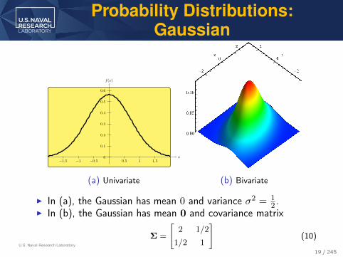
I Multivariate Gaussian distributions arise a lot: N{x;µ,Σ}:
N{z; z,R} = |2πR|− 12 e−
12
(z−z)′R−1(z−z). (9)
I Parameterized by mean vector µ and covariance matrix Σ.I Maximum entropy (most pessimistic) distribution when given
only µ and Σ.I Assuming noise is due to many small random contributions, a
justification for the Gaussian approximation is from the centrallimit theorem.(The sum of N independent and identically distributed random variablesapproaches a Gaussian distribution as N gets large).
I Noise in measurement domain typically approximated Gaussian.I Arises in certain areas with stochastic dynamic models.I Is a conjugate prior distribution.
18 / 245
U.S. Naval Research Laboratory
Probability Distributions:Gaussian
x
f(x)
−1.5 −1 −0.5 0.5 1 1.50
0.1
0.3
0.3
0.4
0.5
0.6
(a) Univariate (b) Bivariate
I In (a), the Gaussian has mean 0 and variance σ2 = 12 .
I In (b), the Gaussian has mean 0 and covariance matrix
Σ =
[2 1/2
1/2 1
](10)
19 / 245
U.S. Naval Research Laboratory
Probability Distributions:Chi-Squared
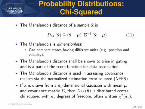
I The Mahalanobis distance of a sample x is
DM (x) , (x− µ)′Σ−1 (x− µ) (11)
I The Mahalanobis is dimensionless:I Can compare states having different units (e.g. position and
velocity).
I The Mahalanobis distance shall be shown to arise in gatingand is a part of the score function for data association.
I The Mahalanobis distance is used in assessing covariancerealism via the normalized estimation error squared (NEES).
I If x is drawn from a dx-dimensional Gaussian with mean µand covariance matrix Σ, then DM (x) is distributed centralchi squared with dx degrees of freedom, often written χ2(dx).
20 / 245

U.S. Naval Research Laboratory
Probability Distributions:Chi-Squared
x
f(x)
1 2 3 4 5 6 7 8 90
0.05
0.1
0.15
0.2
0.25
I The central chi-squared distribution with k degrees of freedomis
χ2(x, dx) =xk2−1e−
x2
2k2 Γ(k2
) (12)
where Γ is the gamma function.I Plotted is χ2(x, 3).I Confidence regions of a desired % are easily determined using
Gaussian approximations, Mahalanobis distances, andchi-squared statistics.
21 / 245

U.S. Naval Research Laboratory
Probability Distributions:Chi-Squared
I Given a Gaussian PDF estimate of a target, a point x, iswithin the first pth-percentile if
(x− µ)′Σ−1 (x− µ) < γp (13)
where γp depends on p and on dx, the dimensionality of x.
Confidence Region pdx 0.9 0.99 0.999 0.9999 0.999991 2.7055 6.6349 10.8276 15.1367 19.51142 4.6052 9.2103 13.8155 18.4207 23.02593 6.2514 11.3449 16.2662 21.1075 25.90176 10.6446 16.8119 22.4577 27.8563 33.10719 14.6837 21.6660 27.8772 33.7199 39.3407
Values of γp for p and dx.
I Use ChiSquareD.invCDF in the TCL to determine γp.22 / 245

U.S. Naval Research Laboratory
Probability Distributions:Chi-Squared
t1
t2
t3
t4m1m2
m3
m4
m6m5
m7
m8
I Uncertainty regions are ellipses/ellipsoids.I This type of test can be used for gating:
I Gating: Eliminating targets/measurements for considerationfor association to other targets/measurements.
I Gating reduces computational complexity of measurementassignment.
I Above example: t for targets (with confidence ellipses) and mfor measurements.
23 / 245
U.S. Naval Research Laboratory
Probability Distributions:Chi-Squared
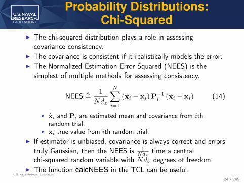
I The chi-squared distribution plays a role in assessingcovariance consistency.
I The covariance is consistent if it realistically models the error.I The Normalized Estimation Error Squared (NEES) is the
simplest of multiple methods for assessing consistency.
NEES ,1
Ndx
N∑
i=1
(xi − xi) P−1i (xi − xi) (14)
I xi and Pi are estimated mean and covariance from ithrandom trial.
I xi true value from ith random trial.I If estimator is unbiased, covariance is always correct and errors
truly Gaussian, then the NEES is 1Ndx
time a centralchi-squared random variable with Ndx degrees of freedom.
I The function calcNEES in the TCL can be useful.24 / 245
U.S. Naval Research Laboratory
Probability Distributions:Chi-Squared
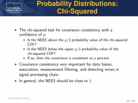
I The chi-squared test for covariance consistency with aconfidence of p:
I Is the NEES above the p/2 probability value of the chi-squaredCDF?
I Is the NEES below the upper p/2 probability value of thechi-squared CDF?
I If so, then the covariance is consistent to p percent.
I Covariance consistency very important for data fusion,association, measurement filtering, and detecting errors insignal processing chain.
I In general, the NEES should be close to 1.
25 / 245
U.S. Naval Research Laboratory
Probability Distributions:Binomial
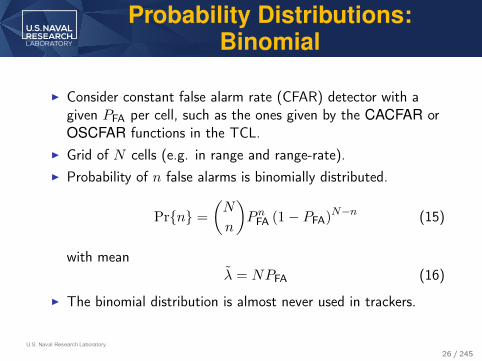
I Consider constant false alarm rate (CFAR) detector with agiven PFA per cell, such as the ones given by the CACFAR orOSCFAR functions in the TCL.
I Grid of N cells (e.g. in range and range-rate).I Probability of n false alarms is binomially distributed.
Pr{n} =
(N
n
)PnFA (1− PFA)N−n (15)
with meanλ = NPFA (16)
I The binomial distribution is almost never used in trackers.
26 / 245

U.S. Naval Research Laboratory
Probability Distributions:Binomial
I We fix the mean λ and vary N , which means that PFA mustchange:
PFA =λ
N(17)
I The probability of n false alarms becomes
Pr{n} =
(N
n
)λ
Nn
(1− λ
N
)N−n(18)
I What is limN→∞
Pr{n}?I First note that
limN→∞
(N
n
)λ
Nn= lim
N→∞Nn +O(Nn−1)
n!
λn
Nn=λn
n!(19)
I This leaves the term limN→∞
(1− λ
N
)N−n
27 / 245
U.S. Naval Research Laboratory
Probability Distributions:Binomial
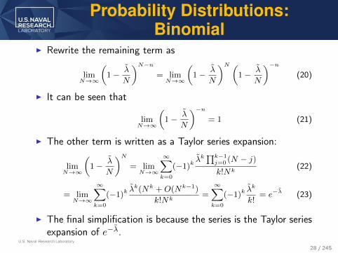
I Rewrite the remaining term as
limN→∞
(1− λ
N
)N−n= limN→∞
(1− λ
N
)N (1− λ
N
)−n(20)
I It can be seen that
limN→∞
(1− λ
N
)−n= 1 (21)
I The other term is written as a Taylor series expansion:
limN→∞
(1− λ
N
)N= limN→∞
∞∑k=0
(−1)kλk∏k−1j=0 (N − j)k!Nk
(22)
= limN→∞
∞∑k=0
(−1)kλk(Nk +O(Nk−1)
k!Nk=
∞∑k=0
(−1)kλk
k!= e−λ (23)
I The final simplification is because the series is the Taylor seriesexpansion of e−λ.
28 / 245

U.S. Naval Research Laboratory
Probability Distributions:Poisson
I The distribution resulting from holding λ constant and takingN →∞ is thus Poisson:
Pr{n} = e−λλn
n!(24)
I Typically one splits λ = λV .I λ is a false alarm density and V is a volume.
I For a range-range rate map, volume units might be m2/s2.
I Formulation of likelihood functions for target-measurementassociation simpler using Poisson approximation.
I Given λ, common likelihood formulations do not need to knowV .
29 / 245
U.S. Naval Research Laboratory
Probability Distributions:Poisson
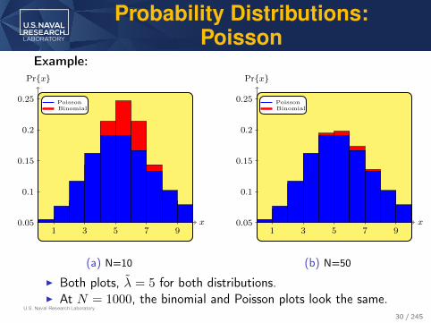
Example:
x
Pr{x}
1 3 5 7 90.05
0.1
0.15
0.2
0.25BinomialPoisson
(a) N=10
x
Pr{x}
1 3 5 7 90.05
0.1
0.15
0.2
0.25BinomialPoisson
(b) N=50
I Both plots, λ = 5 for both distributions.I At N = 1000, the binomial and Poisson plots look the same.
30 / 245

U.S. Naval Research Laboratory
Cubature Integration
I Many integrals cannot be solved analytically with a finitenumber of terms.
I Try to evaluate a Fresnel integral:
C(z) =
∫ z
0
cos
(πt2
2
)dt (25)
I Quadrature integration is a technique for efficient numericalevaluation of univariate integrals.
I Cubature integration is multivariate quadrature integration.I The TCL has many functions related to cubature integration
in “Mathematical Functions/Numerical Integration” and“Mathematical Functions/Numerical Integration/CubaturePoints.”
31 / 245

U.S. Naval Research Laboratory
Cubature Integration: Why?
Numerically integrate the function from 0 to 2.
x
f(x)
1 20
0.25
0.5
0.75
1
I Evaluate ∫ 2
0f(x) dx =? (26)
32 / 245

U.S. Naval Research Laboratory
Cubature Integration: Why?
Numerically integrate the function from 0 to 2.
x
f(x)
1 20
0.25
0.5
0.75
1
I Basic calculus solution: A Riemann sum:∫ 2
0f(x) dx ≈
N−1∑
k=0
f (k∆x) ∆x where 2 = N∆x. (27)
33 / 245

U.S. Naval Research Laboratory
Cubature Integration: Why?
I Riemann sums converge very slowly.I Finite precision errors for small ∆x add up fast.I Very inefficient in multiple dimensions.I Not always practicable for:
I Infinite integrals.I Integrals over weird shapes, such as a 4D hypersphere.
I Cubature integration produces exact solutions in someinstances.
I Matlab’s integral function uses adaptive quadrature.I One can do much better than Matlab’s function for certain
classes of integrals.
34 / 245

U.S. Naval Research Laboratory
Cubature Integration: Theory
I The idea in quadrature/cubature is the relation
∫
x∈Sf(x)w(x) dx =
N∑
i=0
ωif(xi), (28)
is exact for a particular weighting function w for allpolynomials f up to a certain order and approximate for otherfunctions f .
I S is a region, such as Rn or the surface of a hypersphere.I Unlike a Riemann sum, N is finite.I Cubature weights ωi and points xi depend on w and the order.
I Efficient: For a fifth-order integral with a multivariate Gaussianweighting function, one can choose points such that N = 12.
35 / 245
U.S. Naval Research Laboratory
Cubature Integration: Theory
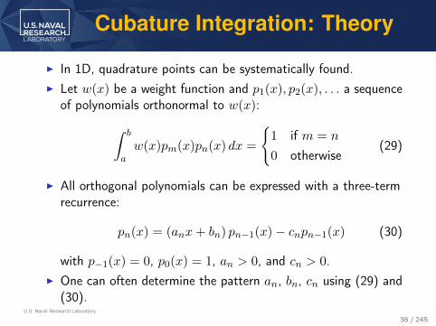
I In 1D, quadrature points can be systematically found.I Let w(x) be a weight function and p1(x), p2(x), . . . a sequence
of polynomials orthonormal to w(x):
∫ b
aw(x)pm(x)pn(x) dx =
{1 if m = n
0 otherwise(29)
I All orthogonal polynomials can be expressed with a three-termrecurrence:
pn(x) = (anx+ bn) pn−1(x)− cnpn−1(x) (30)
with p−1(x) = 0, p0(x) = 1, an > 0, and cn > 0.I One can often determine the pattern an, bn, cn using (29) and
(30).
36 / 245

U.S. Naval Research Laboratory
Cubature Integration: Theory
I The orthogonal polynomial pn(x) = kn∏ni=1(x− ti) with
kn > 0 has n distinct real roots (ti) between a and b.I It has been proven that knowing pn:
ωn = −(kN+1
kN
)1
pN+1(tn)pN (tn)n = 1, 2, . . . , N (31)
and the cubature points ξn = tn, where
pn(t) ,pn(x)
dx
∣∣∣∣x=t
(32)
I Efficient methods of solving the problem utilizing matrixdecompositions of the three-term recursion coefficients exist.
I 1D quadrature points can be extended into multipledimensions using either a Gaussian product method, or themethod of Smolyak (linCubPoints2MultiDim in the TCL).
I Specialized methods of generating cubature points also exist.37 / 245

U.S. Naval Research Laboratory
Cubature Integration
I For target tracking the most useful weighting function is
w(x) = N {x;µ,Σ} (33)
I Points typically tabulated for a N {0, I} distribution.I Transform to N {x;µ,Σ} as
ξn ← µ+ Σ12 ξn (34)
where Σ = Σ12
(Σ
12
)′(lower-triangular Cholesky
decomposition).
I Many formulae for cubature points are given inA. H. Stroud, Approximate Calculation of Multiple Integrals. Edgewood Cliffs, NJ: Prentice-Hall,Inc., 1971.
38 / 245

U.S. Naval Research Laboratory
On Solving Integrals
I Many parts of target tracking involve solving difficultmultivariate integrals.
I Many algorithms fall into one of two categories:1. Use cubature integral for the integrals.2. Use a Taylor series expansion to turn the problem polynomial
and solvable.
I This comes up again and again.
39 / 245

U.S. Naval Research Laboratory
The CRLB
I The Cramér-Rao Lower Bound (CRLB) is a lower bound onthe variance (or covariance matrix) of an unbiased estimator.
I Under certain conditions, the CRLB states
E{
(x−T(z)) (x−T(z))′}≥ J−1 (35)
I A matrix inequality refers to sorted eigenvalues.I x is the quantity being estimated.I T(z) is the best unbiased estimator.I J is the Fisher information matrix.I The expectation is taken over the conditional PDF p(z|x) if x
is deterministic.I The Fisher information matrix has two equivalent formulations:
JB =− E{∇x∇′x ln (p(z|x))
}(36)
= E{
(∇x ln (p(z|x))) (∇x ln (p(z|x)))′}
(37)
40 / 245

U.S. Naval Research Laboratory
Using the CRLB
I An estimator is deemed “statistically efficient” if its accuracyachieves the CRLB.
I Most tracking problems exactly or approximately satisfy theassumed regularity conditions.
I The CRLB is an important tool in assessing the performanceof an estimator.
I The CRLB can be used as an approximate measurementcovariance matrix.
I The square root of the trace of the position components of theCRLB can be used as a lower bound on the position root meansquared error (RMSE) when localizing a target.
I Many common track filters are very close to or achieve theCRLB in simple situations.
41 / 245

U.S. Naval Research Laboratory
Using the CRLB
I If x is not deterministic, take an expected value over x whencomputing the CRLB.
I Equivalent to computing the CRLB with expectations overp(x, z) instead of p(z|x).
I In instances where the CRLB cannot be achieved, a boundcalled the the Bhattacharya bound is tighter.
I In the TCL, functions related to the CRLB (and Fisherinformation matrix) are in “Dynamic Estimation/PerformancePrediction” as well as computePolyMeasFIM anddirectionOnlyStaticLocCRLB in “Static Estimation”, anddelayDopplerRateCRLBLFMApprox in “MathematicalFunctions/Signal Processing.”
I The proof of the multivariate CRLB is next, but is more forreference as it is long.
42 / 245
U.S. Naval Research Laboratory
The CRLB: Long Proof
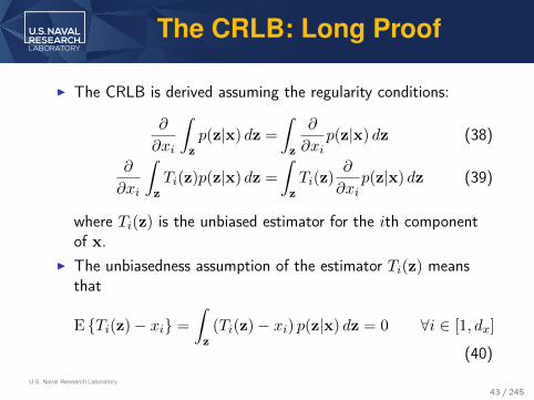
I The CRLB is derived assuming the regularity conditions:
∂
∂xi
∫
zp(z|x) dz =
∫
z
∂
∂xip(z|x) dz (38)
∂
∂xi
∫
zTi(z)p(z|x) dz =
∫
zTi(z)
∂
∂xip(z|x) dz (39)
where Ti(z) is the unbiased estimator for the ith componentof x.
I The unbiasedness assumption of the estimator Ti(z) meansthat
E {Ti(z)− xi} =
∫
z(Ti(z)− xi) p(z|x) dz = 0 ∀i ∈ [1, dx]
(40)
43 / 245

U.S. Naval Research Laboratory
The CRLB’s: Long Proof
I Differentiate both sides of the unbiasedness equation (usingregularity conditions) with respect to xi:
∫
z(Ti(z)− xi)
∂
∂xip(z|x) dz−
∫
zp(z|x) dz = 0 (41)
I Noting that a PDF integrates to 1:∫
z(Ti(z)− xi)
∂
∂xip(z|x) dz = 1 (42)
I We now construct a substitution. Note that
∂
∂xiln (p(z|x)) =
1
p(z|x)
∂
∂xip(z|x) (43)
so∂
∂xip(z|x) = p(z|x)
∂
∂xiln (p(z|x)) (44)
44 / 245

U.S. Naval Research Laboratory
The CRLB: Long Proof
I The substitution of the logarithm identity into the integral is∫
z(Ti(z)− xi) p(z|x)
∂
∂xiln (p(z|x)) dz = 1 (45)
I However, consider the following integral with xj for j 6= i:∫z
(Ti(z)− xi) p(z|x)∂
∂xjln (p(z|x)) dz =
∫z
(Ti(z)− xi)∂
∂xjp(z|x) dz
(46)
=∂
∂xj
∫z
Ti(z)p(z|x) dz− xi∫z
∂
∂xjp(z|x) dz (47)
=∂
∂xjxi = 0 (48)
45 / 245

U.S. Naval Research Laboratory
The CRLB: Long Proof
I Define the matrices:
Z =
T1(z)− x1
...Tdx(z)− xdx∂
∂x1p(z|x)
...∂
∂xdxp(z|x)
,
Y1
Y2
(49)
I The regularity conditions say that
E {Z} = 0 (50)
46 / 245

U.S. Naval Research Laboratory
The CRLB: Long Proof
I Given the regularity conditions:
Cov {Z} = E{ZZ′
}= E
{[Y1Y
′1 Y1Y
′2
Y2Y′1 Y2Y
′2
]}(51)
I Note that
E{Y1Y
′1
}= Cov {T(x)} (52)
E{Y1Y
′2
}=I (53)
E{Y2Y
′2
}=J (54)
where the identities with the logarithmic integrals led to (53)and J is the Fisher information matrix as given by
J = E{
(∇x ln (p(z|x))) (∇x ln (p(z|x)))′}
(55)
47 / 245

U.S. Naval Research Laboratory
The CRLB: Long Proof
I Simplifying
Cov {Z} =
[Cov {T(x)} I
I J
]≥ 0 (56)
where the inequality represents that the matrix has to bepositive (semi-)definite.
I Use a matrix identity related to the Schur complement:[A B
C D
][I 0
−D−1C
]=
[A−BD−1C B
0 D
](57)
with A = Cov {T(x)}, B = I, C = I, D = J to get Cov {Z}as the leftmost matrix in (57).
48 / 245

U.S. Naval Research Laboratory
The CRLB: Long Proof
I The matrix multiplying that is[
I 0
−D−1C I
]=
[I 0
−J−1 0
](58)
I It is known that the product of a positive semidefinite matrixand a positive definite matrix is positive semidefinite, so onecan write[A−BD−1C B
0 D
]=
[Cov {T(x)} − J−1 I
0 J
]≥ 0 (59)
I This finishes the proof that
Cov {T(x)} ≥ J−1 (60)
I The proof of the equivalence to an expectation of secondderivatives is omitted.
49 / 245

U.S. Naval Research Laboratory
The CRLB and the PCRLB
I The Posterior CRLB (PCRLB) is a recursive formulation of theCRLB that is well suited for assessing recursive discrete-timeestimation problems.
I A full proof of the PCRLB is given in:P. Tichavský, C. H. Muravchik, and A. Nehorai, “Posterior Cramér- Rao bounds for discrete-timenonlinear filtering,” IEEE Transactions on Signal Processing, vol. 46, no. 5, pp. 1386-1396, May1998.
I Here, we use the results for a system with linear dynamics andadditive noise of the form
xk =Fkxk−1 + vk (61)zk =h(xk) + wk (62)
where vk ∼ N {0,Qk} and wk ∼ N {0,Rk}.
50 / 245

U.S. Naval Research Laboratory
The CRLB and the PCRLB
I The Fisher information matrix at time k + 1 after ameasurement update is
Jk+1 = Q−1k −Q−1
k Fk
(Jk + F′kQ
−1k Fk
)−1F′kQ
−1k
+ E[(∇xk+1
hk+1(xk+1)′)R−1k+1
(∇xk+1
hk+1(xk+1)′)′]
(63)
I The expectation is evaluated over all possible simulationtracks, often via Monte Carlo simulation.
I The initial J0 can be set to the CRLB for the firstmeasurement.
I These expressions will be used later to evaluate estimatorperformance.
51 / 245

COORDINATE SYSTEMS
52 / 245

U.S. Naval Research Laboratory
Coordinate Systems:Classes of Coordinate Systems
1. Physical Coordinate SystemsI Temporal and spatial quantities linked to global physical observations.I Examples: WGS-84, GCRS, ITRS, UTC.
2. Semi-Physical Coordinate SystemsI Physical quantities linked to convenient mathematical models.I Examples: Latitude and longitude, geoid height, pressure altitude, UTM.
3. Purely MathematicalI Physical coordinate systems expressed in terms of mathematical.I Examples: Cartesian, spherical, ellipsoidal, r-u-v, polar.
4. Measurement Coordinate SystemsI Local mathematical systems linked to physical quantities.I Systems corrupted by refraction and other physical effects.
Overview on coordinate systems given in:D. F. Crouse, “An Overview of Major Terrestrial, Celestial, and Temporal Coordinate Systems for TargetTracking,” Formal Report, Naval Research Laboratory, no. NRL/FR/5344–16-10,279, 10 Aug. 2016,173 pages.
53 / 245

U.S. Naval Research Laboratory
Physical Coordinate Systems 1Ghost Ghost
Target
I Physical coordinate systems most important when usingmultiple sensors.
I Coordinate system establishment: “Sensor registration.”I Registration is not independent of measurement coordinate
system effects.I Poor registration/ignored measurement effects=Worse
estimates: “Ghosting” of targets.54 / 245

U.S. Naval Research Laboratory
Physical Coordinate Systems 2
Internationally highly bureaucratically standardized6
CSTGCommission on International
Coordination of Space Techniquesfor Geodesy and Geodynamics
IVSInternational VLBI Service
for Geodesy and Astrometry
IERSInternational Earth Rotation
and Reference Systems Service
IGSInternational GNSS Service
IAGInternational Association
of Geodesy
ILRSInternational LaserRanging Service
IDSInternational DORIS
Service
IUGGInternational Union of Geodesy
and Geophysics
ICSUInternational Council
for Science
IAUInternational Astronomical
Union
ICSU WDSICSU World Data System
COSPARCommittee on
Space Research
PSMSLPermanent Service
for Mean Sea Level
IGFSInternational Gravity
Field Service
BGIInternational Gravity
Bureau
ISGInternational Service
for the Geoid
ICETInternational Center
for Earth Tides
IDEMSInternational DEM
Service
ICGEMInternational Centre
for Global Earth Models
ITRF Centre ICRS CentreConventions CentreGGFC
Global GeophysicalFluids Centre
RS/PCRapid Service/
Predictions Centre
Earth OrientationCentre
SBOSpecial Bureau for
the Oceans
SBHSpecial Bureau for
Hydrology
SBASpecial Bureau for
the Atmosphere
Special Bureau forCombinations
AssociationMember Of
Has Commission Has Service Has Service Has Service
Has Service
Has Service
Established
MemberOf
Has Service Member Of
HasTechnique
Center
HasTechnique
Center
HasTechnique
Center
HasTechnique
Center
Member Of
Member Of
Member OfHas Service Has Service
Has ServiceHas Subcommission
Established
Established
MemberScientific Union
MemberScientific Union
Has Service
Has CentreHas CentreHas Centre Has Centre
Has Centre
Has BureauHas Bureau Has Bureau Has Bureau
IERS Product Centres
Fig. 3. A subset of the tangled web of international organizations behind many of the standards that form the basis of terrestrial and celestial coordinatesystems. The IERS is the primary organization in internationally standardizing celestial and terrestrial coordinate systems, which are described in its conventions[257]. The ICSU WDS is a multidisciplinary organization that supplanted the Federation of Astronomical and Geophysical Data Analysis Services (FAGS).The ISG used to be known as the International Geoid Service (IGeS). A number of professional organizations, such as the Institute of Navigation (ION),as well as many governmental organizations, including the NGA and the Naval Observatory in the United States, also play a role in establishing standardcoordinate systems.
either in the Cartesian location of networked sensors or in themeasurements of the sensors. That is, the algorithms do notexplicitly solve for the actual orientation of the sensor and aninitial estimate is necessary. For example, [61], [204], [324],and [371] all use linear approximations to deal with smallerrors in the range, elevation, and azimuth measurements ofmultiple sensors in three dimensions. However, these algo-rithms cannot be used for high-precision corrections if thelocal vertical at each of the sensors is biased, because, asillustrated in Fig. 2, the corrections for the bias cannot beexpressed as constant additive-or-multiplicative modificationsto the measured azimuthal angle.
The vertical bias problem is worse when considering algo-rithms such as [1], [247], [250], [370], and [372] that try toestablish a common 2D coordinate system among multiplesensors, as might be the case when using multiple radarsthat are incapable of making elevation measurements. If theradars are designed such that their local verticals align withthe local gravitational verticals, then the planes in which their
measurements are taken do not coincide and it is not possibleto establish a common 2D coordinate system among the radars.Over short distances, an ad-hoc 2D coordinate system can beestablished, but it will never be of high precision. On the otherhand, algorithms for aligning a 2D sensor with 3D sensorsdo exist [129], [131]. Though, the nonlinear bias estimationalgorithms of [133], [189] and the linearized algorithms of[130], [284], [321], which explicitly consider biases in the 3Dsensor orientation, all require initial orientation estimates.
In contrast, Section VIII of this report discusses how toperform sensor registration without an initial estimate using agravitational and a magnetic-field estimate. It also discusseshow the estimate can be refined using star measurements.Though the star-based orientation-estimation algorithm re-quires an initial estimate (or a brute-force search), citationsfor star-based orientation estimation with no prior informationare provided.
Whereas the majority of algorithms for sensor registrationfor tracking applications focus on the use of common obser-
55 / 245

U.S. Naval Research Laboratory
Physical Coordinate Systems 38
BCRSBarycentric Celestial
Reference System
TCBBarycentric Coordinate Time
(Temps Coordonnee Barycentrique)
ICRSInternational Celestial
Reference System
ICRFInternational Celestial
Reference Frame
HCRFHipparcos Celestial
Reference Frame
UCACU.S. Naval Observatory
CCD Astrograph Catalog
GCRSGeocentric CelestialReference System
TCGGeocentric Coordinate Time
(Temps Coordonnee Geocentrique)
GTRSGeocentric Terrestrial
Reference System
ITRSInternational Terrestrial
Reference System
ITRFInternational Terrestrial
Reference Frame
WGS 84World GeodeticSystem: 1984
TTTerrestrial Time
via TAI (or USNO Master Clock)
RealizedBy
RealizedBy
Realized By
RealizedBy
Realized Using
Realized Using
Displacement
ECEF
ECI
Rotation
Ideal Models
Ideal Models
Observation-Based References
Observation-Based References
Fig. 5. The base coordinate system for tracking in the solar system is the BCRS, which is the ICRS, which has no explicit time component, with TCBadded as time. The ICRS is realized using star catalogs as the ICRF in radio wavelengths and the HCRF in optical wavelengths. Alternatively, the UCACcan be used in place of the HCRF for more precise results. The pseudo-inertial reference frame for tracking near-Earth objects is the GCRS, which is a typeof ECI coordinate system. The GCRS is related to the BCRS by an affine transform, placing its origin at the center of the Earth and using a appropriatelyrelativistically scaled time scale, the TGB. The GTRS is a fixed-Earth model of which the common realization is the ITRS, whose definition is consistent withmany models of the past. The ITRS is realized through the ITRF, which is essentially the same as the current version of the WGS 84 standard, except forthe definition of the reference ellipsoid. Actual conversions between frames can be complicated and are generally performed with the aid of two intermediatereference frames, namely, the Celestial Intermediate Reference Frame (CIRS) and the Terrestrial Intermediate Reference System (TIRS) [257], [187, Ch. 9].ECEF coordinate systems are generally realized using a timescale other than TCG.
look as if they are placed on a faraway sphere (they are allaround). The alignment of the axes is defined with respect toa specific date (called an epoch). The reference epoch for theICRS is called J2000.0, which refers to noon (1200 hours)in terrestrial time (TT) on January 1st in the year 2000 inthe Gregorian calendar (the standard calendar used throughoutmost of the world today). Terrestrial time is shortly beforenoon time coordinated universal time (UTC) on that same date.
The orientation of the axes in the ICRS are nominally basedon the orientation of the mean equator and dynamical equinoxat the reference epoch. The x´ and y-axes are in the planeof the celestial equator with the x-axis (also known as theorigin of right ascension) pointing toward the dynamical vernalequinox at epoch.13 The z-axis is orthogonal to the plane ofthe celestial equator and points in a general northerly direction.The celestial equator is the projection of the Earth’s equatoronto the celestial sphere. The ecliptic is a circle projected onthe celestial sphere that coincides with the orbit of the Eartharound the Sun and is tilted roughly 23.4˝ from the celestialequator along the x-axis [285, Ch. 3.53]. The ecliptic is thesame as the apparent direction of the Sun in the sky as theEarth orbits the Sun. An equinox is when the ecliptic intersectsthe celestial equator. That is, the equinox occurs when the Sunappears to pass through these points in the sky. There are twoequinoxes each year. The vernal equinox occurs when the Sunappears to be going from South to North in the sky. In reality,the ecliptic is not a perfect circle and the equator of the Earth
13The symbol P, which also marks the x-axis in Fig. 4, represents thezodiacal constellation Aries. In ancient Greek times, the vernal equinoxpointed in the direction of Aries. Nowadays, it points toward the constellationAquarius due to precession (Precession is discussed in detail in AppendixE). A brief discussion on the history of the constellations and the zodiacalprecession is given in [280].
−92 −91.5 −91 −90.5 −90 −89.5 −893
3.5
4
4.5
5
5.5
6
Right Ascension (degrees)
Dec
lin
ati
on
(d
egre
es)
Fig. 6. The right ascension and declination in the ICRS of the stars nearBarnard’s star (in red) over a period of 80 years based on data in the Hipparcoscatalog (Barnard’s star is catalog entry 87937). One can see that Barnard’sstar has a large proper motion (the overlapping red circles), whereas theother stars barely move. The declination of the star is increasing as timeprogresses. The plot demonstrates how not all stars are poor for use asreference points in defining a non-rotating celestial coordinate system dueto their large motion over the years. The function iauPmsafe in the IAU’sStandards of Fundamental Astronomy (SOFA) library were used to change theepoch of the data. The points in red are at the epoch of the Hipparcos catalog(1994.25 TT), and 20 Julian years (a Julian year being precisely 365.25 days)prior and 20, 40, and 60 Julian years posterior to the epoch of the catalog.
wobbles with respect to the celestial sphere. Thus, the ICRS isnominally defined in terms of mean values of these quantities.
As noted in [353], practical systems align their axes basedon the locations of stars, so the precise definitions of the meanequator and dynamical equinox at epoch (which are compli-
I Most useful systems are Earth-centered Earth-fixed’ (foraircraft) and Earth-centered inertial (ECI) (for satellites).
I BCRS/ICRS best for tracking things far from EarthI For example, NASA and ESA’s Solar & Heliospheric
Observatory [SOHO] satellite.I ECEF and ECI via rigorously defined physical systems.I WGS-84 is used by the DoD and GPS.
56 / 245
U.S. Naval Research Laboratory
Physical Coordinate Systemsand the TCL
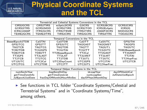
Terrestrial and Celestial Systems Conversions in the TCLCIRS2GCRS CIRS2TIRS ecliptic2ICRS G2ICRS GCRS2BCRS GCRS2CIRSGCRS2ITRS GCRS2MOD GCRS2TIRS GCRS2TOD ICRS2Ecliptic ICRS2GICRS2J2000F ITRS2GCRS ITRS2TEME ITRS2TIRS J2000F2ICRS MOD2GCRSTEME2GCRS TEME2ITRS TIRS2CIRS TIRS2GCRS TIRS2ITRS TOD2GCRS
Temporal Conversions in the TCLBesselEpoch2TDB Cal2TAI Cal2TDB Cal2TT Cal2UTC GPS2TAI
GPS2TCG GPS2TT GPS2UTC TAI2GAST TAI2GMST TAI2GPSTAI2TCB TAI2TCG TAI2TDB TAI2TT TAI2UT1 TAI2UTCTCB2TDB TCG2GPS TCG2TAI TCG2TT TCG2UTC TDB2BesselEpochTDB2TCB TDB2TT TT2BesselEpoch TT2Cal TT2GAST TT2GMSTTT2GPS TT2LAST TT2LAT TT2LMST TT2LMT TT2TAITT2TCB TT2TCG TT2TDB TT2UT1 TT2UTC TT2YearFracUT12UTC UTC2Cal UTC2DayCount UTC2GPS UTC2TAI UTC2TCBUTC2TCG UTC2TDB UTC2TT UTC2UT1 UTC2YearFrac
Temporal Helper Functions in the TCLnumSecInYear leapSecsOnDay isLeapYear dayOfWeek4Cal
getTimeZoneInfo getTimeZoneList cumLeapSec JulDate2JulEpochJulEpoch2JulDate fracDayOfMonth2HourMinSec dayOfYear2MonthDay
I See functions in TCL folder “Coordinate Systems/Celestial andTerrestrial Systems” and in “Coordinate Systems/Time”,among others.
57 / 245

U.S. Naval Research Laboratory
Semi-Physical CoordinateSystems I
ue
n
u
e
n
(a) ENU Axes
24
h
N
H
N
EllipsoidGeoidTerrain
Fig. 18. A grossly exaggerated representation of the deviations between thereference ellipsoid, the geoid, and the terrain. The arrows represent the localgravitational vertical on the reference geoid (MSL) as determined by gravity.The elevation of a marked point on the terrain above the reference ellipsoidis h (ellipsoidal height), which is calculated from a normal to the ellipsoid.Similarly, the geoid undulation N is the height of a point on the geoid abovethe reference ellipsoid traced out by a normal vector. On the other hand, theorthometric height H is the height that would be measured from the point tothe geoid by following the direction gradient from the point up or down untilit intersected the geoid. If the land were not there, it is the path that an idealplumb line would follow. The blue arrows coming of of the geoid representthe direction of the local vertical at those points. The distance N is often veryclose to N , so sometimes one approximates H « h ´ N .
tude coordinates with common commercial products, one mustbe aware that a number of companies base their coordinates ona warped, incorrect map projection. The Mercator projection isone of the most commonly used map projections because it isconformal, meaning that angles are locally preserved, thoughdistances are warped. However, many common online and mo-bile map applications use a warped Mercator projection calledthe “web Mercator projection” that was invented by Google,does not preserve angles, and on which latitude and longitudecoordinates usually do not correctly correspond to the WGS84 ellipsoidal coordinate system. The NGA has a presentationdetailing why the web Mercator projection produces maps thatare incompatible with the WGS 84 coordinate system, causingpositional biases to be as high as 40 km in some areas [242].
Additional details and derivations related to the geometry ofellipsoidal-Earth models are given in [270], [271], includinghow parameters for the reference ellipsoid are empiricallyfound from measurements.
V. VERTICAL HEIGHT AND GRAVITY
A. Definitions of Height
Whereas altitudes (heights) in the IERS conventions (whennot using a Cartesian coordinate system) are defined as h withrespect to the reference ellipsoid [257, Ch. 4.2.6], the WGS 84standard defines vertical datums with respect to the geoid. Thegeoid is a surface of constant gravitational potential definingMSL, or a local measure of MSL. An older version of theWGS-84 standard used to make an exception when describingthe depth of the ocean [69, Pgs. xii–xiv], where local soundingdatums were suggested, but the current version suggests thatall heights be reported at ellipsoidal heights [71, Ch. 10.6].
Figure 18 illustrates the differences between ellipsoidal andMSL (orthometric) elevations for a point on the surface ofthe Earth. The geoid is a hypothetical surface of constant
Height Type DescriptionAbsolute Altitude Distance from the center of the Earth
Height measured along the curved plumb lineOrthometric Height with respect to MSLAltitude based on a local pressure reading and aPressure Altitude standard atmospheric model
Geoid Height The distance between the reference ellipsoid andGeoid Undulation MSL (the geoid)Geodetic HeightEllipsoidal Height Height above the reference ellipsoid
Geopotential difference from surface, divided byGeopotential Height a standard acceleration magnitude g0TABLE VI
SOME OF THE MORE COMMON HEIGHT MEASURES THAT ARISE IN TARGETTRACKING PROBLEMS. IN MANY APPLICATIONS, ONLY APPROXIMATEVALUES OF ORTHOMETRIC HEIGHT AND GEOPOTENTIAL HEIGHT ARE
USED.
gravitational potential42 chosen to approximately coincide withthe height of the sea surface in the absence of tides (Onepossible definition of MSL. Note that multiple definitions ofMSL exist [78].). The distance between the geoid and thereference ellipsoid measured on a vertical from the referenceellipsoid is the geoid undulation N . The orthometric heightH of a point is the distance measured from that point to thegeoid by following the direction of gravity downward. This isthe usual definition of “height” when one describes the heightof a mountain, for example. The variable direction of gravityis referred to as the “curvature of the plumb line.” Thoughorthometric heights are defined in a manner related to howacceleration due to gravity changes as one moves, surfacesof constant orthometric height are not surfaces of constantgravity or gravitational potential. The ellipsoidal height h isapproximately the sum of the orthometric and geoidal heights.
Figure 19 plots the EGM2008 geoid with magnified undula-tions and the actual terrain according to the Earth2012 modelwith altitudes magnified with respect to MSL. Based solelyupon the distance from the center of the Earth, one mightexpect there to be no ocean near Europe based on the elevationin (b). However, since the geoid is high (red) near Europe, thelevel of the ocean by Europe is more distant from the centerof the Earth than the level of the ocean in the Caribbean.Orthometric height determines how high something seems interms of properties such as the thinness of the air. The air onthe top of Mount Everest (the highest mountain in the worldin terms of MSL) is thin because the top of Mount Everestis far above MSL. On the other hand, using the Earth2012terrain data, one finds that the most distant point from thecenter of the Earth is not Mount Everest, but rather is locatedin the northern Andes mountain range in South America.43
This is because the Earth is roughly ellipsoidal in shape, sopoints near the equator tend to be farther from the center ofthe Earth.
Table VI lists a number of different definitions ofheight/altitude that one might have to deal with when de-
42Contrary to what one might expect, the magnitude of acceleration dueto gravity is generally not constant on a surface of constant gravitationalpotential.
43The farthest point from the Earth’s center was the topic of the finalquestion in the 2013 National Geographic Bee with Chimborazo in Ecuadorbeing the most distant peak from the Earth’s center [15].
(b) Elevation and Geoid Height
I Ellipsoidal systems (latitude, longitude and altitude) as well asother maps (e.g. universal transverse mercator [UTM]).
I Local East-North-Up based on ideal ellipsoidal Earth.I Elevation on maps often measured with respect to geoid, not
reference ellipsoid.I Ellipsoid height h differs from exact (N +H) and approximate
(N +H) geoid (gravitational) height.58 / 245

U.S. Naval Research Laboratory
Semi-Physical CoordinateSystems II
(a) Exaggerated Earth Geoid
ï150 ï100 ï50 0 50 100 150
ï80
ï60
ï40
ï20
0
20
40
60
80
Magnetic Declination
Longitude
Latit
ude
degr
ees
ï150
ï100
ï50
0
50
100
150
(b) Magnetic Field v.s True North
I Geoid: Theoretical surface of constant gravitational potential.I Highest geoid height: Top of Mt. Everest (Himalayas).I Farthest point from Earth’s center: Top of Chimborazo
(Andes).I Magnetic coordinates considered semi-physical.
59 / 245

U.S. Naval Research Laboratory
Semi-Physical CoordinateSystems and the TCLMap-Related Functions in the TCL
ellips2Cart.m Cart2Ellipse getENUAxesgeogHeading2uVec uVec2GeogHeading uDotEllipsoid
proj2Ellips isInRefEllipsoid uDotNumeric
Gravity-Related Cooridinate Functions in the TCLMSL2EllipseHelmert ellips2MSLHelmert getEGMGeoidHeight
Magnetic-Related Conversions in the TCLCartCD2ITRS.m geogHeading2Mag ITRS2CartCD
ITRS2MagneticApex ITRS2QD magHeading2GeogspherCD2SpherITRS spherITRS2SpherCD trace2EarthMagApex
Pressure-Related Conversions in the TCLorthoAlt4Pres presTemp4OrthoAlt
I The above functions, and others, handle semi-physical systemsin the TCL.
60 / 245

U.S. Naval Research Laboratory
Mathematical CoordinateSystems
Common 3D Mathematical Systems: Monostatic r-u-v
x
y
z
r1
r1v
r 1u
I Monostatic range (one-way fromreceiver to the target) r1 and directioncosines u and v (z-axis points in radardirection)
x =r1u, (64)y =r1v, (65)
z =r1
√1− u2 − v2 (66)
I Direction cosines tend to work betterwith stochastic models than sphericalsystems.
I See Cart2Ruv, ruv2Cart and ruv2Ruv among others in theTCL.
61 / 245

U.S. Naval Research Laboratory
Mathematical CoordinateSystems
Common 3D Mathematical Systems: Bistatic r-u-v
x
y
z
r1
r1v
r 1u
lTx
r2
Tx
I Bistatic range rB = r1 + r2 anddirection cosines u and v.
x =r1u, (67)y =r1v, (68)
z =r1
√1− u2 − v2 (69)
r1 =r2B −
∥∥lTx∥∥2
2 (rB − u · lTx). (70)
I lTx is the transmitter location in thereceiver’s local coordinate system.
I A good system for the transmitterseparated from the receiver.
I See Cart2Ruv, ruv2Cart and ruv2Ruv among others in theTCL.
62 / 245
U.S. Naval Research Laboratory
Mathematical CoordinateSystems
Common Component: Range Rate
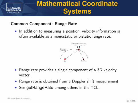
I In addition to measuring a position, velocity information isoften available as a monostatic or bistatic range rate.
Rx Tx/Rx
Bistaticvector
Monostaticvector
BistaticEllipse
I Range rate provides a single component of a 3D velocityvector.
I Range rate is obtained from a Doppler shift measurement.I See getRangeRate among others in the TCL.
63 / 245

U.S. Naval Research Laboratory
Mathematical CoordinateSystems
I With t indicating a 3X1 Cartesian position, the bistatic rangeis
rB =‖t− lRx‖+ ‖t− lTx‖ (71)
I Assuming Newtonian mechanics and no atmosphericrefraction, the range rate is a straightforward derivative ofrange with respect to time:
rB ,∂rB∂τ
=
(t− lRx + (t− lRx)τ
)′(t− lRx)
‖t− lRx + (t− lRx)τ‖+
(t− lTx + (t− lTx)τ
)′(t− lTx)
‖t− lTx + (t− lTx)τ‖(72)
rB |τ=0 =
(t− lRx
‖t− lRx‖ +t− lTx
‖t− lTx‖
)′t−
(t− lRx
‖t− lRx‖
)′lRx −
(t− lTx
‖t− lTx‖
)′lTx (73)
64 / 245

U.S. Naval Research Laboratory
Mathematical CoordinateSystems
Common 3D Mathematical Systems: Spherical
x
y
z
r1
λ Aφc, a
ζ
θϕ
I Multiple definitions (range, azimuth,elevation)
x = r1 cos(λ) cos(φc) (74)y = r1 sin(λ) cos(φc) (75)z = r1 sin(φc) (76)
or x = r1 sin(θ) cos(ϕ) (77)y = r1 sin(ϕ) (78)z = r1 cos(θ) cos(ϕ) (79)
among others.
I See Cart2Sphere and spher2Cart among others in the TCL.
65 / 245

U.S. Naval Research Laboratory
Mathematical CoordinateSystems: Rotations
z
y
zy
I Local versus global coordinate system rotations.I Textbooks devote many pages to transformations.I Simplified by using
S. Umeyama, “Least-squares estimation of transformation parameters between two pointpatterns,” IEEE Transactions on Pattern Analysis and Machine Intelligence, vol. 13, no. 4, pp.376-380, Apr. 1991.
I Given two unit vectors in each system, obtain rotation matrix.I Implemented as findTransParam in the TCL.I Similar findRFTransParam to orient radar face with respect to
reference ellipsoid.
66 / 245
U.S. Naval Research Laboratory
Mathematical CoordinateSystems and the TCL
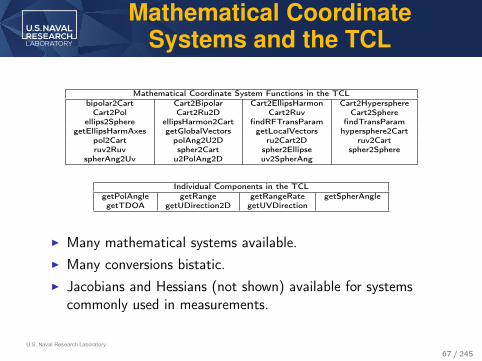
Mathematical Coordinate System Functions in the TCLbipolar2Cart Cart2Bipolar Cart2EllipsHarmon Cart2HypersphereCart2Pol Cart2Ru2D Cart2Ruv Cart2Sphere
ellips2Sphere ellipsHarmon2Cart findRFTransParam findTransParamgetEllipsHarmAxes getGlobalVectors getLocalVectors hypersphere2Cart
pol2Cart polAng2U2D ru2Cart2D ruv2Cartruv2Ruv spher2Cart spher2Ellipse spher2Sphere
spherAng2Uv u2PolAng2D uv2SpherAng
Individual Components in the TCLgetPolAngle getRange getRangeRate getSpherAnglegetTDOA getUDirection2D getUVDirection
I Many mathematical systems available.I Many conversions bistatic.I Jacobians and Hessians (not shown) available for systems
commonly used in measurements.
67 / 245

U.S. Naval Research Laboratory
Measurement CoordinateSystems
65.5 66 66.5 67
−1.4
−1.2
−1
−0.8
−0.6
−0.4
−0.2
0
0.2
0.4
Degrees East of North
Deg
rees
Ele
vati
on
Sunrise near Hilo Hawaii, 1 June 2013.Standard refraction makes the sun over thehorizon (red) while physically below thehorizon (blue). Use readJPLEphem to readephemeris data in the TCL.
I Measurements are corrupted from geometric quantities byphysical effects: Atmospheric refraction, general relativity, etc.
I Example: “Stationary” receivers move ±15 cm during day dueto solid-Earth tides.
I The GPS literature is a good source of very detailed physicalperturbations.
I The TCL has a number of standard monostatic/bistaticrefraction corrections in “Atmospheric Models/StandardExponential Model.”
68 / 245

MEASUREMENTS AND NOISE
69 / 245

U.S. Naval Research Laboratory
Measurements and Noise
x
y
I Are these points false alarms or a possible track over time?I Are they accurate measurements that are far apart?I Are false alarms very unlikely or highly likely?
70 / 245

U.S. Naval Research Laboratory
Measurements and Noise
x
y
I Are these points false alarms or a possible track over time?I These are the same points as before at a different scale.I Measurements are inherently noisy.I Knowledge of measurement noise level determines scale.
71 / 245

U.S. Naval Research Laboratory
Measurements and Noise
x
y
I The blue line is “connect-the-dots.” The orange line just addsinterpolation.
I The blue/orange lines are only good if the points are veryaccurate.
I The green line is much more reasonable if the points areinaccurate.
I The noise level determines the best fit.72 / 245

U.S. Naval Research Laboratory
Measurements and Noise
I Information on measurement accuracy is important forI Discerning false alarms from tracks.I Estimating a target state more accurately than “connecting the
dots”.
I The noisy nature of the measurements necessitates the use ofstatistics to accurately estimate a target state.
I The noise is often approximated as additive zero-meanmultivariate Gaussian in the local coordinate system of themeasurement. For a measurement z the true value z is thusdistributed
N{z; z,R} = |2πR|− 12 e−
12
(z−z)′R−1(z−z). (80)
where R is the covariance matrix of the measurement.
73 / 245
U.S. Naval Research Laboratory
Measurements and Noise:Circular Statistics
θ
f(θ)
240◦ 300◦ 60◦ 120◦
This weightgot clipped!
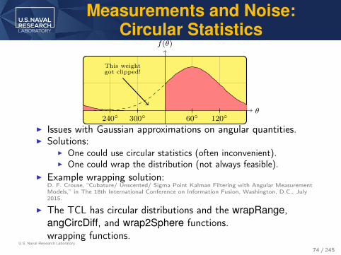
I Issues with Gaussian approximations on angular quantities.I Solutions:
I One could use circular statistics (often inconvenient).I One could wrap the distribution (not always feasible).
I Example wrapping solution:D. F. Crouse, “Cubature/ Unscented/ Sigma Point Kalman Filtering with Angular MeasurementModels,” in The 18th International Conference on Information Fusion, Washington, D.C., July2015.
I The TCL has circular distributions and the wrapRange,angCircDiff, and wrap2Sphere functions.wrapping functions.
74 / 245

U.S. Naval Research Laboratory
Measurements and Noise:Signal Processing
I Designers of tracking algorithms should be familiar with somesignal processing because:
I Detection algorithm designers seldom derive a covariance R(or other statistics) for their algorithms.
I When R is given, it is often lacking cross terms (e.g. betweenrange and range rate) even when the waveform leads to a truecoupling.
I Range and/or range-rate ambiguity can sometimes be solveddirectly in a multihypothesis tracker (MHT).
I Understanding the measurement signal processing informsabout when zero mean/Gaussian approximations beak down.
75 / 245

U.S. Naval Research Laboratory
Measurements and Noise:Cross Correlations
-4 -3 -2 -1 0 1 2 3Doppler Rate (1/microseconds)
-25
-20
-15
-10
-5
0
5
10
15
20
25
Del
ay (m
icro
seco
nds)
Ambiguity Function (dB)
-60
-50
-40
-30
-20
-10
0
I The wideband ambiguity function for a 2MHz linearlyfrequency modulated (LFM) chip lasting 20, µs
I Detections will most likely be on the ridge.I Errors in range → errors in range rate (Doppler) along the
ridge → correlations between range and range-ratemeasurement components.
76 / 245

U.S. Naval Research Laboratory
Measurements and Noise:Directional Estimation
Limits of Common Assumptions: Directional Estimation
0 5 10 15 20 25 30
Sum-Beam SNR, dB
0
0.1
0.2
0.3
0.4
0.5
0.6
0.7
0.8
RM
SE
RMSE via CRLB
ML Estimator
Quasi-Mean Estimator
Amplitude-Conditioned Mean Estimator
Prony Estimator
0 5 10 15 20 25 30
Sigmal Amplitude, dB
-0.05
0
0.05
0.1
0.15
0.2
0.25
0.3
0.35
0.4
0.45
Off
set
of
Est
imato
r M
ean
vs.
Tru
th
ML Estimator
Quasi-Mean Estimator
Amplitude-Conditioned Mean Estimator
Prony Estimator
I Rule of thumb for linear arrays: For direction cosine estimatesbelow 13 dB signal to noise ratio (SNR), “biases” arise,measurement distribution decreasingly Gaussian, varianceestimators from the Cramér-Rao Lower Bound (CRLB) arepoor.
77 / 245

U.S. Naval Research Laboratory
Measurements and Noise:Directional Estimation
I A statistically unbiased estimator of x given z is the expectedvalue E {x |z}.
I Suppose that one observes many independent trials z1, . . . , zn,so n is large and the true value of x is xtrue
I One usually expects that
limn→∞
1
n
n∑
i=1
E {x |zi } → E {x |z1, . . . , zn } = xtrue (81)
I That is not always true.I Counterexample:
I A linear array produces estimates of u ∈ (−1, 1).I If the true value is at or near −1, noise will always make
E {x |zi } > −1 unless the distribution is a delta function at −1I The mean of n→∞ numbers that are all > −1 will be > −1.
78 / 245

U.S. Naval Research Laboratory
Measurements and Noise:Directional Estimation
I Though E {x |zi } is unbiased in the strict statistical sense, itcan be “biased” in how one expects it to function.
I Algorithms utilizing Gaussian approximations implicitly assumethat that the average of multiple independent estimatesapproaches the true value.
I Directional estimates with low SNR and/or that are near theedges of the valid estimation region violate commonapproximations.
I Gaussian approximations ignoring such effects might work untilthe revisit rate becomes very fast.
I Estimator’s predicted error (via covariance matrix)approaches/ goes below magnitude of the “bias”.
79 / 245

U.S. Naval Research Laboratory
Measurements and Noise:Directional Estimation
I Understanding the limits of the signal processing origins ofmeasurements allows one to choose more appropriate targettracking methods.
I Traditional methods, such as the Kalman filter, becomeunreliable.
I More sophisticated/ computationally-demanding techniques,such as particle filters, might become necessary.
80 / 245

MEASUREMENT CONVERSION
81 / 245

U.S. Naval Research Laboratory
Measurement Conversion
I Cartesian conversion of noisy measurements is sometimesnecessary.
I Gaussian measurement will be non-Gaussian in Cartesiancoordinates.
I Given the measurement function z = h(t) over the range of zand the distribution of z is p(z) then the exact PDF of theconverted measurement is
pconv(t) = |J|−1 p(h(t)) (82)
J , (∇zt′)′
=(∇zh
−1(z)′)′
=(
(∇th(t)′)′)−1
(83)
I ∇z denotes the gradient operator. J is the Jacobian matrix.I For example, between r − u− v and Cartesian coordinates
J =
[∂
∂rt,∂
∂ut,∂
∂vt
](84)
82 / 245

U.S. Naval Research Laboratory
Measurement Conversion
-6000 -4000 -2000 0 2000 4000 6000y
-60
-40
-20
0
20
40
60
z
0
0.5
1
1.5
10-9
(a) PDF in Cartesian Coordinates
-6000 -4000 -2000 0 2000 4000 6000y
-60
-40
-20
0
20
40
60
z
0
0.5
1
1.5
10-9
(b) Gaussian Approximation
I Example, The monostatic r-u-v to Cartesian conversion.I PDF and Gaussian approximation in (a) and (b).
I Gaussian approximation matches first two moments.I Offsets are with respect to mean PDF value.I R = diag
([10, 10−3, 10−3
])and ztrue = [0, 0, 200× 103].
83 / 245

U.S. Naval Research Laboratory
Measurement Conversion
I For a bijective measurement function z = h(zCart),zCart = h−1(z) and additive Gaussian noise, the true meanzCart and covariance matrix RCart of a measurement zmeasconverted to Cartesian coordinates is:
E{
h−1(z)∣∣ zmeas
}= zCart =
∫z∈Rdz
h−1(z)N {z; zmeas,R} dz (85)
E{(
h−1(z)− zCart) (
h−1(z)− zCart)′∣∣∣ zmeas
}= RCart =∫
z∈Rdz
(h−1(z)− zCart
) (h−1(z)− zCart
)′N {z; zmeas,R} dz (86)
I Both integrals can be approximated using cubature integration.I See “Coordinate Systems/Conversions with
Covariances/Cubature Conversions” and AtmosphericModels/Standard Exponential Model/Cubature Conversions’ inthe TCL.
84 / 245

U.S. Naval Research Laboratory
Measurement ConversionI Cubature-based measurement conversion is the most versatile.
I Cross-correlation terms are trivially taken into account byincluding them in R.
I Non-additive Gaussian noise can be handled by replacingh−1(z) with h−1(z,w).
I h could include ray-traced atmospheric refractive effects.I An alternative approach in the literature is based on Taylor
series expansions.I See “Coordinate Systems/Conversions with
Covariances/Taylor-Series Conversions” in the TCL.I Given the model
z = h(zCart)−w (87)I Invert the equation
zCart = h−1 (z + w) (88)
I A Taylor series expansion about w = 0 is
zCart = h−1 (z) +(∇zh
−1 (z)′)′
w + . . . (89)85 / 245

U.S. Naval Research Laboratory
Measurement Conversion
I Given the Taylor series expansion, some approaches in theliterature truncate it at first order and use the expected valueand covariance:
zCart = E{
h−1 (z) +(∇zh
−1 (z)′)′
w}
=h−1 (z) (90)
RCart = E{(∇zh
−1 (z)′)′
ww′(∇zh
−1 (z)′)}
(91)
I For example, for polar measurements (r, θ):
zCart =
[r cos(θ)
r sin(θ)
](92)
RCart =
[σ2r cos(θ)
2 − 2rσrθ cos(θ) sin(θ) + r2σ2θ sin(θ)
2(σ
2r − r
2σ2θ) cos(θ) sin(θ) + rσrθ cos(2θ)
(σ2r − r
2σ2θ) cos(θ) sin(θ) + rσrθ cos(2θ) σ
2r sin(θ)
2+ r cos(θ)(rσ
2θ cos(θ) + 2σrθ sin(θ))
](93)
86 / 245
U.S. Naval Research Laboratory
Measurement Conversion
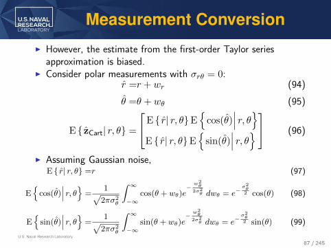
I However, the estimate from the first-order Taylor seriesapproximation is biased.
I Consider polar measurements with σrθ = 0:r =r + wr (94)
θ =θ + wθ (95)
E { zCart| r, θ} =
E { r| r, θ}E{
cos(θ)∣∣∣ r, θ
}
E { r| r, θ}E{
sin(θ)∣∣∣ r, θ
}
(96)
I Assuming Gaussian noise,E { r| r, θ} =r (97)
E{
cos(θ)∣∣∣ r, θ} =
1√2πσ2
θ
∫ ∞−∞
cos(θ + wθ)e− w2
θ2σ2θ dwθ = e−
σ2θ2 cos(θ) (98)
E{
sin(θ)∣∣∣ r, θ} =
1√2πσ2
θ
∫ ∞−∞
sin(θ + wθ)e− w2
θ2σ2θ dwθ = e−
σ2θ2 sin(θ) (99)
87 / 245
U.S. Naval Research Laboratory
Measurement Conversion
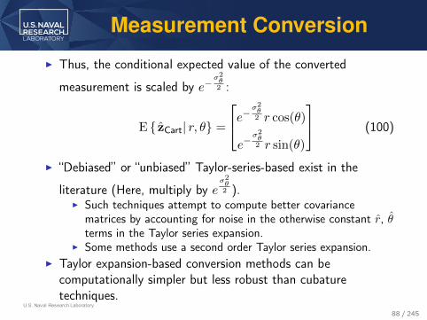
I Thus, the conditional expected value of the converted
measurement is scaled by e−σ2θ2 :
E { zCart| r, θ} =
e−σ
2θ2 r cos(θ)
e−σ2θ2 r sin(θ)
(100)
I “Debiased” or “unbiased” Taylor-series-based exist in the
literature (Here, multiply by eσ2θ2 ).
I Such techniques attempt to compute better covariancematrices by accounting for noise in the otherwise constant r, θterms in the Taylor series expansion.
I Some methods use a second order Taylor series expansion.I Taylor expansion-based conversion methods can be
computationally simpler but less robust than cubaturetechniques.
88 / 245

U.S. Naval Research Laboratory
Measurement ConversionExample I
50 100 150 200 250 300 350 4000
500
1000
1500
2000
2500
3000
3500
4000
4500
Round−Trip Monostatic Range [km]
RM
SE
[m
ete
rs]
CRLB
Simplex UKF Points
CKF Points
CM2
4th Order UKF Points
5th Order Cubature Points
(a) RMSE
50 100 150 200 250 300 350 4000
0.5
1
1.5
2
2.5
Round−Trip Monostatic Range [km]
NE
ES
Simplex UKF Points
CKF Points
CM2
4th Order UKF Points
5th Order Cubature Points
(b) NEES
I Monostatic r − u− v to Cartesian measurement conversionwith the target at u = 0 and v = sin (45◦); range varied.
I Black NEES lines are the 95% confidence region.I R = diag([10m, 10−2, 10−2])2
I CM2 is a second-order Taylor-series expansion method, simplexUKF=second order cubature, CKF= third-order cubature.
89 / 245

U.S. Naval Research Laboratory
Measurement ConversionExample II
50 100 150 200 250 300 350 4000
500
1000
1500
2000
2500
3000
3500
4000
4500
Bistatic Range Beyond the Baseline [km]
RM
SE
[m
ete
rs]
CRLB
Simplex UKF Points
CKF Points
4th Order UKF Points
5th Order Cubature Points
(a) RMSE
50 100 150 200 250 300 350 4000
0.5
1
1.5
2
2.5
Bistatic Range Beyond the Baseline [km]
NE
ES
Simplex UKF Points
CKF Points
4th Order UKF Points
5th Order Cubature Points
(b) NEES
I An example of bistatic r − u− v to Cartesian measurementconversion with the transmitter at (20 km, 20 km, 20 km) andtarget and noise parameters as in monostatic case.
I The difference in algorithms is most obvious in the NEES.
90 / 245

BAYES’ THEOREM AND THE LINEARKALMAN FILTER UPDATE
91 / 245

U.S. Naval Research Laboratory
Bayes’ Theorem
I Given a PDF p(x) representing the target state estimate at aparticular time.
I Given a measurement z and a conditional PDF of themeasurement p(z|x).
I Bayes’ theorem states thatposterior
distribution︷ ︸︸ ︷p(x|z) =
measurementdistribution︷ ︸︸ ︷p(z|x)
priordistribution︷︸︸︷p(x)
p(z)︸︷︷︸normalizing constant
(101)
I The value p(z) is essentially a normalizing constant.
p(z) =
∫
x∈Sp(z|x)p(x) dx (102)
where S is whatever space x is in (For discrete variables, theintegral becomes a sum).
92 / 245

U.S. Naval Research Laboratory
Bayes’ Theorem: Monte HallExample
I Bayes’ theorem underlies all rigorous measurement updatealgorithms in tracking.
I A simple example of Bayes theorem is the Monte Hall problem:
I You are given a choice of three doors. Behind one door is a carand goats are behind the other two. You pick a door and thehost opens a different door behind which there is a goat. Whatare your odds of finding a car if you stay with the originallychosen door versus picking the other remaining door?
93 / 245

U.S. Naval Research Laboratory
Bayes’ Theorem: Monte HallExample
I x is the door behind which there is a car. The initial set ofprobabilities p(x) for each door is uniform:
d1 d2 d3p(x) 1/3 1/3 1/3
I Without loss of generality, assume you choose door 1. Themeasurement likelihood function p(z|x) is:
x d1 d2 d31 0 1/2 1/22 0 0 13 0 1 0
I Without loss of generality, assume that the host opens doornumber 2. Applying Bayes’ theorem one gets p(x|z) to be
d1 d2 d3p(x|z) 1/3 0 2/3
I The best choice is to switch doors.I Most people think it doesn’t matter. Bayes’ theorem can
outperform one’s instincts.
94 / 245
U.S. Naval Research Laboratory
Bayes’ Theorem and JointDistributions
I Suppose the joint distribution p(x, z) is known.I Using the definition of conditional probability
p(x, z) = p(z|x)p(x) (103)
I This allows Bayes’ theorem to be rewritten
p(x|z) =p(z|x)p(x)
p(z)=p(x, z)
p(z)(104)
95 / 245

U.S. Naval Research Laboratory
Bayes’ Theorem and JointGaussian Distirbutions
I Assume that the state x and measurement z are jointlyGaussian.
p(x, z) = N{
y︷︸︸︷[x
z
];
y︷ ︸︸ ︷[xprior
zprior
],
Pyy︷ ︸︸ ︷[Pprior Pxz
prior
Pzxprior Pzz
prior
]}(105)
I Using Bayes’ rule for the update one gets
p(x|z) =p(x, z)
p(z)(106)
=|Pyy|− 1
2 e−12
(y−y)′Pyy(y−y)
∣∣∣Pzzprior
∣∣∣− 1
2e−
12
(z−zprior)′Pzzprior(z−zprior)(107)
96 / 245

U.S. Naval Research Laboratory
Bayes’ Theorem: LinearGaussian Distributions
I After considerable simplification, one finds that the posteriorp(x|z) is Gaussian with mean and covariance matrix
xposterior =xprior + Pxzprior
(Pzz
prior)−1
(z− zprior) (108)
Pposterior =Pprior −Pxzprior
(Pzz
prior)−1
Pzxprior (109)
I The joint Gaussian assumption holds for the linear Gaussianmodel p(x) ∼ N {xprior,Pprior} and
z = Hx + w (110)
where w ∼ N {0,R}.I The conditional measurement distribution is Gaussianp(z|x) ∼ N {Hx,R}.
I Note thatzprior = E {z} = E {Hx} = Hxprior (111)
I It can be shown that p(z) ∼ N {zprior,Pzz}.97 / 245
U.S. Naval Research Laboratory
Bayes’ Theorem: LinearGaussian Distributions
I The covariance terms are
Pzzprior = E
{(z− zprior)(z− zprior)
′}
=R + HPpriorH′ (112)
Pxzprior = E
{(x− xprior)(z− zprior)
′}
=PpriorH′ (113)
I Substituting everything back for the linear model one gets theupdate step for the Kalman filter.
I Notation change for standard tracking:I The “prior” subscript will be replaced by “k|k − 1” to indicate
that one has an estimate of a current (step k) state given prior(step k − 1) information.
I The “posterior” subscript will be replaced by “k|k” to indicatethat one has an estimate of a current state given currentinformation.
98 / 245

U.S. Naval Research Laboratory
Bayes’ Theorem: LinearGaussian DistributionsPrior Predictionxk|k−1,Pk|k−1
Measurementzk,Rk
Measurement Predictionzk|k−1 = Hkxk|k−1
Innovationνk = zk − zk|k−1
Innovation CovariancePzz
k|k−1 = Rk +HkPk|k−1H′k
Cross CovariancePxz
k|k−1 = Pk|k−1H′k
Filter Gain
Wk = Pxzk|k−1
(Pzz
k|k−1
)−1
Updated CovariancePk|k = (I−WkHk) (I−WkHk)
′+WkRkW
′k
Updated State Estimatexk|k = xk|k−1 +Wkνk
I The discrete measurement update step of the Kalman filterwith common notation/terminology.
I The updated covariance estimate has been reformulated inJoseph’s form for numerical stability.
I See KalmanUpdate in “Dynamic Estimation/MeasurementUpdate” in the TCL.
99 / 245

U.S. Naval Research Laboratory
Bayes’ Theorem: Joseph’sForm
I One would expect the covariance update to be
Pk|k = Pk|k−1 −Wk
(Pxzk|k−1
)′(114)
I However, finite precision errors can possibly cause the Pk|k tohave a negative eigenvalue even if Pk|k−1 is positive definite.
I The subtraction is the problem.I Solution: Replace the subtraction with a quadratic expression.I The quadratic expression
Pk|k = (I−WkHk) (I−WkHk)′ + WkRkW
′k (115)
is algebraically equivalent to (114) and does not suffer a risk ofnegative eigenvalues.
100 / 245

U.S. Naval Research Laboratory
Bayes’ Theorem: Why UseApproximations?
I The Kalman filter update is optimal for measurements that arelinear combinations of the target state.
I One approach to handling nonlinear measurements (i.e.anything from a radar) for a Cartesian state is the previouslydiscusses measurement conversion and Gaussianapproximation.
I However, why not just apply Bayes’ theorem more precisely?I Bayes’ theorem is again:
p(x|z) =p(z|x)p(x)
p(z)(116)
I Just multiply two known functions and normalize the result.
I Bayes’ theorem is trivial. Why not always do it optimally?
101 / 245

U.S. Naval Research Laboratory
Bayes’ Theorem: Why UseApproximations?
I The Gaussian distribution is a conjugate prior distribution toitself.
I If p(x) is Gaussian and p(z|x) is Gaussian, then p(x|z) mustbe Gaussian.
I See “Mathematical Functions/Statistics/Conjugate PriorUpdates.”
I Some other examples of conjugate prior distributions are:x p(x) p(z|x)
λ Poisson gammaPFA binomial betaσ2 scalar normal inverse gammaΣ multivariate normal inverse Wishart
I If the measurement distribution is not conjugate to the priordistribution, the result of Bayes’ rule will be increasinglycomplicated.
I Not suitable for recursive estimation.102 / 245

U.S. Naval Research Laboratory
Bayes’ Theorem: Why UseApproximations?
I Bayes’ theorem is just normalized multiplication. Why not justdiscretize space and do everything almost optimally on a grid?
I Simplest “optimal” Bayesian filter:1. Discretize the entire estimation space2. Evaluate probabilities on a discrete grid for given distributions3. Multiply matrices of probabilities to get posterior; normalize
I It is simple.I With parallelization over GPUs, couldn’t it be done quickly?
103 / 245

U.S. Naval Research Laboratory
Bayes’ Theorem: Why UseApproximations?
I Why the brute-force grid approach is seldom done:I One target 3D position and velocity in 50 km cube all directions about
sensor, speed in any direction to Mach 4 (1372,m/s), discretized to 5mand 1m/s.
I Grid for single probability density function (PDF) is more than 2× 10²²
in size (we need two).I As floating doubles, one grid requires more than 82 zettabytes of RAM
(1 ZB=1 trillion GB).I 64GB RAM stick ≈ $255 so cost ≈ $330 trillion ($660 trillion for two
grids, US GDP ≈ $53 trillion).I Computing power to multiply two grids in 1ms is ≈ 20 exaflops.I Most powerful supercomputer (Tianhe-2, China) 33.85 petaflops. We
need 612 of them.I A smarter approach would be to use some type of adaptive grid or set of
points.I This is the basis of particle filters (to be discussed later).
I The Kalman filter is much faster than the most efficient particle filter.104 / 245

U.S. Naval Research Laboratory
Bayes’ Theorem: Can’t itAlways be Linear?
I Why not always make the state in the local coordinate systemof the receiver?
I For example, [r, u, v, r, u, v] instead of position and velocity.I The linear Kalman filter measurement update is optimal for
additive Gaussian measurement noise.I This approach is widely used in the open literature for missile
control systems.I The use of range rate becomes much simpler.I Drawbacks:
I There is no common “local” coordinate system for multiplesensors/multiple measurement types. E.g. monostatic plusbistatic measurements.
I Non-maneuvering targets follow curved trajectories in localcoordinates.
I Nonlinear dynamic models are more difficult to handle thannonlinear measurements.
105 / 245

U.S. Naval Research Laboratory
Bayes’ Theorem: Can’t itAlways be Linear?
I Consider a 2D position vector r in a polar coordinate system:
ur =
[cos(θ)
sin(θ)
]uθ =
∂ur∂θ
=
[− sin(θ)
cos(θ)
](117)
r =rur (118)I Note that
ur =∂ur∂θ
θ = θuθ uθ =− θur (119)
I The velocity isr =rur + rur = rur + rθuθ (120)
I Thus, the acceleration isr =rur + rur + rθuθ + rθuθ + rθuθ =
(r − rθ2
)︸ ︷︷ ︸
ar
ur +(rθ + 2rθ
)︸ ︷︷ ︸
aθ
uθ (121)
I For constant ar = 0 and aθ = 0, one gets the nonlineardynamic model:
r =rθ2 θ =− 2rθ
r(122)
106 / 245
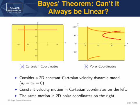
U.S. Naval Research Laboratory
Bayes’ Theorem: Can’t itAlways be Linear?
r
θ
−30 15 15 30
−40
20
0
20
40
(a) Cartesian Coordinates
r
θ
18 27 36 45
−90◦
0◦
90◦
180◦
(b) Polar Coordinates
I Consider a 2D constant Cartesian velocity dynamic model(ar = aθ = 0).
I Constant velocity motion in Cartesian coordinates on the left.I The same motion in 2D polar coordinates on the right.
107 / 245
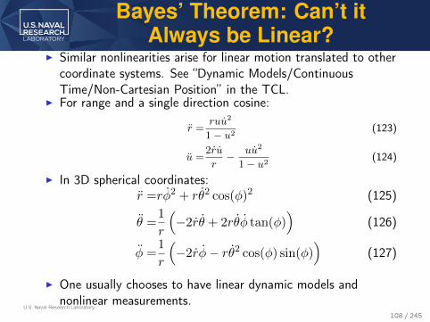
U.S. Naval Research Laboratory
Bayes’ Theorem: Can’t itAlways be Linear?
I Similar nonlinearities arise for linear motion translated to othercoordinate systems. See “Dynamic Models/ContinuousTime/Non-Cartesian Position” in the TCL.
I For range and a single direction cosine:
r =ruu2
1− u2(123)
u =2ru
r− uu2
1− u2(124)
I In 3D spherical coordinates:r =rφ2 + rθ2 cos(φ)2 (125)
θ =1
r
(−2rθ + 2rθφ tan(φ)
)(126)
φ =1
r
(−2rφ− rθ2 cos(φ) sin(φ)
)(127)
I One usually chooses to have linear dynamic models andnonlinear measurements.
108 / 245

STOCHASTIC CALCULUS AND LINEARDYNAMIC MODELS
109 / 245

U.S. Naval Research Laboratory
Stochastic Calculus:Motivation
I A physicist providing a sophisticated dynamic model (ballistic/orbital, spiraling, weaving, turning, etc), will probably initiallycreate a deterministic differential equation:
dxtdt
=
What PhysicsTells You︷ ︸︸ ︷a(xt, t) (128)
I . . . but objects under track are not deterministic.I Physics offers an approach: A stochastic differential equation:
dxt =
What PhysicsTells You︷ ︸︸ ︷
a(xt, t)dt +
UnknownPerturbations︷ ︸︸ ︷D(xt, t)dβt (129)
I a(xt, t) is the drift function.I D(xt, t) is the diffusion matrix.I dβt is the differential of a Wiener process.
110 / 245

U.S. Naval Research Laboratory
Stochastic Calculus: Details
I Instead of using the notation
dxt = a(xt, t)dt+ D(xt, t)dβt (130)
one typically wants to write a traditional differential equation:
dxtdt
= a(xt, t) + D(xt, t)dβtdt
(131)
I For practical purposes, (130) is equivalent to (131).I . . . but under strict mathematical definitions, dβtdt does not
exist.I However integrals over the term are defined.
111 / 245

U.S. Naval Research Laboratory
Stochastic Calculus: Details
I The evolution of the Wiener process vectorβt = [βt(1), βt(2), . . . , βt(dw)]′ is defined as
p(βt2 − βt1) =1√
2π(t2 − t1)exp
[−(βt2 − βt1)2
2(t2 − t1)
](132)
β0 =0 (133)E [βt2 |βt1 ] =βt1 (134)
E [βt] =0 (135)
I This property is important for deriving explicit solutions tocertain systems.
I However, one must first define what a stochastic integral is.
112 / 245

U.S. Naval Research Laboratory
Stochastic Calculus: Details
I In Calculus II, definite integrals of real functions are oftenderived related to Riemann sums:
∫ b
af(t)dt , lim
N→∞
N−1∑
j=0
f(τj) (tj+1 − tj) (136)
witht0 =a tj =t0 + ∆tj ∆t =
b− aN
(137)
I τj ∈ [tj , tj+1] and it generally does not matter where.I The more esoteric Riemann-Stieltjes integral adds in another
function g(t) as a measure:∫ b
af(t)dg(t) , lim
N→∞
N−1∑
j=0
f(τj) (g(tj+1)− g(tj)) (138)
I Again τj ∈ [tj , tj+1] and it generally does not matter where.113 / 245

U.S. Naval Research Laboratory
Stochastic Calculus: Details
I The strict definition of the Riemann-Stieltjes integral is notsuited to measures g(t) that vary infinitely in a given interval.
I A Wiener process βt varies infinitely in a given interval, butthe definition of the integral used is similar to aRiemann-Stieltjes integral:
∫ b
af(t)dβt = lim
N→∞
N−1∑
j=0
f(τj)(βtj+1 − βtj
)(139)
I Unlike with Riemman and Riemann-Stieltjes integrals,choosing different values of τj ∈ [tj , tj+1] changes the results.
I Choosing τj = tj results in Itô calculus.I Choosing τj =
tj+1+tj2 results in Stratonovich calculus.
I Itô calculus is simpler and is usually the only one used.
114 / 245

U.S. Naval Research Laboratory
Stochastic Calculus: DetailsI Given a definition of a calculus, an integral over a stochastic
differential equation takes a form akin to a Riemann sum:
xb = limN→∞
N−1∑
j=0
(a(xτj , τj)∆
t + D(xτj , τj
) (βtj+1
− βtj))
(140)
I The integral result is random, because βtj is random.I However, the intermediate values of xτj are required.I One can consider the integral over an infinitesimal step:
xt+∆t = xt + a(xτ , τ)∆t + D (xτ , τ)(βt+∆t − βt
)(141)
which is akin to Euler’s method for deterministic differentialequations.
I Stochastic Runge-Kutta methods and other techniques existfor better solutions to stochastic differential equations. SeeStrongStochRungeKStep and WeakStochRungeKStep inthe TCL.
115 / 245

U.S. Naval Research Laboratory
Stochastic Calculus: LinearSystems
I For linear systems, explicit solutions are available.I For linear systems, Itô and Stratonovich calculus are the same.
I The calculi only differ if D(xt, t) depends on xt.
I Consider the linear difference equation:
dxt = Axtdt+ Bdβt (142)
where A and B are constant matrices.I The integral of the stochastic differential equation from t0 to t
is
xt = xt0 +
∫ t
t0
Axτdτ +
∫ t
t0
Bdβτ (143)
where the second integral is stochastic.
116 / 245

U.S. Naval Research Laboratory
Stochastic Calculus: LinearSystems
I Rather than directly solve the integral, we note that theinfinitesimal step
xt+∆t = xt + Axt∆t + B
(βt+∆t − βt
)(144)
is Gaussian distributed if xt is deterministic of Gaussiandistributed. Thus, the solution to the entire integral isGaussian distributed.
I As (144) is linear, the solution to the integral must have theform
xt = Ft−t0xt0 + v (145)
where v ∼ N {0,Qt−t0} and w is the same dimensionality asβt.
I Ft−t0 and Qt−t0 must be determined.
117 / 245

U.S. Naval Research Laboratory
Stochastic Calculus: LinearSystems
I A second infinitesimal step has the form
xt+2∆t =xt+∆t + Axt+∆t∆t + B(βt+2∆t − βt+∆t
)(146)
=
Same as two steps for dxtdt
= Axt︷ ︸︸ ︷xt + 2Axt∆
t + A2xt(∆t)2
+(I + ∆tA
)B(βt+∆t − βt
)+ B
(βt+2∆t − βt+∆t
)(147)
I F thus comes from integrating the non-stochastic differentialequation
dxtdt
= Axt (148)
given xt0 .I This differential equation is solved in the control literature.
118 / 245

U.S. Naval Research Laboratory
Stochastic Calculus: LinearSystems
I The integral that must be solved the determine F is∫ t
t0
Axtdt (149)
I The solution utilizes a property of the exponential function ofa matrix.
d
dteAt = AeAt = eAtA (150)
I The exponential of a matrix is defined as a generalization ofthe Taylor series expansion of eλt:
eAt ,∞∑
k=0
1
k!tkAk (151)
119 / 245

U.S. Naval Research Laboratory
Stochastic Calculus: LinearSystems
I The differential equation to solve is
xt = Axt (152)
I Pre and post multiply by e−At
e−Atxt − e−AtAxt = 0 (153)
I Utilizing the property of the matrix exponential
d
dt
(e−Atxt
)= 0 (154)
I Integrating from t0 to t yields
xt = eA(t−t0)xt0 (155)
so Ft−t0 = eA(t−t0).120 / 245

U.S. Naval Research Laboratory
Stochastic Calculus: LinearSystems
I We must determine the process noise covariance matrix Q tofinish finding the posterior distribution.
I We propose that the solution to the stochastic differentialequation dxt = Axtdt+ Bdβt is
xt = Ft
(xt0 +
∫ t
t0
Ddβτ
)(156)
I It can be shown that if t = t0, then xt = xt0 , satisfying theinitial conditions.
I Differentiating (156), one gets
dxt =dFt−t0dt
(xt0 +
∫ t
t0
Ddβτ
)+ Ft−t0Ddβt (157)
I The proof by induction comes from substituting (157) intoxt = x0 +
∫ tt0dxτdτ and simplifying to get
xt = xt0 +∫ tt0
Axτdτ +∫ tt0
Bdβτ again.121 / 245

U.S. Naval Research Laboratory
Stochastic Calculus: LinearSystems
I From the definition of differences of βt and theRiemann-Stieltjes-like definition of the stochastic integral, oneknows that ∫ t
t0
dβτ ∼ N {0, (t− t0)I} (158)
I Given the proposed solution, the covariance of the predictioncan be found to be
Qt−t0 = E{
(xt − Ft−t0xt0) (xt − Ft−t0xt0)′∣∣xt0
}(159)
I The integral is over matrix exponentials (Ft−t0 is a matrixexponential). The solution is the linDynMod2Disc function inthe TCL and the algorithm is fromC. F. Van Loan, "Computing Integrals Involving the Matrix Exponential," IEEE Transactions onAutomatic Control, vol. AC-23, no. 3, pp. 395-404, Jun. 1967.
I We now have the tools to convert linear continuous-timemodels to linear discrete-time models.
122 / 245
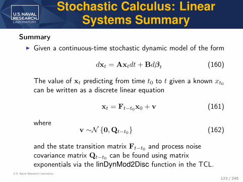
U.S. Naval Research Laboratory
Stochastic Calculus: LinearSystems Summary
SummaryI Given a continuous-time stochastic dynamic model of the form
dxt = Axtdt+ Bdβt (160)
The value of xt predicting from time t0 to t given a known xt0can be written as a discrete linear equation
xt = Ft−t0x0 + v (161)
wherev ∼N {0,Qt−t0} (162)
and the state transition matrix Ft−t0 and process noisecovariance matrix Qt−t0 can be found using matrixexponentials via the linDynMod2Disc function in the TCL.
123 / 245

U.S. Naval Research Laboratory
Stochastic Calculus: LinearDynamic Models
The following classes of linear dynamic models shall be discussed:1. The family of nearly constant moment models (velocity,
acceleration, jerk, etc.).I See FPolyKal and QPolyKal in the TCL.
2. The family of correlated nearly constant moment models(Ornstein-Uhlenbeck, Singer, etc.).
I See FGaussMarkov and QGaussMarkov in the TCL.
124 / 245

U.S. Naval Research Laboratory
Stochastic Calculus: LinearDynamic Models
I The nearly constant velocity model (continuous white noiseacceleration model) in 1D is
dxt︷︸︸︷[xt
xt
]=
A︷ ︸︸ ︷[0 1
0 0
]xtdt+
B︷︸︸︷[0
q
]dβt (163)
I Noise is only added to the velocity term.I q is the process noise intensity. Typical units are
√m2/s3.
I The state transition and process noise covariance matrices forpredicting T , t− t0 are
F =
[1 T
0 1
]Q =
1
3T 3 1
2T 2
1
2T 2 T
q2 (164)
125 / 245

U.S. Naval Research Laboratory
Stochastic Calculus: LinearDynamic Models
I The nearly constant acceleration model in 1D is similarly
dxt =
0 1 0
0 0 1
0 0 0
xtdt+
0
0
q
dβt (165)
I Noise is only added to the acceleration term.I The state transition and process noise covariance matrices for
predicting T ahead are (omitting subscripts of F and Q):
F =
1 T1
2T 2
0 1 T
0 0 1
Q =
1
20T 5 1
8T 4 1
6T 3
1
8T 4 1
3T 3 1
2T 2
1
6T 3 1
2T 2 T
q2 (166)
126 / 245

U.S. Naval Research Laboratory
Stochastic Calculus: LinearDynamic Models
I The pattern can be generalized to where the nth derivativehas the noise added:
A =
0 for n = 0 (the scalar case)[0n,1 In,n
0 01,n
]for n > 0
(167)
D =
[0n,1
1
]q (168)
I The values in row r and column c (starting from 0) of thetransition matrix and process noise covariance matrix topredict ahead T are:
Fr,c =
T c−r
(c− r)! if c− r ≥ 0
0 otherwise(169)
Qr,c =T (n−r)+(n−c)+1
(n− r)!(n− c)!((n− r) + (n− c) + 1)q2 (170)
127 / 245

U.S. Naval Research Laboratory
Stochastic Calculus: LinearDynamic Models
I 1D motion models can be generalized to d dimensions as Fd
and Q|d via a Kronecker product:
Fd =
Id,dF0,0 Id,dF0,1 . . . Id,dF0,n
Id,dF1,0 Id,dF1,1 . . . Id,dF1,n
......
. . ....
Id,dFn,0 Id,dFn,1 . . . Id,dFn,n
(171)
Qd =
Id,dQ0,0 Id,dQ0,1 . . . Id,dQ0,n
Id,dQ1,0 Id,dQ1,1 . . . Id,dQ1,n
......
. . ....
Id,dQn,0 Id,dQn,1 . . . Id,dQn,n
(172)
where Idd is a d× d identity matrix.I In Matlab, use Fd=kron(F,eye(d,d)).
128 / 245
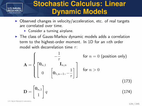
U.S. Naval Research Laboratory
Stochastic Calculus: LinearDynamic Models
I Observed changes in velocity/acceleration, etc. of real targetsare correlated over time.
I Consider a turning airplane.I The class of Gauss-Markov dynamic models adds a correlation
term to the highest-order moment. In 1D for an nth ordermodel with decorrelation time τ :
A =
−1
τfor n = 0 (position only)
0n,1 In,n
0
[01,n−1,−
1
τ
] for n > 0
(173)
D =
[0n,1
1
]q (174)
129 / 245

U.S. Naval Research Laboratory
Stochastic Calculus: LinearDynamic Models
I The elements of the state transition matrix and the processnoise covariance matrix for the discretized Gauss-Markovmodel are:
Fr,c =
T c−r
(c− r)! if r≤c and c<n
(−τ)n−r(e−
Tτ −
n−r−1∑i=0
(−Tτ
)ii!
)if c = n
0 otherwise
(175)
Qr,c =q2(−τ)2n−r−c+1n−r−1∑i=0
(−1)i(
1− e−Tτ
i∑k=0
(Tτ
)kk!
)
+ q2(−τ)2n−r−c+1n−c−1∑i=0
(−1)i(
1− e−Tτ
i∑k=0
(Tτ
)kk!
)
− q2 1
2(−τ)2n−r−c+1
(1− e−2T
τ
)+ q2(−τ)2n−r−c
n−r−1∑i=0
n−c−1∑j=0
(−1)i+jT(Tτ
)i+ji!j!(i+ j + 1)
(176)
130 / 245
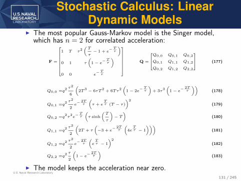
U.S. Naval Research Laboratory
Stochastic Calculus: LinearDynamic Models
I The most popular Gauss-Markov model is the Singer model,which has n = 2 for correlated acceleration:
F =
1 T τ2(T
τ− 1 + e
−Tτ
)
0 1 τ
(1− e−
Tτ
)
0 0 e−Tτ
Q =
Q0,0 Q0,1 Q0,2
Q0,1 Q1,1 Q1,2
Q0,2 Q1,2 Q2,2
(177)
Q0,0 =q2 τ
2
6
(2T
3 − 6τT2+ 6Tτ
2(1− 2e
−Tτ
)+ 3τ
3(1− e−
2Tτ
))(178)
Q0,1 =q2 τ
2
2e− 2Tτ
(τ + e
Tτ (T − τ)
)2(179)
Q0,2 =q2τ2e−Tτ
(τ sinh
(T
τ
)− T
)(180)
Q1,1 =q2 τ
2
2
(2T + τ
(−3 + e
− 2Tτ
(4eTτ − 1
)))(181)
Q1,2 =q2 τ
2
2e− 2Tτ
(eTτ − 1
)2(182)
Q2,2 =q2 τ
2
(1− e−
2Tτ
)(183)
I The model keeps the acceleration near zero.131 / 245
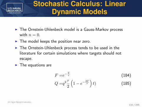
U.S. Naval Research Laboratory
Stochastic Calculus: LinearDynamic Models
I The Ornstein-Uhlenbeck model is a Gauss-Markov processwith n = 0.
I The model keeps the position near zero.I The Ornstein-Uhlenbeck process tends to be used in the
literature for certain simulations where targets should notescape.
I The equations are
F =e−Tτ (184)
Q =q2 τ
2
(1− e− 2T
τ
)t) (185)
132 / 245

U.S. Naval Research Laboratory
Stochastic Calculus vs. DirectDiscrete Models
I Direct discrete-time models exist and do not require stochasticcalculus.
I One example is the discrete white-noise acceleration model. In1D with discrete time k:
xk+1 =Fxk + Γv (186)
F =
[1 T
0 1
]Γ =
1
2T 2
T
(187)
I The term v is scalar noise with variance q2.I The term Γ treats the noise as inputs to velocity and
acceleration terms in a simple scalar kinematic model
x = xT +1
2xT 2 (188)
133 / 245

U.S. Naval Research Laboratory
Stochastic Calculus: ProcessNoise
I The power spectral density term q2 of the process noise is adesign parameter.
I If one typically predicts over a duration of T and the maximumchange in the highest order moment of your state (e.g.velocity, acceleration, etc) is vMAX, a rule-of-thumb for mostdiscretized dynamic models is
q2 ≈(
34vMAX
)2
T(189)
I Multiple other rules of thumb exist (including for directdiscrete models) and are programmed into theprocessNoiseSuggest function in the TCL.
134 / 245

U.S. Naval Research Laboratory
Stochastic Calculus vs. DirectDiscrete Models
I Though simple to derive, direct discrete models should usuallybe avoided:
I Predictions are temporally inconsistent when used with varyingrevisit rates T .
I This is explained in more detail when considering the Kalmanfilter prediction.
I The process noise covariance matrix is singular, which cansometimes cause issues.
I Functions for some linear direct discrete models in the TCLinclude FVanKeuk. QPolyKalDirectDisc, QPolyKalDirectAltand QVanKeuk.
135 / 245

THE LINEAR KALMAN FILTERPREDICTION
136 / 245

U.S. Naval Research Laboratory
The Linear Kalman FilterPrediction
I The stochastic dynamic models describe prediction when theinitial state x is deterministic.
I What if the initial state is uncertain?I Assume a Gaussian prior at discrete step k − 1 with mean
xk−1|k−1 and covariance matrix Pk−1|k−1.I The goal is to predict forward to discrete step k, resulting in a
predicted distribution with mean and covariance matrix xk|k−1
and covariance matrix Pk|k−1.I The discretized or discrete dynamic model
xk = Fk−1xk−1 + wk−1 (190)
where the subscript of F refers to the discrete time, not theduration of the prediction and wk−1 ∼ N {0,Qk−1}.
I Fk−1 and Qk−1 can be for any linear model; they depend onthe prediction interval T .
137 / 245
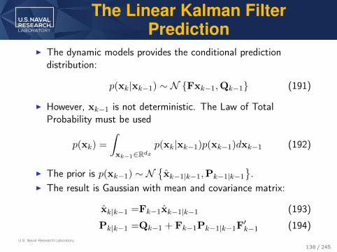
U.S. Naval Research Laboratory
The Linear Kalman FilterPrediction
I The dynamic models provides the conditional predictiondistribution:
p(xk|xk−1) ∼ N {Fxk−1,Qk−1} (191)
I However, xk−1 is not deterministic. The Law of TotalProbability must be used
p(xk) =
∫
xk−1∈Rdxp(xk|xk−1)p(xk−1)dxk−1 (192)
I The prior is p(xk−1) ∼ N{xk−1|k−1,Pk−1|k−1
}.
I The result is Gaussian with mean and covariance matrix:
xk|k−1 =Fk−1xk−1|k−1 (193)
Pk|k−1 =Qk−1 + Fk−1Pk−1|k−1F′k−1 (194)
138 / 245

U.S. Naval Research Laboratory
The Linear Kalman FilterPrediction Summary
Prior Valuesxk−1|k−1,Pk−1|k−1
State Predictionxk|k−1 = Fkxk−1|k−1
Covariance PredictionPk|k−1 = Qk + FkPk|k−1F′k
I The final two equations are the prediction step of the standardKalman filter.
I See the discKalPred function in the TCL.I We now have tools to approximate measurements as Gaussian,
predict states forward and update states with convertedmeasurements.
139 / 245

U.S. Naval Research Laboratory
Discretized Versus DirectDiscrete and the Kalman Filter
I Consider two scenarios:I Predicting a target state forward by T using the Kalman filter
and then predicting it forward by another T .I Predicting a target state forward by 2T .
I The results of both predictions should be the same.I If using a discretized dynamic model, they are the same.I If using a direct discrete model, they are not the same.I Direct discrete models are problematic with possibly missed
detection and variable revisit rates.
140 / 245

LINEAR INITIAL STATE ESTIMATION ANDTHE INFORMATION FILTER
141 / 245
U.S. Naval Research Laboratory
Linear Initial State Estimation
Two common approaches to starting the filter are1. One-point initiation.
I See the functions in “Dynamic Models/One-PointInitialization” in the TCL.
2. Using an information filter.I See infoFilterUpdate and infoFilterDiscPred in the TCL.
142 / 245
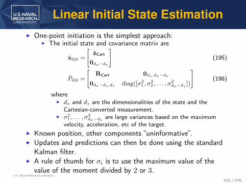
U.S. Naval Research Laboratory
Linear Initial State EstimationI One-point initiation is the simplest approach:
I The initial state and covariance matrix are
x0|0 =
[zCart
0dx−dz
](195)
P0|0 =
[RCart 0dz ,dx−dz
0dx−dz ,dz diag([σ21 , σ
22 , . . . , σ
2dx−dz ])
](196)
whereI dx and dz are the dimensionalities of the state and the
Cartesian-converted measurement.I σ2
1 , . . . , σ2dx−dz are large variances based on the maximum
velocity, acceleration, etc of the target.I Known position, other components “uninformative”.I Updates and predictions can then be done using the standard
Kalman filter.I A rule of thumb for σi is to use the maximum value of the
value of the moment divided by 2 or 3.143 / 245
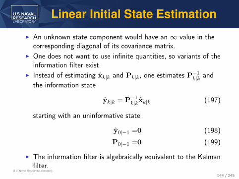
U.S. Naval Research Laboratory
Linear Initial State Estimation
I An unknown state component would have an ∞ value in thecorresponding diagonal of its covariance matrix.
I One does not want to use infinite quantities, so variants of theinformation filter exist.
I Instead of estimating xk|k and Pk|k, one estimates P−1k|k and
the information state
yk|k = P−1k|kxk|k (197)
starting with an uninformative state
y0|−1 =0 (198)
P0|−1 =0 (199)
I The information filter is algebraically equivalent to the Kalmanfilter.
144 / 245

U.S. Naval Research Laboratory
Linear Initial State Estimation
Information State Updateyk|k = yk|k−1 +H′kR
−1k zk
State Information UpdateP−1
k|k = P−1k|k−1
+H′kR−1k Hk
Information State Predictionyk|k−1 = Dk−1yk−1|k−1
State Prediction Information MatrixP−1
k|k−1= Dk−1P
−1k−1|k−1
F−1k−1
Dk−1 =(F′k−1 +P−1
k−1|k−1F−1
k−1Qk−1
)−1
Information State at Time k − 1yk−1|k−1
State Information Matrix at Time k − 1
P−1k−1|k−1
I Multiple variants of the information filter exist; one is shownabove, combining prediction and update steps.
I Once enough measurements for state observability have beenfiltered, one can recover the state:
xk|k = Pk|kyk|k (200)
145 / 245

NONLINEAR MEASUREMENT UPDATES
146 / 245

U.S. Naval Research Laboratory
Nonlinear MeasurementUpdatesSingle Model
Estimation AlgorithmsBatch
Estimation
RecursiveEstimationGaussian Filters Particle Filters
Maximum LikelihoodAlgorithms
Particle Filters
StochasticParticle Filters
DeterministicParticle Filters
GaussianMixture Filters
No BiasCompensation
BiasCompensation
Consider ExtendedKalman Filter
Consider CubatureKalman Filter
Extended Kalman FilterCubature Kalman FilterPure Propagation Filter
Progressive Gaussian Filter
Quasi-Monte Carlo Filter
Ensemble Kalman FilterCentral Difference Kalman FilterDivided Difference Kalman Filter
Bootstrap PF
Auxiliary PF
PF with Kalman Filter Proposal
Box PFInstrument Variable PF
Homotopy PF
I Measurement updates are possible without Cartesian conversion.I Major nonlinear filtering algorithms shown.I We focus on the Extended Kalman Filter and variants of the cubature
Kalman filter (which include the “unscented” KF).I See EKFUpdate and cubKalUpdate in the TCL.
147 / 245

U.S. Naval Research Laboratory
Nonlinear MeasurementUpdates
I The Kalman filter arose from a Bayesian update given that alinear measurement and the state are jointly Gaussian.
I Approximating a nonlinear measurement
z = h(x) + w (201)
where w is Gaussian, as jointly Gaussian with the state, onestill has the same basic update equations as the Kalman filter
xk|k =xk|k−1 + Pxzk|k−1
(Pzzk|k−1
)−1 (z− zk|k−1
)(202)
P|k =Pk|k−1 −Pxzk|k−1
(Pzzk|k−1
)−1Pzxk|k−1 (203)
but the quantities zk|k−1, Pzzk|k−1, Pxz
k|k−1 are now integrals.
148 / 245

U.S. Naval Research Laboratory
Nonlinear MeasurementUpdates
The integrals are:
zk|k−1 = E [h(xk) + wk] (204)
=
∫Rdx
h(xk)N{xk; xk|k−1,Pk|k−1
}dxk (205)
Pzzk|k−1 = E
[(zk − zk|k−1
) (zk − zk|k−1
)′] (206)
= E[(
wk+h(xk)−zk|k−1
)(wk+h(xk)−zk|k−1
)′] (207)
=Rk +
∫Rdx
(h(xk)− zk|k−1
) (h(xk)− zk|k−1
)′N{xk; xk|k−1,Pk|k−1
}dxk
(208)
Pxzk|k−1 = E
[(xk − xk|k−1
) (zk − zk|k−1
)′] (209)
= E[(
xk − xk|k−1
)(h(xk) + wk − zk|k−1
)′] (210)
=
∫Rdx
(xk − xk|k−1
) (h(xk) + zk|k−1
)′N{xk; xk|k−1,Pk|k−1
}dxk
(211)
149 / 245

U.S. Naval Research Laboratory
Nonlinear MeasurementUpdates: CKF
Predicted Estimatesxk|k−1
Pk|k−1
Measurement Predictionzk|k−1 =
∑Nci=1 ωiz
(i)p
Innovationνk = zk − zk|k−1
Updated State Estimatexk|k = xk|k−1 + Wkνk
Predicted Cubature State Points
x(i)p = xk|k−1 + P
12k|k−1
ξi
Predicted Cubature Measurement Pointsz(i)p = h
(x(i)p
)
Filter Gain
Wk = Pxzk|k−1
(Pzz
k|k−1
)−1
Updated State CovariancePk|k =
(Xp −WkZp
)(Xp −WkZp
)′+ WkRkW
′k
Base Cubature Points and WeightsChoose dx-dimensional cubature points {ξi} and weights
{ωi}.
Centered, Predicted Cubature Point MatrixXp=
[√ω1(x
(1)p −xk|k−1), . . . ,
√ωNc (x
(Nc)p −xk|k−1)
]
Centered, Predicted Cubature Measurement Point MatrixZp=
[√ω1(z
(1)p −zk|k−1), . . . ,
√ωNc (z
(Nc)p −zk|k−1)
]
Innovation CovariancePzz
k|k−1 = Rk + ZpZ′p
Cross CovariancePxz
k|k−1 = XpZ′p
Measurementzk,Rk
I The simplest solution to the nonlinear integrals is to usecubature integration, shown above.
I The square root is a lower-triangular Cholesky decomposition.I The vector formulation above requires all cubature weights be
positive, but allows for Joseph’s form to be used.I A Joseph’s formulation supporting negative cubature weights
is probably impossible.150 / 245

U.S. Naval Research Laboratory
Nonlinear MeasurementUpdates: EKF
I The Quasi Monte-Carlo Kalman filter is the same as the CKF,but uses Monte Carlo integration for the integrals.
I An alternative approach is to use a Taylor series expansion ofthe nonlinear function.
I A first-order Taylor series expansion of h(xk) about the pointxk|k−1 is:
h (xk) ≈ h(xk|k−1
)+(∇xh
(xk|k−1
)′)′ (xk − xk|k−1
)(212)
I The expected values are thus:
zk|k−1 =h(xk|k−1
)(213)
Hk =(∇xh
(xk|k−1
)′)′ (214)
Pzzk|k−1 =Rk + HkPk|k−1H
′k (215)
Pxzk|k−1 =Pk|k−1H
′k (216)
151 / 245

U.S. Naval Research Laboratory
Nonlinear MeasurementUpdates: EKF
Prior Predictionxk|k−1,Pk|k−1
Measurementzk,Rk
Jacobian
Hk =(∇xh
(xk|k−1
)′)′
Measurement Predictionzk|k−1 = h
(xk|k−1
)
Innovationνk = zk − zk|k−1
Innovation CovariancePzz
k|k−1 = Rk +HkPk|k−1H′k
Cross CovariancePxz
k|k−1 = Pk|k−1H′k
Filter Gain
Wk = Pxzk|k−1
(Pzz
k|k−1
)−1
Updated CovariancePk|k = (I−WkHk) (I−WkHk)
′+WkRkW
′k
Updated State Estimatexk|k = xk|k−1 +Wkνk
I The first-order EKF measurement update is shown above.I A second-order variant is well known but seldom used.
152 / 245

U.S. Naval Research Laboratory
Nonlinear MeasurementUpdates: EKF
I The Taylor series expansion of the EKF is about the(unknown) true value xk.
I Iterative formulations:I Perform an update to get an approximate xk|k.I Redo the Taylor series expansion using the approximate xk|k
instead of xk|k−1.I Redo the update using the new expansion (and the old prior
values).I Repeat if desired.
I Benefits of second order and iterative formulations tend to besmall.
I The EKF is more likely to diverge than a CKF of an adequateorder.
153 / 245
U.S. Naval Research Laboratory
Nonlinear MeasurementUpdates
I In the EKF and CKF, measurements need not beCartesian-convertible.
I Once initiated, measurements that cannot be Cartesianconverted can often be used.
I Range rate can be used, though benefits tend to only beduring initiation and for maneuvering targets.
154 / 245

SQUARE ROOT FILTERS
155 / 245

U.S. Naval Research Laboratory
Square Root Filters
I Square root filters propagate a type of square root of thecovariance matrix instead of the matrix itself.
I Square root propagation canI Reduce finite precision errors.I Provide a method to guarantee covariance symmetry and
positive (semi-)definiteness.I This is a reason to prefer such techniques.
I Two main types of square root filters exist:1. Those using a Cholesky-style decomposition.2. Those using a LDL’ decomposition.
I We consider one form of the first type here.
156 / 245

U.S. Naval Research Laboratory
Square Root Filters
I Instead of Pk|k, Cholesky-style filters compute Sk|k such that
Pk|k = Sk|kS′k|k (217)
I Such filters also take SRk and SQk such that
Rk =SRk(SRk)′
(218)
Qk =SQk
(SQk
)′(219)
I The chol command with the “lower” option can be used inMatlab.
I If a matrix might be positive semidefinite the cholSemiDeffunction in the TCL can handle it.
I The conversion to square root form just involves algebraicmanipulations.
157 / 245

U.S. Naval Research Laboratory
Square Root Filters
I Expressions for the following filters shall be given in squareroot form:1. Kalman Filter Update
I See sqrtKalmanUpdate in the TCL.2. Kalman Filter Prediction
I See sqrtDiscKalPred in the TCL.3. Cubature Kalman Filter Update
I See sqrtCubKalUpdate in the TCL.4. Extended Kalman Filter Update
I See sqrtEKFUpdate in the TCL.
I Further (complicated) optimizations might be possible. SeeChapter 7 of:P. S. Maybeck, Stochastic Models, Estimation, and Control. New York: Academic Press, 1979,vol. 1.
158 / 245

U.S. Naval Research Laboratory
Square Root Filters: SquareRoot Kalman Filter Update
Prior Predictionxk|k−1,Sk|k−1
Measurementzk,S
Rk
Measurement Predictionzk|k−1 = Hkxk|k−1
Innovationνk = zk − zk|k−1
Root Innovation CovarianceSzzk|k−1 = Tria
([HkSk|k−1, SR
k
])
Cross CovariancePxz
k|k−1 = Sk|k−1S′k|k−1H′k
Filter GainWk =
(Pxz
k|k−1/Szz′k|k−1
)/Szz
k|k−1
Updated Square Root CovarianceSk|k=Tria
([(I−WkHk)Sk|k−1, WkS
Rk
])Updated State Estimatexk|k = xk|k−1 +Wkνk
I Square root Kalman filter update.I S = Tria(A) uses a Q-R decomposition to obtain a square
lower-triangular matrix from the rectangular matrix argumentA and can be implemented using [~,R]=qr(A’,0);S=R’; It is inthe TCL as the tria function.
159 / 245
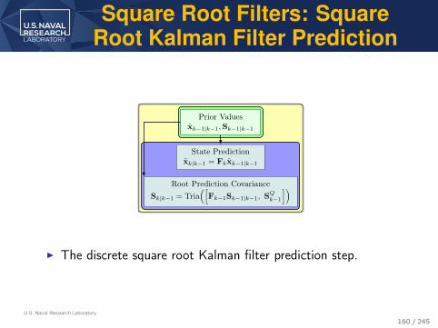
U.S. Naval Research Laboratory
Square Root Filters: SquareRoot Kalman Filter Prediction
Prior Valuesxk−1|k−1,Sk−1|k−1
State Predictionxk|k−1 = Fkxk−1|k−1
Root Prediction CovarianceSk|k−1 = Tria
([Fk−1Sk−1|k−1, SQ
k−1
])
I The discrete square root Kalman filter prediction step.
160 / 245

U.S. Naval Research Laboratory
Square Root Filters: SquareRoot CKF Update
Predicted Estimatesxk|k−1
Sk|k−1
Measurement Predictionzk|k−1 =
∑Nci=1 ωiz
(i)p
Innovationνk = zk − zk|k−1
Updated State Estimatexk|k = xk|k−1 + Wkνk
Predicted Cubature State Pointsx(i)p = xk|k−1 + Sk|k−1ξi
Predicted Cubature Measurement Pointsz(i)p = h
(x(i)p
)
Filter GainWk =
(Pxz
k|k−1/Szz′k|k−1
)/Szz
k|k−1
Updated Root State CovarianceSk|k = Tria
([(Xp −WkZp
), WkS
Rk
])
Base Cubature Points and WeightsChoose dx-dimensional cubature points {ξi} and weights
{ωi}
Centered, Predicted Cubature Point MatrixXp=
[√ω1(x
(1)p −xk|k−1), . . . ,
√ωNc (x
(Nc)p −xk|k−1)
]
Centered, Predicted Cubature Measurement Point MatrixZp=
[√ω1(z
(1)p −zk|k−1), . . . ,
√ωNc (z
(Nc)p −zk|k−1)
]
Root Innovation CovarianceSzz
k|k−1 = Tria([
Zp, SRk
])
Cross CovariancePxz
k|k−1 = XpZ′p
Measurementzk,S
Rk
I The square root CKF update is similar to the CKF updateutilizing Joseph’s form.
161 / 245

U.S. Naval Research Laboratory
Square Root Filters: SquareRoot EKF Update
Prior Predictionxk|k−1,Sk|k−1
Measurementzk,Rk
Jacobian
Hk =(∇xh
(xk|k−1
)′)′
Measurement Predictionzk|k−1 = h
(xk|k−1
)
Innovationνk = zk − zk|k−1
Root Innovation CovarianceSzzk|k−1 = Tria
([HkSk|k−1, SR
k
])
Cross CovariancePxz
k|k−1 = Sk|k−1S′k|k−1H′k
Filter GainWk =
(Pxz
k|k−1/Szz′k|k−1
)/Szz
k|k−1
Updated Square Root CovarianceSk|k = Tria
([(I−WkHk)Sk|k−1, WkS
Rk
])Updated State Estimatexk|k = xk|k−1 +Wkνk
I The square root EKF update.162 / 245

DIRECT FILTERING VERSUSMEASUREMENT CONVERSION
163 / 245

U.S. Naval Research Laboratory
Filtering Versus MeasurementConversion
I From what has been covered, two common approaches forbasic tracking exist:1. Cartesian converting measurements (and covariances) and
using a linear filter.2. Directly using measurements in a nonlinear filter.
I These shall be compared in a simple example.
164 / 245

U.S. Naval Research Laboratory
Filtering Versus MeasurementConversion
z
x−40−202040
200
20
−20
Ship 1
Ship 2Ship 3
Ship 4
Target
I A flat Earth.I All ships on the surface traveling−10m/s in the negative zdirection.
I The target initially at an altitudeof 7 km going 100m/s.
I Radars on ships pointed 15◦ upfrom the horizontal.
I q = 0.4802m2/s3
I Measurements every T = 0.5 s.I Tracks initialized via an
information filter with 2converted measurements.
I R12 = diag([10m, 10−2, 10−2]).
165 / 245

U.S. Naval Research Laboratory
Filtering Versus MeasurementConversion: RMSE
20 40 60 80 100 120 140 160 180 2000
500
1000
1500
2000
2500
3000
Time (seconds)
RM
SE
(m
ete
rs)
Monostatic
Monostatic PCRLB
Alternating 4 Tx
Alternating 4 Tx PCRLB
(a) Converted Measurements,RMSE
20 40 60 80 100 120 140 160 180 2000
500
1000
1500
2000
2500
3000
Time (seconds)
RM
SE
(m
ete
rs)
Monostatic
Monostatic PCRLB
Alternating 4 Tx
Alternating 4 Tx PCRLB
(b) EKF, RMSE
20 40 60 80 100 120 140 160 180 2000
500
1000
1500
2000
2500
3000
Time (seconds)
RM
SE
(m
ete
rs)
Monostatic
Monostatic PCRLB
Alternating 4 Tx
Alternating 4 Tx PCRLB
(c) CKF, RMSE
I The positional RMSE error of three different trackingalgorithms. The CKF used 5th order points.
I The CKF has the best RMSE performance.
166 / 245

U.S. Naval Research Laboratory
Filtering Versus MeasurementConversion: NEES
20 40 60 80 100 120 140 160 180 200
0.8
1
1.2
1.4
1.6
1.8
2
2.2
2.4
2.6
Time (seconds)
NE
ES
Monostatic
Alternating 4 Tx
(a) Converted Measurements,NEES
20 40 60 80 100 120 140 160 180 2000
200
400
600
800
1000
1200
Time (seconds)
NE
ES
Monostatic
Alternating 4 Tx
(b) EKF, NEES
20 40 60 80 100 120 140 160 180 200
0.8
1
1.2
1.4
1.6
1.8
2
2.2
2.4
2.6
Time (seconds)
NE
ES
Monostatic
Alternating 4 Tx
(c) CKF, NEES
I The NEES of three different tracking algorithms.I The EKF is bad; the CKF is the best over time; converted
measurements are initially the best.
167 / 245

DATA ASSOCIATION
168 / 245
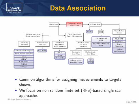
U.S. Naval Research Laboratory
Data Association
Data AssociationAlgorithms Multiple ScanSingle Scan
With IntegratedTrack Management
Without IntegratedTrack Management
ContinuityOver Time
No ContinuityOver Time
Random FiniteSet BasedMethods
TraditionalHypothesis-
Based Methods
PMHT MHTTrack Before
Detect
ContinuityOver Time
No ContinuityOver Time
Global Nearest Neighbor
Naïve Nearest Neighbor
JPDA
JPDA*GNN-JPDA
CJPDA
CJPDA*
Set JPDAJIPDA
JIPDA*GNN-JIPDA
Labeled Multi-Bernoulli Filter
PHDCPHD
Track-OrientedMHT
Hypothesis-OrientedMHT
ML-PDAFML-PMHT
HoughTransform
DynamicProgramming
I Common algorithms for assigning measurements to targetsshown.
I We focus on non random finite set (RFS)-based single scanapproaches.
169 / 245

U.S. Naval Research Laboratory
Data Association
Topics considered are:1. The Likelihood Function.2. Naïve Nearest Neighbor, the Score Function, and Global
Nearest Neighbor (GNN)3. Probabilistic Data Association (PDA) and Joint Probabilistic
Data Association (JPDA) variants
170 / 245
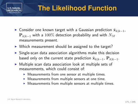
U.S. Naval Research Laboratory
The Likelihood Function
I Consider one known target with a Gaussian prediction xk|k−1,Pk|k−1 with a 100% detection probability and with NM
measurements present.I Which measurement should be assigned to the target?I Single-scan data association algorithms make this decision
based only on the current state prediction xk|k−1, Pk|k−1.I Multiple scan data association look at multiple sets of
measurements, which could consist of:I Measurements from one sensor at multiple times.I Measurements from multiple sensors at one time.I Measurements from multiple sensors at multiple times.
171 / 245
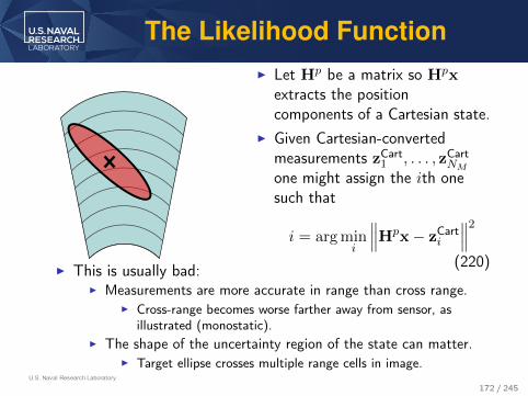
U.S. Naval Research Laboratory
The Likelihood FunctionI Let Hp be a matrix so Hpx
extracts the positioncomponents of a Cartesian state.
I Given Cartesian-convertedmeasurements zCart
1 , . . . , zCartNM
one might assign the ith onesuch that
i = arg mini
∥∥∥Hpx− zCarti
∥∥∥2
(220)I This is usually bad:
I Measurements are more accurate in range than cross range.I Cross-range becomes worse farther away from sensor, as
illustrated (monostatic).I The shape of the uncertainty region of the state can matter.
I Target ellipse crosses multiple range cells in image.
172 / 245
U.S. Naval Research Laboratory
The Likelihood Function
I One cannot convert the state to the measurement coordinatesystem and use a similar l2 norm.
I Mixing units (e.g. range, angle, and even range rate) makes nosense.
I Valid distance measures can be derived from likelihoodfunctions and likelihood ratios.
I Another reason that measurement covariance matrices matter.
I Let Zk−1 be the set of all measurements up to discrete timek − 1 and Θk−1 be the information of which measurementsare assigned to the track up to time k − 1.
I A valid cost function is the likelihood p(z|Zk−1,Θk−1).
173 / 245

U.S. Naval Research Laboratory
The Likelihood Function
I From the Law of Total Probability:
p(z|Zk−1,Θk−1) = p(z|x)p(x|Zk−1,Θk−1) (221)
I In all of the Kalman filter variants covered thus far
p(x|Zk−1,Θk−1) = N{x; xk|k−1,Pk|k−1
}(222)
I In the linear Kalman filter, the parameters for the productdistribution have already been computed. It can be shownthat:
p(z|x)p(x|Zk−1,Θk−1) = N{
z; z,Pzzk|k−1
}(223)
I In the CKF and EKF, the same expression is almost alwaysused to approximate the likelihood.
174 / 245

U.S. Naval Research Laboratory
The Likelihood Function
I Written out, the likelihood of the ith measurement:
p(zi|Zk−1,Θk−1) ,Λ(θi)
=∣∣∣2πPzz,i
k|k−1
∣∣∣− 12e− 1
2 (z−zk|k−1)′Pzz,ik|k−1(z−zk|k−1) (224)
I Pzz,ik|k−1 depends on the covariance matrix Ri of the ith
measurement.I Taking the negative logarithm of the likelihood and dropping
the normalizing constant terms and 1/2 scale factor one has aMahalanobis distance:
− log(
Λ(θi))∝(z− zk|k−1
)′Pzz,ik|k−1
(z− zk|k−1
)(225)
I From the mathematics section, we know that Mahalanobisdistances can be used for chi-squared testing to determinewhether measurements can even be considered valid.
I The exclusion of measurements from possible assignments isgating.
175 / 245

U.S. Naval Research Laboratory
The Likelihood Function
I If one target is present and R is the same for allmeasurements, the maximum likelihood (ML) assignment hasthe minimum Mahalanobis distance.
I If R varies between measurements, this is not the case!I For a counter example:
I Consider two scalar Gaussian distributions: N{z1; 0, σ2
1
}and
N{z2; 0, σ2
2
}.
I Choose z1 = 1, σ1 = 1, σ22 = e−10, z22 = 8e−10.
I One observes that
z21σ21
<z22σ22
⇐⇒ 1 < 8 (226)
(2πσ2
1
)− 12 e− z21
2σ21 <(2πσ2
2
)− 12 e− z22
2σ22 ⇐⇒ 1√2πe
<e√2π
(227)
I For a predicted measurement of zero, the Mahalanobisdistance choice disagrees with the ML choice.
176 / 245

U.S. Naval Research Laboratory
The Likelihood Function
I To choose the ML measurement for assignment:I Use the likelihood function if measurement covariance matrices
vary.I Use the Mahalanobis distance when all measurements have the
same covariance matrix.
I The Mahalanobis distance can be used for gating regardless ofwhether the accuracies vary.
I What if multiple targets are present?
177 / 245
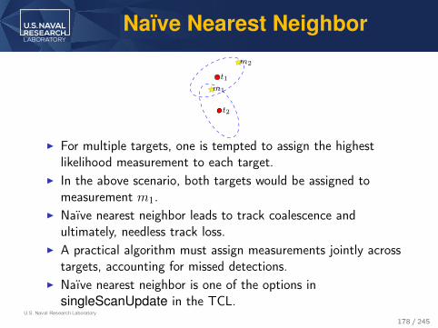
U.S. Naval Research Laboratory
Naïve Nearest Neighbor
t1
t2
m1
m2
I For multiple targets, one is tempted to assign the highestlikelihood measurement to each target.
I In the above scenario, both targets would be assigned tomeasurement m1.
I Naïve nearest neighbor leads to track coalescence andultimately, needless track loss.
I A practical algorithm must assign measurements jointly acrosstargets, accounting for missed detections.
I Naïve nearest neighbor is one of the options insingleScanUpdate in the TCL.
178 / 245

U.S. Naval Research Laboratory
The Score Function
I We want to derive a cost function (a score function) that canbe used for multiple target assignment.
I The exponential of the score function derived here is computedin makeStandardLRMatHyps andmakeStandardCartOnlyLRMatHyps in the TCL.
I DefineI θ as an assignment of measurements to targets at a given time.I Z = {z1, . . . , zm} is the current set of observations.I m is the cardinality of Z.I Ip is all prior information.
I One can write:Pr {θ, Ip|Z} = Pr {θ, Ip|Z,m} m adds no new information (228)
=1
c1p(Z|m, θ, Ip) Pr {θ, Ip|m} Bayes’ Theorem (229)
=1
c1p(Z|m, θ, Ip) Pr {θ|m, Ip}Pr {Ip|m} Conditional Probability (230)
179 / 245
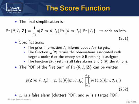
U.S. Naval Research Laboratory
The Score Function
I The final simplification is
Pr {θ, Ip|Z} =1
c1p(Z|m, θ, Ip) Pr {θ|m, Ip}Pr {Ip} m adds no info
(231)I Specifications:
I The prior information Ip informs about NT targets.I The function ξt(θ) return the observations associated with
target t under θ or the empty set ∅ if nothing is assigned.I The function ξ(θ) returns all false alarms and ξi(θ) the ith one.
I The PDF of the first term of Pr {θ, Ip|Z} can be written
p(Z|m, θ, Ip) = pc(ξ(θ)|m, θ, Ip
) NT∏
i=1
pt (ξt(θ)|m, θ, Ip)
(232)I pc is a false alarm (clutter) PDF, and pt is a target PDF.
180 / 245

U.S. Naval Research Laboratory
The Score Function
I The target PDF is
pt (ξt(θ)|m, θ, Ip) =
{1 if ξt(θ) = �
pt (ξt(θ)|m, θ, Ip) otherwise(233)
where pt (ξt(θ)|m, θ, Ip) equals the previously developedlikelihood of a measurement assigned to a target given thepredicted state.
I If all false alarms are independent,
pc(ξ(θ)|m, θ, Ip
)=
φ(θ)∏
i=1
pc(ξi(θ)|m, θ, Ip
). (234)
where φ(θ) is the number of false alarms in hypothesis θ.
181 / 245

U.S. Naval Research Laboratory
The Score Function
I Define δ(θ) as a set of Boolean detection indicators for theassociation hypothesis θ such that δt(θ) = 1 if target t wasobserved.
I The PDF of the second term of Pr {θ, Ip|Z} can be written
Pr {θ|m, Ip} = Pr {θ|m, Ip, δ(θ), φ(θ)}Pr {δ(θ), φ(θ)|m, Ip}(235)
using the Law of Total Probability.I The first term of (235) is the probability of an association of
measurements to targets given one knows which targets havebeen observed and how many measurements are present.
182 / 245

U.S. Naval Research Laboratory
The Score Function
I Without the actual measurements given and with Ippresumably uninformative, all possibilities are equiprobable:
Pr {θ|m, Ip, δ(θ), φ(θ)} =
Choose measurementsoriginating from targets︷ ︸︸ ︷(
m
m− φ (θ)
)Assign chosen measurements
to targets︷ ︸︸ ︷(m− φ (θ))!
−1
(236)
=φ(θ)!
m!(237)
where it was assumed that m− φ(θ) ≥ 0, i.e. that thehypothesis in question is valid.
183 / 245

U.S. Naval Research Laboratory
The Score FunctionI Suppressing the argument (θ) in δ and φ, and letting P tD be
the detection probability of target t, the second term ofPr {θ|m, Ip} is
Pr {δ, φ|m, Ip} = Pr {δ|m,φ, Ip}Pr {φ|m, Ip} (238)
=
(Pr {δ
⋂(m− φ) targets seen|φ, Ip}
Pr {(m(k)− φ) targets seen|φ, Ip}
)·(
Pr {m|φ, Ip}Pr{φ}Pr{m}
)(239)
=
( ∏NTt=1
(P tD)δt (1− P tD)1−δt
Pr {(m(k)− φ) targets seen|φ, Ip}
)
·(
Pr {(m(k)− φ) targets seen|φ, Ip}Pr{φ}Pr{m}
)(240)
=Pr{φ}Pr{m}
NT∏t=1
(P tD)δt
(1− P tD)1−δt (241)
I In(240), the prior information Ip informs on P tD.184 / 245

U.S. Naval Research Laboratory
The Score Function: P tD
I P tD can be set as a nominal design parameter.I Never set P t
D to 1.
I Often, P tD is approximated based on observed targetamplitudes over time.
I P tD can also be estimated by fitting to a stochastic radar crosssection model and using the radar range equation.
I The Swerling models in “MathematicalFunctions/Statistics/Detection Statistics/” in the TCL canhelp determine P tD from stochastic target power models.
185 / 245

U.S. Naval Research Laboratory
The Score Function
I Combining expressions for the terms of Pr {θ|m, Ip}, one gets
Pr {θ|m, Ip} =φ!
m!
Pr{φ}Pr{m}
NT∏
t=1
(P tD)δt (1− P tD)1−δt (242)
I Substituting that and the other terms back into the expressionfor Pr{θ, Ip|Z} leads to
Pr{θ, Ip|Z} =φ! Pr{φ}
c2
φ∏
i=1
pc(ξi|m, θ, Ip
)
·NT∏
t=1
(P tDpt (ξt|m, θ, Ip)
)δt (1− P tD)1−δt Pr {Ip} (243)
where missing normalization terms are in c2.186 / 245

U.S. Naval Research Laboratory
The Score Function
I Dividing out the clutter PDF for measurements assigned totargets:
Pr{θ, Ip|Z} =φ! Pr{φ}
c3Pr {Ip}
·NT∏
t=1
(P tD
pt (ξt|m, θ, Ip)pc (ξt|m, θ, Ip)
)δt(1− P tD)1−δt
(244)
I We want to get rid of the φ! Pr{φ} term.I Assume a constant false alarm density λ over the observation
volume V , with false alarms from a Poisson process. Then
Pr{φ} = e−λλφ
φ!. (245)
with λ = λV .187 / 245

U.S. Naval Research Laboratory
The Score Function
I Substituting the false alarm model:
Pr{θ, Ip|Z} =1
c4Pr {Ip}
NT∏t=1
(P tD
pt (ξt|m, θ, Ip)(λV )pc (ξt|m, θ, Ip)
)δt(1− P tD)1−δt
(246)
I It is generally undesirable to have to compute the volume V .The volume can be eliminated assuming that false alarms areuniformly distributed in the observation region:
pc (ξt|m, θ, Ip) =1
V(247)
188 / 245

U.S. Naval Research Laboratory
The Score Function
I The result of a uniform false alarm model is:
Pr{θ, Ip|Z} =1
c4Pr {Ip}
NT∏t=1
(P tD
pt (ξt|m, θ, Ip)λ
)δt(1− P tD)1−δt
(248)
I Taking the logarithm of Pr{θ, Ip|Z} and discarding constantterms, one gets
ln {Pr{θ, Ip|Z}} ∝ Λ(θ) =
NT∑t=1
δt ln
(P tD
pt (ξt|m, θ, Ip)λ
)+ (1− δt) ln(1− P tD)
(249)
189 / 245
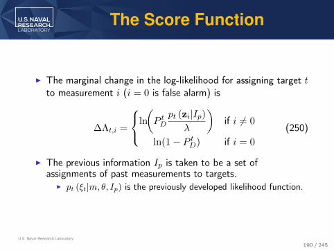
U.S. Naval Research Laboratory
The Score Function
I The marginal change in the log-likelihood for assigning target tto measurement i (i = 0 is false alarm) is
∆Λt,i =
ln
(P tD
pt (zi|Ip)λ
)if i 6= 0
ln(1− P tD) if i = 0
(250)
I The previous information Ip is taken to be a set ofassignments of past measurements to targets.
I pt (ξt|m, θ, Ip) is the previously developed likelihood function.
190 / 245

U.S. Naval Research Laboratory
The Score Function
I Assuming a Gaussian prior, the marginal change in thelog-likelihood is
∆Λt,i =
ln
P tD
N{
zi, ztk|k−1,P
zz,i,tk|k−1
}
λ
if i 6= 0
ln(1− P tD) if i = 0
(251)
I ztk|k−1 is the predicted measurement from the tth target,I Pzz,i,t
k|k−1 is the innovation covariance the for ith measurementand tth target.
I The term ∆Λt,i is the marginal score function for single-frameassignment.
I Summing the marginals for a full target-measurementassignment, one forms the full score function Λ(θ) for a scan.
191 / 245

U.S. Naval Research Laboratory
The Score Function
I When using a converted measurement filter, the units ofN{
zi, ztk|k−1,P
zz,i,tk|k−1
}are in Cartesian coordinates, but the
units of λ are usually in the radar’s local coordinates.I The proper conversion of λ to Cartesian coordinates yields a
different λ at every point.I Cartesian λ is higher closer to the sensor.
I We want to derive what the Cartesian version of λ given λ inthe measurement coordinate system.
192 / 245

U.S. Naval Research Laboratory
The Score Function:Converting λ
I Say x = fx(y).I Volume integrals in each system are related by
∫
x∈Sx
dx =
∫
y∈Sy
|J(y)|dy (252)
where Sx and Sy are the same regions, but in differentcoordinate systems and J is the Jacobian:
J(y) =
[∂
∂y1fx(y),
∂
∂y2fx(y), . . . ,
∂
∂ydyfx(y)
](253)
193 / 245
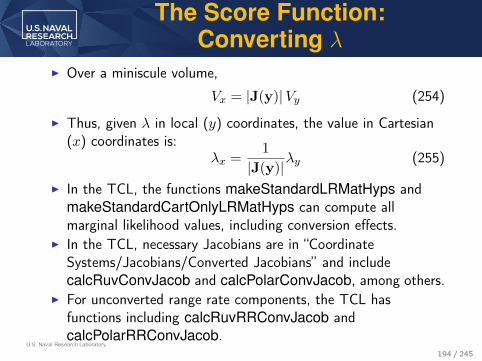
U.S. Naval Research Laboratory
The Score Function:Converting λ
I Over a miniscule volume,
Vx = |J(y)|Vy (254)
I Thus, given λ in local (y) coordinates, the value in Cartesian(x) coordinates is:
λx =1
|J(y)|λy (255)
I In the TCL, the functions makeStandardLRMatHyps andmakeStandardCartOnlyLRMatHyps can compute allmarginal likelihood values, including conversion effects.
I In the TCL, necessary Jacobians are in “CoordinateSystems/Jacobians/Converted Jacobians” and includecalcRuvConvJacob and calcPolarConvJacob, among others.
I For unconverted range rate components, the TCL hasfunctions including calcRuvRRConvJacob andcalcPolarRRConvJacob.
194 / 245

U.S. Naval Research Laboratory
GNN Assignment
I One could assign measurements to targets and false alarms bychoosing the assignment θ that maximizes the score function.
I How many valid assignments are there for m measurement andNT targets?
Nhyp =
min(m,NT )∑
l=0︸ ︷︷ ︸Sum over the numberof targets observed
Choose which targetsare observed︷ ︸︸ ︷(
NT
l
) (m
l
)
︸ ︷︷ ︸Choose which measurements
are not false alarms
Assign the measurementsto the targets︷︸︸︷
l! (256)
I Suppose there are 3000 measurements and targets, and nofalse alarms or missed detections.
I There are 3000! ≈ 4.14× 109130 hypotheses.I This is about one googol (10100) raised to 91.3.
195 / 245

U.S. Naval Research Laboratory
GNN Assignment
I The most power supercomputer (Tianhe-2, China) is 33.85petaflops.
I A lower bound of execution time is one floating pointoperation per hypothesis.
I It would take over 3.88× 109106 years to visit each hypothesis.I However, one can optimally solve the assignment problem in
under 4 seconds (worst case) on an old laptop.I In much of tracking, one cannot formulate an optimal solution
and tell a first semester programmer to make it fast using aGPU or FPGA.
I Techniques from theoretic computer science are required forcomputational feasibility.
196 / 245

U.S. Naval Research Laboratory
GNN Assignment
I There are 3000! ≈ 4.14× 109130 hypotheses, but only30002 = 9× 10⁶ marginal hypotheses (values of ∆Λt,i).
I The efficient solution is formulated as a GNN assignment (2Dassignment) problem:
x∗ = arg maxx
NR∑i=1
NC∑j=1
∆Λi,jxi,j (257)
subject toNC∑j=1
xi,j = 1 ∀i Every target is assignedto an event.
(258)
NR∑i=1
xi,j ≤ 1 ∀j Not every event isassigned to a target.
(259)
xi,j ∈ {0, 1} ∀xi,jEquivalent toxi,j ≥ 0 ∀xi,j
(260)
I NR = NT and NC = NT +m, number of measurements plusmissed detection hypotheses.
197 / 245
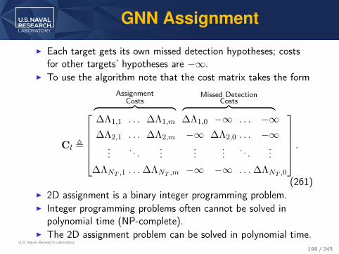
U.S. Naval Research Laboratory
GNN Assignment
I Each target gets its own missed detection hypotheses; costsfor other targets’ hypotheses are −∞.
I To use the algorithm note that the cost matrix takes the formAssignment
Costs︷ ︸︸ ︷Missed Detection
Costs︷ ︸︸ ︷
Cl ,
∆Λ1,1 . . . ∆Λ1,m ∆Λ1,0 −∞ . . . −∞∆Λ2,1 . . . ∆Λ2,m −∞ ∆Λ2,0 . . . −∞
.... . .
......
.... . .
...∆ΛNT ,1 . . .∆ΛNT ,m −∞ −∞ . . .∆ΛNT ,0
.
(261)I 2D assignment is a binary integer programming problem.I Integer programming problems often cannot be solved in
polynomial time (NP-complete).I The 2D assignment problem can be solved in polynomial time.
198 / 245
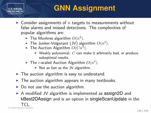
U.S. Naval Research Laboratory
GNN Assignment
I Consider assignments of n targets to measurements withoutfalse alarms and missed detections. The complexities ofpopular algorithms are:
I The Munkres algorithm O(n4).I The Jonker-Volgenant (JV) algorithm O(n3).I The Auction Algorithm O(Cn3).
I Weakly polynomial. C can make it arbitrarily bad, or producesuboptimal results.
I The ε-scaled Auction Algorithm O(n3).I Not as fast as the JV algorithm.
I The auction algorithm is easy to understand.I The auction algorithm appears in many textbooks.I Do not use the auction algorithm.I A modified JV algorithm is implemented as assign2D and
kBest2DAssign and is an option in singleScanUpdate in theTCL.
199 / 245

U.S. Naval Research Laboratory
GNN Assignment
I The Jonker-Volgenant-Castañon (JVC) algorithm is popular inthe tracking literature.
I Castañon published a rectangular (possible missed detections)JV modification.
I The JVC algorithm is popular because code is provided.I The algorithm initializes a rectangular JV algorithm with an
auction algorithm.I The ε term in the auction algorithm can cause the JV
algorithm to sometimes produce suboptimal results.I The auction algorithm initialization is not necessary; don’t use
the JVC algorithm.
I A rectangular modification to the JV algorithm, is derived inD. F. Crouse, “On Implementing 2D Rectangular Assignment Algorithms,” IEEE Transactions onAerospace and Electronic Systems, vol. 52, no. 4, pp. 1679-1696, Aug. 2016.
I The derivation is lengthy, involves Lagrangian relaxation anddual-primal optimization and is omitted here.
200 / 245

U.S. Naval Research Laboratory
The PDA and JPDA Algorithms
I The GNN algorithm is a maximum-likelihood approach.I An alternative is to use the expected value over all possible
target-measurement assignments.I For a single target, the expected value and the covariance of
the estimate are called probabilistic data association (PDA).I For multiple targets, it is called Joint Probabilistic Data
Association (JPDA).I Variants of the PDA and JPDA are implemented in
singleScanUpdate in the TCL.
201 / 245

U.S. Naval Research Laboratory
The PDA and JPDA Algorithms
I For the tth target, the JPDA update is
xtk|k = E{xtk |Z, Ip
}=
m∑
i=0
βi,txt,ik|k (262)
Ptk|k = E
{(xtk − xtk|k
)(xtk − xtk|k
)′∣∣∣∣Z, Ip}
(263)
=
m∑
i=0
βi,t(
Pt,ik|k +
(xt,ik − xtk|k
)(xt,ik − xtk|k
)′)(264)
I βi,t is the probability of assigning measurement i to target t (0is a missed detection).
I Superscripts of i and t indicate measurement and targethypotheses.
I Ip is information on the (assumed Gaussian) prior estimates.I The literature often uses a simpler expression for Pt
k|k that isnot quadratic in form and subject to finite precision errors.
202 / 245

U.S. Naval Research Laboratory
The PDA and JPDA Algorithms
I Assumptions going into the PDA/JPDA are that the priordistributions on all targets are Gaussian.
I The covariance cross terms between targets are not zero, butare omitted.
I JPDA variants including cross terms begin with a C forcoupled.
I Including the cross terms worsens the performance (worsenstrack coalescence).
I The hardest part of the PDA/JPDA is the computation of theβ values.
203 / 245

U.S. Naval Research Laboratory
The PDA and JPDA Algorithms
I TIt was shown that the probability going into the scorefunction can be expanded:
Pr {θ, Ip|Z} =1
c1p(Z|m, θ, Ip) Pr {θ|m, Ip}Pr {Ip} (265)
I In the JPDA, we assume that the prior information is fixed(Gaussian distributions, not multiple hypotheses). Thus,Pr {Ip} = 1, so
Pr {θ, Ip|Z} =1
c1p(Z|m, θ, Ip) Pr {θ|m, Ip} (266)
= Pr {θ|Z, Ip} (267)
I This means that the previously derived Pr {θ, Ip|Z} can beused to compute the β terms.
204 / 245
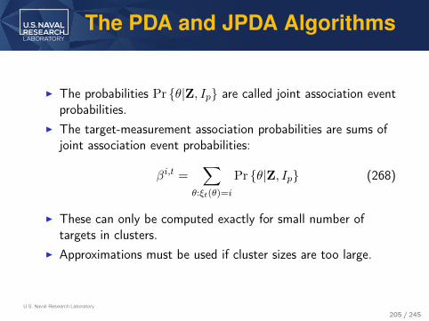
U.S. Naval Research Laboratory
The PDA and JPDA Algorithms
I The probabilities Pr {θ|Z, Ip} are called joint association eventprobabilities.
I The target-measurement association probabilities are sums ofjoint association event probabilities:
βi,t =∑
θ:ξt(θ)=i
Pr {θ|Z, Ip} (268)
I These can only be computed exactly for small number oftargets in clusters.
I Approximations must be used if cluster sizes are too large.
205 / 245

U.S. Naval Research Laboratory
The PDA and JPDA Algorithms
t1
t2
t3
t4m1m2
m3
m4
m6m5
m7
m8
I Gating and clustering are important parts of a large-scaleJPDA implementation.
I In the above figure, measurements are said to gate with atarget if in the ellipse overlaps them.
I In practice, use a chi-squared test on the Mahalanobis distance.I There are three clusters of targets and measurements.
1. Target t1 is in a cluster with m4.2. Targets t2 and t3 (linked by m2) cluster with m1, m2, and m3.3. Target t4 is in a cluster with m6.
206 / 245

U.S. Naval Research Laboratory
The PDA and JPDA Algorithms
I Targets are in a common cluster if they contest ameasurement.
I Measurements are associated with clusters.I Separate clusters of targets/ measurements can be processed
by separate JPDAs.I The β values for small clusters can be determined exactly.I The β values of large clusters must be approximated.
207 / 245
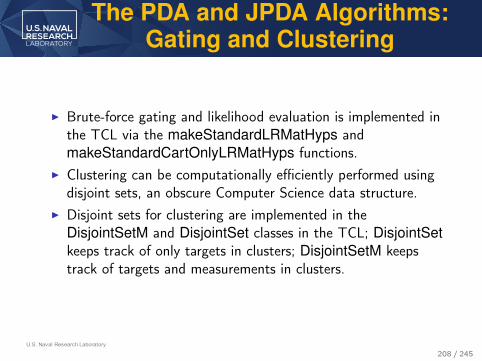
U.S. Naval Research Laboratory
The PDA and JPDA Algorithms:Gating and Clustering
I Brute-force gating and likelihood evaluation is implemented inthe TCL via the makeStandardLRMatHyps andmakeStandardCartOnlyLRMatHyps functions.
I Clustering can be computationally efficiently performed usingdisjoint sets, an obscure Computer Science data structure.
I Disjoint sets for clustering are implemented in theDisjointSetM and DisjointSet classes in the TCL; DisjointSetkeeps track of only targets in clusters; DisjointSetM keepstrack of targets and measurements in clusters.
208 / 245

U.S. Naval Research Laboratory
The PDA and JPDA Algorithms:Gating and Clustering
Outputs
Inputs
Outputs
Inputs
P1 P2 . . . Pg
Perform Gating and Clustering
Initial Estimatesxtk|k−1
,Ptk|k−1
Observationszi
Combine Cluster Estimatesxtk|k,P
tk|k
Processing Group Pg
Calculateβi,t ∀(i, t) ∈ Gg
Calculate
xi,tk|k,P
i,tk|k ∀(i, t) ∈ Gg
Clustered Targetsxtk|k−1
Ptk|k−1
∀(t) ∈ Gg
Gated Observationszi ∀(i) ∈ Gg
Calculatextk|k,P
tk|k ∀(i, t) ∈ Gg
I An illustration go how separate clusters can be processedindependently.
I Gg is the set of targets and measurements in the gth cluster.
209 / 245

U.S. Naval Research Laboratory
The PDA and JPDA Algorithms:Computing β
I When the β terms must be computed exactly, two approachesshall be considered:1. Via brute-force evaluation of all joint association events.2. Via matrix permanents.
I The matrix permanent approach is faster, but brute force isnecessary to derive some JPDAF variants.
210 / 245

U.S. Naval Research Laboratory
The PDA and JPDA Algorithms:Computing β
I Brute-force evaluation adds all joint association events θ andadds the (usually unnormalized) probabilities Pr {θ|Z, Ip} tothe appropriate βi,t terms.
I Normalization can be done afterwards. If βi,t are theunnormalized association probabilities, then
βi,t =βi,t∑mj=1 βj,t
(269)
I The brute force method can be implemented as four nestedloops:1. Choose how many targets are observed.2. Choose which targets are observed.3. Choose which measurements originated from targets.4. Permute all associations of observed targets to
target-originated measurements.
211 / 245

U.S. Naval Research Laboratory
The PDA and JPDA Algorithms:Computing β
I To compute the necessary combinations and permutations forthe brute-force method, many of the functions in the folder“Mathematical Functions/Combinatorics” of the TCL can beused. These include genNextCombo andunrankCombination, and unrankPermutation, among manyothers.
I The determinant of a square matrix is often taught as
|A| =∑
σ∈Snsgn(σ)
n∏
i=1
ai,σi (270)
where Sn is the set of all permutations of the values 1 to nand sign(σ) is the sign (a.k.a. signature or parity) of thepermutation.
212 / 245
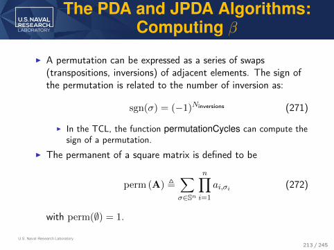
U.S. Naval Research Laboratory
The PDA and JPDA Algorithms:Computing β
I A permutation can be expressed as a series of swaps(transpositions, inversions) of adjacent elements. The sign ofthe permutation is related to the number of inversion as:
sgn(σ) = (−1)Ninversions (271)
I In the TCL, the function permutationCycles can compute thesign of a permutation.
I The permanent of a square matrix is defined to be
perm (A) ,∑
σ∈Sn
n∏
i=1
ai,σi (272)
with perm(∅) = 1.
213 / 245

U.S. Naval Research Laboratory
The PDA and JPDA Algorithms:Computing β
I The permanent of a square matrix is the determinant withoutthe − signs.
I The permanent of a square matrix is the sum of the productsof all combinations selecting one element from each row andcolumn.
I The permanent of a rectangular m× n matrix with m ≤ n isalso defined as
perm (A) ,∑
σ∈Pn,m
m∏
i=1
ai,σi (273)
where Pn,m is the set of all length m permutations of n items(known as arrangements).
I The permanent of a rectangular m× n matrix with m ≤ n isthe sum of the product of all arrangements selecting one itemfrom each row and at most one item from each column.
214 / 245

U.S. Naval Research Laboratory
The PDA and JPDA Algorithms:Computing β
I Consider a matrix of likelihoods with ∆Λt,i = e∆Λt,i ,non-normalized assignment probabilities:
C:AssignmentLikelihoods︷ ︸︸ ︷
Missed DetectionLikelihoods︷ ︸︸ ︷
C ,
∆Λ1,1 . . . ∆Λ1,m ∆Λ1,0 0 . . . 0
∆Λ2,1 . . . ∆Λ2,m 0 ∆Λ2,0 . . . 0...
. . ....
......
. . ....
∆ΛNT ,1 . . . ∆ΛNT ,m 0 0 . . . ∆ΛNT ,0
(274)I The normalized expression for the β terms can be rewritten
directly in terms of likelihoods using elements of C:
βj,k = ∆Λj,k
∑σ∈PNT−1,NT−1+m
∏NTn=1n 6=j
cn,σn
∑σ∈PNT ,NT+m
∏NTn=1 cn,σn
(275)
215 / 245

U.S. Naval Research Laboratory
The PDA and JPDA Algorithms:Computing β
I The expression simplifies to
βj,k = ∆Λj,kperm
(Cj,k
)
perm (C)(276)
where Cj,k is the matrix C after removing row j and columnk.
I The matrix determinant can be evaluated in polynomial timeusing Gaussian elimination.
I The matrix permanent cannot be evaluated in polynomial timeunless P=NP.
I The relation between P and NP complexity classes is a majorunsolved problem in theoretical computer science.
I Efficient exponential complexity algorithms exist. In the TCL,the function perm implements an efficient algorithm.
216 / 245

U.S. Naval Research Laboratory
The PDA and JPDA Algorithms
I Functions to explicitly compute the β values are implementedin the calc2DAssignmentProbs function in the TCL.
I Many techniques to approximate β values exist and areimplemented in calc2DAssignmentProbsApprox in the TCL.
I Methods to do the complete PDA and JPDA update are givenin singleScanUpdate in the TCL.
I However, one usually uses a variant of the JPDA algorithmrather than the JPDA algorithm itself.
217 / 245
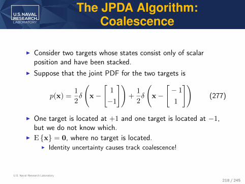
U.S. Naval Research Laboratory
The JPDA Algorithm:Coalescence
I Consider two targets whose states consist only of scalarposition and have been stacked.
I Suppose that the joint PDF for the two targets is
p(x) =1
2δ
(x−
[1
−1
])+
1
2δ
(x−
[− 1
1
])(277)
I One target is located at +1 and one target is located at −1,but we do not know which.
I E {x} = 0, where no target is located.I Identity uncertainty causes track coalescence!
218 / 245

U.S. Naval Research Laboratory
The JPDA Algorithm:Coalescence
1000 500 0 500 1000 1500 2000 2500 3000600
400
200
0
200
400
600
x [m]
y [m
]
The JPDAF
I Target identity is important, but we really want to know wherethings are.
I The above plot is typical of targets remaining close for manyscans in the JPDA filter.
219 / 245

U.S. Naval Research Laboratory
The JPDA Algorithm:Coalescence
(a) Prior toPrediction
(b) AfterPrediction
I Targets can be “too close” in the JPDAF even when wellresolved by the sensor.
I Closeness is related to predicted target uncertainty.I Well-separated targets becomes “too close” if prediction
interval is too large.220 / 245

U.S. Naval Research Laboratory
The JPDA Algorithm:Coalescence
I Coalescence is not a “bias”.I Coalescence is the result of using the expected value given
uncertain identity.I The expected value is a minimum mean squared error (MMSE)
estimate.I A form of the minimum mean optimal subpattern assignment
(MMOSPA) method:I Avoids the coalescence of the expected value.I Still has the same smoothing properties as the expected value
versus ML.
221 / 245
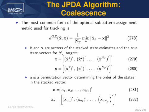
U.S. Naval Research Laboratory
The JPDA Algorithm:Coalescence
I The most common form of the optimal subpattern assignmentmetric used for tracking is
dOE(x,x) =1
NTmina‖xa − x‖2 (278)
I x and x are vectors of the stacked state estimates and the truestate vectors for NT targets:
x =[(
x1)′,(x2)′, . . . ,
(xNT
)′]′(279)
x =[(
x1)′,(x2)′, . . . ,
(xNT
)′]′(280)
I a is a permutation vector determining the order of the statesin the stacked vector:
a = [a1, a2, . . . , aNT ]′ (281)
xa =
[(xa1)
′, (xa2)
′, . . . ,
(xaNT
)′]′(282)
222 / 245
U.S. Naval Research Laboratory
The JPDA Algorithm:Coalescence
I MMOSPA estimation is essentially an expected value withtarget identity removed.
I Typically, the ordering for the MMOSPA estimate is computedonly using position components of the state.
I The strict OSPA definition mixes unlike units (e.g. positionand velocity).
I The Set JPDAF is an approximate MMOSPA estimator.I In the TCL, use calcSetJPDAUpdate to use the Set JPDAF.
It is also an option in singleScanUpdate.I An approximate MMOSPA estimator is given in
MMOSPAApprox in the TCL.
223 / 245

U.S. Naval Research Laboratory
The JPDA Algorithm:Coalescence
I In practice, the Set JPDAF is not usedI It discards too much identity information.I It is slower than alternatives.
I Two common alternatives to resist coalescence are1. The GNN-JPDA2. The JPDA*
224 / 245

U.S. Naval Research Laboratory
The JPDA Algorithm:Coalescence
I The GNN-JPDA is simple:1. Determine the measurement to use with a GNN filter, giving
xk|k.2. Compute Pk|k as in the JPDA, using the GNN estimate as the
mean xk|k.
I The hard assignment avoids coalescence.I Computing Pk|k as a MSE matrix improves covariance
consistency/reduces track loss.I Available as an option in singleScanUpdate in the TCL with
exact and approximate βs.
225 / 245
U.S. Naval Research Laboratory
The JPDA Algorithm:Coalescence
I The brute-force computation of the βs had loops:1. Choose how many targets are observed.2. Choose which targets are observed.3. Choose which measurements originated from targets.4. Permute all associations of observed targets to
target-originated measurements.I The JPDA* is the same as the JPDA except in the innermost
loop, only the maximum likelihood permutation is used.I Has the smoothing of the expected value.I The hard decision gets rid of identity uncertainty: Resistant to
coalescence.
I Use calcStarBetasBF for the βs in the TCL. Available as anoption in singleScanUpdate in the TCL.
226 / 245

U.S. Naval Research Laboratory
The JPDA Algorithm: Example
-6 -4 -2 0 2 4
x meters 104
-4
-3
-2
-1
0
1
2
3
4
y m
ete
rs
104 True and Estimated Trajectories
I A 2D example of the JPDA* including gating and clustering isgiven in demo2DDataAssociation in “Sample Code/BasicTracking Example" in the TCL.
I A sample run is shown above. Tracks were started from twocued measurements.
I Estimated tracks: Red. True track: Dashed black. Detections:Blue. Very resistant to false alarms.
227 / 245

CASCADED LOGIC AND INTEGRATEDTRACKERS
228 / 245

U.S. Naval Research Laboratory
Cascaded Logic and IntegratedTrackers
I The GNN and JPDA algorithms only update established tracks.I Most practical systems require the ability to start and
terminate tracks.I Two main categories of algorithms exist for single-scan data
association approaches:I Cascaded Logic Trackers
I Confirmed-tracks, pre-tracks and hard decisions for initiationand termination.
I Integrated TrackersI Lots of targets, each with a probability of existing.
229 / 245

U.S. Naval Research Laboratory
A Cascaded Logic Tracker
Predicted States, Scoresxtk|k−1,P
tk|k−1,Λ
tk−1
Confirmed Tracks
Measurementszi,Ri
Single Scan Updatee.g. JPDA
on Confirmed Tracks
Determine GNNAssignment
on Confirmed Tracks
Terminate ConfirmedTracks FailingPage’s Test
UpdateCumulative Scores Λt
on Confirmed Tracks
Single Scan Updatee.g. JPDA
on Candidate Tracks
Predicted States, Scoresxt,pk|k−1,P
t,pk|k−1,Λ
t,p
Candidate Tracks
Determine GNNAssignment
on Candidate Tracks
Promote or TerminateCandidate Tracks Based
on the SPRT
UpdateCumulative Scores Λt
p
on Candidate Tracks
One-Point Initializationand Initial Score
for New Candidate Tracks
Unassigned Measurements
Unassigned Measurements
Unassigned Measurements
I Multiple Types ofcascaded logic trackersexist.
I There are confirmedtracks and candidatetracks.
I Sometimespre-tracks too.
I Scores usually updatedvia GNN assignments.
I Measurements not inGNN assignments goon to the next stage.
I Creation, promotionand deletion of tracksin purple-outlinedboxes.
230 / 245

U.S. Naval Research Laboratory
A Cascaded Logic Tracker
I Measurements not assigned to confirmed tracks or candidatetracks become new candidate tracks via single pointinitialization.
I New candidate tracks assigned an initial track score Λtp.I As candidate tracks are updated with measurements, the
likelihood increment ∆Λt of the GNN hypothesis for that trackis added to Λtp.
I A sequential probability ratio test (SPRT) determines whetherto declare the track confirmed or false.
231 / 245

U.S. Naval Research Laboratory
A Cascaded Logic Tracker: TheSPRT
I Let pm(Zm|θ) be the conditional PDF of a track given mmeasurements in Zm under the hypothesis θ that the trackexists.
I pm(Zm|∅) be the conditional PDF of false alarms given mmeasurements in Zm under the hypothesis that no track exists.
I A conditional probability ratio is
lm(Zm) =pm(Zm|θ)pm(Zm|∅)
(283)
I We choose two positive constants a and b such that at stepm:
I If a > lm(Zm) > b the test continue for another step.I If a ≤ lm(Zm), it is declared there is a track.I If b ≥ lm(Zm), it is declared there is no track.
I This test is the SPRT for likelihood ratios.232 / 245
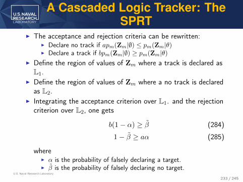
U.S. Naval Research Laboratory
A Cascaded Logic Tracker: TheSPRT
I The acceptance and rejection criteria can be rewritten:I Declare no track if apm(Zm|∅) ≤ pm(Zm|θ)I Declare a track if bpm(Zm|∅) ≥ pm(Zm|θ)
I Define the region of values of Zm where a track is declared asL1.
I Define the region of values of Zm where a no track is declaredas L2.
I Integrating the acceptance criterion over L1. and the rejectioncriterion over L2, one gets
b(1− α) ≥ β (284)
1− β ≥ aα (285)
whereI α is the probability of falsely declaring a target.I β is the probability of falsely declaring no target.
233 / 245
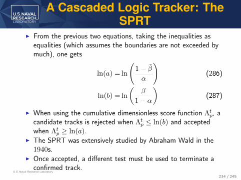
U.S. Naval Research Laboratory
A Cascaded Logic Tracker: TheSPRT
I From the previous two equations, taking the inequalities asequalities (which assumes the boundaries are not exceeded bymuch), one gets
ln(a) = ln
(1− βα
)(286)
ln(b) = ln
(β
1− α
)(287)
I When using the cumulative dimensionless score function Λtp, acandidate tracks is rejected when Λtp ≤ ln(b) and acceptedwhen Λtp ≥ ln(a).
I The SPRT was extensively studied by Abraham Wald in the1940s.
I Once accepted, a different test must be used to terminate aconfirmed track.
234 / 245

U.S. Naval Research Laboratory
A Cascaded Logic Tracker: TheSPRT
I If the SPRT were continued after confirmation, the cumulativescore would generally keep increasing.
I When a track ends, the score would need to come back downto terminate if one tried to continue the SPRT.
I Page’s test is as follows:I When confirmed, set the cumulative track score to a bound
value bp.I If the cumulative track score ever exceeds bp, reset it to bp.I If the cumulative track score ever dips below a lower bound ap,
then the track is terminated.
I The determination of ap can be difficult.I A simple approximation is to reuse the bounds ln(a) and ln(b)
from the SPRT.
235 / 245

U.S. Naval Research Laboratory
An Integrated Tracker
Predicted States, Probabilitiesxtk|k−1,P
tk|k−1, r
tk|k−1
Confirmed Tracks
Single Point Initializationon All (or Ungated)
Measurements; Set Initial r
Measurementszi,Ri
Single Scan Updatee.g. JPDA
and Updating rtk|k
Terminate all TracksWith rtk|k Too Small
I Integrated trackers maintain a probability of target existence with eachpossible target.
I Usually, a track is not considered firm until its existence probabilityexceeds a threshold.
I A track is not terminated until its existence probability goes below alower threshold.
I Measurement update implemented in thesingleScanUpdateWithExistence function in the TCL.
236 / 245
U.S. Naval Research Laboratory
An Integrated Tracker
I Unlike the standard JPDA, has r terms: target existenceprobabilities.
I The algorithm names are the same as JPDA variants, but withan I for integrated after the J.
I For example: JIPDA, GNN-JIPDA, JIPDA*, etc.
I Direct derivations of the JIPDA tend to be hard to follow.I The Track-Oriented Marginal Multiple Target
Multi-Bernoulli-Poisson (TOMB/P) is essentially the samefilter with a different model for starting tracks.
I The TOMB/P uses a Poisson prior for the number ofundetected targets born each scan. The JIPDA does not. Allmeasurements are just assigned an initial probability of being atrack.
I The TOMB/P’s Poisson birth model is mathematicallyappealing, but has no physical basis.
237 / 245

U.S. Naval Research Laboratory
An Integrated Tracker
-4 -3 -2 -1 0 1 2 3 4
x meters 104
-4
-3
-2
-1
0
1
2
3
4
y m
ete
rs
104 True and Estimated Trajectories
I The most straightforwardderivation of the JIPDA class offilters uses finite set statistics.
I A proper coverage of finite setstatistics is beyond the scope ofthis presentation.
I An example of a minimal end-to-end GNN-JIPDAF in 2D isgiven in demo2DIntegratedDataAssociation in “SampleCode/Basic Tracking Examples” in the TCL.
I A plot of a run of the sample code with the detections andfound tracks (green) and true tracks (red) is shown above forthe simple two-target scenario.
238 / 245

DEALING WITH BEAMS
239 / 245
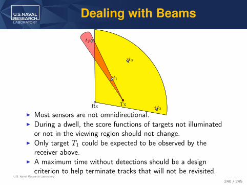
U.S. Naval Research Laboratory
Dealing with Beams
Rx Txt2
t3
t1
t2
I Most sensors are not omnidirectional.I During a dwell, the score functions of targets not illuminated
or not in the viewing region should not change.I Only target T1 could be expected to be observed by the
receiver above.I A maximum time without detections should be a design
criterion to help terminate tracks that will not be revisited.240 / 245

U.S. Naval Research Laboratory
Dealing with Beams
0◦
30◦
60◦90◦
120◦
150◦
180◦
210◦
240◦
270◦300◦
330◦
I If a target is determined to be in the transmit and receivebeams, then one will often adjust PD based on the predictedpositions in the beams and the beamshapes.
I This can be more difficult than one might expect. TheSwerling models in “MathematicalFunctions/Statistics/Detection Statistics/” in the TCL mighthelp.
241 / 245

SUMMARY
242 / 245

U.S. Naval Research Laboratory
Summary I
I Gaussian approximations and Poisson clutter are widely used.I Tracking algorithms need consistent measurement covariance
matrices. Cross terms between range and range rate canmatter.
I The Kalman filter comes from a Bayesian update of a lineardynamic model and a linear measurement.
I The EKF and CKF use Taylor series and cubatureapproximations to solve difficult integrals in an approximatenonlinear Kalman filter.
I Approaches to measurement conversion with consistentcovariances include using Taylor series and cubatureapproximations to solve difficult integrals.
243 / 245

U.S. Naval Research Laboratory
Summary II
I The GNN filter is a maximum likelihood filter for dataassociation.
I The JPDA is an MMSE (expected value) filter for dataassociation.
I One typically uses a variant of the JPDA, because theexpected value is undesirable given target identity uncertainty.
I Cascaded logic and integrated additions to GNN and JPDAfilter variants allow for track initiation and termination.
I Lots of free, commented Matlab code for tracking can befound at https://github.com/USNavalResearchLaboratory/TrackerComponentLibrary which is alsohttp://www.trackercomponentlibrary.com
244 / 245

QUESTIONS?
245 / 245