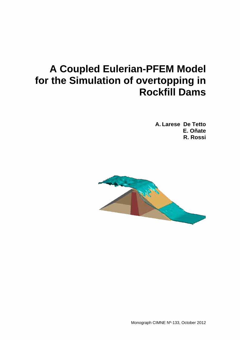
A Coupled Eulerian-PFEM Model

for the Simulation of overtopping in Rockfill Dams

A. Larese De Tetto E. Oñate R. Rossi

Monograph CIMNE Nº-133, October 2012

A Coupled Eulerian-PFEM Model for the Simulation of overtopping in

Rockfill Dams

A. Larese De Tetto E. Oñate R. Rossi

Monograph CIMNE Nº-133, October 2012

International Center for Numerical Methods in Engineering Gran Capitán s/n, 08034 Barcelona, Spain

INTERNATIONAL CENTER FOR NUMERICAL METHODS IN ENGINEERING Edificio C1, Campus Norte UPC Gran Capitán s/n 08034 Barcelona, Spain www.cimne.com First edition: October 2012 A COUPLED EULERIAN-PFEM MODEL FOR THE SIMULATION OF OVERTOPPING IN ROCKFILL DAMS Monograph CIMNE M133 The authors ISBN: 978-84-940243-6-8 Depósito legal: B-29348-2012

La losoa è s ritta in questo grandissimo libro he ontinuamente i sta apertoinnanzi a gli o hi (io di o l'universo), ma non si può intendere se prima non s'imparaa intender la lingua, e onos er i aratteri, ne' quali è s ritto. Egli è s ritto in linguamatemati a, e i aratteri son triangoli, er hi, ed altre gure geometri he, senza i qualimezzi è impossibile a intenderne umanamente parola; senza questi è un aggirarsivanamente per un os uro laberinto.Galileo Galilei, Il Saggiatore (1623)

A knowledgmentsI would like to thank all the people that are someway linked to this work and that ontribute to its realization in dierent but equally important manners.First of all I want to express my warmest gratitude to Prof. Eugenio Oñate whohas given me the possibility of developing this work, en ouraging me sin e the earlybeginning. His enthusiasm and optimism have been a strong motivating for e duringthese years. I am deeply indebted to Dr. Ri ardo Rossi whose endless patien e madepossible the realization of this monograph.In 2010 Prof. Djeordje Peri¢ gave me the opportunity to visit the College of Engineeringof Swansea University for three months. I would like to thank him for the warm wel omeand his ni e tutoring during this period. This internship gave me the possibility to meetProf. De Souza Neto, whose extreme kindness I will not forget, and Steen Bauer, agood friend.I am very grateful to all the professors of the RMEE department of the UniversitatPolitè ni a de Catalunya be ause their doors have always been opened for answeringany doubt and for any useful advi e. A really spe ial thank goes to one of them, whobelieved in me long before I even knew about believing in myself, thank you Prof. MiguelCervera.If CIMNE is a very pleasant pla e to work in, it is be ause of the people it is made of.Espe ially for all the members of o e C4, maybe the noisiest but the ni est o e of allCIMNE as well! Thank you Pooyan, Miguel Angel, Roberto, eRi ardo, Salva, Móni a,Pablo, Miquel and Ferran. They have been mu h more than simple o e mates.Thank you to all the others resear hers that are, or have been, part of CIMNE. Amongthem I would like to mention Carlos and Adelina and also Miguel, Kike, Abel, Eduardo,Kazem, Jordi, Robert.

I am very grateful to all the women of CIMNE, in parti ular to MaJesus, Mer è andLelia for their kindness and interest shown.It has been a pleasure to be involved in these years in the XPRES and EDAMS proje tswhi h gave me the possibility of starting a good ollaboration with the partners of UPMand CEDEX. I am very grateful to all of them and in parti ular to Prof. Miguel AngelToledo, Rafa Moran and Fernando Salazar. Thank you for onstantly helping me withall the physi al aspe ts of dam engineering and for sharing ni e moments during all the ongresses of dams. In this ontext I would like to mention Prof. Iñaki Es uder who gaveme the opportunity of be oming voting member of the Committee on Numeri al Aspe tsof Dams of SpanCOLD and involved me in the organization of the last Ben hmarkWorkshop on Numeri al Analysis of Dams.I am espe ially grateful to Dr. Janos h Stas heit and Prof. Umberto Perego for theiruseful advises during the revision of this do ument.During these years I have met and known a huge number of people that left me unfor-gettable memories. Some of them be ame great friends and deserve a spe ial mentionfor onstantly supporting me and sharing bad and good moments. Thank you ElisaMaria, MaCarmen, Maria Laura, Esther and Mara.When I was at the beginning of this experien e, I ould not even imagine that in spiteof the distan e, my old Italian friends would have always been so present in my life!Thank you for making me feel so loved.Last but not least I would like to thank my family: my parents Elda and Ivo and mybrother Paolo with Claudia for their endless love and my nephew Tobia who still doesnot know that this work will be ome his rst and only storybook! Finally I would liketo thank a spe ial person who has tirelessly (and not always su essfully) tried to tea hme to give the right importan e to things without falling apart after any failure: thankyou Roberto.The resear h was supported by the E-DAMS proje t of the National Plan R+D of theSpanish Ministry of S ien e and Innovation I+D BIA2010-21350-C03-00, 2010-2013.

Abstra tRo kll dams are nowadays often preferred over on rete dams be ause of their e onomi advantages, their exible design and thank to the great advan e a hieved in geos ien esand geome hani s. Unfortunately their behavior in ase of overtopping is still an openissue. In fa t very little is known on this phenomenon that in most ases leads to the omplete failure of the stru ture with atastrophi onsequen es in term of loss of livesand e onomi damage.The prin ipal aim of the present work is the development of a omputational methodto simulate the overtopping and the beginning of failure of the downstream shoulder ofa ro kll dam. The whole phenomenon is treated in a ontinuous framework.The uid free surfa e problem outside and inside the ro kll slope is treated using aunique Eulerian xed mesh formulation. A level set te hnique is employed to tra k theevolution of the free surfa e. The traditional Navier-Stokes equations are modied inorder to automati ally dete t the presen e of the porous media. The non-linear seepageis evaluated using a quadrati form of the resistan e law for whi h the Ergun's oe ientshave been hosen.The stru tural response of the solid skeleton is evaluated using a ontinuum vis ousmodel. A non-Newtonian modied Bingham law is proposed for the simulation of thebehaviour of a granular non- ohesive material. This approa h has the possibility of onsidering a pressure sensitive resistan e riterion. This is obtained inserting a Mohr-Coulomb failure riterion in the Bingham relation. Due to the large deformation of themesh during the failure pro ess, a Lagrangian framework is preferred to a xed meshone: the Parti le Finite Element Method (PFEM) is therefore used. Its spe i featuresmake it appropriate to treat the ro kll material and its large deformations and shape hanges.

Finally a tool for mapping variables between non-mat hing meshes is developed to allowpassing information between the uid xed and the dam moving meshes.All the numeri al results are ompared with experiments on prototype ro kll dams.

ResumenHoy en día las presas de es ollera resultan a menudo una ele ión preferible respeto alas tradi ionales presas de hormigón por su menor impa to e onómi o y, sobretodo, porsu mayor exibilidad de diseño gra ias a los grandes avan es al anzados en geo ien iasy en geome áni a.Sin embargo, desafortunadamente su omportamiento frente a un sobrevertido siguesiendo un aspe to des ono ido y muy difí il de analizar. Cuando el nivel de agua superala orona ión, en la mayoría de los asos se produ e la rotura ompleta de la presa on onse uen ias atastró as tanto en términos de perdida de vidas humanas omo entérminos e onómi os.El prin ipal objetivo de este trabajo es el desarrollo de un método omputa ional quepueda simular el sobrevertido y el prin ipio de la rotura del espaldón aguas abajo deuna presa de es ollera. Todo el fenómeno se trata on modelos ontinuos.El problema de ujo en super ie libre tanto fuera omo dentro de la es ollera se trata on una úni a formula ión usando un método Euleriano de malla ja y una té ni a delevel set para trazar la evolu ión de la super ie libre. Se han modi ado las lási ase ua iones de Navier-Stokes de manera que se dete te automati amente la presen iade un medio poroso. La ltra ión no lineal se evalúa mediante una ley de resisten ia uadráti a en la ual se han empleado los oe ientes de Ergun.La respuesta estru tural se evalúa usando un modelo ontinuo vis oso. Se proponeuna versión modi ada de la ley de Bingham para uidos no Newtonianos que permitesimular el omportamiento granular no ohesivo de la es ollera. La diferen ia de esteenfoque onsiste en la posibilidad de onsiderar un riterio de resisten ia que sea fun iónde la presión. Esto se obtiene insertando un riterio de fallo de Mohr Coulomb en larela ión de Bingham. Debido a las grandes deforma iones a las que se ve sometida

la malla durante el pro eso de rotura se ha preferido usar un método Lagrangianorespe to a uno de malla ja: el Métodos de Elementos Finitos y Partí ulas (PFEM). Sus ara terísti as lo ha en apropiado para simular la es ollera y sus grandes deforma ionesy ambios de forma.Finalmente se ha desarrollado una herramienta para interpolar datos entre mallas no oin identes para permitir la transferen ia de informa iones entre el modelo uido demalla ja y el modelo de la presa on malla en movimiento.Todos los resultados numéri os se han omparado on experimentos he hos sobre presasprototipo.

ContentsList of Figures VList of Tables XVIIList of Symbols XIX1 Introdu tion 11.1 Embankment dams . . . . . . . . . . . . . . . . . . . . . . . . . . . . . . 21.2 The XPRES and E-DAMS proje ts . . . . . . . . . . . . . . . . . . . . . 51.3 Obje tives . . . . . . . . . . . . . . . . . . . . . . . . . . . . . . . . . . . 71.4 Layout of the do ument . . . . . . . . . . . . . . . . . . . . . . . . . . . 82 The uid problem 112.1 Introdu tion . . . . . . . . . . . . . . . . . . . . . . . . . . . . . . . . . . 112.1.1 Flow in ro kll material . . . . . . . . . . . . . . . . . . . . . . . 122.1.2 Analogy between ow in porous media and pipes ow . . . . . . . 142.1.3 Resistan e laws . . . . . . . . . . . . . . . . . . . . . . . . . . . . 172.2 Continuous form . . . . . . . . . . . . . . . . . . . . . . . . . . . . . . . 192.2.1 Variables of the problem . . . . . . . . . . . . . . . . . . . . . . . 202.2.2 Constitutive law. Water as a Newtonian in ompressible uid . . . 202.2.3 Modied form of the Navier-Stokes equations . . . . . . . . . . . 212.3 Weak form . . . . . . . . . . . . . . . . . . . . . . . . . . . . . . . . . . . 252.4 Element-based approa h: monolithi solver . . . . . . . . . . . . . . . . . 27

II CONTENTS2.4.1 Stabilized formulation . . . . . . . . . . . . . . . . . . . . . . . . 282.4.2 Dis retization pro edure . . . . . . . . . . . . . . . . . . . . . . . 332.4.3 Bossak time integration s heme . . . . . . . . . . . . . . . . . . . 362.5 Edge-based approa h: fra tional step solver . . . . . . . . . . . . . . . . 402.5.1 Stabilized formulation . . . . . . . . . . . . . . . . . . . . . . . . 422.5.2 Dis retization pro edure . . . . . . . . . . . . . . . . . . . . . . . 442.5.3 Fra tional step solver using an expli it 4th order Runge Kutta times heme . . . . . . . . . . . . . . . . . . . . . . . . . . . . . . . . . 462.5.4 The edge-based operators . . . . . . . . . . . . . . . . . . . . . . 512.5.5 Improving mass onservation . . . . . . . . . . . . . . . . . . . . . 552.6 Free surfa e tra king. The Level Set method . . . . . . . . . . . . . . . . 562.6.1 Coupling the level set equation and the Navier-Stokes solver . . . 592.6.2 The extrapolation pro edure . . . . . . . . . . . . . . . . . . . . . 592.6.3 The distan e fun tion . . . . . . . . . . . . . . . . . . . . . . . . . 622.6.4 Pres ribing the boundary ondition on the free surfa e ∂Ωm . . 652.7 The algorithm . . . . . . . . . . . . . . . . . . . . . . . . . . . . . . . . . 682.8 Numeri al examples . . . . . . . . . . . . . . . . . . . . . . . . . . . . . . 702.8.1 Still water example . . . . . . . . . . . . . . . . . . . . . . . . . . 702.8.2 Water owing through two materials . . . . . . . . . . . . . . . . 722.8.3 Mass onservation . . . . . . . . . . . . . . . . . . . . . . . . . . . 772.8.4 Comparison of the level set algorithm with PFEM . . . . . . . . . 852.8.5 Flip bu ket . . . . . . . . . . . . . . . . . . . . . . . . . . . . . . 852.8.6 3D dambreak . . . . . . . . . . . . . . . . . . . . . . . . . . . . . 862.9 Con lusions . . . . . . . . . . . . . . . . . . . . . . . . . . . . . . . . . . 943 The stru tural problem 973.1 Introdu tion . . . . . . . . . . . . . . . . . . . . . . . . . . . . . . . . . . 973.2 Stru tural onstitutive law. An overview of non-Newtonian models . . . . 993.2.1 Constant yield: the Bingham model . . . . . . . . . . . . . . . . . 1013.2.2 Variable yield vis o-rigid model . . . . . . . . . . . . . . . . . . . 1043.3 Continuous form . . . . . . . . . . . . . . . . . . . . . . . . . . . . . . . 1053.3.1 Variables of the problem . . . . . . . . . . . . . . . . . . . . . . . 1053.3.2 Balan e equations . . . . . . . . . . . . . . . . . . . . . . . . . . . 106

CONTENTS III3.4 Weak form . . . . . . . . . . . . . . . . . . . . . . . . . . . . . . . . . . . 1073.5 The stru tural approa h: monolithi solver . . . . . . . . . . . . . . . . . 1083.5.1 Stabilized formulation . . . . . . . . . . . . . . . . . . . . . . . . 1083.5.2 Dis retization pro edure . . . . . . . . . . . . . . . . . . . . . . . 1093.5.3 Bossak time integration s heme . . . . . . . . . . . . . . . . . . . 1093.6 Kinemati framework of the non-Newtonian stru tural element . . . . . . 1123.7 The parti le nite element method (PFEM) . . . . . . . . . . . . . . . . 1133.7.1 Updated Lagrangian kinemati al des ription of motion . . . . . . 1143.7.2 Remeshing algorithm . . . . . . . . . . . . . . . . . . . . . . . . . 1153.7.3 Boundary re ognition method: alpha - shape method . . . . . . . 1153.7.4 FEM . . . . . . . . . . . . . . . . . . . . . . . . . . . . . . . . . . 1163.7.5 PFEM algorithm . . . . . . . . . . . . . . . . . . . . . . . . . . . 1173.8 Numeri al Examples . . . . . . . . . . . . . . . . . . . . . . . . . . . . . 1173.8.1 The Couette ow . . . . . . . . . . . . . . . . . . . . . . . . . . . 1173.8.2 Cavity ow . . . . . . . . . . . . . . . . . . . . . . . . . . . . . . 1213.8.3 Extrusion pro ess . . . . . . . . . . . . . . . . . . . . . . . . . . . 1263.8.4 Bingham vs variable vis osity model. Pushed slope . . . . . . . . 1283.8.5 Settlement of a verti al ro kll slope . . . . . . . . . . . . . . . . 1373.8.6 Fri tion angle test . . . . . . . . . . . . . . . . . . . . . . . . . . . 1403.9 Con lusions . . . . . . . . . . . . . . . . . . . . . . . . . . . . . . . . . . 1434 The oupling 1454.1 Introdu tion . . . . . . . . . . . . . . . . . . . . . . . . . . . . . . . . . . 1454.2 The oupled monolithi problem . . . . . . . . . . . . . . . . . . . . . . . 1474.3 The uid and the stru tural balan e equations . . . . . . . . . . . . . . 1474.4 The oupling strategy . . . . . . . . . . . . . . . . . . . . . . . . . . . . . 1494.4.1 Numeri al Example: Still water tank . . . . . . . . . . . . . . . . 1514.5 Data mapping between non-mat hing meshes . . . . . . . . . . . . . . . . 1554.5.1 The sear hing algorithm . . . . . . . . . . . . . . . . . . . . . . . 1584.5.2 Numeri al Examples . . . . . . . . . . . . . . . . . . . . . . . . . 1614.6 Con lusions . . . . . . . . . . . . . . . . . . . . . . . . . . . . . . . . . . 1655 Failure analysis of s ale models of ro kll dams under seepage ondi-

IV CONTENTStions 1675.1 Introdu tion . . . . . . . . . . . . . . . . . . . . . . . . . . . . . . . . . . 1675.2 Overview of the ase study . . . . . . . . . . . . . . . . . . . . . . . . . . 1715.3 CASE A: Homogeneous dam . . . . . . . . . . . . . . . . . . . . . . . . . 1745.3.1 Case A. Experimental setting and geometry . . . . . . . . . . . . 1745.3.2 Case A1. 2D numeri al model and results . . . . . . . . . . . . 1755.3.3 Case A1. Mesh inuen e . . . . . . . . . . . . . . . . . . . . . . . 1775.3.4 Case A1. Inuen e of porosity . . . . . . . . . . . . . . . . . . . . 1775.3.5 Case A1. Inuen e of the diameter of the material . . . . . . . . . 1795.3.6 Case A1. 3D numeri al model and results . . . . . . . . . . . . 1805.3.7 Case A2. 2D oupled model and results . . . . . . . . . . . . . 1835.3.8 Case A2. 2D sequen e of in remental dis harges . . . . . . . . . 1875.3.9 Case A2. 3D oupled model and results . . . . . . . . . . . . . 1885.4 CASE B. Core dam . . . . . . . . . . . . . . . . . . . . . . . . . . . . . . 1905.4.1 Case B. Core dam. Experimental setting and geometry . . . . . . 1915.4.2 Case B1a. Core dam. 2D numeri al model and results . . . . . 1925.4.3 Cases B1b and B1 . Core dam. Comparison with theoreti alErgun model . . . . . . . . . . . . . . . . . . . . . . . . . . . . . 1935.4.4 Case B1a. Core dam. 3D numeri al model and results . . . . . 1945.4.5 Case B2. Core dam. Coupled model and results . . . . . . . . . . 1965.4.6 Case B21. Core dam. Sensitivity analysis: internal fri tion angle . 1985.4.7 Case B2 with φ = 41 . . . . . . . . . . . . . . . . . . . . . . . . . 1995.5 CASE C. Impervious fa e dam . . . . . . . . . . . . . . . . . . . . . . . . 2025.5.1 Case C. Impervious fa e dam. Experimental setting and geometry 2035.5.2 Case C1. Impervious fa e dam. Un oupled model and results . . 2045.5.3 Case C2. Impervious fa e dam. Coupled model and results . . . . 2065.6 Con lusions and future work . . . . . . . . . . . . . . . . . . . . . . . . . 2106 Con lusions 2136.1 Summary and a hievements . . . . . . . . . . . . . . . . . . . . . . . . . 2136.2 Future lines of resear h . . . . . . . . . . . . . . . . . . . . . . . . . . . . 214A Kratos Multiphysi s 217

CONTENTS VA.1 Kratos . . . . . . . . . . . . . . . . . . . . . . . . . . . . . . . . . . . . . 217A.1.1 Obje t-oriented approa h . . . . . . . . . . . . . . . . . . . . . . 217A.1.2 Multi- layer design . . . . . . . . . . . . . . . . . . . . . . . . . . 218A.1.3 Python interfa e . . . . . . . . . . . . . . . . . . . . . . . . . . . 220A.2 GiD problem types and interfa es . . . . . . . . . . . . . . . . . . . . . . 220

VI CONTENTS

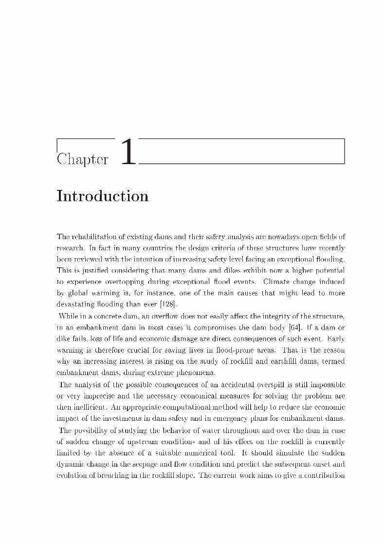
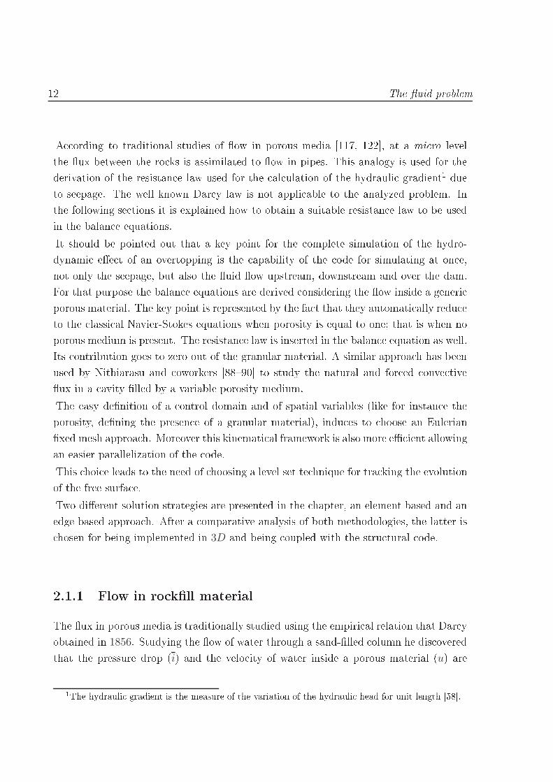
List of Figures1.1 Image of Banqiao dam. Image taken from [1. . . . . . . . . . . . . . . . 31.2 Image of Tous dam after the overtopping of O tober 19th, 1982. . . . . . 31.3 Glashütte embankment dam (Germany). Image taken from [30. . . . . . 41.4 The images show two experiments arried out at the UPM laboratories.On the left an example of mass sliding failure (initial slope 1V : 1.5H)whereas on the right the failure is mainly due to super ial dragging ofparti les (initial slope 1V : 3H). . . . . . . . . . . . . . . . . . . . . . . 51.5 S hemati ross se tion of a ro kll dam. . . . . . . . . . . . . . . . . . . 51.6 UPM and CEDEX experimental hannels used for XPRES and E-DAMSproje ts. . . . . . . . . . . . . . . . . . . . . . . . . . . . . . . . . . . . . 62.1 Graphi al des ription of uid velo ity u (averaged over the empty volume

ΩE) and Dar y velo ity u (averaged over the total ontrol volume Ω). . 142.2 Range of validity of Dar y law in its linear form. . . . . . . . . . . . . . . 172.3 Balan e of onservation of mass in a dis rete volume dx dy. dxdy =

n dx dy is the empty volume where the uid an ir ulate. . . . . . . . . 222.4 Balan e of onservation of linear momentum in a dis rete volume dx dy.dxdy = n dx dy is the empty volume where the uid an ir ulate. . . . . 232.5 Denition of elemental porosity with a dominant porosity riteria. . . . . 282.6 Build up ontribution in an edge-based data stru ture for the elemental ontribution. . . . . . . . . . . . . . . . . . . . . . . . . . . . . . . . . . . 412.7 Graphi representation of the level set fun tion ϕ. . . . . . . . . . . . . . 572.8 Extrapolation layers and al ulated nodes in the time interval tn − tn+1. . 60

VIII LIST OF FIGURES2.9 Cal ulation of nodal distan es di on the nodes i of one element ut by thefree surfa e. . . . . . . . . . . . . . . . . . . . . . . . . . . . . . . . . . . 642.10 Splitting pro edure for the elements ut by the free surfa e. . . . . . . . . 662.11 Graphi al explanation of the evaluation of pressure on the rst layer ofnon uid nodes in order to respe t the in ompressibility ondition. . . . 672.12 Geometry, stru tured mesh and onditions of the still water model. . . . 712.13 Pressure distribution. . . . . . . . . . . . . . . . . . . . . . . . . . . . . . 712.14 Pressure distribution in a verti al se tion. Comparison between the twoalgorithms. . . . . . . . . . . . . . . . . . . . . . . . . . . . . . . . . . . 722.15 Geometry, stru tured mesh and onditions of the two material model withbottom in oming water. . . . . . . . . . . . . . . . . . . . . . . . . . . . 732.16 Evolution of free surfa e for both algorithms. . . . . . . . . . . . . . . . . 742.17 Pressure distribution when water level rea hes 2.5m from the bottom. . . 752.18 Pressure distribution when water level rea hes the top. . . . . . . . . . . 762.19 Geometry, mesh and onditions of the mass onservation model. . . . . 772.20 2D Verti al olumn. Element-based algorithm. Evolution of free surfa eat 10− 20− 30− 40− 50 sec. . . . . . . . . . . . . . . . . . . . . . . . . 782.21 2D Verti al olumn. Edge-based algorithm. Evolution of free surfa e at10-20-30-40-50 se . . . . . . . . . . . . . . . . . . . . . . . . . . . . . . . 792.22 3D verti al olumn. Geometry and mesh taken into a ount. . . . . . . 812.23 3D verti al olumn. Stru tured medium mesh. Evolution of free surfa efor 1m/s bottom in oming velo ity. On the right of ea h snapshot theexpe ted level is indi ated. . . . . . . . . . . . . . . . . . . . . . . . . . . 812.24 3D verti al olumn. Unstru tured medium mesh. Evolution of free sur-fa e for 1m/s bottom in oming velo ity. On the right of ea h snapshotthe expe ted level is indi ated. . . . . . . . . . . . . . . . . . . . . . . . . 822.25 Mesh and geometry of the verti al hannel with lateral entran e of water 822.26 Verti al olumn with lateral entran e example. Level of water in termsof time. . . . . . . . . . . . . . . . . . . . . . . . . . . . . . . . . . . . . 832.27 Verti al olumn with lateral entran e example. Evolution of the freesurfa e at 50s, 120s, and 230s. . . . . . . . . . . . . . . . . . . . . . . . . 842.28 Geometry and boundary ondition of the ip bu ket example. . . . . . . 852.29 Mesh of the ip bu ket example. . . . . . . . . . . . . . . . . . . . . . . . 85

LIST OF FIGURES IX2.30 Sequen e of the transitory phase of the jet. . . . . . . . . . . . . . . . . . 862.31 Level set and PFEM omparisons in the pressure head al ulation andthe jet development . . . . . . . . . . . . . . . . . . . . . . . . . . . . . . 872.32 Geometry and boundary ondition of the 3D dam break example. Onthe lower left orner a zoom on the pressure sensors distribution on thestep . . . . . . . . . . . . . . . . . . . . . . . . . . . . . . . . . . . . . . 882.33 The two meshes onsidered. On the left Mesh A of 296 157 and Mesh Bof 2 310 984 tetrahedra. . . . . . . . . . . . . . . . . . . . . . . . . . . . . 892.34 Evolution of the dam break at 0.4s, 0.6s and 2.0s. Comparison betweenthe results obtained with meshes A and B. . . . . . . . . . . . . . . . . . 892.35 Pressure evolution on P1 on the verti al fa e of the step indi ated inFigure 2.32. Comparison of level set, PFEM and experimental results. . . 902.36 Pressure evolution on P2 on the verti al fa e of the step indi ated in Fig.2.32. Comparison of level set, PFEM and experimental results. . . . . . . 912.37 Pressure evolution on P3 on the verti al fa e of the step indi ated in Fig.2.32. Comparison of level set, PFEM and experimental results. . . . . . . 912.38 Pressure evolution on P4 on the verti al fa e of the step indi ated in Fig.2.32. Comparison of level set, PFEM and experimental results. . . . . . . 922.39 Pressure evolution on P5 on the top fa e of the step indi ated in Fig.2.32. Comparison of level set, PFEM and experimental results. . . . . . . 922.40 Pressure evolution on P6 on the top fa e of the step indi ated in Fig.2.32. Comparison of level set, PFEM and experimental results. . . . . . . 932.41 Pressure evolution on P7 on the top fa e of the step indi ated in Fig.2.32. Comparison of level set, PFEM and experimental results. . . . . . . 932.42 Pressure evolution on P8 on the top fa e of the step indi ated in Fig.2.32. Comparison of level set, PFEM and experimental results. . . . . . . 943.1 Qualitative ow urves for the dierent ategories of non-Newtonian uids.1013.2 Comparison between a Newtonian uid and a Bingham uid behaviorwith a yield stress τ0. . . . . . . . . . . . . . . . . . . . . . . . . . . . . . 1023.3 Newtonian and Bingham uid ompared with the regularized model forin reasing values of the m parameter. . . . . . . . . . . . . . . . . . . . . 1033.4 Possible boundaries of a loud of nodes using alpha shapes method. Imagetaken from [20. . . . . . . . . . . . . . . . . . . . . . . . . . . . . . . . . 116

X LIST OF FIGURES3.5 Geometri al data and boundary onditions. . . . . . . . . . . . . . . . . 1183.6 Linear triangular mesh used in the al ulation. . . . . . . . . . . . . . . 1183.7 Exponential approximation with m=300 and τ0 = 100Pa. . . . . . . . . . 1193.8 Variation f vis osity in the entral verti al se tion. . . . . . . . . . . . . . 1193.9 Velo ity diagrams for dierent values of the gradient of pressure. Upperhorizontal velo ity 0.5m/s. . . . . . . . . . . . . . . . . . . . . . . . . . . 1203.10 Velo ity diagrams for dierent values of a negative gradient of pressure.Upper horizontal velo ity 0.01m/s. . . . . . . . . . . . . . . . . . . . . . 1203.11 Cavity example. Meshes used in the al ulation. . . . . . . . . . . . . . . 1213.12 Cavity. White olor shows the yielded regions. Comparison between the ase with homogeneous mesh (Figure 3.11(a)) and the rened one (Figure3.11(b)). . . . . . . . . . . . . . . . . . . . . . . . . . . . . . . . . . . . . 1223.13 Cavity. White olor shows the yielded regions. Comparison between the ase with homogeneous mesh (gure 3.11(a)) and the rened one (gure3.11(b)). . . . . . . . . . . . . . . . . . . . . . . . . . . . . . . . . . . . . 1233.14 Cavity example. Streamlines and progressive evolution of the yielded area(white olor) for in reasing values of the Bingham number Bn (Bn = 2, 20and 200 respe tively). . . . . . . . . . . . . . . . . . . . . . . . . . . . . . 1243.15 Cavity example. Streamlines and progressive evolution of the yielded area(white olor) for in reasing values of the Bingham number Bn (Bn = 5, 50and 500 respe tively). . . . . . . . . . . . . . . . . . . . . . . . . . . . . . 1253.16 Extrusion example. Ramp fun tion of external pressure BC applied onleft verti al side. . . . . . . . . . . . . . . . . . . . . . . . . . . . . . . . 1263.17 Extrusion example. Geometry and boundary onditions. . . . . . . . . . 1273.18 Extrusion example. Mesh used in the al ulation. Average dimensionh = 0.2m with a lo al renement 0.05m near point B of Figure 3.17 andin the restri tion area and an additional renement 0.005m lose to pointA of Figure 3.17. The total number of triangular elements and nodes are11 600 and 5 800, respe tively. . . . . . . . . . . . . . . . . . . . . . . . . 1273.19 Extrusion example. Evolution of the slip lines shown with a ontour llof the equivalent strain rate γ. Comparison between the present model(left olumn) and the results presented in [105 (right olumn). . . . . . . 129

LIST OF FIGURES XI3.20 Extrusion example. Evolution of the slip lines shown with a ontour llof the equivalent strain rate γ. Comparison between the present model(left olumn) and the results presented in [105 (right olumn). . . . . . . 1303.21 Extrusion example. Pressure-velo ity relationship on point B. . . . . . . 1313.22 Pushed slope example. Geometry, mesh and boundary onditions of 2Dand 3D models. . . . . . . . . . . . . . . . . . . . . . . . . . . . . . . . . 1313.23 2D pushed slope. γ in the initial pushing phase. Dieren e between theBingham and the variable vis osity models. . . . . . . . . . . . . . . . . . 1333.24 2D pushed slope. γ in the squeezing phase. Dieren e between theBingham and the variable vis osity models. . . . . . . . . . . . . . . . . . 1343.25 3D pushed slope. Dieren e between the Bingham and the variable vis- osity models in the initial pushing phase. . . . . . . . . . . . . . . . . . 1353.26 3D pushed slope. Dieren e between the Bingham and the variable vis- osity models in the squeezing phase. . . . . . . . . . . . . . . . . . . . . 1363.27 Settlement of a verti al slope. Geometry of the model. . . . . . . . . . . 1373.28 Dierent mesh sizes taken into a ount in the present example. . . . . . 1383.29 Settlements for a granular slope with internal fri tion angle φ = 30 forthe three dierent mesh sizes indi ated in Figure 3.28. . . . . . . . . . . . 1393.30 Dierent results of the model with phi = 45 in ase of mesh B (0.05m)and a oarser mesh (0.07m). Both results are taken after 5s of simulation. 1403.31 Settlements for a 3D granular slope with internal fri tion angle φ = 30in the ase of onsidering mesh A and B of Figure 3.28. . . . . . . . . . . 1413.32 Stable results for dierent internal fri tion angles φ. The mesh used inthe al ulation is mesh B of Figure 3.28. . . . . . . . . . . . . . . . . . . 1423.33 Fri tion angle test example. Geometry and mesh used for the al ulation. 1433.34 Fri tion angle test example. Variable yield model with ϕ = 40. . . . . . 1433.35 Fri tion angle test example. Bingham model with yield stress τ0 = 500Pa. 1444.1 Graphi al summary of the whole pro ess. . . . . . . . . . . . . . . . . . 1494.2 Geometry of the tank and height of the ontained porous medium. . . . . 1514.3 Depth of water in the three analyzed ases. . . . . . . . . . . . . . . . . . 1524.4 Case A. hfA = 0.25m Ee tive Pressure p′

s. . . . . . . . . . . . . . . . . . 1544.5 Case B. hfB = 0.50m Ee tive Pressure p′

s. . . . . . . . . . . . . . . . . . 154

XII LIST OF FIGURES4.6 Case C. hfC = 0.75m Ee tive Pressure p′

s. . . . . . . . . . . . . . . . . . 1554.7 2D example of the interpolation pro edure. Node I, J and K are insidethe ir ums ribed ir le but only node J in inside the element and itsvalue of alpha an be al ulated. . . . . . . . . . . . . . . . . . . . . . . . 1574.8 S hemati representation of a k-d tree data stru ture taken from [69. . . 1594.9 Representation of a k-d tree partitioning taken from [47. . . . . . . . . . 1594.10 Representation of a bins partitioning taken from [47. . . . . . . . . . . . 1604.11 Bins stru ture taken from [47. . . . . . . . . . . . . . 1604.12 Meshes used in the al ulation whose element dimension is reported inTable4.3. Left: Lagrangian (PFEM) mesh and right: Eulerian xed mesh. 1614.13 Mapping between models with Mesh A. . . . . . . . . . . . . . . . . . . . 1634.14 Mapping between models with Mesh B. . . . . . . . . . . . . . . . . . . . 1634.15 Mapping from a ne mesh (mesh A) to a oarse one (mesh B). . . . . . . 1644.16 Comparison between the performan e of k-d tree, bins, and k-d tree ofbins data stru tures for the proje tion of a s alar variable for dierentmesh sizes. . . . . . . . . . . . . . . . . . . . . . . . . . . . . . . . . . . . 1655.1 Pressure instrumentation. . . . . . . . . . . . . . . . . . . . . . . . . . . 1685.2 Length of failure. Chara terization and operative measurement. . . . . . 1695.3 Length of failure. Digital model of the deformed slope to evaluate theevolution of failure B. . . . . . . . . . . . . . . . . . . . . . . . . . . . . 1695.4 Granulometri analysis of ro kll material a ording to the UNE-EN 933-1.1725.5 Experimental setting. . . . . . . . . . . . . . . . . . . . . . . . . . . . . . 1745.6 Case A. Geometry of the experimental setting and map of the sensorsdistribution. . . . . . . . . . . . . . . . . . . . . . . . . . . . . . . . . . . 1745.7 Case A1. Qualitative model geometry and boundary onditions . . . . . 1755.8 Case A1. Evolution of the seepage line in a dam with porosity n = 0.4and D50 = 35mm. Q = 25, 46l/s. . . . . . . . . . . . . . . . . . . . . . . 1765.9 Case A1. Bottom pressure distribution at stationary regime for Q =

25, 46l/s. Porosity n = 0.4, D50 = 35mm. Numeri al and experimental omparison. . . . . . . . . . . . . . . . . . . . . . . . . . . . . . . . . . . 1765.10 Case A1. Meshes used in the analysis of mesh sensitivity. Detailed har-a teristi s of the meshes an be found in Table 5.3. . . . . . . . . . . . . 178

LIST OF FIGURES XIII5.11 Case A1. Inuen e of the mesh. . . . . . . . . . . . . . . . . . . . . . . . 1785.12 Case A1. Pressure head distribution for porosity n = 0.3, 0.35, 0.4 and 0.45.1785.13 Case A1. Zoom of the pressure head distribution for porosity n =

0.37, 0.38 and 0.39. . . . . . . . . . . . . . . . . . . . . . . . . . . . . . . 1795.14 Case A1. Inuen e of the diameter of the material. . . . . . . . . . . . . 1795.15 Case A1. 3D model and mesh. . . . . . . . . . . . . . . . . . . . . . . . . 1805.16 Case A1 3D. Evolution of the seepage line in a dam with porosity n = 0.4and D50 = 35mm. Q = 25, 46l/s. . . . . . . . . . . . . . . . . . . . . . . 1805.17 Case A1 (3D). Bottom pressure distribution at stationary regime alongthe three sensors lines (Y = 0.04m, 1.23m, 2.42m respe tively) for Q =

25, 46l/s. Porosity n = 0.4, D50 = 35mm. Numeri al and experimental omparison. . . . . . . . . . . . . . . . . . . . . . . . . . . . . . . . . . . 1815.18 Case A1. Bottom pressure distribution in 2D and in 3D models at dier-ent instan es of the transitory regime. Q = 25.46l/s. Porosity n = 0.4,D50 = 35mm. . . . . . . . . . . . . . . . . . . . . . . . . . . . . . . . . . 1825.19 Case A2. Fluid and dam qualitative models and boundary onditions forthe oupled analysis. . . . . . . . . . . . . . . . . . . . . . . . . . . . . . 1835.20 Case A2. 2D mesh of the dam model. 3.400 linear triangular elements. . 1845.21 Case A21. 2D omparison between experimental and numeri al length offailure. . . . . . . . . . . . . . . . . . . . . . . . . . . . . . . . . . . . . . 1855.22 Case A22. 2D omparison between experimental and numeri al length offailure. . . . . . . . . . . . . . . . . . . . . . . . . . . . . . . . . . . . . . 1855.23 Case A23. 2D omparison between experimental and numeri al length offailure. . . . . . . . . . . . . . . . . . . . . . . . . . . . . . . . . . . . . . 1865.24 Case A21. Bottom pressure distribution at stationary regime for Q =

51.75l/s. Porosity n = 0.4, D50 = 35mm. Numeri al and experimental omparison. . . . . . . . . . . . . . . . . . . . . . . . . . . . . . . . . . . 1865.25 Case A22. Bottom pressure distribution at stationary regime for Q =

69.07l/s. Porosity n = 0.4, D50 = 35mm. Numeri al and experimental omparison. . . . . . . . . . . . . . . . . . . . . . . . . . . . . . . . . . . 1875.26 Case A23. Bottom pressure distribution at stationary regime for Q =

90.68l/s. Porosity n = 0.4, D50 = 35mm. Numeri al and experimental omparison. . . . . . . . . . . . . . . . . . . . . . . . . . . . . . . . . . . 187

XIV LIST OF FIGURES5.27 Imposed in oming dis harge in fun tion of time. . . . . . . . . . . . . . . 1885.28 Bottom pressure distribution onsidering the hydrogram presented in Fig-ure 5.27. Porosity n = 0.4, D50 = 35mm. Numeri al and experimental omparison. . . . . . . . . . . . . . . . . . . . . . . . . . . . . . . . . . . 1895.29 Case A22 3D. Numeri al and experimental length of failure. . . . . . . . 1895.30 Case A22 3D. Bottom pressure distribution at stationary regime forQ = 69.07l/s. Porosity n = 0.4, D50 = 35mm. 2D and 3D numeri alresults ompared with experimental data points. . . . . . . . . . . . . . . 1905.31 Core dam. Experimental setting. . . . . . . . . . . . . . . . . . . . . . . 1905.32 Case B. Geometry of the experimental setting and map of the sensorsdistribution. . . . . . . . . . . . . . . . . . . . . . . . . . . . . . . . . . . 1915.33 Case B1. Qualitative model geometry and boundary onditions. . . . . . 1915.34 Case B1a. Mesh used in the al ulation. . . . . . . . . . . . . . . . . . . 1925.35 Case B1a. Bottom pressure distribution at stationary regime for Q =

5.93l/s. Porosity n = 0.4, D50 = 35mm. Numeri al and experimental omparison. . . . . . . . . . . . . . . . . . . . . . . . . . . . . . . . . . . 1925.36 Case B1(b- ).Mesh used in the al ulation. . . . . . . . . . . . . . . . . . 1935.37 Case B1b. Bottom pressure distribution at stationary regime for Q =

4.0l/s. Porosity n = 0.4, D50 = 35mm. Numeri al, experimental andtheoreti al omparison. . . . . . . . . . . . . . . . . . . . . . . . . . . . . 1945.38 Case B1b. Bottom pressure distribution at stationary regime for Q =

16.7l/s. Porosity n = 0.4, D50 = 35mm. Numeri al, experimental andtheoreti al omparison. . . . . . . . . . . . . . . . . . . . . . . . . . . . . 1945.39 Case B1a 3D. Evolution of the seepage line in a dam with porosityn = 0.4 and D50 = 35mm. Q = 5.93l/s. . . . . . . . . . . . . . . . . . . . 1955.40 Case A1. Meshes used in the analysis of mesh sensitivity. The hara ter-isti s of the meshes an be found in Table 5.6. . . . . . . . . . . . . . . . 1965.41 Case B1a (3D). Bottom pressure distribution at stationary regime forQ = 5.93l/s. Porosity n = 0.4, D50 = 35mm. Numeri al, experimentaland theoreti al omparison. . . . . . . . . . . . . . . . . . . . . . . . . . 1975.42 Case B2. Fluid and dam qualitative models and boundary onditions forthe oupled analysis. . . . . . . . . . . . . . . . . . . . . . . . . . . . . . 1975.43 Case B2. 2D mesh of the dam model. 8 000 linear triangular elements. . 198

LIST OF FIGURES XV5.44 Case B21. Bottom pressure distribution at stationary regime for Q =

19.36l/s. Porosity n = 0.4, D50 = 35mm. Numeri al and experimental omparison for dierent internal fri tion angles φ. . . . . . . . . . . . . . 1995.45 Case B21. 2D omparison between experimental and numeri al length offailure. . . . . . . . . . . . . . . . . . . . . . . . . . . . . . . . . . . . . . 2005.46 Case B22. 2D omparison between experimental and numeri al length offailure. . . . . . . . . . . . . . . . . . . . . . . . . . . . . . . . . . . . . . 2005.47 Case B23. 2D omparison between experimental and numeri al length offailure. . . . . . . . . . . . . . . . . . . . . . . . . . . . . . . . . . . . . . 2005.48 Case B21. Bottom pressure distribution at stationary regime for Q =

19.36l/s. Porosity n = 0.4, D50 = 35mm. Numeri al and experimental omparison. . . . . . . . . . . . . . . . . . . . . . . . . . . . . . . . . . . 2015.49 Case B22. Bottom pressure distribution at stationary regime for Q =

30.45l/s. Porosity n = 0.4, D50 = 35mm. Numeri al and experimental omparison. . . . . . . . . . . . . . . . . . . . . . . . . . . . . . . . . . . 2015.50 Case B23. Bottom pressure distribution at stationary regime for Q =

39.56l/s. Porosity n = 0.4, D50 = 35mm. Numeri al and experimental omparison. . . . . . . . . . . . . . . . . . . . . . . . . . . . . . . . . . . 2025.51 Case C1. Experimental setting. . . . . . . . . . . . . . . . . . . . . . . . 2025.52 Case C1. Impervious fa e dam. Geometry of the experimental settingand map of the sensors distribution. . . . . . . . . . . . . . . . . . . . . . 2035.53 Impervious fa e dam. Qualitative model geometry and boundary ondi-tions. . . . . . . . . . . . . . . . . . . . . . . . . . . . . . . . . . . . . . . 2045.54 Case C1. Meshes used in the analysis of mesh sensitivity. Detailed har-a teristi s of the meshes an be found in Table 5.9. . . . . . . . . . . . . 2055.55 Case C1. Steady state onguration in C1 ase with mesh A an Drespe tively. The blue line represents the free surfa e. . . . . . . . . . . . 2055.56 Case C. Bottom pressure distribution at stationary regime forQ = 5.17l/s.Porosity n = 0.4, D50 = 35mm. Numeri al and experimental omparisonfor the dierent meshes analyzed. . . . . . . . . . . . . . . . . . . . . . . 2065.57 Case C2. Fluid and dam qualitative models and boundary onditions forthe oupled analysis. . . . . . . . . . . . . . . . . . . . . . . . . . . . . . 2065.58 Case C2. 2D mesh of the dam model. 9.400 linear triangular elements. . 207

XVI LIST OF FIGURES5.59 Case C21. 2D omparison between experimental and numeri al length offailure. . . . . . . . . . . . . . . . . . . . . . . . . . . . . . . . . . . . . . 2075.60 Case C22. 2D omparison between experimental and numeri al length offailure. . . . . . . . . . . . . . . . . . . . . . . . . . . . . . . . . . . . . . 2085.61 Case C23. 2D omparison between experimental and numeri al length offailure. . . . . . . . . . . . . . . . . . . . . . . . . . . . . . . . . . . . . . 2085.62 Case C21. Bottom pressure distribution at stationary regime for Q =

39.56l/s. Porosity n = 0.4, D50 = 35mm. Numeri al and experimental omparison. . . . . . . . . . . . . . . . . . . . . . . . . . . . . . . . . . . 2095.63 Case C22. Bottom pressure distribution at stationary regime for Q =

39.56l/s. Porosity n = 0.4, D50 = 35mm. Numeri al and experimental omparison. . . . . . . . . . . . . . . . . . . . . . . . . . . . . . . . . . . 2095.64 Case C23. Bottom pressure distribution at stationary regime for Q =

39.56l/s. Porosity n = 0.4, D50 = 35mm. Numeri al and experimental omparison. . . . . . . . . . . . . . . . . . . . . . . . . . . . . . . . . . . 209A.1 List of the prin ipal obje t in Kratos. Image taken from [47. . . . . . . . 218A.2 Graphi al summary of the multi.layer design. Image taken from [47. . . 219

List of Tables2.1 Stabilizing elemental terms in the ASGS method. . . . . . . . . . . . . . 322.2 Matri es and ve tors of system 2.48 without stabilization terms. . . . . . 342.3 Stabilization matri es and ve tors of system 2.48. . . . . . . . . . . . . . 352.4 Matri es and ve tors of the semi dis rete form of equations 2.75. . . . . . 452.5 Stabilization matri es and ve tors of system 2.75. . . . . . . . . . . . . . 452.6 3D verti al olumn. Number of nodes, number of elements, elementallength (unstru tured meshes) and number of elements per edge (stru -tured mesh) of the meshes onsidered in the analysis. . . . . . . . . . . 802.7 Verti al olumn with lateral entran e example. Number of nodes andnumber of elements for the meshes onsidered in the analysis. . . . . . . 832.8 Dam break example. Number of nodes and number of elements of thetwo meshes onsidered in the analysis. . . . . . . . . . . . . . . . . . . . 883.1 Stabilizing elemental terms in ASGS for the non-Newtonian element. . . 1093.2 Matri es and ve tors of system 3.24 without stabilization terms. . . . . . 1103.3 Stabilization matri es and ve tors of system 3.24. . . . . . . . . . . . . . 1113.4 Couette example. Material properties. . . . . . . . . . . . . . . . . . . . 1183.5 Extrusion example. Material properties. . . . . . . . . . . . . . . . . . . 1283.6 Pushed slope example. Material properties. . . . . . . . . . . . . . . . . 1323.7 Settlement example. Material properties. . . . . . . . . . . . . . . . . . 1373.8 Fri tion angle test example. Material properties. . . . . . . . . . . . . . 1424.1 Chara teristi s of the materials onsidered in the model. . . . . . . . . . 152

XVIII LIST OF TABLES4.2 Ee tive pressure at the bottom. . . . . . . . . . . . . . . . . . . . . . . 1534.3 Size of the two meshes onsidered in the proje tion example. . . . . . . 1624.4 Mesh dimension of the four meshes onsidered in the proje tion example.The last two rows indi ates the number of nodes and elements for theEulerian destination mesh (Eul) and the Lagrangian origin one (Lagr). . 1645.1 Properties of ro kll material. . . . . . . . . . . . . . . . . . . . . . . . 1715.2 Case study. . . . . . . . . . . . . . . . . . . . . . . . . . . . . . . . . . . 1735.3 Case A1. Mesh sizes used in the mesh sensitivity study. . . . . . . . . . 1775.4 A tivated sensors lines in ase A. . . . . . . . . . . . . . . . . . . . . . . 1815.5 Case A2. Comparison between experimental (Bexp) and numeri al (Bnum)length of failure. . . . . . . . . . . . . . . . . . . . . . . . . . . . . . . . 1865.6 Case B1a. Meshes used for the analysis. . . . . . . . . . . . . . . . . . . 1955.7 Case B21. Length of failure B for dierent φ. . . . . . . . . . . . . . . . 1985.8 Case B2. Comparison between experimental (Bexp) and numeri al (Bnum)length of failure for φ = 41. . . . . . . . . . . . . . . . . . . . . . . . . 2015.9 Case C1. Meshes used in the analysis. . . . . . . . . . . . . . . . . . . . 2045.10 Case C2. Comparison between experimental (Bexp) and numeri al (Bnum)length of failure. . . . . . . . . . . . . . . . . . . . . . . . . . . . . . . . 208

List of Symbolsu : uid Dar y velo ity;u : uid velo ity;us : stru tural velo ity;uC : oupled velo ity;uM : mesh velo ity;ug : uid Dar y velo ity on the Gauss point;ug : uid velo ity on the Gauss point;p : uid pressure;ps : solid total pressure;p′s : solid ee tive pressure;pC : oupled pressure;v : ve tor of unknowns;x : ve tor of uid displa ements;xs : ve tor of solid displa ements;σ : stress tensor;τ : deviatori part of the stress tensor;ε : rate of strain tensor;τ0 : yield stress;γ : equivalent strain rate;φ : internal fri tion angle;n : porosity;n : external normal ve tor;

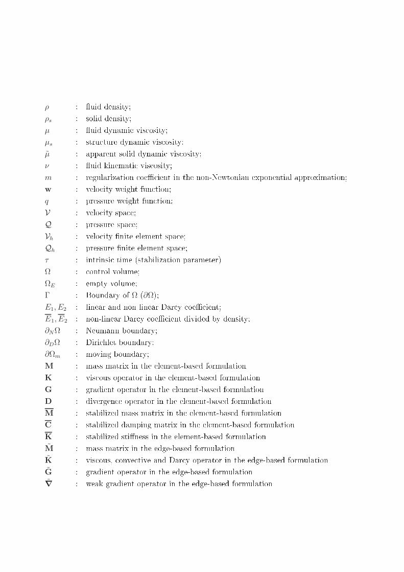
ρ : uid density;ρs : solid density;µ : uid dynami vis osity;µs : stru ture dynami vis osity;µ : apparent solid dynami vis osity;ν : uid kinemati vis osity;m : regularization oe ient in the non-Newtonian exponential approximation;w : velo ity weight fun tion;q : pressure weight fun tion;V : velo ity spa e;Q : pressure spa e;Vh : velo ity nite element spa e;Qh : pressure nite element spa e;τ : intrinsi time (stabilization parameter)Ω : ontrol volume;ΩE : empty volume;Γ : Boundary of Ω (∂Ω);E1, E2 : linear and non linear Dar y oe ient;E1, E2 : non-linear Dar y oe ient divided by density;∂NΩ : Neumann boundary;∂DΩ : Diri hlet boundary;∂Ωm : moving boundary;M : mass matrix in the element-based formulationK : vis ous operator in the element-based formulationG : gradient operator in the element-based formulationD : divergen e operator in the element-based formulationM : stabilized mass matrix in the element-based formulationC : stabilized damping matrix in the element-based formulationK : stabilized stiness in the element-based formulationM : mass matrix in the edge-based formulationK : vis ous, onve tive and Dar y operator in the edge-based formulationG : gradient operator in the edge-based formulation∇ : weak gradient operator in the edge-based formulation

D : divergen e operator in the edge-based formulationβ, δ : stability parameters of Bossak methodφ : level set fun tionDp : diameter of the sieve at whi h the p% of the material pass;g : gravity;b : body for e;t : tension;Re : Reynolds number;k : permeability or intrinsi permeability;K : permeability oe ient;fd : Dar y-Weisba h fri tion oe ient;rH : hydrauli radius;e : roughness;θ : shape oe ient;i : hydrauli gradient;i : pressure drop;h : nodal dimension;hel : element dimension;(·)n : (.) at time step n;(·)k : (.) at iteration k;(·)h : (.) in the nite element spa e;

Chapter 1Introdu tionThe rehabilitation of existing dams and their safety analysis are nowadays open elds ofresear h. In fa t in many ountries the design riteria of these stru tures have re entlybeen reviewed with the intention of in reasing safety level fa ing an ex eptional ooding.This is justied onsidering that many dams and dikes exhibit now a higher potentialto experien e overtopping during ex eptional ood events. Climate hange indu edby global warming is, for instan e, one of the main auses that might lead to moredevastating ooding than ever [128.While in a on rete dam, an overow does not easily ae t the integrity of the stru ture,in an embankment dam in most ases it ompromises the dam body [64. If a dam ordike fails, loss of life and e onomi damage are dire t onsequen es of su h event. Earlywarning is therefore ru ial for saving lives in ood-prone areas. That is the reasonwhy an in reasing interest is rising on the study of ro kll and earthll dams, termedembankment dams, during extreme phenomena.The analysis of the possible onsequen es of an a idental overspill is still impossibleor very impre ise and the ne essary e onomi al measures for solving the problem arethen ine ient. An appropriate omputational method will help to redu e the e onomi impa t of the investments in dam safety and in emergen y plans for embankment dams.The possibility of studying the behavior of water throughout and over the dam in aseof sudden hange of upstream onditions and of his ee t on the ro kll is urrentlylimited by the absen e of a suitable numeri al tool. It should simulate the suddendynami hange in the seepage and ow ondition and predi t the subsequent onset andevolution of brea hing in the ro kll slope. The urrent work aims to give a ontribution

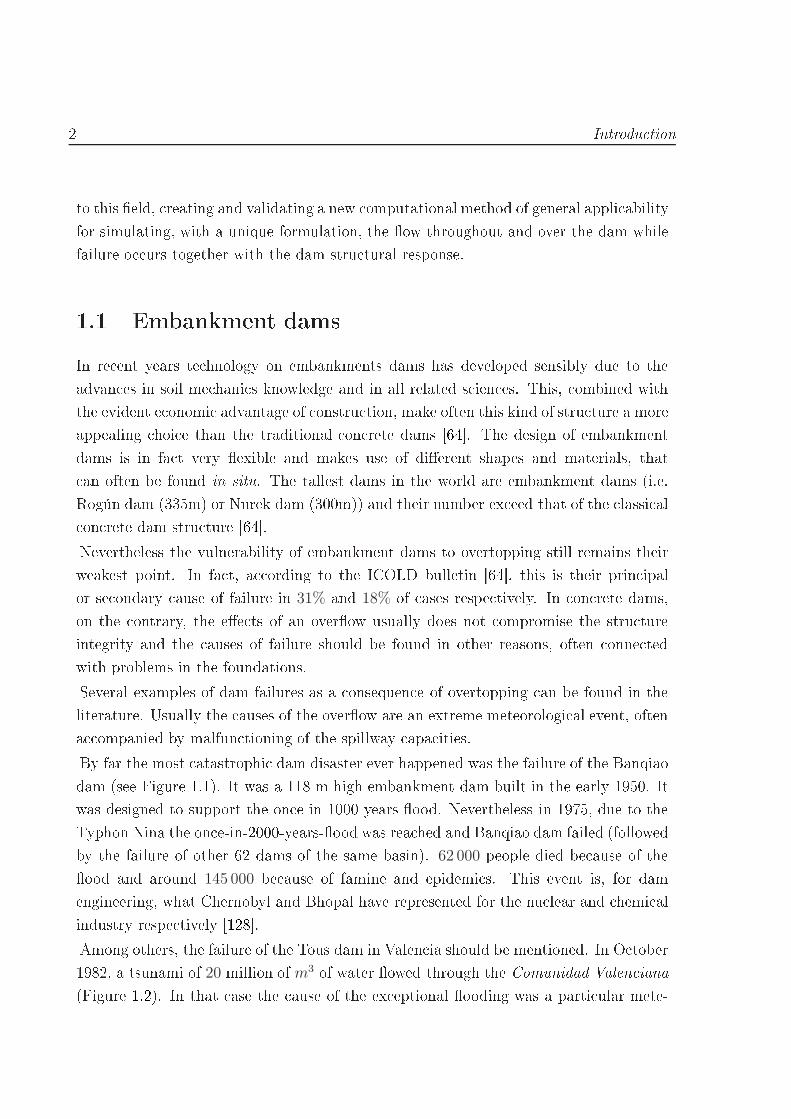
2 Introdu tionto this eld, reating and validating a new omputational method of general appli abilityfor simulating, with a unique formulation, the ow throughout and over the dam whilefailure o urs together with the dam stru tural response.1.1 Embankment damsIn re ent years te hnology on embankments dams has developed sensibly due to theadvan es in soil me hani s knowledge and in all related s ien es. This, ombined withthe evident e onomi advantage of onstru tion, make often this kind of stru ture a moreappealing hoi e than the traditional on rete dams [64. The design of embankmentdams is in fa t very exible and makes use of dierent shapes and materials, that an often be found in situ. The tallest dams in the world are embankment dams (i.e.Rogún dam (335m) or Nurek dam (300m)) and their number ex eed that of the lassi al on rete dam stru ture [64.Nevertheless the vulnerability of embankment dams to overtopping still remains theirweakest point. In fa t, a ording to the ICOLD bulletin [64, this is their prin ipalor se ondary ause of failure in 31% and 18% of ases respe tively. In on rete dams,on the ontrary, the ee ts of an overow usually does not ompromise the stru tureintegrity and the auses of failure should be found in other reasons, often onne tedwith problems in the foundations.Several examples of dam failures as a onsequen e of overtopping an be found in theliterature. Usually the auses of the overow are an extreme meteorologi al event, oftena ompanied by malfun tioning of the spillway apa ities.By far the most atastrophi dam disaster ever happened was the failure of the Banqiaodam (see Figure 1.1). It was a 118 m high embankment dam built in the early 1950. Itwas designed to support the on e-in-1000-years-ood. Nevertheless in 1975, due to theTyphon Nina the on e-in-2000-years-ood was rea hed and Banqiao dam failed (followedby the failure of other 62 dams of the same basin). 62 000 people died be ause of theood and around 145 000 be ause of famine and epidemi s. This event is, for damengineering, what Chernobyl and Bhopal have represented for the nu lear and hemi alindustry respe tively [128.Among others, the failure of the Tous dam in Valen ia should be mentioned. In O tober1982, a tsunami of 20 million of m3 of water owed through the Comunidad Valen iana(Figure 1.2). In that ase the ause of the ex eptional ooding was a parti ular mete-

Embankment dams 3

Figure 1.1: Image of Banqiao dam. Image taken from [1.

Figure 1.2: Image of Tous dam after the overtopping of O tober 19th, 1982.

4 Introdu tionorologi al ondition alled gota fria whi h onsists of a old high-altitude depressionsurrounded by warm air with high moisture ontent that leads to extremely heavy rainfall in the hinterland of the Mediterranean oast of Spain.These and many other similar histori al events demonstrate that when the water ex eedsthe rest of the dam, the onsequen es an be atastrophi . An ex eptional ooding ompromises seriously the stru ture, leading, in almost all ases, to its failure. Nev-ertheless the brea hing formation is a relatively slow pro ess. It is never an explosivesudden failure. Chanson in [30 for example, reported that in the ase of the Glashüttedam (Figure 1.3), the omplete failure of the stru ture o urs 4 hours later the begin-ning of the overtopping. In the ase of the Teton dam the reservoir was drained afterapproximately 12 hours.

Figure 1.3: Glashütte embankment dam (Germany). Image taken from [30.When the water overpasses the rest of the dam a seepage pro ess begins in the down-stream slope that leads to its progressive saturation. The rst brea h usually appearsat the toe of the dam, where the resistan e is lower. A ording to Toledo [122, 123, twoare the main me hanisms that ompromise the ro kll:• Mass sliding or loss of stability of a part of the downstream region due to the landslide. This is the predominant failure me hanism when the downstream slope isvery steep. The saturation of the ro kll leads to a redu tion of ee tive stressesthat, together with seepage, indu e the formation of a failure ir le that abruptly rumbles. This phenomenon usually ae ts the whole width of the dam as an beobserved in Figure 1.4(a).• Super ial dragging of ro kll parti les. When the downstream slope is at (1V :

The XPRES and E-DAMS proje ts 53H for instan e) this is the predominant failure me hanism. The water oming outfrom the toe of the dam drags away the super ial ro ks. It leads to the formationof hannels in the downstream slope (see for instan e Figure 1.4(b)).

(a) Mass sliding failure. (b) Super ial dragging failure.Figure 1.4: The images show two experiments arried out at the UPM laboratories. Onthe left an example of mass sliding failure (initial slope 1V : 1.5H) whereas on the rightthe failure is mainly due to super ial dragging of parti les (initial slope 1V : 3H).These two me hanisms usually a t in a ombined way depending on the failure pro essevolution [122.The lay ore represents an additional barrier before the omplete failure of the stru turewhen the prote tion given by the ro kll is no longer present (see Figure 1.5 for a typi al ross se tion of a ro kll dam). Its failure an be the onsequen e of surfa e erosion orof me hani al fra ture of the same under the pushing of the water retained upstream.CLAY CORE

ROCKFILL

FILTER

ROCKFILL

Downstream toeUpstream toeFigure 1.5: S hemati ross se tion of a ro kll dam.1.2 The XPRES and E-DAMS proje tsIn the last years the Spanish Ministry of S ien e and Innovation has been fundingthe XPRES [127 and E-DAMS [53 proje ts, a joint work between the Polyte hni

6 Introdu tionUniversity of Madrid (UPM), the Centre for Hydrographi al Studies of CEDEX and theInternational Centre for Numeri al Methods in Engineering (CIMNE).The prin ipal aim is the study of beginning and evolution of the brea h aused by anovertopping on ro kll prototype dams both from a physi al and numeri al point ofview.UPM and CEDEX team have a wide experien e on this topi and their eort hasbeen addressed to rea h a better hara terization of the failure in fun tion of a seriesof parameters. These are for examples, the downstream slope, the impervious systemadopted, the material used for the experiments and so on.Their extensive experimental ampaign onsists of more than 100 experiments. Furtherinformation an be found in Chapter 5 of the present work and for more details on thetopi , the onsultation of [21, 76 is re ommended.All the experiments have been performed in three umes of dierent dimensions shownin Figure 1.6.

(a) Small hannel.0.4m width, 0.6mheight, 12m long. (b) Medium hannel.1.0m width, 1.1mheight, 16m long. ( ) Large hannel. 2.48mwidth, 1.4m height, 13.7mlong.Figure 1.6: UPM and CEDEX experimental hannels used for XPRES and E-DAMSproje ts.The experimental data in terms of bottom pressure distribution and evolution of theseepage line, have been largely used in this work to validate the numeri al approa hof the .. ode during its development. Some examples of validation are presented inChapter 5.

Obje tives 71.3 Obje tivesThis work fa es the problem of the numeri al simulation of the overtopping and begin-ning of failure in a prototype ro kll dam.This leads to the development of two dierent numeri al tools:1. A uid ode to simulate a free surfa e ow in a variable porosity medium in orderto a urately predi t the hydrodynami for es a ting on the ro kll slope;2. A oupled uid-stru ture analysis ode to simulate the beginning of failure in aseof overtopping.The idea is to solve both problems (seepage and unset and evolution of failure), usinga ontinuous approa h and to integrate an Eulerian uid model with a Lagrangianstru tural one. This is done in order to minimize the omputational eort for theuid al ulation and to have a Lagrangian tool whi h an naturally following the largedeformation of the ro kll slope.Three are the main developments to be done in this work in order to a hieve its obje -tives:• A free surfa e uid model able to take into a ount the presen e of a porous media.It should work with any variable in oming dis harge ondition.• A stru tural model to simulate the behaviour of a ro kll slope in presen e (ornot) of variable hydrodynami for es.• A oupling tool to integrate the previously mentioned models and to simulatethe whole transitory phenomenon of failure of a ro kll slope due to ex eptionalooding.The assumption of a Newtonian in ompressible vis ous uid is taken for the ow ofwater. The solution system is a modied form of the traditional Navier-Stokes equations.The ee t of porosity is impli itly taken into a ount using the Dar y velo ity as avariable of the problem and adding the orresponding extra term in the momentumequations. This term takes into a ount the seepage for es.For the study of the uid behavior in a variable porosity medium an Eulerian approa hwith a xed mesh is hosen. A level set te hnique is used for the tra king of the evolutionof the free surfa e.

8 Introdu tionA Non-Newtonian onstitutive law is used to simulate the behaviour of a ro kll slope.A Bingham plasti with a variable yield threshold is proposed to a urately identifythe beginning of failure of the slope material, a ording to a Mohr Coulomb failure riteria. The Parti le Finite Element Method (PFEM) is the te hnique used for thestru tural analysis. Its Lagrangian approa h is a key feature to a urately follow thelarge distortion of the slope in ase of failure.The presen e of water should be taken into a ount in terms of variable hydrodynami for es. The problem is always fully drained sin e the pores an be onsidered inter on-ne ted a ording to experimental results.The oupling of the two models is done in an expli it staggered way by proje tinginformation between the Eulerian and the Lagrangian models. For that purpose a toolto proje t information between non-mat hing meshes is developed.The obje tives of this work an be onsidered fullled when the experiments on theprototype ro kll dams arried on by UPM and CEDEX an be reprodu ed.All the algorithms presented in this work have been implemented in Kratos [47, 48, aframework for developing nite element odes for multiphysi s problems.1.4 Layout of the do umentThe layout of the do ument is the following:Chapter 2. The physi al problem of seepage in ro kll is des ribed and the non linearform of the resistan e law governing the phenomena is hosen. A brief overviewof the state of the art is presented. The governing equations are derived and thenumeri al formulation is presented in detail. Two dierent Eulerian approa hesare des ribed, a traditional element-based approa h and an edge-based one. Inboth ases the level set te hnique is used to tra k the evolution of the free surfa e.Chapter 3. The behaviour of the ro kll material is treated as a non-Newtoniangranular uid. After an overview of traditional non-Newtonian materials, a regu-larized Bingham model is presented. This lassi al approa h is modied to takeinto a ount the variability of the yield stress in a granular non ohesive mate-rial. A Lagrangian kinemati al des ription is adopted and PFEM is used for thestru tural analysis.Chapter 4. The governing equations of the monolithi oupled problem are presented

Layout of the do ument 9and the balan e equation of the uid and stru ture models are derived The ou-pling is performed in a fully staggered way using a tool to manage the transferof informations between the two models. This is done using an algorithm thatallows the data mapping between non mat hing meshes, des ribed at the end ofthe hapter.Chapter 5. The ode is validated by reprodu ing experiments arried out by UPMand CEDEX using either 2D and 3D models. Dierent prototype dam models are onsidered in the examples.Chapter 6. The summary of the a hievements is des ribed and the main points of thefuture resear h work are outlined.Appendix A. The main features of Kratos Multiphysi s are briey presented.

Chapter 2The uid problemIn this hapter the numeri al algorithm developed for the simulation of the free surfa eow in presen e of a variable porosity medium is des ribed.First, a brief overview of the traditional studies of ux in porous media is performed inorder to hose a suitable resistan e law for the problem of interest. The balan e equationsare obtained and two solution strategies are adopted for their numeri al treatment. Anelement-based formulation and an edge-based approa h are studied and implemented.The hoi e of a xed mesh method leads to the need of tra king the evolution of thefree surfa e. The level set te hnique adopted for this purpose is des ribed in the lastpart of the hapter. The hapter nishes with a series of examples that aim to he kthe orre t behavior of the presented algorithms.2.1 Introdu tionThe lassi al approa hes of uid ow in porous media are not appli able for the analysisof the water motion within the ro kll of a dam. Traditionally water is onsidered inslow motion or as a stationary load [130. On the ontrary in the ase of an overtopping,the possibility to follow the rapid transition of the water level in the downstream slopeis a key point for the identi ation of the beginning of the failure me hanism.On the other hand, the typi al problem of evaluating the saturation level of the poresloses its importan e in the ase studied, due to the large dimension of the granularmaterial. Under these ir umstan es, in fa t, the pores an be onsidered always inter- onne ted and the problem fully drained [122.

12 The uid problemA ording to traditional studies of ow in porous media [117, 122, at a mi ro levelthe ux between the ro ks is assimilated to ow in pipes. This analogy is used for thederivation of the resistan e law used for the al ulation of the hydrauli gradient1 dueto seepage. The well known Dar y law is not appli able to the analyzed problem. Inthe following se tions it is explained how to obtain a suitable resistan e law to be usedin the balan e equations.It should be pointed out that a key point for the omplete simulation of the hydro-dynami ee t of an overtopping is the apability of the ode for simulating at on e,not only the seepage, but also the uid ow upstream, downstream and over the dam.For that purpose the balan e equations are derived onsidering the ow inside a generi porous material. The key point is represented by the fa t that they automati ally redu eto the lassi al Navier-Stokes equations when porosity is equal to one; that is when noporous medium is present. The resistan e law is inserted in the balan e equation as well.Its ontribution goes to zero out of the granular material. A similar approa h has beenused by Nithiarasu and oworkers [8890 to study the natural and for ed onve tiveux in a avity lled by a variable porosity medium.The easy denition of a ontrol domain and of spatial variables (like for instan e theporosity, dening the presen e of a granular material), indu es to hoose an Eulerianxed mesh approa h. Moreover this kinemati al framework is also more e ient allowingan easier parallelization of the ode.This hoi e leads to the need of hoosing a level set te hnique for tra king the evolutionof the free surfa e.Two dierent solution strategies are presented in the hapter, an element based and anedge based approa h. After a omparative analysis of both methodologies, the latter is hosen for being implemented in 3D and being oupled with the stru tural ode.2.1.1 Flow in ro kll materialThe ux in porous media is traditionally studied using the empiri al relation that Dar yobtained in 1856. Studying the ow of water through a sand-lled olumn he dis overedthat the pressure drop (i) and the velo ity of water inside a porous material (u) are1The hydrauli gradient is the measure of the variation of the hydrauli head for unit length [58.

Introdu tion 13linearly related. This observation leads to the formulation of the well known Dar y law,i =

µ

ku. (2.1)where µ is the water dynami vis osity and k is the permeability of the porous media[12.Relation 2.1 was derived studying the unidire tional ux in sand at low Reynolds num-bers. On the ontrary,in the ase of ux through ro kll material, the lo al uid ve-lo ities were observed not to be linearly related to the pressure drop. In fa t it wasexperimentally proved that over ertain average dimension of the parti les, equation 2.1is not anymore valid.Many authors have deeply studied this aspe t with essentially two obje tives:- Dis over the range of validity of Dar y's law (equation 2.1).- Dene an alternative resistan e law2 in ase equation 2.1 is not anymore valid.Remark 1. Velo ity u in equation 2.1 is by denition the Dar y velo ity, i.e. the uidvelo ity averaged over the total ontrol volume Ω (often alled ma ros opi velo ity orunit dis harge being the dis harge per unit volume), whereas the uid velo ity u isaveraged over the empty part of Ω ( alled ΩE). Their relation is stated by the Dupuit-For hheimer equation [87:

u = nu (2.2)where n is the porosity that, by denition 3 isn :=

ΩE

Ω. (2.3)See Figure 2.1 for a graphi al explanation.2Equation 2.1 and all the alternative non linear formulations that are presented in the next se tionsare ommonly alled resistan e laws be ause they measure the resistan e made by the porous matrixto the uid ow.3 Equation 2.3 is by denition the volumetri porosity nv whereas in Figure 2.1 a ross se tion ofthe ontrol volume is onsidered and a se tional porosity na := AE/A should be dened like the ratiobetween the area of pores and the total ross se tion area. Consequently, a lineal porosity an be alsodened as the ratio between the length of pores over the total length (nl := lE/l). Fortunately Bearsin [12 demonstrated that in a porous medium this distin tion is unne essary being

nv = na = nl.

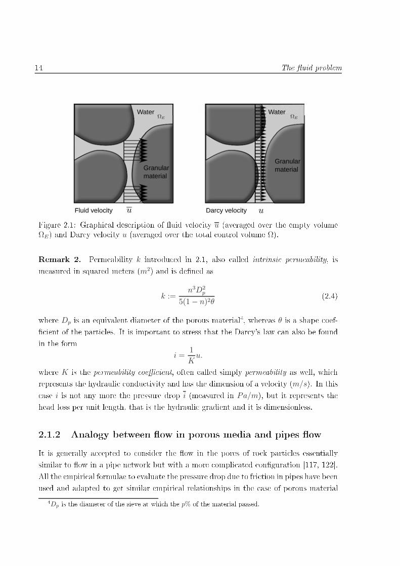
14 The uid problem

Darcy velocityFluid velocityFigure 2.1: Graphi al des ription of uid velo ity u (averaged over the empty volumeΩE) and Dar y velo ity u (averaged over the total ontrol volume Ω).Remark 2. Permeability k introdu ed in 2.1, also alled intrinsi permeability, ismeasured in squared meters (m2) and is dened as

k :=n3D2

p

5(1− n)2θ(2.4)where Dp is an equivalent diameter of the porous material4, whereas θ is a shape oef- ient of the parti les. It is important to stress that the Dar y's law an also be foundin the form

i =1

Ku.where K is the permeability oe ient, often alled simply permeability as well, whi hrepresents the hydrauli ondu tivity and has the dimension of a velo ity (m/s). In this ase i is not any more the pressure drop i (measured in Pa/m), but it represents thehead loss per unit length, that is the hydrauli gradient and it is dimensionless.2.1.2 Analogy between ow in porous media and pipes owIt is generally a epted to onsider the ow in the pores of ro k parti les essentiallysimilar to ow in a pipe network but with a more ompli ated onguration [117, 122.All the empiri al formulae to evaluate the pressure drop due to fri tion in pipes have beenused and adapted to get similar empiri al relationships in the ase of porous material4Dp is the diameter of the sieve at whi h the p% of the material passed.

Introdu tion 15[50, 79, 125.Some brief re all of ow in pipesThe Dar y-Weisba h formula is traditionally used for the evaluation of the hydrauli gradient i in pipes (only in a se ond time it was adapted to be used in open hannelows). It statesi =

fd4 rH

u2

2g; (2.5)where fd if the Dar y-Weisba h fri tion oe ient, rH is the hydrauli radius5 (in pipesof diameter D is rH = D/4), g is the gravity a eleration and u is the velo ity.In general fd is fun tion of the Reynolds number6(Re) and of the roughness of the pipe(e). It is demonstrated [58 that:- In laminar regime fd is a fun tion of Re only,

fd =64

Re.- In turbulent regime fd is onstant

fd = const.- In the transition regimefd = fd(Re, e).Above explanations imply that the hydrauli gradient, using equation 2.5, an be al- ulated as follow- For laminar regimei =

64µ

2gD2pρ

u. (2.6)- For turbulent regimei =

const

2g Dpu2. (2.7)5The hydrauli radius is dened as the ratio between the uid area and the wet perimeter.6The Reynolds number is the dimensionless oe ient that, being the ratio between inertia andvis ous for es, quanties the relative importan e of ea h one for a given ow [58. It is dened as ρu l

µwhere ρ is the uid density and l is a hara teristi length (in pipes it oin ide with the diameter).

16 The uid problemTherefore in ase of laminar regime, the relation between the hydrauli gradient andvelo ity is linear (like it is in Dar y's law), whereas in turbulent regime it be omesquadrati . Hen e, as a preliminary on lusion, the possibility to lassify whether theregime of the ux is turbulent or laminar seems to be very important to dene the rangeof validity of Dar y's law. Even though, as explained in the next se tions, this is notthe only aspe t to be taken into a ount.Denition of the range of validity of Dar y's lawMany dierent approa hes are present in literature on the appli ation of the Dar y-Weisba h relation to ow in porous media to dene the range of appli ation of Dar y'slaw. The deep analysis of ea h of them is not relevant for the aim of this work andthe onsultation of [79, 122 is re ommended for a more omprehensive understandingof the topi . Nevertheless some important aspe ts that led to the denition of dierentresistan e law are reported here to fully introdu e the problem.The main issue is related to the denition of the Reynolds number Re in a porousmaterial. In fa t the following aspe ts have to be taken into a ount:- Whether to take the velo ity of equation 2.5 equal to the Dar y velo ity (u) or tothe uid velo ity (u). This hoi e leads to a dierent denition of the ReynoldsnumberRe(u) =

u l

ν=

nu l

ν= nRe(u); (2.8)(equation 2.2 has been used).- How to dene the hara teristi length l in equation 2.8. Some authors prefer to hose an equivalent diameter Dp (often the hoi e is D10 or D50). In fa t it iseasier to measure the granular dimension than the dimension of the pores. Othersdene l ≈ rH arriving to express l as a fun tion of the permeability k.- Finally it is important to remember that equation 2.5 is one of the most popular,but not the only possible hoi e for the al ulation of the hydrauli gradient [50.Dierent hoi es lead to dierent values of Re. Nevertheless all authors agree that thebeginning of appearan e of turbulen e is for values of Re in the range 60 − 150 (not

2000 like in pipes).

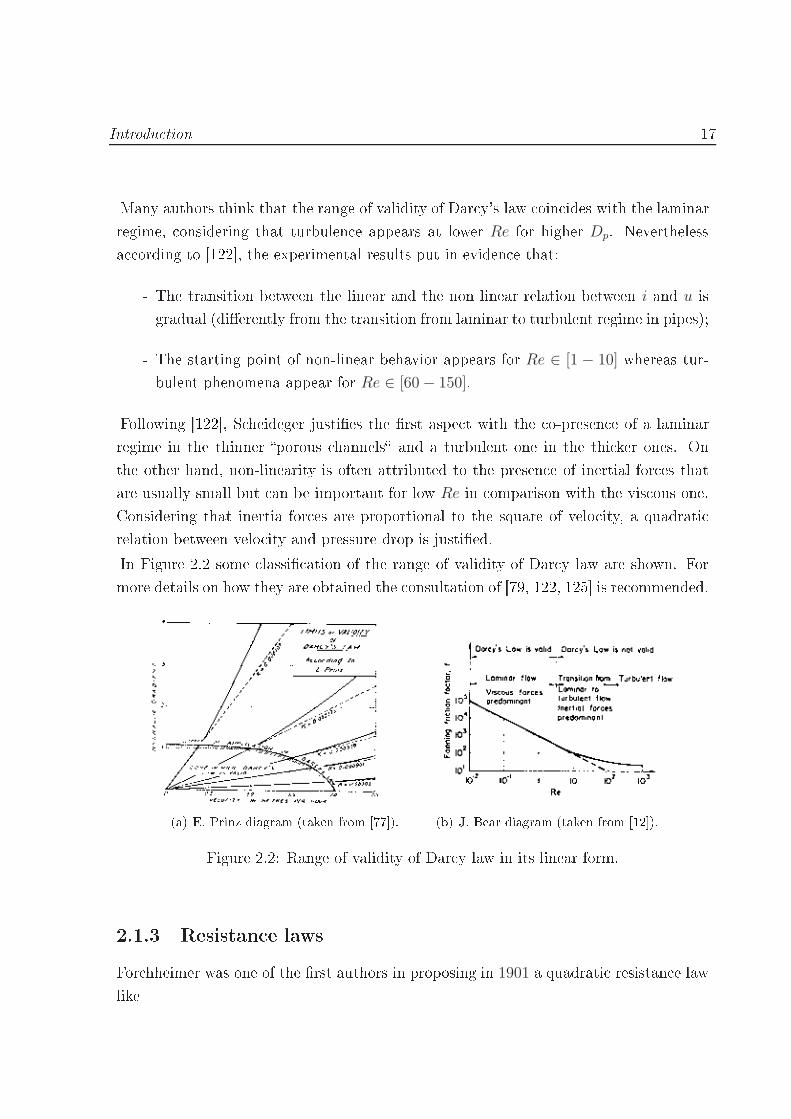
Introdu tion 17Many authors think that the range of validity of Dar y's law oin ides with the laminarregime, onsidering that turbulen e appears at lower Re for higher Dp. Neverthelessa ording to [122, the experimental results put in eviden e that:- The transition between the linear and the non linear relation between i and u isgradual (dierently from the transition from laminar to turbulent regime in pipes);- The starting point of non-linear behavior appears for Re ∈ [1 − 10] whereas tur-bulent phenomena appear for Re ∈ [60− 150].Following [122, S heideger justies the rst aspe t with the o-presen e of a laminarregime in the thinner porous hannels and a turbulent one in the thi ker ones. Onthe other hand, non-linearity is often attributed to the presen e of inertial for es thatare usually small but an be important for low Re in omparison with the vis ous one.Considering that inertia for es are proportional to the square of velo ity, a quadrati relation between velo ity and pressure drop is justied.In Figure 2.2 some lassi ation of the range of validity of Dar y law are shown. Formore details on how they are obtained the onsultation of [79, 122, 125 is re ommended.

(a) E. Prinz diagram (taken from [77). (b) J. Bear diagram (taken from [12).Figure 2.2: Range of validity of Dar y law in its linear form.2.1.3 Resistan e lawsFor hheimer was one of the rst authors in proposing in 1901 a quadrati resistan e lawlike

18 The uid problemi = αu+ βu2; (2.9)where onstants α and β depend only on the hara teristi s of ro kll material. Alter-natively Prony in 1804 and Jeager in 1956 proposed an exponential law like

i = γuη; (2.10)where γ and η depend on the ow ondition, the hara teristi s of the porous mediumand the uid.Both the quadrati and the power relationships are based on experimental results al-though some theoreti al basis have been provided for their justi ation [79. Nowadaysboth equations 2.9 and 2.10 are a epted and widely used. In re ent years almost alleorts have been addressed in determining the α and β or γ and η onstants.In fa t in some of the formulae the oe ients depend on physi al parameters of thero kll material only, su h as the size of the parti les, porosity and the parti le shape(following [122 this is the ase of Ergun (1952), Wilkins(1956), M Corquodale (1978),Stephenson(1979), Martins (1990) and Gent (1991)). In other ases, the oe ients de-pend on the experimental value of the hydrauli ondu tivity. Sin e building prototypesfor estimating these parameters an be very expensive, it is often easier and heaper to hoose one of the rst group of formulae.A omprehensive overview of the dierent models an be found in [79, 122, 125.Sele tion of the seepage model: Ergun's orrelationIn the previous paragraphs an overview of the state of the art of seepage models hasbeen presented. In order to hoose the suitable non-linear resistan e law to be used inthis work, some additional remarks should be done.- The obje tive of the model is to develop a tool to simulate the free surfa e owthrough the ro kll and outside of the same, so an essential requirement for theresistan e law is that it should automati ally go to zero when n = 1.- The quadrati form of the resistan e laws is easier to implement than the expo-nential one;Colle ting the previous onsiderations, a quadrati form of the non-linear resistan elaw is adopted and the Ergun's denition of the onstant oe ients is hosen [57.

Continuous form 19Therefore, the pressure drop isi = E1u+ E2u

2; (2.11)Following Ergun theory and alling Dp the average diameter of the granular material(Dp ≡ D50), E1 and E2 oe ients are dened likeE1 = 150 · (1− n)2

n3· µ

D2p

; (2.12)andE2 = 1.75 · (1− n)

n3· ρ

Dp; (2.13)Dening the permeability shape oe ient θ = 30 of equation 2.4, the permeability k an be al ulated as a fun tion of n and Dp

k =n3D2

p

150(1− n)2. (2.14)The nal form of the resistan e law hosen in this work is then:

i =µ

ku+

1.75√150

ρ√kn3/2

u2. (2.15)It is interesting to observe that the linear part of equation 2.15 is equivalent to theDar y's law2.2 Continuous formOn e the resistan e law has been hosen, the balan e of linear momentum and the ontinuity equation for an in ompressible uid an be derived. The prin ipal obje tiveof the present approa h is to dene a unique set of balan e equations governing both thefree surfa e ow and the seepage problem. In other words the governing equations haveto be able to reprodu e the free surfa e ow in a variable porosity medium ( onsideringthe open air as a porous medium with porosity n = 1).An approa h similar to the one presented in the following se tions, an be found in hapter 5 of the 5th edition of [132. This methodology is largely used for the treatmentof heat transfer in a uid saturated porous media [8, 88, 89, 124.

20 The uid problem2.2.1 Variables of the problemThe unknowns of the problem are:- u, uid Dar y velo ity (see equation 2.2 for its denition).- p, uid pressure;Other parameters are:- ρ is the uid density. In the present work water is treated as an in ompressibleuid with onstant density over the whole uid domain, regardless of the presen eof a porous medium.- µ is the uid dynami vis osity.- n is the porosity (see equation 2.3 for its denition). In the most general ase itis a fun tion of spa e and time:n = n(x, t); (2.16)In the present work, a ording to experimental analysis, the variation of porosityin time, within the uid solver, an be negle ted, onsidering only its variationin spa e. Nevertheless it should be remarked that porosity does hange in timea ording to the stru tural deformation of the porous material, whi h will beexplained in hapter 3 and has been onsidered in the oupled problem des ribedin hapter 5.Therefore, as a uid variable, n is only fun tion of the spatial oordinatesn = n(x); (2.17)The uid is onsidered here as a ontinuum and the presen e of a porous matrix isimpli itly taken into a ount via the porosity n as will be explained in se 2.2.3.2.2.2 Constitutive law. Water as a Newtonian in ompressibleuidThe water is treated as a Newtonian in ompressible uid. In general a uid at rest doesnot present shear stresses and the Cau hy stress tensor takes the form σ = −pI. The

Continuous form 21tangential stresses are non zero in a uid in motion and the stress tensor be omesσ := −pI+ τ (2.18)where τ is the deviatori part. The latter is linearly related to the strain rate tensorthrough vis osity whi h is assumed to be onstant.Therefore the stress tensor for a Newtonian uid is

σ := −pI+ 2µ∇su; (2.19)where µ is the dynami vis osity and(∇su)kl :=

1

2

(∂uk

∂xl+

∂ul

∂xk

)

; (2.20)is the symmetri part of the velo ity gradient [51, 132. It should be observed thatequation 2.19 does not take into a ount the possible presen e of a porous medium. Amore general form of the same will be derived in the next se tions in order to have arelation that holds both for the ase of free uid and of ow in ro kll material.2.2.3 Modied form of the Navier-Stokes equationsIn order to take into a ount the ow in a variable porosity medium, some modi ationsshould be introdu ed in the traditional form of the Navier-Stokes equations. The mod-ied system of solution equations is derived here imposing ontinuity and onservationof linear momentum within a xed ontrol volume.In the following se tions a balan e on a nite volume is rst arried out and broughtlater to the innitesimal form.Remark 3. It is important to stress that it is always used a ontinuous approa h totreat the uid in the whole domain regardless of it is inside or not the porous media.Continuity equationLet us onsider a 2D square nite ontrol volume dxdy as the one plotted in Figure2.3, and let's dene dxdy = n dxdy as the empty part of it, that is the portion of thisvolume that an be o upied by the uid (see the denition of porosity at equation 2.3).

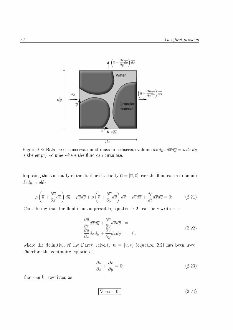
22 The uid problem

Figure 2.3: Balan e of onservation of mass in a dis rete volume dx dy. dxdy = n dx dyis the empty volume where the uid an ir ulate.Imposing the ontinuity of the uid eld velo ity u = [u, v] over the uid ontrol domaindxdy, yields

ρ

(

u+∂u

∂xdx

)

dy − ρudy + ρ

(

v +∂v

∂ydy

)

dx− ρvdx+dρ

dtdxdy = 0; (2.21)Considering that the uid is in ompressible, equation 2.21 an be rewritten as

∂u

∂xdxdy +

∂v

∂ydxdy =

∂u

∂xdxdy +

∂v

∂ydxdy = 0.

(2.22)where the denition of the Dar y velo ity u = [u, v] (equation 2.2) has been used.Therefore the ontinuity equation is∂u

∂x+

∂v

∂y= 0; (2.23)that an be rewritten as

∇ · u = 0; (2.24)

Continuous form 23Momentum equationThe balan e of linear momentum in the i− th dire tion isρdui

dtdxdy − ∂σij

∂xjdxdy − ρf ext

i dxdy = 0; (2.25)where f ext are the volumetri for es and the sum over j spatial index is supposed.Observing Figure 2.4 and remembering that the onstitutive equation 2.19 is[

σx τxy

τxy σy

]

= −[

p 0

0 p

]

+ 2µ

[

∂u/∂x 1/2 (∂u/∂y + ∂v/∂x)

1/2 (∂u/∂y + ∂v/∂x) ∂v/∂y

](2.26)

Figure 2.4: Balan e of onservation of linear momentum in a dis rete volume dx dy.dxdy = n dx dy is the empty volume where the uid an ir ulate.the balan e equation in x-dire tion be omes

24 The uid problemρ∂u

∂tdxdy + ρu

∂u

∂xdxdy ++ρv

∂u

∂ydxdy

−∂σx

∂xdxdy +

∂τxy∂y

dxdy − ρbxdxdy + Dxdxdy = 0;(2.27)where the Dx represents the x omponent of the hydrauli gradient due to seepage, e.g.the resistan e law dis ussed in Se tion 2.1.3 (i.e. equation 2.15). Its matri ial form willbe detailed at the end of this se tion. In equation 2.27 the denition of material timederivative has been impli itly taken into a ount (ρdui

dt= ρ

∂u

∂t+ ρu

∂u

∂x++ρv

∂u

∂y

).Substituting dxdy = n dxdy into equation 2.27 and inserting the denition of Dar yvelo ity givesρ∂u

∂t+ ρu

∂u

∂x+ ρv

∂u

∂y+ n

∂p

∂x

−2µ∂2u

∂x2− µ

(∂2u

∂x∂y+

∂2v

∂x2

)

n− ρbxn+ nDx = 0;(2.28)This expression holds for any innitesimal domain dxdy.Finally, alling Dy = nDy, and using the same pro edure in the other spatial dimensionleads to analogous results. In summary the equation of balan e of linear momentum iswritten as

ρ∂tu+ ρu · ∇u+ n∇p− 2∇ · µ∇su− ρbn +D = 0; (2.29)where ∂tu =∂u

∂t. In equation 2.29 D is the matri ial form of the resistan e law 2.15or, what is the same, the Dar y term. It represents the dissipative ee ts due to theintera tion between the solid and the uid part. Details of this term an be found inSe tion 2.1.3. The matri ial form of the non-linear Dar y's law 2.15 is

D =nµ

ku+

1.75√150

ρn√k

|u|n3/2

u. (2.30)Remark 4. Let us dene the Ergun oe ients E1 and E2 per unit density as

E1 = 150 · (1− n)2

n2· µ

D2pρ

; (2.31)

Weak form 25andE2 = 1.75 · (1− n)

n2· 1

Dp. (2.32)These expressions will be useful in the next hapter espe ially during the explanationof the stabilization te hniques.Remark 5. A more general form of the onstitutive equation of water an be nowformulated as

σ := −npI + 2µ∇su. (2.33)This equation automati ally redu es to equation 2.19 if the porosity is equal to one (i.e.the free surfa e ow problem is onsidered).2.3 Weak formEquation 2.24 and 2.29 represent the modied form of the Navier-Stokes problem. Theytake into a ount the presen e of a porous medium and redu e to the lassi al NavierStokes equations when the porosity is n = 1 (free uid ow). The equations to be solvedare thereforeρ∂tu+ ρu · ∇u+ n∇p− 2∇ · µ∇su

−ρbn + E1u+ E2|u|u = 0 in Ω, t ∈ (0, T );

∇ · u = 0 in Ω, t ∈ (0, T ).

(2.34)where Ω ⊂ Rd (where d is the spa e dimension) is the uid domain in a time interval

(0, T ).The boundary and initial ondition of the previous problem are:u(x, 0) = u0(x) in Ω;

u(x, t) = g(x, t) on ∂ΩD , t ∈ (0, T );

n · σ(x, t) = t(x, t) on ∂ΩN , t ∈ (0, T );

(2.35)where σ is dened by equation 2.33 and ΩD and ΩN are the Diri hlet and Neumannboundary respe tively.Remark 6. Note that n indi ates the outer unit normal ve tor whereas n is dened inequation 2.3 and indi ates the porosity.

26 The uid problemThe weak form of equations 2.34 is derived next using a Galerkin formulation. A mixednite element method is obtained, that is the approximation of both the velo ity ompo-nents and the pressure (and their respe tive weighted fun tions) need to be introdu ed.The weak form of equation 2.34 is∫

Ω

wρ∂tudΩ +

∫

Ω

wρu · ∇udΩ+

∫

Ω

wn∇pdΩ

−∫

Ω

w∇ · 2µ∇sudΩ+

∫

Ω

w(E1u+ E2|u|u)dΩ−∫

Ω

wρnbdΩ = 0 ∀w ∈ V;∫

Ω

q∇ · u = 0 ∀q ∈ Q;

(2.36)where, for a xed t ∈ (0, T ), u is assumed to belong to the velo ity spa e V ∈ [H1(Ω)]dof ve tor fun tions whose omponents and their rst derivatives are square-integrable,and p belongs to the pressure spa e Q ∈ L2 of square-integrable fun tions. w and qare velo ity and pressure weighting fun tions belonging to the velo ity and the pressurespa es respe tively. Integrating by parts the pressure and onve tive terms, allingΓ = ∂Ω gives

∫

Ω

wn∇pdΩ = −∫

Ω

np∇ ·wdΩ+

∫

∂Ω

w · npndΓ;∫

Ω

w∇ · 2µ∇sudΩ = −2∫

Ω

∇w : µ∇sudΩ+

∫

∂Ω

w · (2µn · ∇su)dΓ;(2.37)where n is the outer normal ve tor (see remark 6). Substituting relations 2.37 intoequations 2.36 and onsidering the Neumann boundary ondition, the system to besolved be omes

∫

Ω

wρ∂tudΩ +

∫

Ω

wρu · ∇udΩ−∫

Ω

np∇ ·wdΩ

+2

∫

Ω

∇w : µ∇sudΩ +

∫

Ω

w(E1u+ E2|u|u)dΩ

−∫

Ω

wρnbdΩ−∫

∂ΩN

w · tdΓ = 0 ∀w ∈ V;∫

Ω

q∇ · udΩ = 0 ∀q ∈ Q;

(2.38)Let Vh be a nite element spa e to approximate V, and Qh a nite element approxima-

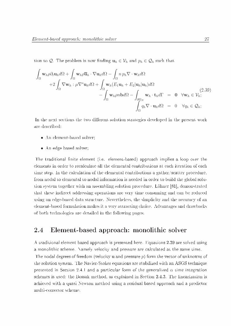
Element-based approa h: monolithi solver 27tion to Q. The problem is now nding uh ∈ Vh and ph ∈ Qh su h that∫

Ω

whρ∂tuhdΩ+

∫

Ω

whρuh · ∇uhdΩ−∫

Ω

n ph∇ ·whdΩ

+2

∫

Ω

∇wh : µ∇suhdΩ+

∫

Ω

wh(E1uh + E2|uh|uh)dΩ

−∫

Ω

whρnbdΩ−∫

∂ΩN

wh · thdΓ = 0 ∀wh ∈ Vh;∫

Ω

qh∇ · uhdΩ = 0 ∀qh ∈ Qh;

(2.39)In the next se tions the two dierent solution strategies developed in the present workare des ribed:• An element-based solver;• An edge-based solver;The traditional nite element (i.e. element-based) approa h implies a loop over theelements in order to re al ulate all the elemental ontributions at ea h iteration of ea htime step. In the al ulation of the elemental ontributions a gather/s atter pro edure,from nodal to elemental to nodal information is needed in order to build the global solu-tion system together with an assembling solution pro edure. Löhner [81, demonstratedthat these indire t addressing operations are very time onsuming and an be redu edusing an edge-based data stru ture. Nevertheless, the simpli ity and the a ura y of anelement-based formulation makes it a very attra ting hoi e. Advantages and drawba ksof both te hnologies are detailed in the following pages.2.4 Element-based approa h: monolithi solverA traditional element based approa h is presented here. Equations 2.39 are solved usinga monolithi s heme. Namely velo ity and pressure are al ulated at the same time.The nodal degrees of freedom (velo ity u and pressure p) form the ve tor of unknowns ofthe solution system. The Navier-Stokes equations are stabilized with an ASGS te hniquepresented in Se tion 2.4.1 and a parti ular form of the generalized α time integrations hemes is used: the Bossak method, as explained in Se tion 2.4.3. The linearization isa hieved with a quasi Newton method using a residual based approa h and a predi tormulti- orre tor s heme.

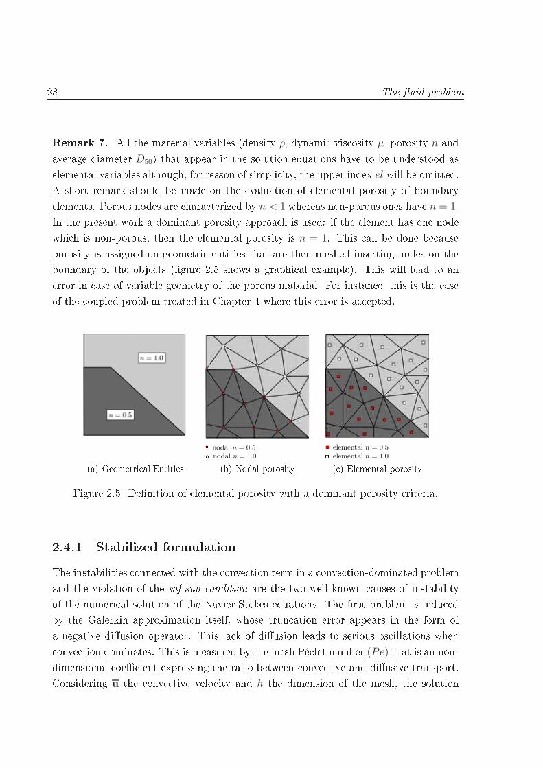
28 The uid problemRemark 7. All the material variables (density ρ, dynami vis osity µ, porosity n andaverage diameter D50) that appear in the solution equations have to be understood aselemental variables although, for reason of simpli ity, the upper index el will be omitted.A short remark should be made on the evaluation of elemental porosity of boundaryelements. Porous nodes are hara terized by n < 1 whereas non-porous ones have n = 1.In the present work a dominant porosity approa h is used: if the element has one nodewhi h is non-porous, then the elemental porosity is n = 1. This an be done be auseporosity is assigned on geometri entities that are then meshed inserting nodes on theboundary of the obje ts (gure 2.5 shows a graphi al example). This will lead to anerror in ase of variable geometry of the porous material. For instan e, this is the aseof the oupled problem treated in Chapter 4 where this error is a epted.

(a) Geometri al Entities (b) Nodal porosity ( ) Elemental porosityFigure 2.5: Denition of elemental porosity with a dominant porosity riteria.2.4.1 Stabilized formulationThe instabilities onne ted with the onve tion term in a onve tion-dominated problemand the violation of the inf-sup ondition are the two well known auses of instabilityof the numeri al solution of the Navier-Stokes equations. The rst problem is indu edby the Galerkin approximation itself, whose trun ation error appears in the form ofa negative diusion operator. This la k of diusion leads to serious os illations when onve tion dominates. This is measured by the mesh Pé let number (Pe) that is an non-dimensional oe ient expressing the ratio between onve tive and diusive transport.Considering u the onve tive velo ity and h the dimension of the mesh, the solution

Element-based approa h: monolithi solver 29presents a la k of diusion ifPe :=

uh

2µ≥ 1;i.e. when onve tion dominates over diusion [51.The se ond reason of instability is onne ted with the hoi e of the nite element spa efor pressure and velo ity.In order to better understand the origin of this kind of instability it is onvenient tore all the lassi al stationary Stokes problem

−ν∆u +∇p = b;

∇ · u = 0;(2.40)that, in matrix form, be omes

[

K G

D 0

] [

u

p

]

=

[

F

0

] (2.41)where K = −νL ← −ν∆ is the vis ous operator (being L the Lapla ian), G is thedis rete gradient operator, D is the divergen e operator (D = GT ) , u is the ve tor ofnodal velo ities, p is the ve tor of nodal pressures and F is the external for e ve tor.The zero matrix on the lower diagonal position of the system matrix, derived from theimposition of the in ompressibility onstrain, leads to some restri tions in the numeri alsolvability of the problem. It an be shown that the solution of system 2.41 exists and itis unique (i.e. the global matrix 2.41 is non-singular) if the kernel7 of matrix G is zero.In fa t from the rst equation it is possible to get u = K−1(F −Gp) that substitutedin the se ond equation leads to(DK−1G)p = (DK−1F);where DK−1G is symmetri , being K symmetri , but it is positive denite only if

ker G = 0. In the latter ase the pressure matrix is non singular and the value of p anbe al ulated and substituted in order to evaluate u [51.Ladyzhenskaya - Babuska - Brezzi demonstrated that both the ontinuous and thedis rete spa e of velo ity and pressure (see Se tion 2.3 for their denition) annot bearbitrarily hosen but they have to satisfy the so alled inf-sup (or LBB from the initials7 The kernel of a matrix A is dened as kerA := q | q ∈ Rd and Aq = 0.

30 The uid problemof the authors) ondition. It states that a stable nite element solution uh,ph to theStokes problem exists if it is ensured that∀ ph ∈ Qh ∃ uh ∈ Vh su h that β||ph|| ||uh||H1 ≤ b(ph,uh); (2.42)or equivalently

infph∈Qh

supuh∈Vh

b(ph,uh)

||ph|| ||uh||H1

≥ β; (2.43)where b(, ) is the bilinear form b(ph,uh) = −∫

Ωph∇ · uhdΩ and || || is the L2 normwhereas || ||H1 is the H1 norm [9, 16.There are several pairs of pressure velo ity interpolations that allow the satisfa tionof 2.43 like for instan e the Q1/P0 element ( ontinuous bilinear velo ity, dis ontinuous onstant pressure), or the Q2/P1 multiquadrati velo ity, pie ewise linear pressure or,among the ontinuous pressure interpolations, the so alled mini-element (P1 + /P1)for example, with a linear velo ity enri hed with an internal bubble and linear pressure.More details an be found in [10, 42, 51, 106.Unfortunately the simplest element, the P1/P1 (pie ewise linear velo ity and pressure),whi h is used in the present work for pra ti al reasons, does not satisfy the inf-sup ondition and a stabilization te hnique is ne essary to xed both sort of instability.A wide range of stabilization te hniques an be found in literature. One of the rst ideasto over ome numeri al os illations on onve tion dominated problems, was to introdu ediusion on the dire tion of the stream lines. This led to the lassi al and extensivelyused streamline-upwind/Petrov-Galerkin (SUPG) method by Brooks and Hughes [17.A generalization of SUPG for Stokes ows was proposed by Tezduyar [120, 121: thepressure-stabilizing/Petrov-Galerkin (PSPG). In this ase the stabilization term varieswith the Reynolds number. In the zero Reynolds number limit, the PSPG stabilizationterm redu es to the SUPG one. Another, more general, stabilization approa h wasproposed by Hughes [63 (the Galerkin least-squares or GLS). He found out a wayto use an equal order interpolation for velo ity and pressure for the Stokes problemfor in ompressible uids just adding the pressure gradient in the stabilizing terms in aSUPG-like strategy. The GLS method for time dependent problems uses both spa e andtime nite elements dis retization leading to a spa e-time nite element formulation ofthe problem.So far all the stabilization te hniques presented require the addition of some arti ialdiusion term. As an alternative Oñate derived the stabilization terms using a Finite

Element-based approa h: monolithi solver 31 al ulus (FIC) approa h based on imposing the balan e equations over a nite domain[92, 93, 97, 101. This approa h allows to reinterpret the stabilization terms as anintrinsi and natural ontribution to the original dierential equations, instead of a orre tion term introdu ed at dis rete level. With this natural stabilization approa hmany of the already existing stabilization te hniques an be reinterpreted in a morephysi al manner.A popular family of stabilization methods is derived by the so alled subgrid s ale (SGS)approa h, introdu ed by Hughes in [62. His novel idea is to split the unknowns (u) intoa part that an be represented by the nite element mesh (uh) and another part thata ounts for the unresolvable s ale (u), that is for the variation of the unknown that annot be aptured by the nite element mesh. This orresponds to a splitting of thespa e V into the spa e of the nite elements (Vh) and the subgrid spa e (V) asV = Vh ⊕ V ; (2.44)Among the dierent SGS methods, two are the hosen te hniques used in this work:- The Algebrai Sub-Grid S ale stabilization (ASGS) that has been implemented inthe element based formulation;- The Orthogonal Subgrid S ale (OSS) te hnique that has been employed to stabilizethe edge-based equations (see Se tion 2.5.1).The main dieren e between these two te hniques is that in ASGS the whole residualis used to approximate the sub-s ales whereas in OSS only its orthogonal proje tion isused.Typi ally, stabilized methods add to the left hand side of the dis rete residual of theproblem (i.e. the dis retized weak form), a term of the form

r(uh,wh) =∑

el

∫

Ωel

Pel(wh)T τ elRel(uh)dΩ; (2.45)where the so alled intrinsi time, τ el is an algorithmi parameter with dimension oftime, Pel(wh) is a ertain operator applied to the test fun tion (it will be dened lateron) and Rel(uh) is the residual of the dierential equation to be solved. The upper index

el in equation 2.45 indi ates that the ontribution is element-wise and will be omittedlater on for the sake of simpli ity.

32 The uid problemLet us introdu e the stabilized form of equation 2.39 using an ASGS te hnique.Referring to equation 2.45 Table 2.1 an be obtained. α ∈ [0, 1] is an input parameterto ontrol the inuen e of dynami ontribution, h is the element length8. The upper-indexes m and c refer to the momentum and the ontinuity equation respe tivelyMomentum equation

Pm(wh) uh · ∇wh +∇qh

τ1

(α

∆t+

4ν

h2+

2|uh|h

+ E1 + E2|uh|)−1

Rm(uh) ∂tuh + uh · ∇uh − ν∆uh + n∇ph + E1uh + E2|uh|uh − nbContinuity equationPc(wh) ∇ ·wh

τ2µ

ρ+

h|uh|2

Rc(uh) ∇ · uhTable 2.1: Stabilizing elemental terms in the ASGS method.Therefore the stabilized problem be omes:∫

Ω

whρ∂tuhdΩ +

∫

Ω

whρuh · ∇uhdΩ−∫

Ω

n ph∇ ·whdΩ

+2

∫

Ω

∇wh : µ∇uhdΩ +

∫

Ω

wh(E1uh + E2|uh|uh)dΩ

−∫

Ω

whρnbdΩ−∫

∂ΩN

whthdΓ +∑

el

∫

Ωel

τ1Pm · RmdΩ = 0 ∀wh ∈ Vh;∫

Ω

qh∇ · uhdΩ+∑

el

∫

Ωel

τ2Pc · RcdΩ = 0 ∀qh ∈ Qh;

(2.46)8The element length is dened as the edge of a regular triangle in 2D (or of a regular tetrahedronin 3D), ins ribed in the ir umferen e (sphere in 3D) that ir ums ribes the element itself.

Element-based approa h: monolithi solver 332.4.2 Dis retization pro edureCalling u and p the ve tor of nodal velo ities and pressures respe tively, system 2.46 inits matri ial form is expressed as[

M 0

0 0

]

·[

u

p

]

+

[

K G

D 0

]

·[

u

p

]

=

[

F

0

] (2.47)where the orresponden e between the blo k matri es of 2.47 and the ontinuum formof the solution equation 2.39 an be seen in Table 2.2. Every blo k matrix is obtained, asusual, from the assembling of elemental ontributions. Ea h node has as many degreesof freedom as the spa e dimension (nsd) plus 1. That is the upper left elemental blo kmatrix (K) has dimensions nsd × nsd and G is a nsd × 1 matrix ( onsequently D is a1×nsd). Therefore the global stiness matrix is a square matrix of npts · (nsd+1)×npts ·(nsd + 1) (where npts is the number of nodes). The nonlinear terms are treated usingthe Pi ard method and they are evaluated at the element Gauss points at the previousiterations.The matrix form of the stabilized system of equation 2.46 an be written as:[

M+ SMwu 0

0 0

]

·[

u

p

]

+

[

K+ Swu + Sc G+ Swp

D+ Squ Spq

]

·[

u

p

]

=

[

F+ Sfw

Sfq

] (2.48)where all the stabilization matri es are inserted. Their detailed meaning an be foundin Table 2.3 where Swv = SCwv + Sµ

wv + SDwv and Squ = SC

qu + Sµqu + SD

qu.Equation 2.48 an be written in ompa t form asMv + fint(v(t), t) = fext(t); (2.49)where vT = [u, p] and vT = [u, p] are the ve tor of unknowns and their time derivativesrespe tively.

34 The uid problem

Matri ial term Continuum termMu

∑

el

∫

Ωel

whρ∂tuhdΩ

KCu∑

el

∫

Ωel

whρuh · ∇uhdΩ

Ku Kµu −2∑

el

∫

Ωel

wh∇wh : µ∇uhdΩ

KDu∑

el

∫

Ωel

wh(E1uh + E2|uh|uh)dΩ

Gp −∑

el

∫

Ωel

n ph∇ ·whdΩ

Du∑

el

∫

Ωel

qh∇ · uhdΩ

F∑

el

∫

Ωel

whρnbdΩTable 2.2: Matri es and ve tors of system 2.48 without stabilization terms.

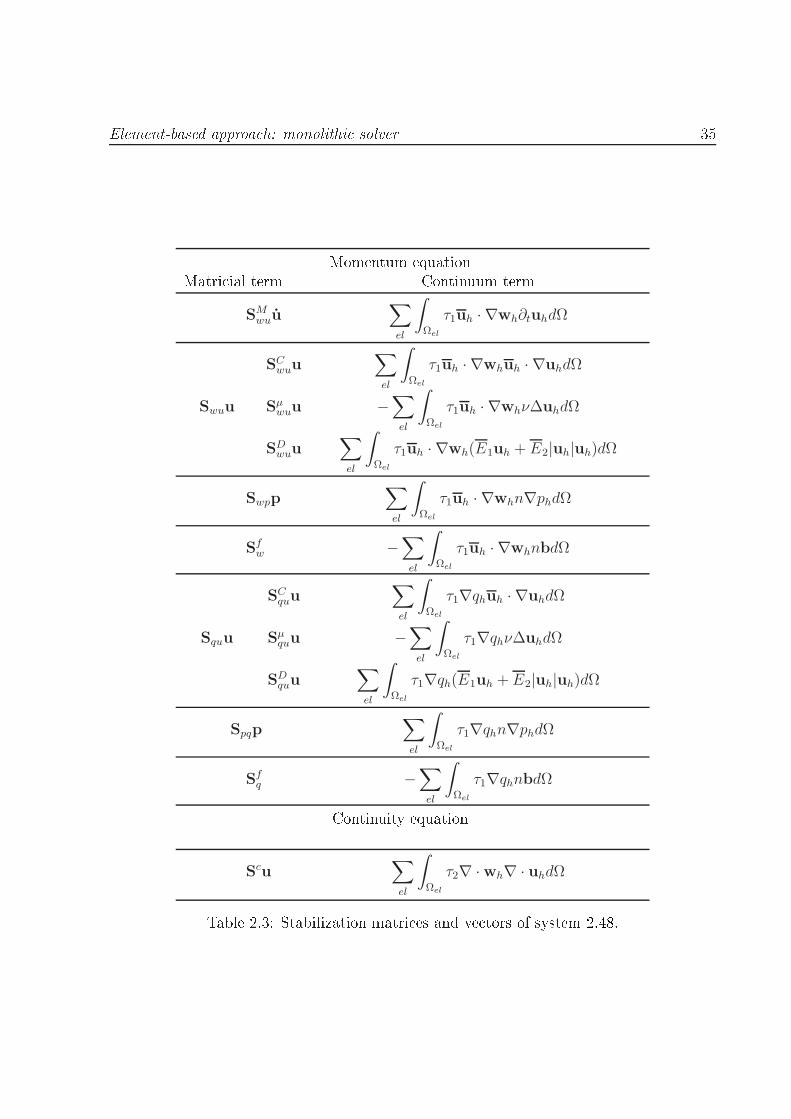
Element-based approa h: monolithi solver 35Momentum equationMatri ial term Continuum term

SMwuu

∑

el

∫

Ωel

τ1uh · ∇wh∂tuhdΩ

SCwuu

∑

el

∫

Ωel

τ1uh · ∇whuh · ∇uhdΩ

Swuu Sµwuu −

∑

el

∫

Ωel

τ1uh · ∇whν∆uhdΩ

SDwuu

∑

el

∫

Ωel

τ1uh · ∇wh(E1uh + E2|uh|uh)dΩ

Swpp∑

el

∫

Ωel

τ1uh · ∇whn∇phdΩ

Sfw −

∑

el

∫

Ωel

τ1uh · ∇whnbdΩ

SCquu

∑

el

∫

Ωel

τ1∇qhuh · ∇uhdΩ

Squu Sµquu −

∑

el

∫

Ωel

τ1∇qhν∆uhdΩ

SDquu

∑

el

∫

Ωel

τ1∇qh(E1uh + E2|uh|uh)dΩ

Spqp∑

el

∫

Ωel

τ1∇qhn∇phdΩ

Sfq −

∑

el

∫

Ωel

τ1∇qhnbdΩContinuity equationScu

∑

el

∫

Ωel

τ2∇ ·wh∇ · uhdΩTable 2.3: Stabilization matri es and ve tors of system 2.48.

36 The uid problem2.4.3 Bossak time integration s hemeThe Navier-Stokes equations are solved in time using a Bossak s heme. First of all, letus re all the Newmark s heme from whi h it takes its origin. This is one of the mostpopular time integration pro edures in stru tural dynami s and it is used with su essin the linear regime. Its use in non-linear problems is possible, however in presen e oflarge geometri non-linearities it is known to lead to unstable results unless the time stepis severely redu ed. This drawba k derives form the fa t that, in the stability of linearproblems, the balan e of energy equation implies an upper bound to the solutions. Onthe ontrary, in a non linear regime this is not automati ally veried when a linearizationis performed. A stable algorithm an diverge in problems in whi h energy an grow upunlimitedly. It is therefore ne essary to introdu e some parameters in the time s hemeable to lead to energy dissipation in high frequen y modes [61, 118.The momentum equation in stru tural problems is written in the general form asMx +Cx +Kx = f ext; (2.50)where x is the ve tor of displa ements and M, C, K are the stabilized mass, dampingand stiness matri es respe tively. The overbar is used to distinguish the stabilizedoperators from those presented in equation 2.47.Let's all vT = [u, p] and vT = [u, p] the ve tor of unknowns and their time derivativesrespe tively. Equation 2.50, rewritten in terms of v and its derivative, represents the ompa t form of equations 2.48. It is

Mv + fint(v(t), t) = fext(t); (2.51)where M is the mass matrix. fint takes into a ount of all the terms that dependson velo ity and pressure (the internal for es) and fext is the ve tor of external for es,in luding all the ontributions independent from the unknowns. Let's remark thatequation 2.51 is an alternative way of writing equation 2.48.Following the Newmark formulation v and x an be obtained at time step n+ 1 asvn+1 = vn + (1− δ)∆t vn + δ∆tvn+1; (2.52a)xn+1 = xn +∆tvn +

(1

2− β

)

∆t2vn + β∆t2vn+1; (2.52b)

Element-based approa h: monolithi solver 37where ∆t is the time step and δ and β are the two parameters that ontrol the stabilityand a ura y of the s heme [116, 118. The Newmark family of methods has its originfrom the dierent hoi es of δ and β.In impli it s hemes, for instan e, stability is ensured by2β ≥ δ ≥ 1

2;that leads to an un onditionally stable method. Alternatively, using

δ ≥ 1

2β ≤ δ

2;leads to a onditionally stable method. The stability ondition in this ase gives anupper bound to the natural frequen y times the time step.Calling vn+1 and xn+1 the predi tion of the unknowns and displa ements in terms ofthe known variables at time step n, equations 2.52 an be rewritten as

vn+1 = vn+1 + δ∆t vn+1; (2.53a)xn+1 = xn+1 + β∆t2 vn+1. (2.53b)Equation 2.53a an be alternative written asvn+1 =

1

δ∆t

(vn+1 − vn+1

). (2.54)Finally inserting equation 2.54 in equation 2.51 it gives

1

δ∆tM(vn+1 − vn+1

)+ fn+1

int = fn+1ext ; (2.55)whose residual an be dened as

r(vn+1) = − M

δ∆t

(vn+1 − vn+1

)− fn+1

int + fn+1ext . (2.56)The denition of the residual of the solution system (equation 2.56) dis loses the residualbased approa h that is used in the predi tor orre tor solution strategy to solve thelinearized system. This will be laried in the next pages.

38 The uid problemThe α-method Hilber Hughes and Taylor in 1977 presented the α−method able tointrodu e numeri al dissipation at high frequen y modes without degrading the order ofa ura y of the solution [60. The unknowns and their derivatives are al ulated througha weighted average of their values at time step n and n+ 1. For instan e in the ase ofa velo ity formulation, the ve tor of unknowns is dened asvn+1+αH = (1 + αH)v

n+1 − αHvn; (2.57)that redu es to the Newmark method if αH = 0.In equation 2.57 the hoi e

αH ∈[

−13, 0

]

, δ =1− 2αH

2, β =

(1− αH)2

4; (2.58)retains the se ond order a ura y and the un onditional stability. Maximum dissipationis obtained for αH = −1/3. In this s ope the residual is slightly dierent form equation2.56, taking the following form:

r(vn+1+αH ) = −M[1 + αH

δ∆t

(vn+1 − vn+1

)− αH v

n

]

−fn+1+αH

int + fn+1+αH

ext .

(2.59)Bossak s heme The Bossak s heme follows a similar approa h, but the modi ationae ts ex lusively the term related to the inertia for es. In fa t

vn+1−αB = (1− αB)vn+1 + αBv

n; (2.60)and the residual form of the equilibrium equation is expressed asr(vn+1−αB) = −M

[1− αB

δ∆t

(vn+1 − vn+1

)+ αBv

n

]

− fn+1int + fn+1

ext ; (2.61)Introdu ing the predi tion of velo ity stated by equations 2.52a and 2.53a and groupingthe unknowns at time n + 1 the nal expression of the residual linearized in time usedin this work is

Element-based approa h: monolithi solver 39r(vn+1−αB) = −M

(1− αB

δ∆tvn+1

)

− fn+1int + fn+1

ext

−M[1− αB

δ∆tvn +

(

αB −(1− αB)(1− δ)

δ

)

vn

]

;

(2.62)Also in this ase the un onditional stability and 2nd order a ura y are a hieved withthe following values of the parametersαB ∈

[

−13, 0

]

, δ =1− 2αB

2, β =

(1− αB)2

4; (2.63)The α−method was proven to be more a urate than Bossak s heme when the numeri aldissipation is maximal [61, 126. However the latter presents some implementationadvantages for non-linear problems as explained in [6. These are the reasons for the hoi e of the Bossak s heme in this work.

Predi tor multi orre tor residual based strategyThe solution of the non linear problem is a hieved using a residual based approa h. Aquasi Newton method allows the linearization of the non linear terms. Using a Taylorexpansion of equation 2.62 at iteration k, the residual at iteration k+1 is obtained andis imposed to be zero, i.e.r(vn+1,k+1) = r(vn+1,k) +

∂r(vn+1,k)

∂vn+1∆vk +O(∆vk)2 = 0; (2.64)where ∆vk = vn+1,k+1 − vn+1,k and

∂r(vn+1,k)

∂vn+1= − M

δ∆t− ∂f ,n+1,k

int

∂vn+1; (2.65)The nal solution system is

−∂r(vn+1,k)

∂vn+1︸ ︷︷ ︸

LHS

∆vk = r(vn+1,k)︸ ︷︷ ︸

RHS

; (2.66)

40 The uid problemwhere LHS stands for left hand side and it is the matrix of the derivative of the residualat the urrent iteration with respe t to the unknowns. Whereas RHS stands for righthand side, it is the ve tor of the residual of momentum and ontinuity equations at theprevious iteration.The basi steps of the Newton-Raphson solution pro edure are:1. Predi tion vn+1,k+1 = vn+1,k;2. Solve the system in its residual based form (equation 2.66);3. Update vn+1,k+1 = vn+1,k +∆vk;4. Che k onvergen e;5. Go ba k to step 2 till onvergen e is a hieved.2.5 Edge-based approa h: fra tional step solverCon erning the element-based approa h presented in the previous se tions, two set ofvariables are ne essary in the evaluation of the right hand side (RHS): the nodal variableslike velo ities and pressure and the elemental ontributions like elemental volumes, shapefun tions and shape fun tion derivatives.The main steps of the evaluation of the residual in an element-based formulation are:1. Gather nodal information into the element;2. Operate on element-data to evaluate the elemental residual;3. S atter the elemental information to point-data in order to obtain the global RHS;The ost of addressing operations in steps 1 and 3 an be drasti ally redu ed usingan edge-based approa h. With this dierent data stru ture some redundant opera-tions are avoided. Löhner and o-workers demonstrated that the FLOPs (oating pointoperations) overhead ratio between element-based and edge-based formulation is ap-proximately 2.5 [115. All the matrix operators (mass, Lapla ian, strong and weakgradient and divergen e) an be al ulated only on e at the beginning of the run in the

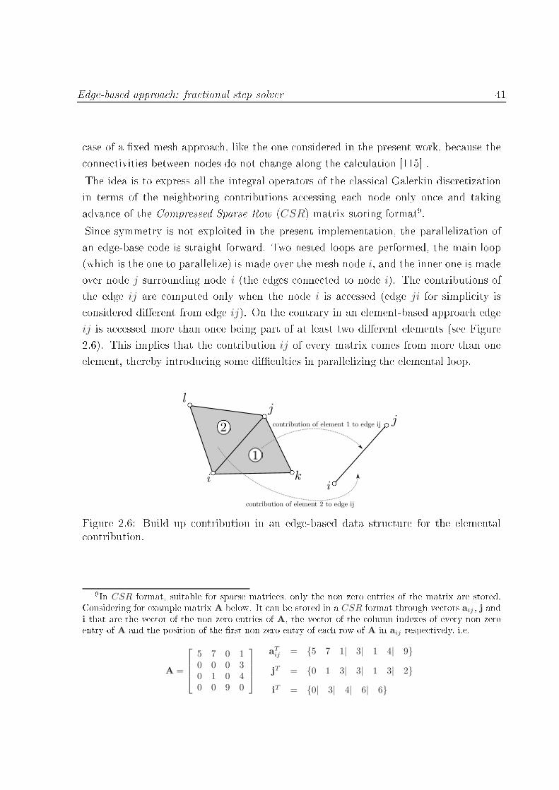
Edge-based approa h: fra tional step solver 41 ase of a xed mesh approa h, like the one onsidered in the present work, be ause the onne tivities between nodes do not hange along the al ulation [115 .The idea is to express all the integral operators of the lassi al Galerkin dis retizationin terms of the neighboring ontributions a essing ea h node only on e and takingadvan e of the Compressed Sparse Row (CSR) matrix storing format9.Sin e symmetry is not exploited in the present implementation, the parallelization ofan edge-base ode is straight forward. Two nested loops are performed, the main loop(whi h is the one to parallelize) is made over the mesh node i, and the inner one is madeover node j surrounding node i (the edges onne ted to node i). The ontributions ofthe edge ij are omputed only when the node i is a essed (edge ji for simpli ity is onsidered dierent from edge ij). On the ontrary in an element-based approa h edgeij is a essed more than on e being part of at least two dierent elements (see Figure2.6). This implies that the ontribution ij of every matrix omes from more than oneelement, thereby introdu ing some di ulties in parallelizing the elemental loop.

Figure 2.6: Build up ontribution in an edge-based data stru ture for the elemental ontribution.9In CSR format, suitable for sparse matri es, only the non zero entries of the matrix are stored.Considering for example matrix A below. It an be stored in a CSR format through ve tors aij , j andi that are the ve tor of the non zero entries of A, the ve tor of the olumn indexes of every non zeroentry of A and the position of the rst non zero entry of ea h row of A in aij respe tively, i.e.

A =

5 7 0 10 0 0 30 1 0 40 0 9 0

aTij = 5 7 1| 3| 1 4| 9

jT = 0 1 3| 3| 1 3| 2

iT = 0| 3| 4| 6| 6

42 The uid problem2.5.1 Stabilized formulationAs already mentioned in Se tion 2.4.1 in the edge-based approa h, as well as in theelement-based one, SGS methods are employed to stabilize equations 2.39. In the presentwork the Orthogonal sub-grid s ale OSS method introdu ed by Codina [34, 38 is used.In this ase the spa e for the sub-grid s ale is taken orthogonal to the nite element one.Following stri tly the operations outlined in [39, 41, 115, the problem already presentedin equation 2.39, with the insertion of the onve tion and in ompressibility stabilizationterms, is: nd (uh, ph,πh, ξh) in Vh ×Qh × Vh × Vh su h that∫

Ω

wh∂tuhdΩ +

∫

Ω

whuh · ∇uhdΩ

−∫

Ω

nph(∇ ·wh)dΩ + 2

∫

Ω

∇wh : ν∇uhdΩ

+

∫

Ω

wh(E1uh + E2|uh|uh)dΩ−∫

Ω

whnbdΩ

−∫

Ω

τ(uh · ∇wh)Ph⊥(uh · ∇uh + E2|uh|uh)dΩ = 0 ∀wh ∈ Vh;

∫

Ω

qh∇ · uhdΩ+

∫

Ω

τ∇qhPh⊥(n∇ph)dΩ = 0 ∀qh ∈ Qh;

(2.67)where Ph

⊥ is the spa e of orthogonal proje tions Ph⊥ = I − Ph and Ph is the L2 −

projection onto Vh. That isPh

⊥(uh · ∇uh + E2|uh|uh) = uh · ∇uh + E2|uh|uh − πh; (2.68a)Ph

⊥(∇ph) = n∇ph − ξh; (2.68b)with πh and ξh dened as∫

Ω

whπhdΩ =

∫

Ω

wh(uh · ∇uh + E2|uh|uh)dΩ; ∀wh ∈ Vh (2.69a)∫

Ω

whξhdΩ =

∫

Ω

whn∇phdΩ; ∀wh ∈ Vh (2.69b)The additional unknowns ξ and π an be easily expressed in fun tion of velo ity andpressure through this equations.Remark 8. A split-OSS is implemented. The orre t form of applying OSS to themomentum equation would be to onsider a stabilization term like equation 2.45 where

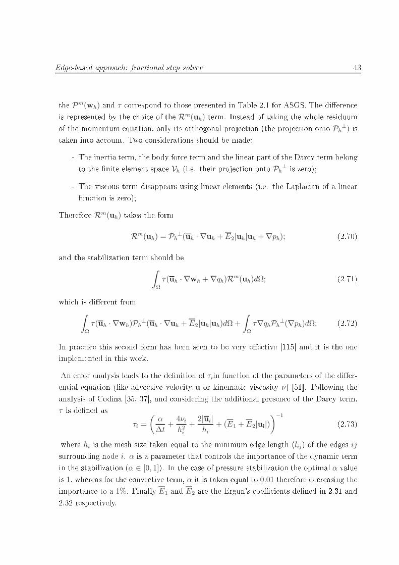
Edge-based approa h: fra tional step solver 43the Pm(wh) and τ orrespond to those presented in Table 2.1 for ASGS. The dieren eis represented by the hoi e of the Rm(uh) term. Instead of taking the whole residuumof the momentum equation, only its orthogonal proje tion (the proje tion onto Ph⊥) istaken into a ount. Two onsiderations should be made:- The inertia term, the body for e term and the linear part of the Dar y term belongto the nite element spa e Vh (i.e. their proje tion onto Ph

⊥ is zero);- The vis ous term disappears using linear elements (i.e. the Lapla ian of a linearfun tion is zero);Therefore Rm(uh) takes the formRm(uh) = Ph

⊥(uh · ∇uh + E2|uh|uh +∇ph); (2.70)and the stabilization term should be∫

Ω

τ(uh · ∇wh +∇qh)Rm(uh)dΩ; (2.71)whi h is dierent from∫

Ω

τ(uh · ∇wh)Ph⊥(uh · ∇uh + E2|uh|uh)dΩ +

∫

Ω

τ∇qhPh⊥(∇ph)dΩ; (2.72)In pra ti e this se ond form has been seen to be very ee tive [115 and it is the oneimplemented in this work.An error analysis leads to the denition of τiin fun tion of the parameters of the dier-ential equation (like adve tive velo ity u or kinemati vis osity ν) [51. Following theanalysis of Codina [35, 37, and onsidering the additional presen e of the Dar y term,

τ is dened asτi =

(α

∆t+

4νih2i

+2|ui|hi

+ (E1 + E2|ui|))−1 (2.73)where hi is the mesh size taken equal to the minimum edge length (lij) of the edges ijsurrounding node i. α is a parameter that ontrols the importan e of the dynami termin the stabilization (α ∈ [0, 1]). In the ase of pressure stabilization the optimal α valueis 1, whereas for the onve tive term, α it is taken equal to 0.01 therefore de reasing theimportan e to a 1%. Finally E1 and E2 are the Ergun's oe ients dened in 2.31 and2.32 respe tively.

44 The uid problem2.5.2 Dis retization pro edureSystem 2.67 an be rewritten in a semi dis rete form asM∂tu+ KC (u)u− Gp+ Kµu+ KD (u)u+ Suu− Sππ − F = 0; (2.74a)

Du+ Spp− Sξξ = 0; (2.74b)Mπ − KC(u)u = 0; (2.74 )

Mξ − ∇p = 0; (2.74d)where u is the ve tor of nodal velo ities and p the ve tor of nodal pressures. Theoperators take the form presented in Table 2.4 and the stabilization operators Si aredened as shown in Table 2.5.In order to simplify the problem, equations 2.74 and 2.74d an be substituted inequations 2.74a and 2.74b respe tively, givingM∂tu+ KC (u)u− Gp+ Kµu

+KD (u)u+ Suu− SπM−1KC(u)u− F = 0; (2.75a)Du+ Spp− SξM−1

∇p = 0; (2.75b)The residual of the momentum equations without the dynami term is dened asr (u,p) := KC (u)u− Gp+ Kµu

+KD (u)u+ Suu− SπM−1KC(u)u− F;

(2.76)Remark 9. The tilde super-index over the matrix operators emphasizes the dieren ebetween the same operators in the element-based formulation presented in Table 2.2.

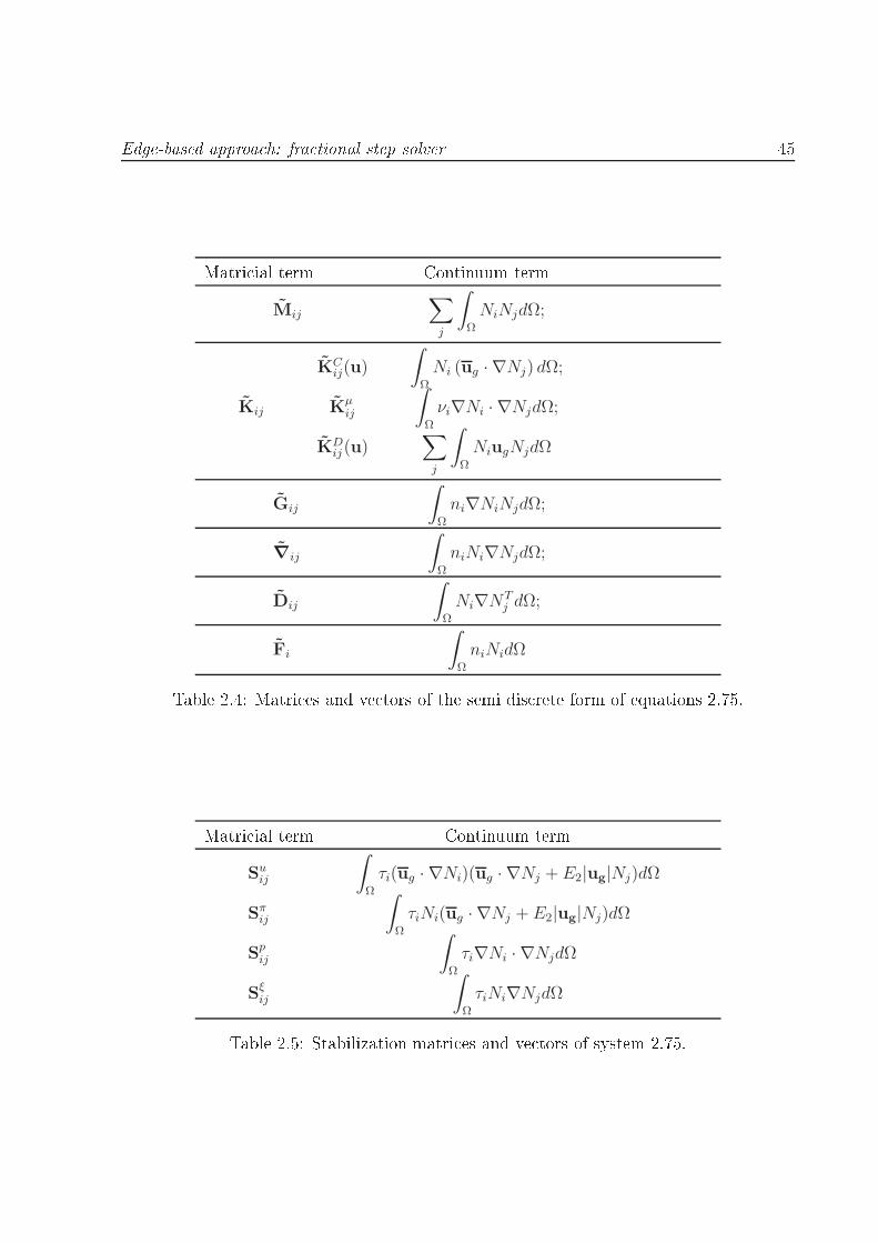
Edge-based approa h: fra tional step solver 45Matri ial term Continuum term

Mij

∑

j

∫

Ω

NiNjdΩ;

KCij(u)

∫

Ω

Ni (ug · ∇Nj) dΩ;

Kij Kµij

∫

Ω

νi∇Ni · ∇NjdΩ;

KDij (u)

∑

j

∫

Ω

NiugNjdΩ

Gij

∫

Ω

ni∇NiNjdΩ;

∇ij

∫

Ω

niNi∇NjdΩ;

Dij

∫

Ω

Ni∇NTj dΩ;

Fi

∫

Ω

niNidΩTable 2.4: Matri es and ve tors of the semi dis rete form of equations 2.75.Matri ial term Continuum term

Suij

∫

Ω

τi(ug · ∇Ni)(ug · ∇Nj + E2|ug|Nj)dΩ

Sπij

∫

Ω

τiNi(ug · ∇Nj + E2|ug|Nj)dΩ

Spij

∫

Ω

τi∇Ni · ∇NjdΩ

Sξij

∫

Ω

τiNi∇NjdΩTable 2.5: Stabilization matri es and ve tors of system 2.75.

46 The uid problem2.5.3 Fra tional step solver using an expli it 4th order RungeKutta time s hemeThe modied form of the Navier-Stokes equations are solved using a fra tional step algo-rithm. Pressure-splitting approa hes of the fra tional-step type are very onvenient dueto their high omputational e ien y for ows at high Re, and have enjoyed widespreadpopularity sin e the original works of Chorin [33 and Temam [119. The fundamentalidea is to solve the momentum equation keeping xed the pressure and later orre tingthe pressure so as to guarantee the satisfa tion of the divergen e onstraint. A modernalgebrai presentation of the method an be found in [36. The fra tional step approa his traditionally presented in an impli it ontext, typi ally using a rst or se ond orderBa kward Dierentiation Formula (BDF1 or BDF2 algorithm respe tively) for the timeintegration of the momentum equation. In dealing with free-surfa e problems unfortu-nately, the shape of the uid domain, and onsequently the boundary onditions on thefree surfa e, are subje ted to frequent and radi al hanges. This implies that, to allowa satisfa tory representation of the solution, an a urate tra king should be performed.In pra ti e, it is typi ally observed that, even fully impli it s hemes are pra ti ally lim-ited to time steps for whi h the free surfa e approximately moves of one element lengthper time step. Su h heuristi onstraint is equivalent in essen e, to a restri tion onthe pra ti al CFL (Courant Friedri hs Lewy)10 number to values in the order of unity.This observation ee tively implies that expli it s hemes will be ompetitive providedthat CFL ≈ 1 an be used and meshes of su iently good quality an be generated.This motivates the use of an expli it form of the fra tional step s heme (see for example[109) based on the use of a 4th order Runge Kutta (RK4) in dealing with the momentumequation.Before pro eeding in the des ription of the method, it should be observed that thealgebrai splitting proposed by Codina in [36 leads naturally to the denition of a dis- rete Lapla ian DM−1G whi h in prin iple does not introdu e any additional error inthe imposition of the divergen e freeness ondition with respe t to the original mono-lithi s heme. However, in pra ti e the use of the dis rete Lapla ian implies a large10The CFL, for hyperboli system of partial dierential equations (PDEs), is dened byCFL =

λmax · dth

; (2.77)where λmax is the maximum eigenvalue of the system, dt the time step and h the size of the element[81, 109.

Edge-based approa h: fra tional step solver 47 omputational burden as the matrix is rather densely populated. In order to over omesu h problem the dis rete Lapla ian is typi ally substituted by a ontinuum Lapla ianwhi h has a mu h smaller sten il than the dis rete one (around six times smaller in3D). This fa t has important onsequen es both on the e ien y and on the stabilityof the numeri al s heme (see e.g. [36) but in parti ular it has an important impa t onthe mass onservation properties of the method [66. One pra ti al issue is that whilethe use of a dis rete Lapla ian matrix guarantees an invertible matrix, this is not the ase when the ontinuum form is hosen implying that pressure needs to be xed on theNeumann boundary, that is, pressure is to be imposed strongly, at least for the solutionof the pressure step. This implies that when FS is to be used the pressure is knownbeforehand on the Neumann boundary.Given su h situation, it is onvenient, to avoid integrating by parts the pressure gradientterm, using the equivalent formula

∫

Ω

w · ∇pdΩ = −∫

Ω

p∇ ·wdΩ+

∫

∂Ω

w · pndΓ (2.78)This implies that the pressure spa e should be in [H1(Ω)]d whi h is an additional re-quirement to the smoothness of the fun tion. Su h modied form has the importantadvantage that no boundary integrals need to be omputed (se ond integral of the rightand side of equation 2.78) for the pressure whi h leads to an easier appli ation of thepressure boundary ondition on the free surfa e as it will be explained in Se tion 2.6.4.This onsideration leads to the following expression for the residual at node i (note theuse of ∇ instead of G).r (u,p) := KC (u)u+ ∇p+ Kµu

+KD (u)u+ Suu− SπM−1KC(u)u− F;

(2.79)Remark 10. Using Eq. 2.78 implies a pointwise appli ation of the normal for e on theNeumann boundary instead of its weak imposition. This is an a eptable approximationfor low vis osity ows for whi h the term ∫

Ωn · µ∆udΩ is negligible.On the basis of su h denition the time integration an now be performed.

48 The uid problemRunge Kutta time integration s hemeThe lower omputational ost of an expli it time integration te hnique (that does notrequire solving of a system of equations), is not the only advantage of this approa h. Itsimplementation is highly parallelizable, whi h is the main reason why it has been hosenin this work. Moreover onsidering the m-Runge Kutta s hemes, it is known that theorder of the time integration an be arbitrarily hosen, although they give m− th orderof a ura y up to m = 4 [51. Whenever for m > 4 the order is lower than m. That isthe reason of the popularity of the 4-steps s heme (RK4).It is demonstrated that the RK4 is the optimal ompromise between the number ofintermediate steps and the permissible time step size in spite of its onditional stability.For more details the onsultation of [51 is re ommended.RK4 makes use of the solution at tn to evaluate the solution at time tn+1 by al ulatingthe residual of the equations at a ertain number of intermediate steps.This means that for a general Cau hy problem∂y

∂t= f(y(t), t); (2.80)a one step expli it approa h leads to a time s heme with the following general format

yn+1 − yn

∆t= f(yn, tn); (2.81)whereas for the 4th order Runge Kutta method

yn+1 − yn

∆t=

1

6(r1 + 2 r2 + 2 r3 + r4); (2.82)where ri with i = 1, 2, 3, 4 are the residuals of the stationary form of 2.80 evaluated at

r1 = f (tn, yn) ;

r2 = f

(

tn +∆t

2, yn +

∆t

2· r1)

;

r3 = f

(

tn +∆t

2, yn ++

∆t

2· r2)

;

r4 = f (tn +∆t, yn +∆t · r3) .

(2.83)

Edge-based approa h: fra tional step solver 49In order to fully explain every stage of the integration s heme applied to the momentumequation let us use the denition of the stabilized residual obtained in equation 2.79.The semi-dis rete form of the momentum equations in terms of the residuals at theintermediate stages is thenM

un+1 − un

∆t=

1

6[r1 + 2 r2 + 2 r3 + r4];

=1

6

[r(un,pn) + 2 r(uθ1,pθ1) + 2 r(uθ2,pθ2) + r(uθ3,pθ3)

];

(2.84)where r(uθi ,pθi) are the residuals of the momentum equations dened by equation 2.79evaluated at θi intermediate stages.To orre tly evaluate the residual at ea h intermediate time step, the solution of the ontinuity equation would have been required. This would have onsiderably redu edthe e ien y requiring a huge omputational eort. In order to over ome this issue,a ording to [111, a linear variation of pressure is assumed in the time step. It shouldbe remarked that this assumption leads the velo ity eld to be divergen e free only atthe end of the step.Redening equation 2.79 asr(u,p) = ru(u) + rp(p); (2.85)being ru(u) the part of the residual related to velo ity and rp(p) the part related tothe pressure gradients. The residuals be ome

r1 := r(un,pn) = ru(un) + ∇pn;

r2 := r(uθ1,pθ1) = ru(uθ1) +1

2

(

∇pn + ∇pn+1

)

;

r3 := r(uθ2,pθ2) = ru(uθ2) +1

2

(

∇pn + ∇pn+1

)

;

r4 := r(uθ3,pθ3) = ru(uθ3) + ∇pn+1;

(2.86)And the global momentum equation 2.84 an be symboli ally rewritten as

50 The uid problemM

un+1 − un

∆t=

1

6

[ru(un) + 2 ru(uθ1) + 2 ru(uθ2) + ru(uθ3)

]

+1

2

[

∇pn + ∇pn+1

](2.87)Final system using a fra tional step approa h and a RK4In order to de ouple the solution for the velo ity and pressure, the traditional pressuresplitting pro edure is performed and the fra tional step velo ity u is inserted. This gives

Mu− un

∆t=

1

6

[ru(un) + 2 ru(uθ1) + 2 ru(uθ2) + ru(uθ3)

]+

1

2∇pn; (2.88a)

Mun+1 − u

∆t+

1

2∇(pn+1 − pn) = 0; (2.88b)

Dun+1 + Sppn+1 − SξM−1Gpn+1 = 0; (2.88 )where it has to be remarked that equation 2.88a only depends on the pressure at theprevious time step and on the intermediate fra tional step velo ities, leading to a slightlydierent RK4 steps as explained later on.From equation 2.88bun+1 = u− ∆t

2M−1

∇(pn+1 − pn); (2.89)that substituted in equation 2.88 givesDu− ∆t

2DM−1

∇(pn+1 − pn) + Sppn+1 − SξM−1Gpn+1 = 0. (2.90)Finally substituting the dis rete Lapla ian (DM−1∇) by the ontinuous one (L), thenal system to be solved is [109:

Mu− un

∆t=

1

6

[ru(un) + 2 ru(uθ1) + 2 ru(uθ2) + ru(uθ3)

]+

1

2∇pn; (2.91a)

∆t

2L(pn+1 − pn

)= Du+ Sppn+1 − SξM−1Gpn+1; (2.91b)

un+1 = u− ∆t

2M−1

∇(pn+1 − pn

); (2.91 )

Edge-based approa h: fra tional step solver 51where the residuals of equation 2.91a are evaluated a ording to the following stepsru(un); (2.92a)uθ1 = un + M−1∆t

2

[

ru(un) + ∇pn]

; (2.92b)ru(uθ1); (2.92 )uθ2 = un + M−1∆t

2

[

ru(uθ1) +1

2∇pn

]

; (2.92d)ru(uθ2) (2.92e)uθ3 = un + M−1∆t

[

ru(uθ2) +1

2∇pn

]

; (2.92f)ru(uθ3); (2.92g)2.5.4 The edge-based operatorsHaving made the hoi e of using an expli it s heme for the time integration of themomentum equation, a suitable data stru ture for the fast al ulation of the residualsshould be devised. The idea to be exploited is that many of the integrals involved in the omputation of the residual an be written in terms of onstant operators whi h an bedire tly applied to the nodal values. Dierent te hniques were developed over the yearsto rea h su h goal. In writing this work the nodal-based approa h des ribed in [34 isblended with the edge-based proposed in [81, 115.The starting point is the systemati usage of the partition-of-unity property of the FEshape fun tions, whi h provides the relations∑

i

Ni = 1 =⇒ Ni = 1−∑

j 6=i

Nj ; (2.93)and, as a onsequen e,∑

i

∇Ni = 0 =⇒ ∇Ni = −∑

j 6=i

∇Nj. (2.94)The edge-based approa h is obtained by applying systemati ally su h relations for the omputation of the dis rete operators of interest.In the following the dierent terms involved in the al ulation of the residual are on-sidered one by one, by expressing the ontributions to the entry orresponding to a given

52 The uid problemnode i. The j index indi ates one of the neighbor nodes of i whi h share an edge withit.Gradient term. The gradient term (not integrated by parts) whi h appears in themomentum equation, reads

∑

j

∫

Ω

Ni∇NjpjdΩ =∑

j 6=i

∫

Ω

Ni∇NjpjdΩ +

∫

Ω

Ni∇NipidΩ

=∑

j 6=i

∫

Ω

Ni∇NjpjdΩ−∫

Ω

Ni

(∑

j 6=i

∇Nj

)

pidΩ

=∑

j 6=i

∫

Ω

Ni∇Nj (pj − pi) dΩ

=∑

j 6=i

∇ij (pj − pi).

(2.95)Applying equation 2.94 it an be demonstrated that the pressure gradient term an be omputed by using the ∇ij for any edge ij. Note that the term ii is never needed withthe approa h proposed.Divergen e term. The derivation of the divergen e term is basi ally identi al tothe previous one, with the only dieren e that a s alar produ t is involved. Followingexa tly the same steps as before it an be readily shown that

∑

j

Dij · uj =∑

j 6=i

Dij · (uj − ui) dΩ. (2.96)Conve tion term. The non-linear onve tion term has to be approximated to twithin the framework of the present edge based formulation. Several possibilities existto obtain a suitable form to be used in the al ulations. One ould start by onsidering

Edge-based approa h: fra tional step solver 53the onservative form of the onve tion operator ∇ · (u⊗ u) .∑

j

∫

Ω

Ni∇Nj · (uj ⊗ uj) dΩ =

=∑

j 6=i

∫

Ω

Ni∇Nj · ujujdΩ−∫

Ω

Ni

(∑

j 6=i

∇Nj

)

· uiuidΩ;

(2.97)whi h tells us that the onve tive term an be estimated as

∑

j 6=i

(

∇ij · uj

)

uj −∑

j 6=i

(

∇ij · ui

)

ui. (2.98)Alternatively, one an start with the non- onservative form of the same equation anduse a nodal integration rule as proposed in [34. This approa h estimates the onve tiveterm ontribution as∑

j 6=i

(

∇ij · ui

)

(uj − ui) . (2.99)The rst approa h is globally onservative by onstru tion in the sense that the sumover all of the nodes in the mesh is guaranteed to give zero. This property is onlyapproximately veried by the se ond te hnique, sin e the integration rule is not exa t.In pra ti e, both approa hes work ee tively. Nevertheless the se ond approximationappears to be slightly more robust and was the one hosen in that work.Weak gradient term. The migration from a lassi al nite element to an edge-based implementation requires des ribing the gradient of a s alar fun tion integrated byparts. Sin e in the urrent formulation the pressure gradient term is not integrated byparts, this is not stri tly needed for the implementation of the present method. In any ase, following [86∑

j

∫

Ω

ni∇NiNjpj =∑

j 6=i

∫

Ω

ni∇NiNjpjdΩ+

∫

Ω

ni∇NiNipidΩ

=∑

j 6=i

∫

Ω

ni∇NiNjpjdΩ−∫

Ω

(∑

j 6=i

ni∇Nj

)

NipidΩ

= Gijpj − ∇ijpi.

(2.100)

54 The uid problemVis ous term. The vis ous term in the Navier-Stokes equations requires estimatingthe s alar Lapla ian operator Lij . Although the possibility exists of storing dire tly onea h edge an entry of the type Lij :=∫

Ω∇Ni ·∇NjdΩ, in the present work it is preferredto store a matrix term of the type

Ldij =

∫

Ω

∇Ni ⊗∇NjdΩ; (2.101)on ea h edge of the mesh. The s alar gradient an then be obtained as needed by thetra e operator asLij = Tr

(Ld

ij

); (2.102)whi h allows writing the vis ous term as

∑

i 6=j

Tr(Ld

ij

)µ (uj − ui) (2.103)Spe ial terms. The terms des ribed until now in lude all of the terms that areneeded for the implementation of the Navier-Stokes equations. Nevertheless, it is appro-priate to remark that storing the matrix Lapla ian Ld

ij instead of its s alar ounterpart,is justied for the implementation of the stabilization operators. A detailed des riptionof the use of Ldij in this ontext an be found in [83. The need for storing su h operator an be also understood by onsidering a SUPG-like stabilization operator. On a givennode i, the stabilization operator has the form

∑

i 6=j

∇ · (ui ⊗ ui)∇ (uj − ui) . (2.104)By using the matrix lapla ian operator, this an be approximated as∑

i 6=j

(ui · Ld

ij · ui

)∇ · (uj − ui) ; (2.105)whi h requires onsidering Ld

ij in the omputation. Similarly, the matrix form is alsouseful in the omputation of the sub-s ale residuals and for the denition of a ross-winddissipation term whi h is useful for ontrolling unwanted numeri al os illations.Remark 11. The ommon features of all of the terms des ribed is that they an beevaluated for ea h node i independently of all of the others. This implies that the

Edge-based approa h: fra tional step solver 55 al ulation of the residuals an be performed in parallel for ea h node of the mesh.Remark 12. All the other magnitudes that have not been spe i ally treated here aretaken as nodal, su h as, for instan e, the intrinsi time τ .2.5.5 Improving mass onservationIndependently on the time a ura y of the numeri al s heme used for the rst step, theoverall s heme an not be more than se ond order a urate due to the pressure splittingpro edure. Furthermore, the use of the ontinuum Lapla ian operator, mandatory in the ontext of a semi-expli it s heme, implies some volume loss parti ularly on entratedin the vi inity of the free surfa e (Neumann boundary). The origin of su h loss an betra ed ba k to two distin t phenomena:1. As observed in [66, the pressure is xed on the Neumann boundary as this isneeded to make the Lapla ian resolvable. This implies that it loses the apa ityto adapt lo ally so to attempt guaranteeing the lo al mass onservation.2. The divergen e onstraint (Du = 0) is generally evaluated at time step n + 1implying that it depends ex lusively on the velo ity at n + 1. Any error in thefulllment of this onstraint at the pre eding step (Dun = 0 ) is simply dis ardedand never re overed.The algorithm devised for the solution of the free surfa e problem attempts to minimizethe rst issue. The idea, as shown in Se tion 2.6.4, is that the pressure will be xedon the nodes outside the free surfa e, thus letting some freedom to the nodes in itsproximity.On the other hand, the fulllment of the divergen e free ondition at the present timestep (n+1) and at the previous one (n) are ombined in order to over ome the drawba kstated in point 2. The idea is the following: if no error was made in the past, it an bestated that Dun = 0. However this assumption is not veried in pra ti e and volume iseither reated or destru ted at a rate of Dun. While usually this information is simplydis arded, in the present work the divergen e free ondition (Dun+1 = 0) is modied inorder to sum up the volume variation lost (or gained) at the previous time (Dun).In mathemati al terms the proposal is simply to modify the divergen e onstraint asDun+1 +Dun = 0 (2.106)

56 The uid problemAs shown in some of the examples, this simple modi ation improves the volume on-servation of the overall s heme.2.6 Free surfa e tra king. The Level Set methodThe proposed te hnique is based on the use of a xed-grid approa h. Hen e at ea htime step the uid domain should be dened, implying:1. The denition of a tra king method that allows:- moving the uid free surfa e;- dening the position of the uid boundary at ea h time step;2. The appli ation of the boundary onditions at the uid boundary that do notne essarily oin ide with mesh edges;A level set te hnique is employed to fa e the rst issue. The level set method was on eived as a methodology to following moving interfa es. The moving boundaries are omposed of the zero-valued iso-surfa e of a given smooth fun tion (at least Lips hitz ontinuous11 [11) ϕ(x, t).Let us all Ω0 ⊂ Rd (where d is the spa e dimension) the global ontrol domain ofanalysis. The uid domain dened in the previous se tion at time t is Ω(t) ⊂ Ω0. Theboundary of Ω(t) is dened by part of ∂Ω0 and by a moving boundary dened as

∂Ωm(t) := x | ϕ(x, t) = 0 (2.107)From now on Ω(t) = Ω, and Ωm(t) = Ωm and the expli it indi ation of time will beomitted for simpli ity. Following the same riteria, the uid domain at a given timestep tn is Ω(tn) = Ωn.11In mathemati s Lips hitz ontinuity is a stronger requirement than simple ontinuity onditioningthe speed of hange of the fun tion. Let f : Rm → Rm. Given an open set B ⊆ R

m, f is Lips hitz- ontinuous on the open subset B if there exists a onstant Λ ∈ R+

0su h that

||f(x)− f(y)|| ≤ Λ||x− y|| ∀x,y ∈ B.

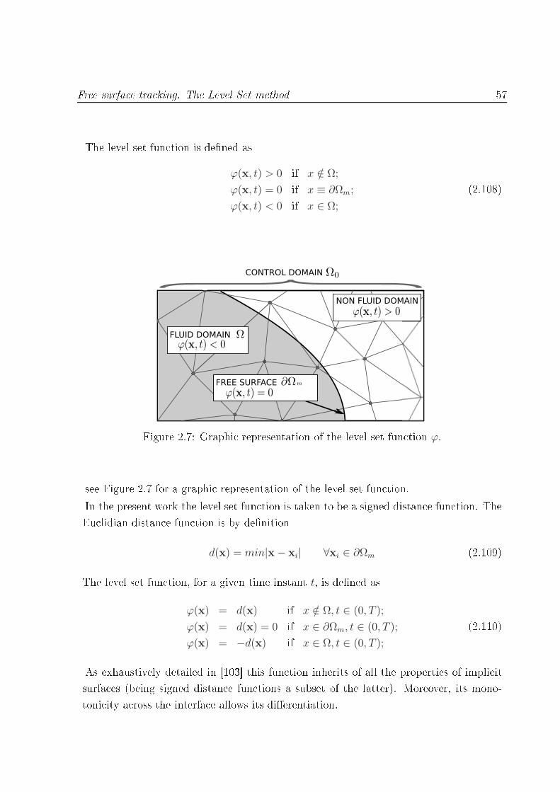
Free surfa e tra king. The Level Set method 57The level set fun tion is dened asϕ(x, t) > 0 if x /∈ Ω;

ϕ(x, t) = 0 if x ≡ ∂Ωm;

ϕ(x, t) < 0 if x ∈ Ω;

(2.108)

FLUID DOMAIN

FREE SURFACE

NON FLUID DOMAIN

CONTROL DOMAIN

mFigure 2.7: Graphi representation of the level set fun tion ϕ.see Figure 2.7 for a graphi representation of the level set fun tion.In the present work the level set fun tion is taken to be a signed distan e fun tion. TheEu lidian distan e fun tion is by denitiond(x) = min|x− xi| ∀xi ∈ ∂Ωm (2.109)The level set fun tion, for a given time instant t, is dened as

ϕ(x) = d(x) if x /∈ Ω, t ∈ (0, T );

ϕ(x) = d(x) = 0 if x ∈ ∂Ωm, t ∈ (0, T );

ϕ(x) = −d(x) if x ∈ Ω, t ∈ (0, T );

(2.110)As exhaustively detailed in [103 this fun tion inherits of all the properties of impli itsurfa es (being signed distan e fun tions a subset of the latter). Moreover, its mono-toni ity a ross the interfa e allows its dierentiation.

58 The uid problemThe fundamental idea of using the level set approa h an now be understood onsideringthe mass onservation equation for a variable-density uid:dρ

dt+ u · ∇ρ+ ρ∇ · u = 0 (2.111)The ase of interest is that ρ 6= 0 inside the uid domain and ρ = 0 outside the freesurfa e, where a regularization fun tion should be onsidered to be applied to ρ to makeit dierentiable in spa e.Let us split equation 2.111 in the following two equationsdρ

dt+ u · ∇ρ = 0 (2.112)and

ρ∇ · u = 0→∇ · u = 0 (2.113)It is easy to understand that if su h two equations are veried equation 2.111 will alsobe veried. This requirement is in fa t stri ter the the original one. Now, equation 2.112represents the transport of the density with the mean ow velo ity. Sin e the density an be rather badly behaved as it approximates a jump, it is onvenient to repla e itby the transport of a smooth s alar ϕ (in the present work ϕ is the distan e fun tion)whi h an be used to re over the density distribution at any moment. The problem isthus transferred to the solution of the transport problem∂tϕ+ u · ∇ϕ = 0 in Ω0, t ∈ (0, T ),

ϕ = ϕ on ∂Ωin, t ∈ (0, T ),

ϕ(x, 0) = ϕ0(x) in Ω0,

(2.114)where ∂Ωin := x ∈ ∂Ω0 | u ·n < 0 is the inow part of ∂Ωm. When the uid entersthe porous matrix an a eleration of the advan ing front an be observed be ause of arestri tion of the empty area. This is taken into a ount by onsidering the adve tivevelo ity equal to the a tual uid velo ity dened in equation 2.2.Two dierent solution approa hes are used for the edge-based and the element-basedalgorithm for the solution of the onve tive system 2.114. In the edge-based te hnique a4th order Runge Kutta s heme 2.114 is implemented and an OSS stabilization te hniqueis used, similarly to what has already been explained in Se tion 2.5.1. Conversely a

Free surfa e tra king. The Level Set method 59Crank-Ni olson time integration s heme is employed in the element-based approa hstabilized with the ASGS method.2.6.1 Coupling the level set equation and the Navier-StokessolverIn order to ompletely dene the approa h used in this work, the des ription of the oupling between the Navier-Stokes solver and the newly added level set equations isneeded. Con eptually, the velo ity obtained from the solution of the Navier-Stokesequation has to be used in onve ting ϕ, while the zero level set fun tion providesthe position of the free-surfa e and is onsequently needed to pres ribe the pressure ondition on the Neumann boundary. Many dierent approa hes have been proposedover the years to perform su h oupling; some based on sub-integration te hniques on the ut elements [42 and others based on some form of regularization for the density fun tionin the vi inity of the free surfa e. The proposal in this work rises from the observationthat, on e a ontinuous pressure distribution is assumed, only the gradient of the existingpressure appears in the momentum equation (as already observed before,the pressureterm is not integrated by parts). This implies that the momentum equation an be solvedapproximately without knowing exa tly the position of the free surfa e, provided thatan estimate of the pressure gradient is given in any a tive (or potentially a tive) areaof the uid domain. On the other hand, the imposition of the zero tra tion onditionon the Neumann boundary ould be applied in the pressure orre tion step through theimposition of adapt boundary onditions at the level of the pressure Lapla ian system.To omplete the algorithm some other ingredients are needed:- An extrapolation fun tion to dene the values of the velo ity on a band ontainingthe free surfa e of the uid and to allow the imposition of the in ompressibility ondition on the free surfa e;- A tool for al ulating the nodal distan es in the whole domain Ω0;- A method to impose the boundary onditions on the free surfa e.2.6.2 The extrapolation pro edureIn order to allow the onve tion of the free surfa e ∂Ωm in regions of Ω0 out of Ωn , anextrapolation of the velo ity eld in the part of the domain lose to the free surfa e but

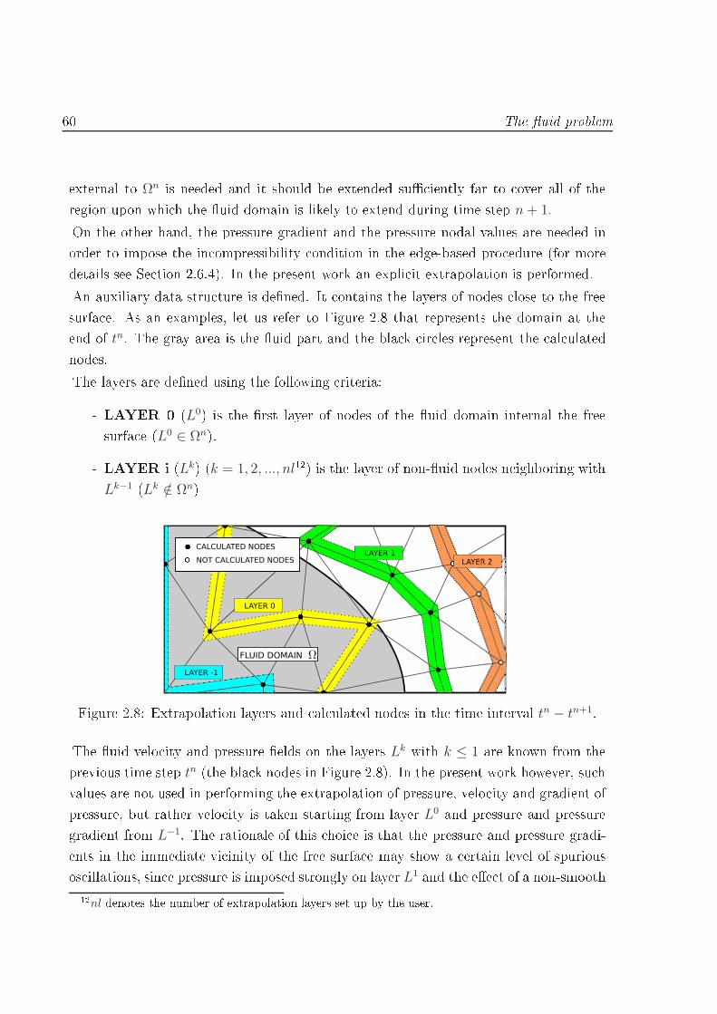
60 The uid problemexternal to Ωn is needed and it should be extended su iently far to over all of theregion upon whi h the uid domain is likely to extend during time step n+ 1.On the other hand, the pressure gradient and the pressure nodal values are needed inorder to impose the in ompressibility ondition in the edge-based pro edure (for moredetails see Se tion 2.6.4). In the present work an expli it extrapolation is performed.An auxiliary data stru ture is dened. It ontains the layers of nodes lose to the freesurfa e. As an examples, let us refer to Figure 2.8 that represents the domain at theend of tn. The gray area is the uid part and the bla k ir les represent the al ulatednodes.The layers are dened using the following riteria:- LAYER 0 (L0) is the rst layer of nodes of the uid domain internal the freesurfa e (L0 ∈ Ωn).- LAYER i (Lk) (k = 1, 2, ..., nl12) is the layer of non-uid nodes neighboring withLk−1 (Lk /∈ Ωn)

LAYER 0

LAYER 1

LAYER 2

CALCULATED NODES

NOT CALCULATED NODES

LAYER -1

FLUID DOMAINFigure 2.8: Extrapolation layers and al ulated nodes in the time interval tn − tn+1.The uid velo ity and pressure elds on the layers Lk with k ≤ 1 are known from theprevious time step tn (the bla k nodes in Figure 2.8). In the present work however, su hvalues are not used in performing the extrapolation of pressure, velo ity and gradient ofpressure, but rather velo ity is taken starting from layer L0 and pressure and pressuregradient from L−1. The rationale of this hoi e is that the pressure and pressure gradi-ents in the immediate vi inity of the free surfa e may show a ertain level of spuriousos illations, sin e pressure is imposed strongly on layer L1 and the ee t of a non-smooth12nl denotes the number of extrapolation layers set up by the user.

Free surfa e tra king. The Level Set method 61pressure boundary ondition may be still felt on layer L0. The extrapolation of pressure(and pressure gradient) is thus started from the inner layer (L−1), whi h guarantees amu h smoother behavior of the extrapolation area.In symbols, we dene the pressure gradient on ea h node i of a given layer k, as thearithmeti average (avg) of all of its neighbors j whi h belong to the layer of lower order,i.e.∇pki := avg

(∇pk−1

j

)∀k = 0...nl i ∈ Lk j ∈ Lk−1 (2.115)Given su h pressure gradients, pressure is then evaluated on node i so as to maintainthe extrapolated pressure gradient, that is

pki := avg(pk−1j + hij · ∇pk−1

j

)∀k = 0...nl i ∈ Lk j ∈ Lk−1 (2.116)where hij := xj − xi is the ve tor from i to j.The extrapolation of the velo ity is performed in a very similar way, with the onlydieren e that the extrapolation starts from layer L0, not from L−1 (see Figure 2.8 fora graphi al representation).

uki := avg

(uk−1j

)∀k = 1...nl i ∈ Lk j ∈ Lk−1 (2.117)The extrapolation pro edure des ribed above provides a predi tion of the velo ity andpressure elds that is likely to be found outside of the pressure domain. Su h extrap-olation is performed before onve ting the distan e fun tion, and should be extendedsu iently far to over all of the area upon whi h the uid domain is likely to extend dur-ing the following time step. It should be remarked that the data stru ture that ontainsthe dierent layers should be updated every time the distan e fun tion is onve ted.It is interesting also to observe that the hoi e of using the strong form of the pressuregradients in the momentum equations appears at this point to be bene ial. The ideais that sin e the pressure gradient was not integrated by parts, no boundary integral ofthe pressure is needed on the free surfa e (in the solution of the momentum equation)and the only thing needed on any uid element (in luding the elements ut by thefree surfa e) is the orre t omputation of the pressure gradient, whi h is automati allyavailable on e the pressure is extrapolated as des ribed.Remark 13. The data stru ture that ontains the dierent layers should be updatedevery time the distan e fun tion is onve ted.

62 The uid problemRemark 14. The extrapolation of pressure and pressure gradient is ne essary only inthe edge-based formulation in order to approximately pres ribe the zero pressure ondi-tion on the free surfa e, as it will be explained in Se tion 2.6.4. For the element-basedformulation a virtual sub-splitting is proposed and no pressure gradients are needed.2.6.3 The distan e fun tionOn e the onve tion operation has been performed the level set fun tion is no longer theEu lidean distan e fun tion presented in 2.110. To re over its original nature a tool tore-evaluate the nodal distan e from the new al ulated free surfa e, has been developed.Due to the dynami nature of the analyzed problem, a redenition of the uid domainΩ := x ∈ Ω0 | ϕ(x) ≤ 0 is ne essary at ea h time step. In the present se tion themethodology for the al ulation of the distan e eld is des ribed. The 3D ase is takeninto a ount although the 2D ase has also been implemented. For the al ulation ofthe distan e eld of the domain Ω0, numeri al methods have to be employed be ausethe use of analyti al solution is not trivial. The method proposed by Elias, Martinsand Coutinho (see [56 for more details) is taken as a referen e. It takes its origin fromthe Fast Mar hing Method (FMM), a te hnique, rst developed by Sethian (see [114),for the omputation of the arrival time of a front. In the FMM the Eikonal equation(equation 2.118) is given as a boundary ondition

‖∇T‖ · F = 1; (2.118)where T is the time arrival of the front and F is the speed of the front. That meansthat T (p) is the time arrival of the front to point p. Taking F = 1, T (p) is nothing butthe distan e missed by the front to arrive at the point p. That means thatfun tion T oin ides with the signed distan e fun tion ϕ adopted in the present work.‖∇T‖ = ‖∇ϕ‖;The key idea of Elias and oworkers, that makes the dieren e from the FMM, was theuse of a nite element interpolation for the al ulation of the level set fun tion ϕ(x, t).For ea h element its gradient is then dis retized as follows‖∇ϕe‖ = ‖BTd‖; (2.119)

Free surfa e tra king. The Level Set method 63where dT = (d1, d2, d3, d4) is the ve tor of the nodal distan es of a tetrahedral element,and BB =

1

6Ωel

N1,x N1,y N1,z

N2,x N2,y N2,z

N3,x N3,y N3,z

N4,x N4,y N4,z

is the matrix of the derivatives of the shape fun tions in the three artesian dire tions.Then

ϕ,x

ϕ,y

ϕ,z

=

N1,xd1 +N2,xd2 +N3,xd3 +N4,xd4;

N1,yd1 +N2,yd2 +N3,yd3 +N4,yd4;

N1,zd1 +N2,zd2 +N3,zd3 +N4,zd4;

(2.120)Therefore, equation 2.118, with F ≡ 1 an be written as

(ϕe,x)

2 + (ϕe,y)

2 + (ϕe,z)

2 = 1; (2.121)That means that if the distan e of three over four nodes of a 3D element is known(suppose known d1, d2, d3) the value of d4 an be easily al ulated. Considering thefollowing simpli ation:dx = N1,xd1 +N2,xd2 +N3,xd3;

dy = N1,yd1 +N2,yd2 +N3,yd3;

dz = N1,zd1 +N2,zd2 +N3,zd3;

(2.122)and substituting equation 2.122 into equation 2.121 it results(dx +N4,xd4)

2 + (dy +N4,yd4)2 + (dz +N4,zd4)

2 = 1. (2.123)Equation 2.123 is a se ond order equation where the only unknown is d4. The maximumvalue between the two possible solutions of equation 2.123 will be the solution of theproblem. In the ase of an imaginary solution, it is possible to dene the distan efun tion arriving from another element. If this is not possible, the node will be skippedand the solution will be interpolated at the end of the loop [56.Using a xed mesh approa h the free surfa e will not ne essarily oin ide with a layerof nodes but it will ut the elements. This means that the distan e values of at least

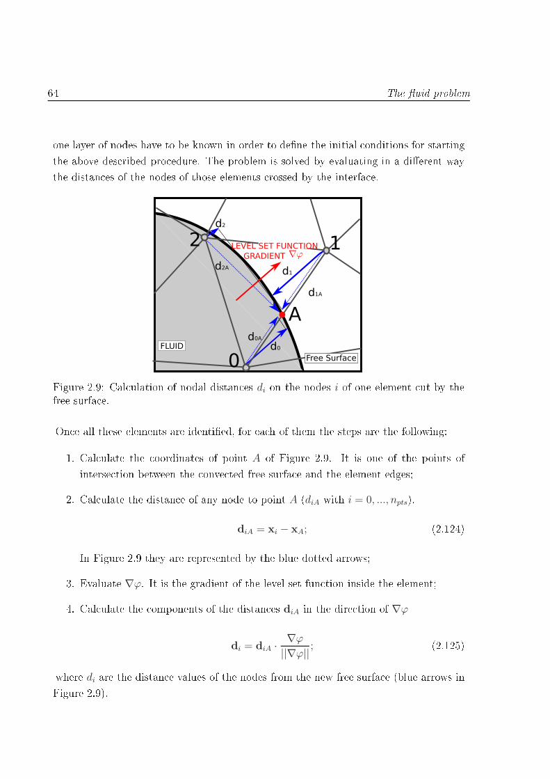
64 The uid problemone layer of nodes have to be known in order to dene the initial onditions for startingthe above des ribed pro edure. The problem is solved by evaluating in a dierent waythe distan es of the nodes of those elements rossed by the interfa e.

A

d1A

d0A

d2A d1

d2

d0

0

12 LEVEL SET FUNCTION

GRADIENT

Free Surface

FLUIDFigure 2.9: Cal ulation of nodal distan es di on the nodes i of one element ut by thefree surfa e.On e all these elements are identied, for ea h of them the steps are the following:1. Cal ulate the oordinates of point A of Figure 2.9. It is one of the points ofinterse tion between the onve ted free surfa e and the element edges;2. Cal ulate the distan e of any node to point A (diA with i = 0, ..., npts).diA = xi − xA; (2.124)In Figure 2.9 they are represented by the blue dotted arrows;3. Evaluate ∇ϕ. It is the gradient of the level set fun tion inside the element;4. Cal ulate the omponents of the distan es diA in the dire tion of ∇ϕ

di = diA ·∇ϕ||∇ϕ|| ; (2.125)where di are the distan e values of the nodes from the new free surfa e (blue arrows inFigure 2.9).

Free surfa e tra king. The Level Set method 65On e these initial onditions are dened, a loop over all the elements is performed, inorder to identify those elements whose nodal distan es are all known but one. Equation2.123 an then be used.2.6.4 Pres ribing the boundary ondition on the free surfa e∂ΩmFinally the last important issue is the imposition of the zero pressure boundary ondi-tions on the evolving free surfa e ∂Ωm at ea h time step. In boundary tting meshes,the imposition of boundary onditions is straightforward, sin e the whole boundary ofthe domain oin ides with some edges or fa es of the mesh. This is not possible if a xedgrid approa h is used, as there are no element edges whi h dene the free surfa e of thedomain. This requires devising some alternative strategies to pres ribe boundary on-ditions. Reading [40 is re ommended to have an overview of many dierent xed gridapproa hes and respe tive te hnique to assign boundary onditions. In the present worktwo dierent methods are implemented in the element and the edge-based approa hes.In the rst ase a virtual splitting of the elements is performed at ea h time step inorder to onsider in the al ulation only the uid portion of the element divided by thefree surfa e. In the edge-base ase an approximate te hnique using the extrapolatedpressure gradients is presented.Element-based approa hIn the element-base approa h a virtual splitting of the elements ut by the free surfa eis performed without modifying the global degrees of freedom of the problem. This isdone in order to evaluate the integrals only on the portion of the element overed byuid.When an element is rossed by the free surfa e, it is split in 4 virtual sub elements. Ifan edge is rossed by the free surfa e, a linear interpolation of the distan e values of thenodes is performed in order to identify the point of interse tion between the free surfa eand the edge itself, if not, the virtual point is set in the middle of the edge.In Figure 2.10(b) an example of splitting is shown. The position of node 3 and 4 is al ulated with a linear interpolation of the distan e value of the nodes 0− 2 and 2− 1respe tively. Node 5 is nally pla ed in the middle of the edge 0 − 1. Four virtual subelements are identied and their geometri and material hara teristi s are al ulated,

66 The uid probleme.g. their Gauss points ( alled auxiliary Gauss points), their area, density, vis osity andso on.0

1

2

xx

xx

x

x

GP

(a) Free surfa e elements 0

1

2

x

x

x

x

x

xx

xx

x

xx

34

5

aGP0aGP3

aGP2

aGP1

xx

x

(b) Virtual division in sub ele-mentsFigure 2.10: Splitting pro edure for the elements ut by the free surfa e.A numeri al integration on the four auxiliary Gauss points (aGPi in Figure 2.10(b))is performed but only the ontribution of the uid part (i.e. sub-elements 0 − 5 − 4,4− 5− 3 and 5− 1− 3) is assembled in the global system. Just as an example, lookingat element 0− 1− 2 of Figure 2.10(b), any X degree of freedom of node 0 will be givenas the sum of the values of X evaluated on aGP0, aGP1,aGP3 multiplied for the areaof the respe tive sub-elements. On the ontrary sub-element 2− 4− 3 is not taken intoa ount as it is not a uid element.Edge-based approa hDespite its advantages, the pressure extrapolation des ribed in Se tion 2.6.2 does notimpose in any way the tra tion-free ondition on the free surfa e. This is done in these ond step of the fra tional step pro edure, by xing the value of the pressure at thetime step n + 1 so that the pressure eld is zero on the free surfa e.Sin e the free surfa e uts the element at an arbitrary position, as already explained inthe previous se tions, no nodes are available for dire tly xing the pressure In the aseof the edge-based pro edure, an additional di ulty is that element splitting of the utelements, as des ribed in the previous se tion, and the subsequent integration only onthe uid portion, is impossible within an edge-based formulation unless one wants tore ompute the edges and lose e ien y.The hosen approa h is to onsider orre t the predi ted pressure gradient in the vi inity

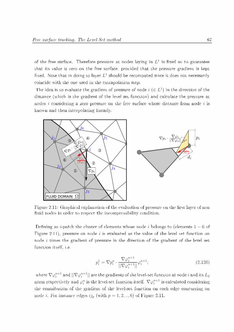
Free surfa e tra king. The Level Set method 67of the free surfa e. Therefore pressure at nodes laying in L1 is xed so to guaranteethat its value is zero on the free surfa e, provided that the pressure gradient is keptxed. Note that in doing so layer L1 should be re omputed sin e it does not ne essarily oin ide with the one used in the extrapolation step.The idea is to evaluate the gradient of pressure of node i (∈ L1) in the dire tion of thedistan e (whi h is the gradient of the level set fun tion) and al ulate the pressure atnodes i onsidering a zero pressure on the free surfa e whose distan e from node i isknown and then interpolating linearly.

FLUID DOMAIN

6

Figure 2.11: Graphi al explanation of the evaluation of pressure on the rst layer of nonuid nodes in order to respe t the in ompressibility ondition.Dening as i-pat h the luster of elements whose node i belongs to (elements 1 − 6 ofFigure 2.11), pressure on node i is evaluated as the value of the level set fun tion onnode i times the gradient of pressure in the dire tion of the gradient of the level setfun tion itself, i.e.p1i = ∇pni ·

∇ϕn+1i

||∇ϕn+1i ||ϕ

n+1i ; (2.126)where∇ϕn+1

i and ||∇ϕn+1i || are the gradients of the level-set fun tion at node i and its L2norm respe tively and ϕni is the level-set fun tion itself. ∇ϕn+1

i is al ulated onsideringthe ontribution of the gradient of the level-set fun tion on ea h edge on urring onnode i. For instan e edges ijp (with p = 1, 2, .., 6) of Figure 2.11.

68 The uid problemRemark 15. It is important to observe that Eqn.2.126 is the only point at whi h thelevel set fun tion is a tually required to be a distan e. Sin e its value is only needed onL1, it is onvenient to re ompute it as a urately as possible at every time step. This an be done geometri ally for the elements rossed by the zero of the level set fun tionwith a minor omputational ost.Remark 16. The orre t al ulation of the residual of the momentum equations wouldhave required integrating only on the uid area of the ut elements. This is impossiblewithin an edge-based formulation, unless one wants to re ompute the edges and losee ien y. In this work it is a epted to integrate on the whole element area onsideringthat both the body for e and the pressure gradient are extrapolated on the outside ofthe uid. This is a eptable for most situations and is exa t for the hydrostati asewhere the gradient of pressure and the body for e exa tly an el ea h other (see Se tion2.8.1 for an empiri al veri ation).2.7 The algorithmThe steps of the global algorithm are nally summarized in the box below.Element-based algorithm1. Given the level set fun tion ϕn, extrapolate velo ity, pressure and pressuregradient so to obtain un

ext, pnext and ∇pnext dened as the velo ity, pressure andpressure gradient over the extrapolated domain.2. Conve t the level set fun tion ϕ dening the new free surfa e at tn+1 using unand unext. Note that the extrapolated values are only required within a limitednumber of layers whi h are the ones on whi h the onve tion will be a tuallyperformed.3. Re- al ulate (if needed) the distan es in the whole domain starting from thezero of the level set fun tion at tn+1 obtained at step 2.4. Che k split elements and assemble only the uid sub-elements ontributions;5. Solve the monolithi system;6. Move to next time step.

The algorithm 69Edge-based algorithm1. Given the level set fun tion ϕn, extrapolate velo ity, pressure and pressuregradient so to obtain un

ext, pnext and ∇pnext dened as the velo ity, pressure andpressure gradient over the extrapolated domain.2. Conve t the level set fun tion ϕ dening the new free surfa e at tn+1 using unand unext. Note that the extrapolated values are only required within a limitednumber of layers whi h are the ones on whi h the onve tion will be a tuallyperformed.3. Re- ompute (if needed) the distan e in the whole domain starting from thezero of the level set fun tion at tn+1 obtained at step 2.4. Solve the momentum equations 2.91a. Note that the solution is performed onthe domain at the predi ted free surfa e position (ϕn+1).5. Set the approximate pressure boundary onditions on ∂Ωn+1 so to guaranteethat the pressure is (approximately) zero at the position indi ated by the zero ofthe level set fun tion. In order to do that, the geometri distan e is evaluated on

L1.6. Solve for the pressure (equation 2.91b).7. Solve for the orre tion (equation 2.91 ).8. Move to next time step.

70 The uid problem2.8 Numeri al examplesIn the following sub-se tions a series of ben hmark tests are presented. First two verysimple examples are presented to ompare the element-based and the edge-based freesurfa e algorithms for a variable porosity medium.Their performan e is analyzed both in the stati ase (Se tion 2.8.1) and in the dynami one (Se tion 2.8.2). In both ases the analyti al solution is known and is ompared withthe numeri al one obtained.The mass onservation apability is then analyzed both in a 2D and in a 3D example.No porous media is onsidered be ause its presen e has been veried to help mass onservation thanks to the introdu tion of an additional dissipative ee t.All the 3D examples are only performed with the edge-based algorithm being the onlyone implemented in 3D.In the last part of the se tion the edge-based te hnique for free surfa e ows (withoutporous medium) is tested in a series of examples and its results are ompared withresults obtained with a Lagrangian approa h using the Parti le Finite Element Method(PFEM).2.8.1 Still water exampleThe still water example allows to verify the orre t al ulation of pressure in a variableporosity medium.The domain of analysis is a square of 10m edge. The right hand side of the domain isporous (n = 0.5) whereas the left hand side is not (n = 1), as shown in Figure 2.12. Thelevel of water is set at y = 5m and slip boundary onditions are imposed on the bottomand on the side edges. Gravity is 10m/s2. Pressure is expe ted to vary linearly from0Pa at the free surfa e till 50000Pa at the bottom independently from whi h verti alse tion is hosen.The element-based algorithm reprodu es perfe tly the expe ted distribution. The dis-tribution of the iso-lines of pressure an be seen in Figure 2.13(a). No os illations areformed in the element-based example, onrming the exa t imposition of the pressureboundary ondition on the free surfa e via the element splitting te hnique des ribed inSe tion 2.6.4.For the edge-based algorithm, although the free surfa e does not move, a small os il-lation on the pressure is observed. This is aused by the approximated imposition of

Numeri al examples 71

Figure 2.12: Geometry, stru tured mesh and onditions of the still water model.

(a) Edge-based

(b) Element-basedFigure 2.13: Pressure distribution.

72 The uid problemthe zero pressure ondition on the free surfa e (see Se tion 2.6.4). The os illation of thebottom pressure is shown in Figure 2.13(a).

10000 0 10000 20000 30000 40000 50000PRESSURE [Pa]

0

2

4

6

8

10

Y [m

]

Element-BasedEdge-BasedAnalytical

Figure 2.14: Pressure distribution in a verti al se tion. Comparison between the twoalgorithms.Figure 2.14 nally shows the pressure distribution along a verti al se tion for bothalgorithms and it is ompared to the analyti al solution. The negative pressure of therst node above the free surfa e is the onsequen e of the imposition on the ut elementsof the zero pressure ondition on the free surfa e 2.6.4.2.8.2 Water owing through two materialsThe se ond example aims to analyze the behavior of the free surfa es algorithms whena variable porosity medium is present in dynami onditions. The domain of analysis isa square of edge 10m. Only the upper part is porous with porosity n = 0.5 while thelower part orresponds to a pure air material (n = 1). A verti al entran e of water isset from the bottom edge. Slip boundary onditions are imposed to the verti al walls

Numeri al examples 73

Figure 2.15: Geometry, stru tured mesh and onditions of the two material model withbottom in oming water.and 0Pa pressure ondition is set, in the ase of the edge-based algorithm, to the upperside. The mesh is stru tured as shown in Figure 2.15.In the sequen es presented in Figure 2.16 the free surfa e line is perturbed when enteringthe porous media. Nevertheless it re overs the horizontal plane shape as soon as thedis ontinuity has passed.Figures 2.17 and 2.18 show the distribution of pressure in the verti al entral se tion ofthe two models, when the water level is 2.5m and 9.9m respe tively. A omparison withthe analyti al results is presented. There is a very good a ordan e of pressure valuesin the ase that no porous media is still present, as an be seen in Figure 2.17. Theelement-based algorithm perfe tly al ulate the pressure distribution also when waterhas entered the porous media. On the ontrary the error of the edge-based algorithm isnot negligible (Figure 2.18).

74 The uid problem

(a) Edge-based. (b) Element-based.Figure 2.16: Evolution of free surfa e for both algorithms.

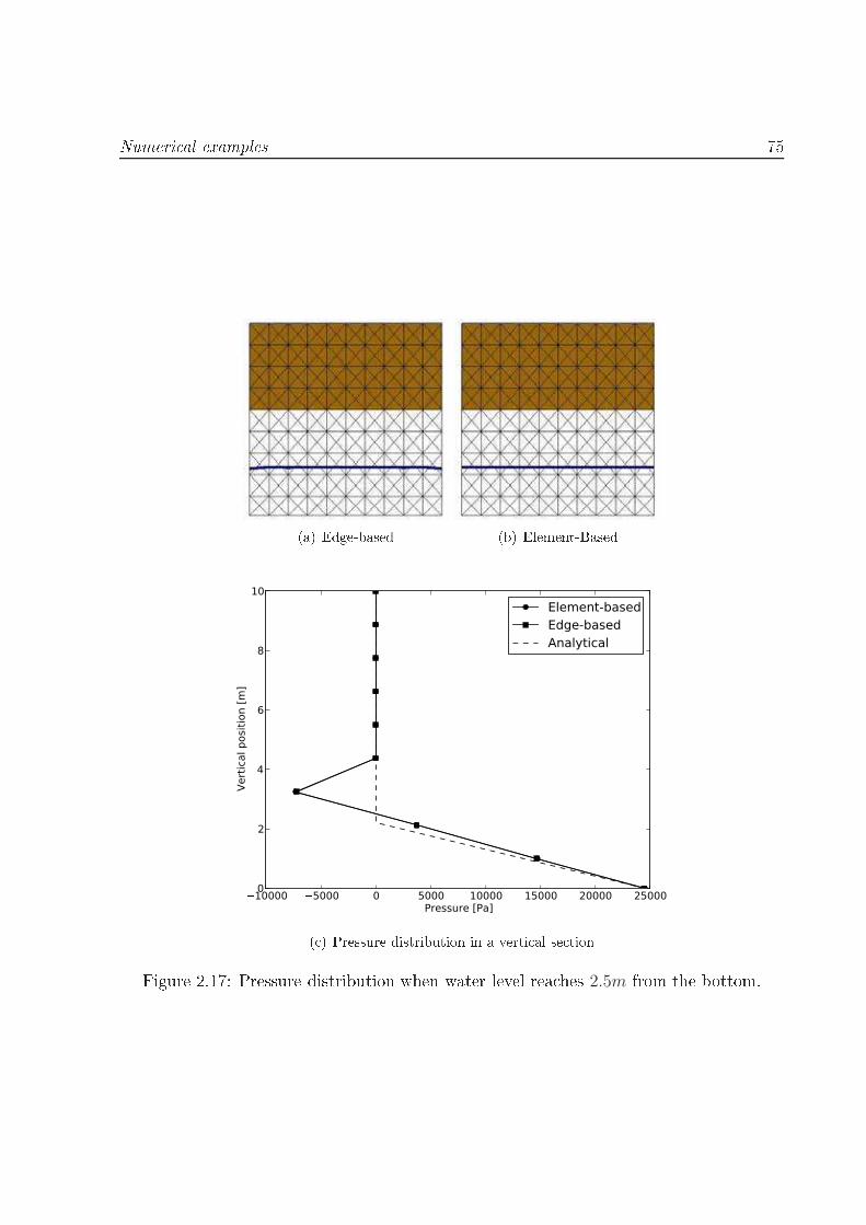
Numeri al examples 75

(a) Edge-based (b) Element-Based

100005000 0 5000 10000 15000 20000 25000Pressure [Pa]

0

2

4

6

8

10

Vert

ical

pos

ition

[m]

Element-basedEdge-basedAnalytical

( ) Pressure distribution in a verti al se tionFigure 2.17: Pressure distribution when water level rea hes 2.5m from the bottom.

76 The uid problem

(a) Edge-based (b) Element-Based

0 500000 1000000 1500000 2000000 2500000 3000000 3500000 4000000Pressure [Pa]

0

2

4

6

8

10

Vert

ical

pos

ition

[m]

Element-basedEdge-basedAnalytical

( ) Pressure distribution in a verti al se tionFigure 2.18: Pressure distribution when water level rea hes the top.

Numeri al examples 772.8.3 Mass onservation2D verti al olumn Edge-based and element-based methodA se ond example has been performed in order to he k the mass onservation apabilityin both algorithms. No porous media has been onsidered (n = 1) be ause its dissipativeee t has been shown to help the mass to be onserved. The worst ase is then analyzed.A re tangular domain of 5m width and 10m height is set. A dis harge of 1m3/s isentering the domain from the bottom edge. The inlet verti al velo ity is then 0.2m/s.Slip boundary onditions are imposed on the verti al edges and zero pressure is imposedon the upper edge (only for the edge-based formulation).Two dierent meshes are onsidered as shown in Fig.2.19.

INCOMING WATER vy= 0.2m/s

SL

IP C

ON

DIT

ION

SLIP

CO

ND

ITIO

N

10m

5m

(a) Mesh 0.2 m (b) Mesh 0.5 mFigure 2.19: Geometry, mesh and onditions of the mass onservation model.A good onservation of mass is seen in both algorithms. Figures 2.20 and 2.21 showthe evolution of the free surfa e at 10− 20− 30− 40− 50 sec respe tively.3D Verti al olumn edge-based methodIn the present example a verti al re tangular olumn with an inlet in the bottom sideand an outlet on the top fa e is simulated. Geometry and onditions of the present

78 The uid problem

(a) Mesh 0.2 m

(b) Mesh 0.5 mFigure 2.20: 2D Verti al olumn. Element-based algorithm. Evolution of free surfa eat 10− 20− 30− 40− 50 sec.

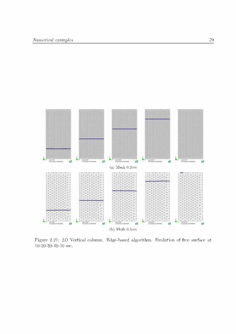
Numeri al examples 79

(a) Mesh 0.2cm

(b) Mesh 0.5cmFigure 2.21: 2D Verti al olumn. Edge-based algorithm. Evolution of free surfa e at10-20-30-40-50 se .

80 The uid problemexample are taken from [43 (although in that ase the intera tion between two uidswith dierent spe i weight was taken into a ount). Nevertheless the problem presentsthe same di ulties of maintenan e of a at free surfa e both in the transitory and inthe stationary regime.The problem has been studied using two meshes: a stru tured one and an unstru turedone (Figure 2.22). STRUCTURED UNSTRUCTUREDMedium Medium Coarsen. nodes. 2981 1210 723n. elem 13800 6117 3720elem length [m - 1 1.2elem per side 5× 5× 20 - -Table 2.6: 3D verti al olumn. Number of nodes, number of elements, elemental length(unstru tured meshes) and number of elements per edge (stru tured mesh) of the meshes onsidered in the analysis.Figures 2.23 and 2.24 show the evolution of the free surfa e (identied with the zeroof the level set fun tion (ϕ = 0) during the lling pro ess. Considering that the freesurfa e at time t = 0 is lo ated at h = 1m from the bottom and the velo ity inlet isv = 1m/s a very good agreement with expe ted level of the free surfa e an be noti edat ea h time step (Figures 2.23 and 2.24). In both ases the expe ted level of water at2s, 6s, 10s, 14s and 18s is respe ted and it is 3m, 7m, 11m, 15m and 19m respe tively.No os illations are observed neither for the unstru tured nor the stru tured mesh.If a lateral entran e of water is onsidered and the value of inlet velo ity is de reasedto vin = 0.1m/s (see Figure 2.25 for the details on the geometry and the boundary onditions onsidered), the improvement of volume onservation explained in Se tion2.5.5 plays a relevant role. Two meshes are onsidered for the al ulation: a oarse anda ne one whose hara teristi s are summarized in Table 2.7 and shown in Figure 2.27.Figure 2.26(a) shows the bene ial ee t of the volume orre tion. The expe ted levelof water is ompared with the one al ulated for the ne mesh model with and withoutvolume onservation improvements. On the other hand, it is important to observe that

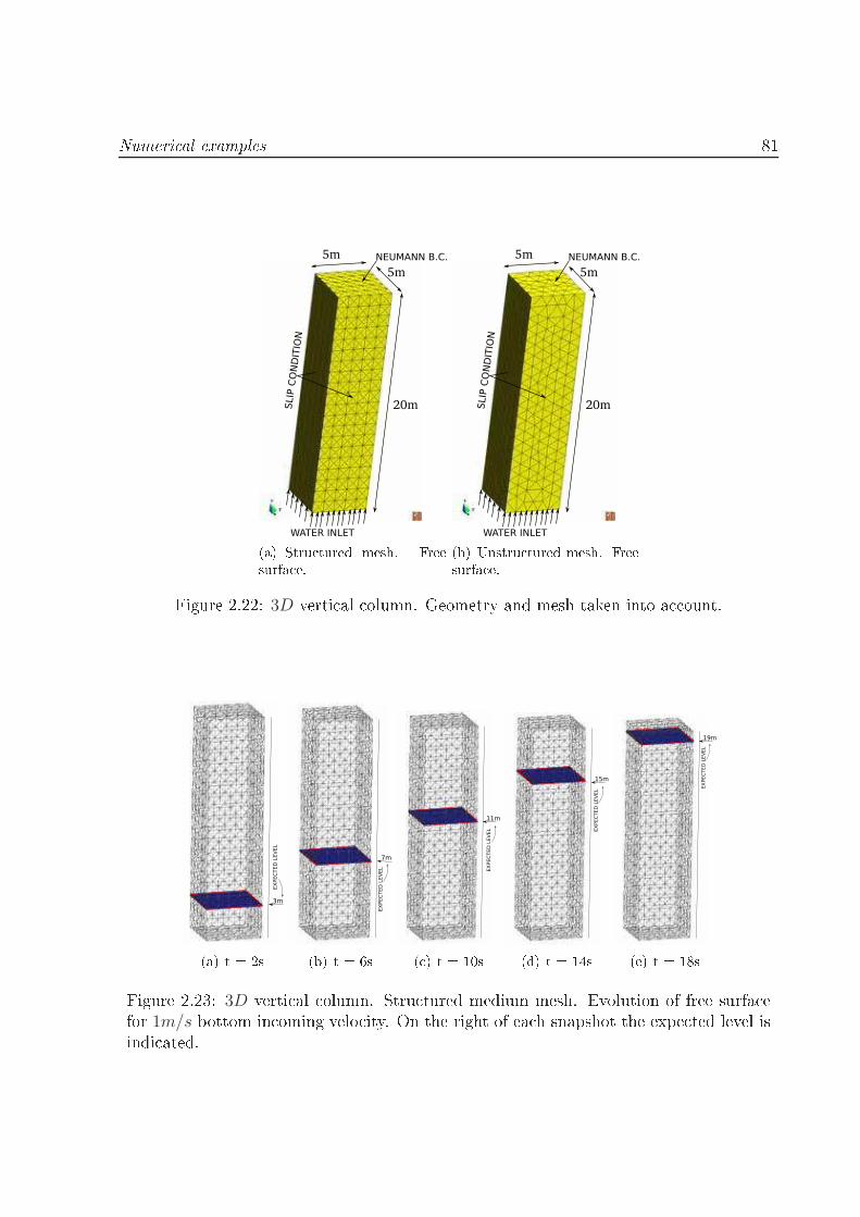
Numeri al examples 81

20mSLIP

CO

ND

ITIO

N

NEUMANN B.C.

5m

5m

WATER INLET(a) Stru tured mesh. Freesurfa e.20mS

LIP

CO

ND

ITIO

N

NEUMANN B.C.

5m

5m

WATER INLET(b) Unstru tured mesh. Freesurfa e.Figure 2.22: 3D verti al olumn. Geometry and mesh taken into a ount.

3m

EX

PEC

TED

LEV

EL

(a) t = 2s7m

EX

PEC

TED

LEV

EL

(b) t = 6s11m

EX

PEC

TED

LEV

EL

( ) t = 10s15m

EX

PEC

TED

LEV

EL

(d) t = 14s

19m

EX

PEC

TED

LEV

EL

(e) t = 18sFigure 2.23: 3D verti al olumn. Stru tured medium mesh. Evolution of free surfa efor 1m/s bottom in oming velo ity. On the right of ea h snapshot the expe ted level isindi ated.

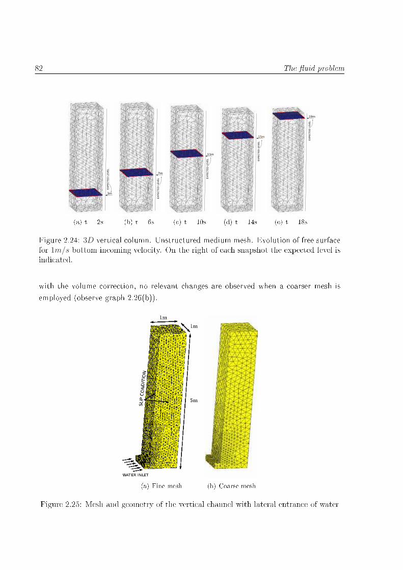
82 The uid problem

3m

EX

PEC

TED

LEV

EL

(a) t = 2s7m

EX

PEC

TED

LEV

EL

(b) t = 6s11m

EX

PEC

TED

LEV

EL

( ) t = 10s15m

EX

PEC

TED

LEV

EL

(d) t = 14s

19m

EX

PEC

TED

LEV

EL

(e) t = 18sFigure 2.24: 3D verti al olumn. Unstru tured medium mesh. Evolution of free surfa efor 1m/s bottom in oming velo ity. On the right of ea h snapshot the expe ted level isindi ated.with the volume orre tion, no relevant hanges are observed when a oarser mesh isemployed (observe graph 2.26(b)).

(a) Fine mesh (b) Coarse meshFigure 2.25: Mesh and geometry of the verti al hannel with lateral entran e of water

Numeri al examples 83Another important aspe t is that the use of the volume orre tion leads to a at freesurfa e redu ing the os illations. This an be observed by omparing Figures 2.27(a)and 2.27(b) where the volume orre tion is used in both the ne and oarse mesh withFigures 2.27( ) where not. Fine Coarsen. nodes. 12 100 3 050n. elem 61 600 14 400Table 2.7: Verti al olumn with lateral entran e example. Number of nodes and numberof elements for the meshes onsidered in the analysis.

0 50 100 150 200TIME [s]

0

1

2

3

4

5

WAT

ER H

EIG

HT [P

a]

EXACT SOLUTIONFINE WITHOUT VOLUME CORRECTIONFINE WITH VOLUME CORRECTION

(a) With or without volume orre tion. Finemesh. 0 50 100 150 200TIME [s]

0

1

2

3

4

5

WAT

ER H

EIG

HT [P

a]

EXACT SOLUTIONFINE WITH VOLUME CORRECTIONCOARSE WITH VOLUME CORRECTION

(b) With volume orre tion. Coarse and nemesh.Figure 2.26: Verti al olumn with lateral entran e example. Level of water in terms oftime.

84 The uid problem

(a) With volume orre tion. Fine mesh model

(b) With volume orre tion. Coarse mesh model

( ) Without volume orre tion. Fine mesh modelFigure 2.27: Verti al olumn with lateral entran e example. Evolution of the free surfa eat 50s, 120s, and 230s.

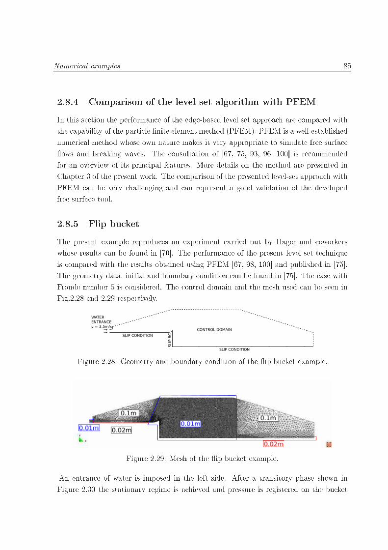
Numeri al examples 852.8.4 Comparison of the level set algorithm with PFEMIn this se tion the performan e of the edge-based level set approa h are ompared withthe apability of the parti le nite element method (PFEM). PFEM is a well establishednumeri al method whose own nature makes it very appropriate to simulate free surfa eows and breaking waves. The onsultation of [67, 75, 93, 96, 100 is re ommendedfor an overview of its prin ipal features. More details on the method are presented inChapter 3 of the present work. The omparison of the presented level-set approa h withPFEM an be very hallenging and an represent a good validation of the developedfree surfa e tool.2.8.5 Flip bu ketThe present example reprodu es an experiment arried out by Hager and oworkerswhose results an be found in [70. The performan e of the present level set te hniqueis ompared with the results obtained using PFEM [67, 98, 100 and published in [75.The geometry data, initial and boundary ondition an be found in [75. The ase withFroude number 5 is onsidered. The ontrol domain and the mesh used an be seen inFig.2.28 and 2.29 respe tively.SLIP CONDITION

SLIP CONDITION

SLIP

BC

WATER

ENTRANCE

v = 3.5m/sCONTROL DOMAINFigure 2.28: Geometry and boundary ondition of the ip bu ket example.

Figure 2.29: Mesh of the ip bu ket example.An entran e of water is imposed in the left side. After a transitory phase shown inFigure 2.30 the stationary regime is a hieved and pressure is registered on the bu ket

86 The uid problem

Figure 2.30: Sequen e of the transitory phase of the jet.as shown in Figure 2.31(a). The jet shape is also ompared in Figure 2.31(b) where thedarker line is the level set whereas the lighter represents the PFEM results.A good agreement with experimental pressure along the bu ket an be seen in Fig-ure 2.31(a). The bla k points are the experimental results found in [70, whereas the ontinuous line and the dotted line are the level set and the PFEM solutions respe tively.2.8.6 3D dambreakThe present example is a 3D dam break example already studied by the authors in [75using PFEM.Data are taken from the experiments performed at the Maritime Resear h InstituteNetherlands (MARIN) for breaking dam ows [72. Several numeri al results of this asestudy are available in literature for VOF te hniques. This is the ase of [72 employingCartesian grids, or [54 using an edge-based approa h. Finally other level set simulations an also be found. Among others, in [7, 71, an appli ation of isogeometri analysis ispresented.The water olumn is left free to fall over a step where pressure sensors are set following

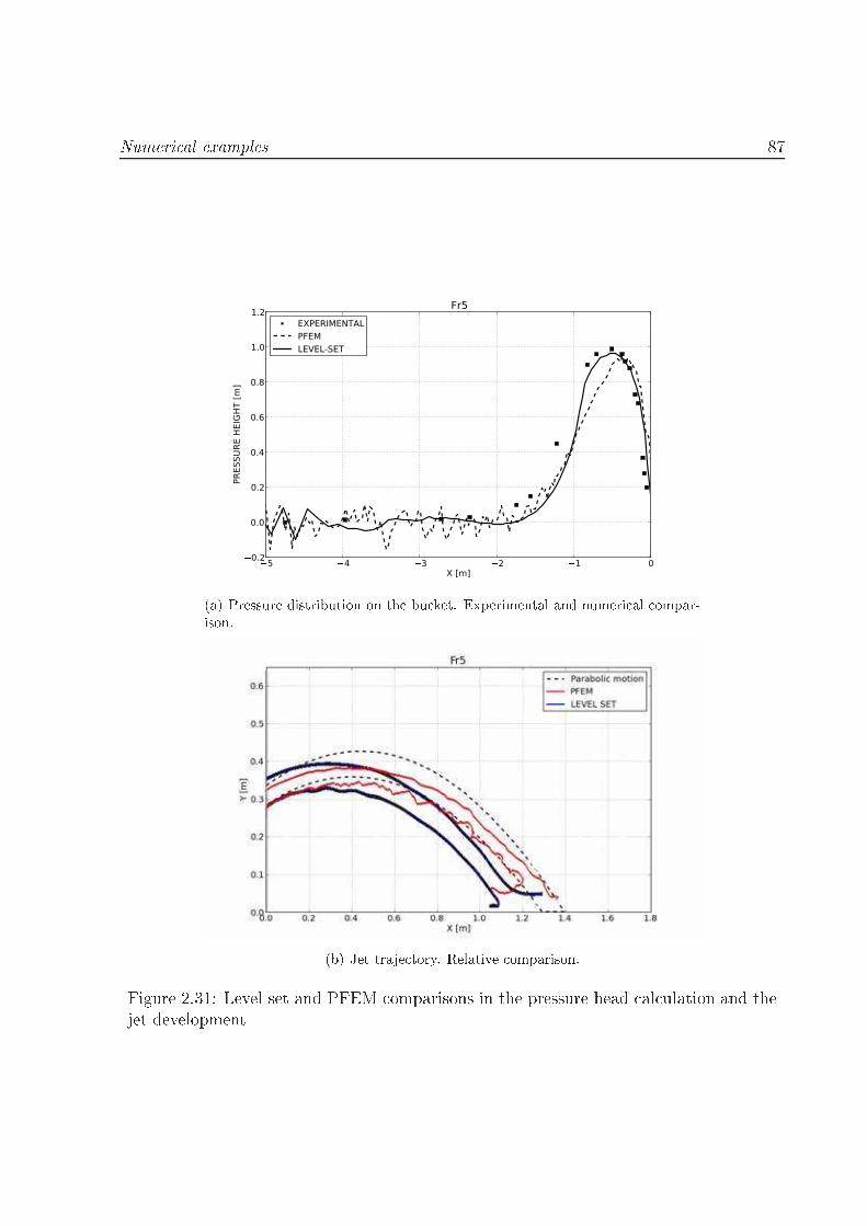
Numeri al examples 87

5 4 3 2 1 0X [m]

0.2

0.0

0.2

0.4

0.6

0.8

1.0

1.2

PRES

SURE

HEI

GHT

[m]

Fr5EXPERIMENTALPFEMLEVEL-SET

(a) Pressure distribution on the bu ket. Experimental and numeri al ompar-ison.

(b) Jet traje tory. Relative omparison.Figure 2.31: Level set and PFEM omparisons in the pressure head al ulation and thejet development

88 The uid problemthe s heme of Figure 2.32. The details of geometry an be found in [54.WATER

STEP WITH PRESSURE SENSORS

SLIP CONDITION ON THE WALLS

1.22m

0.5

5m

0.4

5m

2.00m

0.8245m

IMPACT DIR

0.1

61m

0.403m

0.021m

0.04m

0.04m

0.04m

P1

P2

P3

P4

P5P6

P7P8

0.021m0.04m

0.04m0.04m

0.161m

IMPACT D

IR

Figure 2.32: Geometry and boundary ondition of the 3D dam break example. On thelower left orner a zoom on the pressure sensors distribution on the stepTwo meshes are onsidered in the present work, their hara teristi s are detailed inTable2.8 and they are shown in Figure2.33.Mesh A Mesh Bn. nodes. 51 627 392 130n. elem 296 157 2 310 984Table 2.8: Dam break example. Number of nodes and number of elements of the twomeshes onsidered in the analysis.A sequen e of the falling of the water olumn an be seen in Figure 2.34 where the freesurfa e evolution is plotted for the two meshes onsidered.

Numeri al examples 89

(a) Mesh A. (b) Mesh B.Figure 2.33: The two meshes onsidered. On the left Mesh A of 296 157 and Mesh B of2 310 984 tetrahedra.

(a) Mesh A. (b) Mesh B.Figure 2.34: Evolution of the dam break at 0.4s, 0.6s and 2.0s. Comparison betweenthe results obtained with meshes A and B.

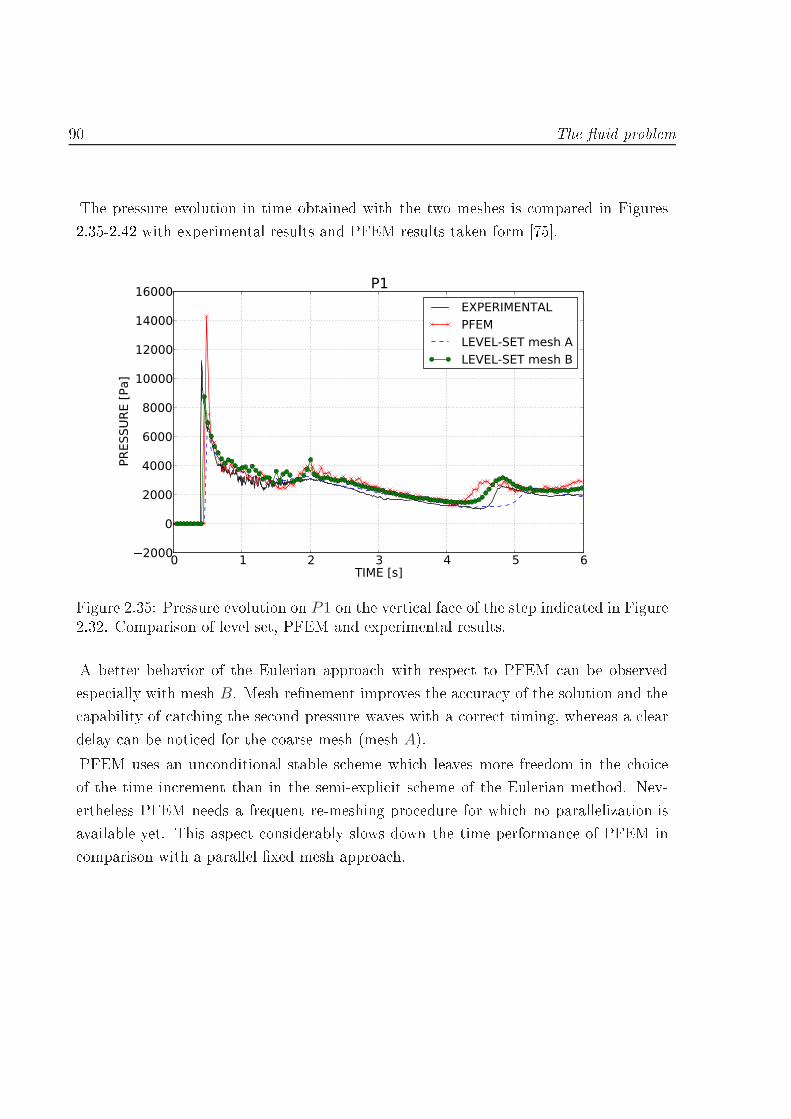
90 The uid problemThe pressure evolution in time obtained with the two meshes is ompared in Figures2.35-2.42 with experimental results and PFEM results taken form [75.

0 1 2 3 4 5 6TIME [s]

2000

0

2000

4000

6000

8000

10000

12000

14000

16000

PRES

SURE

[Pa]

P1EXPERIMENTALPFEMLEVEL-SET mesh ALEVEL-SET mesh B

Figure 2.35: Pressure evolution on P1 on the verti al fa e of the step indi ated in Figure2.32. Comparison of level set, PFEM and experimental results.A better behavior of the Eulerian approa h with respe t to PFEM an be observedespe ially with mesh B. Mesh renement improves the a ura y of the solution and the apability of at hing the se ond pressure waves with a orre t timing, whereas a leardelay an be noti ed for the oarse mesh (mesh A).PFEM uses an un onditional stable s heme whi h leaves more freedom in the hoi eof the time in rement than in the semi-expli it s heme of the Eulerian method. Nev-ertheless PFEM needs a frequent re-meshing pro edure for whi h no parallelization isavailable yet. This aspe t onsiderably slows down the time performan e of PFEM in omparison with a parallel xed mesh approa h.

Numeri al examples 91

0 1 2 3 4 5 6TIME [s]

2000

0

2000

4000

6000

8000

10000

12000

14000

16000

PRES

SURE

[Pa]

P2EXPERIMENTALPFEMLEVEL-SET mesh ALEVEL-SET mesh B

Figure 2.36: Pressure evolution on P2 on the verti al fa e of the step indi ated in Fig.2.32. Comparison of level set, PFEM and experimental results.

0 1 2 3 4 5 6TIME [s]

2000

0

2000

4000

6000

8000

10000

12000

14000

16000

PRES

SURE

[Pa]

P3EXPERIMENTALPFEMLEVEL-SET mesh ALEVEL-SET mesh B

Figure 2.37: Pressure evolution on P3 on the verti al fa e of the step indi ated in Fig.2.32. Comparison of level set, PFEM and experimental results.

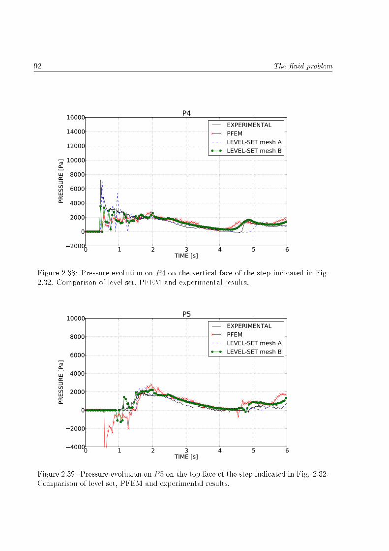
92 The uid problem

0 1 2 3 4 5 6TIME [s]

2000

0

2000

4000

6000

8000

10000

12000

14000

16000

PRES

SURE

[Pa]

P4EXPERIMENTALPFEMLEVEL-SET mesh ALEVEL-SET mesh B

Figure 2.38: Pressure evolution on P4 on the verti al fa e of the step indi ated in Fig.2.32. Comparison of level set, PFEM and experimental results.

0 1 2 3 4 5 6TIME [s]

4000

2000

0

2000

4000

6000

8000

10000

PRES

SURE

[Pa]

P5EXPERIMENTALPFEMLEVEL-SET mesh ALEVEL-SET mesh B

Figure 2.39: Pressure evolution on P5 on the top fa e of the step indi ated in Fig. 2.32.Comparison of level set, PFEM and experimental results.

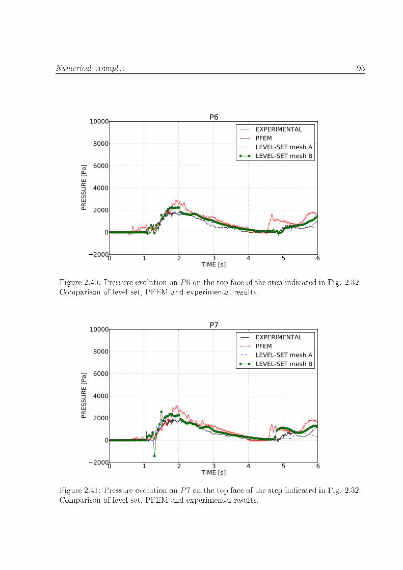
Numeri al examples 93

0 1 2 3 4 5 6TIME [s]

2000

0

2000

4000

6000

8000

10000

PRES

SURE

[Pa]

P6EXPERIMENTALPFEMLEVEL-SET mesh ALEVEL-SET mesh B

Figure 2.40: Pressure evolution on P6 on the top fa e of the step indi ated in Fig. 2.32.Comparison of level set, PFEM and experimental results.

0 1 2 3 4 5 6TIME [s]

2000

0

2000

4000

6000

8000

10000

PRES

SURE

[Pa]

P7EXPERIMENTALPFEMLEVEL-SET mesh ALEVEL-SET mesh B

Figure 2.41: Pressure evolution on P7 on the top fa e of the step indi ated in Fig. 2.32.Comparison of level set, PFEM and experimental results.

94 The uid problem

0 1 2 3 4 5 6TIME [s]

2000

0

2000

4000

6000

8000

10000

PRES

SURE

[Pa]

P8EXPERIMENTALPFEMLEVEL-SET mesh ALEVEL-SET mesh B

Figure 2.42: Pressure evolution on P8 on the top fa e of the step indi ated in Fig. 2.32.Comparison of level set, PFEM and experimental results.2.9 Con lusionsIn this hapter the approa h to numeri ally treat the problem of ow in a variableporosity medium has been presented. After the hoi e of the resistan e law to be usedin the algorithm, the two solution methods developed have been presented in detail:• Element-based algorithm. It uses a monolithi approa h to solve the weak formof the balan e equations that are stabilized using an ASGS te hnique. A fullyimpli it method is used and a Bossak time integration te hnique is hosen.• Edge-based algorithm. In this ase a fra tional step approa h is used to solvethe balan e equations that are stabilized using an OSS stabilization te hnique. Asemi-expli it method, i.e. a 4th order Runge Kutta s heme is implemented.In both ases only simpli ial meshes (3-noded triangles or 4-noded tethraedra) are takeninto a ount.The dynami free surfa e tra king is done using a level set te hnique des ribed in these ond part of the hapter. An expli it extrapolation is performed in order to denethe values of velo ity on a band ontaining the free surfa e of the uid. The level

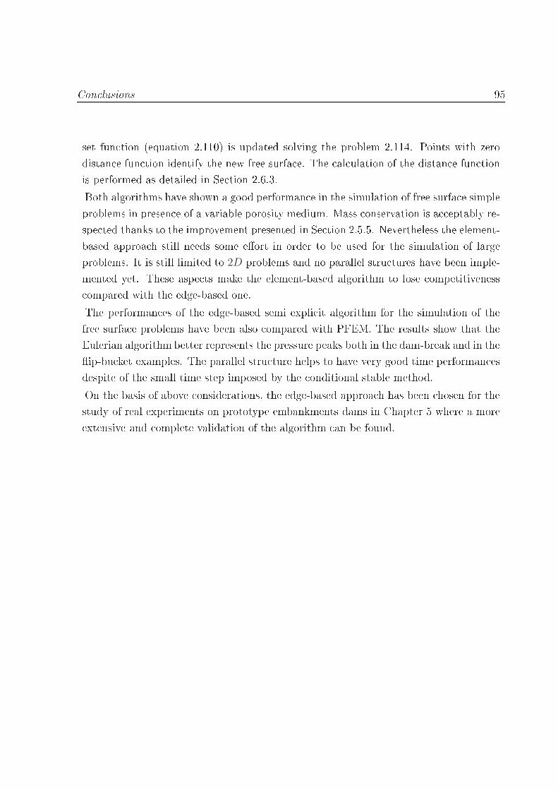
Con lusions 95set fun tion (equation 2.110) is updated solving the problem 2.114. Points with zerodistan e fun tion identify the new free surfa e. The al ulation of the distan e fun tionis performed as detailed in Se tion 2.6.3.Both algorithms have shown a good performan e in the simulation of free surfa e simpleproblems in presen e of a variable porosity medium. Mass onservation is a eptably re-spe ted thanks to the improvement presented in Se tion 2.5.5. Nevertheless the element-based approa h still needs some eort in order to be used for the simulation of largeproblems. It is still limited to 2D problems and no parallel stru tures have been imple-mented yet. These aspe ts make the element-based algorithm to lose ompetitiveness ompared with the edge-based one.The performan es of the edge-based semi expli it algorithm for the simulation of thefree surfa e problems have been also ompared with PFEM. The results show that theEulerian algorithm better represents the pressure peaks both in the dam-break and in theip-bu ket examples. The parallel stru ture helps to have very good time performan esdespite of the small time step imposed by the onditional stable method.On the basis of above onsiderations, the edge-based approa h has been hosen for thestudy of real experiments on prototype embankments dams in Chapter 5 where a moreextensive and omplete validation of the algorithm an be found.

Chapter 3The stru tural problemIn this hapter an algorithm to simulate the behavior of the granular non- ohesivematerial used in ro kll dams is proposed. Taking into a ount the high deformationthe stru ture might be subje ted to and the intrinsi in oheren e of the ro ks, the onstitutive law of a non-Newtonian high vis osity material is hosen. After an overviewof the traditional non-Newtonian relationships, a regularized Bingham model is sele tedand implemented as a starting point. This approa h presents severe limitations in thesimulation of granular behavior having a onstant yield threshold. To over ome thisissue a variable yield model using a Mohr Coulomb failure riteria is proposed in these ond part of the hapter.The weak form of the problem is then obtained and the numeri al te hnique adoptedis presented. The Lagrangian Parti le Finite Element Method (PFEM) is hosen for itswide exibility. In fa t the stru tural domain is expe ted to undergo severe deformationsas the failure progresses and therefore a Lagrangian approa h is a natural hoi e.In the last part of the hapter the validation of the Binghammodel is performed throughsome ben hmarks and the ee tiveness of the proposed variable yield model is tested insome examples.3.1 Introdu tionIn the present work, the simulation of the stru tural response of a slope made of granularmaterial has been fa ed using a ontinuous approa h despite the intrinsi in oherentnature of the ro kll. This is an a eptable hoi e under the assumption that the

98 The stru tural problemro kll size is small with respe t to the overall size of the stru ture.Nevertheless it should be mentioned that in re ent years, the great advan e in omputerperforman e and in parallel omputing has allowed the simulation of the me hani albehaviour of every single parti le of a granular slope. The family of the so alled dis rete(or distin t) element methods (DEM) has been rea hing a widespread popularity in the omputational me hani s ommunity. Their basi idea is that every parti le is a dis reteelement intera ting with the others onsidering its me hani al and material properties.This an be a valid alternative to the model presented in this hapter and it is a tuallybeing implemented by other resear hers at CIMNE.The adoption of a ontinuous approa h leads to an additional requirement: the hoi eof a suitable onstitutive law. Many plasti or rigid-plasti onstitutive models are ommonly used in geome hani s to des ribe the stru tural response of an in oherentnon- ohesive material. It is usually a epted that a ro kll slope has the apability tosupport a ertain amount of shear stress with almost no elasti strains before startinglarge deformations. When the yield stress is rea hed the material starts to ow untilarriving to a stable onguration. It should be noted that the behaviour of the yieldedmaterial is more similar to the owing of a uid than to the pro ess of deformation ofa solid. On the other hand, in literature there exists a wide ategory of uids whi hexhibits a rigid behaviour till rea hing a yield threshold. They are part of the family ofthe so alled non-Newtonian uids.These aspe ts, together with the natural way of managing large deformations in uids,lead us to on entrate on variable vis osity models for the al ulation of the stru turalpart instead than on any other plasti or damage model. Consequently, a non-Newtonian onstitutive law has been adopted for the ro kll body. This implies that the ro kllstiness is ontrolled by very high values of the vis osity. Only when the yield thresholdis ex eeded, the vis osity dramati ally de reases and the material starts owing. Whenthe material stops its motion, the vis osity re overs its initial values for whi h the stresslevel does not ex eed the yield limit.The model developed in this work has its origin in the traditional Bingham plasti susing the regularization proposed by Papanastasiou to over ome numeri al problemsindu ed by the bilinear stress-strain urve [104. Nevertheless in order to in lude a Mohr-Coulomb failure riteria (without ohesion), the possibility of onsidering a variable yieldlevel is introdu ed.The two onstitutive models with onstant and variable yield, are presented at the

Stru tural onstitutive law. An overview of non-Newtonian models 99beginning of the present hapter after a brief overview on non-Newtonian models.The equations governing the stru tural problem are studied in their weak form arrivingto the algebrai solution system whi h is solved with a fully impli it approa h. A stabi-lized, equal-order, mixed velo ity-pressure element te hnology is hosen so to guaranteea lo king free behavior. In fa t Cervera and oworkers have demonstrated that the use ofa mixed approa h is the appropriate framework for dealing with lo alization problems inin ompressible and quasi-in ompressible problems. They have su essfully applied thisapproa h in solid me hani s in plasti and damage models using linear/linear elements,providing a suitable stabilization te hnique [2529, 32.Sin e the stru tural domain is expe ted to undergo severe deformations as the failureprogresses, the kinemati model has to adapt dynami ally to su h deformations. TheParti le Finite Element Method (PFEM) provides the ne essary exibility with a pow-erful remeshing me hanism [75, 100. Its features are des ribed in the se ond part ofthis hapter.In the last part of the hapter some examples are inserted to validate the Binghammodel and to appre iate its dieren es with respe t to the proposed variable vis osityapproa h. Finally some dambreaks of granular slopes with dierent fri tional anglesare simulated to verify that the model orre tly reprodu es the expe ted me hani alproperties.3.2 Stru tural onstitutive law. An overview of non-Newtonian modelsIn Chapter 2 the onstitutive model of a Newtonian uid was used to des ribe the stress-strain behavior of water. The stress tensor an be de omposed in its hydrostati anddeviatori parts as followσ = −pI + τ = −pI + 2µε(u), (3.1)where

ε(u) := ∇su =1

2

(

∇u+ (∇u)T)

, (3.2)The deviatori part of the stress tensor τ , is therefore linearly related to the rate ofstrain ε(u) through the onstant vis osity µ.

100 The stru tural problemFluids for whi h the relations between τ and ε(u) is not onstant, are alled non-Newtonians. In this ase vis osity annot be onsidered as a property of the materialas it is stri tly dependent on the deformation pro ess. This lassi ation is very generaland in ludes a wide range of dierent onstitutive relations. In order to briey lassifythe dierent non-Newtonian uids, let's onsider the 1d problem and let's dene anapparent vis osity µ like the ratio between the shear stress τ and the shear rate γ

µ := µ(γ) =τ

γ. (3.3)A ording to Chhabra [31 a possible lassi ation of the non-Newtonian uids is thefollowing:- Fluids with time independent behavior: those for whi h the urrent shear stressis fun tion only of the shear rate τ = τ(γ). In fun tion of the evolution of theirapparent vis osity, they an be divided in:1. Shear-thinning or pseudo-plasti uids. Their apparent vis osity gradu-ally de reases when in reasing the shear rate. This is the ase of polymeri systems like melts and solutions.2. Shear-thi kening or dilatant uids. Their apparent vis osity in reases whenthe shear rates in reases. This behavior is observed in on entrated suspen-sions, for instan e.3. Vis o-plasti uids (with or without shear thinning behavior). They are hara terized by the existen e of a threshold stress, the yield stress, whi hmust be ex eeded for the uid to deform. For lower values of stress the vis o-plasti uids are ompletely rigid or an show some sort of elasti ity. On ethe yield stress is rea hed and ex eeded, they an exhibit a Newtonian-likebehavior with a onstant apparent vis osity (Bingham plasti s uids) or not,showing a shear thinning behavior (yield-pseudoplasti uids).- Fluids with time dependent behavior: their apparent vis osity is not only afun tion of shear stress and shear rate but also of the duration of the appli ationof the shear stress and of its kinemati history. They an be lassied into:1. Thixotropi . Under a onstant shear their apparent vis osity de reases withtime. A typi al thixotropi material is the ement paste.

Stru tural onstitutive law. An overview of non-Newtonian models 1012. Rheope ti . Under onstant shearing their apparent vis osity in reases withtime. For instan e printers inks belong to this group.A s hemati overview of the relation between shear stress and rate of strain for dierentnon-Newtonian models an be observed in Figure 3.1.NEWTONIAN

DILATANT

PSEUDOPLASTIC

VISCOPLASTIC

BINGHAM

SHEAR RATE

SH

EA

R S

TR

ESS

Figure 3.1: Qualitative ow urves for the dierent ategories of non-Newtonian uids.A deep analysis of non-Newtonian uids behavior falls outside the s ope of this work.For a omprehensive review of the topi see [24, 31, 44.3.2.1 Constant yield: the Bingham modelIt was in 1919 when Eugene C. Bingham, while studying a possible onstitutive modelfor paints, dis overed that their deformation was almost absent till rea hing a threshold:the yield stress. After ex eeding this stress limit they followed a Newtonian behavior.A ording to Papanastasiou [104 a wide range of materials have been identied to havea yield threshold. Bird [15 was the rst to give, in his book, a lists of several Binghamplasti s, most of these produ ts ame from food or hemi al industry. Among them we an list for instan e slurries, pastes, nails, or food substan es like margarine, ket hup,mayonnaise and others.The 1D onstitutive relation for a Bingham plasti an be dened as follows. Being τ0

102 The stru tural problemthe yield stressγ = 0 if τ < τ0

γ =1

µs(τ − τ0) if τ ≥ τ0

(3.4)where γ is the rate of strain, µ is the dynami vis osity and τ the shear stress.Figure 3.2 shows the dieren e between a Newtonian and a Non Newtonian uid.

RATE OF STRAIN

SHE

AR S

TRES

S0Bingham plasticNewtonian fluid

Figure 3.2: Comparison between a Newtonian uid and a Bingham uid behavior witha yield stress τ0.Equation 3.4 an be rewritten asτ =

(

µs +τ0γ

)

γ if τ ≥ τ0. (3.5)Spe ial are should be taken in equation 3.5 when the level of stress is lower than theyield stress. In this ase, a ording to equation 3.3, the apparent vis osity approa hesinnity, i.e. µ → ∞ as γ → 0. This behavior might indu e numeri al di ulties, somesmooth laws are usually preferred. Nevertheless some authors [80 tried to simulate whatis alled bi-vis osity model but their predi tions leads to in onsisten ies. Consequently,in the present work the regularized model proposed by Papanastasiou [104 is hosen asa starting point for the development.Following the ideas presented in [104, equation 3.4 is regularized as follow

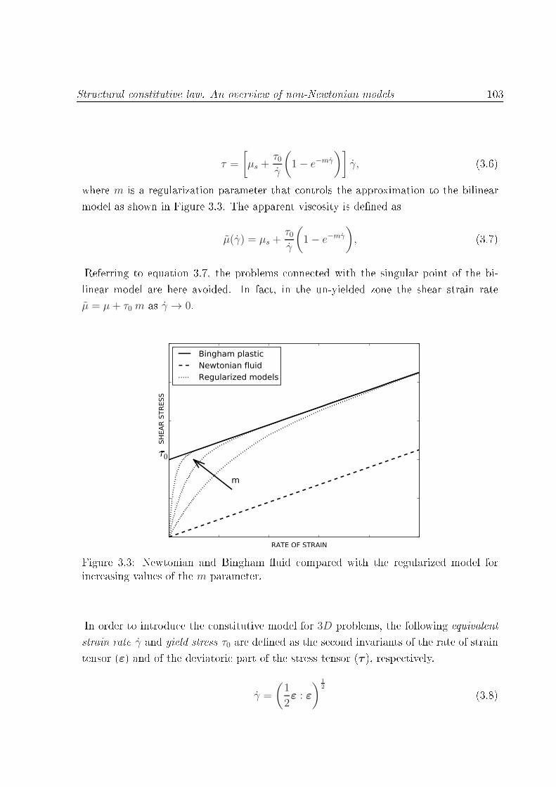
Stru tural onstitutive law. An overview of non-Newtonian models 103τ =

[

µs +τ0γ

(

1− e−mγ

)]

γ, (3.6)where m is a regularization parameter that ontrols the approximation to the bilinearmodel as shown in Figure 3.3. The apparent vis osity is dened asµ(γ) = µs +

τ0γ

(

1− e−mγ

)

, (3.7)Referring to equation 3.7, the problems onne ted with the singular point of the bi-linear model are here avoided. In fa t, in the un-yielded zone the shear strain rateµ = µ+ τ0 m as γ → 0.

RATE OF STRAIN

SHE

AR S

TRES

S

m

0Bingham plasticNewtonian fluidRegularized models

Figure 3.3: Newtonian and Bingham uid ompared with the regularized model forin reasing values of the m parameter.In order to introdu e the onstitutive model for 3D problems, the following equivalentstrain rate γ and yield stress τ0 are dened as the se ond invariants of the rate of straintensor (ε) and of the deviatori part of the stress tensor (τ ), respe tively.γ =

(1

2ε : ε

) 1

2 (3.8)

104 The stru tural problemτ0 =

(1

2τ : τ

) 1

2 (3.9)Equation 3.6 be omes for 3D problems asτ = 2

[

µs +τ0γ

(

1− e−mγ

)]

ε(u), (3.10)whereµ(γ) = µs +

τ0γ

(

1− e−mγ

)

, (3.11)3.2.2 Variable yield vis o-rigid modelThe Bingham model presented in the previous se tion was on eived for materials witha xed yield stress. For granular materials, the denition of the yield stress depends on:- The hara teristi s of the ro kll (its internal fri tion angle).- The presen e of water inside the grains. It a ts de reasing the ee tive stressleading to a signi ant loss of resistan e.The model proposed in the present work has its origin in a lassi al Bingham onstitutiverelation but the yield stress τ0 is pressure sensitive and it is dened using a Mohr-Coulomb failure riteria without ohesion.τ0 = p′s tg(φ), (3.12)where p′s is the ee tive pressure and φ is the internal fri tion angle. Equation 3.6 in

3D be omesτ = 2

[

µs +p′s tg(φ)

γ

(

1− e−mγ

)]

ε(u), (3.13)and the resulting apparent vis osity is thereforeµ(γ) = µs +

p′s tg(φ)

γ

(

1− e−mγ

)

, (3.14)The idea of a pressure dependent yield stress has already been exploited for instan e in[107, where a fri tional uid rehologi al model is used for the simulation of land slides.

Continuous form 105Remark 17. In this hapter the presen e of water and the oupling between stru tureand uid behavior has not been taken into a ount yet. It is treated in Chapter 4.Nevertheless the failure riteria has already been expressed in fun tion of the ee tivepressure in order to derives its more general form. For the stru tural model, in absen eof water, the Mohr Coulomb failure riteria an be equivalently written asτ0 = ps tg(φ). (3.15)3.3 Continuous formIn this se tion the strong form of the equations used to solve the stru tural problemare obtained. Their derivations starts from onsidering the balan e equations of themonolithi oupled problem together with the balan e equations of the uid part, alreadytreated in Se tion 2.2.3.The non-Newtonian variables and parameters are hara terized by the s sub-index,being the model used for the al ulation of the stru tural response.3.3.1 Variables of the problemThe unknowns of the stru tural problem are- us velo ity of the stru ture.- ps total pressure of the stru ture;- p′s ee tive pressure of the stru ture dened as p′s = ps − p (being p the waterpressure dened in Chapter 2);Other parameters are:- ρs is the solid dry density of the porous material. Calling ρs the density of thesingle grain, its relation with ρs isρs = (1− n)ρs (3.16)where n is the porosity dened in equation 2.3. In the present work the stru turalmaterial is treated as an in ompressible uid with onstant density.

106 The stru tural problem- µ is the dynami apparent vis osity. Its denition has been already presented inthe previous se tions.- µs is the dynami vis osity of the yielded material (when Newtonian behavior isre overed).

3.3.2 Balan e equationsThe balan e equations governing the stru tural model are represented by the Navier-Stokes equations for a non-Newtonian uid.The presented model has been developed both in Lagrangian and Eulerian framework.Hen e the onve tive velo ity as of the balan e equation is dened in its more generalform asas := us − uM

s ; (3.17)being uMs the mesh velo ity. A ording to 3.17, as = 0 for a Lagrangian framework(where uMs = us) and as = us in an Eulerian one, where uM

s = 0 (as in the previous hapter).Calling Ωs ⊂ Rd (where d is the spa e dimension) the stru tural domain in a timeinterval (0, T ), the modied Navier-Stokes equations are

ρs∂tus + ρsas · ∇sus +∇p′s − 2∇ · µ∇us − ρsb = 0 in Ωs, t ∈ (0, T ),

∇ · us = 0 in Ωs, t ∈ (0, T ),(3.18)The problem is fully dened with the following boundary and initial ondition:

us(x, 0) = us 0(x) in Ωs,

us(x, t) = gs(x, t) on ∂ΩsD, t ∈ (0, T ),

n · σs(x, t) = ts(x, t) on ∂ΩsN , t ∈ (0, T ),

(3.19)The apparent vis osity µ an be either the one of the Bingham model (equation 3.11),or that of the variable yield one (equation 3.14).

Weak form 1073.4 Weak formThe weak form of equations 3.18 is obtained following stri tly the same steps than itwas done in Chapter 2 for the uid problem. No relevant dieren es are present.Using the Galerkin formulation the weak form of the general problem be omes∫

Ω

wρs∂tusdΩ+

∫

Ω

wρsas · ∇usdΩ

+

∫

Ω

w∇p′sdΩ−∫

Ω

w∇ · 2µ∇susdΩ−∫

Ω

wρsbdΩ = 0 ∀w ∈ V,∫

Ω

q∇ · us = 0 ∀q ∈ Q,

(3.20)where , for a xed t ∈ (0, T ), us is assumed to belong to the velo ity spa e V ∈ [H1(Ω)]dof ve tor fun tions whose omponents and their 1st derivatives are square-integrable,and p′s belongs to the pressure spa e Q ∈ L2 of square-integrable fun tions. w andq are velo ity and pressure weight fun tions belonging to velo ity and pressure spa erespe tively.Performing the integration by part of the pressure and the vis ous terms as explainedin Se tion 2.3 (see equations 2.37), gives

∫

Ω

wρs∂tusdΩ+

∫

Ω

wρsas · ∇usdΩ−∫

Ω

p′s∇ ·wdΩ

+2

∫

Ω

∇w : µ∇susdΩ−∫

Ω

wρsbdΩ−∫

∂ΩN

w · hdΓ = 0 ∀w ∈ V,∫

Ω

q∇ · usdΩ = 0 ∀q ∈ Q,

(3.21)Let Vh be a nite element spa e to approximate V, and Qh a nite element approxima-tion to Q. The problem is now nding us h ∈ Vh and ps h ∈ Qh su h that∫

Ω

whρs∂tus hdΩ

∫

Ω

whρsus h · ∇us hdΩ−∫

Ω

p′s h∇ ·whdΩ

+2

∫

Ω

∇wh : µ∇sus hdΩ−∫

Ω

whρsbdΩ−∫

∂ΩN

wh · tshdΓ = 0 ∀wh ∈ Vh,∫

Ω

qh∇ · us hdΩ = 0 ∀qh ∈ Qh.

(3.22)

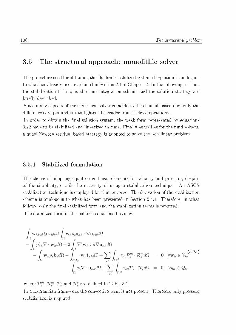
108 The stru tural problem3.5 The stru tural approa h: monolithi solverThe pro edure used for obtaining the algebrai stabilized system of equation is analogousto what has already been explained in Se tion 2.4 of Chapter 2. In the following se tionsthe stabilization te hnique, the time integration s heme and the solution strategy arebriey des ribed.Sin e many aspe ts of the stru tural solver oin ide to the element-based one, only thedieren es are pointed out to lighten the reader from useless repetitions.In order to obtain the nal solution system, the weak form represented by equations3.22 have to be stabilized and linearized in time. Finally as well as for the uid solvers,a quasi-Newton residual based strategy is adopted to solve the non linear problem.3.5.1 Stabilized formulationThe hoi e of adopting equal order linear elements for velo ity and pressure, despiteof the simpli ity, entails the ne essity of using a stabilization te hnique. An ASGSstabilization te hnique is employed for that purpose. The derivation of the stabilizations heme is analogous to what has been presented in Se tion 2.4.1. Therefore, in whatfollows, only the nal stabilized form and the stabilization terms is reported.The stabilized form of the balan e equations be omes∫

Ω

whρs∂tus hdΩ

∫

Ω

whρsas h · ∇us hdΩ

−∫

Ω

p′s h∇ ·whdΩ + 2

∫

Ω

∇swh : µ∇us hdΩ

−∫

Ω

whρsbsdΩ−∫

∂ΩN

whts hdΓ +∑

el

∫

Ωel

τs 1Pms · Rm

s dΩ = 0 ∀wh ∈ Vh,∫

Ω

qh∇ · us hdΩ+∑

el

∫

Ωel

τs 2Pcs · Rc

sdΩ = 0 ∀qh ∈ Qh,

(3.23)where Pm

s , Rms , Pc

s and Rcs are dened in Table 3.1.In a Lagrangian framework the onve tive term is not present. Therefore only pressurestabilization is required.

The stru tural approa h: monolithi solver 109Momentum equation

Pms (wh) as h · ∇wh +∇qh

τs 1

(α

∆t+

4µ

h2 ρs+

2|as h|h

)−1

Rms (us h) ∂tus h + as h · ∇us h −∇ ·

µ

ρs∇sus h +∇p′s h − bsContinuity equation

Pcs (wh) ∇ ·wh

τs 2µ

ρs+

h|as h|2

Rcs(us h) ∇ · us hTable 3.1: Stabilizing elemental terms in ASGS for the non-Newtonian element.3.5.2 Dis retization pro edureA ording to what was explained in Se tion 2.4.2 of Chapter 2, the matrix form of thestabilized system of equations 3.23 an be written as:

[

M+ SMwu 0

0 0

]

·[

us

ps

]

+

[

K+ Swu + Sc G+ Swp

D+ Squ Spq

]

·[

us

ps

]

=

[

Fs + Sfw

Sfq

](3.24)where the operators are expli itly written in Table 3.2 and the stabilization operators an be found in Table 3.3.3.5.3 Bossak time integration s hemeAs in the uid element-based solver, a Bossak time integration s heme is used to advan ein time the momentum equations. For more details about the method see Se tion 2.4.3.Equations 3.24 an be written in ompa t form asMvs + fs int(vs(t), t) = fs ext(t). (3.25)

110 The stru tural problem

Matri ial term Continuum termMus

∑

el

∫

Ωel

whρs∂tus hdΩ

KCus

∑

el

∫

Ωel

whρsas h · ∇us hdΩ

Kus

Kµus +2∑

el

∫

Ωel

wh∇wh : µ∇us hdΩ

Gps −∑

el

∫

Ωel

ps h∇ ·whdΩ

Dus

∑

el

∫

Ωel

qh∇ · us hdΩ

Fs

∑

el

∫

Ωel

whρsbsdΩ

hs 0Table 3.2: Matri es and ve tors of system 3.24 without stabilization terms.

The stru tural approa h: monolithi solver 111Momentum equationMatri ial term Continuum term

SMwuus

∑

el

∫

Ωel

τs1as h · ∇wh∂tus hdΩ

SCwuus

∑

el

∫

Ωel

τs1as h · ∇whas h · ∇us hdΩ

Swuus

Sµwuus −

∑

el

∫

Ωel

τs1as h · ∇wh∇ ·µ

ρs∇sus hdΩ

Swpps

∑

el

∫

Ωel

τs1as h · ∇wh∇ps hdΩ

Sfw −

∑

el

∫

Ωel

τs1as h · ∇whbs hdΩ

SCquus

∑

el

∫

Ωel

τs1∇qhas h · ∇us hdΩ

Squus

Sµquus −

∑

el

∫

Ωel

τ1∇qh∇ ·µ

ρs∇sus hdΩ

Sqpps

∑

el

∫

Ωel

τs1∇qh∇ps hdΩ

Sfq −

∑

el

∫

Ωel

τs1∇qhbs hdΩContinuity equationScus

∑

el

∫

Ωel

τs2∇ ·wh∇ · us hdΩTable 3.3: Stabilization matri es and ve tors of system 3.24.

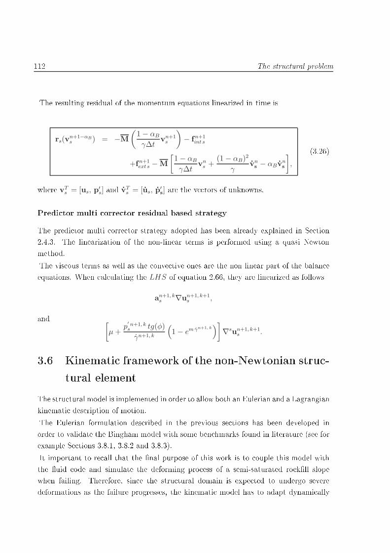
112 The stru tural problemThe resulting residual of the momentum equations linearized in time isrs(v

n+1−αBs ) = −M

(1− αB

γ∆tvn+1s

)

− fn+1int s

+fn+1ext s −M

[1− αB

γ∆tvns +

(1− αB)2

γvns − αBv

ns

]

,

(3.26)where vTs = [us, p

′s] and vT

s = [us, p′s] are the ve tors of unknowns.Predi tor multi orre tor residual based strategyThe predi tor multi orre tor strategy adopted has been already explained in Se tion2.4.3. The linearization of the non-linear terms is performed using a quasi Newtonmethod.The vis ous terms as well as the onve tive ones are the non linear part of the balan eequations. When al ulating the LHS of equation 2.66, they are linearized as follows

an+1, ks ∇un+1, k+1

s ,and [

µ+p′ n+1, ks tg(φ)

γn+1, k

(

1− emγn+1, k)]

∇sun+1, k+1s .3.6 Kinemati framework of the non-Newtonian stru -tural elementThe stru tural model is implemented in order to allow both an Eulerian and a Lagrangiankinemati des ription of motion.The Eulerian formulation des ribed in the previous se tions has been developed inorder to validate the Bingham model with some ben hmarks found in literature (see forexample Se tions 3.8.1, 3.8.2 and 3.8.3).It important to re all that the nal purpose of this work is to ouple this model withthe uid ode and simulate the deforming pro ess of a semi-saturated ro kll slopewhen failing. Therefore, sin e the stru tural domain is expe ted to undergo severedeformations as the failure progresses, the kinemati model has to adapt dynami ally

The parti le nite element method (PFEM) 113to su h deformations leading to the preferable hoi e of a Lagrangian approa h. Amongmany possible Lagrangian methods, the Parti le Finite Element Method (PFEM) hasbeen hosen and implemented for its exibility and reliability [75, 100.3.7 The parti le nite element method (PFEM)The PFEM is a numeri al method that uses a Finite Element mesh to dis retize thephysi al domain and to integrate the dierential governing equations (see [67, 75). InPFEM the domain is modeled using an Updated Lagrangian Formulation. That is allthe variables are assumed to be known in the urrent onguration at time t and theyare brought in the next (or updated) onguration at time t + dt. The nite elementmethod (FEM) is used to solve the ontinuum equations in a mesh built up from theunderlying nodes (the parti les). This is useful to model the separation of solid parti lesfrom the bed surfa e and to follow their subsequent motion as individual parti les witha known density, an initial a eleration and a velo ity subje t to gravity for es [97, 100.It is important to underline that in PFEM ea h parti le is treated as a material point hara terized by the density of the solid domain to whi h it belongs to. The global massis obtained by integrating density at the dierent material points over the domain. Thequality of the numeri al solution depends on the dis retization hosen as in the standardFEM. Adaptive mesh renement te hniques an be used to improve the solution in zoneswhere large gradients of the uid or the stru ture variables o ur.Sin e its rst development espe ially fo used on the simulation of free surfa e owsand breaking waves [67, 75, PFEM has been su essfully used in a wide range of elds.Just to mention some of them, it is used in FSI and oupled problems [68, 95, 98, 99,110, multi-uid problems [65, 84, onta t problems [22, 23, geote hni al simulations[23, 94 and re engineering [19. Moreover PFEM has also been su essfully used inthe implementation of Bingham plasti s model for the simulation of landslides [46 and ement slump tests [45.The basi ingredients of PFEM an be summarized in:• An Updated Lagrangian kinemati al des ription of motion;• A fast remeshing algorithm;• A boundary re ognition method(alpha-shape);

114 The stru tural problem• FEM for the solution of the governing equations;3.7.1 Updated Lagrangian kinemati al des ription of motionThe PFEM was on eived as a Lagrangian method to treat CFD problems in ludingfree surfa e ows and breaking waves [67, 100. This approa h is in ontrast with the lassi al Eulerian way to treat CFD problems.Lagrangian algorithms are traditionally used in stru tural me hani s where ea h nodeof the omputational mesh follows the asso iated material parti le evolution. This isa good way to tra e easily the interfa e between uid and stru ture and to onsidermaterials with history-dependent onstitutive relations. Its weakness is the inability tofollow large distortions of the domain without the ne essity of a ontinuum remeshing.This implies a di ult parallelization of the ode as well.Eulerian algorithms, on the other hand, are largely used in uid dynami s be ause ofthe ease way to follow large movements. In this ase the omputational mesh is xed andthe ontinuum moves with respe t to the grid. Being a xed mesh approa h, an interfa etra king te hnique should be employed in Eulerian methods to follow the evolution ofthe free surfa e (see Se tion 2.6 for more information on the topi ).A third popular te hnique is a generalization of the two kinemati al des ription ofmotion above des ribed. It is known as the Arbitrary Lagrangian- Eulerian (ALE)des ription. In this ase, the mesh is arbitrarily moved with a velo ity uM and thedomain of the mesh is alled the referen e domain [51.For uT

M ≡ (0, 0, 0) an Eulerian onguration is re overed and the referen e domain orresponds to the spatial one. Alternatively, if the mesh velo ity oin ides with theparti le velo ity (uM ≡ u), then the onve tive term disappears and the Lagrangianformulation is re overed. In this ase the referen e domain oin ides with the materialone. The absen e of the onve tive term in a Lagrangian framework, leads also to theelimination of the problems onne ted with onve tion dominating pro esses (see Se tion2.4.1 of Chapter 2), simplifying the stabilization pro edure.A ording to [51, three possible Lagrangian formulations are possible• The total Lagrangian , where variables are des ribed in the initial ongurationΩ0, at time t0;• The updated Lagrangian , where variables are des ribed in the urrent ongurationΩn, at time tn;

The parti le nite element method (PFEM) 115• The end of step Lagrangian , where variables are des ribed in the ongurationΩn+1 at time tn+1.The total Lagrangian formulation is not the best hoi e for a problem with large domaindeformations. Therefore, PFEM uses an updated Lagrangian des ription of motion.3.7.2 Remeshing algorithmThe need of an e ient remeshing algorithm together with the the di ulty of paral-lelizing this pro edure are the biggest drawba k of a Lagrangian approa h.The mesh moves in a ordan e to the material points and large deformations o ur.The ode developed in this work uses external libraries to remesh the domain. They arethe TetGen and Triangle for the 2D and the 3D ases respe tively (for more informationsee [5).The mesh generation s heme is based on the Voronoi diagrams1 and the Delaunaytessellation2.3.7.3 Boundary re ognition method: alpha - shape methodOn e the ontinuum domain is partitioned using the TetGen library, a riteria is neededto dene the free surfa es and the boundaries on the material domain. In the ase ofPFEM, alpha shape [20 is the adopted te hnology.Ea h node i of the domain has its own dimension hi determined as the average distan eof node i from its neighbors. In the same way, an elemental dimension hel an be denedfor ea h element as the average of the hi of its nodes. Finally depending on the pre isionwanted, an α ustom parameter greater but lose to one (the alpha shape parameter) isdened.If the radius of the sphere that ir ums ribes the element (r) is bigger than α ·hel, thenthe element is eliminated (see Figure 3.4). That is1 The Voronoi diagram of a setN is a partition of R3 into region Vi ( losed and onvex or unbounded),where ea h region Vi is asso iated with a node pi, su h that any point in Vi is loser to pi than to anyother node pj . The Voronoi diagram is unique.2 A Delaunay tessellation within the set N is a partition of the onvex hull Ω of all the nodesinto region Ωi su h that Ω = Ωi where ea h Ωi is the tetrahedron dened by 4 nodes of the sameVoronoi sphere. A Voronoi sphere within the set N is any sphere, dened by 4 or more nodes, that ontains no other node inside. Su h sphere are otherwise known as empty ir umspheres. The Delaunaytriangulation and Voronoi diagram in R

2 are dual to ea h other in the graph theoreti al sense.

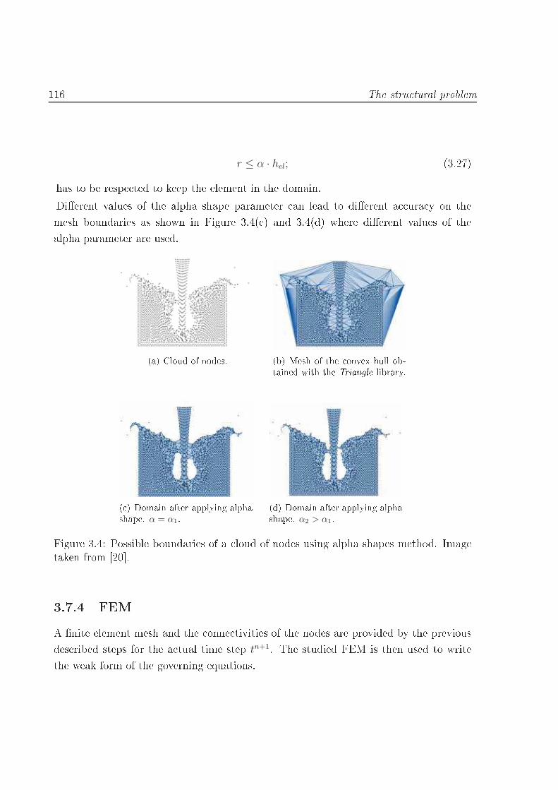
116 The stru tural problemr ≤ α · hel; (3.27)has to be respe ted to keep the element in the domain.Dierent values of the alpha shape parameter an lead to dierent a ura y on themesh boundaries as shown in Figure 3.4( ) and 3.4(d) where dierent values of thealpha parameter are used.

(a) Cloud of nodes. (b) Mesh of the onvex hull ob-tained with the Triangle library.( ) Domain after applying alphashape. α = α1. (d) Domain after applying alphashape. α2 > α1.Figure 3.4: Possible boundaries of a loud of nodes using alpha shapes method. Imagetaken from [20.3.7.4 FEMA nite element mesh and the onne tivities of the nodes are provided by the previousdes ribed steps for the a tual time step tn+1. The studied FEM is then used to writethe weak form of the governing equations.

Numeri al Examples 1173.7.5 PFEM algorithmConsidering known the solution at time step n, the basi steps of PFEM algorithm aresummarized in the box that follows.PFEM algorithm1. Imposition of mesh velo ity at time step n usM = un;2. Lapla ian smoothing a (free surfa e kept xed);3. Remesh (see Se tion 3.7.2);4. Solve the monolithi system;5. Ba k to step 1.aThe Lapla ian smoothing is a geometri al te hnique that allows a more homogeneousredistribution of the nodes inside the analysis domain without hanging the onne tivitiesbetween nodes3.8 Numeri al Examples3.8.1 The Couette owThe Couette ow refers to the laminar ow of a vis ous uid between two parallel inniteplates separated by a given distan e, one of whi h is moving relative to the other. Theow is driven by virtue of vis ous drag for e a ting on the uid and the applied pressuregradient parallel to the plates.The modelThe length of the omputational domain is 6m and its height is 1m as shown in Figure3.5. The Neumann boundary onditions are applied on the verti al edges in terms ofexternal pressure. Diri hlet onditions are then applied on the horizontal edges (theplates). The lower plate is onsidered xed, whereas the upper moves with a onstanthorizontal velo ity. The horizontal velo ity diagram in the entral verti al se tion isanalyzed.

118 The stru tural problem6m

1m

DENSITY = 1 kg/mcVISCOSITY = 10 Pas

IMPOSED vx

FIXED EDGE

EXTERNAL RIGHT

PRESSURE

EXTERNAL LEFT

PRESSURE

Figure 3.5: Geometri al data and boundary onditions.Figure 3.6: Linear triangular mesh used in the al ulation.The mesh used in every model is shown in Figure 3.6. It has 14736 linear triangularelements. Their dimension varies from 0.05m at the sides to 0.01m in the entral verti alse tion.The numeri al resultsIn all the numeri al examples the value of m and τ0 are kept onstant as well as theproperties of the material. They are summarized in Table 3.4.Density ρs 1kg/m3Fluidied vis osity µ 10Pa sSmoothing oe ient m 300sYield stress τ0 10PaTable 3.4: Couette example. Material properties.Figure 3.7 shows the used regularized approximation in omparison with the bilinearform.The dieren e between the ee ts of a positive pressure gradient (adverse to the velo ityeld) and a negative one (favorable to the velo ity eld) are shown in Figure 3.9. In both

Numeri al Examples 119

0.00 0.05 0.10 0.15 0.20Shear Rate

0

20

40

60

80

100

120

Shea

r Str

ess

[Pa]

Bingham exponential approximationBingham bilinear lawFigure 3.7: Exponential approximation with m=300 and τ0 = 100Pa. ases an in reasing gradient of pressure is taken into a ount. The velo ity of the upperplate is ux = 0.5m/s. The gradient of velo ity is higher lose to the plate. Consequentlythe value of tangential stress is also higher in these zones that are the regions where theyield stress is a hieved. The entral straight zone is the unyielded region where γ = 0and µ = µ + τ0 ·m. The vis osity behavior in the entral verti al se tion is shown inFigure 3.8

0 5000 10000 15000 20000 25000 30000 35000Apparent Viscosity [Pas]

0.0

0.2

0.4

0.6

0.8

1.0

Vert

ical

pos

ition

[m]

Figure 3.8: Variation f vis osity in the entral verti al se tion.In reasing the gradient of pressure the rigid plateau is narrowing and the yielded zoneis in reasing.Finally, the upper velo ity is set to ux = 0.01m/s to reprodu e the results of [105and to have a dire t omparison with the analyti al results as shown in Figure 3.10.

120 The stru tural problem

0 1 2 3 4 5 6 7 8 9Velocity [m/s]

0.0

0.2

0.4

0.6

0.8

1.0

Vert

ical

pos

ition

[m]

Non-Newtonian Flow with upper Vx=0.5m/s and negative Dp.

Dp 500Pa/mDp 666.67Pa/mDp 833.33Pa/mDp 1000Pa/m

(a) Negative Pressure Gradient 87654321 0 1Velocity [m/s]

0.0

0.2

0.4

0.6

0.8

1.0

Vert

ical

pos

ition

[m]

Non-Newtonian Flow with upper Vx=0.5m/s and positive Dp.

Dp 500Pa/mDp 666.67Pa/mDp 833.33Pa/mDp 1000Pa/m

(b) Positive Pressure GradientFigure 3.9: Velo ity diagrams for dierent values of the gradient of pressure. Upperhorizontal velo ity 0.5m/s.Dierent values of negative gradients of pressure are onsidered as shown in Figure 3.10.Right edge external pressure is kept onstant and equal to 0Pa in all the ases, whereasthe left hand side pressure is 1500Pa, 1600Pa, 1700Pa, 1800Pa, 1900Pa and 2000Parespe tively. The agreement is good and the yield point is reprodu ed orre tly for allthe pressure gradients.

0.0 0.1 0.2 0.3 0.4 0.5 0.6 0.7Velocity [m/s]

0.0

0.2

0.4

0.6

0.8

1.0

Vert

ical

pos

ition

[m]

Dp=

-250.00Pa/m

Dp=

-266.67Pa/m

Dp=

-283.33Pa/m

Dp=

-300.00Pa/m

Dp=

-316.67Pa/m

Dp=

-333.33Pa/m

Non-Newtonian Flow with upper Vx 0.01m/s and negative Dp.

NumericalAnalyticalFigure 3.10: Velo ity diagrams for dierent values of a negative gradient of pressure.Upper horizontal velo ity 0.01m/s.

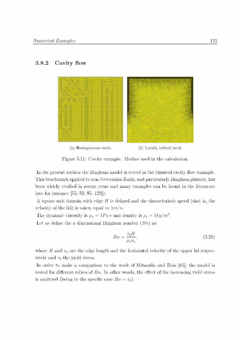
Numeri al Examples 1213.8.2 Cavity ow

(a) Homogeneous mesh. (b) Lo ally rened mesh.Figure 3.11: Cavity example. Meshes used in the al ulation.In the present se tion the Bingham model is tested in the lassi al avity ow example.This ben hmark applied to non-Newtonian uids, and parti ularly Bingham plasti s, hasbeen widely studied in re ent years and many examples an be found in the literature(see for instan e [55, 59, 85, 129).A square unit domain with edge H is dened and the hara teristi speed (that is, thevelo ity of the lid) is taken equal to 1m/s.The dynami vis osity is µs = 1Pa s and density is ρs = 1kg/m3.Let us dene the a dimensional Bingham number (Bn) asBn =

τ0H

µsus, (3.28)where H and us are the edge length and the horizontal velo ity of the upper lid respe -tively and τ0 the yield stress.In order to make a omparison to the work of Mitsoulis and Zisis [85, the model istested for dierent values of Bn. In other words, the ee t of the in reasing yield stressis analyzed (being in the spe i ase Bn = τ0).

122 The stru tural problem

(a) Homogeneous mesh. (b) Lo ally rened mesh.Figure 3.12: Cavity. White olor shows the yielded regions. Comparison between the ase with homogeneous mesh (Figure 3.11(a)) and the rened one (Figure 3.11(b)).

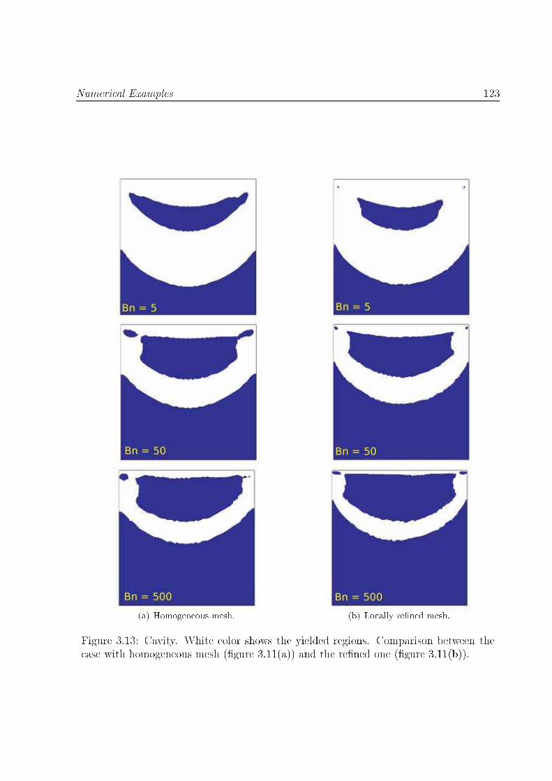
Numeri al Examples 123

(a) Homogeneous mesh. (b) Lo ally rened mesh.Figure 3.13: Cavity. White olor shows the yielded regions. Comparison between the ase with homogeneous mesh (gure 3.11(a)) and the rened one (gure 3.11(b)).

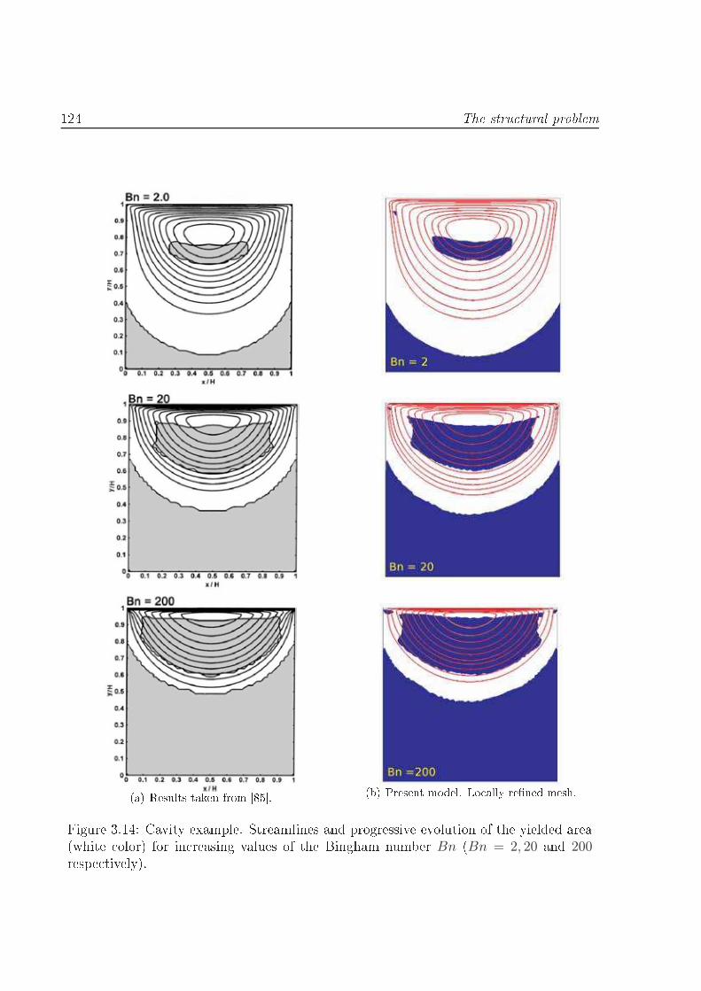
124 The stru tural problem

(a) Results taken from [85. (b) Present model. Lo ally rened mesh.Figure 3.14: Cavity example. Streamlines and progressive evolution of the yielded area(white olor) for in reasing values of the Bingham number Bn (Bn = 2, 20 and 200respe tively).

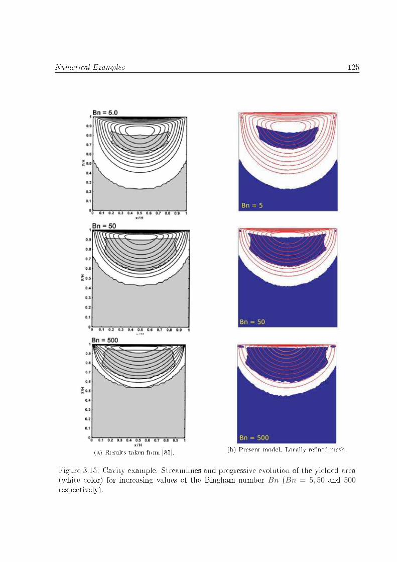
Numeri al Examples 125

(a) Results taken from [85. (b) Present model. Lo ally rened mesh.Figure 3.15: Cavity example. Streamlines and progressive evolution of the yielded area(white olor) for in reasing values of the Bingham number Bn (Bn = 5, 50 and 500respe tively).

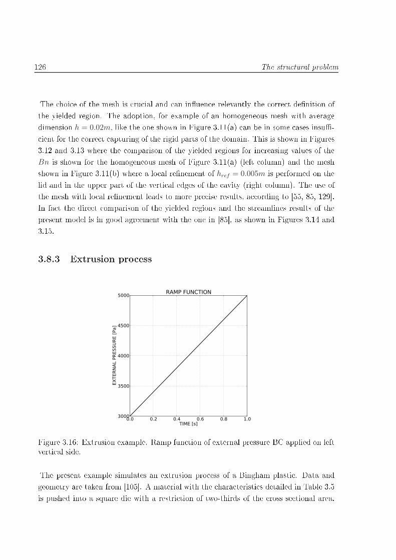
126 The stru tural problemThe hoi e of the mesh is ru ial and an inuen e relevantly the orre t denition ofthe yielded region. The adoption, for example of an homogeneous mesh with averagedimension h = 0.02m, like the one shown in Figure 3.11(a) an be in some ases insu- ient for the orre t apturing of the rigid parts of the domain. This is shown in Figures3.12 and 3.13 where the omparison of the yielded regions for in reasing values of theBn is shown for the homogeneous mesh of Figure 3.11(a) (left olumn) and the meshshown in Figure 3.11(b) where a lo al renement of href = 0.005m is performed on thelid and in the upper part of the verti al edges of the avity (right olumn). The use ofthe mesh with lo al renement leads to more pre ise results, a ording to [55, 85, 129.In fa t the dire t omparison of the yielded regions and the streamlines results of thepresent model is in good agreement with the one in [85, as shown in Figures 3.14 and3.15.3.8.3 Extrusion pro ess

0.0 0.2 0.4 0.6 0.8 1.0TIME [s]

3000

3500

4000

4500

5000

EXTE

RNAL

PRE

SSUR

E [P

a]

RAMP FUNCTION

Figure 3.16: Extrusion example. Ramp fun tion of external pressure BC applied on leftverti al side.The present example simulates an extrusion pro ess of a Bingham plasti . Data andgeometry are taken from [105. A material with the hara teristi s detailed in Table 3.5is pushed into a square die with a restri tion of two-thirds of the ross se tional area.

Numeri al Examples 127Due to the symmetry of the problem, only half of the domain is al ulated as shown inFigure 3.17. An in reasing value of the external pressure (pext) is imposed on the leftside with a pressure in rement of 2Pa/step (the ramp fun tion for applying the externalboundary pressure is detailed in Figure 3.16). On the right side the external pressure isset to zero and kept onstant. The walls are assumed to be fri tionless.Pext(

t)

AB

6m 6m

2m

1m

SLIP B.C.

SLIP B.C.

SLIP

B.C

.

Pext = 0PaFigure 3.17: Extrusion example. Geometry and boundary onditions.Figure 3.18: Extrusion example. Mesh used in the al ulation. Average dimensionh = 0.2m with a lo al renement 0.05m near point B of Figure 3.17 and in the restri tionarea and an additional renement 0.005m lose to point A of Figure 3.17. The totalnumber of triangular elements and nodes are 11 600 and 5 800, respe tively.The mesh used in the al ulation is shown in Figure 3.18. It is rened in the area ofappearan e of the slip lines to a urately at h their evolution.As explained in [105, in the hypothesis of perfe t plasti ity, the value of maximum rampressure (pmax

ext ) is analyti ally al ulated in [82. It is given by the following relationpmaxext =

4

3

[

1 +π

2

]

τ0 = 3426.7Pa. (3.29)This is the analyti al yield pressure, whi h orresponds numeri ally to the time intervalbetween the onset of the slip line an its full development. In the present model this isrepresented by the interval in whi h the external pressure is between 3418Pa (beginningof the formation of the slip line) and 3472Pa (the slip line is fully formed). The analyti al

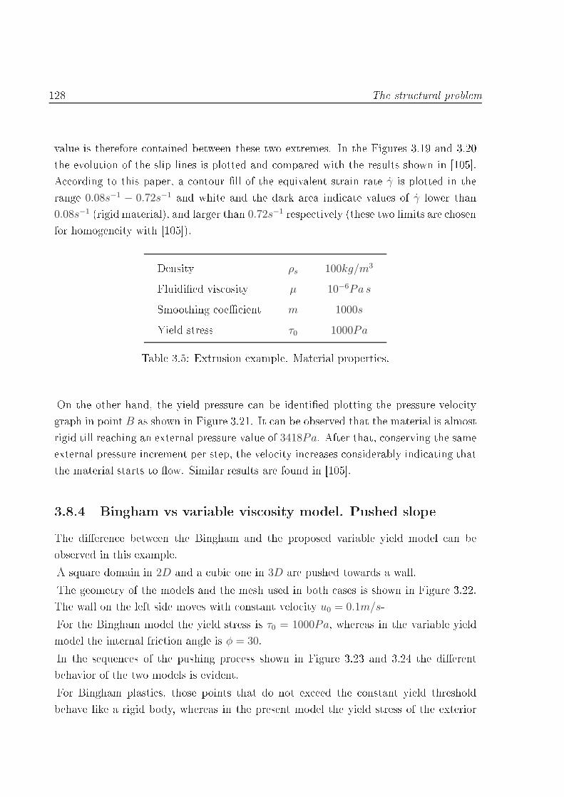
128 The stru tural problemvalue is therefore ontained between these two extremes. In the Figures 3.19 and 3.20the evolution of the slip lines is plotted and ompared with the results shown in [105.A ording to this paper, a ontour ll of the equivalent strain rate γ is plotted in therange 0.08s−1 − 0.72s−1 and white and the dark area indi ate values of γ lower than0.08s−1 (rigid material), and larger than 0.72s−1 respe tively (these two limits are hosenfor homogeneity with [105).Density ρs 100kg/m3Fluidied vis osity µ 10−6Pa sSmoothing oe ient m 1000sYield stress τ0 1000PaTable 3.5: Extrusion example. Material properties.On the other hand, the yield pressure an be identied plotting the pressure-velo itygraph in point B as shown in Figure 3.21. It an be observed that the material is almostrigid till rea hing an external pressure value of 3418Pa. After that, onserving the sameexternal pressure in rement per step, the velo ity in reases onsiderably indi ating thatthe material starts to ow. Similar results are found in [105.3.8.4 Bingham vs variable vis osity model. Pushed slopeThe dieren e between the Bingham and the proposed variable yield model an beobserved in this example.A square domain in 2D and a ubi one in 3D are pushed towards a wall.The geometry of the models and the mesh used in both ases is shown in Figure 3.22.The wall on the left side moves with onstant velo ity u0 = 0.1m/s-For the Bingham model the yield stress is τ0 = 1000Pa, whereas in the variable yieldmodel the internal fri tion angle is φ = 30.In the sequen es of the pushing pro ess shown in Figure 3.23 and 3.24 the dierentbehavior of the two models is evident.For Bingham plasti s, those points that do not ex eed the onstant yield thresholdbehave like a rigid body, whereas in the present model the yield stress of the exterior

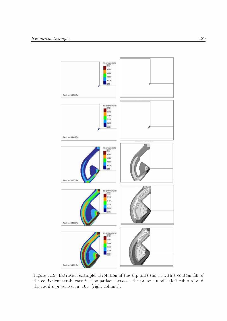
Numeri al Examples 129

Figure 3.19: Extrusion example. Evolution of the slip lines shown with a ontour ll ofthe equivalent strain rate γ. Comparison between the present model (left olumn) andthe results presented in [105 (right olumn).

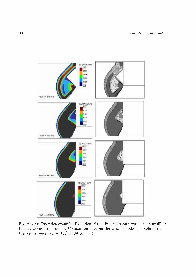
130 The stru tural problem

Figure 3.20: Extrusion example. Evolution of the slip lines shown with a ontour ll ofthe equivalent strain rate γ. Comparison between the present model (left olumn) andthe results presented in [105 (right olumn).

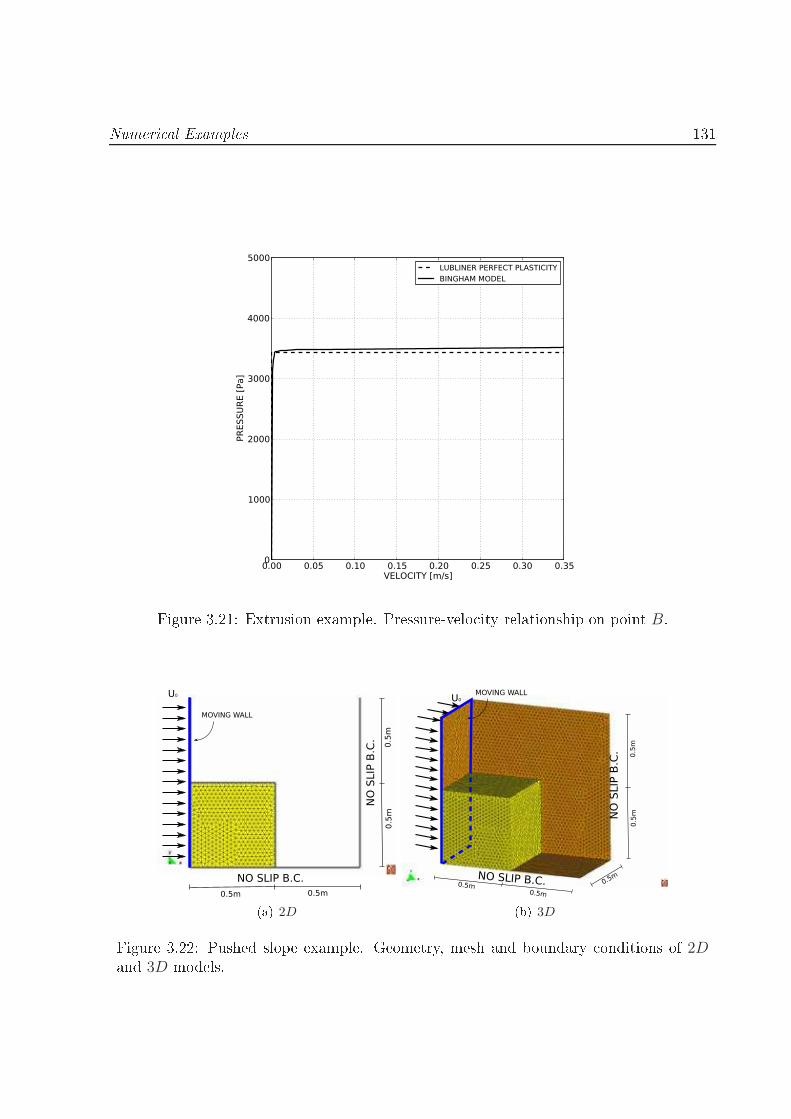
Numeri al Examples 131

0.00 0.05 0.10 0.15 0.20 0.25 0.30 0.35VELOCITY [m/s]

0

1000

2000

3000

4000

5000

PRES

SURE

[Pa]

LUBLINER PERFECT PLASTICITYBINGHAM MODEL

Figure 3.21: Extrusion example. Pressure-velo ity relationship on point B.

NO SLIP B.C.

NO

SLIP

B.C

.

U0

MOVING WALL

0.5

m0.5

m

0.5m 0.5m(a) 2D

NO SLIP B.C.

NO

SLIP

B.C

.

U0

MOVING WALL

0.5m0.5m

0.5m

0.5

m0

.5m

(b) 3DFigure 3.22: Pushed slope example. Geometry, mesh and boundary onditions of 2Dand 3D models.

132 The stru tural problemDry density ρs 1000kg/m3Fluidied vis osity µ 10−6Pa sSmoothing oe ient m 3000sTable 3.6: Pushed slope example. Material properties.points is lower and it is ex eeded also for lower pressure levels. Two dierent phases anbe identied in the present example:- The settlement phase. It is the initial part of the example. The granular materialis left free to fall and to rea h its stable onguration. It goes from the beginningof the example to the moment in whi h the material tou hes the right xed wall.- The squeezing phase. It begins when the material tou hes the right wall and startsto be squeezed between the two opposite walls that are getting loser.In Figure 3.23 the 2D omparison between the Bingham model and the variable yieldmodel during the settlement phase is shown. The ontour ll of the equivalent strainrate is plotted in dierent time instan es (the blue olor indi ates γ = 0).The Bingham model shows a sliding surfa e where the tangential stress rea hes theyield stress (1000Pa), whereas all the rest of the model shows an almost rigid behavior.Conversely, in the variable yield model, if a node has a tangential stress whi h ex eed itspressure times the fri tion angle tangent (pstgφ), it shows a drop in the vis osity and itstarts owing. The main dieren es an be observed on the free surfa e where the yieldstress tends to zero the loser the node is to the free surfa e (where the pressure is zero),i.e. no resistan e is present. The variable yield material rea hes a stable ongurationthat respe ts the internal fri tion angle of 30. For more details the onsultation ofSe tion 3.8.5 is re ommended.In Figure 3.24 the behavior of the two models in the squeezing phase is ompared. Thesequen e shows how the equivalent strain rate γ is almost zero up to the reation of thefailure lines and the subsequent ollapse of the material. In the granular material onthe ontrary, the free surfa e has zero pressure, whi h implies zero resistan e and assoon as the material rea hes the height of the walls it starts falling.The same onsiderations an be done in 3D, looking at the omparison between thetwo models in the settlement and the squeezing phase shown in Figures 3.25 and 3.26,

Numeri al Examples 133

(a) Bingham model. (b) Variable yield model.Figure 3.23: 2D pushed slope. γ in the initial pushing phase. Dieren e between theBingham and the variable vis osity models.respe tively. The Bingham model in 3D shows less resistan e in the squeezing phasedue to the 3-dimensional ee ts. It is nally interesting to observe that the materialwhi h is falling down in the ase of the Bingham model onserves the velo ity imposed

134 The stru tural problem

(a) Bingham model. (b) Variable yield model.Figure 3.24: 2D pushed slope. γ in the squeezing phase. Dieren e between the Bing-ham and the variable vis osity models.by the wall although this is very low, whereas this does not happen in the variable yieldmodel.

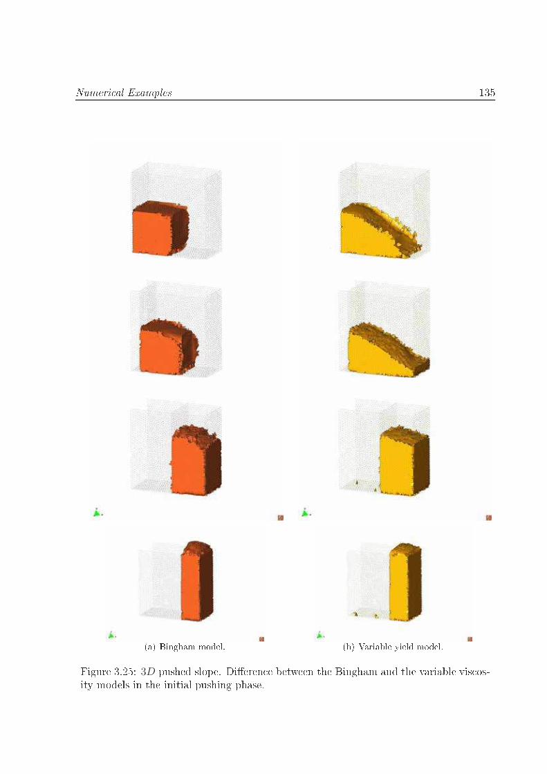
Numeri al Examples 135

(a) Bingham model. (b) Variable yield model.Figure 3.25: 3D pushed slope. Dieren e between the Bingham and the variable vis os-ity models in the initial pushing phase.

136 The stru tural problem

(a) Bingham model. (b) Variable yield model.Figure 3.26: 3D pushed slope. Dieren e between the Bingham and the variable vis os-ity models in the squeezing phase.

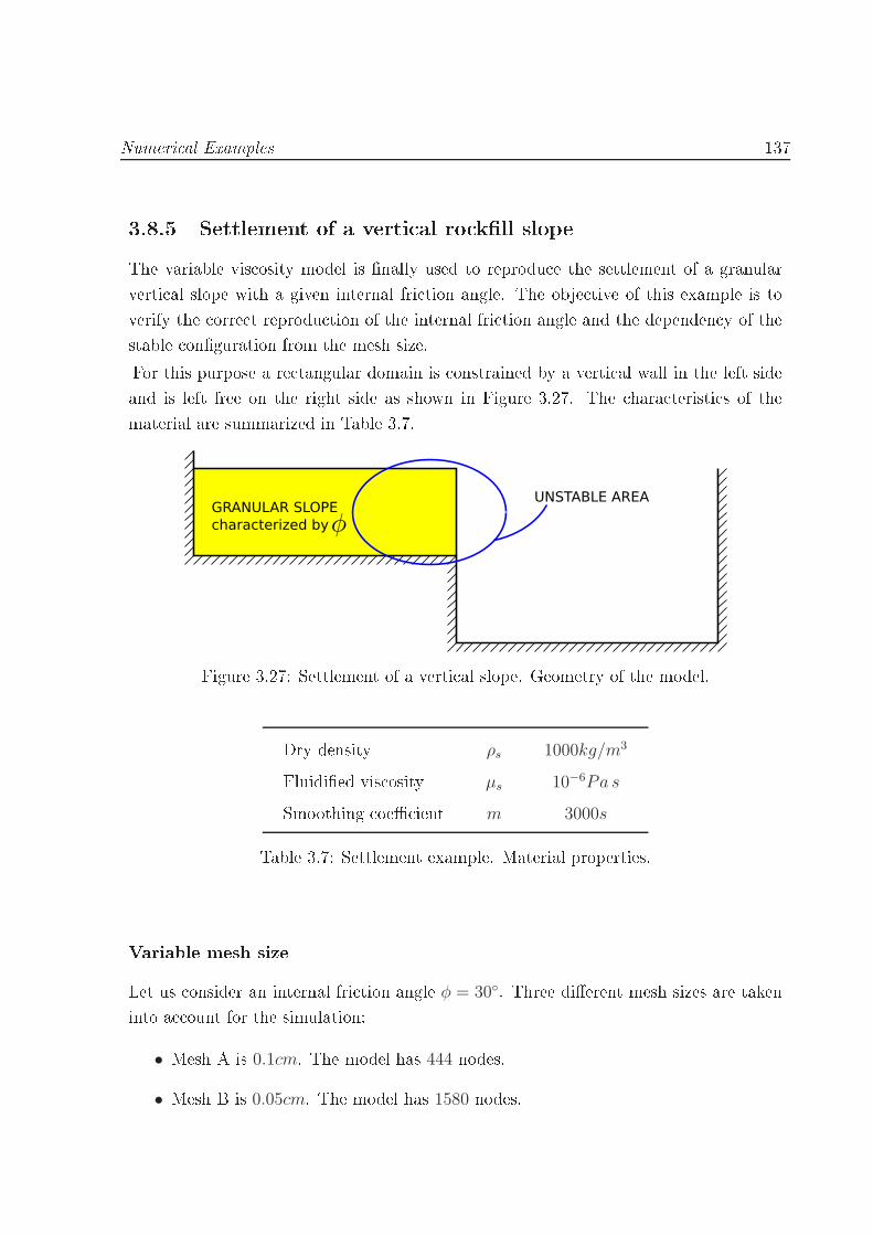
Numeri al Examples 1373.8.5 Settlement of a verti al ro kll slopeThe variable vis osity model is nally used to reprodu e the settlement of a granularverti al slope with a given internal fri tion angle. The obje tive of this example is toverify the orre t reprodu tion of the internal fri tion angle and the dependen y of thestable onguration from the mesh size.For this purpose a re tangular domain is onstrained by a verti al wall in the left sideand is left free on the right side as shown in Figure 3.27. The hara teristi s of thematerial are summarized in Table 3.7.UNSTABLE AREA

GRANULAR SLOPE

characterized by

Figure 3.27: Settlement of a verti al slope. Geometry of the model.Dry density ρs 1000kg/m3Fluidied vis osity µs 10−6Pa sSmoothing oe ient m 3000sTable 3.7: Settlement example. Material properties.Variable mesh sizeLet us onsider an internal fri tion angle φ = 30. Three dierent mesh sizes are takeninto a ount for the simulation:• Mesh A is 0.1cm. The model has 444 nodes.• Mesh B is 0.05cm. The model has 1580 nodes.

138 The stru tural problem• Mesh C is 0.01cm. The model has 35466 nodes.They are shown in Figure 3.28.

(a) Mesh A 0.1m.(b) Mesh B 0.05m.( ) Mesh C 0.01m.Figure 3.28: Dierent mesh sizes taken into a ount in the present example.The evolution of the settlement is shown in Figure 3.29 for the above mentioned meshes.As expe ted the more a urate and realisti settlement pro ess is obtained with the nermesh but no relevant dieren es appear using the oarser ones. This is respe ted forany internal fri tion angle φ less than 45. In fa t in the latter ase the orre t behaviorof the material is inuen ed by the mesh size. For oarse meshes the material behavesas rigid as shown in Figure 3.30 where two meshes are taken into a ount. However inthe next se tion it will be pointed out that this value of φ is in the limit of validity ofthe model.

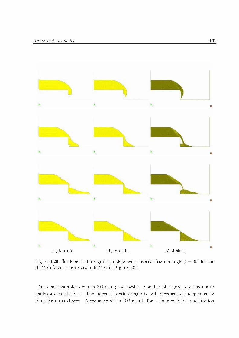
Numeri al Examples 139

(a) Mesh A. (b) Mesh B. ( ) Mesh C.Figure 3.29: Settlements for a granular slope with internal fri tion angle φ = 30 for thethree dierent mesh sizes indi ated in Figure 3.28.The same example is run in 3D using the meshes A and B of Figure 3.28 leading toanalogous on lusions. The internal fri tion angle is well represented independentlyfrom the mesh hosen. A sequen e of the 3D results for a slope with internal fri tion

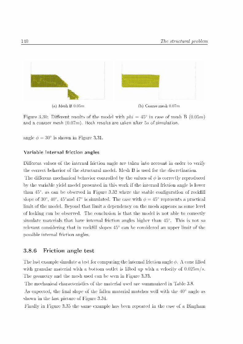
140 The stru tural problem

(a) Mesh B 0.05m (b) Coarse mesh 0.07mFigure 3.30: Dierent results of the model with phi = 45 in ase of mesh B (0.05m)and a oarser mesh (0.07m). Both results are taken after 5s of simulation.angle φ = 30 is shown in Figure 3.31.Variable internal fri tion anglesDierent values of the internal fri tion angle are taken into a ount in order to verifythe orre t behavior of the stru tural model. Mesh B is used for the dis retization.The dierent me hani al behavior ontrolled by the values of φ is orre tly reprodu edby the variable yield model presented in this work if the internal fri tion angle is lowerthan 45, as an be observed in Figure 3.32 where the stable onguration of ro kllslope of 30, 40, 45and 47 is simulated. The ase with φ = 45 represents a pra ti allimit of the model. Beyond that limit a dependen y on the mesh appears as some levelof lo king an be observed. The on lusion is that the model is not able to orre tlysimulate materials that have internal fri tion angles higher than 45. This is not sorelevant onsidering that in ro kll slopes 45 an be onsidered an upper limit of thepossible internal fri tion angles.3.8.6 Fri tion angle testThe last example simulate a test for omputing the internal fri tion angle φ. A one lledwith granular material with a bottom outlet is lifted up with a velo ity of 0.025m/s.The geometry and the mesh used an be seen in Figure 3.33.The me hani al hara teristi s of the material used are summarized in Table 3.8.As expe ted, the nal slope of the fallen material mat hes well with the 40 angle asshown in the last pi ture of Figure 3.34.Finally in Figure 3.35 the same example has been repeated in the ase of a Bingham

Numeri al Examples 141

30º

(a) Mesh A.30º

(b) Mesh B.Figure 3.31: Settlements for a 3D granular slope with internal fri tion angle φ = 30 inthe ase of onsidering mesh A and B of Figure 3.28.plasti with a yield threshold τ0 = 500Pa.The dierent behaviour between the two models is evident: the material of the variableyield model ows down in a nearly ontinuous way and at the end of the simulation no

142 The stru tural problem

(a) φ = 30 (b) φ = 40

( ) φ = 45 (d) φ = 47Figure 3.32: Stable results for dierent internal fri tion angles φ. The mesh used in the al ulation is mesh B of Figure 3.28.Dry density ρs 1490kg/m3Internal fri tion angle ϕ 40Fluidied vis osity µ 10−6Pa sSmoothing oe ient m 3000sTable 3.8: Fri tion angle test example. Material properties.

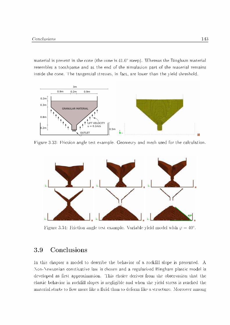
Con lusions 143material is present in the one (the one is 41.6 steep). Whereas the Bingham materialresembles a toothpaste and at the end of the simulation part of the material remainsinside the one. The tangential stresses, in fa t, are lower than the yield threshold.GRANULAR MATERIAL

OUTLET

LIFT VELOCITY

u = 0.1m/s

3m

0.5m

0.9m 0.2m 0.9m

0.2m

0.8m

0.3m

0.2m

Figure 3.33: Fri tion angle test example. Geometry and mesh used for the al ulation.

40ºFigure 3.34: Fri tion angle test example. Variable yield model with ϕ = 40.3.9 Con lusionsIn this hapter a model to des ribe the behavior of a ro kll slope is presented. ANon-Newtonian onstitutive law is hosen and a regularized Bingham plasti model isdeveloped as rst approximation. This hoi e derives from the observation that theelasti behavior in ro kll slopes is negligible and when the yield stress is rea hed thematerial starts to ow more like a uid than to deform like a stru ture. Moreover among

144 The stru tural problem

Figure 3.35: Fri tion angle test example. Bingham model with yield stress τ0 = 500Pa.the non-Newtonian uids, Bingham plasti s have the apability of supporting a ertainamount of shear stress before rea hing large strains.The good behavior of the Bingham model is veried through some ben hmarks, butdoes not seem to be adequate for the simulation of the behavior of a granular slope. Forthis purpose a variable yield threshold is introdu ed in order to mimi a Mohr Coulombfailure riterion.The dieren es between the regularized Bingham and the variable yield models aredis ussed in some examples.The main advantage of the onstitutive law proposed is its simpli ity ompared with anyother plasti model. The treatment of the granular material as a uid leads to balan eequations similar to those presented in Chapter 2. Hen e, most onsiderations alreadydone for the uid model an be used in this ontext as well, providing the ne essaryadaptation to non-Newtonian materials.The variable yield model does not present serious limitations on the mesh sizes in general(although in Chapter 5 it will be pointed out that this is not always true in pra ti al ases). Finally the variable yield model seems to be adequate to simulate materialswith internal fri tion angles lower than 45. Fortunately this value is higher than themaximum threshold of non ohesive ro kll slopes.

Chapter 4The ouplingIn this hapter the oupled model for uid-stru ture intera tion analysis is presented.First the uid and the stru tural balan e equations, already dis ussed in the previousparts of this work, are derived from the monolithi oupled system. A staggered solutionstrategy is adopted to ouple the Eulerian uid solver and the Lagrangian stru tural one.A simple example is presented to he k the orre t behaviour of the algorithm. Finallyin order to fully des ribe the oupling algorithm, the proje tion tool reated to mapinformation between the uid and the stru tural non-mat hing meshes is dis ussed.Additional examples of the appli ation of the oupled analysis method are shown inChapter 5.4.1 Introdu tionThe stru tural stability of ro kll slopes is heavily inuen ed by its intera tion withwater. Traditionally the oupled problem of soils or ro k and water is fa ed using amultiphase material whose behavior is governed by the oupling between the dierentphases: soil, water and air. The rst mathemati al models des ribing the oupling solidand uid phase were developed by Biot [13, 14. Nevertheless his work was suitableonly for linear elasti materials and its extension to non-linear problems with largedeformations was rst arried on by Zienkiewi z and Shiomi only several years later[131. Its should be mentioned that re ently important steps ahead in this eldhavebeen made by Lewis and S hreer [78, Coussy [91 and Boer [49.These lassi al and well established approa hes in geome hani s were not onsidered as

146 The ouplingan alternative in the present work for the following reasons:• The possibility of a urately following the dynami hange of the ow throughoutand over the ro kll is the key point of the model. The oupling of these twophenomena ould be very hallenging in the traditional models needing the trans-ferring of interfa e onditions between the free surfa e problem and the seepageone in order to perform the oupling. On the ontrary, in the present work this isautomati ally taken into a ount, as explained in Chapter 2.• The onsideration of the saturation level and of the intera tion between air andwater in the partially saturated pores, be omes an useless information. In fa t a - ording to experimental eviden e, the problem of interest an always be onsideredfully drained, being the pores inter onne ted.• Due to the time s ale of the ex eptional ooding that an be of the order of minutesor hours, the dam material an be onsidered as rigid (avoiding any elasti responsein the unyielded region) and its ompressibility an be negle ted.• The apability of tra king the material yield surfa e is not needed as ommentedin Chapter 3.The need of developing an ad ho uid approa h for the simulation of the free surfa e-seepage problem des ribed in Chapter 2 leads, as a natural onsequen e, to the hoi e of astaggered strategy. Nevertheless for a onsistent formulation both the uid and stru turebalan e equations should be derived from the imposition of the global equilibrium. Forthat purpose, in the following se tions the monolithi global problem is used to obtainthe balan e equations for the stru ture. In this ase, the equation dis ussed in Chapter3 are ompleted with the oupling terms deriving from the global equilibrium.On e the uid and the stru tural problems are dened, the oupling strategy is pre-sented. The need of working with an Eulerian and a Lagrangian model leads to imple-ment a fully staggered expli it s heme. A key point of the oupled tool is the possibilityof transferring information between the moving and the xed mesh. For su h purposea mapping between non mat hing meshes has been developed. The performan e of thetool is presented at the end of the hapter.

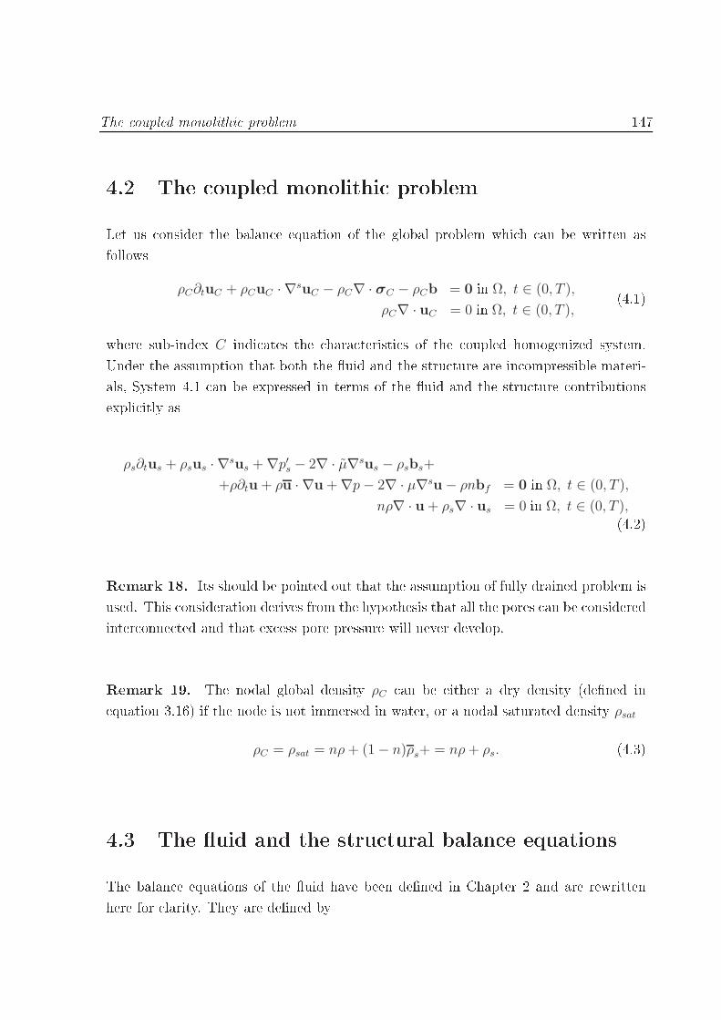
The oupled monolithi problem 1474.2 The oupled monolithi problemLet us onsider the balan e equation of the global problem whi h an be written asfollowsρC∂tuC + ρCuC · ∇suC − ρC∇ · σC − ρCb = 0 in Ω, t ∈ (0, T ),

ρC∇ · uC = 0 in Ω, t ∈ (0, T ),(4.1)where sub-index C indi ates the hara teristi s of the oupled homogenized system.Under the assumption that both the uid and the stru ture are in ompressible materi-als, System 4.1 an be expressed in terms of the uid and the stru ture ontributionsexpli itly as

ρs∂tus + ρsus · ∇sus +∇p′s − 2∇ · µ∇sus − ρsbs+

+ρ∂tu+ ρu · ∇u+∇p− 2∇ · µ∇su− ρnbf = 0 in Ω, t ∈ (0, T ),

nρ∇ · u+ ρs∇ · us = 0 in Ω, t ∈ (0, T ),(4.2)Remark 18. Its should be pointed out that the assumption of fully drained problem isused. This onsideration derives from the hypothesis that all the pores an be onsideredinter onne ted and that ex ess pore pressure will never develop.Remark 19. The nodal global density ρC an be either a dry density (dened inequation 3.16) if the node is not immersed in water, or a nodal saturated density ρsat

ρC = ρsat = nρ+ (1− n)ρs+ = nρ+ ρs. (4.3)4.3 The uid and the stru tural balan e equationsThe balan e equations of the uid have been dened in Chapter 2 and are rewrittenhere for larity. They are dened by

148 The ouplingFluid problem

ρ∂tu+ ρu · ∇u + n∇p− 2∇ · µ∇su

−ρnb +D = 0 in Ω, t ∈ (0, T );

∇ · u = 0 in Ω, t ∈ (0, T );

(4.4)u(x, 0) = u0(x) in Ω;

u(x, t) = g(x, t) on ∂ΩD, t ∈ (0, T );

n · σ(x, t) = t(x, t) on ∂ΩN , t ∈ (0, T );

(4.5)Therefore the equations governing the stru tural problem an be obtained subtra ting4.4 from 4.2. The stru tural system obtained is

ρs∂tus + ρsus · ∇sus +∇p′s−2∇ · µs∇us − ρsb+ (1− n)∇pf −D = 0 in Ωs, t ∈ (0, T ),

∇ · us = 0 in Ωs, t ∈ (0, T ).

(4.6)Stru tural problemρs∂tus + ρsus · ∇sus +∇p′s

−2∇ · µs∇us − ρsb+ (1− n)∇p−D = 0 in Ωs, t ∈ (0, T ),

∇ · us = 0 in Ωs, t ∈ (0, T ),

(4.7)us(x, 0) = us 0(x) in Ωs,

us(x, t) = gs(x, t) on ∂ΩsD, t ∈ (0, T ),

n · σs(x, t) = ts(x, t) on ∂Ωs N , t ∈ (0, T ),

(4.8)This problem is equivalent to the one treated in Chapter 3 providing the following onsiderations:• The DOFs of the problem stated by system 4.6 are the ee tive pressure (p′s) andthe solid velo ity (us). This is essential in order to fully de ouple the uid and

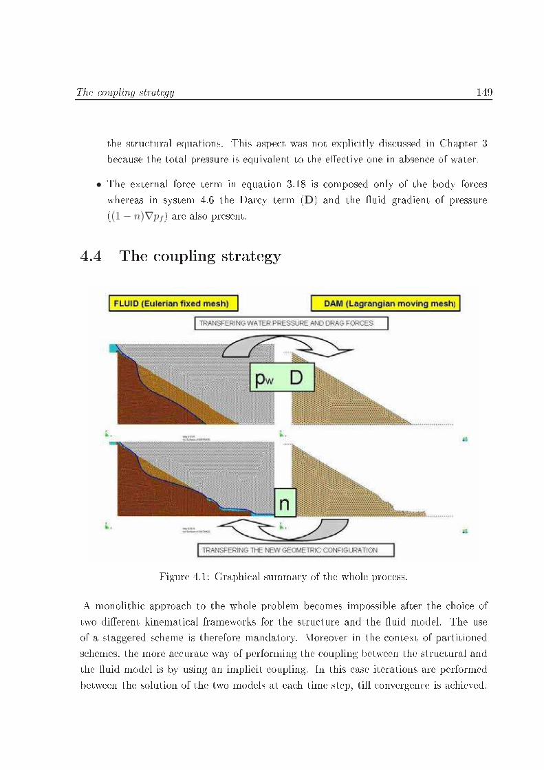
The oupling strategy 149the stru tural equations. This aspe t was not expli itly dis ussed in Chapter 3be ause the total pressure is equivalent to the ee tive one in absen e of water.• The external for e term in equation 3.18 is omposed only of the body for eswhereas in system 4.6 the Dar y term (D) and the uid gradient of pressure((1− n)∇pf) are also present.4.4 The oupling strategy

Figure 4.1: Graphi al summary of the whole pro ess.A monolithi approa h to the whole problem be omes impossible after the hoi e oftwo dierent kinemati al frameworks for the stru ture and the uid model. The useof a staggered s heme is therefore mandatory. Moreover in the ontext of partitioneds hemes, the more a urate way of performing the oupling between the stru tural andthe uid model is by using an impli it oupling. In this ase iterations are performedbetween the solution of the two models at ea h time step, till onvergen e is a hieved.

150 The ouplingThis hoi e is very a urate although very expensive. The se ond possibility, whi h isthe one used in the present work, is to perform an expli it oupling. This means thatthe solution at ea h time step is obtained by the solution of the uid and the stru turalmodel al ulated one after the other, without any iteration.This is a eptable onsidering that :• The adoption of a semi-expli it s heme for the uid problem leads to the need ofusing time steps mu h smaller than for the fully impli it stru tural problem, toensure stability. An impli it oupling would require adopting the smaller time step,i.e. that for the uid solver, for both models, leading to an extremely expensivepro edure;• The oupling between the two models is weaker in one of the two dire tions. Forthe solution of the uid problem, in fa t, only the porosity distribution is neededto be transfered by the stru tural model. In other words, the shape of the ro kllslope or, more generally, of the granular material have to be transfered to thexed uid mesh. On the ontrary the other way oupling, the uid pressure andvelo ity are essential to orre tly dene the external for es a ting on the ro kllmaterial.In summary the stru tural Lagrangian model is proje ted on the Eulerian xed meshdomain where, at the beginning of the simulation, the only available information is thein oming dis harge of water and the ontrol domain. The idea is that the uid analy-sis step is evaluated on e the distribution of porosity is proje ted from the stru turaldomain. The solution of the uid problem is then proje ted on the Lagrangian stru -tural mesh. It is ne essary to know the uid pressure and the Dar y for es in orderto evaluate orre tly the external for e term of the momentum equation in 4.6. On ethis is done, the stru tural response an be al ulated. Therefore, the granular domaindeforms a ordingly to the obtained velo ity and pressure elds. This new deformedgranular domain is nally proje ted onto the Eulerian mesh in order to solve for thesubsequent time step.Remark 20. The time step of the uid model is typi ally one order of magnitudesmaller than the one of the stru tural model. This is the onsequen e of the alreadydis ussed onditional stability of the semi-expli it s heme used for the uid model.Therefore the uid and the stru tural models have dierent time steps.

The oupling strategy 151The main points of the entire simulation pro ess are shown in Figure 4.1 and the ow hart of the algorithm are s hemati ally summarized in the box below:Coupling algorithmAssuming known the solution of the oupled problem at time step tn.1. Proje t the onguration of the ro kll material in terms of POROSITYdistribution on the Eulerian uid domain;2. SOLVE the water free surfa e ow problem al ulating the VELOCITYand PRESSURE eld in an EULERIAN xed mesh using the model pre-sented in Chapter 2;3. Proje t the FLUID VELOCITY and PRESSURE elds on the La-grangian stru tural mesh;4. Proje t the non linear DARCY TERM on the Lagrangian stru turalmesh;5. CALCULATE the stru tural response in a Lagrangian mesh, usingPFEM;6. Go ba k to step 1.4.4.1 Numeri al Example: Still water tank

Figure 4.2: Geometry of the tank and height of the ontained porous medium.The aim of this very simple example is to he k the al ulation of the ee tive pressuredistribution when no velo ity is present. A tank of porous material with three dierent

152 The oupling0.25m(a) Case 1 (hfA = 0.25m). 0.5m(b) Case 2 (hfB = 0.50m). ( ) Case 3 (hfC = 0.75m).Figure 4.3: Depth of water in the three analyzed ases.levels of water is analyzed. The geometry of the model an be seen in Figure 4.2 andthe three analyzed ases are shown in Figure 4.3. The hara teristi s of the materialare summed up in Table4.1. In the present example gravity is assumed to be 10m/s2.ROCKFILLGlobal density ρC = 1895.2 kg/m3Dry density ρs = 1490 kg/m3Porosity n = 0.4052Average diameter D50 = 35.04 mmWATERFluid density ρ = 1000.0 kg/m3Vis osity µ = 0.001 Pa sTable 4.1: Chara teristi s of the materials onsidered in the model.Let us dene:- hs: the depth of the porous medium (0.5m in the three ases);- hf : the water depth (hfA = 0.25m, hfB = 0.50m, hfC = 0.75m);- hw: the wet part of hs (hwA = 0.25m, hwB = 0.50m, hwC = 0.50m );- hd: the dry part of hs (hdA = 0.25m, hdB = 0.0m, hdC = 0.0m);- hfr

f : the water olumn over the porous medium (hfrA = 0.0m, hfrB = 0.0m,hfrC = 0.25m );The total bottom pressure (ps) in ea h ase an be al ulated analyti ally like the sumof the pressure of the wet part, the pressure of the dry part and the pressure of the

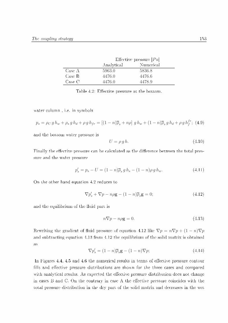
The oupling strategy 153Ee tive pressure [PaAnalyti al Numeri alCase A 5963.0 5836.8Case B 4476.0 4476.6Case C 4476.0 4478.9Table 4.2: Ee tive pressure at the bottom.water olumn , i.e. in symbolsps = ρC g hw + ρs g hd + ρ g hfr = [(1− n)ρs + nρ] g hw + (1− n)ρs g hd + ρ g hfr

f ; (4.9)and the bottom water pressure isU = ρ g h. (4.10)Finally the ee tive pressure an be al ulated as the dieren e between the total pres-sure and the water pressure

p′s = ps − U = (1− n)ρs g hs − (1− n)ρ g hw. (4.11)On the other hand equation 4.2 redu es to∇p′s +∇p− nρg − (1− n)ρsg = 0; (4.12)and the equilibrium of the uid part is

n∇p− nρg = 0. (4.13)Rewriting the gradient of uid pressure of equation 4.12 like ∇p = n∇p + (1 − n)∇pand subtra ting equation 4.13 from 4.12 the equilibrium of the solid matrix is obtainedas∇p′s = (1− n)ρsg− (1− n)∇p; (4.14)In Figures 4.4, 4.5 and 4.6 the numeri al results in terms of ee tive pressure ontourlls and ee tive pressure distributions are shown for the three ases and omparedwith analyti al results. As expe ted the ee tive pressure distribution does not hangein ases B and C. On the ontrary in ase A the ee tive pressure oin ides with thetotal pressure distribution in the dry part of the solid matrix and de reases in the wet

154 The oupling

(a) Contour ll of pressure. 0 1000 2000 3000 4000 5000 6000 7000PRESSURE[Pa]

0.0

0.2

0.4

0.6

0.8

1.0

WAT

ER L

EVEL

[m]

Low water level hfA=0.25m

Num Effective StressTheor Effective StressTheor Water PressureWater level

(b) Analyti al and numeri al results.Figure 4.4: Case A. hfA = 0.25m Ee tive Pressure p′

s.

(a) Contour ll of pressure. 0 1000 2000 3000 4000 5000 6000 7000PRESSURE[Pa]

0.0

0.2

0.4

0.6

0.8

1.0

WAT

ER L

EVEL

[m]

Medium water level hfB=0.50m

Num Effective StressTheor Effective StressTheor Water PressureWater level

(b) Analyti al and numeri al results.Figure 4.5: Case B. hfB = 0.50m Ee tive Pressure p′

s.

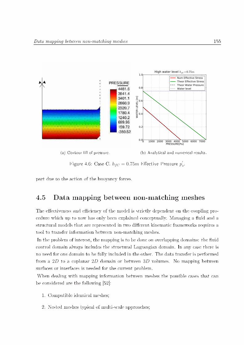
Data mapping between non-mat hing meshes 155

(a) Contour ll of pressure. 0 1000 2000 3000 4000 5000 6000 7000PRESSURE[Pa]

0.0

0.2

0.4

0.6

0.8

1.0

WAT

ER L

EVEL

[m]

High water level hfC=0.75m

Num Effective StressTheor Effective StressTheor Water PressureWater level

(b) Analyti al and numeri al results.Figure 4.6: Case C. hfC = 0.75m Ee tive Pressure p′

s.part due to the a tion of the buoyan y for es.4.5 Data mapping between non-mat hing meshesThe ee tiveness and e ien y of the model is stri tly dependent on the oupling pro- edure whi h up to now has only been explained on eptually. Managing a uid and astru tural models that are represented in two dierent kinemati frameworks requires atool to transfer information between non-mat hing meshes.In the problem of interest, the mapping is to be done on overlapping domains: the uid ontrol domain always in ludes the stru tural Lagrangian domain. In any ase there isno need for one domain to be fully in luded in the other. The data transfer is performedfrom a 2D to a oplanar 2D domain or between 3D volumes. No mapping betweensurfa es or interfa es is needed for the urrent problem.When dealing with mapping information between meshes the possible ases that anbe onsidered are the following [52:1. Compatible identi al meshes;2. Nested meshes typi al of multi-s ale approa hes;

156 The oupling3. Non-nested meshes with a large dieren e between their sizes, typi al of aeronauti problems;4. Dissimilar meshes in general.In the present work the need of mapping from a moving to a xed mesh and vi e-versaleads to dis ard the rst two groups. On the other hand, there is no parti ular reasonwhy the order of magnitude of the two meshes should dier very mu h. Therefore the ase of interest is the 4th one. Also the uid and the stru tural problems do not haveany Gauss point variable to be mapped. This simplies the problem that redu es to thetransfer between nodal variables of non-mat hing meshes.Let us dene origin mesh (OM) the mesh from whi h the variable α is to be transferedto the destination mesh (DM). In this framework, a ording to [18 the transfer methods an be lassied as follow:1. The Element Transfer Method (ETM). For ea h node of the DM a sear h is per-formed in order to lo ate the element of the OM it is in luded in. The value of αis obtained by interpolating the nodal values of su h element.2. The Mortar Element Transfer Method (METM) in whi h onservation of the eldsis imposed in a weak sense. The dieren e between the value of the eld on theDM and its value on the OM is asked to be zero weakly performing an integrationon the DM [52.3. The Finite Volume Transfer Method (FVTM) where the onservation in a weaksense is obtained using the Finite Volume Method [102.4. The Conve tion Transfer Method (CVM) whi h is a modi ation of the previousalgorithm suitable for Arbitrary Lagrangian Eulerian methods in whi h neitherthe number of nodes, nor the onne tivity hange during the al ulation [18.The ETM is a dissipative pro edure that might reate a serious data loss if the dimensionof the two meshes is very dierent. Nevertheless, due to its simpli ity and onsideringthe weak oupling of the physi al simulated phenomenon , it is the method hosen inthis work.Let us refer to Figure 4.7 to explain the ETM algorithm. The data transfer an beperformed via the following steps. For every element (ABC) of the OM:

Data mapping between non-mat hing meshes 157

DESTINATION MESH

ORIGIN MESH

A

B

C

I

JK

Figure 4.7: 2D example of the interpolation pro edure. Node I, J and K are inside the ir ums ribed ir le but only node J in inside the element and its value of alpha an be al ulated.1. Cal ulate the sphere that ir ums ribes the element, or ir le in 2D (bla k ir lein Figure 4.7);2. Sear h all the nodes of the DM inside the sphere (nodes I, J and K in Figure 4.7);3. Che k whi h of them is inside the element (verifying that the value of the shapefun tions of the element nodes are all positive and smaller than one);0 < NA(xJ) < 1; (4.15)0 < NB(xJ) < 1; (4.16)0 < NC(xJ) < 1; (4.17)4. For every destination node inside the element of the OM (node J of Figure 4.7),interpolate the value of α

αJ = NA(xJ)αA +NB(xJ)αB +NC(xJ)αC ;Remark 21. The variable α an be either a s alar or a ve tor. A third possibility isleft to the user: he/she an hoose to map the whole origin model on the destinationone.In order to perform step 2 the use of a spatial sear h data stru ture is needed. The

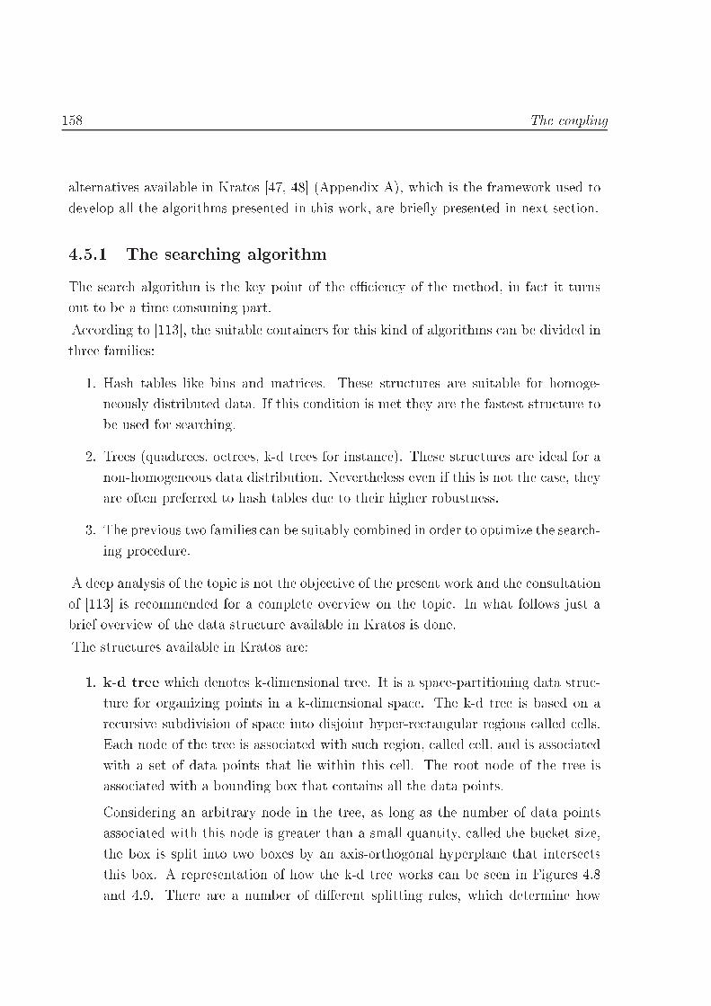
158 The ouplingalternatives available in Kratos [47, 48 (Appendix A), whi h is the framework used todevelop all the algorithms presented in this work, are briey presented in next se tion.4.5.1 The sear hing algorithmThe sear h algorithm is the key point of the e ien y of the method, in fa t it turnsout to be a time onsuming part.A ording to [113, the suitable ontainers for this kind of algorithms an be divided inthree families:1. Hash tables like bins and matri es. These stru tures are suitable for homoge-neously distributed data. If this ondition is met they are the fastest stru ture tobe used for sear hing.2. Trees (quadtrees, o trees, k-d trees for instan e). These stru tures are ideal for anon-homogeneous data distribution. Nevertheless even if this is not the ase, theyare often preferred to hash tables due to their higher robustness.3. The previous two families an be suitably ombined in order to optimize the sear h-ing pro edure.A deep analysis of the topi is not the obje tive of the present work and the onsultationof [113 is re ommended for a omplete overview on the topi . In what follows just abrief overview of the data stru ture available in Kratos is done.The stru tures available in Kratos are:1. k-d tree whi h denotes k-dimensional tree. It is a spa e-partitioning data stru -ture for organizing points in a k-dimensional spa e. The k-d tree is based on are ursive subdivision of spa e into disjoint hyper-re tangular regions alled ells.Ea h node of the tree is asso iated with su h region, alled ell, and is asso iatedwith a set of data points that lie within this ell. The root node of the tree isasso iated with a bounding box that ontains all the data points.Considering an arbitrary node in the tree, as long as the number of data pointsasso iated with this node is greater than a small quantity, alled the bu ket size,the box is split into two boxes by an axis-orthogonal hyperplane that interse tsthis box. A representation of how the k-d tree works an be seen in Figures 4.8and 4.9. There are a number of dierent splitting rules, whi h determine how

Data mapping between non-mat hing meshes 159

Figure 4.8: S hemati representation of a k-d tree data stru ture taken from [69.

Figure 4.9: Representation of a k-d tree partitioning taken from [47.this hyperplane is sele ted and hara terize the k-d tree. In Kratos the availableoptions are the following:a) Mid splitting rule. The ell is always divided by half;b) Balan ed splitting rule. The ell is divided into two ells that ontain thesame number of nodes. This is an optimal rule but very time onsuming; ) Approximated balan ed rule. It uses the average of the oordinates of thepoints as splitting dimension.2. Bins It divides the domain into a regular nx× ny × nz sub-domains as shown inFigure 4.10 and holds an array of bu kets storing its elements (see Figure 4.11).

160 The ouplingThis stru ture provides an extremely fast spatial sear hing when entities are moreor less uniformly distributed over the domain. The good performan e for welldistributed entities and their simpli ity makes bins one of the most popular datastru ture for dierent nite element appli ations.Figure 4.10: Representation of a bins partitioning taken from [47.

Figure 4.11: Bins stru ture taken from [47.Two bins stru tures are implemented in Kartos:a) Stati bins. This is the most e ient bins stru ture organizing the data insparse matri es but does not allow the insertion of additional data.b) Dynami bins. Slower than the previous one, it is basi ally a matrix of arraysof entries, allowing a more exible modi ation of its ontent at any time.3. O tree. It is a type of tree in whi h every node in 3D has hildren. Spa eis re ursively subdivided into eight o tants (only o tants ontaining nodes aredivided in turn). The reation of the tree is faster than in th k-d tree ase but theresulting stru ture an often be less balan ed. The sear hing pro edure is fasterthan in k-d tree implying less jumps.4. K-d tree of bins a ombination of the previous des ribed stru tures.

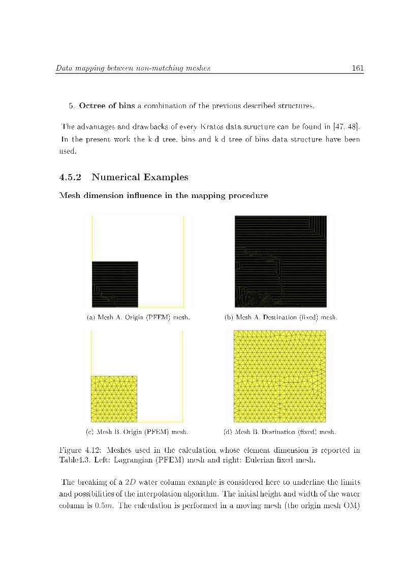
Data mapping between non-mat hing meshes 1615. O tree of bins a ombination of the previous des ribed stru tures.The advantages and drawba ks of every Kratos data stru ture an be found in [47, 48.In the present work the k-d tree, bins and k-d tree of bins data stru ture have beenused.4.5.2 Numeri al ExamplesMesh dimension inuen e in the mapping pro edure

(a) Mesh A. Origin (PFEM) mesh. (b) Mesh A. Destination (xed) mesh.

( ) Mesh B. Origin (PFEM) mesh. (d) Mesh B. Destination (xed) mesh.Figure 4.12: Meshes used in the al ulation whose element dimension is reported inTable4.3. Left: Lagrangian (PFEM) mesh and right: Eulerian xed mesh.The breaking of a 2D water olumn example is onsidered here to underline the limitsand possibilities of the interpolation algorithm. The initial height and width of the water olumn is 0.5m. The al ulation is performed in a moving mesh (the origin mesh OM)

162 The ouplingusing PFEM, and at ea h time step the whole model part is proje ted to the xed mesh(the destination mesh DM). A k-d tree data stru ture is used to perform the sear hingof the neighbors. Mesh A Mesh BDimension [m 0.005 0.05Table 4.3: Size of the two meshes onsidered in the proje tion example.Two dierent mesh sizes are onsidered for the interpolation pro edure, a ne mesh(mesh A of Table4.3) with approximately 100 elements in the water olumn edge and a oarser one (Mesh B of Table 4.3) with 10. The Eulerian and Lagrangian initial domainsfor the two meshes onsidered are shown in Figure 4.12. In Figure 4.13 the interpola-tion is performed from mesh A to a xed grid with the same mesh dimension. Wheninterpolating data between oarser PFEM and xed meshes (mesh B) the interpolationshows a la k of pre ision (gure 4.14). Nevertheless it should be observed that originaldata are already quite poor and no relevant data loss is present.The worst performan e is observed when interpolating form a PFEM model with meshA to a oarse xed mesh (mesh B). The loss of information is evident in Figure 4.15.Therefore as a on lusion, the dimension of the origin and destination meshes has to beof the same order of magnitude to obtain an a eptable pre ision in the interpolationpro edure.Performing the proje tion algorithmIn the present example the time performan e of the interpolation algorithm is al ulatedfor a k-d tree, bins and k-d tree of bins data stru tures. The example onsiders theproje tion of a s alar variable (the porosity) from a PFEM model to a xed grid model.The meshes are unstru tured and homogeneous. The same dimension is onsidered inthe Lagrangian and Eulerian models.Four dierent meshes are onsidered for the omparison. The detail of ea h of them anbe found in Table4.4. The results are summarized in Figure 4.16 where, as expe ted,in the ase of an homogeneous mesh, the bins stru ture is mu h faster than the k-dtree one. The dieren e is learer as mu h as the mesh is rened. Nevertheless the

Data mapping between non-mat hing meshes 163

(a) Origin (PFEM) mesh (b) Destination (xed) mesh. ( )Figure 4.13: Mapping between models with Mesh A.

(a) Origin (PFEM) mesh (b) Destination (xed) mesh. ( )Figure 4.14: Mapping between models with Mesh B.

164 The oupling

(a) Origin (PFEM) mesh (b) Destination (xed) mesh. ( )Figure 4.15: Mapping from a ne mesh (mesh A) to a oarse one (mesh B). ombination of these two stru tures resulting in a k-d tree of bins improve relevantlythe e ien y of the simple k-d tree.The e ien y of the bins an be ompromised for a mesh with very high dieren e inthe dimension. In that ase, the splitting rule of the k-d tree is the faster sear hingpro edure [113.Con erning the problem of interest of the present work, the results onrm that thereis no reason why the mesh should vary very mu h in the ase of the oupled models ofro kll dams that will be presented in next hapter.Mesh A Mesh B Mesh C Mesh DDimension [m 0.02 0.03 0.04 0.05Eul Lagr Eul Lagr Eul Lagr Eul Lagrn. nodes 8 200 2 600 3 600 1 200 2 000 700 3 700 460n. elem 15 900 7 400 7 000 3 300 4 000 1 800 7 000 1 200Table 4.4: Mesh dimension of the four meshes onsidered in the proje tion example. Thelast two rows indi ates the number of nodes and elements for the Eulerian destinationmesh (Eul) and the Lagrangian origin one (Lagr).

Con lusions 165

0.020 0.025 0.030 0.035 0.040 0.045 0.050MESH SIZE [m]

0.00

0.01

0.02

0.03

0.04

0.05

TIM

E FO

R IN

TERP

OLA

TIO

N [s

]

K-D TREEBINSK-D TREE OF BINS

Figure 4.16: Comparison between the performan e of k-d tree, bins, and k-d tree of binsdata stru tures for the proje tion of a s alar variable for dierent mesh sizes.4.6 Con lusionsIn the present hapter the staggered balan e equations of the oupled model have beenderived from the global balan e equations. The expli it oupling strategy is des ribedand a simple example has been used to he k the apability of the model of al ulatingthe ee tive pressure distribution for a stati ase.In the se ond part of the hapter a pro edure to map variables from non-mat hingmeshes is presented. After a brief overview of the possible data passing models theimplemented Element Transfer Method is explained. In spite of the diusivity of themethod and its moderate a ura y, it is hosen be ause of its simpli ity. In the futurethis tool ould be easily substituted with a more e ient proje tion te hnique. Thesear hing algorithms available in Kratos have been presented.The examples analyzed lead to the following on lusions:1. The origin and the destination mesh should be of the same order of magnitude toensure an a urate data mapping.2. The stati bins stru ture is the best hoi e for an homogeneous distribution of the

166 The ouplingnodes, Nevertheless the k-d tree data stru ture an be ompetitive for exampleswith an alternation of dense and sparse distribution of nodes.In any ase a deeper study on the performan e of the mapping te hnique is to be donein order to optimize the ode.

Chapter 5Failure analysis of s ale models ofro kll dams under seepage onditionsIn the present hapter the seepage and the oupled models are validated through a omparison with the experimental results on s ale models of ro kll dams in dierentseepage onditions, arried out by UPM and CEDEX during the XPRES and E-DAMSproje ts [53, 127. The ee tiveness of the models are tested on 2D and 3D models ofro kll dams with dierent types of impermeabilization. The inuen e of some physi aland me hani al parameters is studied to alibrate the odes.5.1 Introdu tionThe extensive work of UPM and CEDEX during the XPRES and E-DAMS proje ts[53, 127 results in more than 100 experiments. Three experimental fa ilities of dierentdimensions have been used (they an be seen in Figure 1.6 of Chapter 1). The mainobje tive of the experimentalists during the XPRES proje t was the analysis of theinuen e of a series of parameters and of their ombination, on the failure me hanismof the dam.The experimental ampaign investigated the ee t of• the type of impermeabilization;• the slope of the downstream part;• the dimension of the material used;

168 Failure analysis of s ale models of ro kll dams under seepage onditions• the randomness in the experiments;• the in oming dis harge1;• the s ale ee t;Ea h experiment studies a s ale model dam under a series of in remental steps ofdis harge. After ea h in rement, the in oming dis harge is maintained onstant tillrea hing the steady state. When a brea h appears in the downstream slope, its stabi-lization is a hieved before measuring its advan e.Pressure heads is registered and the length of failure is therefore measured at ea hstep.

(a) Front view of UPM hannel withthe pressure sensors tubes. (b) One of the panels for readingpressure heights.Figure 5.1: Pressure instrumentation.Pressure at the bottom of the umes is evaluated by a network of sensors Figure 5.1(a).Its value is read on millimetri panels like the one shown in Figure 5.1(b).The deformation of the dam is analyzed through the evolution of the so alled lengthof failure (B parameter in Figure 5.2(a)). It is, by denition, the horizontal proje tionof the distan e between the initial undeformed downstream toe and the higher point ofthe failed area.Usually olored horizontal strikes are painted on the initial slope. This helps the mea-surement of B (see Figure 5.2(b) for instan e). In some of the experiments a moredetailed measurement of the evolution of failure is performed using a lose-obje t-photogrammetry-te hnique. It onsists on taking a series of photos with a very short1The in oming dis harge is a boundary ondition of the experiment. It is the dis harge (in l/s)pumped upstream by the laboratory pumps.

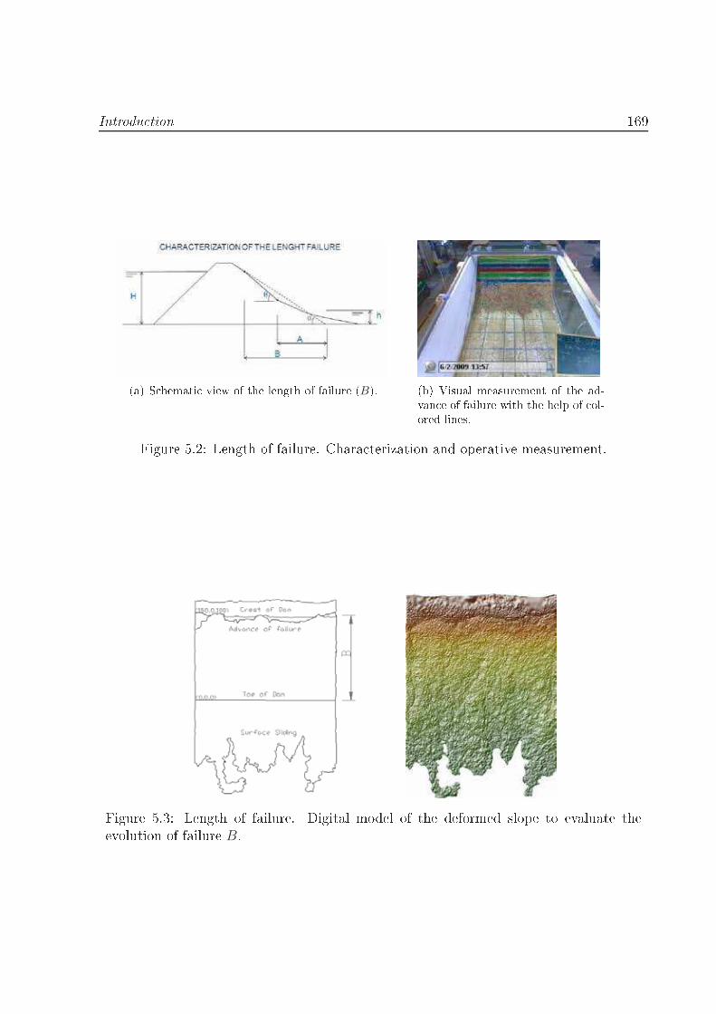
Introdu tion 169

(a) S hemati view of the length of failure (B). (b) Visual measurement of the ad-van e of failure with the help of ol-ored lines.Figure 5.2: Length of failure. Chara terization and operative measurement.

Figure 5.3: Length of failure. Digital model of the deformed slope to evaluate theevolution of failure B.

170 Failure analysis of s ale models of ro kll dams under seepage onditionstime interval until the end of the simulation. Through the re-elaboration of this data,the reation of a digital model of the deformed dam is possible and the dynami evolutionof the brea h is followed with high pre ision (see for instan e Figure 5.3).The experiment ends when failure rea hes the rest of the dam.The analysis of the experimental ampaign is not the obje tive of the present work andfor more details on the topi , the onsultation of [21, 76 is re ommended. Neverthelesssome important on lusions of the experimental study are summarized here in order tomotivate the hoi e of the ase study presented in the following se tions.1. As explained in Chapter 1, there exists two main failure me hanisms in a ro kllslope when overtopping o urs: mass sliding and dragging of parti les. They a tin ombined or alternative way prin ipally depending on the geometri al hara -teristi s of the downstream slope. For steep slopes (1.5H : 1V for instan e) masssliding predominates over dragging of parti les. The opposite o urs when theslope is very at (3H : 1V for instan e). Taking into a ount this important as-pe t, UPM and CEDEX observed that data-s atter is higher in the experimentswith intermediate slopes, where neither the mass sliding nor the erosion arepredominant but their a tion is ombined.2. The length of failure of the rst steps of dis harge (that is for low water level),presents a rather high data s atter on erning the evolution of the brea h. Onthe ontrary the dis harge for whi h failure rea hes the rest is always in greata ordan e.3. No lear relation an be found between the unit failure dis harge2 and the down-stream slope.4. Considering prototype dams of the same dimension, it has been observed that fora ore dam, the unit failure dis harge is between 10 and 20% lower than for otherkind of dams.5. The unit failure dis harge in reased for material with higher D50.6. Failure is observed to be more fragile in the ase of steepest slopes for whi h thepredominant failure me hanism is mass sliding.2The unit failure dis harge is the dis harge for unit length of the ume, for whi h the failure rea hesthe rest of the prototype dam.

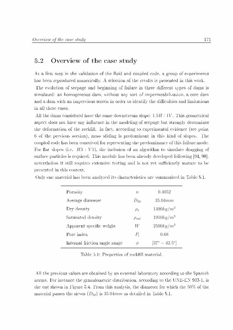
Overview of the ase study 1715.2 Overview of the ase studyAs a rst step in the validation of the uid and oupled ode, a group of experimentshas been reprodu ed numeri ally. A sele tion of the results is presented in this work.The evolution of seepage and beginning of failure in three dierent types of dams issimulated: an homogeneous dam, without any sort of impermeabilization, a ore damand a dam with an impervious s reen in order to identify the di ulties and limitationsin all these ases.All the dams onsidered have the same downstream slope: 1.5H : 1V . This geometri alaspe t does not have any inuen e in the modeling of seepage but strongly determinesthe deformation of the ro kll. In fa t, a ording to experimental eviden e (see point6 of the previous se tion), mass sliding is predominant in this kind of slopes. The oupled ode has been on eived for representing the predominan e of this failure mode.For at slopes (i.e. H3 : V 1), the in lusion of an algorithm to simulate dragging ofsurfa e parti les is required. This module has been already developed following [94, 98,nevertheless it still requires extensive testing and is not yet su iently mature to bepresented in this ontext.Only one material has been analyzed its hara teristi s are summarized in Table 5.1.Porosity n 0.4052Average diameter D50 35.04mmDry density ρs 1490kg/m3Saturated density ρsat 1910kg/m3Apparent spe i weight W 2500kg/m3Pore index Pi 0.68Internal fri tion angle range φ [37 − 42.5]Table 5.1: Properties of ro kll material.All the previous values are obtained by an external laboratory a ording to the Spanishnorms. For instan e the granulometri distribution, a ording to the UNE-EN 933-1, isthe one shown in Figure 5.4. From this analysis, the diameter for whi h the 50% of thematerial passes the sieves (D50) is 35.04mm as detailed in Table 5.1.

172 Failure analysis of s ale models of ro kll dams under seepage onditions

Figure 5.4: Granulometri analysis of ro kll material a ording to the UNE-EN 933-1.This is the largest material used in the experimental ampaign. A dire t relation be-tween the dimension of the grains and the dis harge of beginning of failure was observed.This implies the possibility of working with higher velo ities. In fa t this represents apositive aspe t be ause the level set te hnique an present some problems with very lowvelo ities (i.e. very low water depth). Just to make an example, at the beginning of thesimulation the Froude number3 an be of the order of 10−2.Finally for ea h experiment, dierent steps of dis harge have been simulated. In allthe ases with the lower dis harge onsidered no movements in the downstream slope isobserved. This implies that, in order to speed up the al ulations, the uid un oupled ode an be used for the simulation. The oupled model is used for the higher dis harges.Before presenting of the results, the nomen lature used to lassify the ases is brieyresumed here.Three dierent type of dams are simulated in the present hapter:- CASE A: an homogeneous dam without impermeabilization.3Froude number is an a-dimensional number indi ating the ratio between gravity and inertia for es.It is used to lassify the ow regime [58.

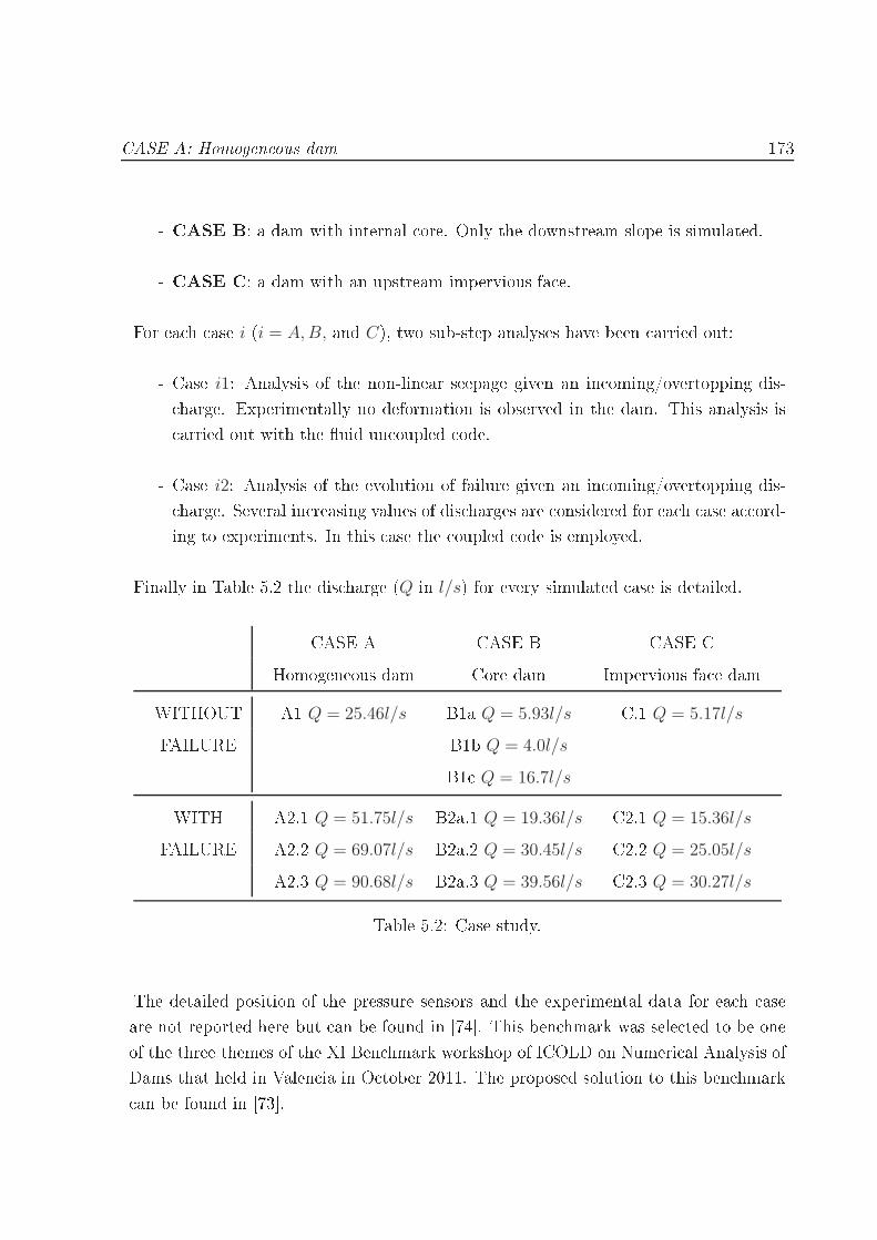
CASE A: Homogeneous dam 173- CASE B: a dam with internal ore. Only the downstream slope is simulated.- CASE C: a dam with an upstream impervious fa e.For ea h ase i (i = A,B, and C), two sub-step analyses have been arried out:- Case i1: Analysis of the non-linear seepage given an in oming/overtopping dis- harge. Experimentally no deformation is observed in the dam. This analysis is arried out with the uid un oupled ode.- Case i2: Analysis of the evolution of failure given an in oming/overtopping dis- harge. Several in reasing values of dis harges are onsidered for ea h ase a ord-ing to experiments. In this ase the oupled ode is employed.Finally in Table 5.2 the dis harge (Q in l/s) for every simulated ase is detailed.CASE A CASE B CASE CHomogeneous dam Core dam Impervious fa e damWITHOUT A1 Q = 25.46l/s B1a Q = 5.93l/s C.1 Q = 5.17l/sFAILURE B1b Q = 4.0l/sB1 Q = 16.7l/sWITH A2.1 Q = 51.75l/s B2a.1 Q = 19.36l/s C2.1 Q = 15.36l/sFAILURE A2.2 Q = 69.07l/s B2a.2 Q = 30.45l/s C2.2 Q = 25.05l/sA2.3 Q = 90.68l/s B2a.3 Q = 39.56l/s C2.3 Q = 30.27l/sTable 5.2: Case study.The detailed position of the pressure sensors and the experimental data for ea h aseare not reported here but an be found in [74. This ben hmark was sele ted to be oneof the three themes of the XI Ben hmark workshop of ICOLD on Numeri al Analysis ofDams that held in Valen ia in O tober 2011. The proposed solution to this ben hmark an be found in [73.

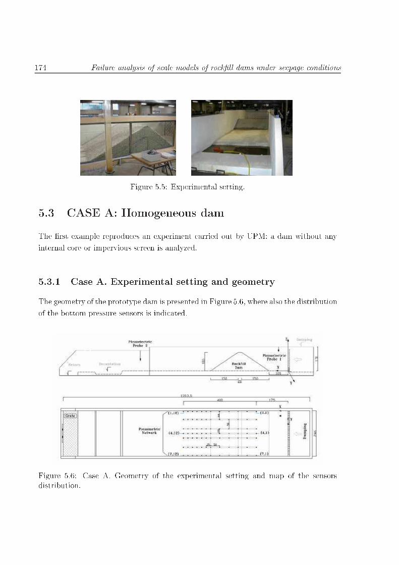
174 Failure analysis of s ale models of ro kll dams under seepage onditions

Figure 5.5: Experimental setting.5.3 CASE A: Homogeneous damThe rst example reprodu es an experiment arried out by UPM: a dam without anyinternal ore or impervious s reen is analyzed.5.3.1 Case A. Experimental setting and geometryThe geometry of the prototype dam is presented in Figure 5.6, where also the distributionof the bottom pressure sensors is indi ated.

Figure 5.6: Case A. Geometry of the experimental setting and map of the sensorsdistribution.

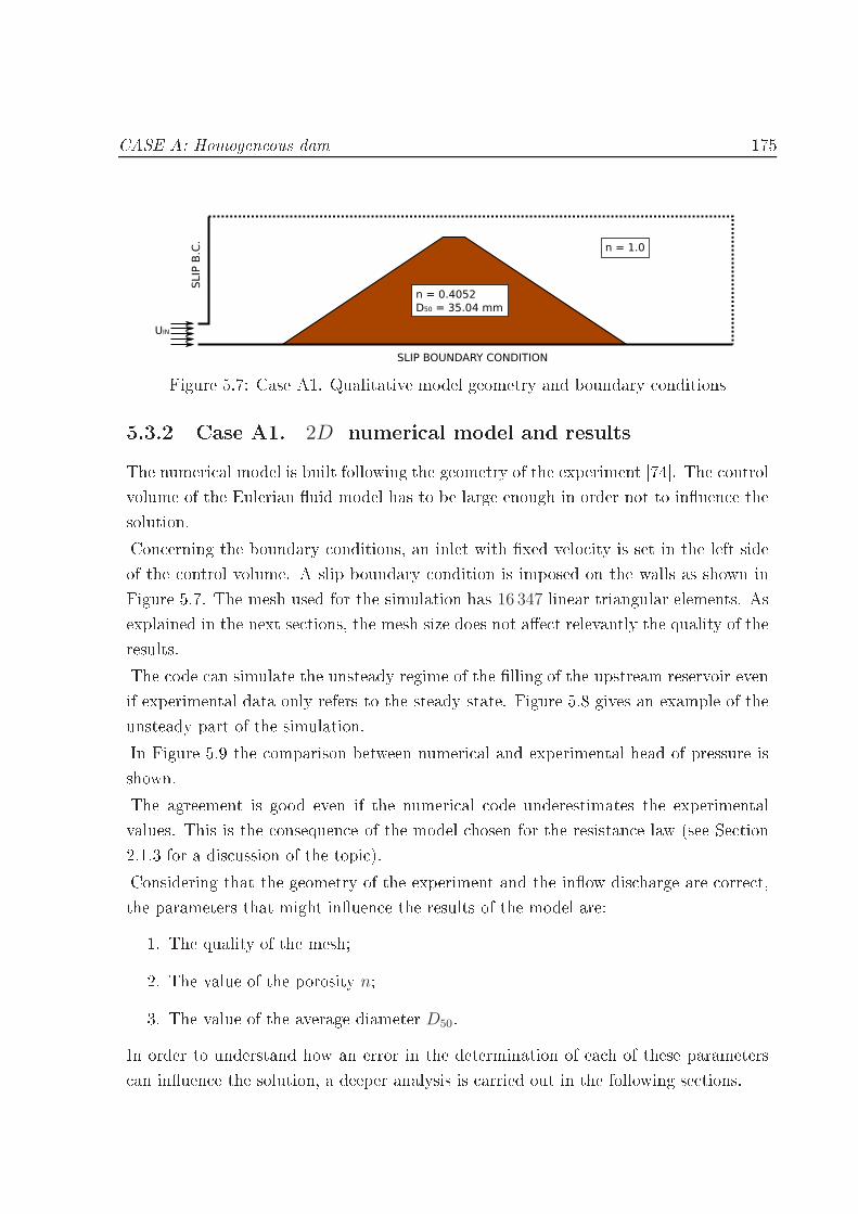
CASE A: Homogeneous dam 175n = 0.4052

D50 = 35.04 mm

n = 1.0

UIN

SLIP BOUNDARY CONDITION

SLIP

B.C

.

Figure 5.7: Case A1. Qualitative model geometry and boundary onditions5.3.2 Case A1. 2D numeri al model and resultsThe numeri al model is built following the geometry of the experiment [74. The ontrolvolume of the Eulerian uid model has to be large enough in order not to inuen e thesolution.Con erning the boundary onditions, an inlet with xed velo ity is set in the left sideof the ontrol volume. A slip boundary ondition is imposed on the walls as shown inFigure 5.7. The mesh used for the simulation has 16 347 linear triangular elements. Asexplained in the next se tions, the mesh size does not ae t relevantly the quality of theresults.The ode an simulate the unsteady regime of the lling of the upstream reservoir evenif experimental data only refers to the steady state. Figure 5.8 gives an example of theunsteady part of the simulation.In Figure 5.9 the omparison between numeri al and experimental head of pressure isshown.The agreement is good even if the numeri al ode underestimates the experimentalvalues. This is the onsequen e of the model hosen for the resistan e law (see Se tion2.1.3 for a dis ussion of the topi ).Considering that the geometry of the experiment and the inow dis harge are orre t,the parameters that might inuen e the results of the model are:1. The quality of the mesh;2. The value of the porosity n;3. The value of the average diameter D50.In order to understand how an error in the determination of ea h of these parameters an inuen e the solution, a deeper analysis is arried out in the following se tions.

176 Failure analysis of s ale models of ro kll dams under seepage onditions

Figure 5.8: Case A1. Evolution of the seepage line in a dam with porosity n = 0.4 andD50 = 35mm. Q = 25, 46l/s.

0.0 0.5 1.0 1.5 2.0 2.5 3.0 3.5[m]

0.0

0.2

0.4

0.6

0.8

1.0

PRES

SURE

[m]

Q=25.46l/sDam shapeNumerical resultsExp results

Figure 5.9: Case A1. Bottom pressure distribution at stationary regime for Q =25, 46l/s. Porosity n = 0.4, D50 = 35mm. Numeri al and experimental omparison.

CASE A: Homogeneous dam 1775.3.3 Case A1. Mesh inuen eIn order to understand how the mesh inuen es the results, ase A1 is run with dierentmeshes. The inlet area has been left onstantly rened (href = 0.01m4) in order to ensurea onstant in oming dis harge before entering the porous medium. The hara teristi sof the meshes are summarized in Table 5.3 and an be seen in Figures 5.10.Mesh A Mesh B Mesh C Mesh DDimension [m 0.01 0.1 0.15 0.20n. elem 43 500 550 310 220n. nodes 86 100 970 510 340Table 5.3: Case A1. Mesh sizes used in the mesh sensitivity study.Results shows that the mesh does not seem to have a strong inuen e on the quality ofthe results at least inside the dam when no impervious stru tures are present. The maindieren e an be observed at the downstream toe of the dam, where water omes out ofthe granular material. For oarser meshes an important loss of volume an be observedoutside the ro kll. The presen e of the porous medium with its dissipative ee t ishelpful in enfor ing the volume onservation properties also for very oarse meshes likemesh D, for instan e. This is no longer true outside the granular material.This aspe t should be taken into a ount when hoosing the mesh for a simulation.5.3.4 Case A1. Inuen e of porosityThe porosity of the material used in the experiments presented in this hapter is evalu-ated by an external laboratory a ording to the Spanish norm UNE-EN 1936:2007 andis 0.4052.Keeping all the parameters of the models and the al ulation mesh xed, porosity is hanged in the range 0.30 − 0.45 in order to see the inuen e of this parameter in theanalysis. A onstant variation in the porosity value ∆n indu es a onstant jump in thepressure head distribution as an be observed in Figure 5.12.4h is the average mesh dimension. In this ase the sub-index ref indi ates that this h refers to therened areas at the inlet.

178 Failure analysis of s ale models of ro kll dams under seepage onditions(a) Mesh A (b) Mesh B( ) Mesh C (d) Mesh DFigure 5.10: Case A1. Meshes used in the analysis of mesh sensitivity. Detailed hara -teristi s of the meshes an be found in Table 5.3.

0.0 0.5 1.0 1.5 2.0 2.5 3.0 3.5[m]

0.0

0.2

0.4

0.6

0.8

1.0

PRES

SURE

[m]

Mesh sensitivity testDam shapeExp. n=0.4052, D50=35.04mm

MeshA(0.01m)

MeshB(0.1m)

MeshC(0.15m)

MeshD(0.2m)

Figure 5.11: Case A1. Inuen e of the mesh.

0.0 0.5 1.0 1.5 2.0 2.5 3.0 3.5[m]

0.0

0.2

0.4

0.6

0.8

1.0

PRES

SURE

[m]

n sensitivity testDam shapeExp. n=0.4052

n=0.30m

n=0.35m

n=0.40m

n=0.45m

Figure 5.12: Case A1. Pressure head distribution for porosity n = 0.3, 0.35, 0.4 and0.45.

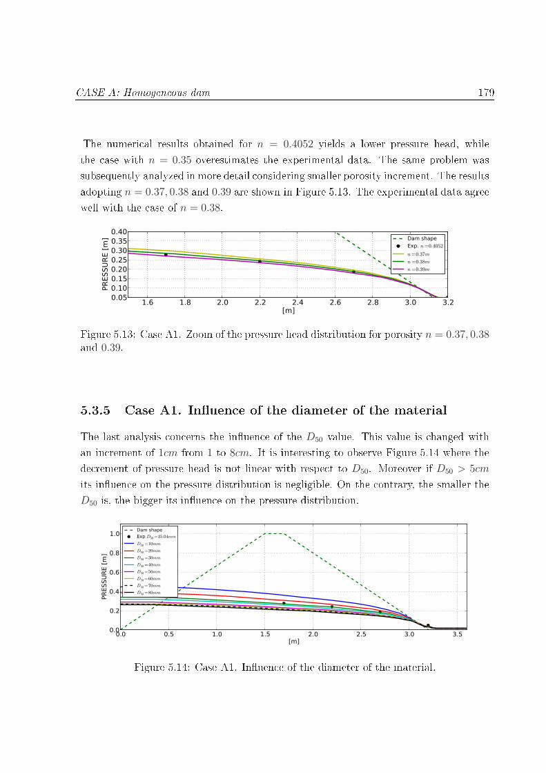
CASE A: Homogeneous dam 179The numeri al results obtained for n = 0.4052 yields a lower pressure head, whilethe ase with n = 0.35 overestimates the experimental data. The same problem wassubsequently analyzed in more detail onsidering smaller porosity in rement. The resultsadopting n = 0.37, 0.38 and 0.39 are shown in Figure 5.13. The experimental data agreewell with the ase of n = 0.38.1.6 1.8 2.0 2.2 2.4 2.6 2.8 3.0 3.2

[m]0.050.100.150.200.250.300.350.40

PRES

SURE

[m]

n sensitivity test zoomDam shapeExp. n=0.4052

n=0.37m

n=0.38m

n=0.39m

Figure 5.13: Case A1. Zoom of the pressure head distribution for porosity n = 0.37, 0.38and 0.39.5.3.5 Case A1. Inuen e of the diameter of the materialThe last analysis on erns the inuen e of the D50 value. This value is hanged withan in rement of 1cm from 1 to 8cm. It is interesting to observe Figure 5.14 where thede rement of pressure head is not linear with respe t to D50. Moreover if D50 > 5cmits inuen e on the pressure distribution is negligible. On the ontrary, the smaller theD50 is, the bigger its inuen e on the pressure distribution.

0.0 0.5 1.0 1.5 2.0 2.5 3.0 3.5[m]

0.0

0.2

0.4

0.6

0.8

1.0

PRES

SURE

[m]

D50 sensitivity testDam shapeExp D50=35.04mm

D50=10mm

D50=20mm

D50=30mm

D50=40mm

D50=50mm

D50=60mm

D50=70mm

D50=80mm

Figure 5.14: Case A1. Inuen e of the diameter of the material.

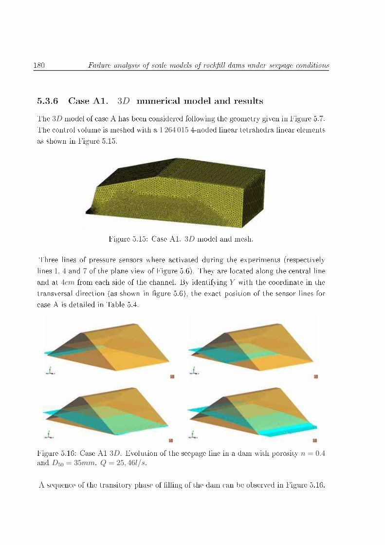
180 Failure analysis of s ale models of ro kll dams under seepage onditions5.3.6 Case A1. 3D numeri al model and resultsThe 3D model of ase A has been onsidered following the geometry given in Figure 5.7.The ontrol volume is meshed with a 1 264 015 4-noded linear tetrahedra linear elementsas shown in Figure 5.15.

Figure 5.15: Case A1. 3D model and mesh.Three lines of pressure sensors where a tivated during the experiments (respe tivelylines 1, 4 and 7 of the plane view of Figure 5.6). They are lo ated along the entral lineand at 4cm from ea h side of the hannel. By identifying Y with the oordinate in thetransversal dire tion (as shown in gure 5.6), the exa t position of the sensor lines for ase A is detailed in Table 5.4.

Figure 5.16: Case A1 3D. Evolution of the seepage line in a dam with porosity n = 0.4and D50 = 35mm. Q = 25, 46l/s.A sequen e of the transitory phase of lling of the dam an be observed in Figure 5.16.

CASE A: Homogeneous dam 181Line 1 at Y = 0.04mLine 4 at Y = 1.23mLine 7 at Y = 2.42mTable 5.4: A tivated sensors lines in ase A.

0.0 0.5 1.0 1.5 2.0 2.5 3.0 3.5[m]

0.0

0.2

0.4

0.6

0.8

1.0

PRES

SURE

[m]

Q=25.46l/s. Sensor line y = 0.04mDam shapeNumerical resultsExp results

0.0 0.5 1.0 1.5 2.0 2.5 3.0 3.5[m]

0.0

0.2

0.4

0.6

0.8

1.0

PRES

SURE

[m]

Q=25.46l/s. Sensor line y = 1.23mDam shapeNumerical resultsExp results

0.0 0.5 1.0 1.5 2.0 2.5 3.0 3.5[m]

0.0

0.2

0.4

0.6

0.8

1.0

PRES

SURE

[m]

Q=25.46l/s. Sensor line y = 2.42mDam shapeNumerical resultsExp results

Figure 5.17: Case A1 (3D). Bottom pressure distribution at stationary regime along thethree sensors lines (Y = 0.04m, 1.23m, 2.42m respe tively) for Q = 25, 46l/s. Porosityn = 0.4, D50 = 35mm. Numeri al and experimental omparison.

182 Failure analysis of s ale models of ro kll dams under seepage onditions

0.0 0.5 1.0 1.5 2.0 2.5 3.0 3.5[m]

0.0

0.2

0.4

0.6

0.8

1.0

PRES

SURE

[m]

Q=25.46l/s. Time 10s.Dam shape2d results3d results

0.0 0.5 1.0 1.5 2.0 2.5 3.0 3.5[m]

0.0

0.2

0.4

0.6

0.8

1.0

PRES

SURE

[m]

Q=25.46l/s. Time 25s.Dam shape2d results3d results

0.0 0.5 1.0 1.5 2.0 2.5 3.0 3.5[m]

0.0

0.2

0.4

0.6

0.8

1.0

PRES

SURE

[m]

Q=25.46l/s. Time 50s.Dam shape2d results3d results

0.0 0.5 1.0 1.5 2.0 2.5 3.0 3.5[m]

0.0

0.2

0.4

0.6

0.8

1.0

PRES

SURE

[m]

Q=25.46l/s. Time 75s.Dam shape2d results3d results

Figure 5.18: Case A1. Bottom pressure distribution in 2D and in 3D models at dierentinstan es of the transitory regime. Q = 25.46l/s. Porosity n = 0.4, D50 = 35mm.

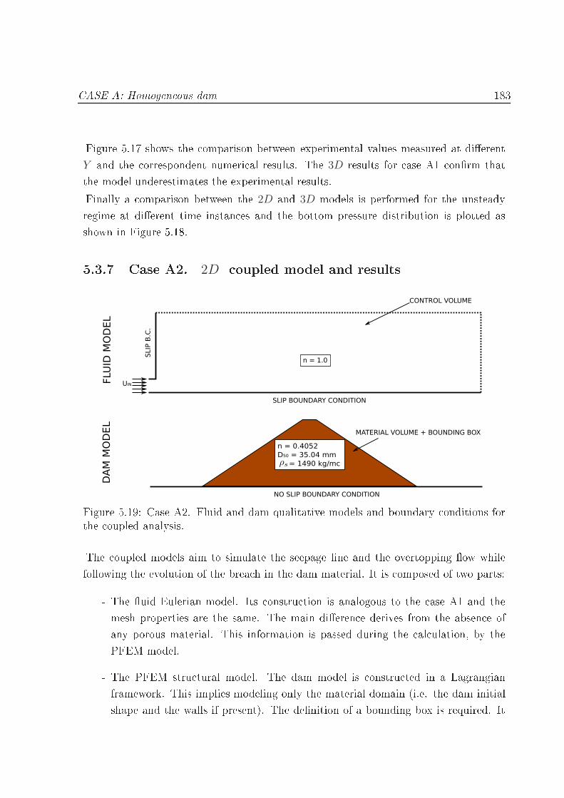
CASE A: Homogeneous dam 183Figure 5.17 shows the omparison between experimental values measured at dierentY and the orrespondent numeri al results. The 3D results for ase A1 onrm thatthe model underestimates the experimental results.Finally a omparison between the 2D and 3D models is performed for the unsteadyregime at dierent time instan es and the bottom pressure distribution is plotted asshown in Figure 5.18.5.3.7 Case A2. 2D oupled model and results

NO SLIP BOUNDARY CONDITION

n = 0.4052

D50 = 35.04 mm

= 1490 kg/mc

CONTROL VOLUME

MATERIAL VOLUME + BOUNDING BOX

FLU

ID M

OD

EL

DA

M M

OD

EL

n = 1.0

UIN

SLIP BOUNDARY CONDITION

SLIP

B.C

.

Figure 5.19: Case A2. Fluid and dam qualitative models and boundary onditions forthe oupled analysis.The oupled models aim to simulate the seepage line and the overtopping ow whilefollowing the evolution of the brea h in the dam material. It is omposed of two parts:- The uid Eulerian model. Its onstru tion is analogous to the ase A1 and themesh properties are the same. The main dieren e derives from the absen e ofany porous material. This information is passed during the al ulation, by thePFEM model.- The PFEM stru tural model. The dam model is onstru ted in a Lagrangianframework. This implies modeling only the material domain (i.e. the dam initialshape and the walls if present). The denition of a bounding box is required. It

184 Failure analysis of s ale models of ro kll dams under seepage onditionssets the maximum al ulation domain. If a node exits the bounding box is nolonger al ulated and is deleted.Remark 22. A preliminary remark on the interpretation of the experimental datashould be made here. The experimental B length of failure is by denition the horizontalproje tion of the position of the higher parti les that moves. This movement is notquantied. In the present work it was assumed that a parti le is to be onsideredmoved if its total displa ement is higher than the average dimension of the granularmaterial (3.0cm). This hoi e is arguable and, as it will be shown later on, it oftenmakes our model too deformable. Nevertheless this empiri al riterion was used in allthe models analyzed in order to allow a omparative analysis.Figure 5.20: Case A2. 2D mesh of the dam model. 3.400 linear triangular elements.In Figure 5.19 a s hemati view of the uid and stru ture boundary onditions is shown.The mesh used for the uid model is the same used in ase A1, whereas for the stru turalmodel, the mesh is omposed of 3 400 linear triangular elements (Figure 5.20).The photogrammetri analysis of the A ases was also available and helped the om-parison between experimental and numeri al results. Figures 5.21-5.23 show on the leftthe digital model derived by the photogrammetri analysis, and on the right the ontourll of the displa ements. The olored area indi ates the displa ements larger than 3cm.The reason for this hoi e is explained in Remark 22. A very good agreement is observedbetween experimental and numeri al length of failure in the three ases.Looking at the pressure head distribution (gures 5.24-5.24), the experimental bottompressure head is underestimated by the numeri al one. This aspe t is more relevant thanin ase A1. It might be the signal of an internal variation of the material onditions(su h as porosity or permeability) that is not taken into a ount in the model.Figure 5.26 shows that in ase A23, the pressure head presents a lower experimentalvalue where the water exits the dam. The ontra tion of the ux an be indu ed by

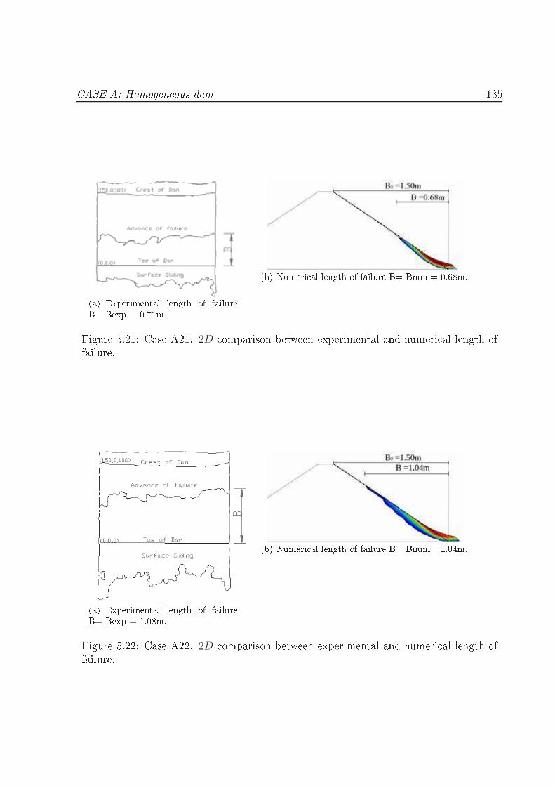
CASE A: Homogeneous dam 185

(a) Experimental length of failureB= Bexp = 0.71m. (b) Numeri al length of failure B= Bnum= 0.68m.Figure 5.21: Case A21. 2D omparison between experimental and numeri al length offailure.

(a) Experimental length of failureB= Bexp = 1.08m.(b) Numeri al length of failure B= Bnum= 1.04m.

Figure 5.22: Case A22. 2D omparison between experimental and numeri al length offailure.

186 Failure analysis of s ale models of ro kll dams under seepage onditions

(a) Experimental length of failureB= Bexp = 1.56m.(b) Numeri al length of failure B= Bnum= 1.58m.

Figure 5.23: Case A23. 2D omparison between experimental and numeri al length offailure.0.0 0.5 1.0 1.5 2.0 2.5 3.0 3.5

[m]0.0

0.2

0.4

0.6

0.8

1.0

PRES

SURE

[m]

Q=51.75l/sOriginal dam shapeNumerical resultsExp results

Figure 5.24: Case A21. Bottom pressure distribution at stationary regime for Q =51.75l/s. Porosity n = 0.4, D50 = 35mm. Numeri al and experimental omparison.Q [l/s] Bexp Bnum ErrorCase A21 51.75 0.71 0.68 4.2%Case A22 69.07 1.08 1.04 3.7%Case A23 90.68 1.56 1.58 1.3%Table 5.5: Case A2. Comparison between experimental (Bexp) and numeri al (Bnum)length of failure.

CASE A: Homogeneous dam 187

0.0 0.5 1.0 1.5 2.0 2.5 3.0 3.5[m]

0.0

0.2

0.4

0.6

0.8

1.0

PRES

SURE

[m]

Q=69.07l/sOriginal dam shapeNumerical resultsExp results

Figure 5.25: Case A22. Bottom pressure distribution at stationary regime for Q =69.07l/s. Porosity n = 0.4, D50 = 35mm. Numeri al and experimental omparison.the absen e of the ro kll that owed away during the failure pro ess. This leads tothe on lusion that the failed material in the numeri al model is more rigid than in thereal ase. Its a umulation over the original toe of the dam indu es a higher value ofpressure than in the experiment.

0.0 0.5 1.0 1.5 2.0 2.5 3.0 3.5[m]

0.0

0.2

0.4

0.6

0.8

1.0

PRES

SURE

[m]

Q=90.68l/sOriginal dam shapeNumerical resultsExp results

Figure 5.26: Case A23. Bottom pressure distribution at stationary regime for Q =90.68l/s. Porosity n = 0.4, D50 = 35mm. Numeri al and experimental omparison.5.3.8 Case A2. 2D sequen e of in remental dis hargesThe ode was on eived to analyze the onsequen e of transitory in oming dis harges,allowing inserting ooding urves as an input. Unfortunately this apability has notbeen exploited in the examples presented be ause the experimental results where givenfor the stationary regime and no omparison an be made in the transitory regime.Fortunately in the last months, the UPM partners in the E-DAMS proje t have been

188 Failure analysis of s ale models of ro kll dams under seepage onditionsperforming some experiments onsidering variable in oming dis harges a ording to ahydrogram.

0 50 100 150 200 250 300 350 400TIME [s]

0

20

40

60

80

INLE

T D

ISCH

ARG

E [l/

s]

Q=25.26l/s

Q=51.75l/s

Q=69.07l/s

Figure 5.27: Imposed in oming dis harge in fun tion of time.As a preliminary test, ases A1-A21-A22 were run in sequen e leaving the su ient timefor the intermediate stationary regime to be a hieved. The imposed urve representingthe inlet dis harge in fun tion of time, is reported in Figure 5.27. The pressure head in orresponden e of two pressure sensors lo ation is registered as an be seen in Figure5.28. The two points are lo ated at 2.2m and 2.7m from the upstream toe of the dam.The dotted line in the graph is the stationary value of pressure read from the piezometersin the ases A1, A21 and A22 respe tively. Also in this ase the numeri al resultsunderestimate the experimental ones and the error is analogous to the one presented inthe previous se tion.5.3.9 Case A2. 3D oupled model and resultsSome preliminary results have been obtained also in 3D. The uid and stru tural modelshave been developed a ording to what explained in Se tion 5.3.7 for the 2D validation.On the other hand, the deformation of the dam is not so lear as in the 2D ase. Thishappens be ause the deformation is partially skewed by the remeshing at ea h time step.As explained in Se tion 3.7, remeshing is a key point of PFEM. In fa t this method wasoriginally on eived to treat Newtonian free surfa e problems where the regeneration ofthe mesh is always required. This is not the ase of the present non-Newtonian algorithmwhere in most of the steps all the nodes are in the unyielded region and do not move.

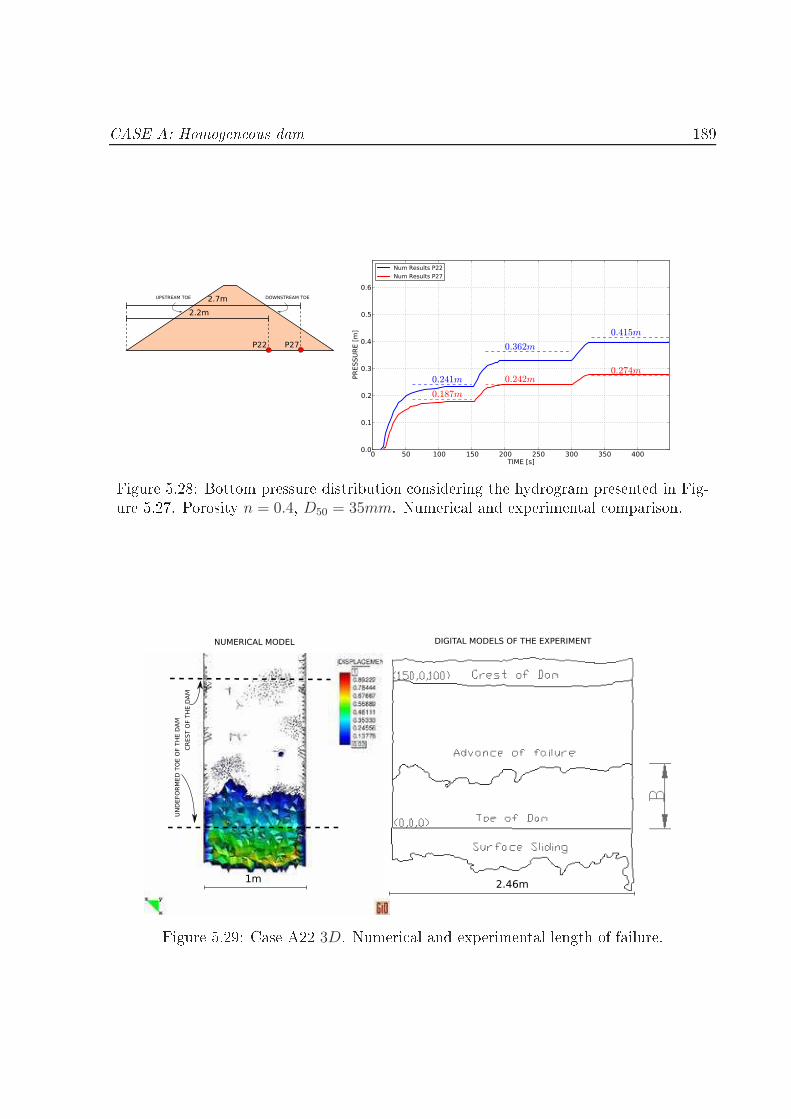
CASE A: Homogeneous dam 189DOWNSTREAM TOE

2.2m

2.7m

P22 P27

UPSTREAM TOE

0 50 100 150 200 250 300 350 400TIME [s]

0.0

0.1

0.2

0.3

0.4

0.5

0.6

PRES

SURE

[m]

0.241m

0.362m

0.415m

0.187m

0.242m0.274m

Num Results P22Num Results P27

Figure 5.28: Bottom pressure distribution onsidering the hydrogram presented in Fig-ure 5.27. Porosity n = 0.4, D50 = 35mm. Numeri al and experimental omparison.

CR

EST O

F T

HE D

AM

UN

DEFO

RM

ED

TO

E O

F T

HE D

AM

1m2.46m

NUMERICAL MODEL DIGITAL MODELS OF THE EXPERIMENT

Figure 5.29: Case A22 3D. Numeri al and experimental length of failure.

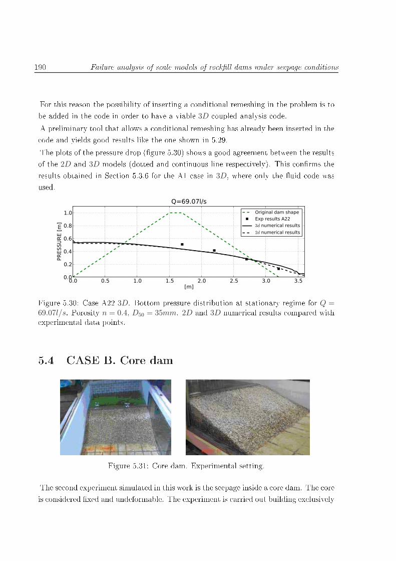
190 Failure analysis of s ale models of ro kll dams under seepage onditionsFor this reason the possibility of inserting a onditional remeshing in the problem is tobe added in the ode in order to have a viable 3D oupled analysis ode.A preliminary tool that allows a onditional remeshing has already been inserted in the ode and yields good results like the one shown in 5.29.The plots of the pressure drop (gure 5.30) shows a good agreement between the resultsof the 2D and 3D models (dotted and ontinuous line respe tively). This onrms theresults obtained in Se tion 5.3.6 for the A1 ase in 3D, where only the uid ode wasused.0.0 0.5 1.0 1.5 2.0 2.5 3.0 3.5

[m]0.0

0.2

0.4

0.6

0.8

1.0

PRES

SURE

[m]

Q=69.07l/sOriginal dam shapeExp results A223d numerical results2d numerical results

Figure 5.30: Case A22 3D. Bottom pressure distribution at stationary regime for Q =69.07l/s. Porosity n = 0.4, D50 = 35mm. 2D and 3D numeri al results ompared withexperimental data points.5.4 CASE B. Core dam

Figure 5.31: Core dam. Experimental setting.The se ond experiment simulated in this work is the seepage inside a ore dam. The oreis onsidered xed and undeformable. The experiment is arried out building ex lusively

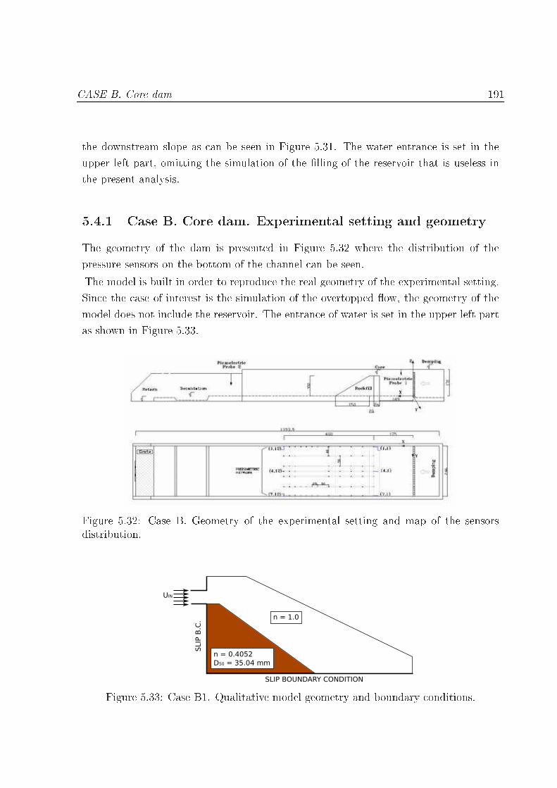
CASE B. Core dam 191the downstream slope as an be seen in Figure 5.31. The water entran e is set in theupper left part, omitting the simulation of the lling of the reservoir that is useless inthe present analysis.5.4.1 Case B. Core dam. Experimental setting and geometryThe geometry of the dam is presented in Figure 5.32 where the distribution of thepressure sensors on the bottom of the hannel an be seen.The model is built in order to reprodu e the real geometry of the experimental setting.Sin e the ase of interest is the simulation of the overtopped ow, the geometry of themodel does not in lude the reservoir. The entran e of water is set in the upper left partas shown in Figure 5.33.

Figure 5.32: Case B. Geometry of the experimental setting and map of the sensorsdistribution.

SLIP BOUNDARY CONDITION

SLIP

B.C

.

UIN

n = 0.4052

D50 = 35.04 mm

n = 1.0

Figure 5.33: Case B1. Qualitative model geometry and boundary onditions.

192 Failure analysis of s ale models of ro kll dams under seepage onditionsA slip boundary ondition is imposed on the bottom of the hannel and on the oreside.5.4.2 Case B1a. Core dam. 2D numeri al model and results

Figure 5.34: Case B1a. Mesh used in the al ulation.The mesh used for the al ulation an be seen in Figure 5.34. It has 14 859 lineartriangular elements. The omparison between experimental and numeri al pressureheads an be observed in Figure 5.35.A renement of the mesh is performed in the riti al zones of the falling of the waterand near the bottom of the hannel. The reason for that hoi e will be explained inSe tion 5.5.2 when des ribing ase C1.

0.0 0.5 1.0 1.5 2.0[m]

0.0

0.2

0.4

0.6

0.8

1.0

PRES

SURE

[m]

Q=5.93l/sDam shapeNumerical resultsExperimental results

Figure 5.35: Case B1a. Bottom pressure distribution at stationary regime for Q =5.93l/s. Porosity n = 0.4, D50 = 35mm. Numeri al and experimental omparison.

CASE B. Core dam 193Case B presents an additional di ulty in the uid dynami problem. It is parti ularly hallenging to simulate orre tly the falling jet of water (espe ially if the in oming watervelo ity is very slow), without suering serious mass loss. The good agreement betweenexperimental and numeri al pressure heads onrms that this problem an be a uratelymodeled with the method developed in this work. This is onrmed in the 3D simulationof ase B1a in Se tion 5.4.4.5.4.3 Cases B1b and B1 . Core dam. Comparison with theo-reti al Ergun modelIt has been observed that the numeri al pressure head gives lower values than the exper-imental ones. To verify if the problem an be attributed to the hoi e of the resistan elaw, a omparison with the theoreti al results is performed a ording to the work ofLopez Verdejo [125. In order to do that a slightly dierent geometry is taken intoa ount. The dam studied is made of the same material as the one presented in theprevious se tions but the height of the dam is 0.5m and the length of the downstreamslope is 1.5m. The slope ratio is H3 : V 1.The mesh used is shown in Figure 5.36. It has 2 865 nodes and 5 728 linear triangularelements.

Figure 5.36: Case B1(b- ).Mesh used in the al ulation.The theoreti al solution for an in oming dis harge of 4.0l/s and 16.7l/s is plotted in reddotted line in Figures 5.37 and 5.38 respe tively. The numeri al approximation is very lose to the Ergun theoreti al one as expe ted. Both these urves underestimate theexperimental values. This onrms that Ergun model might not be the best hoi e forthe resistan e law of this kind of problem. In order to over ome this issue the next stepwill be to modify the ode in order to let the user insert a ustom quadrati resistan e

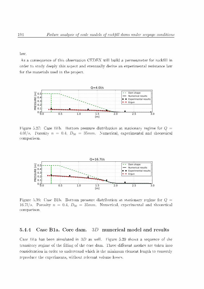
194 Failure analysis of s ale models of ro kll dams under seepage onditionslaw.As a onsequen e of this observation CEDEX will build a permeameter for ro kll inorder to study deeply this aspe t and eventually derive an experimental resistan e lawfor the materials used in the proje t.0.0 0.5 1.0 1.5 2.0 2.5 3.0

[m]0.00.10.20.30.40.5

PRES

SURE

[m]

Q=4.0l/sDam shapeNumerical resultsExperimental resultsErgun

Figure 5.37: Case B1b. Bottom pressure distribution at stationary regime for Q =4.0l/s. Porosity n = 0.4, D50 = 35mm. Numeri al, experimental and theoreti al omparison.

0.0 0.5 1.0 1.5 2.0 2.5 3.0[m]

0.00.10.20.30.40.5

PRES

SURE

[m]

Q=16.7l/sDam shapeNumerical resultsExperimental resultsErgun

Figure 5.38: Case B1b. Bottom pressure distribution at stationary regime for Q =16.7l/s. Porosity n = 0.4, D50 = 35mm. Numeri al, experimental and theoreti al omparison.5.4.4 Case B1a. Core dam. 3D numeri al model and resultsCase B1a has been simulated in 3D as well. Figure 5.39 shows a sequen e of thetransitory regime of the lling of the ore dam. Three dierent meshes are taken into onsideration in order to understand whi h is the minimum element length to orre tlyreprodu e the experiments, without relevant volume losses.

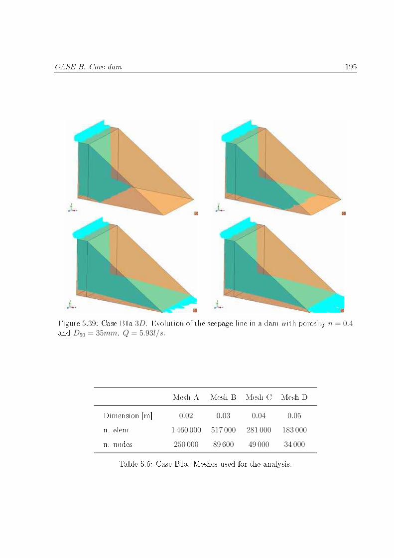
CASE B. Core dam 195

Figure 5.39: Case B1a 3D. Evolution of the seepage line in a dam with porosity n = 0.4and D50 = 35mm. Q = 5.93l/s.Mesh A Mesh B Mesh C Mesh DDimension [m 0.02 0.03 0.04 0.05n. elem 1 460 000 517 000 281 000 183 000n. nodes 250 000 89 600 49 000 34 000Table 5.6: Case B1a. Meshes used for the analysis.

196 Failure analysis of s ale models of ro kll dams under seepage onditionsThe hara teristi s of the four meshes analyzed are summarized in Table 5.6. Therenement is performed only in the dam volume, whereas the dimension of the elementsis kept xed in the rest of the domain as it an be observed in Figure 5.40.(a) Mesh A (b) Mesh B( ) Mesh C (d) Mesh DFigure 5.40: Case A1. Meshes used in the analysis of mesh sensitivity. The hara ter-isti s of the meshes an be found in Table 5.6.Figure 5.41 shows the pressure heads for the dierent mesh sizes. The onvergen e isa hieved when the mesh is ner than 0.03m. For larger meshes the volume onservationis seriously ompromised. This loss takes pla e when the ux falls down verti ally.Therefore parti ular are should be taken in the renement for the analysis of a oredam.5.4.5 Case B2. Core dam. Coupled model and resultsThe onstru tion of the models for the oupled ase is analogous to what already ex-plained in Se tion 5.3.7 for the A2 ase. A s hemati representation of the boundary onditions an be found in Figure 5.42.Figure 5.43 shows the Lagrangian mesh used in the al ulation. It has 8 000 lineartriangular elements.

CASE B. Core dam 197

0.0 0.5 1.0 1.5 2.0[m]

0.0

0.2

0.4

0.6

0.8

1.0

PRES

SURE

[m]

Q=5.93l/sDam shapeExperimental resultsMesh A (0.02m)Mesh B (0.03m)Mesh C (0.04m)Mesh D (0.05m)

Figure 5.41: Case B1a (3D). Bottom pressure distribution at stationary regime forQ = 5.93l/s. Porosity n = 0.4, D50 = 35mm. Numeri al, experimental and theoreti al omparison.

NO SLIP BOUNDARY CONDITION

n = 0.4052

D50 = 35.04 mm

= 1490 kg/mc

CONTROL VOLUME

MATERIAL VOLUME + BOUNDING BOX

FLU

ID M

OD

EL

DA

M M

OD

EL

SLIP BOUNDARY CONDITION

SLIP

B.C

.

UIN

n = 1.0

Figure 5.42: Case B2. Fluid and dam qualitative models and boundary onditions forthe oupled analysis.

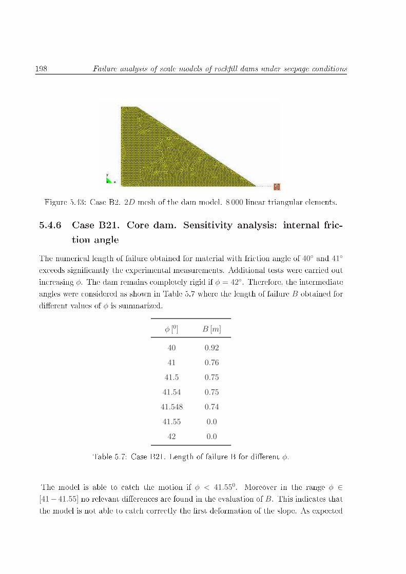
198 Failure analysis of s ale models of ro kll dams under seepage onditions

Figure 5.43: Case B2. 2D mesh of the dam model. 8 000 linear triangular elements.5.4.6 Case B21. Core dam. Sensitivity analysis: internal fri -tion angleThe numeri al length of failure obtained for material with fri tion angle of 40 and 41ex eeds signi antly the experimental measurements. Additional tests were arried outin reasing φ. The dam remains ompletely rigid if φ = 42. Therefore, the intermediateangles were onsidered as shown in Table 5.7 where the length of failure B obtained fordierent values of φ is summarized.φ [0] B [m]

40 0.92

41 0.76

41.5 0.75

41.54 0.75

41.548 0.74

41.55 0.0

42 0.0Table 5.7: Case B21. Length of failure B for dierent φ.The model is able to at h the motion if φ < 41.550. Moreover in the range φ ∈[41− 41.55] no relevant dieren es are found in the evaluation of B. This indi ates thatthe model is not able to at h orre tly the rst deformation of the slope. As expe ted

CASE B. Core dam 199no relevant hanges are observed in the pressure head of the onsidered ases (gure5.44).

0.0 0.5 1.0 1.5 2.0 2.5[m]

0.0

0.2

0.4

0.6

0.8

1.0

PRES

SURE

[m]

Q=19.36l/sDam shapeExperimental resultsNumerical results =400

Numerical results =410

Numerical results =41.50

Numerical results =41.540

Numerical results =41.5480

Numerical results =41.550

Numerical results =420

Figure 5.44: Case B21. Bottom pressure distribution at stationary regime for Q =19.36l/s. Porosity n = 0.4, D50 = 35mm. Numeri al and experimental omparison fordierent internal fri tion angles φ.The a ura y improves for ases B22 and B23 as explained in the next se tions. Thisfa t oin ides with what was observed experimentally: the length of failure indu ed bythe lower step of dis harge presents a high data s atter whereas the failure a hieves the rest always at the same dis harge level.5.4.7 Case B2 with φ = 41Sin e the dieren e in the length of failure is not so relevant if φ ∈ [41 − 41.55], theinternal fri tion angle adopted for ase B2 is φ = 41.Figures 5.45-5.47 show the omparison between experimental and numeri al dam de-formation at ea h step of dis harge for φ = 41. The error in the evaluation of B isprogressively redu ed when in reasing the dis harge as detailed in Table 5.8.An additional onsideration an be made looking at the pressure head distribution ofthe three ases shown in Figures 5.48-5.50. As for the A2 ase, the amount of movedro kll is lower in the simulation than in the experiments. In fa t the higher value ofnumeri al pressure at the toe of the dam indi ates that granular material is presentover the sensor position (i.e. the resistan e given by the grains in reases the water leveland the pressure head as well). This seems to indi ate that the material settles fasterthan in the experiment. It may be the onsequen e of the vis o-rigid onstitutive modeladopted.

200 Failure analysis of s ale models of ro kll dams under seepage onditions

(a) Experimental length of failureBexp = 0.32m. (b) Numeri al length of failure B= Bnum= 0.76m.Figure 5.45: Case B21. 2D omparison between experimental and numeri al length offailure.

(a) Experimental length of failureBexp = 0.68m. (b) Numeri al length of failure B= Bnum= 0.90m.Figure 5.46: Case B22. 2D omparison between experimental and numeri al length offailure.

(a) Experimental length of failureBexp = 1.00m. (b) Numeri al length of failure B= Bnum= 1.02m.Figure 5.47: Case B23. 2D omparison between experimental and numeri al length offailure.

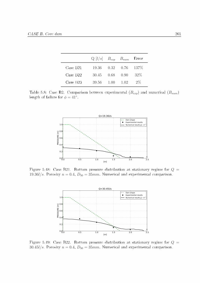
CASE B. Core dam 201Q [l/s] Bexp Bnum ErrorCase B21 19.36 0.32 0.76 137%Case B22 30.45 0.68 0.90 32%Case B23 39.56 1.00 1.02 2%Table 5.8: Case B2. Comparison between experimental (Bexp) and numeri al (Bnum)length of failure for φ = 41.

0.0 0.5 1.0 1.5 2.0 2.5[m]

0.0

0.2

0.4

0.6

0.8

1.0

PRES

SURE

[m]

Q=19.36l/sDam shapeExperimental resultsNumerical results =410

Figure 5.48: Case B21. Bottom pressure distribution at stationary regime for Q =19.36l/s. Porosity n = 0.4, D50 = 35mm. Numeri al and experimental omparison.

0.0 0.5 1.0 1.5 2.0 2.5[m]

0.0

0.2

0.4

0.6

0.8

1.0

PRES

SURE

[m]

Q=30.45l/sDam shapeExperimental resultsNumerical results =410

Figure 5.49: Case B22. Bottom pressure distribution at stationary regime for Q =30.45l/s. Porosity n = 0.4, D50 = 35mm. Numeri al and experimental omparison.

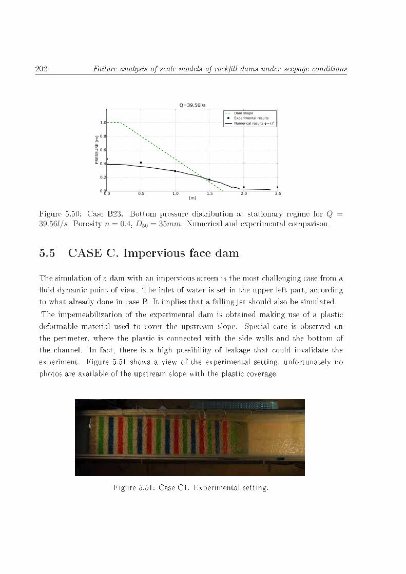
202 Failure analysis of s ale models of ro kll dams under seepage onditions

0.0 0.5 1.0 1.5 2.0 2.5[m]

0.0

0.2

0.4

0.6

0.8

1.0

PRES

SURE

[m]

Q=39.56l/sDam shapeExperimental resultsNumerical results =410

Figure 5.50: Case B23. Bottom pressure distribution at stationary regime for Q =39.56l/s. Porosity n = 0.4, D50 = 35mm. Numeri al and experimental omparison.5.5 CASE C. Impervious fa e damThe simulation of a dam with an impervious s reen is the most hallenging ase from auid dynami point of view. The inlet of water is set in the upper left part, a ordingto what already done in ase B. It implies that a falling jet should also be simulated.The impemeabilization of the experimental dam is obtained making use of a plasti deformable material used to over the upstream slope. Spe ial are is observed onthe perimeter, where the plasti is onne ted with the side walls and the bottom ofthe hannel. In fa t, there is a high possibility of leakage that ould invalidate theexperiment. Figure 5.51 shows a view of the experimental setting, unfortunately nophotos are available of the upstream slope with the plasti overage.

Figure 5.51: Case C1. Experimental setting.

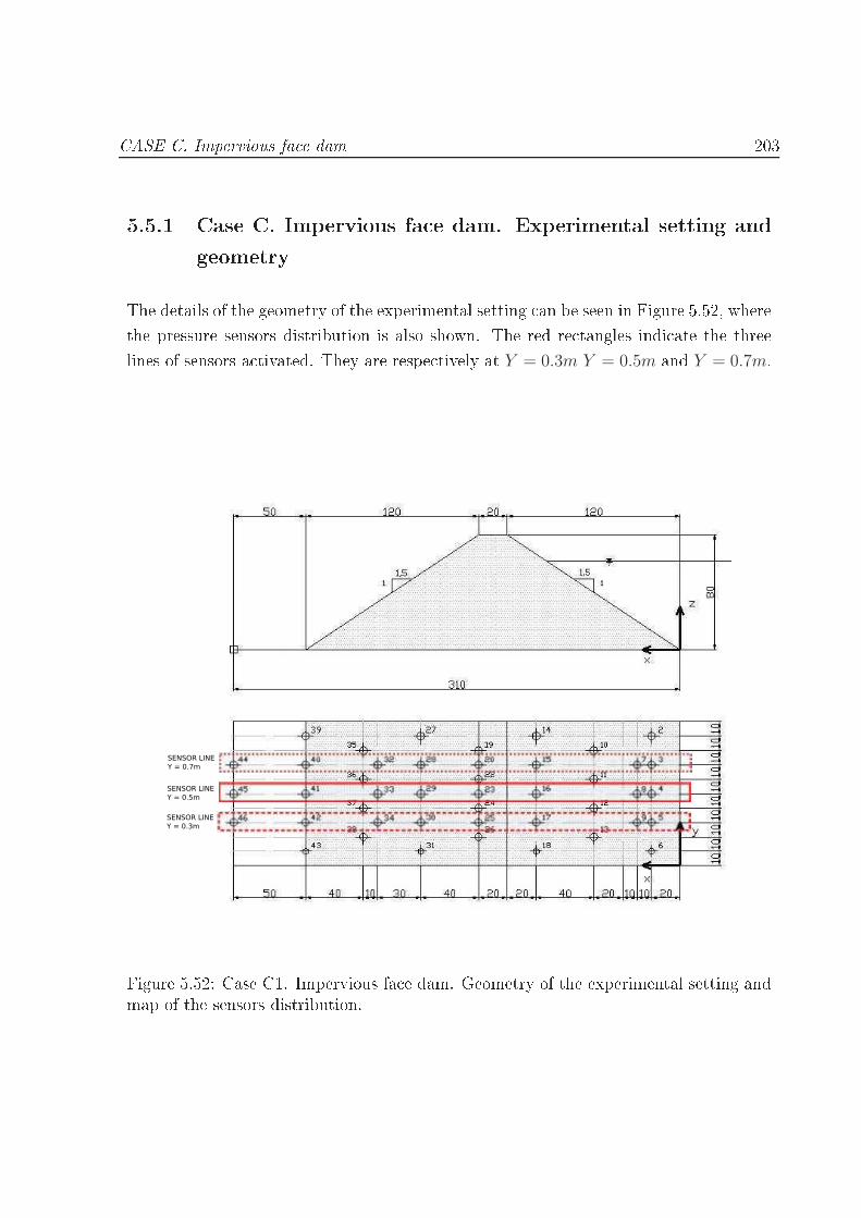
CASE C. Impervious fa e dam 2035.5.1 Case C. Impervious fa e dam. Experimental setting andgeometryThe details of the geometry of the experimental setting an be seen in Figure 5.52, wherethe pressure sensors distribution is also shown. The red re tangles indi ate the threelines of sensors a tivated. They are respe tively at Y = 0.3m Y = 0.5m and Y = 0.7m.

SENSOR LINE

Y = 0.7m

SENSOR LINE

Y = 0.5m

SENSOR LINE

Y = 0.3m

Figure 5.52: Case C1. Impervious fa e dam. Geometry of the experimental setting andmap of the sensors distribution.

204 Failure analysis of s ale models of ro kll dams under seepage onditions5.5.2 Case C1. Impervious fa e dam. Un oupled model andresultsIn order to optimize the omputational domain, the upstream reservoir is not simulatedand the entran e of water is dire tly set in the upper left part, at the rest level, as shownin Figure 5.53. The upstream s reen is therefore onsidered perfe tly impermeable andit is simulated as a rigid wall with a slip ondition.n = 1.0

UIN

SLIP BOUNDARY CONDITION

SCREEN

n = 0.4052

D50 = 35.04 mmSLI

P B.C

.

Figure 5.53: Impervious fa e dam. Qualitative model geometry and boundary ondi-tions.The rest of the boundary onditions are similar to those of the previous models andthey are s hemati ally presented in Figure 5.53. A qualitative geometry is also shownin the image.It has been experimentally observed that no deformation of the downstream slope o ursup to a dis harge of 5.71l/s. Mesh A Mesh B Mesh C Mesh DDimension [m 0.03 0.02 0.015 0.01n. elem 4 700 8 500 13 000 20 000n. nodes 2 900 4 200 6 800 10 000Table 5.9: Case C1. Meshes used in the analysis.Dierent mesh are used in order to identify the minimum element size that yields a orre t onservation of the uid volume. Their hara teristi s are summarized in Table5.9 and they are shown in Figure 5.54. The rst mesh taken into onsideration is meshA shown in Figure 5.54 where the average dimension of the elements is set to 0.03m.

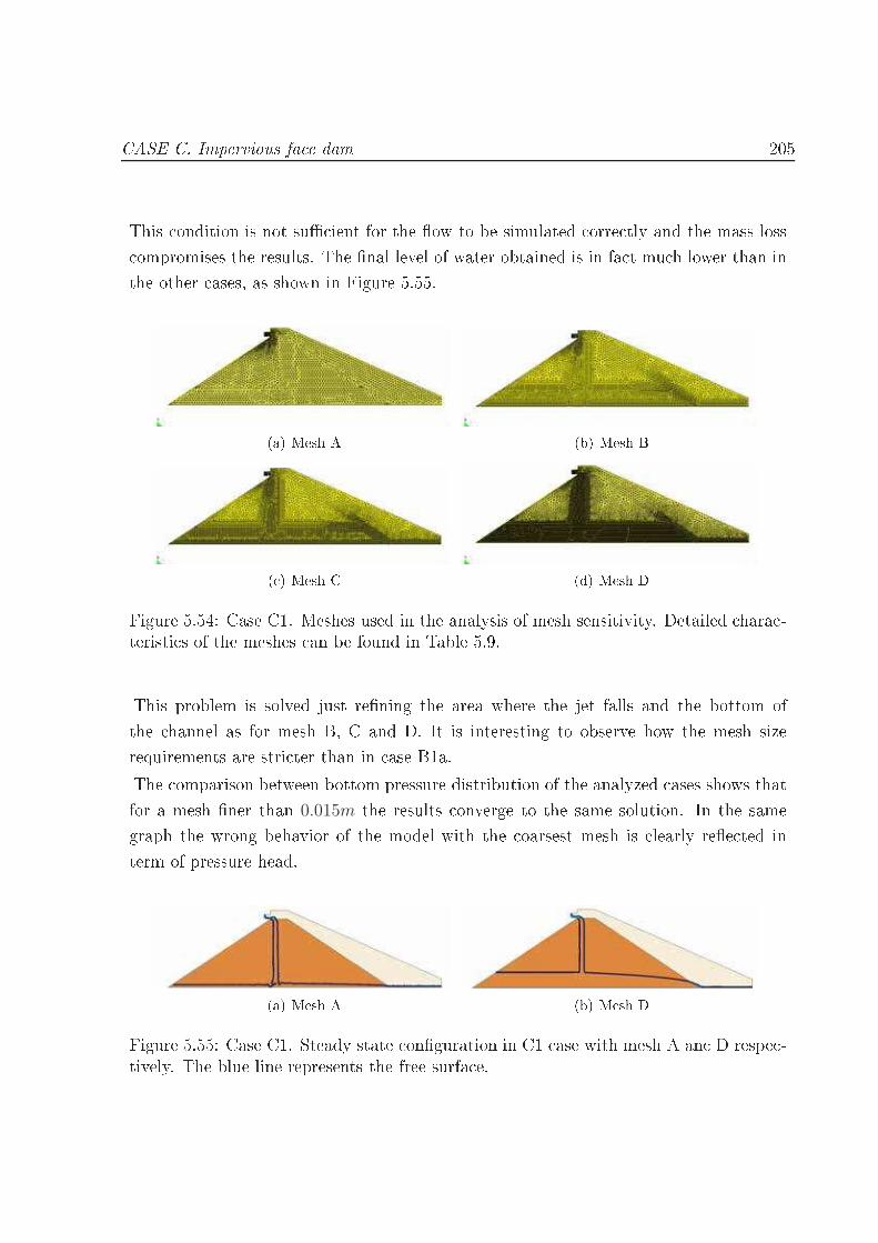
CASE C. Impervious fa e dam 205This ondition is not su ient for the ow to be simulated orre tly and the mass loss ompromises the results. The nal level of water obtained is in fa t mu h lower than inthe other ases, as shown in Figure 5.55.(a) Mesh A (b) Mesh B( ) Mesh C (d) Mesh DFigure 5.54: Case C1. Meshes used in the analysis of mesh sensitivity. Detailed hara -teristi s of the meshes an be found in Table 5.9.This problem is solved just rening the area where the jet falls and the bottom ofthe hannel as for mesh B, C and D. It is interesting to observe how the mesh sizerequirements are stri ter than in ase B1a.The omparison between bottom pressure distribution of the analyzed ases shows thatfor a mesh ner than 0.015m the results onverge to the same solution. In the samegraph the wrong behavior of the model with the oarsest mesh is learly ree ted interm of pressure head.(a) Mesh A (b) Mesh DFigure 5.55: Case C1. Steady state onguration in C1 ase with mesh A an D respe -tively. The blue line represents the free surfa e.

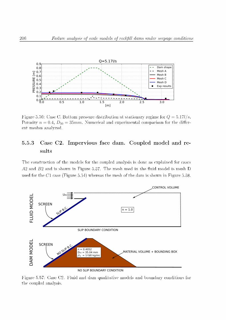
206 Failure analysis of s ale models of ro kll dams under seepage onditions

0.0 0.5 1.0 1.5 2.0 2.5 3.0[m]

0.00.10.20.30.40.50.60.70.80.9

PRES

SURE

[m]

Q=5.17l/sDam shapeMesh AMesh BMesh CMesh DExp results

Figure 5.56: Case C. Bottom pressure distribution at stationary regime for Q = 5.17l/s.Porosity n = 0.4, D50 = 35mm. Numeri al and experimental omparison for the dier-ent meshes analyzed.5.5.3 Case C2. Impervious fa e dam. Coupled model and re-sultsThe onstru tion of the models for the oupled analysis is done as explained for asesA2 and B2 and is shown in Figure 5.57. The mesh used in the uid model is mesh Dused for the C1 ase (Figure 5.54) whereas the mesh of the dam is shown in Figure 5.58.

n = 0.4052

D50 = 35.04 mm

= 10 kg/mc

NO SLIP BOUNDARY CONDITION

SCREEN

NO SLIP

B.C

.

n = 1.0

UIN

SLIP BOUNDARY CONDITION

SCREEN

SLIP B

.C.

CONTROL VOLUME

MATERIAL VOLUME + BOUNDING BOX

FLU

ID M

OD

EL

DA

M M

OD

EL

Figure 5.57: Case C2. Fluid and dam qualitative models and boundary onditions forthe oupled analysis.

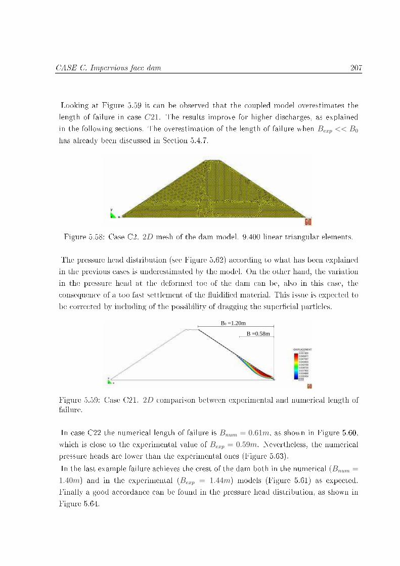
CASE C. Impervious fa e dam 207Looking at Figure 5.59 it an be observed that the oupled model overestimates thelength of failure in ase C21. The results improve for higher dis harges, as explainedin the following se tions. The overestimation of the length of failure when Bexp << B0has already been dis ussed in Se tion 5.4.7.Figure 5.58: Case C2. 2D mesh of the dam model. 9.400 linear triangular elements.The pressure head distribution (see Figure 5.62) a ording to what has been explainedin the previous ases is underestimated by the model. On the other hand, the variationin the pressure head at the deformed toe of the dam an be, also in this ase, the onsequen e of a too fast settlement of the uidied material. This issue is expe ted tobe orre ted by in luding of the possibility of dragging the super ial parti les.

B0 =1.20m

B =0.58m

Figure 5.59: Case C21. 2D omparison between experimental and numeri al length offailure.In ase C22 the numeri al length of failure is Bnum = 0.61m, as shown in Figure 5.60,whi h is lose to the experimental value of Bexp = 0.59m. Nevertheless, the numeri alpressure heads are lower than the experimental ones (Figure 5.63).In the last example failure a hieves the rest of the dam both in the numeri al (Bnum =

1.40m) and in the experimental (Bexp = 1.44m) models (Figure 5.61) as expe ted.Finally a good a ordan e an be found in the pressure head distribution, as shown inFigure 5.64.

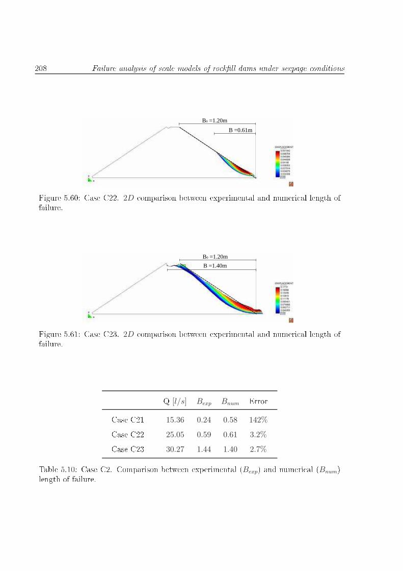
208 Failure analysis of s ale models of ro kll dams under seepage onditionsB0 =1.20m

B =0.61m

Figure 5.60: Case C22. 2D omparison between experimental and numeri al length offailure.B0 =1.20m

B =1.40m

Figure 5.61: Case C23. 2D omparison between experimental and numeri al length offailure.Q [l/s] Bexp Bnum ErrorCase C21 15.36 0.24 0.58 142%Case C22 25.05 0.59 0.61 3.2%Case C23 30.27 1.44 1.40 2.7%Table 5.10: Case C2. Comparison between experimental (Bexp) and numeri al (Bnum)length of failure.

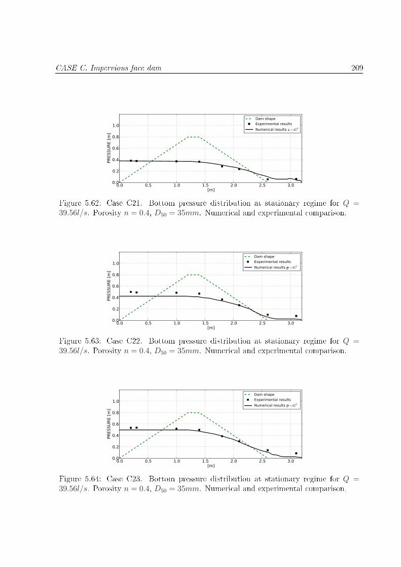
CASE C. Impervious fa e dam 209

0.0 0.5 1.0 1.5 2.0 2.5 3.0[m]

0.0

0.2

0.4

0.6

0.8

1.0

PRES

SURE

[m]

Q=15.36l/sDam shapeExperimental resultsNumerical results =410

Figure 5.62: Case C21. Bottom pressure distribution at stationary regime for Q =39.56l/s. Porosity n = 0.4, D50 = 35mm. Numeri al and experimental omparison.

0.0 0.5 1.0 1.5 2.0 2.5 3.0[m]

0.0

0.2

0.4

0.6

0.8

1.0

PRES

SURE

[m]

Q=25.05l/sDam shapeExperimental resultsNumerical results =410

Figure 5.63: Case C22. Bottom pressure distribution at stationary regime for Q =39.56l/s. Porosity n = 0.4, D50 = 35mm. Numeri al and experimental omparison.

0.0 0.5 1.0 1.5 2.0 2.5 3.0[m]

0.0

0.2

0.4

0.6

0.8

1.0

PRES

SURE

[m]

Q=30.27l/sDam shapeExperimental resultsNumerical results =410

Figure 5.64: Case C23. Bottom pressure distribution at stationary regime for Q =39.56l/s. Porosity n = 0.4, D50 = 35mm. Numeri al and experimental omparison.

210 Failure analysis of s ale models of ro kll dams under seepage onditions5.6 Con lusions and future workIn this work a novel approa h for the simulation of the onset of failure of downstreamslopes in ro kll dams is presented. The dynami evolution of seepage and the freesurfa e ow both upstream and downstream the dam are simultaneously analyzed. Thisis done using the edge-based ode presented in Chapter 2. The stru tural response isevaluated with a vis o-rigid onstitutive model. As a failure riterion, Mohr Coulombhas been adopted. The ro kll is treated as a highly vis ous non-Newtonian uid (thereason for this hoi e is explained in Chapter 4). The vis osity drasti ally de reaseswhen, due to the hydrodynami for es, the yield stress is ex eeded. When this happensfailure o urs and the material starts to ow. The uid-stru ture oupling is performedusing a fully staggered s heme and a proje tion tool between non-mat hing meshes. Inwhat follows the on lusions and the future work on erning the validation presented inthis hapter are detailed• The uid module.

1. There is a good agreement between experimental and numeri al pressureheads for the undeformed ases (A1, B1, C1) both in 2D and 3D. Never-theless the numeri al results always slightly underestimate the experimentalvalues. Additional numeri al experiments arried out in the framework ofXPRES and EDAMS proje ts an onrm that the pressure line is alwayslower than the experimental one, espe ially when in reasing the porosity val-ues. This aspe t, together with the omparison with theoreti al Ergun urvesshown in Se tion 5.4.3, lead to the on lusion that the Ergun oe ients un-derestimate the pressure drop in the seepage problem. In the near future, weplan to generalize the quadrati law of the Dar y non linear term ( αu+βu2)and let to the user the hoi e of the suitable α and β oe ients.2. The overestimation of the pressure head at the toe of the deformed dam( ases A2, B2, C2), might be the onsequen e of a smaller deformation ofthe failed material. Whereas the length of failure is orre tly reprodu ed, thefailed material settles faster than in the real ase and a umulates lose to theoriginal toe. In the experiments the path run by the failed ro kll materialis mu h larger (see the on lusion about the oupled model for additional omments on this issue).

Con lusions and future work 2113. The ode has a good performan e also in the hallenging ases of a fallingjet of water. The only requirement is a renement of the mesh in the fallingpart of the domain.4. Another hallenging aspe t of ases A1, B1, C1 is that the dis harges arevery low. This might represent a problem at the beginning of the simulationwhen a very thin layer of water starts lling the dam. This issue an be easily orre ted by rening the mesh lose to the bottom.5. It might be interesting to test the model with dierent materials and eventu-ally with several dierent porosities in the same dam. In this ontext somepreliminary results (not shown in the work) have been obtained using theuid ode. This aspe t is interesting be ause it will allow a more realisti representation of the ro kll slope. The onstru tion pro ess in fa t is usuallydone layer by layer and a me hani al ompa tion is performed with a rollerbefore passing to the next level. This ompa tion auses a rumbling of thesuper ial material. A thin layer is obtained on the surfa e. It is formedby parti les with average diameter mu h smaller than the rest of the ro kllleading to a dierent porosity.6. The s ale ee t is another aspe t that must be taken into a ount in thefuture. CEDEX is now building a hannel that will allow setting up dams ofup to 2 meters high (the maximum height of prototype dams built up to nowwas 1m).

• The oupled module.1. The ode represents the in remental failure of the dam when in reasing theoverspilling dis harge. It is also able to represent orre tly the ases for whi hfailure a hieves the rest of the dam. On the ontrary for lower dis harges

B is overestimated. This aspe t is also ree ted at experimental level. Infa t when repeating the same experiment, the beginning of formation of thebrea hing suers of a ertain data s atter. Conversely, the dis harge for whi hthe failure rea hes the rest is always the same.2. As already observed in the on lusions regarding the uid module, the failedmaterial settles faster than in the real ase. This an be a onsequen e of thevis o-rigid onstitutive model hosen. In fa t when the shear stress de reasesunder the yield stress threshold, the vis osity dramati ally in reases ausing

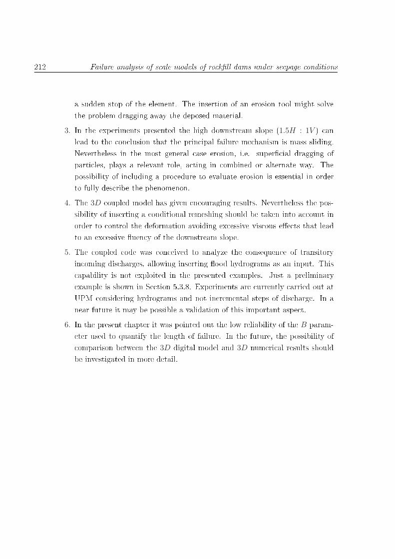
212 Failure analysis of s ale models of ro kll dams under seepage onditionsa sudden stop of the element. The insertion of an erosion tool might solvethe problem dragging away the deposed material.3. In the experiments presented the high downstream slope (1.5H : 1V ) anlead to the on lusion that the prin ipal failure me hanism is mass sliding.Nevertheless in the most general ase erosion, i.e. super ial dragging ofparti les, plays a relevant role, a ting in ombined or alternate way. Thepossibility of in luding a pro edure to evaluate erosion is essential in orderto fully des ribe the phenomenon.4. The 3D oupled model has given en ouraging results. Nevertheless the pos-sibility of inserting a onditional remeshing should be taken into a ount inorder to ontrol the deformation avoiding ex essive vis ous ee ts that leadto an ex essive uen y of the downstream slope.5. The oupled ode was on eived to analyze the onsequen e of transitoryin oming dis harges, allowing inserting ood hydrograms as an input. This apability is not exploited in the presented examples. Just a preliminaryexample is shown in Se tion 5.3.8. Experiments are urrently arried out atUPM onsidering hydrograms and not in remental steps of dis harge. In anear future it may be possible a validation of this important aspe t.6. In the present hapter it was pointed out the low reliability of the B param-eter used to quantify the length of failure. In the future, the possibility of omparison between the 3D digital model and 3D numeri al results shouldbe investigated in more detail.

Chapter 6Con lusionsIn this hapter the on lusions of the work are presented and an overview of the futurelines of resear h is made.6.1 Summary and a hievementsThe aim of this work was to development a numeri al tool for the simulation of theovertopping in ro kll dams. For that purpose three are the main points developed inthe present work (ree ted in Chapters 2, 3 and 4 respe tively):1. The development of a uid ode able to simulate the free surfa e ow over andthroughout the ro kll. The lassi al Navier-Stokes equations have been modiedto automati ally a ount for a hange in porosity values. The non linear seepageis evaluated using a quadrati form of the resistan e law. Ergun's oe ientshave been hosen. The possibility of in luding variable in oming dis harges isan essential requirement for the obje tives of the work. A xed mesh approa hhas been used and a level set te hnique has been implemented for tra king theevolution of the free surfa e both outside and inside the ro kll. Of the twoapproa hes presented in Chapter 2, the edge-based one has been hosen for itsbetter performan es in terms of omputer time.2. The implementation of a ode to simulate the behaviour of a granular non- ohesivematerial. A non- Newtonian modied Bingham law is proposed. This approa hgives the possibility of onsidering a pressure sensitive resistan e riteria. This is

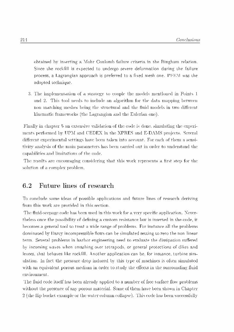
214 Con lusionsobtained by inserting a Mohr Coulomb failure riteria in the Bingham relation.Sin e the ro kll is expe ted to undergo severe deformation during the failurepro ess, a Lagrangian approa h is preferred to a xed mesh one. PFEM was theadopted te hnique.3. The implementation of a strategy to ouple the models mentioned in Points 1and 2. This tool needs to in lude an algorithm for the data mapping betweennon mat hing meshes being the stru tural and the uid models in two dierentkinemati frameworks (the Lagrangian and the Eulerian one).Finally in hapter 5 an extensive validation of the ode is done, simulating the experi-ments performed by UPM and CEDEX in the XPRES and E-DAMS proje ts. Severaldierent experimental settings have been taken into a ount. For ea h of them a sensi-tivity analysis of the main parameters has been arried out in order to understand the apabilities and limitations of the ode.The results are en ouraging onsidering that this work represents a rst step for thesolution of a omplex problem.6.2 Future lines of resear hTo on lude some ideas of possible appli ations and future lines of resear h derivingfrom this work are provided in this se tion.The uid-seepage ode has been used in this work for a very spe i appli ation. Never-theless on e the possibility of dening a ustom resistan e law is inserted in the ode, itbe omes a general tool to treat a wide range of problems. For instan e all the problemsdominated by Dar y in ompressible ows an be simulated setting to zero the non-linearterm. Several problems in harbor engineering need to evaluate the dissipation sueredby in oming waves when smashing over tetrapods, or general prote tions of dikes andlevees, that behaves like ro kll. Another appli ation an be, for instan e, turbine sim-ulation. In fa t the pressure drop indu ed by this type of ma hines is often simulatedwith an equivalent porous medium in order to study the ee ts in the surrounding uidenvironment.The uid ode itself has been already applied to a number of free surfa e ow problemswithout the presen e of any porous material. Some of them have been shown in Chapter2 (the ip bu ket example or the water olumn ollapse). This ode has been su essfully

Future lines of resear h 215used for the al ulation of the dis harge on a spillway as detailed in [112, or for thesimulation of mould lling pro esses as shown in [108.The modied Bingham model oupled with the uid ode an also be used for thesimulation of the ee t of a landslide into a reservoir. In fa t the ode naturally simulatesthe intera tion between the solid falling into the water and the resulting wave.Con erning the problem of overtopping in ro kll dams, it should be remarked thatthe whole work was on eived to easily hange the stru tural model maintaining the oupling strategy and the uid-seepage module. As a omplement of the FEM-PFEM ontinuous approa h presented in this work, the possibility of a FEM-DEM model is urrently being explored by other resear hers of the same working team.

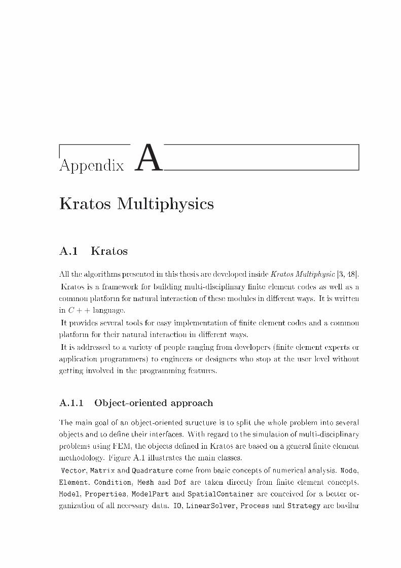
Appendix AKratos Multiphysi sA.1 KratosAll the algorithms presented in this thesis are developed insideKratos Multiphysi [3, 48.Kratos is a framework for building multi-dis iplinary nite element odes as well as a ommon platform for natural intera tion of these modules in dierent ways. It is writtenin C ++ language.It provides several tools for easy implementation of nite element odes and a ommonplatform for their natural intera tion in dierent ways.It is addressed to a variety of people ranging from developers (nite element experts orappli ation programmers) to engineers or designers who stop at the user level withoutgetting involved in the programming features.A.1.1 Obje t-oriented approa hThe main goal of an obje t-oriented stru ture is to split the whole problem into severalobje ts and to dene their interfa es. With regard to the simulation of multi-dis iplinaryproblems using FEM, the obje ts dened in Kratos are based on a general nite elementmethodology. Figure A.1 illustrates the main lasses.Ve tor, Matrix and Quadrature ome from basi on epts of numeri al analysis. Node,Element, Condition, Mesh and Dof are taken dire tly from nite element on epts.Model, Properties, ModelPart and SpatialContainer are on eived for a better or-ganization of all ne essary data. IO, LinearSolver, Pro ess and Strategy are basilar

218 Kratos Multiphysi s

Figure A.1: List of the prin ipal obje t in Kratos. Image taken from [47.dierent tools of nite element programs. Finally, Kernel and Appli ation handle thelibrary management and dene Kratos interfa e.A.1.2 Multi- layer designKratos uses a multi-layer approa h in its design. This imply that ea h obje t only inter-fa es with obje ts in the same layer or in lower ones. Layering redu es the dependen yinside the program. It helps in the maintenan e of the ode and also helps developersto understand the ode and laries their tasks.The layers stru ture has been designed to be addressed to dierent ategory of users. Itwas on eived to lead the user to work with the minimum number of layers as possible.This was done in order to redu e oni ts between users and espe ially to redu e asmu h as possible the part of the ode tou hed by ea h developer.Following the design mentioned above, Kratos is organized as follow:Basi Tools Layer. It holds all the basi tools used in Kratos. This layer usingadvan e C++ te hniques is essential in order to maximize the performan e. It isdesigned to be implemented by an expert programmer not ne essarily FEM expert.

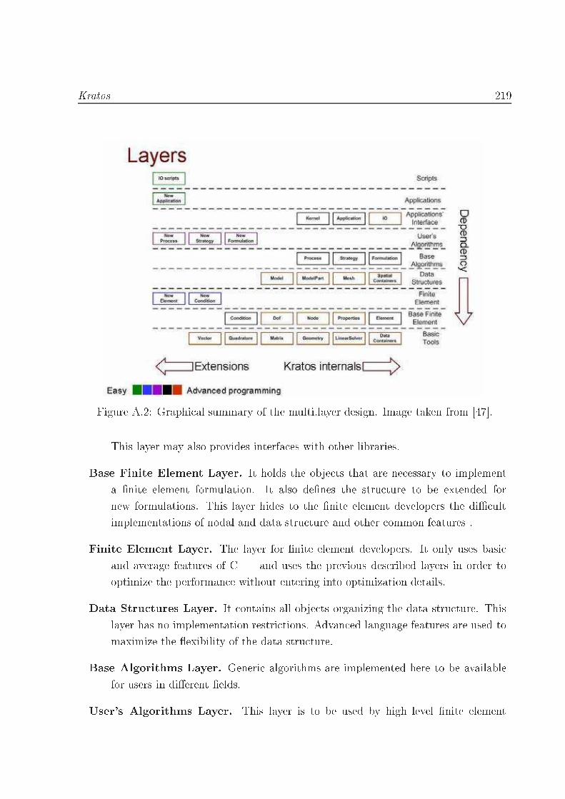
Kratos 219

Figure A.2: Graphi al summary of the multi.layer design. Image taken from [47.This layer may also provides interfa es with other libraries.Base Finite Element Layer. It holds the obje ts that are ne essary to implementa nite element formulation. It also denes the stru ture to be extended fornew formulations. This layer hides to the nite element developers the di ultimplementations of nodal and data stru ture and other ommon features .Finite Element Layer. The layer for nite element developers. It only uses basi and average features of C++ and uses the previous des ribed layers in order tooptimize the performan e without entering into optimization details.Data Stru tures Layer. It ontains all obje ts organizing the data stru ture. Thislayer has no implementation restri tions. Advan ed language features are used tomaximize the exibility of the data stru ture.Base Algorithms Layer. Generi algorithms are implemented here to be availablefor users in dierent elds.User's Algorithms Layer. This layer is to be used by high level nite element

220 Kratos Multiphysi sprogrammers. It ontains all lasses implementing the dierent algorithms inKratos.Appli ations' Interfa e Layer. It holds all the obje ts that manage Kratos and theirrelation with other appli ations. The omponents of this layer are implementedusing high level programming te hniques in order to provide the required exibility.Appli ations Layer. It ontains the interfa e of ertain appli ations with Kratos.S ripts Layer. Holds a set of IO s ripts whi h an be used to implement dierentalgorithms from outside Kratos. Pa kage users an use modules in this layer or reate their own extension without having knowledge of C++ programming or ofthe internal stru ture of Kratos. Via this layer they an a tivate and dea tivate ertain fun tionalities or implement a new global algorithm without entering intoKratos stru ture details.A graphi al representation of the stru ture an be seen in g. A.2A.1.3 Python interfa eKratos uses the fa ilities of Python language for IO data transmission [4. This exibleinterpreter with its obje t-oriented high level language an be used to implement andexe ute new algorithms using Kratos. Python allows an high level of exibility, withoutthe need of re ompiling the ode when debugging or testing new algorithms.A.2 GiD problem types and interfa esThe pre and post- pro essing is done using the in-house ommer ial sofware GiD [2.Dierent problem types have been developed in TCL to ustomize GiD insert the dataand print the results of the dierent appli ations presented in this work. They are allavailable in the kratos website [3.

Bibliography[1 Banqiao Dam. http://worldphoto olle tions.blogspot. om/2010/01/worlds-worst-ten-deadliest-natural.html.[2 GiD the Personal Pre and Post Pro essor. http://www.gidhome. om/.[3 Kratos, Multiphysi s opensour e fem ode. http://www. imne. om/kratos.[4 Python programming language. http://www.python.org/.[5 TetGen, A quality tethraedral mesh generator and three dimensional Delaunay.http://tetgen.berlios.de.[6 D.D. Adam and W.L. Wood. Comparison of hilber-hughes-taylor and bossak

α methods for the numeri al integration of vibration equations. InternationalJournal for Numeri al Methods in Engineering, 19:765771, 1983.[7 I. Akkerman, Y. Bazilevs, C. Kees, and M. Farthing. Isogeometri analysis offree-surfa e ow. Journal of Computational Physi s, 230:41374152, 2011.[8 A. Amiri and K. Vafai. Transient analysis of in ompressible ow through a pa kedbed. International Journal of Heat and Mass Transfer, 41:42594279, 1998.[9 I. Babuska. Finite element method with lagrangian multipliers. Numeris he Math-ematik, 20:179192, 1973.[10 J. Baiges. The Fixed-Mesh ALE method applied to multiphysi s problems usingstabilized formulations. PhD thesis: Universidad Politité ni a de Cataluña, 2010.[11 E. Barozzi and E. Gonzalez. Cal ulus Vol. I. Libreria Progetto Padova, 1996.

222 BIBLIOGRAPHY[12 J. Bear. Dynami s of uids in Pouros Media. Courier Dover Pubbli ations, 1988.[13 M.A. Biot. General theory of three dimensional onsolidation. Journal of AppliedPhysi s, 12:155164, 1941.[14 M.A. Biot. Theory of eleasti ity and onsolidation for a porous anisotropi solid.Journal of Applied Physi s, 26:182185, 1955.[15 R.B. Bird. Dynami s of polymeri liquids. John Wiley and Sons, 1987.[16 F. Brezzi. On the existen e, uniqueness and approximation of saddle point prob-lems araising from lagrange multipliers. Revue Française d'Automatique Informa-tique et Re her he Opérationalle, 8:129151, 1974.[17 A.N. Brooks and T.J.R. Huges. Streamline upwind/petrov-galerkin formulationsfor onve tion dominated ows with parti ular emphasis on the in ompressiblenavier-stokes equations. Computer Methods in Applied Ma hani s and Engineer-ing, 32:199259, 1982.[18 P. Bussetta, R. Boman, and J.P. Ponthot. Comparison of data transfer methodsbetween meshes in the frame of the abitrary lagrangian eulerian formalism. Pro- eeding of the V Internationa onferen e on Advan es Computational Methods inEngineering (ACOMEN 2011), -, 2011.[19 K. Butler, E. Oñate, S.R. Idelsohn, and R. Rossi. Modeling polymer melt owusing the parti le nite element method (pfem). Pro eeding of the Interam Con-feren e 2007, 2:929940, 2007.[20 N. Calvo. Genera ión de mallas tridimensionales por métodos duales. PhD thesis:Univesidad Na ional del Litoral, Argentina, 2005.[21 H. Campos, R. Morán, and M.A. Toledo. Estudio de la rotura de presas dematerial granular grueso uniforme no ohesivo sin elemento impermeable. fase deini io. Dam maintenan e and rehabilitation II, CRCpress Balkema, pages 599608,2010.[22 J.M. Carbonell. Modeling of ground exavation with the parti le element method.PhD thesis: Universidad Politité ni a de Cataluña, 2009.

BIBLIOGRAPHY 223[23 J.M. Carbonell, E. Oñate, and B.Suárez. Modeling of ground exavation with theparti le nite element method (pfem). ASCE: Journal of Engineering Me hani s,136:455463, 2008.[24 P.J. Carreau, D. Dekee, and R.P. Chhabra. Rheology of polymeri systems. Hansen,1997.[25 M. Cervera, M. Chiumenti, and R. Codina. Mixed stabilized nite element meth-ods in nonlinear solid me hani s. part i: Formulation. Computer Methods inApplied Me hani s and Engineering, 199:25592570, 2010.[26 M. Cervera, M. Chiumenti, and R. Codina. Mixed stabilized nite element meth-ods in nonlinear solid me hani s. part ii: Strain lo alization. Computer Methodsin Applied Me hani s and Engineering, 199:25712589, 2010.[27 M. Cervera, M. Chiumenti, and C. Agelet de Sara ibar. Softening, lo alizationand stabilization: apture of dis ontinuous solutions in j2 plasti ity. Interna-tional Journal for Numeri al and Analithi al Methods in Geome hani s, 28:373393, 2004.[28 M. Cervera, M. Chiumenti, and C. Angelet de Sara ibar. Shear band lo aliza-tion via lo al j2 ontinuum damage me hani s. Computer Methods in AppliedMe hani s and Engineering, 193:849880, 2004.[29 M. Cervera, M. Chiumenti, and Q. Valverde C. Agelet de Sara ibar. Mixed linear/-linear simpli ial elements for in ompressible elasti ity and plasti ity. ComputerMethods in Applied Ma hani s and Engineering, 192:52495263, 2003.[30 H. Chanson. Embankments overow prote tion system and earth dam spillways., hapter Chapter 4 of Dams: Impa ts, stability and design, pages 101132. NovaS ian e Publishers, In ., 2009.[31 R.P. Chhabra. Non-Newtonian Fluids: An Introdu tion, Rheology of ComplexFluids (Chapter 1). Springer, 2010.[32 M. Chiumenti, Q. Valverde, C. Agelet de Sara ibar, and M. Cervera. A stabilizedformulation for in ompressible plasti ity using linear triangles and tetrahedra.International Journal of Plasti ity, 20:14871504, 2004.

224 BIBLIOGRAPHY[33 A.J. Chorin. A numeri al method for solving in ompressible vis ous problems.Journal of Computational Physi s, 2:12, 1967.[34 R. Codina. A nodal-based implementation of a stabilized nite element methodfor in ompressible ow problems. International Journal for Numeri al Methods inFluids, 33:737.766, 2000.[35 R. Codina. On stabilized nite element methods for linear system of onve tion-diusion-rea tion equations. Computer Methods in Applied Ma hani s and Engi-neering, 188:6182, 2000.[36 R. Codina. Pressure stability in fra tional step nite element methods for in om-pressible ows. Journal of Computational Physi s, 170:112140, 2000.[37 R. Codina. Stabilization of in ompressibility and onve tion through orthogonalsub-s ales in nite element method. Computer Methods in Applied Ma hani s andEngineering, 190:15791599, 2000.[38 R. Codina. Stabilized nite element approximation of transient in ompressibleows using orthogonal subs ales. Computer Methods in Applied Me hani s andEngineering, 191:42954321, 2002.[39 R. Codina and A. Fol h. A stabilised nite element predi tor- orre tor s heme forthe in ompressible navier-stokes equations using a nodal-based implementation.International Journal for Numeri al Methods in Fluids, 44:483503, 2004.[40 R. Codina, G. Houzeaux, H. Coppola-Owen, and J. Baiges. The xed-mesh aleapproa h for the numeri al approximation of ows in moving domains. Journal ofComputational Physi s, 228:15911611, 2009.[41 R. Codina and O. Soto. Approximation of the in ompressible navier-stokesequations using orthogonal subs ale stabilization and pressure segregation onanisotropi nite element meshes. Computer Methods in Applied Ma hani s andEngineering, 193:14031419, 2004.[42 H. Coppola. A nite element model for free surfa e and two uid ows on xedmeshes. PhD thesis: Universidad Politité ni a de Cataluña, 2009.

BIBLIOGRAPHY 225[43 A.H. Coppola-Owen and R. Codina. Improving eulerian two-phase ow niteelement approximation with dis ontinuous gradient pressure shape fun tions. Int.J. Numer. Meth. Fluids, 49:1287.1304, 2005.[44 P. Coussot. Rheometry of pastes, suspensions and granular materials. Wiley andsons., 2005.[45 M. Cremonesi, L. Ferrara, A. Frangi, and U. Perego. Simulation of the ow offresh ement suspensions by a lagrangian nite element approa h. Journal ofNon-Newtonian Fluid Me hani s, 165:15551563, 2010.[46 M. Cremonesi, A. Frangi, and U. Perego. A lagrangian nite element approa h forthe simulation of water-waves indu ed by landslides. Computers and Stru tures,89:10861093, 2011.[47 P. Dadvand. A framework for developing nite element odes for multi-dis iplinaryappli ations. PhD thesis: Universidad Polité ni a de Cataluña, 2007.[48 P. Dadvand, R. Rossi, and E. Oñate. An obje t-oriented environment for devel-oping nite element odes for multi-dis iplinary appli ations. Ar hives of Compu-tational Methods in Engineering, 17:253297, 2010.[49 R de Boer. Theory of porous media. Springer-Verlag, Berlin, 2000.[50 L. Da Deppo, C. Datei, and P. Salandin. Sistemazione dei orsi d'a qua. LibreriaInternazionale Cortina (Padova), 2002.[51 J. Donea and A. Huerta. Finite Elements Methods for Flow Problems. Wiley,2003.[52 D. Dureisseix and H. Bavastrello. Information transfer between in ompatible niteelement meshes: appli ation to oupled thermo-vis oelasti ity. Computer Methodsin Applied Ma hani s and Engineering, 195:65236541, 2006.[53 E-DAMS. Numeri al and experimental te hniques for safety assessment and pro-te tion of embankment dams in overtopping s enarios. proje t of the National PlanR+D of the Spanish Ministry of S ien e and Innovation I+D BIA2010-21350-C03-00, 2010-2013.

226 BIBLIOGRAPHY[54 R. Elias and A. Coutinho. Stabilized edge-based nite element simulation of free-surfa e ows. Int. J. Numer. Meth. Fluids, 54:965993, 2007.[55 R. Elias, M. Martins, and A. Coutinho. Parallel edge-based solution of vis oplasti ows with the supg/pspg formulation. Computational Me hani s, 38:365381,2006. 10.1007/s00466-005-0012-y.[56 R.N. Elias, M.A.D. Martins, and L.G.A. Coutinho. Simple nite element-based omputation of distan e fun tions in unstru tured grids. International Journalfor Numeri al Methods Engineering, 72:10951110, 2007.[57 S. Ergun. Fluid ow through pa ked olumns. Chemi al Engineering Progress,48:8994, 1952.[58 A. Ghetti. Idrauli a. Ed. Cortina, 1984.[59 A.M. Grillet, B. Yang, and B. Khomamiand E.S.G. Shaqfeh. Modeling of vis- oelasti lid driven avity ow using nite element simulations. Journal of Non-Newtoninan Fluid Me hani s, 88:99131, 1999.[60 H.M. Hilber, T.J. Hughes, and R.L. Taylor. Improved numeri al dissipation fortime integration algorithms in stru tural dynami s. Earthquake Engineering andStru tural Dynami s, 5:283292, 1977.[61 T.J.R. Hughes. The nite element method. Linear stati and dynami nite ele-ment analysis. Englewood Clis, 1987.[62 T.J.R. Hughes. Multis ale phenomena: Green's fun tion, the diri hlet to neumannformulation, subgrid s ale models, bubbles and the origins of stabilized formula-tions. Computer Methods in Applied Ma hani s and Engineering, 127:387401,1995.[63 T.J.R. Hughes, L.P. Fran a, and G.M. Hulbert. A new nite element formula-tion for omputational uid dynami s: Viii. the galerkin/least-squares methodfor adve tive-diusive equations. Computer Methods in Applied Ma hani s andEngineering, 73:173189, 1989.[64 ICOLD. Bulletin 99, Dam Failures Statisti al Analysis. ICOLD, 1995.

BIBLIOGRAPHY 227[65 S. Idelsohn, M. Mier, and E. Oñate. Multi-uid ows with the parti le niteelement method. Computer Methods in Applied Me hani s and Engineering,198:27502767, 2009.[66 S. R. Idelsohn and E. Oñate. The hallenge of mass onservation in the solutionof free-surfa e ows with the fra tional-step method: Problems and solutions.International Journal for Numeri al Methods in Biomedi al Engineering,, 26:13131330, 2010.[67 S.R. Idelsohn, E. Oñate, and F. Del Pin. The parti le nite element method: apowerful tool to solve in ompressible ows with free-surfa es and breaking waves.International Journal for Numeri al Methods in Engineering., 61:964984, 2004.[68 S.R. Idelsohn, E. Oñate, F. Del Pin, and N. Calvo. Fluid-stru ture intera tionusing the parti le nite element method. Computer Methods in Applied Me hani sand Engineering, 195:21002123, 2006.[69 U. Israel. Implementation of an algorithm for data transfer on the uid stru -ture interfa e between non mat hing meshes in kratos and an algorithm for thegeneration of an interfa e between GiD and Kratos. Master thesis: Te hnis heUniversität Mün hen, 2006.[70 R. Juon and W.H. Hager. Flip bu ket with and without dee tors. Journal ofHydrauli Engineering, 126:837845, 2000.[71 C. Kees, I. Akkerman, M. Farthing, and Y. Bazilevs. A onservative level setmethod suitable for variable-order approximations and unstru tured meshes. Jour-nal of Computational Physi s, 230:45364558, 2011.[72 K.M.T. Kleesfman, G. Fekken, A.E.P. Veldman, B. Iwanowski, and B. Bu hner.A volume -of-uid based simulation method for wave impa t problems. Journalof Computational Physi s, 206:363393, 2005.[73 A. Larese, R. Rossi, and E. Oñate. Coupling eulerian and lagrangian models tosimulate seepage and evolution of failure in prototype ro kll dams. Pro eedingof the XI ICOLD Ben hmark Workshop on Numeri al Analysis of Dams, ISBN:978-84-695-1816-8, 2011.

228 BIBLIOGRAPHY[74 A. Larese, R. Rossi, and E. Oñate. Theme b: simulation of the behavior of proto-types of ro kll dams during overtopping s enarios: seepage evolution and begin-ning of failure. Pro eeding of the XI ICOLD Ben hmark Workshop on Numeri alAnalysis of Dams, ISBN: 978-84-695-1816-8, 2011.[75 A. Larese, R. Rossi, E. Oñate, and S.R. Idelsohn. Validation of the parti lenite element method (pfem) for simulation of free surfa e ows. EngineeringComputations, 25:385425, 2008.[76 C. Le huga, A. Lara, M. Berga, M. Viña, M.A. Toledo, R. Morán, H. Campos,J. Gar ía, and A. Larese. Estudios sobre el omportamiento de presas de es olleraante vertidos por orona ión. Proeeding for the IX Jornadas Españolas de presas.Valladolid, 2010.[77 S. Leliavsky. Design of dams for per olation and erosion. Hall UK, 1965.[78 R.L. Lewis and B.A. S hreer. The nite element method for the stati and dy-nami deformation and onsolidation of porous media. John Wiley and Sons,1998.[79 B. Li. Flowthrough and overtopped ro kll dams. PhD Thesis: University ofOttawa, 1995.[80 G. Lips omb and M. Denn. Flow of a bingham uid in omplex geometries. Journalof Non-Newtonian Fluid Me hani s, 14:337346, 1984.[81 R. Löhner. Applied omputational uid dynami s te hniques. Wiley, 2001.[82 J. Lubliner. Plasti ity Theory. Ma millan Publishing Company, New York, NY.,1990.[83 M. May. Implementation of a general algorithm for in ompressible and ompress-ible ows within the multi-physi s ode KRATOS and preparation of uid-stru ture oupling. Diploma thesis: Te hnis he Universität Mün hen, 2008.[84 M. Mier, S. Idelsohn, and E. Oñate. Advan es in the simulation of multi-uidows with the parti le nite element method. International Journal for Numeri alMethods in Fluids, 2010.

BIBLIOGRAPHY 229[85 E. Mitsoulis and Th. Zisis. Flow of bingham plasti s in a lid-driven square avity.Journal of Non-Newtonian Fluid Me hani s, 101:173180, 2001.[86 F. Mossaiby, R. Rossi, P. Dadvand, and S. Idelsohn. Open l-based implementa-tion of an unstru tured edge-based nite element onve tion-diusion solver ongraphi s hardware. International Journal for Numeri al Methods in Engineering,2011.[87 D.A. Nield and A. Bejan. Conve tion in porous media. Springer, 1992.[88 P. Nithiarasu, K.N. Seetharamu, and T. Sundararajan. Natural onve tive heattransfer in a uid saturated variable porosity medium. International Journal ofHeat and Mass Transfer, 40:39553967, 1997.[89 P. Nithiarasu, K. S. Sujatha, K. Ravindran, T. Sundararajan, and K. N.Seetharamu. Non-dar y natural onve tion in a hydrodynami ally and thermallyanisotropi porous medium. Computer Methods in Applied Me hani s and Engi-neering, 188:413430, 2000.[90 P. Nithiarasu, T. Sundararajan, and K. N. Seetharamu. Double-diusive natu-ral onve tion in a uid saturated porous avity with a freely onve ting wall.International Communi ations in Heat and Mass Transfer, 24:11211130, 1997.[91 O.Coussy. Me hani s of porous media. John Wiley and Sons, 1995.[92 E. Oñate. Derivation of stabilized equations for numeri al solution of adve tive-diusive transport and uid ow problems. Computer Methods in Applied Ma- hani s and Engineering, 151:233265, 1998.[93 E. Oñate. A stabilized nite element method for in ompressible vis ous ows usinga nite in rement al ulus formulation. Computer Methods in Applied Me hani sand Engineering, 182:355370, 2000.[94 E. Oñate, M.A. Celigueta, and S.R. Idelsohn. Modeling bed erosion in free surfa eows by the parti le nite element. A ta Geote hni a, 1:237252, 2006.[95 E. Oñate, M.A. Celigueta, S.R. Idelsohn, F. Salazar, and B. Suarez. Possibilitiesof the parti le nite element method for uid-soil-stru ture intera tion problems.Journal of Computational Me hani s, 48:307318, 2011.

230 BIBLIOGRAPHY[96 E. Oñate and J. Gar ía. A nite element method for uid stru ture intera tionwith surfa e waves using a nite al ulus formulation. Computer Methods in Ap-plied Me hani s and Engineering, 191:635660, 2001.[97 E. Oñate, J. Gar ía, S.R. Idelsohn, and F. Del Pin. Fi formulations for niteelement analysis of in ompressible ows. eulerian, ale and lagrangian approa hes.Computer Methods in Applied Me hani s and Engineering, 195:30013037, 2006.[98 E. Oñate, S.R. Idelsohn, M.A. Celigueta, and R. Rossi. Advan es in the parti le -nite element method for the analysis of uid multibody intera tion and bed erosionin free surfa e ows. Computer Methods in Applied Me hani s and Engineering,197:17771800, 2008.[99 E. Oñate, S.R. Idelsohn, M.A. Celigueta, R. Rossi, J. Marti, J.M. Carbonell,P. Ryzakov, and B. Suárez. Advan es in the parti le nite element method (PFEM)for solving oupled problems in engineering Book hapter: Parti le-Based Methods,Computational Methods in Applied S ien es., volume 25. E Oñate and R. Owen,2011.[100 E. Oñate, S.R. Idelsohn, F. Del Pin, and R. Aubry. The parti le nite elementmethod. an overview. International Journal of Computational Methods, 1:267307,2004.[101 E. Oñate, A. Valls, and J. Gar ía. Modeling in ompressible ows at low and highreynolds numbers via nite al ulus-nite element approa h. Journal of Compu-tational Physi s, 224:332351, 2007.[102 A. Orlando and D. Peri . Analysis of transfer pro edures in elastoplasti ity basedon the error in the onstitutive equations: theory and numeri al illustration. In-ternational Journal for Numeri al Methods in Engineering, 60:15951631, 2004.[103 S. Osher and R.P.Fedkiw. Level Set Methods and dynami impli it surfa es.Springer, 2003.[104 T. C. Papanastasiou. Flows of materials with yield. Journal of Rheology, 31:385404, 1987.[105 D. Peri¢ and S. Slijep evi¢. Computational modelling of vis oplasti uids basedon a stabilised nite element method. Engineering Computations, 18:577591,2001.

BIBLIOGRAPHY 231[106 J. Prin ipe. Subgrid s ale stabilized nite elements for low speed ows. PhD thesis:Universidad Politité ni a de Cataluña, 2008.[107 M. Que edo, M. Pastor, M.I. Herreros, and J.A. Fernandez Merodo. Numeri almodelling of the propagation of fast landslides using the nite element method.International Journal for Numeri al Methods in Engineering, 59:755794, 2004.[108 R. Rossi, A. Larese, P. Dadvand, and E: Oñate. An e ient edge-based level setnite element method for free surfa e ow problems. International Journal forNumeri al Methods in Fluids (DOI: 10.1002/d.3680), 2012.[109 P. Ryzhakov. Lagrangian FE methods for oupled problems in uid me hani s.PhD thesis: Universitat Polité ni a de Cataluña, 2010.[110 P. Ryzhakov, R. Rossi, S.R. Idelsohn, and E. Oñate. A monolithi lagrangianapproa h for uid-stru ture intera tion problems. International Journal of Com-putational Me hani s, 46-6:883899, 2010.[111 P. Ryzhakov, R. Rossi, and E. Oñate. An algorithm for the simulation of thermally oupled low speed ow problems. Int. Journal for Num. Methods in Fluids, 2011.[112 F. Salazar, R. Moran, R. Rossi, and A. Larese. Numeri al modeling of the hy-drauli performan e of oliana dam spillway using kratos. Pro eeding of the XIICOLD Ben hmark Workshop on Numeri al Analysis of Dams, Valen ia, ISBN:978-84-695-1816-8, 2011.[113 Hanan Samet. Foundations of Multidimensional and Metri Data Stru tures. Mor-gan Kaufmann, 2006.[114 J.A. Sethian. A fast mar hing level set method for monotoni ally advan ing fronts.Pro eedings of the National A ademy of S ien es, 93(4):15911595, 1995.[115 O. Soto, R. Lohner, J. Cebral, and F. Camelli. A stabilized edge-based impli itin ompressible ow formulation. Computer Methods in Applied Me hani s andEngineering, 193:21392154, 2004.[116 B. Moran T. Belyts hko, W. K. Liu. Nonlinear Finite Elements for Continua andStru tures. John Wiley and Sons, 2000.

232 BIBLIOGRAPHY[117 D.W. Taylor. Fundamentals of soil me hani s. John Wiley and Sons, New York,1948.[118 W. Taylor. Apli a iones de algoritmos que onservan la energía-momentum endinámi a no-lineal. Te hni al report, Publi a ión CIMNE n.259, 2004.[119 R. Temam. Sur l'approximation de la solution des équations de navier-stokes parla méthode des pas fra tionaires (i). Ar h. Ration. Me h. Anal, 32:135, 1969.[120 T.E. Tezduyar. Stabilized nite element formulations for in ompressible ow om-putations. Advan es in Applied Me hani s, 28:144, 1992.[121 T.E. Tezduyar, S. Shih, and S. Mittal. Time-a urate in ompressible ow om-putations with quadrilateral velo ity-pressure elements. University of Minnesota.Super omputer Institute Resear h Report USMI, 90:143, 1990.[122 M.A. Toledo. Presas De Es ollera Sometidas a Sobrevertido. Estudio delMovimientos dal Agua a Través de la Es ollera e de la Estabilidad Frente alDeslizamiento en Masa. PhD thesis: Universidad Polité ni a de Madrid, 1997.[123 M.A. Toledo. Safety of ro kll dams subje t to overtopping. Pro eding of theInternational Symposium on new Trend an guidelines on Dam Safety, 1998.[124 P. Vasseur, C.H. Wang, and M. Sen. Natural onve tion in an in lined re tangularporous slot: the brinkman-extended dar y model. ASME Journal of Heat Transfer,112:507511, 1990.[125 J.C. López Verdejo. Cara teriza ión del Pro eso de Satura ión de una Presa deEs ollera Meidiante Métodos Unidimensionales. Diploma de Estudios Avanzados:Universidad Polité ni a de Madrid, 2005.[126 W.L. Wood, M. Bossak, and O.C. Zienkiewi z. An alpha modi ation of new-mark's method. Int. J. for Num. Meth in Eng., 15:15621566, 1980.[127 XPRES. Desarrollo de un método para el estudio del pro eso de rotura de presasde es ollera por sobrevertido ombinando té ni as de elementos nitos y partí u-las. proje t of the National Plan R+D of the Spanish Ministry of S ien e andInnovation I+D BIA2007-68120-C03-01, 2007-2010.

BIBLIOGRAPHY 233[128 M. Zagonjolli. Dam Break Modelling, Risk Assessment and Un ertainty Analysisfor Flood Mitigation. PhD thsis: Delft University of Te hnology, 2007.[129 J. Zhang. An augmented lagrangian approa h to bingham uid ows in a lid-driven square avity with pie ewise linear equal-order nite elements. ComputerMethods in Applied Me hani s and Engineering, 199:3051 3057, 2010.[130 O.C. Zienkiewi z, A.H.C. Chan, M. Pastor, B.A. S hreer, and T. Shiomi. Com-putational Geome hani s with spe ial referen e to earthquake engineering. Wiley,1999.[131 O.C. Zienkiewi z and T. Shiomi. Dynami behaviour of saturated porous media:the generalised biot formulation and its numeri al solution. International JournalNum. Anal. Meth. Geome h., 8:7196, 1984.[132 O.C. Zienkiewi z, R.L. Taylor, and P. Nitharasu. Vol. 3. The nite elementmethod. Fluid dynami s. Elsevier, 2005.