Ann Oper Res (2014) 223:173–193DOI 10.1007/s10479-014-1619-1

A constraint programming-based approach to the crewscheduling problem of the Taipei mass rapid transitsystem

Anthony F. Han · Elvis C. Li

Published online: 30 May 2014© Springer Science+Business Media New York 2014

Abstract This paper addresses the crew scheduling problem for a mass rapid transit (MRT)system. The problem is to find a minimum number of duties to cover all tasks while satisfyingall the hard and soft scheduling rules. Such rules are complicated in real-world operationsand difficult to follow through optimization methods alone. In this paper, we propose aconstraint programming (CP)-based approach to solve the problem. The approach involvesa CP model for duty generation, a set covering problem model for duty optimization, andalternative ways to identify the final solution in different situations. We applied the proposedCP-based approach to solve a case problem for the Taipei MRT. Case application resultsusing real-world data showed that our approach is capable of reducing the number of dailyduties from 58 to 55 and achieving a 5.2 % savings in labor costs. We also incorporated thesoft rule considerations into the CP model in order to generate alternative optimum solutionsthat would improve the workload balance. The coefficient of variation of the work timedistribution improves significantly, falling from 21 % to approximately 5 %. Given the CPmodel’s comprehensive coverage of various scheduling rules, our proposed approach andmodels would also be applicable to other MRT systems.

Keywords Crew scheduling problem · Mass rapid transit · Constraint programming ·Set covering problem

1 Introduction

Crew scheduling is an important issue for crew management in public transportation systems.Crew management is concerned with building the rosters of crews needed to cover a planned

A. F. Han (B) · E. C. LiDepartment of Transportation Technology and Management,National Chiao Tung University, Hsinchu 30010, Taiwane-mail: afhan@mail.nctu.edu.tw

E. C. Lie-mail: zyun.tem94g@nctu.edu.tw

123

174 Ann Oper Res (2014) 223:173–193

timetable while satisfying operational and regulation rules. In practice, this complex andchallenging problem usually divides into crew scheduling and crew rostering (Caprara et al.1997). Crew scheduling aims to fulfill a minimum number of duties to cover all tasks withoutviolating any scheduling rules, such as break time requirements and maximum continuousdriving time limits. Based on the results of crew scheduling, crew rostering then generatesa roster that spans a given time period according to rostering rules (Yunes et al. 2005).Crew scheduling thus plays a critical role in assisting a transportation agency or companyin minimizing its labor costs. In this paper, we analyze the crew scheduling problem for theTaipei mass rapid transit (MRT) system and propose a constraint programming (CP)-basedapproach to solve the problem.

Crew scheduling problems have been applied to different transportation sectors includingairlines, bus transit, and the railway industry. Crew scheduling problems in the respectivesectors share many elements, such as the constraints imposed by rules and regulations, andthe need to cover all tasks while seeking to minimize labor costs. However, each applica-tion has its own unique characteristics and its own research challenges. Accordingly, mostcrew scheduling research focuses on a particular application area, rather than dealing with ageneral case (Ernst et al. 2004). In this paper, we focus on the crew scheduling problem forMRT systems. Good reviews of crew scheduling problems in other application areas include(Barnhart et al. 2003) for airlines, (Wilson 1999) for bus transit, and (Caprara et al. 1997) forrailways.

Existing studies on the crew scheduling problem for an MRT system basically considerthe problem as an optimization problem and propose approaches based on heuristic or meta-heuristic methods to solve the issue. For example, Chu and Chan (1998) proposed a three-stageheuristic method for solving the crew scheduling problem for the light rail transit system inHong Kong. Cavique et al. (1999) and Chew et al. (2001) applied tabu search metaheuristicsand presented cases on the Lisbon Underground and the Singapore MRT, respectively. Thesethree studies showed improvement over previous schedules. However, they fixed only twoor three pieces of work in each of the duties generated, and thus might limit the potentialfor obtaining better results. Park and Ryu (2006) employed a genetic algorithm with unex-pressed genes to solve a subway crew schedule, but the objective was to minimize uncoveredtasks rather than to minimize the labor costs. Elizondo et al. (2010) applied an evolutionaryalgorithm to solve crew scheduling for the Santiago Metro System, but they did not comparetheir results with actual schedules.

While existing literature on MRT applications relies mainly on metaheuristic methods,this paper presents a CP-based approach to tackle the crew scheduling problem of the TaipeiMRT. This approach consists of two phases: duty generation, which is actually a constraintsatisfaction problem,and duty optimization. Specifically, we propose the use of a CP model forduty generation and a set covering problem (SCP) model for duty optimization. Conventionalapproaches to tackle the MRT crew scheduling problem mainly take it as a constrainedoptimization problem in the structure of integer programming (IP). However, the numerousside constraints due to those scheduling rules tend to make the problem difficult to solve evenwith prevailing metaheuristics such as tabu search (Cavique et al. 1999) and evolutionaryalgorithms (Elizondo et al. 2010). On the other hand, the roots of CP can be traced back to thework in the field of artificial intelligence (AI) on solving constraint satisfaction problems in the1970s (Mackworth 1977). Because a constraint satisfaction problem may include constraintsin the form of logic implications, a CP system usually interleaves search and logical inferenceto find a feasible solution. Such inferences generally involve constraint propagation, whichpropagates the information contained in one constraint to the neighboring constraints, anddomain reduction, which reduces the range of variable domains that need to be traced, to

123

Ann Oper Res (2014) 223:173–193 175

expedite the search process (Lustig and Puget 2001). Brailsford et al. (1999) compared CAwith OR techniques and deemed that, for ease of implementation and flexibility, CP scoreshighly relative to most OR techniques. For computational time and solution quality, accordingto Puget (1995) the success of a CP approach critically depends on the amount of propagationthat the constraints permit. That is if the nature of a problem is such that a variable instantiationtriggers the pruning of many values from the domains of other variables, then CP is likelyto be successful. He argues that scheduling and timetabling problems are good candidatesfor CP. Therefore, it is reasonable for us to use CP to deal with the constraint satisfactionproblem confronted in the duty generation phase. Moreover, a good CP model also servesas an efficient column generator which facilitates solving a large-scale SCP which might beencountered in the duty optimization phase as discussed below.

Although a CP-based approach is new to MRT applications, it is not uncommon in otherapplication areas such as airlines (Fahle et al. 2002; Gabteni and Grönkvist 2009; Grönkvist2006) and bus transit systems (Silva 2001; Ftulis et al. 1998; Yunes et al. 2005). One advantageof CP is that it can express complex real-life constraints easily. Another advantage is thatit has the flexibility necessary to adopt changes in rules and to add new rules. Accordingly,a CP-based model for crew scheduling applications is more transferable to other cases thanconventional models purely based on heuristic or metaheuristic methods. In our proposedapproach, the CP model serves as a good tool for duty generation. Moreover, when theproblem scale of the SCP in the duty optimization phase is too large for the problem to besolved exactly, the CP model can be used to help solve the pricing sub-problem by generatingcolumns for the restricted SCP. Examples of how the CP-based column generation (CG)applies to airlines and bus systems were presented in Fahle et al. (2002) and Silva (2001),respectively. It has been found that the CP-based CG is more efficient than the MP-basedCG (Yunes et al. 2005). In recent years, CP has advanced significantly in many ways (Apt2003) and has been increasingly recognized as a powerful approach complimentary to ORmethods in solving combinatorial problems (Hentenryck 2002; Hooker 2006).

The remainder of this paper is organized as follows. In Sect. 2, we first define the crewscheduling problem for a general MRT system and then list all the operational and regulatoryrules and constraints that are most commonly seen in practice. We then propose the frameworkof a CP-based two-phase solution approach. In Sect. 3, we start with a brief description ofthe Taipei MRT and define the scope of the case problem as covering the Red–Orange line.This section also specifies the related data and parameters. Section 4 presents the modelingprocess for our case application. The decision variables, their domains, and all the constraintsof the CP model for duty generation are described in detail. In addition, this section presentsthe SCP model for duty optimization. Section 5 reports the case results in which we find thatour proposed methods can create 5 % savings in crew costs on the Red–Orange line. Thissection also shows how the CP model can be applied to improve the workload balance amongthe train drivers. Finally, Sect. 6 concludes the paper.

2 Problem description and CP-based solution framework

2.1 Problem description

When we refer to the crew of the MRT crew scheduling problem, we mean the operatorsor drivers of MRT trains. A full understanding of the MRT crew scheduling problem relieson the knowledge of the daily operation of the trains moving between MRT stations. Thestations of a typical MRT line can be classified into three categories. First are those stations

123

176 Ann Oper Res (2014) 223:173–193

that provide services primarily to MRT riders, meeting their requirements for boarding,alighting, transferring, and the like, but that do not provide services to the MRT trains fortheir parking and maintenance needs. For simplicity, these only-for-transit stations, if nototherwise specified, will be referred to as transit stations in the remainder of this paper.Second, terminal stations, or terminals, are those stations that not only serve riders but alsoprovide parking space and facilities for all the trains operated on the associated MRT line.Terminals are usually at the endpoints of an MRT line. Third, yard stations, or yards, are thosestations that are not open to serve the riders, but provide facilities and services exclusively forthe MRT trains for their maintenance and storage. A yard is usually located near a terminalstation. Because yards are not open for transit services, they are not shown on the MRT mapfor the general public. However, yard stations are essential to the daily operations of MRTtrains, and thus cannot be overlooked in the MRT crew scheduling problem. Figure 1 depictsa typical MRT line including the yard stations.

The daily operation of MRT trains can be divided into three periods or cycles: (1) publictransit service, (2) pre-transit operation, and (3) post-transit operation. The public transitservice cycle generally starts early in the morning and ends around midnight on the same day.Each trip of an MRT train operated in this cycle runs in a terminal-to-terminal pattern, runningfrom the origin terminal to the destination terminal and stopping at each of the intermediatestations; for example, the routes would be B–C–D–E–F and F–E–D–C–B for the line depictedin Fig. 1. The pre-transit operation cycle usually starts about 2 h before the public transitservice cycle. There are two operational functions involved in this cycle. The first is fordispatch-to-work, which requires a driver to move the MRT train from a yard to a terminalstation in preparation for the following operations originating from that terminal, e.g., A–Band G–F for the line in Fig. 1. The second is for track inspection, which also runs in a terminal-to-terminal pattern but without carrying any passengers on board the train. This inspectionoperation repeats several times before the start of daily transit service to ensure safety for thepublic. The post-transit operation cycle, which immediately follows the public transit servicecycle, involves dispatch-to-yard operations in which some of the empty trains are moved froma terminal station to a yard for required maintenance work scheduled that night, e.g., B–Aand F–G for the line in Fig. 1. The time periods, operational functions, and train trip patternsof the three cycles of the daily operation of an MRT system are summarized in Table 1.

The MRT crew scheduling problem is based on the set of tasks that must be performedwithin a given timetable for each line, as well as scheduling rules, with the goal of arriving ata minimum number of duties. Before presenting approaches and models to solve the problem,we need to describe the tasks, duties, and scheduling rules in more detail. A task representsthe minimum portion of work that can be assigned to a train operator and is derived fromtimetable and relief points (RP). The timetable, which lists all the work to be assigned to thecrew in a given day, contains departure and arrival times of all the trains for each station,including departure and arrival times to terminals and yards. RPs are those stations at which

Fig. 1 An MRT line with yardstations

123

Ann Oper Res (2014) 223:173–193 177

Table 1 Daily operation of MRT trains

Operational function Train trip pattern Approximate time period

Pre-transit cycle Dispatch-to-worktrack inspection

Yard-to-terminalterminal-to-terminal

4 am to 6 am

Public transit cycle Transit service Terminal-to-terminal 6 am to 12 pm

Post-transit cycle Dispatch-to-yard Terminal-to-yard 12 pm to 2 am

Fig. 2 Composition of a duty for MRT crew scheduling

the crew check-in and check-out for their daily duties and where they can relieve each other,rest, and dine. In general, the longer an MRT line is, the more RPs there are likely to be onthat line. While not all MRT stations can serve as RPs, both yards and terminal stations areusually RPs. In terms of transit stations, those in the middle of a long line are more likelyto be operated as RPs than others. The related data required to define a task thus include atrain number, a departure or origin RP station, a departure time, an arrival or destination RPstation, and an arrival time.

A duty consists of a sequence of tasks to be assigned to a single operator or driver for aday’s work. On any given day, the tasks assigned to a driver must be separated by breaks,because the driver needs to rest and dine during his or her shift. Moreover, deadhead trips (inwhich train operators are transported as passengers to another relief point) are an inevitablepart of a daily operation that best utilizes the workforce. Accordingly, the full contents of aduty include check-in, tasks, dining, rest, deadhead trips, and check-out. Figure 2 depicts anexample of a duty that consists of four tasks, two breaks including one for rest and one fordining, and one deadhead trip. In the figure, train icons denote the RP stations; the non-RPstations, though not shown, are included implicitly between each of the succeeding RP pairsdefined by a task or a deadhead trip.

Feasible duties for an MRT crew scheduling problem must satisfy all the operationalconstraints as well as regulatory and labor union rules. Scheduling rules are generally relatedto the time and/or location of the tasks involved in a single duty. The most common schedulingrules for an MRT system in general are described below.

(1) Location-related constraints

• Relief location fit. Each task must begin at the same RP where the previous taskended, or else a deadhead trip must be assigned to the duty. In a deadhead trip, a trainoperator is transported as a passenger to another relief point.

• Duty start-and-end location fit. The check-in and check-out of each duty must occurat the same RP, or else a deadhead trip must be assigned at the beginning or the endof the duty.

(2) Shift-related constraints

• Work shift rule. Due to the long hours of operation, an MRT system usually hasmultiple work shifts in a day for the crew to be able to cover all the tasks. Every dutyto be scheduled must start and finish during the same shift.

123

178 Ann Oper Res (2014) 223:173–193

• Number of meals in a shift. In most cases, the number of meals required in a full-timeshift is one. For graveyard and midnight shifts, however, the number is zero becauseof the long rest breaks already included in those shifts.

• Meal-time window constraint. For those shifts requiring a meal, the time for diningis restricted to a certain permissible period of time, and the dining can be assignedonly in that specific time window.

(3) Time-related constraints

• Rest-time limit. To allow the crew to have a reasonable amount of time to rest, thetime of each rest period assigned is restricted by a lower and upper bound.

• Meal-time limit. Similar to the rest-time limit, the amount of time allotted for eachmeal is restricted by a lower and upper bound.

• Continuous driving time limit. To prevent overexertion, the continuous driving time(CDT) in each duty cannot exceed an upper bound. Sometimes a lower bound forCDT is also used to avoid inefficient assignment of work.

All the scheduling constraints described above are also called hard rules, because they allmust be strictly satisfied in an MRT crew scheduling problem. In addition to these hard rules,the management may consider some soft rules. Soft rules generally represent issues that areof great concern but are difficult to capture explicitly in the problem formulation. A typicalexample of a soft rule for many MRT systems is the quest for workload balance. Anotherexample is the attempt to assign all duties in as few shifts as possible. Soft rules, althoughmore complicated than hard rules, can be handled by adding extra constraints or secondaryobjectives to the problem. While most of the MRT applications in the existing literature dealonly with the hard rules, our proposed CP-based approach attempts to tackle both the hardand the soft rules most commonly seen in an MRT system.

Table 2 compares the coverage of scheduling rules consider in our proposed CP modelwith that considered in other models developed for the MRT crew scheduling problems inthe cities of Hong Kong (Chu and Chan 1998), Lisbon of Portugal (Cavique et al. 1999),Singapore (Chew et al. 2001), Busan of Korea (Park and Ryu 2006), and Santiago of Chile(Elizondo et al. 2010). Only ours can cover all the scheduling rules listed in the table. Forexample, all the models except ours have overlooked the minimum and maximum rest timeconstraints and the number of meals requested in different shits. Moreover, while our modelputs no restrictions on the structure of a duty, all others restrict either the number of tasks,the number of shifts, or that of pieces of work in their models. This comprehensive coverageof scheduling rules suggests that our proposed approach has the potential to be applicable toMRT systems in different cities, not just the single case of Taipei presented in this paper.

2.2 CP-based solution framework

In this paper, we propose a CP-based approach to solve the MRT crew scheduling problem.Our proposed approach consists of two phases: duty generation and duty optimization. Inthe first phase, the problem of identifying feasible duties that satisfy all the hard rules forscheduling is actually a constraint satisfaction problem, rather than an optimization problem.Thus, based on the input data related to the tasks, shifts, and all the rules, we propose theformulation of a CP model to solve the associated constraint satisfaction problem. Dependingon the problem scale, the CP model may or may not be able to generate all the feasibleduties for crew scheduling. Nevertheless, in both cases the results of the CP model providevaluable input to the following phase of duty optimization. Note that, with appropriately

123

Ann Oper Res (2014) 223:173–193 179

Table 2 Comparison of crew scheduling rules considered in various MRT application studies

Ourapproach

Chu and Chan(1998)

Cavique etal. (1999)

Chew et al.(2001)

ParkandRyu(2006)

Elizondoet al.(2010)

Application city Taipei Hong Kong Lisbon Singapore Busan Santiago

Timetable coverage Yes Yes Yes Yes No Yes

Location fit

Relief point Yes Yes Yes Yes Yes Yes

Duty start-and-end Yes Yes Yes Yes Yes Yes

Rest time

Lower bound Yes No No No No No

Upper bound Yes No No No No No

Number of dining Yes No No No No No

Meal time

Time window Yes No Yes Yes No Noa

Lower bound Yes Yes Yesb Yes No No

Upper bound Yes No Yesb Yes No No

Continuous driving

Lower bound Yes Yes Yes No No No

Upper bound Yes Yes Yes Yes Yes Yes

Work time balance

Lower bound Yes No Yes No No No

Upper bound Yes No Yes No No Yes

Range of tasks

Full consideration Yes Noc Noc Noc Nod Yes

Work shifts

Full consideration Yes Yes Yes Yes Yes Noe

a The meal was always assigned to the break period following the maximum continuous driving timeb Both bounds were fixed to 1 hc Only two or three pieces of work were included in each dutyd This study fixed ten tasks in each dutye Only two full-time shifts were included in a day

added constraints, the CP model can consider soft rules in addition to all the hard rules. Laterin our case application, we will show how the soft rule of workload balance can be adoptedin our proposed CP model to improve the solution.

In the second phase of duty optimization, we formulate the problem as a SCP to findthe minimal cost in terms of a minimal number of duties that cover all the required tasks.However, the solution procedure involved in this phase is not straightforward. Depending onthe problem scale, we propose alternative ways to reach the minimum cost. When the CPmodel in phase one can generate all the feasible duties, we achieve a well-defined SCP inphase two. If the problem scale is not large, one can solve the SCP directly and obtain an exactoptimal solution. However, if the SCP is too large to solve, then it can be relaxed as a large-scale LP, and conventional CG techniques can be applied to solve the problem approximately(Desaulniers et al. 2005). On the other hand, if all the feasible duties cannot be generated inreasonable time by the CP model in phase one, we only obtain a partially defined SCP in phase

123

180 Ann Oper Res (2014) 223:173–193

Fig. 3 A solution framework for an MRT crew scheduling problem

two. In this case, both MP-based and CP-based CG procedures are applicable. We proposeapplying CP-based CG techniques to solve the SCP for duty optimization because it has beenfound that the CP-based CG is more efficient than the MP-based CG (Yunes et al. 2005).

The overall framework of our proposed CP-based solution approach for an MRT crewscheduling problem is shown in Fig. 3. The CP model plays a critical role in this solutionapproach. It not only serves as the core for duty generation in the first phase, but also providesan efficient tool to solve the pricing sub-problem for generating columns to the restricted SCPin the CP-based CG procedures for duty optimization. Since we have proposed different waysto solve the problems for different scenarios, this solution approach is applicable to MRTsystems of different scales. A successful application to the Taipei MRT is described next.

3 Case background and data description

3.1 Taipei MRT case background

Taipei is the capital city of the Republic of China, i.e., Taiwan. The Taipei MRT is thekey public transportation system servicing the city of Taipei and neighboring towns, with a

123

Ann Oper Res (2014) 223:173–193 181

Fig. 4 Taipei MRT network as of 2011

total population of approximately 5.5 million (Taipei City Government 2013). The system isTaiwan’s first MRT; the first line, the Muzha line, began operation in 1996. Currently, fivemain lines and three branch lines are in operation, with 89 stations and a total operationallength of approximately 101.9 km. The network of the Taipei MRT is shown in Fig. 4.The five main lines are the Brown line (Taipei Nangang Exhibition Center-Taipei Zoo), theRed–Green line (Danshui–Xindian), the Red–Orange line (Beitou–Nanshijiao), the Blue line(Taipei Nangang Exhibition Center–Yongning), and the Orange line (Luzhou–ZhongxiaoXinsheng); the three branch lines are the Pink line (Beitou–Xinbeitou) and the two Light

123

182 Ann Oper Res (2014) 223:173–193

Fig. 5 Number of trains in operation on a typical weekday on the Red–Orange line

Green lines (Qizhang–Xiaobitan and the C.K.S. Memorial Hall–Ximen Line). During June2013, the system carried an average of over 1.6 million passengers per day (Ticketing Centerof Station Operations Division 2013). Based on the current operations of the Taipei MRT,the crew schedule is managed on a line-by-line basis such that the crew members assignedto a specific line will not be assigned to other lines. In our case study, we address the crewscheduling problem for the Red–Orange (Beitou–Nanshijiao) line.

For the Red–Orange line, there are 20 stations in operation, and only Beitou and Nanshijiaoare RP stations. The yards on the line are Fuxinggang and Zhonghe, which is near Nanshijiao.The service period runs from 0530 to about 2400 every day, and the operational period fortrains runs from approximately 0430 to 0200 the next day. The average operational headwayis approximately 6 min in peak hours and 8 min in off-peak hours. However, the serviceheadway for transit riders is only about half of the operational headway, because the Red–Orange line overlaps heavily with the Red–Green line, as shown in Fig. 4. For MRT ridersboarding at the overlapping stations, the average service headway is approximately 3 min inpeak hours, and 4 min in off-peak hours. Figure 5 shows the number of trains in operationon the line for every half-hour period in a typical weekday. Generally, as seen in the figure,there are 13–19 trains in operation for most of the day, from 0530 to 2330. There is a totalnumber of 228 tasks derived from the requirements of daily operation.

3.2 Input data and parameters

In this section, we specify the input data and parameters required by our case study. Forconvenience, Table 3 gives a summary of the associated notations.

Most of the input data for the CP model are related to tasks or shifts. We use Task todenote the set of all the tasks, and T ask = {0, 1, 2, . . . , Nt}, where 0 is a dummy task andNt is the total number of train tasks (Nt = 228). For each task t ∈ T ask, the task is definedby five parameters: the train number (Numbert ), the origin RP station (Orgt ), the departuretime (Deptt ), the destination RP station (Dest ), and the arrival time (Arrt ). For each of thetrain tasks, these parameters are derived from a real operational timetable of the Red–Orangeline. On the other hand, for the dummy task, i.e., t = 0, we set a null value to its train numberand origin and destination stations, i.e., Number0 = Org0 = Des0 = 0, and a big number toits departure and arrival times, i.e., Arr0 = Dept0 = 9999, to facilitate our CP formulation.

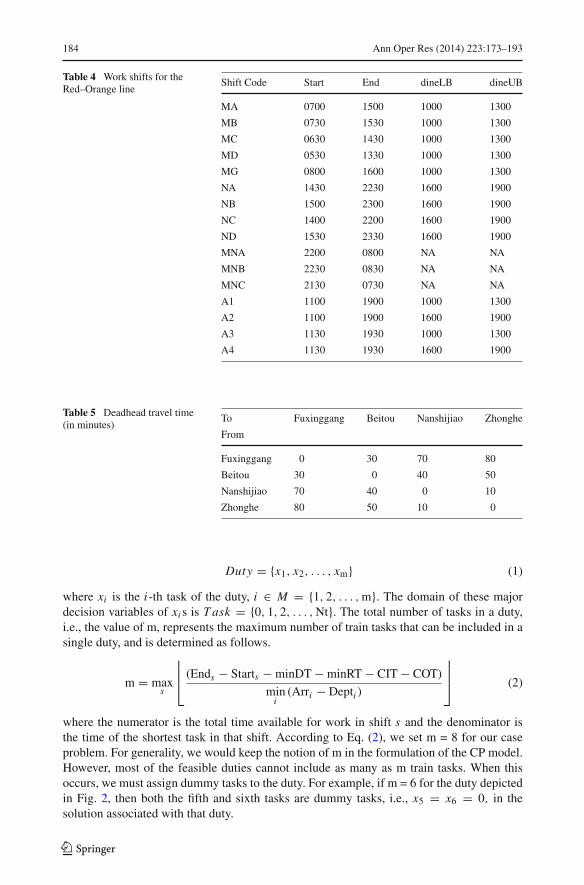
The management of the Taipei MRT runs the daily operation with 16 work shifts. Asdefined in Table 4, there are three graveyard shifts (MNA, MNB, and MNC), and 13 eight-hour full-time shifts which include five morning shifts (MA, MB, MC, MD and MG), fourafternoon shits (A1, A2, A3, and A4) and four night shifts (NA, NB, NC and ND). For each

123

Ann Oper Res (2014) 223:173–193 183

Table 3 The summary ofnotations of parameters and inputdata sets

Task The set of all tasks, T ask = {0, 1, 2, . . . , Nt}Nt Total number of train tasks

Numbert Train number of task t, ∀t ∈Task

Deptt Departure time of task t, ∀t ∈Task

Arrt Arrival time of task t, ∀t ∈ Task

Orgt Departure station of task t, ∀t ∈Task

Dest Arrival station of task t, ∀t ∈ Task

S The set of shifts (as defined in Table 4)

Starts Start time of shift s, ∀s ∈ S

Ends End time of shift s, ∀s ∈ S

dine_LBs The start of the meal-time window in shift s, ∀s ∈ S

dine_UBs The end of the meal-time window in shift s, ∀s ∈ S

maxRTs Maximal rest time allowed in shift s, ∀s ∈ S

numDines The number of dining required in shift s, ∀s ∈ S

minRT Minimal rest time

minDT Minimal meal time

maxDT Maximal meal time

CIT Check-in time

COT Check-out time

maxCDT Maximal continuous driving time

DHT (i, j) Deadhead travel time between relief point i and j

shift that requires a meal, the restricted time window for the meal is also given. For instance,when a train driver assigned to work in shift MG, which starts at 0800 and terminates at 1600,he or she must take a meal break between 1000 and 1300.

Other related data for our case study include the following:

• The check-in time (CIT) and check-out time (COT) are each 5 min.• The rest-time limit: the lower bound (minRT) is 15 min for all shifts and the upper bound

(maxRT) is 40 min for regular shifts and 270 min for the graveyard shifts.• The number of meals allowed (numDine) is 0 for the three graveyard shifts and 1 for all

the other shifts listed in Table 4.• The meal-time limit: the lower bound (minDT) and the upper bound (maxDT) are 30 and

50 min, respectively.• Continuous driving time limit: the lower bound (minCDT) and the upper bound (max-

CDT) are 45 and 180 min, respectively.• The deadhead travel times between all origin-destination pairs of RP stations are shown

in Table 5.

4 Modeling and case application

4.1 Decision variables of the CP model

In our solution approach, the CP model is designed for duty generation. Each solution obtainedfrom the CP model represents a feasible duty, and the duty can be defined as a sequence oftasks in the following way:

123

184 Ann Oper Res (2014) 223:173–193

Table 4 Work shifts for theRed–Orange line

Shift Code Start End dineLB dineUB

MA 0700 1500 1000 1300

MB 0730 1530 1000 1300

MC 0630 1430 1000 1300

MD 0530 1330 1000 1300

MG 0800 1600 1000 1300

NA 1430 2230 1600 1900

NB 1500 2300 1600 1900

NC 1400 2200 1600 1900

ND 1530 2330 1600 1900

MNA 2200 0800 NA NA

MNB 2230 0830 NA NA

MNC 2130 0730 NA NA

A1 1100 1900 1000 1300

A2 1100 1900 1600 1900

A3 1130 1930 1000 1300

A4 1130 1930 1600 1900

Table 5 Deadhead travel time(in minutes)

To Fuxinggang Beitou Nanshijiao Zhonghe

From

Fuxinggang 0 30 70 80

Beitou 30 0 40 50

Nanshijiao 70 40 0 10

Zhonghe 80 50 10 0

Duty = {x1, x2, . . . , xm} (1)

where xi is the i-th task of the duty, i ∈ M = {1, 2, . . . , m}. The domain of these majordecision variables of xi s is T ask = {0, 1, 2, . . . , Nt}. The total number of tasks in a duty,i.e., the value of m, represents the maximum number of train tasks that can be included in asingle duty, and is determined as follows.

m = maxs

⎢⎢⎢⎣

(Ends − Starts − minDT − minRT − CIT − COT)

mini

(Arri − Depti )

⎥⎥⎥⎦ (2)

where the numerator is the total time available for work in shift s and the denominator isthe time of the shortest task in that shift. According to Eq. (2), we set m = 8 for our caseproblem. For generality, we would keep the notion of m in the formulation of the CP model.However, most of the feasible duties cannot include as many as m train tasks. When thisoccurs, we must assign dummy tasks to the duty. For example, if m = 6 for the duty depictedin Fig. 2, then both the fifth and sixth tasks are dummy tasks, i.e., x5 = x6 = 0, in thesolution associated with that duty.

123

Ann Oper Res (2014) 223:173–193 185

Between two tasks there may be a break for a rest or a meal. The break variable betweentwo adjacent tasks of i and i +1, break(xi , xi+1), is a binary variable. When the two tasks arenot consecutive and the latter is not a dummy task, the break variable is equal to 1; otherwise,the variable is 0. The break variable is defined as follows:

break(xi , xi+1) ={

1 if Arrxi �= Deptxi+1∧ xi+1 �= 0

0 otherwisefor i = 1, 2, . . . , m − 1 (3)

When a break occurs, it must be designated as taking either a rest or a meal. Accordingly, weneed to define two more binary or indicator variables for dining(xi , xi+1) and rest (xi , xi+1)

as the following.

break(xi , xi+1) = dining(xi , xi+1) + rest (xi , xi+1) for i = 1, 2, . . . , m − 1 (4)

In addition to the break variable, we define an intermediate variable, breaktime(xi , xi+1),to trace the duration of the break between xi and xi+1, as shown in Eq. (5).

breaktime(xi , xi+1)={

Deptxi+1−Arrxi −DHT(Desxi

, Orgxi+1) if break(xi , xi+1) = 1

0 otherwisefor i = 1, 2, . . . , m − 1

(5)

Here, Deptxi+1−Arrxi is the time gap between the two adjacent tasks, and DHT(Desxi

, Orgxi+1)

is the deadhead travel time between the two stations Desxi and Orgxi+1. If the two stations

are the same, then DHT(Desxi, Orgxi+1

) is null, and the break time will simply be the timegap of Deptxi+1

− Arrxi ; otherwise, the deadhead travel time between the two stations mustbe subtracted from the break time.

Note that Eqs. (3) through (5) apply for i = 1, 2, . . . , m − 1, but not for i = m. This isbecause no further breaks can follow the very last task xm in a duty as defined in Eq. (1).

The continuous driving time is another important variable in our CP model. We denoteC DTi as the cumulative CDT variable at the end of task i , and it counts only for the last taskm and those tasks that end with a break. In transit scheduling, a piece of work, or a workpiece, is a sequence of consecutive tasks without breaks. Therefore, for the last task of eachwork piece, the CDT variable has to keep track of the continuous driving time for all the tasksinvolved in that specific work piece. However, the accumulation of driving time starts withthe same first task for all work pieces. Double counting in the accumulation process must beavoided. The CDT variables are thus defined as the following:

CDTi ={∑i

n=1 (Arrxn − Deptxn) − ∑i−1

k=1 C DTk if Arrxi �= Deptxi+1

0 otherwisefor i = 1, 2, . . . , m − 1

(6)

and

CDTm =m

∑

n=1

(Arrxn − Deptxn) −

m−1∑

k=1

CDTk (7)

As an example, there are three work pieces: (x1 − x2), (x3), and (x4) for the duty shown inFig. 2; only CDT2, CDT3, and CDT4 have meaningful nonzero values, and the CDTi s for allother tasks are null. Table 6 summarizes the variables and their associated domains definedin our CP model.

As mentioned in Sect. 2.1, the CDT of a feasible duty cannot exceed the upper bound ofmaxCDT. This can be easily handled by taking the upper bound into the definition of thevariable’s domain. Specifically, we set maxCDT as the upper bound of the finite domain of

123

186 Ann Oper Res (2014) 223:173–193

Table 6 The variables and their domains

Variables Description Domain

xi i-th task in the solution of a duty T ask = {0, 1, 2, . . . , Nt} , ∀i ∈ M

break(xi , xi+1) indicator of the break between xi andxi+1

{0, 1} , for i = 1, 2, . . . , m − 1

breaktime(xi , xi+1) the time length of the break between xiand xi+1

{0, 1, . . . , 999} , for i = 1, 2, . . . , m − 1

dining(xi , xi+1) indicator of the dining between xi andxi+1

{0, 1} , for i = 1, 2, . . . , m − 1

rest(xi , xi+1) indicator of the rest between xi and xi+1 {0, 1} , for i = 1, 2, . . . , m − 1

CDTi the continuous driving time at the end oftask i

{0, 1, . . . , maxCDT} ,∀i ∈ M

the set variable CDTi for every i ∈ M . However, the lower bound of the CDT time, i.e.,minCDT, cannot be treated similarly because the CDTi as defined in Eq. (6) is always zerofor those tasks not followed by breaks. Accordingly, the minCDT must be considered in theconstraints as described in the following section.

4.2 Constraints and CP-based duty generation

Feasible duties must satisfy the scheduling rules described in Sect. 2.1. All those rules,except the timetable coverage constraint which will be considered in the next phase of dutyoptimization, are covered in the CP model. Before presenting the constraints for meetingthe scheduling rules, we first propose Eq. (8) to ensure the appropriate order of the taskscontained in each duty.

Deptxi+1≥ Arrxi for i = 1, 2, . . . , m − 1 (8)

For simplicity, the constraints formulated in the CP model will also be referred to as equationsin this paper.

Considering the location fit of the RP stations, we can trace the train that connects twoconsecutive tasks at the same station. Thus, this location fit rule can be formulated as:

Arrxi = Deptxi+1⇒ numberxi = numberxi+1 for i = 1, 2, . . . , m − 1 (9)

The work shift rule requires that all the tasks in a feasible duty must start and end withina time period of [Starts + CIT, Ends−COT], which takes into account both the check-in andcheck-out time for the duty. However, this does not apply for dummy tasks. Therefore, wewrite two constraints to define the work shift rule as follows.

xi �= 0 ⇒ Deptxi≥ Starts + CIT ∀i ∈ M and s ∈ S (10)

xi �= 0 ⇒ Arrxi ≤ Ends − COT − DHT(Desxi , Orgx1) ∀i ∈ M and s ∈ S (11)

Eqs. (10) and (11) restrict, respectively, the start and end of each non-dummy train task to theright time limit. While the former is clear, the latter is bit complicated because it also servesas a location fit constraint. In addition to the time limit, Eq. (11) also considers whether theend station Desxi of a non-dummy task, xi , is the same as the station where the duty starts,i.e., Orgx1

. If these two stations are not the same, then we must reserve a deadhead trip of timeDHT(Desxi

, Orgx1) for dispatching the driver back to Orgx1

to ensure the duty start-and-endlocation fit as described in Sect. 2.1.

123

Ann Oper Res (2014) 223:173–193 187

Fig. 6 Duty generation using aCP model

Eqs. (12) and (13) define the time limit constraint for rest and dining respectively. Forboth types of breaks, the break time must follow its associated time limits. Moreover, Eq.(13) not only constrains the meal time to its bounds of minDT and maxDT, but also stipulatesthat the meal time must be assigned in the period of [dine_LB, dine_UB].

rest(xi , xi+1) = 1 ⇒ minRT ≤ breaktime(xi , xi+1) ≤ maxRTs

for i = 1, 2, . . . , m − 1 and s ∈ S (12)

dining(xi , xi+1) = 1 ⇒ minDT ≤ breaktime(xi , xi+1) ≤ maxDT ∧dine_LBs ≤ Arrxi ≤ dine_UBs for i = 1, 2, . . . , m − 1 and s ∈ S

(13)

For the dining breaks, Eq. (14) demands that the number of meals in a shift must follow thepre-set numDine.

m−1∑

i=1

dining(xi , xi+1) = numDines ∀s ∈ S (14)

Finally, for the continuous driving time constraint, we need consider only the lower bound(minCDT) in our constraints, because the upper bound (maxCDT) has been adopted in thedomain of the CDTi variables as defined in Eqs. (6) and (7). And we can easily use the CDTi

variables to define this constraint as the following.

Arrxi �= Deptxi+1⇒ C DTi ≥ minCDT for i = 1, 2, . . . , m−1 (15)

xm �= 0 ⇒ C DTm ≥ minCDT (16)

Our proposed CP model includes both the variables and constraints defined in this andprevious sections. For duty generation in our case problem, we use the ILOG OPL Studio 3.7.1(ILOG 2003) to solve the CP model. For each work shift, the feasible duties are generatedone by one by solving the CP model; the procedure repeats itself until no more solutions orthe feasible duties can be found, or a pre-determined computer time has expired. The wholeduty generation process stops when the CP model has been solved for all the shifts. Figure 6summarizes the duty generation process based on the CP model we proposed.

4.3 SCP model and duty optimization

Given all the feasible duties generated from the CP model, the final stage of the solutionprocess is to find the minimum number of duties that will satisfy all the MRT scheduling

123

188 Ann Oper Res (2014) 223:173–193

rules. This duty optimization problem is formulated as the following SCP model.

Min∑

j∈F D

Duty j (17)

subject to∑

j∈F D

ai j Duty j ≥ 1 ∀i ∈ Task (18)

Duty j ∈ {0, 1} ∀ j ∈ FD (19)

whereTask is the set of tasks as given in the CP model, andFD is the set of all feasible duties obtained from the CP model,

ai j ={

1 if task i is included in duty j0 otherwise

∀i ∈ T ask, j ∈ FD

As shown in the objective (17), the SCP model assumes the same unity cost for all the dutiesand seeks to minimize the total number of duties to be selected. The constraint (18) requiresthat each task i be covered by at least one of the duties in the solution. The constraint (19)simply defines the binary variable of the problem.

When the CP model in the previous stage is capable of generating the full set of FD, wecan either solve the SCP directly or tackle it with conventional column generation techniques.On the other hand, when the CP model cannot generate all the feasible duties, we propose theadoption of a CP-based column generation approach, as mentioned in Sect. 2.2. A genericversion of CP-based CG solution procedures proceeds as follows. First, we solve the restrictedmaster SCP as an LP and obtain the reduced cost π for each task to be covered. Second,we add two constraints to the CP model and use the modified CP model as the engine forgenerating new columns of feasible duties. Each new duty must (1) be different from theexisting duties in FD, and (2) have a negative reduced cost, i.e., rc = 1− ∑

i∈m πxi < 0.Third, we include the new columns in the restricted master SCP and repeat the process untilno more duties can be generated by the modified CP model. Finally, we have to convertthe solutions into binary variables to obtain an approximate solution. More sophisticatedCP-based CG techniques can be found in Silva (2001) and Yunes et al. (2005).

5 Results

5.1 Primary results of the case problem

We coded the CP and the SCP models in OPL (Hentenryck 1999), and also coded the wholesolution process in the OPL scripting language to integrate the implementation of both modelson the ILOG OPL Studio 3.7.1 platform (ILOG 2003). The whole solution process was carriedout on an AMD 64 3000+ personal computer with 1 GB RAM in a Windows XP professionalenvironment. Our proposed CP model did generate all the feasible duties in the first phaseof duty generation, so there was no need for us to invoke a CP-based column generationprocedure to solve our case problem. Moreover, due to the moderate scale of the SCP in ourcase, i.e., 56,562 feasible duties in total, the problem in the second phase for duty optimizationwas able to be solved to its integer solution on the ILOG OPL Studio 3.7.1 platform. Thisimplies that our approach can solve the problem to its exact solution for those MRT lines

123

Ann Oper Res (2014) 223:173–193 189

Table 7 Results of the case problem of the Red–Orange line in the Taipei MRT

Total solutiontime

# Dutiesscheduled

# Shiftsadopted

Total work time, TWT

Avg. (min) SD (min) CV (%)

Taipei MRT 1 week 58 14 320.7 67.4 21.0

CP-based approach ∼5 min (307”) 55 11 351.1 38.2 10.9

which have a scale similar to the Red–Orange line in Taipei. And only when applying thisCP-based approach to an MRT line whose scale is larger than the Red–Orange line, theCP-based column generation procedure may be required to facilitate the solution process.Table 7 summarizes the results of our case application.

In the Taipei MRT, the crew schedule is generated manually by an experienced person.While the manual results provided by the Taipei MRT required 58 duties for weekday oper-ation, our approach generated a solution of 55 duties. This generates approximately 5.2 %savings in labor costs for the Red–Orange line of the Taipei MRT. Our results have othermerits beyond cost savings, as well. Our results can satisfy all the scheduling rules used bythe Taipei MRT, while the manual results cannot fully meet the rest and dining-time require-ments. Moreover, our results can make daily operations easier to manage, with 11 work shiftsrather than the current 14 shifts.

The computer implementation of our solution is efficient. While the manual process usu-ally takes a week, our approach takes only 307 s, i.e., approximately 5 min, to generate allthe results. Specifically, the CP model implementation took 113 s to generate all the 56,562feasible duties in the 16 shifts considered. And the optimal solution of the SCP took 194s. As MRT crew scheduling is a planning-oriented problem, the computer efficiency of ourproposed models should be adequate for real-world applications.

As mentioned earlier in Sect. 2.1, workload balance in general is a big concern in themanagement of an MRT system. In practice, workload balance does not consider the dutiesassigned in graveyard shifts because of the different nature of the work involved. For eachof the duties in a regular or non-graveyard shift in the Taipei MRT, the workload is definedby the total work time (TWT), which includes the time of both train tasks and deadheadtrips assigned in the duty. There are 14 graveyard-shift duties in both the manual resultsprovided by the Taipei MRT and our results, so the numbers of regular-shift duties are 44and 41, respectively. For such duties, the average value and standard deviation of the TWTare illustrated in Table 7. To evaluate the workload balance, the coefficient of variation (CV),which is the mean divided by the standard deviation, of the TWT is a reasonable performancemeasure. As shown in the table, the CV of the TWT reduces almost to half, from 21.0 to10.9 %, with our improvement. It implies that even without soft rules, the CP-based approachcan be effective in improving the workload balance. In fact, our CP model, described next,can further improve the workload balance.

5.2 Extended results with soft rule considerations

Our proposed CP model can be easily extended to consider the soft rule of seeking workloadbalance. The main idea is to expand the CP model with several additional constraints togovern the TWT in a more reasonable range so as to achieve a better workload balance. First,we define the TWT of a duty by the following three constraints (20), (21), and (22), and addthem into our CP model.

123

190 Ann Oper Res (2014) 223:173–193

Table 8 Alternative optimum solutions with soft-rule considerations

[minTWT,maxTWT]

# Dutiesscheduled

# Shiftsadopted

CV ofTWT (%)

# Feasibleduties

Total CPU time (s) (CP, SCP)

None 55 11 10.9 56562 307 (113, 194)

[300, 400] 55 10 7.5 37101 285.85 (99.55, 186.3)

[320, 400] 55 11 6.7 23742 159.8 (86.8, 73)

[340, 400] 55 11 4.8 16159 129.53 (80.2, 49.33)

[300, 380] 55 10 5.3 36208 259.95 (98.9, 161.05)

T W T =lst∑

j=1(Arrx j − Deptx j

) +lst−1∑

j=1DHT(Desx j , Orgx j+1

) + DHT(Desxlst , Orgx1)

(20)

where lst denotes the last train task of the duty and is determined by

xi �= 0 ∧ xi+1 = 0 ⇒ lst = i for i = 1, 2, . . . , m − 1 (21)

xm �= 0 ⇒ lst = m (22)

Moreover, we add in the fourth constraint (23) to restrict the TWT in the range of [minTWT,maxTWT], where minTWT and maxTWT represent the bounds of the time range.

minTWTs ≤ T W T ≤ maxTWT for s /∈ {MNA, MNB, MNC} (23)

Based on the results of the average and standard deviation of the TWT of the first solutionshown in Table 7, we have considered three values, 300, 320, and 340, for minTWT, andtwo values, 380 and 400, for maxTWT. Using these parameters, we run the expanded CPmodel with different settings for the TWT bounds and then obtain the optimal solution fromthe subsequent SCP model. Finally, we found four alternative minimum-cost solutions withthe same minimum cost of 55 duties but with different degrees of workload balance. Table 8summarizes these results. As compared with the first solution without TWT bounds, the CVof the TWT again can be significantly reduced, from 10.9 % to as low as 4.8 %.

However, the slight difference in the CV values among the alternative solutions is insuf-ficient to identify the most desirable solution. To overcome this obstacle, we plot the barcharts of the work time distribution for the base case, with the first solution and the fouralternative solutions depicted in Fig. 7 for comparison. This figure, together with Table 8,can provide valuable information for a decision maker who has in mind the soft-rule consid-erations of workload balance and minimum work shifts. One can easily observe from Fig. 7ethat, although this solution has the lowest CV value of 4.8 %, its TWT distribution is not asevenly distributed as that of the solutions depicted in Fig. 7c, d and f. On the other hand, theTWT distribution of the solution with TWT bounds of [300, 380], as shown in Fig. 7f, looksquite attractive. It exhibits a narrow and rather symmetric bell-shaped distribution of TWTthat has not been seen in other comparable solutions. Moreover, for work shifts, this solutionrequires a minimum number of 10 shifts to work with.

Note that, as shown in Table 8, the solution time for solving for alternative solutionswith TWT bounds is even less than that for the first solution. The solution time is reducedsignificantly from 307 s to as low as 130 s. This shows another merit of a CP model, i.e., withproperly designed additional constraints the model can be solved more efficiently. Similar

123

Ann Oper Res (2014) 223:173–193 191

Fig

.7W

ork

time

dist

ribu

tion

ofal

tern

ativ

eso

lutio

ns

123

192 Ann Oper Res (2014) 223:173–193

results can be found in Goumopoulos and Housos (2004) in the context of their applicationsto airline crew scheduling problems.

6 Conclusions

In this paper, we proposed a CP-based approach to solve the crew scheduling problem forMRT operations. Existing studies on MRT crew scheduling applications consider the problemas primarily an optimization problem and solve the problem using heuristic or metaheuristicmethods. Our paper seems to be one of the first in the literature that applies CP models toMRT crew scheduling applications.

We applied the CP-based approach to tackle the crew scheduling problem for the Red–Orange line of the Taipei MRT and found encouraging results. As compared with the manualresults generated by the Taipei MRT, which barely meet rest and dining-time constraints, ourresults can reduce the number of duties required in the daily operation from 58 to 55, whichrepresents an approximate savings of 5.2 % in labor costs. Moreover, the number of workshifts required reduces from 14 to 11, and the workload balance, in terms of the coefficientof variation of the total work time distribution, improves significantly, from 21 to 11 %.

The proposed CP model also allows the flexibility to accommodate soft-rule considera-tions. In this paper, we demonstrated how to incorporate the workload balance considerationinto the CP-based solution process and easily generate four alternative optimum solutionswith better workload balance performance. With the same minimum cost of 55 duties, thecoefficient of variation of the total work time distribution further improves from 11 % toapproximately 5 %.

In our study, we have considered a comprehensive coverage of the scheduling rules mostcommonly seen in practice. Thus, the proposed CP-based approach and models may havethe potential for application to MRT systems in cities other than Taipei.

References

Apt, K. R. (2003). Pricinples of constraint programming. Cambridge: Cambridge University Press.Barnhart, C., Cohn, A., Johnson, E., Klabjan, D., Nemhauser, G., & Vance, P. (2003). Airline crew scheduling.

In R. W. Hall (Ed.), Handbook of transportation science (Vol. 56, pp. 517–560). New York: Springer.Brailsford, S. C., Potts, C. N., & Smith, B. M. (1999). Constraint satisfaction problems: Algorithms and

applications. European Journal of Operational Research, 119(3), 557–581.Caprara, A., Fischetti, M., Toth, P., Vigo, D., & Guida, P. L. (1997). Algorithms for railway crew management.

Mathematical Programming, 79(1–3), 125–141.Cavique, I., Rego, C., & Themido, I. (1999). Subgraph ejection chains and tabu search for the crew scheduling

problem. Journal of the Operational Research Society, 50(6), 608–616.Chew, K. L., Pang, J., Liu, Q. Z., Ou, J. H., & Teo, C. P. (2001). An optimization based approach to the train

operator scheduling problem at Singapore MRT. Annals of Operations Research, 108(1), 111–122.Chu, S. C. K., & Chan, E. C. H. (1998). Crew scheduling of light rail transit in Hong Kong: From modeling

to implementation. Computers Operations Research, 25(11), 887–894.de Silva, A. (2001). Combining constraint programming and linear programming on an example of bus driver

scheduling. Annals of Operations Research, 108(1), 277–291.Desaulniers, G., Desrosiers, J., & Solomon, M. M. (2005). Column generation. New York: Springer.Elizondo, R., Parada, V., Pradenas, L., & Artigues, C. (2010). An evolutionary and constructive approach to

a crew scheduling problem in underground passenger transport. Journal of Heuristics, 16(4), 575–591.Ernst, A. T., Jiang, H., Krishnamoorthy, M., & Sier, D. (2004). Staff scheduling and rostering: A review of

applications, methods and models. European Journal of Operational Research, 153(1), 3–27.Fahle, T., Junker, U., Karisch, S. E., Kohl, N., Sellmann, M., & Vaaben, B. (2002). Constraint programming

based column generation for crew assignment. Journal of Heuristics, 30(1), 59–81.

123

Ann Oper Res (2014) 223:173–193 193

Ftulis, S. G., Giordano, M., Pluss, J. J., & Vota, R. J. (1998). Rule-based constraints programming: Applicationto crew assignment. Expert Systems With Applications, 15(1), 77–85.

Gabteni, S., & Grönkvist, M. (2009). Combining column generation and constraint programming to solve thetail assignment problem. Annals of Operations Research, 171(1), 61–76.

Goumopoulos, C., & Housos, E. (2004). Efficient trip generation with a rule modeling system for crewscheduling problems. Journal of Systems and Software, 69(1–2), 43–56.

Grönkvist, M. (2006). Accelerating column generation for aircraft scheduling using constraint propagation.Computers and Operations Research, 33(10), 2918–2934.

Hooker, J. N. (2006). Operations research methods in constraint programming. In F. Rossi, et al. (Eds.),Handbook of constraint programming (pp. 527–570). Amsterdam: Elsevier.

ILOG. (2003). ILOG OPL Studio 3.7 Studio user’s manual. SA: ILOG.Lustig, I. J., & Puget, J. F. (2001). Program does not equal program: Constraint programming and its relationship

to mathematical programming. Interfaces, 31(6), 29–53.Mackworth, A. K. (1977). Consistency in networks with relations. Artificial Intelligence, 8(1), 99–118.Park, T., & Ryu, K. R. (2006). Crew pairing optimization by a genetic algorithm with unexpressed genes.

Journal of Intelligent Manufacturing, 17(4), 375–383.Puget, J. F. (1995). A comparison between constraint programming and integer programming. In Proceedings

of the Conference on Applied Mathematical Programming and Modelling (APMOD95). Uxbridge: BrunelUniversity

Taipei City Government, Department of Civil Affairs. (2013). Statistics in population and each districthouseholds in Taipei city July-2013. Retrieved August 2, 2013, from http://www.ca.taipei.gov.tw/public/Attachment/3829432175.xls

Ticketing Center of Station Operations Division. (2013). Transport volume statistics: June-2013. Resourcedocument. Taipei Rapid Transit Corporation. Retrieved July 5, 2013 from http://web.trtc.com.tw/RidershipCounts/E/10206e.htm

Van Hentenryck, P. (1999). The OPL optimization programming language. Combridge, MA: MIT Press.Van Hentenryck, P. (2002). Constraint and integer programming in OPL. Journal on Computing, 14(4), 345–

372.Wilson, N. H. M. (1999). Computer-aided transit scheduling (Vol. 471). Berlin: Springer.Yunes, T. H., Moura, A. V., & de Souza, C. C. (2005). Hybrid column generation approaches for urban transit

crew management problems. Transportation Science, 39(2), 273–288.

123