571

Evaluating StatisticsIn our day-to-day experience all of us encounter arguments that rest on statistical evidence. An especially prolifi c source of such arguments is the advertising indus-try. We are constantly told that we ought to sign up with a certain cell phone service because it has 30 percent fewer dropped calls, buy a certain kind of car because it gets 5 percent better gas mileage, and use a certain cold remedy because it is recommended by four out of fi ve physicians. But the advertising industry is not the only source. We oft en read in the newspapers that some union is asking an increase in pay because its members earn less than the average or that a certain region is threatened with fl oods because rainfall has been more than the average.

To evaluate such arguments, we must be able to interpret the statistics on which they rest, but doing so is not always easy. Statements expressing averages and percentages are oft en ambiguous and can mean a variety of things, depending on how the average or percentage is computed. Th ese diffi culties are compounded by the fact that statistics provide a highly convenient way for people to deceive one another. Such deceptions can be eff ective even though they fall short of being outright lies. Th us, to evaluate arguments based on statistics one must be familiar not only with the ambiguities that occur in the language but with the devices that unscrupulous individuals use to deceive others.

12.1

Statistical Reasoning

12.1 Evaluating Statistics12.2 Samples12.3 The Meaning of “Average”12.4 Dispersion12.5 Graphs and Pictograms12.6 Percentages

12

Additional resources are available on the Logic CourseMate website.

572 Chapter 12 Statistical Reasoning

12

Th is chapter touches on fi ve areas that are frequent sources of such ambiguity and deception: problems in sampling, the meaning of “average,” the importance of disper-sion in a sample, the use of graphs and pictograms, and the use of percentages for the purpose of comparison. By becoming acquainted with these topics and with some of the misuses that occur, we improve our ability to determine whether a conclusion fol-lows probably from a set of statistical premises.

SamplesMuch of the statistical evidence presented in support of inductively drawn conclu-sions is gathered from analyzing samples. When a sample is found to possess a certain characteristic, it is argued that the group as a whole (the population) possesses that characteristic. For example, if we wanted to know the opinion of the student body at a certain university about whether to adopt an academic honor code, we could take a poll of 10 percent of the students. If the results of the poll showed that 80 percent of those sampled favored the code, we might draw the conclusion that 80 percent of the entire student body favored it. Such an argument would be classifi ed as an inductive generalization.

Th e problem that arises with the use of samples has to do with whether the sam-ple is representative of the population. Samples that are not representative are said to be biased samples. Depending on what the population consists of, whether machine parts or human beings, different considerations enter into determining whether a sample is biased. Th ese considerations include (1) whether the sample is randomly selected, (2) the size of the sample, and (3) psychological factors.

A random sample is one in which every member of the population has an equal chance of being selected. Th e requirement that a sample be randomly selected applies to practically all samples, but sometimes it can be taken for granted. For example, when a physician draws a blood sample to test for blood sugar, there is no need to take a little bit from the fi nger, a little from the arm, and a little from the leg. Because blood is a circulating fl uid, it can be assumed that it is homogenous in regard to blood sugar.

The randomness requirement demands more attention when the population consists of discrete units. Suppose, for example, that a quality-control engineer for a manufacturing firm needed to determine whether the components on a certain conveyor belt were within specifi cations. To do so, the engineer removed every tenth component for measurement. Th e sample obtained by such a procedure would not be random if the components were not randomly arranged on the conveyor belt. As a result of some malfunction in the manufacturing process it is quite possible that every tenth component was perfect and the rest were imperfect. If the engineer happened to select only the perfect ones, the sample would be biased. A selection procedure that would be more likely to ensure a random sample would be to roll a pair of dice and remove every component corresponding to a roll of ten. Since the outcome of a roll of dice is a random event, the selection would also be random. Such a procedure would be more likely to include defective components that turn up at regular intervals.

12.2

12

Section 12.2 Samples 573

Th e randomness requirement presents even greater problems when the popula-tion consists of human beings. Suppose, for example, that a public opinion poll is to be conducted on the question of excessive corporate profi ts. It would hardly do to ask such a question randomly of the people encountered on Wall Street in New York City. Such a sample would almost certainly be biased in favor of the corporations. A less biased sample could be obtained by randomly selecting phone numbers from the telephone directory, but even this procedure would not yield a completely random sample. Among other things, the time of day in which a call is placed infl uences the kind of responses obtained. Most people who are employed full-time are not available during the day, and even if calls are made at night, a large percentage of the population have unlisted numbers.

A poll conducted by mail based on the addresses listed in the city directory would also yield a fairly random sample, but this method, too, has shortcomings. Many apartment dwellers are not listed, and others move before the directory is printed. Furthermore, none of those who live in rural areas are listed. In short, it is both diffi cult and expensive to conduct a large-scale public opinion poll that succeeds in obtaining responses from anything approximating a random sample of individuals.

A classic case of a poll that turned out to be biased in spite of a good deal of eff ort and expense occurred when the Literary Digest magazine undertook a poll to predict the outcome of the 1936 presidential election. Th e sample consisted of a large num-ber of the magazine’s subscribers together with other people selected from the tele-phone directory. Because four similar polls had picked the winner in previous years, the results of this poll were highly respected. As it turned out, however, the Republican candidate, Alf Landon, got a signifi cant majority in the poll, but Franklin D. Roosevelt won the election by a landslide. Th e incorrect prediction is explained by the fact that the 1936 election occurred in the middle of the Depression, at a time when many peo-ple could aff ord neither a telephone nor a subscription to the Digest. Th ese were the people who were overlooked in the poll, and they were also the ones who voted for Roosevelt.

Size is also an important factor in determining whether a sample is representative. Given that a sample is randomly selected, the larger the sample, the more closely it replicates the population. In statistics, this degree of closeness is expressed in terms of sampling error. Th e sampling error is the diff erence between the relative frequency with which some characteristic occurs in the sample and the relative frequency with which the same characteristic occurs in the population. If, for example, a poll were taken of a labor union and 60 percent of the members sampled expressed their inten-tion to vote for Smith for president but in fact only 55 percent of the whole union intended to vote for Smith, the sampling error would be 5 percent. If a larger sample were taken, the error would be smaller.

Just how large a sample should be is a function of the size of the population and of the degree of sampling error that can be tolerated. For a sampling error of, say, 5  percent, a population of 10,000 would require a larger sample than would a popula-tion of 100. However, the ratio is not linear. To obtain the same precision, the sample for the larger population need not be 100 times as large as the one for the smaller population. When the population is very large, the size of the sample needed to ensure

574 Chapter 12 Statistical Reasoning

12

a certain precision levels off at a constant fi gure. For example, a random sample of 500 will yield results that are just as accurate whether the population is 100 thousand or 100 million.

When the population is very large, and the sample is random and less than 5  percent of the population, sampling error can be expressed in terms of a mathematical margin of error as per Table 12.1:

TABLE 12.1 SAMPLE SIZE AND MARGIN OF ERROR

Sample size Margin of error

9604 ±1%

2401 ±2%

1067 ±3%

600 ±4%

384 ±5%

267 ±6%

196 ±7%

96 ±10%

Th e fi gures in this table are based on a 95% level of confi dence, which means that we can be 95% certain that a sample will accurately refl ect the whole population within the margin of error for that sample. Th us, if from a random poll of 9604 people, 53 per-cent say they prefer Jones for governor, then we can be 95 percent certain that between 52 and 54 percent of the whole population prefers Jones. Th e fi gures in the table are based purely on mathematics and are not dependent on any empirical measurement. For a 95 percent confi dence level, the margin of error is approximately equal to .98/√n, where n is the size of the sample. For a 99 percent confi dence level, the margin of error is approximately equal to 1.29/√n. Comparing these two expressions shows that as the confi dence level increases, so does the margin of error.

In most polls, the margin of error is based on a 95 percent (or higher) confi dence level. But if a much lower confi dence level should be selected, and if this fact is not disclosed, then the results of a poll could be deceptive—even if the margin of error is stated. Th e reason for this is that the margin of error would be combined with a low likelihood that it covered any actual discrepancy between the sample and the popula-tion. Also, of course, any poll that simply fails to disclose the margin of error can be deceptive. For example, if a poll should show Adams leading Baker for U.S. Senate by 55 to 45 percent, this means virtually nothing if neither the size of the sample nor the margin of error is given. If the margin of error should be as high as 10 percent, then it could be the case that it is Baker who leads Adams by 55 to 45 percent.

Even when the margin of error is stated, however, incorrect conclusions are oft en drawn when comparing the results of one poll with the results of another. Suppose a poll shows Adams leading Baker by 55 to 45 percent. Aft er an article critical of Adams appears in the newspaper, a second poll is taken that shows Adams trailing Baker by

12

Section 12.2 Samples 575

49 to 51 percent. Suppose further that the margin of error for both polls is 4 percent and the confi dence level is 95 percent. From such polls people oft en draw the conclu-sion that Adam’s lead over Baker has disappeared, when in fact no such conclusion is warranted. Taking into account the margin of error, it could be the case that in fact Adams’s lead over Baker has remained constant at, say, 53 to 47 percent.

Statements of sampling error are oft en conspicuously absent from surveys used to support advertising claims. Marketers of products such as patent medicines have been known to take rather small samples until they obtain one that gives the “right” result. For example, twenty polls of twenty-fi ve people might be taken inquiring about the preferred brand of aspirin. Even though the samples might be randomly selected, one will eventually be found in which twenty of the twenty-fi ve respondents indicate their preference for Alpha brand aspirin. Having found such a sample, the marketing fi rm proceeds to promote this brand as the one preferred by four out of fi ve of those sampled. Th e results of the other samples are, of course, discarded, and no mention is made of sampling error.

Psychological factors can also have a bearing on whether the sample is represen-tative. When the population consists of inanimate objects, such as cans of soup or machine parts, psychological factors are usually irrelevant, but they can play a sig-nifi cant role when the population consists of human beings. If the people composing the sample think that they will gain or lose something by the kind of answer they give, their involvement will likely aff ect the outcome. For example, if the residents of a neighborhood were to be surveyed for annual income with the purpose of determin-ing whether the neighborhood should be ranked among the fashionable areas in the city, we would expect the residents to exaggerate their answers. But if the purpose of the study were to determine whether the neighborhood could aff ord a special levy that would increase property taxes, we might expect the incomes to be underestimated.

Th e kind of question asked can also have a psychological bearing. Questions such as “How oft en do you brush your teeth?” and “How many books do you read in a year?” can be expected to generate responses that overestimate the truth, while “How many times have you been intoxicated?” and “How many extramarital aff airs have you had?” would probably receive answers that underestimate the truth. Similar exaggerations can result from the way a question is phrased. For example, “Do you favor a reduction in welfare benefi ts as a response to rampant cheating?” would be expected to receive more affi rmative answers than simply “Do you favor a reduction in welfare benefi ts?”

Another source of psychological infl uence is the personal interaction between the surveyor and the respondent. Suppose, for example, that a door-to-door survey were taken to determine how many people believe in God or attend church on Sunday. If the survey were conducted by priests and ministers dressed in clerical garb, one might expect a larger number of affi rmative answers than if the survey were taken by noncler-ics. Th e simple fact is that many people like to give answers that please the questioner.

To prevent this kind of interaction from aff ecting the outcome, scientifi c studies are oft en conducted under “double blind” conditions in which neither the surveyor nor the respondent knows what the “right” answer is. For example, in a double blind study to determine the eff ectiveness of a drug, bottles containing the drug would be mixed with other bottles containing a placebo (sugar tablet). Th e contents of each bottle would

576 Chapter 12 Statistical Reasoning

12

be matched with a code number on the label, and neither the person distributing the bottles nor the person recording the responses would know what the code is. Under these conditions the people conducting the study would not be able to infl uence, by some smile or gesture, the response of the people to whom the drugs are given.

Most of the statistical evidence encountered in ordinary experience contains no ref-erence to such factors as randomness, sampling error, or the conditions under which the sample was taken. In the absence of such information, the person faced with evalu-ating the evidence must use his or her best judgment. If either the organization con-ducting the study or the people composing the sample have something to gain by the kind of answer that is given, the results of the survey should be regarded as suspect. And if the questions that are asked concern topics that would naturally elicit distorted answers, the results should probably be rejected. In either event, the mere fact that a study appears scientifi c or is expressed in mathematical language should never intimi-date a person into accepting the results. Numbers and scientifi c terminology are no substitute for an unbiased sample.

The Meaning of “Average”In statistics the word “average” is used in three diff erent senses: mean, median, and mode. In evaluating arguments and inferences that rest on averages, we oft en need to know in precisely what sense the word is being used.

Th e mean value of a set of data is the arithmetical average. It is computed by divid-ing the sum of the individual values by the number of values in the set. Suppose, for example, that we are given Table 12.2 listing the ages of a group of people. To compute the mean age, we divide the sum of the individual ages by the number of people:

mean age =(1 × 16) + (4 × 17) + (1 × 18) + (2 × 19) + (3 × 23)

= 1911

TABLE 12.2Number of people Age

1 16

4 17

1 18

2 19

3 23

The median of a set of data is the middle point when the data are arranged in ascending order. In other words, the median is the point at which there is an equal number of data above and below. In Table 12.2 the median age is 18 because there are fi ve people above this age and fi ve below.

12.3

12

Section 12.3 The Meaning of “Average” 577

Th e mode is the value that occurs with the greatest frequency. Here the mode is 17, because there are four people with that age and fewer people with any other age.

In this example, the mean, median, and mode diff er but are all fairly close together. Th e problem for induction occurs when a great disparity among these values occurs. Th is sometimes occurs in the case of salaries. Consider, for example, Table 12.3, which reports the salaries of a hypothetical architectural fi rm. Since there are twenty-one employees and a total of $1,365,000 is paid in salaries, the mean salary is $1,365,000/21, or $65,000. Th e median salary is $45,000 because ten employees earn less than this and ten earn more, and the mode, which is the salary that occurs most frequently, is $30,000. Each of these fi gures represents the “average” salary of the fi rm, but in diff er-ent senses. Depending on the purpose for which the average is used, diff erent fi gures might be cited as the basis for an argument.

TABLE 12.3

CapacityNumber of personnel Salary

president 1 $275,000

senior architect 2 150,000

junior architect 2 80,000

senior engineer 1 65,000 ←mean

junior engineer 4 55,000

senior draftsman 1 45,000 ←median

junior draftsman 10 30,000 ←mode

For example, if the senior engineer were to request a raise in salary, the president could respond that his or her salary is already well above the average (in the sense of median and mode) and that therefore that person does not deserve a raise. If the junior draft smen were to make the same request, the president could respond that they are presently earning the fi rm’s average salary (in the sense of mode), and that for draft smen to be earning the average salary is excellent. Finally, if someone from outside the fi rm were to allege that the fi rm pays subsistence-level wages, the president could respond that the average salary of the fi rm is a heft y $65,000. All of the president’s responses would be true, but if the reader or listener were not sophisticated enough to distinguish the various senses of “average,” he or she might be persuaded by the arguments.

In some situations, the mode is the most useful average. Suppose, for example, that you are in the market for a three-bedroom house. Suppose further that a real estate agent assures you that the houses in a certain complex have an average of three bed-rooms and that therefore you will certainly want to see them. If the agent has used “average” in the sense of mean, it is possible that half the houses in the complex are four-bedroom, the other half are two-bedroom, and there are no three-bedroom houses at all. A similar result is possible if the agent has used average in the sense of median. Th e only sense of average that would be useful for your purposes is mode: If the modal average is three bedrooms, there are more three-bedroom houses than any other kind.

578 Chapter 12 Statistical Reasoning

12

On other occasions a mean average is the most useful. Suppose, for example, that you have taken a job as a pilot on a plane that has nine passenger seats and a maximum carrying capacity of 1,350 pounds (in addition to yourself). Suppose further that you have arranged to fl y a group of nine passengers over the Grand Canyon and that you must determine whether their combined weight is within the required limit. If a repre-sentative of the group tells you that the average weight of the passengers is 150 pounds, this by itself tells you nothing. If he means average in the sense of median, it could be the case that the four heavier passengers weigh 200 pounds and the four lighter ones weigh 145, for a combined weight of 1,530 pounds. Similarly, if the passenger repre-sentative means average in the sense of mode, it could be that two passengers weigh 150 pounds and that the others have varying weights in excess of 200 pounds, for a combined weight of over 1,700 pounds. Only if the representative means average in the sense of mean do you know that the combined weight of the passengers is 9 × 150 or 1,350 pounds.

Finally, sometimes a median average is the most meaningful. Suppose, for example, that you are a manufacturer of a product that appeals to people under age thirty-fi ve. To increase sales you decide to run an ad in a national magazine, but you want some assurance that the ad will be read by the right age group. If the advertising director of a magazine tells you that the average age of the magazine’s readers is 35, you know virtually nothing. If the director means average in the sense of mean, it could be that 90 percent of the readers are over 35 and that the remaining 10 percent bring the aver-age down to 35. Similarly, if the director means average in the sense of mode, it could be that 3 percent of the readers are exactly 35 and that the remaining 97 percent have ages ranging from 35 to 85. Only if the director means average in the sense of median do you know that half the readers are 35 or less.

DispersionAlthough averages oft en yield important information about a set of data, there are many cases in which merely knowing the average, in any sense of the term, tells us very little. Th e reason for this is that the average says nothing about how the data are distributed. For this, we need to know something about dispersion, which refers to how spread out the data are in regard to numerical value. Th ree important measures of dispersion are range, variance, and standard deviation.

Let us fi rst consider the range of a set of data, which is the diff erence between the largest and the smallest values. For an example of the importance of this parameter, suppose that aft er living for many years in an intemperate climate, you decide to relo-cate in an area that has a more ideal mean temperature. On discovering that the annual mean temperature of Oklahoma City is 60°F you decide to move there, only to fi nd that you roast in the summer and freeze in the winter. Unfortunately, you had ignored the fact that Oklahoma City has a temperature range of 130°, extending from a record low of −17° to a record high of 113°. In contrast, San Nicholas Island, off the coast of California, has a mean temperature of 61° but a range of only 40°, extending from 47°

12.4

12

Section 12.4 Dispersion 579

in the winter to 87° in the summer. Th e temperature ranges for these two locations are approximated in Figure 12.1.

Even granting the importance of the range of the data in this example, however, range really tells us relatively little because it comprehends only two data points, the maximum and minimum. It says nothing about how the other data points are dis-tributed. For this we need to know the variance, or the standard deviation, which measure how every data point varies or deviates from the mean.

For an example of the importance of these two parameters in describing a set of data, suppose you have a four-year-old child and you are looking for a day-care center that will provide plenty of possible playmates about the same age as your child. Aft er calling several centers on the phone, you narrow the search down to two: the Rumpus Center and the Bumpus Center. Both report that they regularly care for nine children, that the mean and median age of the children is four, and that the range in ages of the children is six. Unable to decide between these two centers, you decide to pay them a visit. Having done so, you see that the Rumpus Center will meet your needs better than the Bumpus Center. Th e reason is that the ages of the children in the two centers are distributed diff erently.

Th e ages of the children in the two centers are as follows:

Rumpus Center: 1, 3, 3, 4, 4, 4, 5, 5, 7Bumpus Center: 1, 1, 2, 2, 4, 6, 6, 7, 7

To illustrate the diff erences in distribution, these ages can be plotted on a certain kind of bar graph, called a histogram, as shown in Figures 12.2a and 12.2b. Obviously the reason why the Rumpus Center comes closer to meeting your needs is that it has seven children within one year of your own child, whereas the Bumpus Center has only one such child. Th is diff erence in distribution is measured by the variance and the stan-dard deviation. Computing the value of these parameters for the two centers is quite easy, but fi rst we must introduce some symbols. Th e standard deviation is represented in statistics by the Greek letter σ (sigma), and the variance, which is the square of

Tem

per

atu

re

100

60

20

–20

Oklahoma CitySan Nicholas Island

J DF SM AJ

Month

NM OA J

Figure 12.1*

*Th is example is taken from Darrell Huff , How to Lie with Statistics (New York: Norton, 1954), p. 52.

580 Chapter 12 Statistical Reasoning

12

Freq

uen

cy

4

3

2

1

1 2 3 4Age

5 6 7

Rumpus Center

meanmedian

the standard deviation, is represented by σ2. We compute the variance fi rst, which is defi ned as follows:

σ2 = Σ (x − μ)2

n

In this expression (which looks far more complicated than it is), ∑ (uppercase sigma) means “the sum of,” x is a variable that ranges over the ages of the children, the Greek letter μ (mu) is the mean age, and n is the number of children. Th us, to compute the variance, we take each of the ages of the children, subtract the mean age (4) from each, square the result of each, add up the squares, and then divide the sum by the number of children (9). Th e fi rst three steps of this procedure for the Rumpus Center are reported in Table 12.4.

TABLE 12.4x (x − μ) (x − μ)2

1 −3 9

3 −1 1

3 −1 1

4 0 0

4 0 0

4 0 0

5 +1 1

5 +1 1

7 +3 9

Total = 22

First, the column for x (the children’s ages) is entered, next the column for (x − μ), and last the column for (x − μ)2. Aft er adding up the fi gures in the fi nal column, we obtain the variance by dividing the sum (22) by n (9):

Variance = σ2 = 229 = 2.44

Figure 12.2a Figure 12.2b

Freq

uen

cy

4

3

2

1

1 2 3 4Age

5 6 7

Bumpus Center

meanmedian

12

Section 12.4 Dispersion 581

Finally, to obtain the standard deviation, we take the square root of the variance:

Standard deviation = σ = √2.44 = 1.56

Next, we can perform the same operation on the ages of the children in the Bumpus Center. Th e fi gures are expressed in Table 12.5.

TABLE 12.5x (x − μ) (x − μ)2

1 −3 9

1 −3 9

2 −2 4

2 −2 4

4 0 0

6 +2 4

6 +2 4

7 +3 9

7 +3 9

Total = 52

Now, for the variance, we have

σ2 = 529 = 5.78

And for the standard deviation, we have

σ = √5.78 = 2.40

Th ese fi gures for the variance and standard deviation refl ect the diff erence in distri-bution shown in the two histograms. In the histogram for the Rumpus Center, the ages of most of the children are clumped around the mean age (4). In other words, they vary or deviate relatively slightly from the mean, and this fact is refl ected in relatively small fi gures for the variance (2.44) and the standard deviation (1.56). On the other hand, in the histogram for the Bumpus center, the ages of most of the children vary or deviate relatively greatly from the mean, so the variance (5.78) and the standard devia-tion (2.40) are larger.

One of the more important kinds of distribution used in statistics is called the normal probability distribution, which expresses the distribution of random phenom-ena in a population. Such phenomena include (approximately) the heights of adult men or women in a city, the useful life of a certain kind of tire or light bulb, and the daily sales fi gures of a certain grocery store. To illustrate this concept, suppose that a certain college has 2,000 female students. Th e heights of these students range from 57 inches to 73 inches. If we divide these heights into one-inch intervals and express them in terms of a histogram, the resulting graph would probably look like the one in Figure 12.3a.

Th is histogram has the shape of a bell. When a continuous curve is superimposed on top of this histogram, the result appears in Figure 12.3b. This curve is called a

582 Chapter 12 Statistical Reasoning

12

57 59 61 63 65 67 69 71 73

normal curve, and it represents a normal distribution. Th e heights of all of the students fi t under the curve, and each vertical slice under the curve represents a certain subset of these heights. Th e number of heights trails off toward zero at the extreme left and right ends of the curve, and it reaches a maximum in the center. Th e peak of the curve refl ects the average height in the sense of mean, median, and mode.

Th e parameters of variance and standard deviation apply to normal distributions in basically the same way as they do for the histograms relating to the day-care cen-ters. Normal curves with a relatively small standard deviation tend to be relatively narrow and pointy, with most of the population clustered close to the mean, while curves with a relatively large standard deviation tend to be relatively fl attened and stretched out, with most of the population distributed some distance from the mean. Th is idea is expressed in Figure 12.4. As usual, σ represents the standard deviation, and μ represents the mean.

μ

σ = 12

μ

σ = 2

μ

σ = 1

Figure 12.4

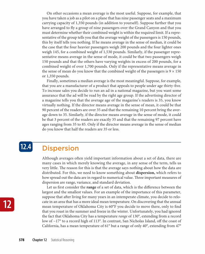
For a fi nal example that illustrates the importance of dispersion, suppose that you decide to put your life savings into a business that designs and manufactures women’s dresses. As corporation president you decide to save money by restricting production to dresses that fi t the average woman. Because the average size in the sense of mean, median, and mode is 12, you decide to make only size 12 dresses. Unfortunately, you later discover that while size 12 is indeed the average, 95 percent of women fall outside this interval, as Figure 12.5 shows.

The problem is that you failed to take into account the standard deviation. If the standard deviation were relatively small, then most of the dress sizes would be

Figure 12.3a Figure 12.3 b

57 59 61 63 65 67 69 71 73

12

Section 12.5 Graphs and Pictograms 583

clustered about the mean (size 12). But in fact the standard deviation is relatively large, so most of the dress sizes fall outside this interval.

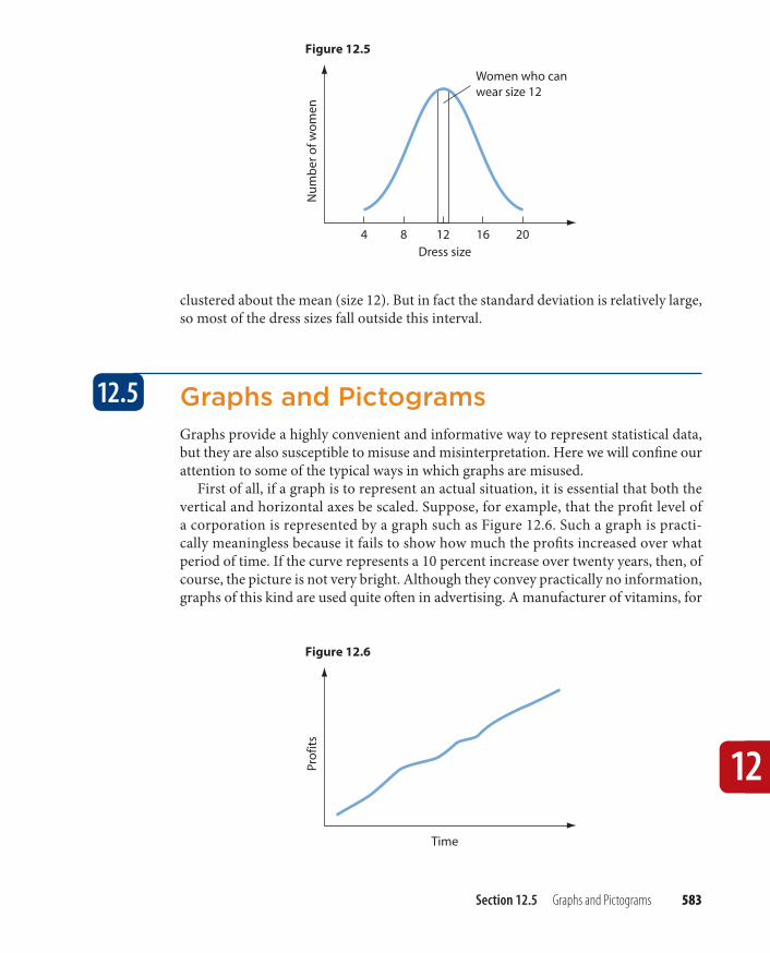
Graphs and PictogramsGraphs provide a highly convenient and informative way to represent statistical data, but they are also susceptible to misuse and misinterpretation. Here we will confi ne our attention to some of the typical ways in which graphs are misused.

First of all, if a graph is to represent an actual situation, it is essential that both the vertical and horizontal axes be scaled. Suppose, for example, that the profi t level of a corporation is represented by a graph such as Figure 12.6. Such a graph is practi-cally meaningless because it fails to show how much the profi ts increased over what period of time. If the curve represents a 10 percent increase over twenty years, then, of course, the picture is not very bright. Although they convey practically no information, graphs of this kind are used quite oft en in advertising. A manufacturer of vitamins, for

12.5

Nu

mb

er o

f wo

men

4 8 12 16Dress size

20

Women who canwear size 12

Figure 12.5

Pro

fits

Time

Figure 12.6

584 Chapter 12 Statistical Reasoning

12

example, might print such a graph on the label of the bottle to suggest that a person’s energy level is supposed to increase dramatically aft er taking the tablets. Such ads fre-quently make an impression because they look scientifi c, and the viewer rarely bothers to check whether the axes are scaled or precisely what the curve is supposed to signify.

A graph that more appropriately represents corporate profi ts is given in Figure 12.7 (the corporation is fi ctitious).

Pro

fits

(mill

ion

s o

f do

llars

)

Quarter

Tangerine Computers, 2010

1 2 3 4

10

9

8

Figure 12.8

Pro

fits

(mill

ion

s o

f do

llars

)

Quarter

Tangerine Computers, 2010

1 2 3 4

15

10

5

Figure 12.7

Inspection of the graph reveals that between January and December profi ts rose from $8 to $10 million, which represents a respectable 25 percent increase. Th is increase can be made to appear even more impressive by chopping off the bottom of the graph and altering the scale on the vertical axis while leaving the horizontal scale as is (Figure 12.8). Again, strictly speaking, the graph accurately represents the facts, but if the viewer fails to notice what has been done to the vertical scale, he or she is liable to derive the impression that the profi ts have increased by something like a hundred percent or more.

12

Section 12.5 Graphs and Pictograms 585

The same strategy can be used with bar graphs. The graphs in Figure 12.9 com-pare sales volume for two consecutive years, but the one on the right conveys the message more dramatically. Of course, if the sales volume has decreased, the corporate directors would probably want to minimize the diff erence, in which case the design on the left is preferable.

Tota

l sal

es (t

ho

usa

nd

s o

f un

its)

TangerineComputers

2009

8

7

6

5

4

3

2

1

2010

Tota

l sal

es (t

ho

usa

nd

s o

f un

its)

TangerineComputers

2009

8

7

6

2010

Figure 12.9

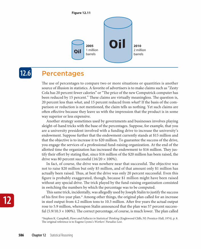
An even greater illusion can be created with the use of pictograms. A pictogram is a diagram that compares two situations through drawings that diff er either in size or in the number of entities depicted. Consider Figure 12.10, which illustrates the increase in production of an oil company between 2005 and 2010.

20051 millionbarrels

20102 millionbarrels

Figure 12.10

Th is pictogram accurately represents the increase because it unequivocally shows that the amount doubled between the years represented. But the eff ect is not especially dramatic. Th e increase in production can be exaggerated by representing the 2010 level with an oil barrel twice as tall (Figure 12.11).

Even though the actual production is stated adjacent to each drawing, this pictogram creates the illusion that production has much more than doubled. While the drawing on the right is exactly twice as high as the one on the left , it is also twice as wide. Th us, it occupies four times as much room on the page. Furthermore, when the viewer’s three-dimensional judgment is called into play, the barrel on the right is perceived as having eight times the volume of the one on the left . Th us, when the third dimension is taken into account, the increase in consumption is exaggerated by 600 percent.

586 Chapter 12 Statistical Reasoning

12

PercentagesTh e use of percentages to compare two or more situations or quantities is another source of illusion in statistics. A favorite of advertisers is to make claims such as “Zesty Cola has 20 percent fewer calories” or “Th e price of the new Computrick computer has been reduced by 15 percent.” Th ese claims are virtually meaningless. Th e question is, 20 percent less than what, and 15 percent reduced from what? If the basis of the com-parison or reduction is not mentioned, the claim tells us nothing. Yet such claims are oft en eff ective because they leave us with the impression that the product is in some way superior or less expensive.

Another strategy sometimes used by governments and businesses involves playing sleight-of-hand tricks with the base of the percentages. Suppose, for example, that you are a university president involved with a funding drive to increase the university’s endowment. Suppose further that the endowment currently stands at $15 million and that the objective is to increase it to $20 million. To guarantee the success of the drive, you engage the services of a professional fund-raising organization. At the end of the allotted time the organization has increased the endowment to $16 million. Th ey jus-tify their eff ort by stating that, since $16 million of the $20 million has been raised, the drive was 80 percent successful (16/20 × 100%).

In fact, of course, the drive was nowhere near that successful. Th e objective was not to raise $20 million but only $5 million, and of that amount only $1 million has actually been raised. Th us, at best the drive was only 20 percent successful. Even this fi gure is probably exaggerated, though, because $1 million might have been raised without any special drive. Th e trick played by the fund-raising organization consisted in switching the numbers by which the percentage was to be computed.

Th is same trick, incidentally, was allegedly used by Joseph Stalin to justify the success of his fi rst fi ve-year plan.* Among other things, the original plan called for an increase in steel output from 4.2 million tons to 10.3 million. Aft er fi ve years the actual output rose to 5.9 million, whereupon Stalin announced that the plan was 57 percent success-ful (5.9/10.3 × 100%). Th e correct percentage, of course, is much lower. Th e plan called

*Stephen K. Campbell, Flaws and Fallacies in Statistical Th inking (Englewood Cliff s, NJ: Prentice-Hall, 1974), p. 8. Th e original reference is to Eugene Lyons’s Workers’ Paradise Lost.

12.6

20051 millionbarrels

20102 millionbarrels

Figure 12.11

12

Section 12.6 Percentages 587

for an increase of 6.1 million tons and the actual increase was only 1.7  million. Th us, at best, the plan was only 28 percent successful.

Similar devices have been used by employers on their unsuspecting employ-ees. When business is bad, an employer may argue that salaries must be reduced by 20  percent. Later, when business improves, salaries will be raised by 20 percent, thus restoring them to their original level. Such an argument, of course, is fallacious. If a person earns $10 per hour and that person’s salary is reduced by 20 percent, the adjusted salary is $8. If that fi gure is later increased by 20 percent, the fi nal salary is $9.60. Th e problem, of course, stems from the fact that a diff erent base is used for the two percentages. Th e fallacy committed by such arguments is a variety of equivocation. Percentages are relative terms, and they mean diff erent things in diff erent contexts.

A diff erent kind of fallacy occurs when a person attempts to add percentages as if they were cardinal numbers. Suppose, for example, that a baker increases the price of a loaf of bread by 50 percent. To justify the increase the baker argues that it was necessitated by rising costs: Th e price of fl our increased by 10 percent, the cost of labor rose 20  percent, utility rates went up 10 percent, and the cost of the lease on the building increased 10 percent. Th is adds up to a 50 percent increase. Again, the argument is fallacious. If everything had increased by 20 percent, this would justify only a 20 percent increase in the price of bread. As it is, the justifi ed increase is less than that. Th e fallacy committed by such arguments would probably be best classifi ed as a case of missing the point (igno-ratio elenchi). Th e arguer has failed to grasp the signifi cance of his own premises.

Statistical variations of the suppressed evidence fallacy are also quite common. One variety consists in drawing a conclusion from a comparison of two diff erent things or situations. For example, people running for political offi ce sometimes cite fi gures indicating that crime in the community has increased by, let us say, 20 percent during the past three or four years. What is needed, they conclude, is an all-out war on crime. But they fail to mention that the population in the community has also increased by 20 percent during the same period. Th e number of crimes per capita, therefore, has not changed. Another example of the same fallacy is provided by the ridiculous argument that 90 percent more traffi c accidents occur in clear weather than in foggy weather and that therefore it is 90 percent more dangerous to drive in clear than in foggy weather. Th e arguer ignores the fact that the vast percentage of vehicle miles are driven in clear weather, which accounts for the greater number of accidents.

A similar misuse of percentages is committed by businesses and corporations that, for whatever reason, want to make it appear that they have earned less profit than they actually have. Th e technique consists of expressing profi t as a percentage of sales volume instead of as a percentage of investment. For example, during a certain year a corporation might have a total sales volume of $100 million, a total investment of $10 million, and a profi t of $5 million. If profi ts are expressed as a percentage of invest-ment, they amount to a heft y 50 percent; but as a percentage of sales they are only 5 percent. To appreciate the fallacy in this procedure, consider the case of the jewelry merchant who buys one piece of jewelry each morning for $9 and sells it in the evening for $10. At the end of the year the total sales volume is $3,650, the total investment $9, and the total profi t $365. Profi ts as a percentage of sales amount to only 10 percent, but as a percentage of investment they exceed 4,000 percent.

12

588 Chapter 12 Statistical Reasoning

Exercise 12

I. Criticize the following arguments in light of the material presented in this section: ★1. To test the algae content in a lake, a biologist took a sample of the water at one

end. Th e algae in the sample registered 5 micrograms per liter. Th erefore, the algae in the lake at that time registered 5 micrograms per liter.

2. To estimate public support for a new municipality-funded convention center, researchers surveyed 100 homeowners in one of the city’s fashionable neigh-borhoods. They found that 89 percent of those sampled were enthusiastic about the project. Th erefore, we may conclude that 89 percent of the city’s residents favor the convention center.

3. A quality-control inspector for a food-processing fi rm needed assurance that the cans of fruit in a production run were fi lled to capacity. He opened every tenth box in the warehouse and removed the can in the left front corner of each box. He found that all of these cans were fi lled to capacity. Th erefore, it is probable that all of the cans in the production run were fi lled to capacity.

★4. When a random sample of 600 voters was taken on the eve of the presidential election, it was found that 51 percent of those sampled intended to vote for the Democrat and 49 percent for the Republican. Th erefore, the Democrat will probably win.

5. To determine the public’s attitude toward TV soap operas, 1,000 people were contacted by telephone between 8:00 a.m. and 5:00 p.m. on weekdays. Th e numbers were selected randomly from the phone directories of cities across the nation. Th e researchers reported that 43 percent of the respondents said that they were avid viewers. From this we may conclude that 43 percent of the public watches TV soap operas.

6. To predict the results of a U.S. Senate race in New York State, two polls were taken. One was based on a random sample of 750 voters, the other on a ran-dom sample of 1,500 voters. Since the second sample was twice as large as the fi rst, the results of the second poll were twice as accurate as the fi rst.

★7. In a survey conducted by the manufacturers of Ultrasheen toothpaste, 65 per-cent of the dentists randomly sampled preferred that brand over all others. Clearly Ultrasheen is the brand preferred by most dentists.

8. To determine the percentage of adult Americans who have never read the U.S. Constitution, surveyors put this question to a random sample of 1,500 adults. Only 13 percent gave negative answers. Th erefore, since the sampling error for such a sample is 3 percent, we may conclude that no more than 16 percent of American adults have not read the Constitution.

9. To determine the percentage of patients who follow the advice of their per-sonal physician, researchers asked 200 randomly chosen physicians to put the question to their patients. Of the 4,000 patients surveyed, 98 percent replied

Section 12.6 Percentages 589

12

that they did indeed follow their doctor’s advice. We may therefore conclude that at least 95 percent of the patients across the nation follow the advice of their personal physician.

★10. Janet Ryan can aff ord to pay no more than $15 for a birthday gift for her eight-year-old daughter. Since the average price of a toy at General Toy Company is $15, Janet can expect to fi nd an excellent selection of toys within her price range at that store.

11. Anthony Valardi, who owns a fi sh market, pays $2 per pound to fi shermen for silver salmon. A certain fi sherman certifi es that the average size of the salmon in his catch of the day is 10 pounds, and that the catch numbers 100 salmon. Mr. Valardi is therefore justifi ed in paying the fi sherman $2,000 for the whole catch.

12. Pamela intends to go shopping for a new pair of shoes. She wears size 8. Since the average size of the shoes carried by the Bon Marche is size 8, Pamela can expect to fi nd an excellent selection of shoes in her size at that store.

★13. Tim Cassidy, who works for a construction company, is told to load a pile of rocks onto a truck. Th e rocks are randomly sized, and the average piece weighs 50 pounds. Th us, Tim should have no trouble loading the rocks by hand.

14. Th e average IQ (in the sense of mean, median, and mode) of the students in Dr. Jacob’s symbolic logic class is 120. Th us, none of the students should have any trouble mastering the subject matter.

15. An insecticide manufacturer prints the following graph on the side of its spray cans:

Nu

mb

er o

f bu

gs

kille

d

Time

After one application

Obviously, the insecticide is highly eff ective at killing bugs, and it keeps work-ing for a long time.

★16. A corporation’s sales for two consecutive years are represented in a bar graph. Since the bar for the later year is twice as high as the one for the previous year, it follows that sales for the later year were double those for the previous year.

17. Forced to make cutbacks, the president of a manufacturing fi rm reduced cer-tain costs as follows: advertising by 4 percent, transportation by 5 percent,

12

590 Chapter 12 Statistical Reasoning

materials by 2 percent, and employee benefi ts by 3 percent. Th e president thus succeeded in reducing total costs by 14 percent.

18. During a certain year, a grocery store chain had total sales of $100 million and profi ts of $10 million. Th e profi ts thus amounted to a modest 10 percent for that year.

★19. Th ere were 20 percent more traffi c accidents in 2005 than there were in 1980. Th erefore, it was 20 percent more dangerous to drive a car in 2005 than it was in 1980.

20. An effi ciency expert was hired to increase the productivity of a manufactur-ing fi rm and was given three months to accomplish the task. At the end of the period the productivity had increased from 1,500 units per week to 1,700. Since the goal was 2,000 units per week, the eff ort of the effi ciency expert was 85 percent successful (1,700/2,000).

II. Compute the answers to the following questions. ★1. What fi gures should be written in the left -hand column of Table 12.1 to pro-

duce a similar table based on a confi dence level of 99 percent? For a confi dence level of 99 percent, the margin of error is approximately equal to 1.29/√n.

2. Given the following group of people together with their weights, what is the average weight in the sense of mean, median, and mode?

Number of people Weight

2 150

4 160

3 170

1 180

1 190

1 200

1 220

2 230

3. Given the following group of people together with their salaries, what is the average salary in the sense of mean, median, and mode?

Number of people Salary

1 $95,000

2 85,000

1 70,000

3 40,000

1 30,000

2 20,000

5 15,000

Section 12.6 Percentages 591

12

★4. A day-care center cares for ten children. Th eir ages are 1, 1, 2, 2, 2, 3, 3, 4, 6, 6. Construct a histogram that represents the distribution of ages. What is the mean age? What is the variance and standard deviation of these ages?

5. A small company has fi ve employees who missed work during a certain month. Th e number of days missed were 1, 1, 2, 4, 7. What is the mean number of days missed? What is the variance and standard deviation of this set of data?

6. An instructor gave a ten-question multiple-choice quiz to twelve students. Th e scores were 10, 10, 9, 9, 8, 8, 8, 7, 7, 7, 7, 6. What is the mean score? What is the variance and standard deviation of these scores?

III. Answer “true” or “false” to the following statements: ★1. If a sample is very large, it need not be randomly selected. 2. If a population is randomly arranged, a sample obtained by selecting every

tenth member would be a random sample. 3. If a sample is randomly selected, the larger the sample is, the more closely it

replicates the population. ★4. To ensure the same precision, a population of 1 million would require a much

larger random sample than would a population of 100,000. 5. In general, if sample A is twice as large as sample B, then the sampling error

for A is one-half that for B. 6. When a sample consists of human beings, the purpose for which the sample is

taken can aff ect the outcome. ★7. Th e personal interaction between a surveyor and a respondent can aff ect the

outcome of a survey. 8. The mean value of a set of data is the value that occurs with the greatest

frequency. 9. Th e median value of a set of data is the middle point when the data are arr-

anged in ascending order. ★10. Th e modal value of a set of data is the arithmetical average. 11. If one needed to know whether a sizable portion of a group were above or

below a certain level, the most useful sense of average would be mode. 12. Data refl ecting the results of a random sample conform fairly closely to the

normal probability distribution. ★13. If a set of data conform to the normal probability distribution, then the mean,

median, and mode have the same value. 14. Range, variance, and standard deviation are measurements of dispersion. 15. Statements about averages oft en present an incomplete picture, lacking infor-

mation about the dispersion. ★16. Data refl ecting the size of full-grown horses would exhibit greater dispersion

than would data refl ecting the size of full-grown dogs. 17. Th e visual impression made by graphs can be exaggerated by changing one of

the scales while leaving the other unchanged.

12

592 Chapter 12 Statistical Reasoning

18. Data reflecting a 100 percent increase in housing construction could be accurately represented by a pictogram of two houses, one twice as high as the other.

★19. If a certain quantity is increased by 10 percent and later decreased by 10  percent, the quantity is restored to what it was originally.

20. Expressing profi ts as a percentage of sales volume presents an honest picture of the earnings of a corporation.

Summary

Statistical Reasoning

• Includes any kind of argumentation based on statistical measurement.

• Such arguments can be misleading for several reasons: ■ Biased samples:

▶ Not randomly selected

▶ Too small (Note sampling error.)

▶ Psychological factors ■ Diff erent meaning for “average”:

▶ Mean (the numerical average)

▶ Median (the mid-point)

▶ Mode (the value that occurs with the greatest frequency) ■ Failure to take dispersion into account:

▶ Range (diff erence between largest and smallest values)

▶ Variance (how much every data point varies from the mean)

▶ Standard deviation (square root of the variance) ■ Illusory graphs

▶ Failure to scale the axes

▶ Chopping off the bottom of the graph

▶ Altering the scale of the axes ■ Illusory pictograms

▶ Illusions related to spatial dimensions ■ Improper percentages:

▶ Failure to state the base of the percentage

▶ Slight-of-hand tricks with the base

▶ Numerical errors