A Computational Clonal Analysis of the Developing Mouse ...
16
A Computational Clonal Analysis of the Developing Mouse Limb Bud Luciano Marcon 1 *, Carlos G. Arque ´s 2 , Miguel S. Torres 2 , James Sharpe 1,3 * 1 EMBL-CRG Systems Biology Research Unit, Center for Genomic Regulation (CRG), Universitat Pompeu Fabra, Barcelona, Spain, 2 Departamento de Biologı ´a del Desarrollo Cardiovascular, Centro Nacional de Investigaciones Cardiovasculares (CNIC), Instituto de Salud Carlos III, Madrid, Spain, 3 ICREA Professor, Centre for Genomic Regulation (CRG), Universitat Pompeu Fabra, Barcelona, Spain Abstract A comprehensive spatio-temporal description of the tissue movements underlying organogenesis would be an extremely useful resource to developmental biology. Clonal analysis and fate mappings are popular experiments to study tissue movement during morphogenesis. Such experiments allow cell populations to be labeled at an early stage of development and to follow their spatial evolution over time. However, disentangling the cumulative effects of the multiple events responsible for the expansion of the labeled cell population is not always straightforward. To overcome this problem, we develop a novel computational method that combines accurate quantification of 2D limb bud morphologies and growth modeling to analyze mouse clonal data of early limb development. Firstly, we explore various tissue movements that match experimental limb bud shape changes. Secondly, by comparing computational clones with newly generated mouse clonal data we are able to choose and characterize the tissue movement map that better matches experimental data. Our computational analysis produces for the first time a two dimensional model of limb growth based on experimental data that can be used to better characterize limb tissue movement in space and time. The model shows that the distribution and shapes of clones can be described as a combination of anisotropic growth with isotropic cell mixing, without the need for lineage compartmentalization along the AP and PD axis. Lastly, we show that this comprehensive description can be used to reassess spatio-temporal gene regulations taking tissue movement into account and to investigate PD patterning hypothesis. Citation: Marcon L, Arque ´s CG, Torres MS, Sharpe J (2011) A Computational Clonal Analysis of the Developing Mouse Limb Bud. PLoS Comput Biol 7(2): e1001071. doi:10.1371/journal.pcbi.1001071 Editor: Stanislav Shvartsman, Princeton University, United States of America Received August 11, 2010; Accepted December 29, 2010; Published February 10, 2011 Copyright: ß 2011 Marcon et al. This is an open-access article distributed under the terms of the Creative Commons Attribution License, which permits unrestricted use, distribution, and reproduction in any medium, provided the original author and source are credited. Funding: The work was funded by the MADRICEL grant from the Madrid Regional Government (S-SAL-0190-2006). The funders had no role in study design, data collection and analysis, decision to publish, or preparation of the manuscript. Competing Interests: The authors have declared that no competing interests exist. * E-mail: [email protected] (LM); [email protected] (JS) Introduction The cellular processes by which a field of cells develops into a spatially-organized tissue have traditionally been split into two distinct questions: pattern formation and morphogenesis. The first focuses on the regulatory mechanisms underlying spatial and temporal cell fate specification. The second focuses on the cellular behaviors that physically drive growth and shaping of multicellular structures. While these two processes can indeed be considered to be conceptually separated, in practice they usually occur simultaneously and are believed to be tightly coordinated. The vertebrate limb is an excellent model system to study how these two processes work in combination [1]. In mouse, limb development starts around 9 days post fertilization with the protrusion of a mass of undifferentiated mesenchymal cells from the lateral plate mesoderm of the embryo. This structure, known as the limb bud, is able to grow and organize itself in less than 3 days to determine most of the structures found in the adult limb (tendons, skeleton, dermis etc.). Growth and patterning occur along three major axes: the proximal-distal axis (PD) that goes from the body to the finger tip; the anterior-posterior axis (AP) going from the thumb to the little finger and the dorsal-ventral axis (DV), going from the palm to the dorsal part of the limb. Important signaling centers of the limb, like the apical ectodermal ridge (AER) and the zone of polarizing activity (ZPA), are known to regulate both growth and patterning [2–4] and their activities are known to be highly coupled [5]. Moreover there is increasing evidence that tissue growth could play an important role for patterning [6]. Therefore a crucial step to better understand both limb morphogenesis and patterning is to accurately map tissue movements over space and time. Several studies in chick [7–9] have produced fate maps which provide an important overview of the tissue movements in the mesenchyme and in the AER. In mouse, where in utero labeling is required, a first study was made in [10] by carbon particles injection and only more recently a first clonal analysis was performed by using a tamoxifen-inducible Cre reporter line to obtain cell labeling in the embryo [11]. However, the goal of these studies was not to build quantitatively-accurate maps of tissue movements, but rather to address specific questions about (a) the timing and mechanisms of regional fate determination, and (b) the possible presence of lineage-restriction compartments. It has been possible to draw clear conclusions regarding the second question: a clear compartment boundary restricting cells along the DV axis was found in [11], while no evidence for compartments along the other two axes was found (PD and AP). Indeed, both in chick and mouse a high degree of overlap was found between clones of the three PD regions corresponding to the stypolod, zeugopod and PLoS Computational Biology | www.ploscompbiol.org 1 February 2011 | Volume 7 | Issue 2 | e1001071
Transcript of A Computational Clonal Analysis of the Developing Mouse ...

A Computational Clonal Analysis of the DevelopingMouse Limb BudLuciano Marcon1*, Carlos G. Arques2, Miguel S. Torres2, James Sharpe1,3*
1 EMBL-CRG Systems Biology Research Unit, Center for Genomic Regulation (CRG), Universitat Pompeu Fabra, Barcelona, Spain, 2 Departamento de Biologıa del Desarrollo
Cardiovascular, Centro Nacional de Investigaciones Cardiovasculares (CNIC), Instituto de Salud Carlos III, Madrid, Spain, 3 ICREA Professor, Centre for Genomic Regulation
(CRG), Universitat Pompeu Fabra, Barcelona, Spain
Abstract
A comprehensive spatio-temporal description of the tissue movements underlying organogenesis would be an extremelyuseful resource to developmental biology. Clonal analysis and fate mappings are popular experiments to study tissuemovement during morphogenesis. Such experiments allow cell populations to be labeled at an early stage of developmentand to follow their spatial evolution over time. However, disentangling the cumulative effects of the multiple eventsresponsible for the expansion of the labeled cell population is not always straightforward. To overcome this problem, wedevelop a novel computational method that combines accurate quantification of 2D limb bud morphologies and growthmodeling to analyze mouse clonal data of early limb development. Firstly, we explore various tissue movements that matchexperimental limb bud shape changes. Secondly, by comparing computational clones with newly generated mouse clonaldata we are able to choose and characterize the tissue movement map that better matches experimental data. Ourcomputational analysis produces for the first time a two dimensional model of limb growth based on experimental datathat can be used to better characterize limb tissue movement in space and time. The model shows that the distribution andshapes of clones can be described as a combination of anisotropic growth with isotropic cell mixing, without the need forlineage compartmentalization along the AP and PD axis. Lastly, we show that this comprehensive description can be usedto reassess spatio-temporal gene regulations taking tissue movement into account and to investigate PD patterninghypothesis.
Citation: Marcon L, Arques CG, Torres MS, Sharpe J (2011) A Computational Clonal Analysis of the Developing Mouse Limb Bud. PLoS Comput Biol 7(2):e1001071. doi:10.1371/journal.pcbi.1001071
Editor: Stanislav Shvartsman, Princeton University, United States of America
Received August 11, 2010; Accepted December 29, 2010; Published February 10, 2011
Copyright: � 2011 Marcon et al. This is an open-access article distributed under the terms of the Creative Commons Attribution License, which permitsunrestricted use, distribution, and reproduction in any medium, provided the original author and source are credited.
Funding: The work was funded by the MADRICEL grant from the Madrid Regional Government (S-SAL-0190-2006). The funders had no role in study design, datacollection and analysis, decision to publish, or preparation of the manuscript.
Competing Interests: The authors have declared that no competing interests exist.
* E-mail: [email protected] (LM); [email protected] (JS)
Introduction
The cellular processes by which a field of cells develops into a
spatially-organized tissue have traditionally been split into two
distinct questions: pattern formation and morphogenesis. The first
focuses on the regulatory mechanisms underlying spatial and
temporal cell fate specification. The second focuses on the cellular
behaviors that physically drive growth and shaping of multicellular
structures. While these two processes can indeed be considered to
be conceptually separated, in practice they usually occur
simultaneously and are believed to be tightly coordinated. The
vertebrate limb is an excellent model system to study how these
two processes work in combination [1]. In mouse, limb
development starts around 9 days post fertilization with the
protrusion of a mass of undifferentiated mesenchymal cells from
the lateral plate mesoderm of the embryo. This structure, known
as the limb bud, is able to grow and organize itself in less than 3
days to determine most of the structures found in the adult limb
(tendons, skeleton, dermis etc.). Growth and patterning occur
along three major axes: the proximal-distal axis (PD) that goes
from the body to the finger tip; the anterior-posterior axis (AP)
going from the thumb to the little finger and the dorsal-ventral axis
(DV), going from the palm to the dorsal part of the limb.
Important signaling centers of the limb, like the apical ectodermal
ridge (AER) and the zone of polarizing activity (ZPA), are known
to regulate both growth and patterning [2–4] and their activities
are known to be highly coupled [5]. Moreover there is increasing
evidence that tissue growth could play an important role for
patterning [6]. Therefore a crucial step to better understand both
limb morphogenesis and patterning is to accurately map tissue
movements over space and time.
Several studies in chick [7–9] have produced fate maps which
provide an important overview of the tissue movements in the
mesenchyme and in the AER. In mouse, where in utero labeling is
required, a first study was made in [10] by carbon particles
injection and only more recently a first clonal analysis was
performed by using a tamoxifen-inducible Cre reporter line to
obtain cell labeling in the embryo [11]. However, the goal of these
studies was not to build quantitatively-accurate maps of tissue
movements, but rather to address specific questions about (a) the
timing and mechanisms of regional fate determination, and (b) the
possible presence of lineage-restriction compartments. It has been
possible to draw clear conclusions regarding the second question: a
clear compartment boundary restricting cells along the DV axis
was found in [11], while no evidence for compartments along the
other two axes was found (PD and AP). Indeed, both in chick and
mouse a high degree of overlap was found between clones of the
three PD regions corresponding to the stypolod, zeugopod and
PLoS Computational Biology | www.ploscompbiol.org 1 February 2011 | Volume 7 | Issue 2 | e1001071

autopod. However, regarding the first question, experimental
results have led to conflicting interpretations. For example, the
relationship between PD patterning and the underlying tissue
movement remains unclear. On one hand, limb tissue movement
data has been used to support the idea that the three PD segments
are specified at early stages of limb development [12] and
subsequently only expand because of growth. On the other hand,
comparisons between fate maps and the expression of distal
markers like Hox genes [9,13] have been used to support the idea
that the PD patterning relies on complex spatio-temporal gene
regulation coordinated with growth [14,15].
Discrepancies between different interpretations of tissue move-
ment data are due to a few specific limitations of previous studies
which we aim to address through the modeling framework
presented here. Firstly, quantitative details matter. Although
alternative hypotheses may be qualitatively different from each
other (such as the Progress Zone Model (PZM) [16] versus the
Early Specification Model (ESM) [12]), the empirical evidence that
could distinguish them will often depend on quantitative details of
timing. Previous projects have revealed the overall pattern of
movements, but have not mapped out the quantitative details.
Secondly, all real data sets are sparse – they provide observations
about a discrete collection of positions in space and time. It is non-
trivial to extrapolate from these observations to a comprehensive
prediction of how any piece of tissue will move at any point in
time. Thirdly, many projects have employed a large time interval
between labeling the cells and assessing the distribution of
descendants. The shapes of the final labeled regions are therefore
the result of an accumulated history of different tissue movements
over time. Again, deconstructing the full sequence of local
movements which lead to the final result is non-trivial. In
particular, a recent study [17] showed that the tissue movements
that drive limb morphogenesis are more complex than previously
thought and depend on anisotropic forces. This and other studies
[18,19] also highlighted that limb mesenchymal cells have a
complex shape and are capable of a wide range of cellular
behaviors including oriented cell division and cell migration.
As an important step beyond the general overview given by
previous fate maps, a formal numerical description of limb tissue
movements over time would be of immense help to analyze the
complex morphogenesis of the limb. Such a description could be
defined by the velocity vectors defining the displacement of each
tissue point in a fixed coordinate system. Ideally, the collection of
these vectors, known as velocity vector field, would be directly
measured by tracking tissue points during growth by time-lapse
imaging. However, despite recent advances in live imaging of the
mammalian limb bud [20,21], it is a challenging technique and a
complete description of tissue movements is still not available. In
plants, clonal analysis has been explored as an alternative to live
imaging for studying the growth of 2D leaves and petals. Local
growth tensors were derived directly from shapes of clones and
these data were combined into a computational model to recreate
a full map of the global tissue movements (the velocity vector field)
over time [22]. Unfortunately, in the mouse limb most of the
available fate maps and clonal analyses have been performed with
a long time-interval between labeling and analysis. This is ideal for
the more common purpose of fate-mapping, as it reveals the final
positions and tissue types of cells which were labeled during their
early patterning phase. However such long-term clone shapes are
not suitable for directly inferring local growth tensors – instead
labeled populations should have undergone only enough growth to
reveal local anisotropies, i.e. a short time-interval between labeling
and analysis [23]. Another complication compared to the 2D plant
case is the extensive mixing of mesenchymal cells that leads to a
strong dispersal of the cells over space. A velocity vector field alone
would therefore be insufficient to fully describe cell movements.
Due to this lack of quantitative data on tissue movements, most
of the existing 2D mathematical models of limb growth have been
used as theoretical tools to explore possible cellular hypothesis
explaining limb outgrowth [24,25]. These studies relied on the
existing literature to suggest the underlying mechanics of limb
growth, and consequently predicted tissue movement maps
consistent with the proliferation gradient hypothesis [26], in
which tissue expansion is concentrated at the distal tip. However,
a recent simulation which performed a more rigorous compar-
ison of this hypothesis against quantitative data on proliferation
rates, has demonstrated the implausibility of this concept [17].
Since it is now clear that the cellular mechanics underlying
outgrowth are complex and not well understood [19,27], we
therefore wished to create a model of tissue movements which is
based not on a mechanistic hypothesis, but which instead acts as
a numerically-descriptive framework within which to integrate
information from real clonal experiments. In particular we have
developed a methodology which is not restricted to short-term
clonal data, and which can interpret the available long-term
clonal and predict cell movements across the full spatio-temporal
extent of mouse limb bud development. The model is able to use
2 sources of data as empirical constraints to define a biologically-
accurate tissue movement map: (i) a temporal sequence of
experimental limb bud morphologies – a numerical shape
description for every hour of development over a 72 hour
period, and (ii) a collection of clonal data generated by a
tamoxifen-inducible Cre transgenic mouse line.
The paper is organized as follows. In the first two sections of
the results we introduce the new computational approach that
was developed to explore different limb tissue movement maps
matching experimental change in limb morphology. In the
subsequent two sections we present a mouse clonal analysis of
early limb development (from 9 to 12 days pf.) and we show how
the tissue movement map that better matched the distribution
and shapes of clones was selected. In the following section, the
tissue movement map is modified to match the experimental
degree of cell mixing observed in the experimental clones. In the
Author Summary
A comprehensive mathematical description of the growthof an organ can be given by the velocity vectors definingthe displacement of each tissue point in a fixed coordinatesystem plus a description of the degree of mixing betweenthe cells. As an alternative to live imaging, a way toestimate the collection of such velocity vectors, known asvelocity vector field, is to use cell-labeling experiments.However, this approach can be applied only when thelabeled populations have been grown for small periods oftime and the tensors of the velocity vector field can beestimated directly from the shape of the labeled popula-tion. Unfortunately, most of the available cell-labelingexperiments of developmental systems have been gener-ated considering a long clone expansion time that is moresuitable for lineaging studies than for estimating velocityvector fields. In this study we present a new computationalmethod that allows us to estimate the velocity vector fieldof limb tissue movement by using clonal data with longharvesting time and a sequence of experimental limbmorphologies. The method results in the first realistic 2Dmodel of limb outgrowth and establishes a powerfulframework for numerical simulations of limb development.
A Computational Clonal Analysis of the Limb Bud
PLoS Computational Biology | www.ploscompbiol.org 2 February 2011 | Volume 7 | Issue 2 | e1001071

last section of the results we characterize the tissue movement
map and relate it to traditional PD patterning hypothesis. Finally
in the Discussion section we summarize the study and present the
future applications of the model.
Results
We present here a new computational method that estimates the
velocity vector field of limb tissue movement by using 2
experimental constraints: a sequence of experimental limb mor-
phologies, and long-term clonal data. The main idea underlying the
method is to generate a set of hypothetical velocity vector fields that
are consistent with the first constraint (the experimental morpho-
logical changes), and then to select the one responsible for real limb
outgrowth by comparing simulated fate maps with the second
constraint (the experimental clonal data). In this respect our
approach is analogous to a ‘‘reverse-engineering’ method, as the
data cannot lead to a direct calculation of tissue movements but can
only constrain the possible forward simulations. The resulting
velocity vector field was then used to derive the tensors of the
velocity gradient which describe the local behaviors of the tissue
movement. As an application of the model, a reverse version of the
tissue movement map was generated to provide a relative estimate
of the degree of mixing between the progenitors of three PD
segments. Finally, by mapping a time course of Hoxd13 gene
expression into the model, we were able reveal the contribution of
tissue movement to the expansion of the Hoxd13 domain.
From 2D experimental morphologies to velocity vectorfields
The shape of the limb bud at any point in time can be defined by
a spline curve, but clear morphological features along this line are
absent – the limb displays a smooth rounded shape. This lack of
landmarks means that even a very precise knowledge of the shapes
over time is insufficient to define the underlying tissue movements.
This is true both for the internal tissue and also the limb boundary
itself, as a particular point of tissue (or landmark) could slide along
the boundary spline without altering the shape. Figure 1 illustrates
the nature of the problem: a well-defined shape change is given
(panel A), but numerous different tissue movement maps are all
equally compatible with this observation, each of which has
different combinations of local tissue speed and directionality (B–
E). Despite these degrees-of-freedom, the temporal sequence of
boundary shapes does nevertheless act as an important constraint
on the full range of growth possibilities. To capture an accurate
numerical description of these shape changes we therefore took
advantage of a morphometric analysis performed in [28]. In that
work, 600 limb buds of different ages were photographed in a
standard orientation, cubic splines were fitted to the boundaries,
average shapes were calculated for key timepoints, and shape
interpolation was performed to calculate the intermediate shapes
[28]. The result is an hour-by-hour sequence of 72 shapes which
represents a standard trajectory of limb bud morphology over
developmental time (from approximately E9 to E12) – see Figure
S1. Each shape corresponds to a morphometric stage that is named
as mEdd:hh, where dd is the morphometric embryonic day and hh is
the morphometric embryonic hour. It is important to note that the
morphometric stage notation is different from the standard
embryonic day notation, for example the standard notation E10.5
translates into the morphometric stage mE10:12.
For this study we had to develop software that would allow the
exploration of a set of possible velocity vector fields that can each
reproduce the same observed boundary changes. In particular,
different tissue movement maps are equivalent to considering the
2D limb shape as a rubber sheet or mesh, with different distributions
of elastic deformation (e.g.. the various mesh deformations shown in
Figure 1B–E). To cover the whole temporal sequence of
development, a single complete map would include a sequence of
slightly changing hour-by-hour deformations across all 72 shapes.
We thus spatially discretized each of the limb bud shapes using an
unstructured triangular grid. An example of the type of grid
generated is given in Figure 2C. We then sought a convenient
approach to parameterize the variety of possible mesh deformations
across time, and devised a two-step method – the first step dealing
with boundary, and the second with the internal tissue movements.
For the first step, in effect we must define a series of landmarks
which explicitly map points in each boundary shape to their
Figure 1. Different ways to make the same shape. (A) A simplesemi circle (first column) grows into a defined shape (second column).The two shapes are aligned at their left boundary (third column). (B) Avelocity vector field pointing in the distal direction with a vectormagnitude distribution that leads to a uniform expansion. (C–E) Avariety of velocity vector fields which can all create the same boundaryshape change. The first magnitude distribution (C) defines uniformexpansion, the second (D) defines a greater distal expansion and thethird (E) a greater proximal expansion.doi:10.1371/journal.pcbi.1001071.g001
A Computational Clonal Analysis of the Limb Bud
PLoS Computational Biology | www.ploscompbiol.org 3 February 2011 | Volume 7 | Issue 2 | e1001071

A Computational Clonal Analysis of the Limb Bud
PLoS Computational Biology | www.ploscompbiol.org 4 February 2011 | Volume 7 | Issue 2 | e1001071
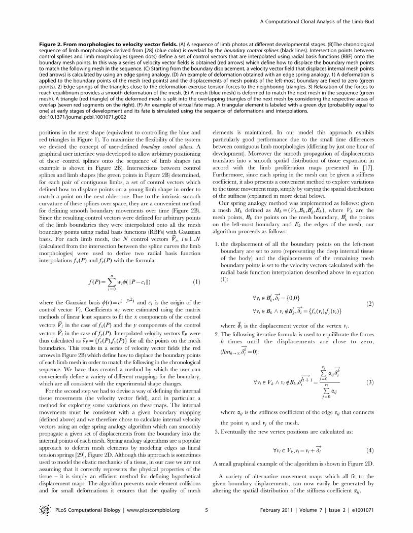
positions in the next shape (equivalent to controlling the blue and
red triangles in Figure 1). To maximize the flexibility of the system
we devised the concept of user-defined boundary control splines. A
graphical user interface was developed to allow arbitrary positioning
of these control splines onto the sequence of limb shapes (an
example is shown in Figure 2B). Intersections between control
splines and limb shapes (the green points in Figure 2B) determined,
for each pair of contiguous limbs, a set of control vectors which
defined how to displace points on a young limb shape in order to
match a point on the next older one. Due to the intrinsic smooth
curvature of these splines over space, they are a convenient method
for defining smooth boundary movements over time (Figure 2B).
Since the resulting control vectors were defined for arbitrary points
of the limb boundaries they were interpolated onto all the mesh
boundary points using radial basis functions (RBFs) with Gaussian
basis. For each limb mesh, the N control vectors ~VVi, i [ 1::N(calculated from the intersection between the spline curves the limb
morphologies) were used to derive two radial basis function
interpolations fx(P) and fy(P) with the formula:
f (P)~Xn
i~0
wiw(EP{ciE) ð1Þ
where the Gaussian basis w(r)~e({br2) and ci is the origin of the
control vector Vi. Coefficients wi were estimated using the matrix
methods of linear least squares to fit the x components of the control
vectors ~VVi in the case of fx(P) and the y components of the control
vectors ~VVi in the case of fy(P). Interpolated velocity vectors~vvP were
thus calculated as~vvP~ffx(P),fy(P)g for all the points on the mesh
boundaries. This results in a series of velocity vector fields (the red
arrows in Figure 2B) which define how to displace the boundary points
of each limb mesh in order to match the following in the chronological
sequence. We have thus created a method by which the user can
conveniently define a variety of different mappings for the boundary,
which are all consistent with the experimental shape changes.
For the second step we had to devise a way of defining the internal
tissue movements (the velocity vector field), and in particular a
method for exploring some variations on these maps. The internal
movements must be consistent with a given boundary mapping
(defined above) and we therefore chose to calculate internal velocity
vectors using an edge spring analogy algorithm which can smoothly
propagate a given set of displacements from the boundary into the
internal points of each mesh. Spring analogy algorithms are a popular
approach to deform mesh elements by modeling edges as lineal
tension springs [29], Figure 2D. Although this approach is sometimes
used to model the elastic mechanics of a tissue, in our case we are not
assuming that it correctly represents the physical properties of the
tissue – it is simply an efficient method for defining hypothetical
displacement maps. The algorithm prevents node element collisions
and for small deformations it ensures that the quality of mesh
elements is maintained. In our model this approach exhibits
particularly good performance due to the small time differences
between contiguous limb morphologies (differing by just one hour of
development). Moreover the smooth propagation of displacements
translates into a smooth spatial distribution of tissue expansion in
accord with the limb proliferation maps presented in [17].
Furthermore, since each spring in the mesh can be given a stiffness
coefficient, it also presents a convenient method to explore variations
to the tissue movement map, simply by varying the spatial distribution
of the stiffness (explained in more detail below).
Our spring analogy method was implemented as follows: given
a mesh Mk defined as Mk~(Vk,Bk,Blk,Ek), where Vk are the
mesh points, Bk the points on the mesh boundary, Blk the points
on the left-most boundary and Ek the edges of the mesh, our
algorithm proceeds as follows:
1. the displacement of all the boundary points on the left-most
boundary are set to zero (representing the deep internal tissue
of the body) and the displacements of the remaining mesh
boundary points is set to the velocity vectors calculated with the
radial basis function interpolation described above in equation
(1):
Vvi [ Blk,di
!~f0,0g
Vvi [ Bk ^ vi [=Blk,di
!~ffx(vi),fy(vi)g
ð2Þ
where ~ddi is the displacement vector of the vertex vi:
2. The following iterative formula is used to equilibrate the forces
h times until the displacements are close to zero,
(limh??dhi
!~0):
Vvi [ Vk ^ vi [=Bk,dhz�!
1i ~
Pvi
j~0
aij dhi
!
Pvi
j~0
aij
ð3Þ
where aij is the stiffness coefficient of the edge eij that connects
the point vi and vj of the mesh.
3. Eventually the new vertex positions are calculated as:
Vvi [ Vk,vi~vizdi
! ð4Þ
A small graphical example of the algorithm is shown in Figure 2D.
A variety of alternative movement maps which all fit to the
given boundary displacements, can now easily be generated by
altering the spatial distribution of the stiffness coefficient aij .
Figure 2. From morphologies to velocity vector fields. (A) A sequence of limb photos at different developmental stages. (B)The chronologicalsequence of limb morphologies derived from [28] (blue color) is overlaid by the boundary control splines (black lines). Intersection points betweencontrol splines and limb morphologies (green dots) define a set of control vectors that are interpolated using radial basis functions (RBF) onto theboundary mesh points. In this way a series of velocity vector fields is obtained (red arrows) which define how to displace the boundary mesh pointsto match the following mesh in the sequence. (C) Starting from the boundary displacement, a velocity vector field that displaces internal mesh points(red arrows) is calculated by using an edge spring analogy. (D) An example of deformation obtained with an edge spring analogy. 1) A deformation isapplied to the boundary points of the mesh (red points) and the displacements of mesh points of the left-most boundary are fixed to zero (greenpoints). 2) Edge springs of the triangles close to the deformation exercise tension forces to the neighboring triangles. 3) Relaxation of the forces toreach equilibrium provides a smooth deformation of the mesh. (E) A mesh (blue mesh) is deformed to match the next mesh in the sequence (greenmesh). A triangle (red triangle) of the deformed mesh is split into the overlapping triangles of the next mesh by considering the respective areas ofoverlap (seven red segments on the right). (F) An example of virtual fate map. A triangular element is labeled with a green dye (probability equal toone) at early stages of development and its fate is simulated using the sequence of deformations and interpolations.doi:10.1371/journal.pcbi.1001071.g002
A Computational Clonal Analysis of the Limb Bud
PLoS Computational Biology | www.ploscompbiol.org 5 February 2011 | Volume 7 | Issue 2 | e1001071

In conclusion, we can define a velocity vector field for each
mesh in the chronological sequence (the red arrows in Figure 2C)
representing a hypothetical tissue movement map connecting each
pair of contiguous morphologies in the sequence, see Video S1.
The displacements on the boundary can be altered through the
use of the boundary control splines, while the internal displace-
ments can be altered through changes in the spatial distribution of
spring stiffness. The collection of 9 different maps explored
extensively in this paper are described later.
Triangle interpolation map and virtual fate mapsIn this section we wish to generate virtual clone experiments,
which can later be compared to real clonal data. Although the
velocity vector fields defined above are smooth across time, to
create virtual clones the resulting hour-by-hour mesh deformations
must be linked together to allow tracking the fates of individual
tissue regions over time.
Each of the 72 velocity vector fields defines how to deform a limb
mesh in order to match the following mesh in the sequence, and the
complete set of fields describes a hypothetical computational tissue
movement map that matches the entire sequence of experimental
morphologies. To track a region of tissue over the full 72 hours, we
must determine how the triangular elements of each mesh will map
to the different set of triangles of the 1-hour older mesh. In
particular, we must calculate a triangle-interpolation map from
mesh to mesh. A graphical representation of this process is provided
in Figure 2E. On the left of this panel, a blue mesh is deformed
according to its velocity vector field (red arrows), in the second
column of the figure, the deformed blue mesh is perfectly
overlapping the next green mesh in the sequence. On the right of
the panel, a triangle of the blue mesh (red labeled triangle) is split in
7 parts. Each of these parts represents the area of overlap between
the original triangle of the blue mesh and a triangle of the next green
mesh. In the course of a numerical simulation, numerical values
associated with the triangle of the blue mesh are transferred to the
triangles of the next green mesh according to the area of overlap.
Repeating this operation for each pair of contiguous meshes, we
generate a correspondence map that defines the fate of each
triangle of the first mesh in the sequence (stage E9) with respect to
a set of triangles on the last mesh in the sequence (stage E12). This
map is a computational implementation of an experimental fate
map. The interpolation is conservative and is based upon the
velocity vector fields that define the whole virtual tissue movement.
A virtual fate map can be performed by marking a triangle with a
‘‘virtual clonal dye’’ – in practice by assigning the triangle a
probability of one and then following the evolution of the
probability distribution over time, see Figure 2F and Video S2.
Experimental clones can be seen as a stochastic simulation of these
probability distributions. (Further details on the use and meaning
of this map are provided in Text S3).
This approach has also a more general application, since it
defines the basis for any kind of numerical simulation on a growing
triangular mesh representing limb growth. Indeed, by interpolat-
ing numerical values on a newly generated mesh at every hour of
development we are effectively implementing a global re-meshing
scheme that avoids the large element deformations that a grid
would undergo over the whole 72 hours of limb development. It is
well known that frequent re-meshing introduces a source of spatial
diffusion in numerical solutions [30,31]. This is not however a
problem in the context of virtual fate maps of the limb bud –
clonal data of mouse and chick show a high degree of cell mixing
even for short time intervals after clone induction. In the virtual
fate maps, the probability distribution represents the local density
of labeled cells, with a value of one corresponding to a region
where every cell is labeled. The local decrease of labeled cell
density which is modeled as diffusion therefore corresponds to cell
mixing. Determining the appropriate levels of cell diffusion/
mixing for the model is discussed in a later section.
Mouse clonal dataIn this section we present a mouse clonal analysis of early hind
limb development, which will subsequently be used to compare
with hypothetical virtual clones. These experimental results are
compared with previously published fate maps in chick and
implications on PD patterning are discussed.
We used the tamoxifen inducible Cre-line presented in [11] to
conduct a mouse clonal analysis from stage E9 to stage E12 of
development. The clones were induced by injecting low tamoxifen
concentration at E8 (0.10mg) so that random recombination
events would produce single cell labeling events within the
embryos. 24 hind-limbs showing suitable monoclonal labeling
were used for the clonal analysis. To compensate for the variation
in development between embryos of the same litter and the
uncertainty of the injection day, we staged each limb using the
staging system presented in [28] and adjusted the estimation of the
injection day accordingly. The PD and AP clone lengths relative to
the maximum PD and AP length of the limb were measured as
shown in Figure 3A (See also Figure S2). From the quantification
of clone lengths, two graphs representing respectively PD and AP
clone expansion were produced, an example is shown in Figure 3B.
All clone lengths were mapped at stage E12 by considering
prospective or retrospective lengths as shown in Figure 3B. PD and
AP lengths at E12 were visualized representing each clone as a
rectangle centered in its AP and PD midpoint (in Figure 3C). In
this way we were able to cluster the clones in two groups according
to their position and shape: a) isotropically expanding clones in the
proximal and distal part of the limb that showed similar AP and
PD expansion rate (highlighted in blue), b) anisotropic clones that
expanded more along the PD axis than the AP axis (highlighted in
green and red). Plotting the ratio between PD and AP lengths a
similar behavior was revealed (Figure 3D). In accord with a
previous study [11] we found no clear evidence for AP and PD
compartments. Indeed, a high degree of cell mixing was observed
across the whole limb. Consistently with previous studies in chick
[8,9] we found that clones expanded across one or two PD
segments but never span across the whole PD axis of the limb, see
Figure 3E. Remarkably, no clones were found restricted to the
zeugopod alone – all clones found in this zone also overlapped
with the autopod or the stylopod regions.
Tissue movement map estimationNow that we have (i) a method for generating virtual clones on
hypothetical growth maps, and (ii) a suitable set of experimental
clone data, the next task is to use the latter to infer a biologically-
realistic growth map for the mouse limb bud. This task can be split
into two parts: firstly defining a suitable set of hypothetical velocity
maps, and secondly developing a method to systematically
compare each map against the experimental clone data.
The space of all possible movement maps is highly multidi-
mensional and potentially very large, (as exemplified in Figure 1).
Exhaustively exploring all theoretically-possible maps would have
a prohibitive computational cost, and the challenge is therefore to
find a good match in an efficient manner. However, when
experimentally-derived assumptions about limb development are
considered – for example that tissue never moves backwards
towards the body, and that the distribution of tissue growth varies
smoothly over space – in fact the available options reduce to a
basic set of possible asymmetries, as summarized by the following
A Computational Clonal Analysis of the Limb Bud
PLoS Computational Biology | www.ploscompbiol.org 6 February 2011 | Volume 7 | Issue 2 | e1001071

questions: Is there asymmetric growth along the AP axis? E.g. does
the posterior tissue expand faster or slower than the anterior
tissue? Similarly, does the distal region expand faster or slower
than the proximal region? Finally, does the tissue grow fairly
straight distally, or alternatively does it fan-out along the AP axis
into the autopod?
Figure 3. Clonal analysis. (A) Four clones showing the quantification of the AP and PD clone lengths. (B) In order to compensate for the variationin developmental stage between different embryos each limb was staged and the tamoxifen injection time was adjusted accordingly. Large trianglesrepresent the AP and PD clone expansion over space and time. PD and AP lengths were mapped at E12 (red line) considering prospective (dottedline) or retrospective lengths. (C) Each rectangle represents the AP and PD length of one clone. Clones were clustered into two groups: isotropicallyexpanding clones, with comparable AP and PD length (blue rectangles), and an-isotropically expanding clones having the PD length greater than APlength (red and green rectangles). (D) A graph showing the degree of clone anisotropy in the limb, PD length over the AP length. Blue means lowanisotropy and red high anisotropy. (E) Top: In-situ of Sox9, a known early skeletal marker showing the position of the three PD segments(S = stylopod, Z = zeugopod, A = autopod) Bottom: 16 clones showing the degree of overlap between clones spanning across different PD segments.doi:10.1371/journal.pcbi.1001071.g003
A Computational Clonal Analysis of the Limb Bud
PLoS Computational Biology | www.ploscompbiol.org 7 February 2011 | Volume 7 | Issue 2 | e1001071

Using the two levels of manual control described in a previous
section of results (the boundary control splines, and the spring
stiffness distribution) we were able to create a collection of 9 maps
which represent the main plausible asymmetries in limb bud
development (Figure 4). Since the control splines are oriented
substantially along the PD axis, varying their positions primarily
affects the AP distributions of growth. We were thus able to choose
3 sets of these control splines, which define either a fairly straight
distally-oriented growth (Maps 1–3), a strong fanning-out
movement into the distal autopod region (Maps 4–6), or a
posteriorly-biased map in which growth is preferentially twisted
into the posterior region (Maps 7–9). Using the second level of
control – the spring stiffness distribution – we could vary the PD
growth pattern. The stiffness coefficient for each edge of the mesh
was given a spatial distribution in the following way:
Veij [ Ek,aij~1
lijP(ex
ij) ð5Þ
where aij is the stiffness coefficient of the edge eij that connects the
point vi and vj of the mesh, lij is the length of the edge eij and
P(exij) is a scaling function used to vary the distribution of the
stiffness coefficients according to exij , the x coordinate of the edge.
We explored a number of scaling functions, P(exij) in equation (5),
to vary the stiffness coefficients along the PD axis (the x axis), and
chose 3 which display different degrees of bias towards the distal end
of the limb. The first function used was an inverted sigmoid (with
respect to x) that defined lower stiffness coefficients in the distal part
of the limb (Maps 1, 4, 7), i.e. allowing greater expansion of distal
tissue. The second function was a constant value defining no change
in stiffness along the PD axis (Maps 2, 5, 8). The third function was a
sigmoid that defined higher stiffness coefficients in the distal part of
the meshes (Maps 3, 6, 9), i.e.. restricting distal growth along the PD
axis. The combination of the 3 AP variations, and the 3 PD
variations resulted in 9 maps to be explored in detail. Additional
details regarding the maps and the scaling functions are provided in
Text S1. As an important control, proliferation patterns were
derived from the velocity vector gradients of each map and the
ranges were ensure to be biologically realistic, see Figure S3.
The second step was to evaluate which of the 9 hypothetical
tissue movement maps best fitted the experimental data. We
mapped the 13 clone pictures having better contrast and best
capturing the main features of the clonal data set onto the last
triangular mesh in the sequence (stage E12). This was done by
manually aligning the limb morphologies of the thresholded clone
pictures on the last mesh boundary. Results are shown in Figure
S4. Next we implemented an algorithm to systematically compare
all possible virtual clones for a given map with the 13 experimental
clones. The youngest timepoint (E9) is represented by a mesh with
3156 triangles, and so this is also the number of virtual clones
which could be calculated for each of the 9 maps. Evaluating the
score of a given map therefore involved over 40 thousand clonal
comparisons, which were calculated in the following way:
Given a set of triangles representing a virtual clone v and a set of
triangles representing an experimental clone e, each virtual clone was
scored with the formula:
Sc(v)~XN
i~1
pi
XN
i~1
1
Mð6Þ
where N is the number of common triangles between e and the
virtual clone v, pi is the probability value associated with the triangle iof the virtual clone and M is the number of triangles of the
experimental clone e. The first part of the scoring function represents
the probability that the experimental clone is obtained from the
spatial probability distribution of the virtual clone. The second part
acts as a penalty for cells founds outside the domain of the virtual
clone. It calculates a score between 0 and 1 describing the proportion
of triangles of the experimental clone contained in the virtual clone.
Figure 5A shows the positions that scored the best for three
experimental clones on three different maps. Experimental clones
are shown in white while virtual clones are visualized with colored
Figure 4. A collection of tissue movement maps. (A) Initial conditions used for the comparison between the tissue movement maps. Clones arepositioned on a grid along the AP and PD axis and are colored according to the PD position, from proximal to distal: blue, green,red, green and blue.(B) Virtual fate maps resulting from 9 different maps obtained combining different stiffness coefficient distributions and spline curves (described inmore detail in the main text). The left column shows the control spline curves. The stiffness of the distal springs is increasing from left to right. Thetissue movement map outlined in red (Map6) is the one that best matched the mouse clonal data.doi:10.1371/journal.pcbi.1001071.g004
A Computational Clonal Analysis of the Limb Bud
PLoS Computational Biology | www.ploscompbiol.org 8 February 2011 | Volume 7 | Issue 2 | e1001071

contour lines that define three regions of probability: the area
enclosed by the red line contains the 50% of the clone probability,
the area between the green and the red contour the 30% and the
area between the blue and the green contour the 20%. Detailed
clone scores for map are shown in Figure S5. The total score for
each map was calculated by using the formula:
Sjm~ P
13
i~1Sij
c ð7Þ
where Sijc is the best score found for the clone i on the map j using
the formula (6). We calculated the product between the clone
scores (Sc) in order to give higher score to the maps that better
matched all the experimental clones. Figure 5B shows the total
score for each map. In conclusion, Map6 scored almost two-fold
better than the other maps and was therefore selected as the one
the best represented hind-limb tissue movement. As a test of
robustness of this result, we chose to remodel the tissue movements
of Map6, but on a finer mesh (starting with 5678 triangles at E9,
instead of the previous 3156). These results (shown in Text S2)
highlight that the same positions and orientations of virtual clones
were obtained irrespective of the mesh resolution.
Cell mixing estimationAs mentioned in the previous sections, the hourly global re-
meshing process introduces an inherent source of diffusion to the
Figure 5. Virtual clone scores. (A) The left column shows pictures of experimental clones. The remaining columns show numerical comparisonsbetween the experimental clones (white shapes) and the best matching virtual clone (colored contour lines). The comparison is made for three differentmaps (Map1, Map6, Map7). The contour lines define three regions of probability of the virtual clones: the area enclosed by the red line contain the 50%of the clone probability, the area between the green and the red contour the 30% and the area between the blue and the green contour the 20%. Thenumber in white is the score value for each virtual clone. Limb shapes at stage E9 show the initial triangle associated with the virtual clone. (B) Acomparison between the total scores of the 9 virtual tissue movement maps. Map6 scores almost 2-fold better than all the other maps.doi:10.1371/journal.pcbi.1001071.g005
A Computational Clonal Analysis of the Limb Bud
PLoS Computational Biology | www.ploscompbiol.org 9 February 2011 | Volume 7 | Issue 2 | e1001071

numerical simulation, which we consider equivalent to the
redistribution in the density of labeled cells. This is in agreement
with our clonal data that clearly shows a decrease of labeled cell
density during early phases of clone expansion resulting from the
mixing between labeled and non-labeled mesenchymal cells, see
Figure 6A. An accurate quantification of the degree of mixing
between mesenchymal cells would require a larger collection of
clonal data, but we nevertheless wished to provide a rough
estimate of the experimental degree of cell mixing and compare it
with the amount of cell mixing introduced by the re-meshing
process. Taking advantage of our model, we decided to estimate
cell mixing by quantifying the degree of overlap between the
experimental clones. The quantification was performed in two
steps.
First, we estimated the spatial probability distribution of three
different clones. This was done by applying a mean filter to the
experimental clones as they were mapped into the mesh at stage
E12. The mean filter averaged the value of each triangle with its
direct neighbors and normalized the overall spatial distribution to
1. By iteratively applying the filter we smooth the distribution of
the labeled triangles until the data did not present any spatial
discontinuities. The estimated probability distributions of three
experimental clones is presented in the second column of
Figure 6B.
Secondly, we defined a score to quantify the degree of overlap
between clone probabilities distributions. Given two clones c1and c2, the score was defined as:
So(c1,c2)~XN
i~1
pc1i zpc2
i ð8Þ
where N is the number of common triangles between the two
clones, pc1i is the probability value associated with the triangle i
of the clone c1 and pc2i is the probability value associated with
the triangle i of the clone c2. The overlap between two pairs of
experimental clones was quantified using this formula
(Figure 6B, second column). Results were then compared with
the quantifications of the overlap between the correspondent
virtual clones of Map6, see the third column in Figure 6B. Our
estimations of overlap suggested that the amount of cell mixing
introduced by the global re-meshing process was not enough to
mimic the real degree of clone overlap consistent with the
experimental data.
We therefore introduced an additional diffusion term that
would model a higher degree of cell mixing. The quantification of
the clone overlap was repeated multiple times with different
degrees of extra-diffusion. In this way we were able to provide a
rough estimate of the diffusion constant that better fitted the
experimental clone overlap (see the two columns on the right in
Figure 6B), and importantly to show that the unavoidable diffusion
introduced by our global re-meshing scheme must in fact be
augmented with extra diffusion to reach biologically-realistic
levels.
In conclusion, the refined version of Map6 with the extra-
diffusion not only matched the shape and distribution of the clonal
data but was also matched the relative positing and spatial
extension of the clones. A qualitative comparison between the
experimental and the virtual clones obtained with this map is
shown in Figure 7A. A simulation showing a number of clones that
match the distribution and shape of the experimental clonal data is
shown in Figure 7B and Video S3.
Applications of the modelIn this section we present some applications of the growth model
that highlight the power of mathematical modeling in character-
izing limb outgrowth in space and time.
Figure 6. Re-meshing and cell mixing. (A) A picture showing the degree of cell mixing observed at early times after clone induction. (B) The firstcolumn shows 3 experimental clones used for this analysis. The second column shows the estimated probability distributions of experimental clonesobtained by a mean filter. The second and the third row of this column show a quantification of the overlap between pairs of experimental clonedistributions – C6-C7 and C6-C2. The number in white is the score representing the amount of overlap. In the three right-hand columns the overlapbetween the correspondent virtual clones from Map6 is calculated by considering different amount of additional diffusion: no additional diffusion(first column), a diffusion constant of 0.03 (second column) and a diffusion constant of 0.08 (third column). It can be seen that addition of somediffusion improves the score (compare with the ‘‘Estimated overlap’’ column), while too much extra diffusion makes the scores worse again.doi:10.1371/journal.pcbi.1001071.g006
A Computational Clonal Analysis of the Limb Bud
PLoS Computational Biology | www.ploscompbiol.org 10 February 2011 | Volume 7 | Issue 2 | e1001071
A first interesting application of the model was to derive and
visualize the local tissue behaviors that contributed to the global
tissue movement responsible for limb outgrowth. In the model,
local tissue behaviors can be represented by the growth tensors
associated with each mesh triangle. Tensors were derived from the
spatial gradient of the velocity vector field and provided three
useful pieces of information: tissue growth rate, anisotropy and
rotation [32]. The first of these can be directly related to
proliferation and we translated these values into cell cycle time by
considering the time required to double the area of a triangle. A
similar approach was taken in [17] by assuming that the cell cycle
time was equivalent to the time required to double the volume of a
tetrahedron in a 3D limb tetrahedral mesh. Tensors were
calculated for each time point and expansion rates were visualized
using heat maps, see Figure 8B. Our model predicted a
proliferation distribution with shorter cell cycle times in the distal
region, with an average value of 9h, and longer cell cycle times on
the proximal part of the limb, with an average value of 24h. The
difference between the two regions was more evident from the
stage E11 onwards with an average maximum difference of 12h in
agreement with published experimental proliferation maps [17].
The other two components of the tensor were visualized using
ellipsoids that were scaled and rotated according to the anisotropy
and the rotation, see Figure 8C. The model predicted an initial
relatively uniform anisotropy (until stage mE10.18) that was
oriented towards the distal tip of the limb. This reflected the initial
phase of elongation and protrusion of the limb and confirmed the
results presented in [17] that showed that the elongation of the
limb bud cannot depend only on differential isotropic cell
proliferation but has to depend on anisotropic tissue movement.
The model also revealed a second late phase, after mE10.18, in
which the anisotropy under the distal ectoderm close to the AER
was higher than in the central tissue. Interestingly, within the most
distal/central region of this sub-ridge mesenchyme the direction of
anisotropy was parallel to the AER, whereas it was perpendicular
to the AER in more anterior and posterior regions. Taken together
these results suggested the possibility that during autopod
expansion, signals coming from the distal AER could act
promoting a higher proliferation rate and an anisotropic behavior
of the cells that result in the expansion of the autopod along the AP
axis.
The second application of the model focused on the PD
patterning of the limb. In particular we used our model to address
a matter of debate for the last two decades: that is to identify at
which stage the three PD segments of the limb can be specified.
The problem has been addressed numerous times in the chick by
creating fate maps to study two different aspects: the degree of
mixing between cells of the prospective segments, and to follow the
lineage of cells expressing markers of the three PD segments, like
Hoxa13 and Hoxd13 for the autopod. An early study using both
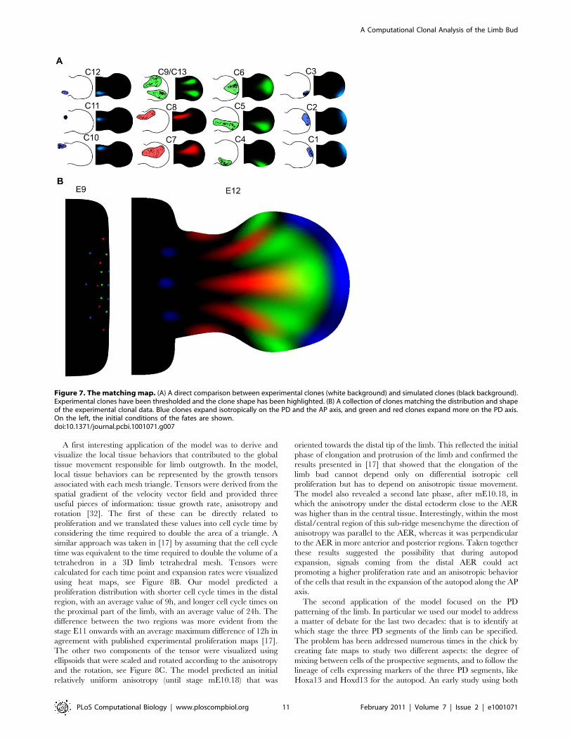
Figure 7. The matching map. (A) A direct comparison between experimental clones (white background) and simulated clones (black background).Experimental clones have been thresholded and the clone shape has been highlighted. (B) A collection of clones matching the distribution and shapeof the experimental clonal data. Blue clones expand isotropically on the PD and the AP axis, and green and red clones expand more on the PD axis.On the left, the initial conditions of the fates are shown.doi:10.1371/journal.pcbi.1001071.g007
A Computational Clonal Analysis of the Limb Bud
PLoS Computational Biology | www.ploscompbiol.org 11 February 2011 | Volume 7 | Issue 2 | e1001071

approaches [7] concluded that the degree of mixing between the
prospective PD segments was low and that the anterior expansion
of the distal marker Hoxa13 was mainly due to growth. In other
words this study suggested that the distal segment was specified
early during development and that it subsequently expanded due
to growth. A similar idea was further developed in [12] where it
was proposed, based on the observation that early fate maps were
almost always confine to a single segment, that the three segments
were specified early in development and that their expansion was
again mainly due to limb growth. This idea became known as the
Early Specification Model. In contrast, a more recent study in
chick [9] concluded that the mixing between zeugopod and
autopod was higher than that between stylopod and zeugopod at
early stages. This together with analysis of Hoxa13 and Hoxa11
expressions suggested that the two more proximal segments were
specified early while the distal segment was specified later during
development. However, another study in chick [8] found no strict
barriers between all the three segments at early stages. Recent
results in mouse [13] also supported a similar view by showing that
cells expressing known markers of three segments were capable of
altering their expression to match the local environments where
they were moved. This supported the idea proposed in [14,15]
that identities were progressively specified over time by active
regulation along the entire limb despite cell transit between the
segments.
Considering some of the controversies mentioned above we
decided to use our model in two ways: firstly to give an estimation
of the degree of mixing along the PD axis, and secondly to
estimate the extent to which limb tissue movement could be
responsible for the expansion of the Hoxd13 domain, one of the
known distal marker of the autopod.
For the first question we used the model to compute a reverse
version of the tissue movement map. This would allow us to start
by marking the three PD segments at the oldest timepoint (E12),
and then work backwards to determine which regions of the young
limb bud could contribute to the 3 segments. Importantly, this is
not equivalent to running a clonal experiment backwards in time.
As in a traditional heat diffusion problem, individual virtual clones
cannot be reverse simulated to discover where they came from. On
the contrary, if a clone was reverse simulated from its final spatial
distribution back to the young limb bud the corresponding region
on the young shape will be proportionally larger than the final
clone. This is clearly the opposite of the normal forward
simulation, which starts with a region much smaller than the final
clone – a single triangle. This distinction is explained in more
detail in Text S3. The purpose of this reverse map is therefore
instead to find the full distribution of possible progenitor regions
for a given final PD zone, e.g. to find the possible distribution of all
zeugopod progenitors at E10. Due to the effective diffusion caused
by cell mixing, the potential progenitor region for a given segment
Figure 8. Derivation of growth tensors. (A) The velocity vector field of the map that best recapitulates limb tissue movement. Velocities havebeen normalized for clarity. (B) A heat map visualizing the expansion rate of each triangle. Red corresponds to high expansion rate (low cell cycle timeof 10h) and blue to low expansion rate (high cell cycle 42h). Average cell cycle times of distal (1/3 of the PD axis from the tip) and proximal parts(remaining 2/3 of the PD axis) are shown for each time point. (C) Ellipses visualizing the anisotropy and rotation of different parts of the tissue. Duringan initial phase of development the anisotropy is relatively uniform (until stage mE10.18) and oriented towards the distal tip of the limb. After thisstage the anisotropy is non-uniformly distributed, and is higher in the region under the influence of the AER. In the central sub-ridge region thedirection of the anisotropy is parallel to the AER, while in more anterior or posterior regions it is perpendicular to the AER.doi:10.1371/journal.pcbi.1001071.g008
A Computational Clonal Analysis of the Limb Bud
PLoS Computational Biology | www.ploscompbiol.org 12 February 2011 | Volume 7 | Issue 2 | e1001071

will always be proportionally larger than the final segment. As an
example, if diffusion was high enough there would be a moment in
the early limb bud when any single cell across the whole bud could
provide descendants contributing to all 3 PD zones of the late bud.
In other words, the progenitor region for any point of the older
limb would be the whole young limb.
The positions of the PD segments at E12 were determined by
the expression of the Sox9 skeletal marker, see Figure 9B. Based
on the degree of cell mixing seen in real clones, our reverse model
revealed the existence of regions having high probability to
contribute to two or three segments at early stages of development
(around stage E10 in Figure 9C) when most of the fate maps
discussed above have been performed. In other words, assuming a
spatially-uniform cell mixing that matches the observed overlaps of
experimental clones, our model clearly suggests that the degree of
mixing between the three PD segments does not allow an early
specification of the PD identities even as late as E10.
For the second analysis of PD patterning we investigated the
possible contribution of tissue movement to the known expansion of
the Hoxd13 distal marker. First we mapped into the model a gene
expression time course of Hoxd13 that was obtained from in-situ
hybridization at 7 different developmental stages, see Figure 10A.
This was done by staging each limb with the morphometric staging
system presented in [28] and by mapping the domain of expression
into the correspondent time point of the model. Secondly, we used
the model to expand or shrink each experimental domain of
expression into the following or the previous experimental time
point, see Figure 10B,C. By computing the difference between the
predicted and the experimental domains we were able to disentangle
the active regulation of Hoxd13 from the underlying tissue
movement. Our model showed that there were periods of growth
during which the change in Hoxd13 domain was fairly consistent
with the underlying tissue movements. However, two particular
periods stood out from this trend during which there was strong
active up-regulation of the gene. The first period was from stage
mE10:15 to stage mE10:19, when the Hoxd13 domain undergoes a
quick expansion from the posterior to the anterior part of the limb,
and the second period was from stage mE11:1 to mE11:18, when the
gene was up-regulated proximally. Interestingly, these phases
seemed to correlate well with (a) the up-regulation of some of the
FGFs expressed by the AER that have been described to expand
from the posterior to anterior part of the distal ectorderm in an initial
phase around E10.5, and (b) a later phase when FGFs expression is
up-regulated around stage E11:5. These observations also fitted with
the model proposed in [14] where FGF signaling was proposed as a
candidate for the regulation of distal markers like Hoxa13.
In conclusion, our model predicts that the degree of mixing
observed in mouse is too high to support the Early Specification
Model as a realistic description of PD region specification.
Moreover we have also shown that the expansion of the Hoxd13
domain, one of the genes proposed as a distal marker of the limb,
cannot be explained considering tissue movement only but has to
involve active up-regulation in at least two distinct phases of the
development.
Discussion
In this study we present a novel computational method which
combines a sequence of experimental 2D limb morphologies and
clonal data to estimate a comprehensive description of the tissue
movement map responsible for limb morphogenesis. We present a
mouse clonal analysis of early hind limb development and show
how this allows us to estimate a 2D descriptive model of limb
outgrowth that fits the experimental data. In practice, our
approach is a reverse-engineering method. It is important to note
that the spring analogy algorithm is used as a convenient tool for
creating a variety of different hypothetical growth maps, but is not
employed to represent the mechanical properties of the tissue.
A major advantage of our model over previous fate maps is the
resulting comprehensive prediction of tissue movements over time
and space. Previously, the behavior of a point of tissue had to be
inferred by manual comparison to its closest experimental clone.
Figure 9. PD segments progenitors. (A) A reverse tissue movement map was calculated in order to identify the progenitor regions for the threePD segments. In the graphs, the stylopod is highlighted in red, the zeugopod in green and the autopod in blue. (B) On the top, the initial position ofthe three PD segments is specified as shown by an in situ hybridization at stage E12 of the Sox9 skeletal marker, on the bottom. (C) Graphs showingthe retrospective probability to belong to the three segments along the proximal distal axis. The regions having a high probability to belong to morethan one segment are highlighted with diagonal black lines.doi:10.1371/journal.pcbi.1001071.g009
A Computational Clonal Analysis of the Limb Bud
PLoS Computational Biology | www.ploscompbiol.org 13 February 2011 | Volume 7 | Issue 2 | e1001071

By contrast, in our new map the movement of every piece of tissue
is described numerically across the whole period of development.
A related advantage is the temporal accuracy – the state of any
hypothetical clone can be predicted at any intermediate time point
– not only at the beginning or end of a virtual clonal experiment.
The spatio-temporal comprehensiveness of the model gives it the
power to make more concrete predictions about PD patterning.
To the best of our knowledge, this is the first comprehensive 2D
model of limb outgrowth derived from experimental data.
Many aspects of our clonal analysis agree with previous results
in mouse [11] and with fate maps in chick [9], in particular that
clones expand across one or two PD segments but never span
across the whole PD axis of the limb. By measuring the degree of
overlap between clones at different PD position we found that
clones spanning the zeugopod had a higher degree of overlap – in
fact not a single zeugopod-restricted clone was found. A
quantification of the ratio between AP and PD clone lengths
highlighted a range of behaviors, but which could be broadly split
into two type: isotropic clones on the distal and proximal part of
the limb, and anisotropic clones in the bulk of the tissue showing
greater PD length than AP length (Figure 3). Interestingly, in
contrast to fate maps in chick [8,9], we found that some distal
clones expanded more on the AP axis than the PD axis (e.g. C2 in
Figure 5A). This was also reflected in the fitting of the hypothetic
growth maps to the clonal data. The map which fitted best (Map6)
displayed specific features regarding AP and PD growth: along the
PD axis it was one of the maps with a distally-restricted PD
elongation. On its own, this information would appear to
contradict the knowledge that proliferation rates are highest
distally, however Map6 was also the one with a strong distal
‘‘fanning-out’’ movement along the AP axis (central row in
Figure 4B). This compensates the low PD expansion resulting in a
strong AP-oriented anisotropy, such that predicted proliferation
rates are maintained at high levels in this region (see Figure 8).
Interestingly, although this feature may be stronger in mouse than
chick (resulting in a wider mouse autopod) recent reports have
suggested that the AP expansion of the chick and gecko autopod
could be driven at least in part by AP-oriented cell divisions [33].
Taking advantage of our computer model we can calculate the
growth tensors directly revealing the AP anisotropy of the distal
tissue. However, the tensors also show that tissue movements of
the most anterior and the most posterior regions of the sub-ridge
mesenchyme are perpendicular to the AER, rather than parallel
(Figure 8C). This is an unexpected observation that will require
more attention in future studies.
Another interesting observation regards the general construc-
tion of our model. By representing the local density of labeled cells
as a probability distribution which can diffuse through a smoothly
deforming mesh, we shows that biologically-realistic tissue
movements can be captured through the combination of
anisotropic velocity vector field, with isotropic diffusion. This
could suggest that the cellular properties which govern mixing,
such as cell-cell adhesion, may not themselves display any cell
polarity. In other words, it is theoretically plausible that cells are
subject to two types of activity: directional movements (such as
oriented cell divisions or convergent extension) which are
responsible for the tissue-level shape changes, and non-directional
cell mixing. However, in reality, alternative scenarios may also be
equally compatible with our model. For example, it is likely that
oriented movements naturally lead to the intercalation and
therefore to the mixing of cells, such that directional movement
and cell mixing cannot be conceptually uncoupled.
Figure 10. Hoxd13 domain expansion. (A) Top row: a sequence of 7 in-situ hybridizations of Hoxd13 with corresponding stage given by themorphometric staging system [17]. Bottom row: the thresholded gene expressions (limb with white background) are mapped into the triangularmeshes of the model (limb with black background). (B) A set of distinct simulations (gray rectangles) showing how the gene expression domains ofeach time point would change if only passively carried along by tissue movements, i.e. with no active cellular up-regulation. (C) A similar set ofsimulations, but this time in reverse for each time point. (D) Differences between the experimental patterns and the ‘‘growth-only’’ simulated patternsin the correspondent column. The green regions are predicted to be up-regulated and the magenta regions to be down-regulated. This indicates thatthe Hoxd13 domain expansion requires active up-regulation on the anterior part around stage mE10.19 (phase 1) and on the proximal part aroundsage mE11:18 (phase 2).doi:10.1371/journal.pcbi.1001071.g010
A Computational Clonal Analysis of the Limb Bud
PLoS Computational Biology | www.ploscompbiol.org 14 February 2011 | Volume 7 | Issue 2 | e1001071

Finally, we used the model to clarify the relation between mouse
limb tissue movement and the existing PD patterning hypothesis.
Firstly we showed, by using a reverse version of the model, that there
is a considerable degree of mixing between the progenitors of the
three PD segments (Figure 9). In contrast to the Early Specification
Model, our model predicts that at early stages there are regions
where cells have a high probability to contribute to more than one
PD segment. Secondly we showed, by mapping a time course of
Hoxd13 expression in the model, that the expansion of the Hoxd13
domain cannot be explained only by tissue movement but requires
active gene regulation, Figure 10. The model gave specific
predictions of the type of spatial and temporal active regulation of
Hoxa13 required suggesting, as proposed in [14], that distal markers
could be under the control of the FGF signaling coming from the
AER. Taken together these two results prove that limb growth
modeling is a valuable resource to extract maximum information
from clonal data and to make specific predictions about the spatio-
temporal dynamic of limb morphogenesis.
To conclude, the software that we developed will allow us to
easily integrate, inside a realistic 2D model of limb growth,
numerical simulations of gene regulatory networks and morpho-
gen gradients taking a big step forward in the study of limb
development by using a systems biology approach.
Materials and Methods
Ethics statementAll animals were handled in strict accordance with good animal
practice as defined by the relevant national and/or local animal
welfare bodies, and all animal work was approved by the
appropriate committee.
Clonal dataThe clonal data was produced using the tamoxifen inducible
Cre-line presented in [11]. Lineage tracing at clonal resolution was
obtained by injecting low dose of tamoxifen (0.10mg) to reduce the
probability of polyclonal origin as described in [11]. Female
pregnant females were injected at approximately 8 days pf. and
embryos were extracted at 12 pf. LacZ clone staining was
performed as described in [34] and embryos were post-fixed in 4%
para-formaldehyde (PFA) and stored in 80% glycerol, 4% PFA.
Limb morphologies72 limb morphologies were extracted from an extended version
of the standard morphological trajectory presented in [28]. Each
limb morphology was represented by an array of curvature values
that were averaged from more than 600 outlines of real limb buds
at different stages. We geometrically reconstructed 72 limb shapes
from the standard morphological trajectory and added an artificial
body of 150|610mm to each shape, see Figure S1. We thus
spatially discretized each of the limb bud shapes using the
unstructured triangular mesh generator presented in [35]. The
meshes used to build the 9 tissue movement maps in Figure 4 were
obtained with an element length of 8mm and the finer version of
the meshes in Figure S2 with an element length of 6mm.
Gene expression dataThe Hoxd13 gene expression time course in Figure 10 and the
Sox9 expression in Figure 3 were made using C57Bl/6J mouse
embryos, fixed in 4%PFA and dehydrated into MetOH. Whole
Mount In situ hybridizations were stained using NBT/BCIP and
performed using a Hoxd13 antisense probe, kindly provided by
Denis Duboule, and a Sox9 antisense probe.
Virtual tissue movment mapsSoftware to generate the virtual tissue movement maps was
written in Java and used the free visualization library vtk [36] to
implement the graphical user interface that allowed the user to
specify the boundary control splines. Virtual tissue movement maps
were stored on a re-usable data structure called MorphoMovie that
was defined by a series of velocity vector fields and a series of
triangle interpolation maps, one for each triangular mesh in the
sequence. We developed a generic partial differential equation
solver that was able to simulate virtual clones on a given
MorphoMovie. The solver used an Euler method for time
discretization and a Finite Volume Method [37,38] on unstruc-
tured triangular meshes for the space discretization.
Supporting Information
Figure S1 Standard morphological trajectory. The 72 experi-
mental limb bud morphologies describing mouse hind-limb
development from stage E9 to stage E12.
Found at: doi:10.1371/journal.pcbi.1001071.s001 (0.33 MB PDF)
Figure S2 Analysis of the clonal data (PD and AP length
measurement). The clonal data that was generated using the
tamoxifen inducible CRE transgenic mouse line. Clones are divided
in two groups: isotropically expanding clones and an-isotropically
expanding clones. The PD and AP clone lengths relative to the
maximum PD and AP length of the limb are measured. Colored
triangles represent the AP and PD clone expansion.
Found at: doi:10.1371/journal.pcbi.1001071.s002 (1.17 MB PDF)
Figure S3 Proliferation patterns of the maps shown in Figure 4.
The proliferation patterns of the 9 virtual tissue movement maps
in Figure 4. Triangle expansion rate are converted to cell cycle
time and are visualized by using a heat map, red corresponds to
low cell cycle times (11h) and blue to high cell cycle times (43h).
Found at: doi:10.1371/journal.pcbi.1001071.s003 (0.40 MB PDF)
Figure S4 Experimental clone registration. The collection of 13
experimental clones that were mapped into the last triangular
mesh of the sequence (stage E12).
Found at: doi:10.1371/journal.pcbi.1001071.s004 (0.66 MB PDF)
Figure S5 Clone scores of the tissue movement maps in Figure 4.
For each of the 9 virtual tissue movement maps, the collection of
virtual clones that best matched the 13 experimental clones.
Virtual clones are shown with colored contour lines and
experimental clones are shown in white color. The text in white
color is the virtual clone score. Finally, a bar diagram summarizing
the clone scores.
Found at: doi:10.1371/journal.pcbi.1001071.s005 (1.68 MB PDF)
Text S1 Description of the tissue movement maps in Figure 4. A
description of the spline curves and stiffness distributions used to
generate the 9 virtual tissue movement maps in Figure 4.
Found at: doi:10.1371/journal.pcbi.1001071.s006 (0.04 MB PDF)
Text S2 Simulation with a refined triangular mesh. The 13
virtual clone positions in Map6 that best matched the experimen-
tal data were used to simulate virtual clones on a version of Map6
with a refined mesh.
Found at: doi:10.1371/journal.pcbi.1001071.s007 (0.46 MB PDF)
Text S3 Forward and backward maps. A description of the
different information that can be extrapolated from a virtual tissue
movement map: fate maps vs progenitor regions. The PD segment
progenitor prediction shown in Figure 9 is also recalculated by
using Map6 without additional diffusion.
Found at: doi:10.1371/journal.pcbi.1001071.s008 (1.00 MB PDF)
A Computational Clonal Analysis of the Limb Bud
PLoS Computational Biology | www.ploscompbiol.org 15 February 2011 | Volume 7 | Issue 2 | e1001071

Video S1 Mesh deformation video. Part of the sequence of
triangular meshes that was derived from the experimental limb
bud morphologies. Each mesh is deformed to match the next mesh
in the sequence from which the simulation continues.
Found at: doi:10.1371/journal.pcbi.1001071.s009 (5.46 MB AVI)
Video S2 Virtual fate map video. A video showing a virtual fate
map. The spatial probability distribution of the fate is colored with
a heat map, red represents a high probability and blue a low
probability. A discrete number of triangle-interpolation steps can
be appreciated in the video.
Found at: doi:10.1371/journal.pcbi.1001071.s010 (3.21 MB AVI)
Video S3 Video of the simulation in Figure 7B. A video showing
a number of clones that match the distribution and shape of the
experimental clonal data. Blue clones expand isotropically on the
AP and the PD axis, red and green clones expand more on the PD
axis.
Found at: doi:10.1371/journal.pcbi.1001071.s011 (2.70 MB AVI)
Acknowledgments
We wish to thank Laura Quintana for the photos of the Hoxd13 in-situs
patterns, Jelena Raspopovic for the Sox9 in-situ, Bernd Boehm for help
with the limb bud shapes and Jim Swoger for the useful discussion.
Author Contributions
Conceived and designed the experiments: LM CGA MST JS. Performed
the experiments: LM CGA. Analyzed the data: LM JS. Contributed
reagents/materials/analysis tools: LM. Wrote the paper: LM JS.
References
1. Yang Y (2009) Growth and patterning in the limb: Signaling gradients make the
decision. Development 2: pe3.2. Tickle C (2003) Patterning systems-from one end of the limb to the other. Dev
Cell 4: 449–458.
3. Tickle C (2006) Making digit patterns in the vertebrate limb. Nat Rev Mol CellBiol 7: 45–53.
4. Zeller R, Lopez-Rıos J, Zuniga A (2009) Vertebrate limb bud development:moving towards integrative analysis of organogenesis. Nat Rev Genet 10:
845–858.5. Benazet J, Zeller R (2009) Vertebrate limb development: moving from classical
morphogen gradients to an integrated 4-dimensional patterning system. Cold
Spring Harb Perspect Biol 1: a001339.6. Towers M, Tickle C (2009) Growing models of vertebrate limb development.
Development 136: 179–190.7. Vargesson N, Clarke JD, Vincent K, Coles C, Wolpert L, et al. (1997) Cell fate
in the chick limb bud and relationship to gene expression. Development 124:
1909–1918.8. Pearse R, Scherz P, Campbell J, Tabin C (2007) A cellular lineage analysis of the
chick limb bud. Dev Biol 310: 388–400.9. Sato K, Koizumi Y, Takahashi M, Kuroiwa A, Tamura K (2007) Specification
of cell fate along the proximal-distal axis in the developing chick limb bud.Development 134: 1397–1406.
10. Muneoka K, Wane N, Bryant S (1989) Mammalian limb bud development: In
situ fate maps of early hindlimb buds. J Exp Zool 249: 50–54.11. Arques C, Doohan R, Sharpe J, Torres M (2007) Cell tracing reveals a
dorsoventral lineage restriction plane in the mouse limb bud mesenchyme.Development 134: 3713–3722.
12. Dudley A, Ros M, Tabin C (2002) A re-examination of proximodistal patterning
during vertebrate limb development. Nature 418: 539–544.13. Wyngaarden L, Sevan H (2008) Plasticity of proximal-distal cell fate in the
mammalian limb bud. Dev Biol 313: 225–233.14. Mercader N, Leonardo E, Piedra M, Martinez A, Ros A, et al. (2000) Opposing
ra and fgf signals control proximodistal vertebrate limb development through
regulation of meis genes. Development 127: 3961–3970.15. Tabin C, Wolpert L (2007) Rethinking the proximodistal axis of the vertebrate
limb in the molecular era. Development 21: 1433–1442.16. Summerbell D, Lewis J, Wolpert L (1973) Positional information in chick limb
morphogenesis. Nature 244: 492–496.17. Bohm B, Lesnicar-Pucko G, Sharpe J (2010) The role of spatially controlled cell
proliferation in limb bud morphogenesis. PLoS Biol 8: e1000420.
18. Li S, Muneoka K (1999) Cell migration and chick limb development:Chemotactic action of fgf-4 and the aer. Dev Biol 211: 335–347.
19. Wyngaarden L, Sevan H (2010) Oriented cell motility and division underlieearly limb bud morphogenesis. Development 8: e1000420.
20. Boot MJ, Westerberg C, Sanz-Ezquerro J, Cotterell J, Schweitzer R, et al. (2008)
In vitro whole-organ imaging: 4d quantification of growing mouse limb buds.Nat Methods 5: 609–612.
21. Colas J, Sharpe J (2009) Live optical projection tomography. Organogenesis 5:
129–134.
22. Rolland-Lagan A, Bangham J, Coen E (2003) Growth dynamics underlying
petal shape and asymmetry. Nature 422: 161–163.
23. Rolland-Lagan AG, Coen E, Impey S, Bangham J (2005) A computational
method for inferring growth parameters and shape changes during development
based on clonal analysis. J Theor Biol 232: 157–177.
24. Morishita Y, Iwasa Y (2008) Growth based morphogenesis of vertebrate limb
bud. J Theor Biol 70: 1957–1978.
25. Dillon R, Othmer HG (1999) A mathematical model for outgrowth and spatial
patterning of the vertebrate limb bud. J Theor Biol 197: 295–330.
26. Ede D, Law J (1969) Computer simulation of vertebrate limb morphogenesis.
Nature 221: 244–248.
27. Gros JJ, abdHu, Vinegoni C, Feruglio P, Weissleder R, Tabin C (2010) Wnt5a/
jnk and fgf/mapk pathways regulate the cellular events shaping the vertebrate
limb bud. Curr Biol 20: 1993–2002.
28. Bohm B, Rautschka M, Raspopovic J, Quintana L, Jan Z, et al. (In press.) A
landmark-free morphometric staging system for the mouse limb bud.
Development.
29. FJ B (2000) Considerations on the spring analogy. Int J Numer Meth Fl 32:
647–668.
30. Van Loon R, Anderson PD, Van de Vosse FN, Sherwin SJ (2007) Comparison
of various fluid-structure interaction methods for deformable bodies. Comput
Struct 85: 833–843.
31. Chaniotis A, Poulikakos D, Koumoutsakos P (2002) Remeshed smoothed
particle hydrodynamics for the simulation of viscous and heat conducting flows.
J Comput Phys 182: 67–90.
32. Coen E, Rolland-Lagan A, Matthews M, Bangham J, Prusinkiewicz P (2004)
The genetics of geometry. Proc Natl Acad Sci U S A 101: 4728–4735.
33. Sato K, Seki R, Noro M, Yokoyama H, Tamura K (2010) Morphogenetic
change of the limb bud in the hand plate formation. J Exp Zool B Mol Dev Evol
314B: 539–551.
34. Torres M (1998) The use of embryonic stem cells for the genetic manipulation of
the mouse. Curr Top Dev Biol 36: 99–114.
35. Geuzaine C, Remacle J (2009) Gmsh: a three-dimensional finite element mesh
generator with built-in pre- and post-processing facilities. Int J Numer Meth Eng
79: 1309–1331.
36. Schroeder W, Martin K, Lorensen B (2006) The Visualization Toolkit An
Object-Oriented Approach To 3D Graphics, 4th Edition Kitware, Inc.
publishers.
37. LeVeque R (2005) Numerical Methods for Conservation Laws, 2nd ed.
Birkhauser Basel.
38. Eymard R, Gallouet T, Herbin R (2000) The finite volume method. Handbook
of Numerical Analysis 7: 713–1020.
A Computational Clonal Analysis of the Limb Bud
PLoS Computational Biology | www.ploscompbiol.org 16 February 2011 | Volume 7 | Issue 2 | e1001071


![Characterization of Mouse Switch Variant Antibodies by ... · [7]. Peptide mapping also has been performed for the characterization of a recombinant humanized mono- clonal antibody](https://static.fdocuments.net/doc/165x107/5e1fa5318878e229647fc833/characterization-of-mouse-switch-variant-antibodies-by-7-peptide-mapping.jpg)