A COMPARISON OF RANKING METHODS FOR NORMALIZING SCORES ...

A COMPARISON OF RANKING METHODS

FOR NORMALIZING SCORES

by

SHIRA R. SOLOMON

DISSERTATION

Submitted to the Graduate School

of Wayne State University,

Detroit, Michigan

in partial fulfillment of the requirements

for the degree of

DOCTOR OF PHILOSOPHY

2008

MAJOR: EVALUATION AND RESEARCH

Approved by:

______________________________ Advisor Date

______________________________

______________________________

______________________________

UMI Number: 3303509

33035092008

Copyright 2008 bySolomon, Shira R.

UMI MicroformCopyright

All rights reserved. This microform edition is protected against unauthorized copying under Title 17, United States Code.

ProQuest Information and Learning Company 300 North Zeeb Road

P.O. Box 1346 Ann Arbor, MI 48106-1346

All rights reserved.

by ProQuest Information and Learning Company.

© COPYRIGHT BY

SHIRA R. SOLOMON

2008

All Rights Reserved

ii

DEDICATION

To my maternal grandmother, Mary Karabenick Brooks, whose love of art,

literature, and music has gone hand in hand with her concern for social welfare. To

my paternal grandmother, Frances Hechtman Solomon, who played the cards she

was dealt with style and wit.

iii

ACKNOWLEDGEMENTS

A dissertation is largely a solitary project, yet it builds on the contributions of

many. I have been standing on many shoulders.

First, I would like to thank my major advisor, Professor Shlomo Sawilowsky,

whose grand passion for argument made him someone I could relate to, and made

statistics seem worth doing. Dr. Sawilowsky has been generous with his time,

technical help, and the spirited exegeses that put this discipline in its true human

context.

Professors Gail Fahoome, Judith Abrams, and Leonard Kaplan have

brought a great deal to this dissertation and to my graduate experience. Dr.

Fahoome has been an excellent teacher, consistently insightful and reassuringly

low-key. I lucked into meeting Dr. Abrams through my research assistantship with

the medical school. Her assistance and advice have been invaluable. Dr. Kaplan

paid me the extraordinary compliment of joining my committee on the brink of his

retirement. I am indebted to each of these professors for their intellectual integrity

and their simple kindness.

I regret the untimely passing of Professor Donald Marcotte, who would have

been proud to see this dissertation completed. Dr. Marcotte provided a wonderful

initiation into the world of statistics, with his perennial admonition that the faster

you can solve problems, the more time you have to enjoy life.

When it came time to apply for this doctoral program, I reached out to the

professors who knew me best. I did not find them, in the end, in the ideological

combat zone of my master’s program or in the artful arena of my literary studies. I

iv

found them within the seminary walls, among the rabbis and professors who taught

me Talmud. Studying Talmud helped me to stop thinking so much and just learn.

For accomplishing this ingenious feat, and for supporting all my educational

adventures, I would like to thank Professor David Kraemer, Rabbi Leonard Levy,

and Professor Mayer Rabinowitz.

To Bruce Chapman, the teacher who forced inspiration to the forefront,

where it belongs: Here’s to you, Captain. To my great friends, Regina DiNunzio,

Tom Kilroe, Katy Potter, and Deborah Mougoue, who keep me on my toes.

My parents, Carole and Elliot Solomon, have been the staunchest

advocates of this reckless leap. Their unrelenting curiosity and unvarnished

pleasure in my pursuits has given me strength. And Mark Sawasky, my constant

friend and fan and love, becomes a bigger mensch every day.

v

TABLE OF CONTENTS

DEDICATION ............................................................................................................ ii

ACKNOWLEDGEMENTS ........................................................................................ iii

LIST OF TABLES.................................................................................................... vii

LIST OF FIGURES................................................................................................... ix

CHAPTERS

CHAPTER 1 – Introduction...................................................................... …...1

Research problem................................................................................5

Importance of the problem...................................................................6

Assumptions and limitations ................................................................7

Definitions ............................................................................................8

CHAPTER 2 – Literature review...................................................................10

Mental testing and the normal distribution .........................................10

Norm-referencing and the T score .....................................................11

Nonnormality observed ......................................................................13

Statistical considerations ...................................................................14

Standardizing transformations ...........................................................21

Approaches to creating normal scores ..............................................28

CHAPTER 3 – Methodology.........................................................................32

Programming specifications...............................................................33

Sample sizes......................................................................................33

Number of Monte Carlo repetitions ....................................................33

Achievement and psychometric distributions.....................................33

vi

Presentation of results .......................................................................34

CHAPTER 4 – Results .................................................................................43

CHAPTER 5 – Conclusion............................................................................89

Discussion..........................................................................................92

Moment 1—mean ..............................................................................92

Moment 2—standard deviation ..........................................................92

Moment 3—skewness........................................................................95

Moment 4—kurtosis ...........................................................................95

Recommendations.............................................................................96

REFERENCES........................................................................................................98

ABSTRACT ...........................................................................................................110

AUTOBIOGRAPHICAL STATEMENT...................................................................112

vii

LIST OF TABLES

Table 1. Differences among Ranking Methods in Attaining Target Moments .........25

Table 2. Smooth Symmetric—Accuracy of T Scores on Means..............................45

Table 3. Smooth Symmetric—Accuracy of T Scores on Standard Deviations ........46

Table 4. Smooth Symmetric—Accuracy of T Scores on Skewness ........................47

Table 5. Smooth Symmetric—Accuracy of T Scores on Kurtosis ...........................48

Table 6. Discrete Mass at Zero—Accuracy of T Scores on Means.........................49

Table 7. Discrete Mass at Zero—Accuracy of T Scores on Standard Deviations ...50

Table 8. Discrete Mass at Zero—Accuracy of T Scores on Skewness ...................51

Table 9. Discrete Mass at Zero—Accuracy of T Scores on Kurtosis.......................52

Table 10. Extreme Asymmetric, Growth—Accuracy of T Scores on Means ...........53

Table 11. Extreme Asymmetric, Growth—Accuracy of T Scores on Standard

Deviations................................................................................................................54

Table 12. Extreme Asymmetric, Growth—Accuracy of T Scores on Skewness......55

Table 13. Extreme Asymmetric, Growth—Accuracy of T Scores on Kurtosis .........56

Table 14. Digit Preference—Accuracy of T Scores on Means….............................57

Table 15. Digit Preference—Accuracy of T Scores on Standard Deviations...........58

Table 16. Digit Preference—Accuracy of T Scores on Skewness...........................59

Table 17. Digit Preference—Accuracy of T Scores on Kurtosis ..............................60

Table 18. Multimodal Lumpy—Accuracy of T Scores on Means.............................61

Table 19. Multimodal Lumpy—Accuracy of T Scores on Standard Deviations .......62

Table 20. Multimodal Lumpy—Accuracy of T Scores on Skewness .......................63

Table 21. Multimodal Lumpy—Accuracy of T Scores on Kurtosis...........................64

viii

Table 22. Mass at Zero with Gap—Accuracy of T Scores on Means......................65

Table 23. Mass at Zero with Gap—Accuracy of T Scores on Standard

Deviations................................................................................................................66

Table 24. Mass at Zero with Gap—Accuracy of T Scores on Skewness ................67

Table 25. Mass at Zero with Gap—Accuracy of T Scores on Kurtosis....................68

Table 26. Extreme Asymmetric, Decay—Accuracy of T Scores on Means.............69

Table 27. Extreme Asymmetric, Decay—Accuracy of T Scores on Standard

Deviations................................................................................................................70

Table 28. Extreme Asymmetric, Decay—Accuracy of T Scores on Skewness .......71

Table 29. Extreme Asymmetric, Decay—Accuracy of T Scores on Kurtosis...........72

Table 30. Extreme Bimodal—Accuracy of T Scores on Means...............................73

Table 31. Extreme Bimodal—Accuracy of T Scores on Standard Deviations .........74

Table 32. Extreme Bimodal—Accuracy of T Scores on Skewness .........................75

Table 33. Extreme Bimodal—Accuracy of T Scores on Kurtosis ............................76

Table 34. Deviation from Target, Summarized by Moment, Sample Size, and

Distribution ..............................................................................................................90

Table 35. Winning Approximations, Summarized by Moment, Sample Size, and

Distribution ..............................................................................................................91

ix

LIST OF FIGURES

Figure 1. Comparison of Scores in a Normal Distribution .........................................3

Figure 2. Distribution of T Scores Using Blom’s Approximation: Good fit on all four

moments .................................................................................................................26

Figure 3. Distribution of T Scores Using Blom’s Approximation: Poor fit on second

and third moments ..................................................................................................27

Figure 4. Distribution of T Scores Using Blom’s Approximation: Poor fit on fourth

moment ...................................................................................................................28

Figure 5. Achievement: Smooth Symmetric ............................................................35

Figure 6. Achievement: Discrete Mass at Zero .......................................................36

Figure 7. Achievement: Extreme Asymmetric, Growth............................................37

Figure 8. Achievement: Digit Preference.................................................................38

Figure 9. Achievement: Multimodal Lumpy .............................................................39

Figure 10. Psychometric: Mass at Zero with Gap....................................................40

Figure 11. Psychometric: Extreme Asymmetric, Decay...........................................41

Figure 12. Psychometric: Extreme Bimodal ............................................................42

Figure 13. Smooth Symmetric: Power curve for deviation range of standard

deviation..................................................................................................................78

Figure 14. Smooth Symmetric: Power curve for deviation range of kurtosis ...........78

Figure 15. Discrete Mass at Zero: Power curve for deviation range of standard

deviation..................................................................................................................79

Figure 16. Discrete Mass at Zero: Power curve for deviation range of kurtosis ......79

x

Figure 17. Extreme Asymmetric, Growth: Power curve for deviation range of

standard deviation ...................................................................................................80


kurtosis ....................................................................................................................80

Figure 19. Digit Preference: Power curve for deviation range of standard

deviation..................................................................................................................81

Figure 20. Digit Preference: Power curve for deviation range of kurtosis................81

Figure 21. Multimodal Lumpy: Power curve for deviation range of standard

deviation..................................................................................................................82

Figure 22. Multimodal Lumpy: Power curve for deviation range of kurtosis ............82

Figure 23. Mass at Zero with Gap: Power curve for deviation range of standard

deviation..................................................................................................................83

Figure 24. Mass at Zero with Gap: Power curve for deviation range of kurtosis .....83

Figure 25. Extreme Asymmetric, Decay: Power curve for deviation range of

standard deviation ...................................................................................................84


kurtosis ....................................................................................................................84

Figure 27. Extreme Bimodal: Power curve for deviation range of standard

deviation..................................................................................................................85

Figure 28. Extreme Bimodal: Power curve for deviation range of kurtosis ..............85


deviation with inclusion of large sample sizes .........................................................87

xi

Figure 30. Digit Preference: Power curve for deviation range of standard deviation

with inclusion of large sample sizes ........................................................................87

Figure 31. Mass at Zero with Gap: Power curve for deviation range of kurtosis with

inclusion of large sample sizes................................................................................88

1

CHAPTER 1

INTRODUCTION

To those who believe that “the purpose of data analysis is to analyze data better”

it is clearly wise to learn what a procedure really seems to be telling us about.

(J. W. Tukey, 1962)

Standardized tests can be used to determine aptitude or achievement

(Thorndike, 1982). Whether the goal of a test is to measure differences in ability,

personality, or mastery of a subject, it is necessary to analyze individual scores

relative to others in the group and also to analyze group scores relative to other

group scores (Angoff, 1971; AERA, APA, & NCME, 1999; Netemeyer, Bearden,

and Sharma, 2003). Scores are ultimately interpreted according to the purpose of

the test. For example, academic aptitude tests are likely to be interpreted

competitively, with high performing students favored for scholarships or admission

to selective programs and low performing students targeted for remediation.

Achievement tests are typically interpreted in the light of performance benchmarks

and used to measure the adequacy of teaching methods or school performance.

Analysis for either purpose requires a frame of reference for the interpretation of

raw scores (Aiken, 1994).

Standardization and normalization are two ways of defining the frame of

reference for a distribution of test scores. Both types of score conversions, or

transformations, mathematically modify raw score values (Osborne, 2002). The

defining feature of standard scores is that they use standard deviations to describe

scores’ distance from the mean, thereby creating equal units of measure within a

2

given score distribution. Standard scores may be modified to change the scale’s

number system (Angoff, 1984), but unless distributions of standard scores are

normalized, they will retain the shape of the original score distribution. Therefore,

standardization may enable effective analysis of individual scores within a single

test, but it does not lead to meaningful comparisons between tests.

Normalization surmounts this limitation by equalizing the areas under the

curve that correspond with scores’ successive intervals along the curve.

Normalization is considered a type of area transformation because it “redefines the

unit separations”(Angoff, 1984, p.36), changing the shape of the distribution itself.

Normalization has two great strengths, the first of which is shared by

standardization: 1) it transforms ordinal scales into continuous scales, which are

mathematically tractable; and 2) it superimposes a normal curve onto nonnormal

distributional shapes, allowing for between-test comparisons.

Normal scores may be scaled to make them easier to interpret. For

example, the formula T = 10Z + 50 replaces normalized standard scores with T

scores, which have a mean of 50 and a standard deviation of 10. Many normal

score systems are assigned means and standard deviations that correspond with

the T score. For example, the College Entrance Board’s Scholastic Aptitude Test

(SAT) Verbal and Mathematical sections are scaled to a mean of 500 and a

standard deviation of 100. Thus, T scores fall between 20 and 80 and SAT scores

fall between 200 and 800. Other normalized standard scores include normal curve

equivalent (NCE) scores, which have a mean of 500, a standard deviation of 21,

and a score range of 1-99; Wechsler scales, which have a mean of 100, a

3

standard deviation of 15, and a 95% score range of 55-145; and stanines, which

have a mean of 5, a standard deviation of 2, and a finite score range of 1-9.

Figure 1. Comparison of scores in a normal distribution. (Adapted from Test

Service Bulletin of The Psychological Corporation, 1955)

The first step in the process of converting raw scores into T scores or other

scaled, normal scores is a ranking of the raw scores according to their relative

placement on the unit normal distribution. This means that the raw scores will no

longer be used to characterize the test score distribution. Instead, raw scores will

be replaced by an estimate of their normal probability deviates. Whereas raw

scores originally refer to individual coordinates, they are transformed to become

components in the two dimensional spaces, or categories, which comprise the

area under the normal distribution. Once these normal probability deviates, or Z

4

scores, are obtained, the desired mean and standard deviation are applied. In the

case of T scores, Z scores are multiplied by 10 and assigned a mean of 50.

A number of ranking methods that improve the accuracy and efficiency of

the traditional percentile method have been developed in the last 60 years. These

ranking methods are sometimes referred to as proportion estimates because they

approximate where the ordinal scores fall along a normal distribution and how

much of the corresponding area under the curve the ranked, cumulative

proportions occupy. The most prominent of these procedures, based on their

inclusion in widely used computer statistical software (e.g., SPSS, 2006) are those

attributed to Van der Waerden (1952, 1953a, 1953b; Lehmann, 1975), Blom

(1958), and Tukey (1962), and the Rankit procedure (Ipsen & Jerne, 1944; Bliss,

1956). These proportion estimates have been explored to various degrees in the

context of hypothesis testing, where the focus is necessarily on the properties of

these estimates in the tails of a distribution. In the context of standardized testing,

however, the body of the distribution—that is, the 95% of the curve that lies

between the tails—is the focus. To date, there has been no empirical comparison

of these ranking methods as they apply to standardized testing.

When normalizing standard scores, practitioners need to know the

comparative effects of their selected ranking method on the transformed score

outcomes. Specifically, during the transformation of Z scores into T scores, the

practitioner would benefit from knowing each method’s potential accuracy and how

frequently it is capable of attaining a specific level of accuracy. Conversely, each

method’s likely degree and frequency of inaccuracy should be taken into account.

5

For T scores, the criteria for comparing ranking methods are the accuracy and

frequency of random scores’ attainment of a mean of 50 and a standard deviation

of 10. The standard deviation for T scores, alone, is not a useful point of

comparison because it is built on the mean; therefore, its degree of accuracy

derives from that of the mean and cannot be used as an independent reference

point. However, the accuracy of its standard deviation (that is, how nearly and how

frequently it obtains a value of 10) is equally important once the value of the mean

has been shown to be 50.

T scores express only the first and second moments of the distribution,

central tendency (mean) and variability (standard deviation), but they may also be

affected by the third and fourth moments, asymmetry (skewness) and peakedness

(kurtosis). Although each of these ranking methods is designed to produce a unit

normal score distribution, they may not achieve ideal skewness and kurtosis. A

normal curve is perfectly symmetrical, meaning it has zero skew. A kurtosis of

three (3) means the shape of the curve is neither more peaked nor more flat than

the shape of an idealized normal distribution. It is necessary to examine the

skewness and kurtosis of T scores, in addition to their means and standard

deviations, in order to fully evaluate each ranking method’s effectiveness in

normalizing test scores.

Research Problem

Given the importance of transforming Z scores to a scale that preserves a

mean of 50 and a standard deviation of 10, this study aims to empirically

demonstrate the relative accuracy of the Blom, Tukey, Van der Waerden, and

6

Rankit approximations for the purpose of normalizing test scores. It will compare

their accuracy in terms of achieving the T score’s specified mean and standard

deviation and unit normal skewness and kurtosis, among small and large sample

sizes in an array of real, nonnormal distributions. Although this objective is an

applied one, the investigation will benefit the theoretical advancement of area

estimation under the normal distribution.

Importance of the Problem

Standardized test scores, even scores abiding by the familiar T score scale,

are notoriously difficult to interpret (Micceri, 1990). Most test-takers, parents, and

even many educators, would be at a loss to explain exactly what a score of 39, 73,

or 428 means in conventional terms, such as pass/fail, percentage of questions

answered correctly, or performance relative to other test-takers. The matter is

complicated by standard error. Once error is computed and added/subtracted from

a given test score, it reveals a range of possible true scores.

Thus, a standard error of three would produce a range of six scores: it

would show the score 52 to be potentially as low as 49 or as high as 55. This

example assumes that the mean is 50. However, if a different ranking method

produces a mean of 51, the test-taker’s score would be between 50 and 56—or

combining the two methods’ results, between 49 and 56. If yet another method

produces a mean closer to 49, then theoretically, a test-taker’s true score could lie

anywhere between 48 and 56. The potential range of true scores expands with

each alternate method of computing the normalized score. Error is not a fixed

7

quantity; it may vary across computational methods as well as sample sizes and

statistical distributions.

The accuracy, both in terms of degree and frequency, of the four most

visible ranking methods has not been established. Blom, Tukey, Van der Waerden,

and Rankit each contribute a ranking formula that approximates a normal

distribution, given a set of raw scores or nonnormalized standard scores. However,

the formulas themselves have not been systematically compared for their first four

moments’ accuracy in terms of normally distributed data. Nor have they been

compared in the harsher glare of nonnormal distributions, which are prevalent in

the fields of education and psychology (Micceri, 1989). Small samples are also

common in real data and are known to have different statistical properties than

large samples (Conover, 1980). In general, real data can be assumed to behave

differently than data that is based on theoretical distributions, even if these are

nonnormal (Stigler, 1977).

Assumptions and Limitations

A series of Monte Carlo simulations will draw samples of different sizes from

eight different empirically established population distributions. These eight

distributions, though extensive in their representation of real achievement and

psychometric test scores, do not represent all possible distributions that could

occur in educational and psychological testing, or in social and behavioral science

investigations more generally. Nor do the sample sizes represent every possible

increment. However, both the sample size increments and the range of

distributional types are assumed to be sufficient for the purpose of outlining the

8

comparative accuracy and reliability of the ranking methods in real settings.

Although the interpretation of results need not be restricted to educational and

psychological data, similar distributional types may be most often found in these

domains.

Definitions

Z scores Raw scores or random variables that have undergone

the standardizing transformation (X – µ) / σ , where µ is

the mean and σ is the population standard deviation.

Also called unmodified standard scores.

Normal scores Raw scores or standard scores that have undergone a

normalizing transformation such that the ordinal

rankings of scores correspond to their probability

deviates on the unit normal distribution.

T scores Raw scores or standard scores that have undergone

the scaling transformation 10Z +50 , where Z is the

normal probability deviate corresponding to the ordinal

rank of the original raw or standard score.

Proportion estimates Approximation formulas estimating the cumulative

areas under a unit normal distribution that fall below the

ordinal rankings of test scores.

9

Rankit approximation A proportion estimate using the formula (r - 1/2) / n. *

Van der Waerden’s approximation A proportion estimate using the formula

r / (n + 1), where r is the rank, ranging from 1 to n.

Blom’s approximation A proportion estimate using the formula (r - 3/8) / (n +

1/4).

Tukey’s approximation A proportion estimate using the formula (r - 1/3) / (n +

1/3).

Monte Carlo simulation A statistical experiment modeled on a computer that

uses an iterative random sampling process, usually with

replacement of data values, to demonstrate the

behavior of statistical methods under specified

conditions.

* Notation for these four approximation formulas varies in the literature: 1) r is used

interchangeably with i and k; and 2) n is used interchangeably with w.

10

CHAPTER 2

LITERATURE REVIEW

The development of ranking methods stems from two related enterprises:

the psychological effort to measure mental phenomena and the statistical effort to

calculate the area under the unit normal distribution. Knowledge, intellectual ability,

and personality are psychological objects that can only be measured indirectly, not

by direct observation (Dunn-Rankin, 1983). The scales that describe them are

hierarchical—they result in higher or lower scores—but these scores do not

express exact quantities of test-takers’ proficiency or attitudes.

Likert scales, which are ordinal, and multiple choice items, which produce

discrete score scales, result in numbers that are meaningless without purposeful

statistical interpretation (Nanna & Sawilowsky, 1998). Measures with unevenly

spaced increments interfere with the interpretation of test scores against

performance benchmarks, the longitudinal linking of test editions, and the equating

of parallel forms of large-scale tests (Aiken, 1987). They also threaten the

robustness and power of the parametric statistical procedures that are

conventionally used to analyze standardized test scores (Friedman, 1937;

Sawilowsky & Blair, 1992).

Mental Testing and the Normal Distribution

Standardized test scores present a unique set of statistical considerations

because the scoring system may be devised for different purposes. Mehrens and

Lehmann (1987) characterized these purposes as instructional, guidance,

administrative, or research, but admittedly, these purposes often overlap. If the

11

purpose of a test is to discriminate between test-takers’ ability or achievement

levels, the scoring system would create maximum variability between scores. If its

purpose is to evaluate students’ progress toward a specified objective, then the

degree of variability between scores is less relevant. Apart from the natural range

of test-takers’ aptitude, subject-matter proficiency, and range of attitudes or

personality characteristics, a test’s design has a strong influence on its score

distribution.

Norm-Referencing and the T Score

The history of testing is fraught with incorrect distributional assumptions.

According to Angoff (1984), “the assumption underlying the search for equal units

was that mental ability is fundamentally normally distributed and that equal

segments on the base line of a normal curve would pace off equal units of mental

ability”(p.11). McCall (1939) devised the T score scale on this same assumption,

naming it after the educational and psychological measurement pioneers

Thorndike and Terman (Walker & Lev, 1969). McCall derived a normal scale by

randomly selecting individuals from a population that was presumed to be

homogenous, testing them, creating a distribution from their scores, and

transforming their percentile ranks to normal deviate scores with a preassigned

mean of 50 and standard deviation of 10. Today, this method would be considered

appropriate for norm-referencing a test to a target population, but thoroughly

inappropriate for determining any true ability distribution. Although there is no

reason to assume that cognitive phenomena are normally distributed, norm-

12

referencing can be useful for comparing individuals’ performance to others in the

same population.

Even when norming makes correct distributional assumptions, it can be

problematic. Angoff (1971) argued against normative scoring systems that have

built-in, definitional, or inherent meaning. These meanings are liable to be lost over

time or to become irrelevant. Aiken (1994) cautioned that norms can become

outdated even more quickly in certain circumstances: “for example, changes in

school curricula may necessitate restandardizing and perhaps modifying and

reconstructing an achievement test every 5 years or so”(p.78). Furthermore, scales

can function independently of direct representation. For example, inches, pounds,

and degrees Fahrenheit no longer reference their original object for most

Americans, but serve as effective measures nonetheless, due to their familiarity

and reliability. Likewise, the T score owes much of its usefulness to its

longstanding place as the scale of choice.

Despite these arguments, Mehrens and Lehmann (1987) viewed norm-

referencing as the basis for most testing theory and practice. It is “useful in

aptitude testing where we wish to make differential predictions. It is also very

useful to achievement testing”(p.18). They also noted that standardized tests are

often used in both norm-referenced and criterion-referenced contexts; they may be

constructed and interpreted to simultaneously compare a student’s performance

relative to other students in the target test-taking population as well as to evaluate

the student’s absolute knowledge of a subject. Norms may be referenced to

13

national, regional, and local standards; age and grade; mental age; percentiles; or

standard scores that are a function of a specific group’s performance.

Nonnormality Observed

According to Nunnally (1978), “test scores are seldom normally

distributed”(p.160). Micceri (1989) demonstrated the extent of this phenomenon in

the social and behavioral sciences by evaluating the distributional characteristics

of 440 real data sets collected from the fields of education and psychology.

Standardized scores from national, statewide, and districtwide test scores

accounted for 40% of them. Sources included the Comprehensive Test of Basic

Skills (CTBS), the California Achievement Tests, the Comprehensive Assessment

Program, the Stanford Reading tests, the Scholastic Aptitude Tests (SATs), the

College Board subject area tests, the American College Tests (ACTs), the

Graduate Record Examinations (GREs), Florida Teacher Certification

Examinations for adults, and Florida State Assessment Program test scores for 3rd

,

5th

, 8th

, 10th

, and 11th

grades.

Micceri summarized the tail weights, asymmetry, modality, and digit

preferences for the ability measures, psychometric measures, criterion/mastery

measures, and gain scores. Over the 440 data sets, Micceri found that only 19

(4.3%) approximated the normal distribution. No achievement measure’s scores

exhibited symmetry, smoothness, unimodality, or tail weights that were similar to

the Gaussian distribution. Underscoring the conclusion that normality is virtually

nonexistent in educational and psychological data, none of the 440 data sets

passed the Kolmogorov-Smirnov test of normality at alpha = .01, including the 19

14

that were relatively symmetric with light tails. The data collected from this study

highlight the prevalence of nonnormality in real social and behavioral science data

sets:

The great variety of shapes and forms suggests that respondent samples themselves consist of a variety of extremely heterogeneous subgroups, varying within populations on different yet similar traits that influence scores for specific measures. When this is considered in addition to the expected dependency inherent in such measures, it is somewhat unnerving to even dare think that the distributions studied here may not represent most of the distribution types to be found among the true populations of ability and psychometric measures. (Micceri, 1989, p.162) Furthermore, it is unlikely that the central limit theorem will rehabilitate the

demonstrated prevalence of nonnormal data sets in applied settings. Tapia and

Thompson (1978) warned against the “fallacious overgeneralization of central limit

theorem properties from sample means to individual scores”(cited in Micceri, 1989,

p.163). Although sample means may increasingly approximate the normal

distribution as sample sizes increase (Student, 1908), it is wrong to assume that

the original population of scores is normally distributed. According to Friedman

(1937), “this is especially apt to be the case with social and economic data, where

the normal distribution is likely to be the exception rather than the rule”(p.675).

Statistical Considerations

There has been considerable empirical evidence that raw and standardized

test scores are nonnormally distributed in the social and behavioral sciences. In

addition to Micceri (1989), numerous authors have raised concerns regarding the

assumption of normally distributed data (Pearson, 1895; Wilson & Hilferty, 1929;

Allport, 1934; Simon, 1955; Tukey & McLaughlin, 1963; Andrews et al., 1972;

15

Pearson & Please, 1975; Stigler, 1977; Bradley, 1978; Tapia & Thompson, 1978;

Tan, 1982; Sawilowsky & Blair, 1992). Bradley (1977) summarized the rationale for

adopting a statistical approach that responds to the fundamental nonnormality of

most real data:

One often hears the objection that if a distribution has a bizarre shape one should simply find and control the variable responsible for it. This outlook is appropriate enough to the area of quality control, but it is inappropriate to the behavioral sciences, and perhaps other areas, where the experimenter, even if he knew about the culprit variable and its influence upon population shape, is generally not interested in eliminating an assignable cause, but rather in coping with (i.e., drawing inferences about) a population in which it is free to vary. (p.149)

The prevalence of nonnormal distributions in education, psychology, and related

disciplines calls for a closer look at transformation procedures in the domain of

achievement and psychometric test scoring.

Transformations take many forms, ranging from the unadjusted linear

transformation to the logarithmic, square root, arc-sine, reciprocal, and inverse

normal scores transformations. Percentiles may also be staging a comeback.

Zimmerman and Zumbo (2005) argued that “a transformation to percentiles or

deciles is also similar to various normalizing transformations” insofar as those

transformations “bring sample values from nonnormal populations closer to a

normal distribution”(p.636). Percentile ranks denote the percentage of scores

falling below a certain point on the frequency distribution. They compared the

assignment of percentile values to raw scores with the assignment of ranks to raw

scores.

Traditionally, ranking was done by computing percentile ranks for the raw

scores, then finding the corresponding values from a normal probability

16

distribution. Today, statistical ranking formulas such as the Blom, Tukey, Van der

Waerden, and Rankit are used to estimate the normal probability deviates. Both

percentiles and statistical ranking methods minimize several types of deviations

from normality, but according to Zimmerman and Zumbo, “the percentile

transformation preserves the relative magnitude of scores between samples as

well as within samples”(p.635). This may be advantageous in certain

circumstances, but normalizing transformations have enduring appeal due to their

familiarity and efficiency.

History of normalizing transformations. An ordinal scale presents only score

ranks, without any reference to the distance between those ranks. There is no way

of knowing whether the distance between ranks (for example, the second-highest

and third-highest scores in a set) is similar to that between other ranks in the set.

Theorists have proposed proportion estimation formulas to deduce the average

distance between ranks based on what is known about the properties of the unit

normal distribution.

As described by Harter (1961):

The problem of order statistics has received a great deal of attention from statisticians dating at least as far back as a paper by Karl Pearson (1902) giving a solution of a generalization of a problem proposed by Galton (1902). The generalized problem is that of finding the average difference between the p

th and the (p+1)

th individuals in a sample of size n when the

sample is arranged in an order of magnitude. (p.151)

Other early attempts at characterizing variance among ordinal scales include Irwin

(1925); Tippet (1925); Thurstone (1928); Pearson and Pearson (1931); Fisher and

Yates (1938, 1953); Ipsen and Jerne (1944); Hastings, Mosteller, Tukey, and

Winsor (1947); Wilks (1948); Godwin (1949); Federer (1951); Mosteller (1951);

17

Bradley and Terry (1952); Scheffé (1952); Cadwell (1953); Pearson and Hartley

(1954); Blom (1954); Kendall (1955); and Harter (1959).

The pursuit of a useful way to characterize the difference between ordinal

points on a scale has primarily stemmed from the concerns of hypothesis testing.

This context has driven a focus on interval estimates and the extremes of the

normal distribution, because these are the areas that define the null hypothesis.

Testing, on the other hand, is primarily concerned with the differences which

characterize the body of the score distribution. In many research settings, ordinal

scales are often mathematically transformed into continuous scales in order to be

analyzed using parametric methods. According to Tukey (1957):

The analysis of data usually proceeds more easily if (1) effects are additive; (2) the error variability is constant; (3) the error distribution is symmetrical and possibly nearly normal.

The conventional purposes of transformation are to increase the degrees of approximation to which these desirable properties hold (p.609).

Transforming scales to a higher level of measurement leads to the problem of

gaps. “It is inevitable that gaps occur in the conversions when there are more scale

score points than raw score points, and gaps may be more of a problem for some

transformation methods and tests than for others.”(Chang, 2006, p.927). For this

reason, Bartlett advised “that even when measurements are available it may be

safer to analyze by use of ranks”(1947, p.50) by transforming them to expected

normal scores. “It is reasonable to assume that if the ranked data were replaced by

expected normal scores, the validity of the analysis of variance would be

somewhat improved”(p.50).

18

Transforming ordinal data into a continuous scale has been popular since

Fisher and Yates tabled the normal deviates in 1938. According to Wimberly

(1975):

An inherently linear relationship among the T-scores of different variables is free of mismatched kurtoses, skewnesses, and standard deviations which attenuate correlations or which lead to artificial non-linearities in regressions. Furthermore, the T-score transformation should generally result in a more nearly normal distribution than that provided by other transformations such as those from logarithms, exponents, or roots. (p.694)

T scores also have the advantage of being the most familiar scale, thus facilitating

score interpretation. The prime importance of interpretability has been stressed by

Petersen et al. (1989), Kolen and Brennan (2004), and Chang (2006).

Blom (1954) observed that “nearly all the transformations used hitherto in

the literature for normalization of binomial and related variables can be developed

from a common starting point”(p.303). Blom was referring to the use of the normal

probability integral to solve tail and confidence problems associated with certain

transformations, but this generalization holds conceptual value as well. The fact

that test scores are ordinal can be understood as the statistical point of origin for

the advantages and liabilities of normalizing transformations.

Transformation controversies. There has been considerable debate about

the statistical properties of various data transformations in the context of

hypothesis testing. This literature originally concerned the robustness of

parametric statistics such as the analysis of variance (ANOVA) to Type I error

(Glass, Peckham, & Sanders, 1972). Many early studies concluded that

transformations are unnecessary for ANOVA because the F test is impervious to

Type I error except in cases of heterogeneity of variance and unequal sample

19

sizes. Srivastava (1959), Games and Lucas (1966), and Donaldson (1968)

explored both Type I and Type II error rates for the F test among nonnormally

distributed data, suggesting that the test’s power increased in cases of extreme

skew and acute kurtosis.

Levine and Dunlap (1982) argued that power can generally be increased by

transforming skewed and heteroscedastic data. They took issue with the more

conservative approach of Games and Lucas, who “viewed transformation of data

as defensible only if it produced Type I error rates closer to the nominal

significance level when the null hypothesis was true and a lowered probability of

Type II errors (i.e., higher power) when the null hypothesis was false”(p.273). For

Levine and Dunlap, data transformations can do more than minimize error under

specific ANOVA assumptions violations. They can be used for the express

purpose of increasing power.

Games (1983) proceeded to redefine the argument by repositioning

skewness among the other three moments (central tendency, variability, and

kurtosis) that are changed by normalizing transformations. Power fluctuations

should be seen as resulting from the combination of transformed moments, not

skewness alone. Furthermore, Games argued that normalizing transformations

should not be undertaken out of a mechanistic desire to correct skew and increase

power. In line with Bradley (1978), Games (1983) held that “if Y has been

designated as the appropriate scale for psychological interpretation, then the

observation that Y is skewed is certainly an inadequate basis to cause one to

switch to a curvilinear transformation”(p.385-6).

20

Games also questioned the process of selecting transformations for

variance stabilization and normalization. “It is possible that a variance stabilizing

transformation may not be normalizing, and vice versa”(p.386), especially with

small samples. Games criticized Levine and Dunlap for not recognizing the

complexity of the decision to transform and the difficulty of evaluating the

appropriateness of specific transformations for specific purposes. Finally, Games

asserted that Levine and Dunlap generated their findings under irrelevant

statistical conditions (their sample data was neither skewed or heteroscedastic),

which lent to a facile conclusion. “Nobody in the literature has advocated taking

such data and applying a transformation”(p.386).

Levine and Dunlap (1983) disputed Games’ (1983) criticism, foremost the

assertion that transformations ought to be undertaken exclusively to correct skew.

Claiming that empirical demonstrations are insufficient, they invoked Kendall and

Stuart’s (1979) mathematical proof that the independent samples t test is the most

powerful statistical test in the case of normal, homoscedastic data. In short order,

Games (1984) rebutted Levine and Dunlap based on their “failure to distinguish

theoretical models from empirical data”(p.345), resulting in a fatal

misrepresentation of the behavior of empirical data.

Levine, Liukkonen, and Levine “partially resolved”(1992, p.680) this debate

by developing a statistic that identifies the effect of variance-stabilizing,

symmetrizing transformations on power. In line with Levine and Dunlap (1982,

1983), they concluded, albeit tentatively, that normalizing transformations could

indeed increase power for highly skewed data with equal sample sizes. This

21

represents a concession to Games’ (1983) emphasis on the dictates of observed

data: “In the absence of knowledge about the population distribution, we must rely

on the data itself to give clues as to which transformation to use”(p.691).

The Games-Levine controversy concerned the implications of

transformations for inferential statistical tests such as ANOVA. Here,

transformations may help to better meet parametric statistics’ underlying

assumptions and thereby reduce Type I and Type II errors. As this exchange

demonstrated, however, it is difficult to determine when it is justified to use a

transformation. The answer lies in the characteristics of the population, which can

only be inferred. Even when egregious assumptions violations seem to warrant a

transformation, it is not known to what extent the transformation corrects the

condition. Finally, once a transformation has changed the data’s original metric,

the resulting test statistic may become unintelligible in terms of the research

question (Bradley, 1978; Games, 1983).

In descriptive statistics, on the other hand, transformations serve to clarify

non-intuitive test scores. For example, the normalizing T score transformation

takes raw scores from any number of different metrics, few of which would be

familiar to a test taker, teacher, or administrator, and gives them a common

framework. Therefore, the T score is immune to the restrictions of normalizing

transformations in hypothesis testing scenarios.

Standardizing Transformations

Although standard scores may be assigned any mean and standard

deviation through linear scaling, the Z score transformation, which produces a

22

mean of 0 and a standard deviation of 1 for normally distributed variables, is the

baseline standardization technique (Walker & Lev, 1969; Mehrens & Lehmann,

1980; Hinkle, Wiersma, & Jurs, 2003). In the case of normally distributed data, Z

scores are produced by dividing the deviation score (the difference between raw

scores and the mean of their distribution) by the standard deviation. However, Z

scores can be difficult to interpret because they produce decimals and negative

numbers. Because 95% of the scores fall between -3 and +3, small changes in

decimals may imply large changes in performance. Also, because half the scores

are negative, it gives the impression to the uninitiated that half of the examinees

obtained an extremely poor outcome.

Linear scaling techniques. These problems can be remedied by multiplying

standard scores by a number sufficiently large to render decimal places trivial, then

adding a number large enough to eliminate negative numbers. The most common

type of modified standard score is one that multiplies Z scores by 10 to obtain their

standard deviation from the scaled mean of 50 (Cronbach, 1976; Kline, 2000). This

linear, scaling modification is sometimes confused with the T score formula, which

is a nonlinear, normalizing transformation. On the surface, the T score formula

resembles the modified standardization formula, but it operates on a different

principle. In the modified standard score formula Xm = 10Z + 50 , Z is a standard

score, the product of the standardizing transformation (X – µ) / σ ; in the T score

formula T = 10Z + 50 , Z refers not to the standard score but to the normal deviate

corresponding to that score. McCall used a simple linear transformation to convert

a group of norm-referenced standard scores into T scores.

23

The utility of modified standard scores is severely restricted by the nature of

achievement and psychometric test scores. Modified standard scores can only be

obtained for continuous data because they require computation of the mean.

However, most educational and psychological test scores are on a discrete scale,

not a continuous scale (Lester & Bishop, 2000). Furthermore, linear

transformations retain the shape of the original distribution. If a variable’s original

distribution is Gaussian, its transformed distribution will also be normal. If an

observed distribution manifests substantial skew, excessive or too little kurtosis, or

multimodality, these non-Gaussian features will be maintained in the transformed

distribution.

This is problematic for a wide range of practitioners because it is common

practice for educators to compare or combine scores on separate tests and for

testing companies to reference new versions of their tests to earlier versions.

Standard scores such as Z will not suffice for these purposes because they do not

account for differing score distributions between tests. Comparing scores from a

symmetric distribution with those from a negatively skewed distribution, for

example, will give more weight to the scores at the lower range of the skewed

curve than to those at the lower range of the symmetric curve (Horst, 1931).

For example, Wright (1973) described a scenario where standardization

would lend itself to the unequal weighting of test scores:

Some subjects, such as mathematics, tend to have widely dispersed scores while other subjects, such as English Composition, tend to have narrowly dispersed scores. Thus a student who is excellent in both subjects will find his mathematics grade of more value to his average than his English grade; the converse is of course true for the student who is poor in both subjects. If

24

you wish to have all subjects equally weighted you must perform a transformation that will equate their dispersions (p.4).

This scenario illustrates the necessity of normalizing transformations, which are

curvilinear, for rendering standard deviations uniform across test score

distributions. However, normalizing transformations may also mitigate the

inequitable interpretation of asymmetrical score distributions. A test score

distribution that is positively skewed has more variability than normal on the lower

end; therefore, cut points that are determined according to a specific standard

score or a standard deviation are likely to refer too many students to remedial

services.

Using Area Transformations to Normalize Score Distributions

Whereas linear transformations facilitate the interpretation of continuously

scaled, normally distributed raw scores, normalizing transformations create a

continuously scaled, normal distribution where there was none. According to

Petersen, Kolen, and Hoover (1989), there is not a good theoretical rationale for

normalizing transformations. They are undertaken for applied objectives. Linear

scaling transformations make standard scores easier to interpret, but they retain

the limitations of unmodified standard scores. They cannot be used to compare

scores from different tests, and they are statistically inappropriate for the analysis

of data from ordinally scaled instruments.

Establishing population normality is pivotal to the scoring and interpretation

of large-scale tests because it makes uniform the central tendency, variability,

symmetry, and peakedness of score distributions. Using area transformations to

rank random scores of different variables not only attempts to equate their means

25

and homogenize their variance, it also aims to create conformity in the third and

fourth moments, skewness and kurtosis. The following table illustrates the relative

accuracy of the Blom, Tukey, Van der Waerden, and Rankit approximations in

achieving the target moments of the unit normal distribution, with the first two

moments scaled to the T. These four transformations are performed on the same

10 scores from a smooth symmetric distribution.

Table 1

Differences among Ranking Methods in Attaining Target Moments

Computed Value of Moments \ Distance from Target

Mean (50) SD (10) Skew (0) Kurt (3)

Blom 50.010 \ 0.010 9.355 \ 0.645 0.008 \ 0.008 2.588 \ 0.412

Tukey 50.009 \ 0.009 9.211 \ 0.789 0.008 \ 0.008 2.559 \ 0.441

Van der W. 50.007 \ 0.007 8.266 \ 1.734 0.009 \ 0.009 2.384 \ 0.616

Rankit 50.011 \ 0.011 9.839 \ 0.161 0.007 \ 0.007 2.696 \ 0.304

All four ranking methods appear to be extremely accurate on the mean, with

the average deviation from target only 0.009. The difference between the most and

least accurate ranking methods on the mean is 0.004. Similarly, skewness shows

only slight deviation from target and negligible variability between methods.

Considerably more variability emerges on standard deviations and kurtosis,

however. The average distance from the target standard deviation is 0.832. Van

der Waerden’s approximation returns a deviation value that is ten times greater

than Rankit’s. Even the most accurate method is still nearly two-tenths of a

26

standard deviation off target. Kurtosis shows a similar pattern to standard

deviations, but with less average distance from target and variability within

deviation values. Rankit again is the most accurate, with half as much distance

from target kurtosis as Van der Waerden’s approximation. The average deviation

value for all four ranking methods on kurtosis is nearly half a point, 0.443.

Taking several variables from standardized assessment scores of infant

characteristics, the following graphs represent score distributions that have been

normalized using Blom’s ranking method. In all three examples (Figures 2 – 4),

Blom’s procedure has produced highly accurate means (corresponding to the

target T score mean of 50). However, Figure 3 shows a smaller than normal

standard deviation and a negative skew, and Figure 4 shows excessive kurtosis.

Figure 2. Distribution of T scores using Blom’s approximation: Good fit on all

four moments.

27

Figure 3. Distribution of T scores using Blom’s approximation: Poor fit on

second and third moments.

28

Figure 4. Distribution of T scores using Blom’s approximation: Poor fit on

fourth moment.

Approaches to Creating Normal Scores

Van der Waerden’s approximation. Tarter (2000) described Van der

Waerden’s approximation as “a useful nonparametric inferential procedure…based

on inverse Normal scores”(p.221). Normal scores are sometimes characterized as

quantiles, or equal unit portions of the area under a normal curve corresponding

with the number of observations comprising a sample. Van der Waerden (1952,

1953a, 1953b) suggested that quantiles be computed not strictly on the basis of

ranks, but according to the rank of a given score value relative to the sample size

(Conover, 1980).

29

Blom’s approximation. Harter (1961) noted that “there has been an

argument of long-standing between advocates of the approximations

corresponding to α = 0 and α = 0·5, neither of which is correct”(p.154). Blom (1954,

1958) observed the values of alpha to increase as the number of observations

increases, with the lowest value being 0.330. “For a given n, α is least for i = 1,

rises quickly to a peak for a relatively small value of i, and then drops off

slowly”(Harter, 1961, p.154). This reflects a nonlinear relationship between a

score’s rank in a sample and its normal deviate. Because “Blom conjectured that α

always lies in the interval (0·33, 0·50),” explained Harter, “he suggested the use of

α = 3/8 as a compromise value” (1961, p.154). Harter found the “compromise

value” of 3/8, or 0.375, appropriate for small samples but otherwise too low.

There is evidence that Blom envisioned a specific application of his normal

scores approximation. By his own evaluation: “We find that, in the special case of

a normal distribution, the plotting rule Pi = (i – 3/8) / (n + ¼)

leads to a practically unbiased estimate of a σ”(Blom, 1958, p.145). Blom

understood the empirical phenomenon of a normal distribution to be uncommon,

although it is not clear how he viewed the relative benefits of this formula in other

circumstances. Blom concurred with Chernoff and Lieberman (1954) that

“the plotting rule Pi = (i – 1/2) / n leads to a biased estimate of σ”(Blom,

1958, p.145). He suggested that this rule may be more efficient for large samples,

but his own formula promises higher efficiency, along with unbiasedness, with

small samples. Brown and Hettmansperger (1996) saw Blom’s approximation as

an outgrowth of the quantile function, which “suggests Φ-1

(i/n) or Φ-

30

1[i/(n+1)]”(p.1669). They considered Blom’s formula to be the most accurate

approximation of the normal deviate.

Rankit approximation. Bliss, Greenwood, and White (1956) credited Ipsen

and Jerne (1944) with coining the term “rankit,” but Bliss is credited with

developing the technique as it is now used. Bliss et al. refined this approximation in

their study of the effects of different insecticides and fungicides on the flavor of

apples. Its design drew on Scheffé’s advancements in paired comparison

research, which sought to account for magnitude and direction of preference, in

addition to preference itself. “The transformation of degree of preference to rankits

is a simple extension of Scheffé’s analysis in least squares”(Bliss et al., 1956,

p.399). In this way, “the proportion of choices…could be transformed to a normal

deviate…and the deviates for each sample averaged. These averages or scores

would measure the spacing on the hypothetical preference scale”(p.386).

Thus, the Rankit itself was transformed, from an array of observations that

are transformed into a single mean deviate, to the normalizing procedure that

effects this transformation. Blom found the Rankit approximation to be more

convenient and computationally efficient than the Thurstone-Mosteller, Bradley-

Terry, Kendall, and Scheffé techniques, even though “despite differences in the

underlying model and method of analysis, the treatment rankings on a preference

scale were substantially the same”(p.401). Rankit is also a plotting method for the

comparison of “ordered residuals against normal order statistics, which is used to

detect outliers and to check distributional assumptions”(Davison & Gigli, 1989,

p.211).

31

Tukey’s approximation. Tukey (1957) considered normalizing

transformations to be the most important type of data “re-expression”(Hoaglin,

2003, p.313). Pearson and Tukey (1965) affirmed their use for the analysis of

observed data, “graduating empirical data” and methodological investigations,

“providing possible parent distributions as foundations for the mathematical study,

analytical or empirical, of the properties of statistical procedures”(p.533). They

posited the sufficiency of approximations for these purposes, which “are unlikely to

require unusually high precision”(p.533). It seems that Tukey may have proposed

his approximation, which he characterized as “simple and surely an adequate

approximation to what is claimed to be optimum”(1962, p.22), as a refinement of

Blom’s.

32

CHAPTER 3

METHODOLOGY

The purpose of this study is to empirically demonstrate the comparative

accuracy of Van der Waerden’s, Blom’s, Tukey’s, and the Rankit approximations

for the purpose of normalizing standardized test scores. It will compare their

accuracy in terms of achieving the T score’s specified mean and standard

deviation and the unit normal distribution’s skewness and kurtosis among small

and large sample sizes for a variety of real, nonnormal data sets.

Procedure

A computer program will be written that computes normal scores using the

four proportion estimation formulas under investigation. These normal scores will

be computed for each successive iteration of randomly sampled raw scores drawn

from various real data sets.

The four different sets of normal scores will then be scaled to T scores. The

first four moments of the distribution will be calculated from these T scores for

each sample size in each population. Absolute values will be computed by

subtracting T score means from 50, standard deviations from 10, skewness values

from 0, and kurtosis values from 3. These absolute values will be sorted into like

bins; next, they will be ranked in order of proximity to the target mean, standard

deviation, skewness, and kurtosis.

Both the absolute values representing the T scores’ divergence from the

target values and the scores’ relative ranks in terms of accuracy on each criterion

will be reported.

33

Programming Specifications

Compaq Visual Fortran Professional Edition 6.6c will be run on a Microsoft

Windows XP platform. Fortran was chosen for its large processing capacity and

speed of execution. This is important for Monte Carlo simulations, which typically

require from thousands to millions of iterations.

Subroutine POP (Sawilowsky, Blair, & Micceri, 1990) is based on eight

distributions described by Micceri (1989). POP uses subroutines RNSET and

RNUND (IMSL, 1987). RNUND generates pseudorandom numbers from a uniform

distribution, and RNSET initializes a random seed for use in IMSL random number

generators (Visual Numerics, 1994). Subroutine RANKS (Sawilowsky, 1987) ranks

sorted data.

Sample Sizes

The simulation will be conducted on samples of size n = 5, 10, 15, 20, 25,

30, 35, 40, 45, 50, 100, 200, 500, and 1,000 selected from a theoretical normal

distribution, and from each of the eight Micceri (1989) data sets.

Number of Monte Carlo Repetitions

The goal is to compare the accuracy of four ranking methods. Therefore,

10,000 iterations should suffice to break any ties up to three decimal places.

Achievement and Psychometric Distributions

Micceri (1989) computed three indices of symmetry/asymmetry and two

indices of tail weight for each of the 440 large data sets he examined (for 70% of

which, n ≥ 1,000), grouped by data type: achievement/ability (accounting for 231 of

the measures), psychometric (125), criterion/mastery (35), and gain scores (49).

34

Eight distributions were identified based on specified levels of symmetry and tail

weight contamination. Sawilowsky, Blair, and Micceri (1990) translated these

results into a Fortran subroutine using achievement and psychometric measures

that best represented of the distributional characteristics described by Micceri

(1989).

Achievement distributions. The following five distributions were drawn from

achievement measures: Smooth Symmetric, Discrete Mass at Zero, Extreme

Asymmetric, Growth, Digit Preference, and Multimodal Lumpy. These distributions

are illustrated in Figures 5 through 9.

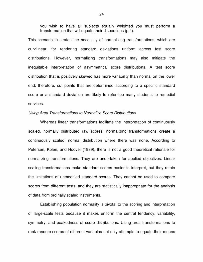
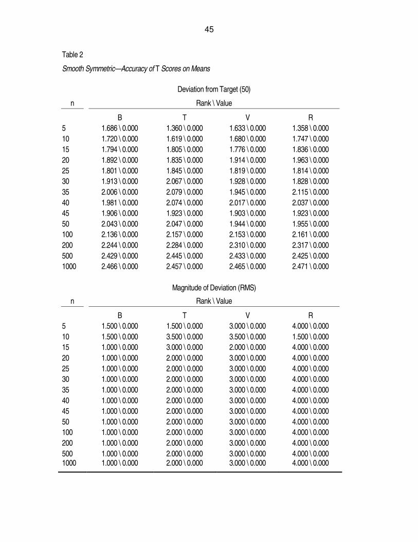
Psychometric distributions. Mass at Zero with Gap, Extreme Asymmetric,

Decay, and Extreme Bimodal were drawn from psychometric measures. These

distributions are illustrated in Figures 10 through 12.

All eight achievement and psychometric distributions are nonnormal.

Presentation of Results

Tables will document each ranking method’s performance in terms of

attaining the T score’s specified mean (50) and standard deviation (10), and the

skewness (0) and kurtosis (3) of the unit normal distribution.

35

Score

2520151050

Fre

qu

en

cy

500

400

300

200

100

0

Figure 5. Achievement: Smooth Symmetric. (Sawilowsky & Fahoome, 2003)

Basic characteristics of this distribution:

Range: (0 ≤ x ≤ 27)

Mean: 13.19

Median: 13.00

Variance: 24.11

Skewness: 0.01

Kurtosis: 2.66

36

Score

2520151050

Fre

qu

en

cy

300

250

200

150

100

50

0

Figure 6. Achievement: Discrete Mass at Zero. (Sawilowsky & Fahoome,

2003)


Range: (0 ≤ x ≤ 27)

Mean: 12.92

Median: 13.00

Variance: 19.54

Skewness: -0.03

Kurtosis: 3.31

37

Score

30252015105

Fre

qu

en

cy

500

400

300

200

100

0

Figure 7. Achievement: Extreme Asymmetric – Growth. (Sawilowsky &

Fahoome, 2003)


Range: (4 ≤ x ≤ 30)

Mean: 24.50

Median: 27.00

Variance: 33.52

Skewness: -1.33

Kurtosis: 4.11

38

Score

620595570545520495470445420

Fre

qu

en

cy

300

250

200

150

100

50

0

Figure 8. Achievement: Digit Preference. (Sawilowsky & Fahoome, 2003)


Range: (420 ≤ x ≤ 635)

Mean: 536.95

Median: 535.00

Variance: 1416.77

Skewness: -0.07

Kurtosis: 2.76

39

Score

4035302520151050

Fre

qu

en

cy

25

20

15

10

5

0

Figure 9. Achievement: Multimodal Lumpy. (Sawilowsky & Fahoome, 2003)


Range: (0 ≤ x ≤ 43)

Mean: 21.15

Median: 18.00

Variance: 141.61

Skewness: 0.19

Kurtosis: 1.80

40

Score

151050

Fre

qu

en

cy

600

500

400

300

200

100

0

Figure 10. Psychometric: Mass at Zero with Gap. (Sawilowsky & Fahoome,

2003)


Range: (0 ≤ x ≤ 16)

Mean: 1.85

Median: 0

Variance: 14.44

Skewness: 1.65

Kurtosis: 3.98

41

Score

3025201510

Fre

qu

en

cy

1200

1000

800

600

400

200

0

Figure 11. Psychometric: Extreme Asymmetric – Decay. (Sawilowsky &

Fahoome, 2003)


Range: (10 ≤ x ≤ 30)

Mean: 13.67

Median: 11.00

Variance: 33.06

Skewness: 1.64

Kurtosis: 4.52

42

Score

543210

Fre

qu

en

cy

250

200

150

100

50

0

Figure 12. Psychometric: Extreme Bimodal. (Sawilowsky & Fahoome, 2003)


Range: (0 ≤ x ≤ 5)

Mean: 2.97

Median: 4.00

Variance: 2.86

Skewness: -0.80

Kurtosis: 1.30

43

CHAPTER 4

RESULTS

The purpose of this study was to compare the accuracy of the Blom, Tukey,

Van der Waerden, and Rankit approximations. The following 32 tables present the

results. They show the absolute and relative accuracy of the four approximations in

attaining the target moments of the normal distribution at the values established by

the T score scale. The tables are organized sequentially according to distribution

and moment. Study results for the mean, the standard deviation, skewness, and

kurtosis appear in the same order for each of the eight distributions described in

Chapter 3. All numbers are rounded to the third decimal place.

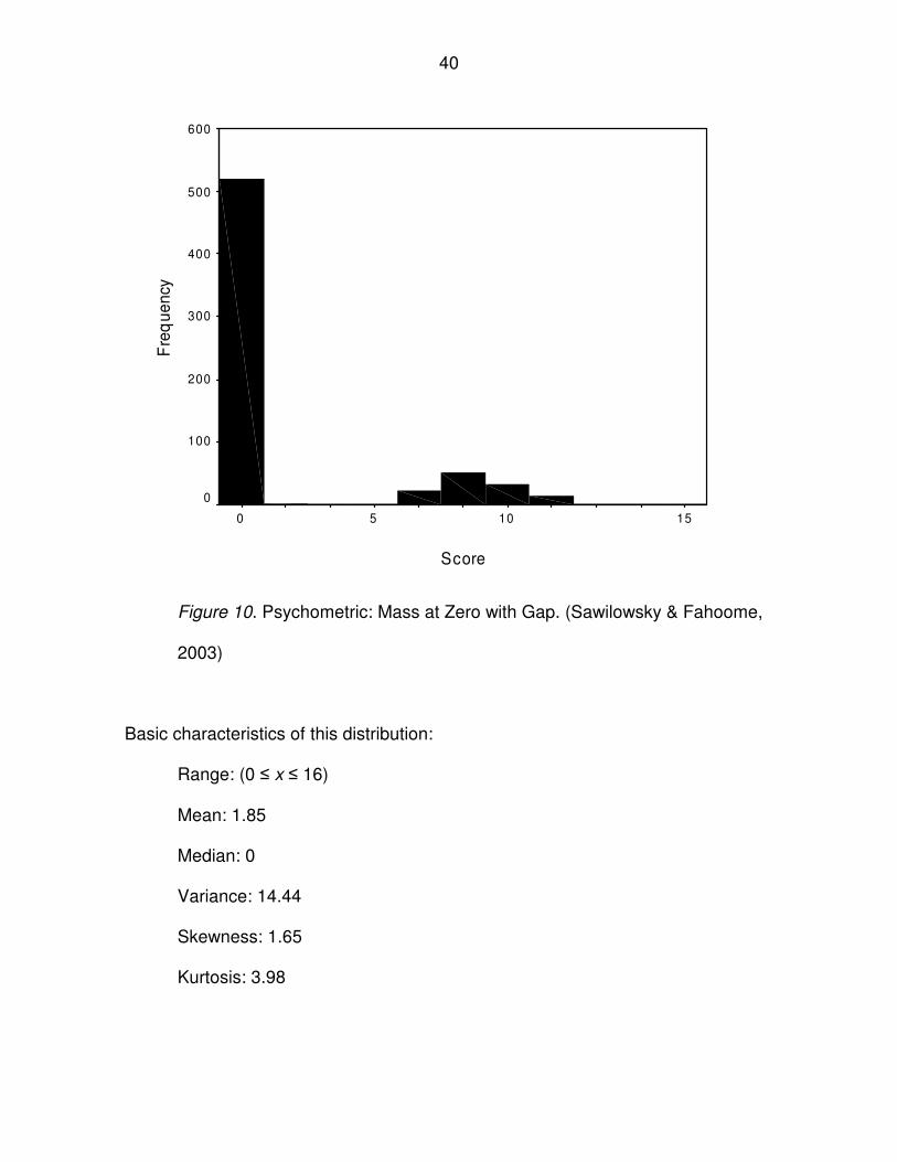
The accuracy of the four ranking methods on the T score is given in two

forms. The first, which comes to the left of the backslash ( \ ), represents the

statistic’s rank relative to the other three approximations. The number to the right

of the backslash represents an actual value, not a rank. The top half of each table

displays the relative ranks and absolute values of approximated scores’ deviation

from the target value of the given moment. For example, the T score’s target

standard deviation is 10. Therefore, the deviation value represents the absolute

value of the distance of each approximation from 10. Two ranking methods that

produce a standard deviation of 9.8 or 10.2 would have the same the deviation

value: 0.2. The bottom half of the tables displays the ranks and values of the root

mean square (RMS). RMS values, which represent the magnitude of difference

between scores, are derived by taking the standard deviations of each set of

mean, standard deviation, skewness, and kurtosis values. Both deviation from

44

target (the top half of the tables) and RMS (the bottom half) compare the four

approximations’ variability. Whereas deviation from target computes each ranking

method’s hit rate, or how frequently it is accurate, RMS evaluates the degree of

difference between the methods’ performance. It is possible for an approximation

to have different ranks in terms of deviation from target and magnitude of

deviation.

The rank, which is the first number in each column, is a whole number when

the approximation method achieves the same rank over 10,000 Monte Carlo runs.

It is a decimal when this is not the case. However, unlike deviation ranks, RMS

ranks correspond to a single statistic: the standard deviation of the respective

statistic’s average performance across 10,000 random draws. Therefore, ties are

possible between RMS ranks. There are 18 instances of tied RMS ranks

distributed among nine tables. Ties are broken by assigning to each tied rank the

average value of the tied ranks and the missing rank. For example, the two-way tie

(1, 1, 3, 4) is missing the rank of (2). The first two ranks are reassigned as the

mean of (1) and (2): (1.5, 1.5, 3, 4). Three-way ties, which are rare, are broken in

the same way: (1, 1, 1, 4) becomes (2, 2, 2, 4), representing the midpoint of (1)

and the missing ranks of (2) and (3).

The final statistic that is provided in the tables is the range for deviation from

target and RMS. In both cases, the range represents the difference between the

highest and the lowest values (not the ranks) in each row. The larger the range,

the more the deviation and RMS ranks are likely to matter. Following the 32 tables

documenting accuracy, a series of figures explores the deviation range.

45

Table 2

Smooth Symmetric—Accuracy of T Scores on Means

Deviation from Target (50)

n Rank \ Value

B T V R

5 1.686 \ 0.000 1.360 \ 0.000 1.633 \ 0.000 1.358 \ 0.000

10 1.720 \ 0.000 1.619 \ 0.000 1.680 \ 0.000 1.747 \ 0.000

15 1.794 \ 0.000 1.805 \ 0.000 1.776 \ 0.000 1.836 \ 0.000

20 1.892 \ 0.000 1.835 \ 0.000 1.914 \ 0.000 1.963 \ 0.000

25 1.801 \ 0.000 1.845 \ 0.000 1.819 \ 0.000 1.814 \ 0.000

30 1.913 \ 0.000 2.067 \ 0.000 1.928 \ 0.000 1.828 \ 0.000

35 2.006 \ 0.000 2.079 \ 0.000 1.945 \ 0.000 2.115 \ 0.000

40 1.981 \ 0.000 2.074 \ 0.000 2.017 \ 0.000 2.037 \ 0.000

45 1.906 \ 0.000 1.923 \ 0.000 1.903 \ 0.000 1.923 \ 0.000

50 2.043 \ 0.000 2.047 \ 0.000 1.944 \ 0.000 1.955 \ 0.000

100 2.136 \ 0.000 2.157 \ 0.000 2.153 \ 0.000 2.161 \ 0.000

200 2.244 \ 0.000 2.284 \ 0.000 2.310 \ 0.000 2.317 \ 0.000

500 2.429 \ 0.000 2.445 \ 0.000 2.433 \ 0.000 2.425 \ 0.000

1000 2.466 \ 0.000 2.457 \ 0.000 2.465 \ 0.000 2.471 \ 0.000

Magnitude of Deviation (RMS)

n Rank \ Value

B T V R

5 1.500 \ 0.000 1.500 \ 0.000 3.000 \ 0.000 4.000 \ 0.000

10 1.500 \ 0.000 3.500 \ 0.000 3.500 \ 0.000 1.500 \ 0.000

15 1.000 \ 0.000 3.000 \ 0.000 2.000 \ 0.000 4.000 \ 0.000

20 1.000 \ 0.000 2.000 \ 0.000 3.000 \ 0.000 4.000 \ 0.000

25 1.000 \ 0.000 2.000 \ 0.000 3.000 \ 0.000 4.000 \ 0.000

30 1.000 \ 0.000 2.000 \ 0.000 3.000 \ 0.000 4.000 \ 0.000

35 1.000 \ 0.000 2.000 \ 0.000 3.000 \ 0.000 4.000 \ 0.000

40 1.000 \ 0.000 2.000 \ 0.000 3.000 \ 0.000 4.000 \ 0.000

45 1.000 \ 0.000 2.000 \ 0.000 3.000 \ 0.000 4.000 \ 0.000

50 1.000 \ 0.000 2.000 \ 0.000 3.000 \ 0.000 4.000 \ 0.000

100 1.000 \ 0.000 2.000 \ 0.000 3.000 \ 0.000 4.000 \ 0.000

200 1.000 \ 0.000 2.000 \ 0.000 3.000 \ 0.000 4.000 \ 0.000

500 1.000 \ 0.000 2.000 \ 0.000 3.000 \ 0.000 4.000 \ 0.000 1000 1.000 \ 0.000 2.000 \ 0.000 3.000 \ 0.000 4.000 \ 0.000

46

Table 3

Smooth Symmetric—Accuracy of T Scores on Standard Deviations


n Rank \ Value Range

B T V R

5 1.000 \ 1.987 3.000 \ 2.177 4.000 \ 3.372 2.000 \ 2.089 1.385

10 1.000 \ 1.161 3.000 \ 1.296 4.000 \ 2.185 2.000 \ 1.185 1.024

15 1.998 \ 0.844 3.000 \ 0.951 4.000 \ 1.667 1.002 \ 0.842 0.825

20 2.000 \ 0.671 3.000 \ 0.760 4.000 \ 1.367 1.000 \ 0.659 0.708

25 2.000 \ 0.561 3.000 \ 0.638 4.000 \ 1.168 1.000 \ 0.544 0.624

30 2.000 \ 0.485 3.000 \ 0.554 4.000 \ 1.026 1.000 \ 0.465 0.561

35 2.000 \ 0.429 3.000 \ 0.491 4.000 \ 0.918 1.000 \ 0.408 0.510

40 2.000 \ 0.386 3.000 \ 0.442 4.000 \ 0.833 1.000 \ 0.364 0.469

45 2.000 \ 0.351 3.000 \ 0.403 4.000 \ 0.764 1.000 \ 0.329 0.435

50 2.000 \ 0.323 3.000 \ 0.371 4.000 \ 0.707 1.000 \ 0.300 0.407

100 2.000 \ 0.186 3.000 \ 0.215 4.000 \ 0.421 1.000 \ 0.167 0.254

200 2.000 \ 0.111 3.000 \ 0.128 4.000 \ 0.250 1.000 \ 0.010 0.240

500 2.000 \ 0.006 3.000 \ 0.007 4.000 \ 0.128 1.000 \ 0.005 0.123

1000 2.000 \ 0.004 3.000 \ 0.005 4.000 \ 0.008 1.000 \ 0.004 0.004



B T V R

5 3.000 \ 0.008 4.000 \ 0.008 2.000 \ 0.007 1.000 \ 0.007 0.001

10 3.000 \ 0.005 4.000 \ 0.005 2.000 \ 0.005 1.000 \ 0.004 0.001

15 3.000 \ 0.004 4.000 \ 0.004 2.000 \ 0.004 1.000 \ 0.003 0.001

20 3.000 \ 0.004 4.000 \ 0.004 2.000 \ 0.004 1.000 \ 0.003 0.001

25 3.000 \ 0.003 4.000 \ 0.003 2.000 \ 0.003 1.000 \ 0.002 0.001

30 4.000 \ 0.003 3.000 \ 0.003 2.000 \ 0.003 1.000 \ 0.002 0.001

35 3.000 \ 0.002 4.000 \ 0.002 2.000 \ 0.002 1.000 \ 0.001 0.001

40 3.000 \ 0.002 4.000 \ 0.002 2.000 \ 0.002 1.000 \ 0.001 0.001

45 4.000 \ 0.001 3.000 \ 0.001 2.000 \ 0.001 1.000 \ 0.001 0.000

50 3.000 \ 0.001 4.000 \ 0.001 2.000 \ 0.001 1.000 \ 0.001 0.000

100 4.000 \ 0.001 3.000 \ 0.001 2.000 \ 0.001 1.000 \ 0.000 0.001

200 4.000 \ 0.000 3.000 \ 0.000 2.000 \ 0.000 1.000 \ 0.000 0.000

500 4.000 \ 0.000 3.000 \ 0.000 2.000 \ 0.000 1.000 \ 0.000 0.000 1000 4.000 \ 0.000 3.000 \ 0.000 2.000 \ 0.000 1.000 \ 0.000 0.000

47

Table 4

Smooth Symmetric—Accuracy of T Scores on Skewness



B T V R

5 3.717 \ 0.000 2.895 \ 0.000 1.295 \ 0.000 2.093 \ 0.000 0.000

10 3.936 \ 0.001 1.914 \ 0.000 1.232 \ 0.001 2.919 \ 0.001 0.001

15 1.013 \ 0.001 2.994 \ 0.001 3.989 \ 0.105 2.004 \ 0.001 0.104

20 2.006 \ 0.140 2.997 \ 0.140 3.987 \ 0.146 1.010 \ 0.140 0.006

25 1.995 \ 0.122 3.000 \ 0.122 4.000 \ 0.127 1.007 \ 0.122 0.005

30 2.000 \ 0.007 3.000 \ 0.007 4.000 \ 0.007 1.000 \ 0.007 0.000

35 1.993 \ 0.001 2.997 \ 0.001 3.994 \ 0.001 1.016 \ 0.001 0.000

40 2.116 \ 0.000 2.908 \ 0.000 3.732 \ 0.000 1.244 \ 0.000 0.000

45 2.007 \ 0.001 3.000 \ 0.001 3.989 \ 0.001 1.008 \ 0.001 0.000

50 2.020 \ 0.141 2.989 \ 0.141 3.965 \ 0.145 1.027 \ 0.141 0.004

100 2.937 \ 0.002 2.055 \ 0.002 1.170 \ 0.002 3.838 \ 0.002 0.000

200 2.930 \ 0.003 2.063 \ 0.003 1.190 \ 0.003 3.817 \ 0.003 0.000

500 2.897 \ 0.003 2.082 \ 0.003 1.233 \ 0.003 3.788 \ 0.003 0.000

1000 2.875 \ 0.003 2.094 \ 0.003 1.288 \ 0.003 3.743 \ 0.003 0.000



B T V R

5 1.000 \ 0.002 2.000 \ 0.002 4.000 \ 0.002 3.000 \ 0.002 0.000

10 1.000 \ 0.256 3.000 \ 0.259 4.000 \ 0.279 2.000 \ 0.258 0.023

15 4.000 \ 0.521 2.000 \ 0.520 1.000 \ 0.515 3.000 \ 0.520 0.006

20 1.000 \ 0.446 3.000 \ 0.447 4.000 \ 0.456 2.000 \ 0.446 0.010

25 4.000 \ 0.570 2.000 \ 0.567 1.000 \ 0.551 3.000 \ 0.570 0.019

30 4.000 \ 0.453 2.000 \ 0.450 1.000 \ 0.436 3.000 \ 0.452 0.017

35 3.000 \ 0.479 2.000 \ 0.477 1.000 \ 0.461 4.000 \ 0.479 0.018

40 3.000 \ 0.612 2.000 \ 0.611 1.000 \ 0.560 4.000 \ 0.613 0.053

45 3.000 \ 0.587 2.000 \ 0.586 1.000 \ 0.578 4.000 \ 0.587 0.009

50 3.000 \ 0.607 2.000 \ 0.605 1.000 \ 0.593 4.000 \ 0.608 0.015

100 3.000 \ 0.565 2.000 \ 0.565 1.000 \ 0.564 4.000 \ 0.565 0.001

200 3.000 \ 0.555 2.000 \ 0.555 4.000 \ 0.555 1.000 \ 0.555 0.000

500 3.000 \ 0.549 2.000 \ 0.549 4.000 \ 0.549 1.000 \ 0.549 0.000 1000 3.000 \ 0.555 2.000 \ 0.555 1.000 \ 0.555 4.000 \ 0.555 0.000

48

Table 5

Smooth Symmetric—Accuracy of T Scores on Kurtosis



B T V R

5 1.000 \ 1.148 2.000 \ 1.155 4.000 \ 1.195 3.000 \ 1.156 0.047

10 1.000 \ 1.106 3.000 \ 1.111 4.000 \ 1.138 2.000 \ 1.110 0.032

15 1.000 \ 1.092 3.000 \ 1.095 4.000 \ 1.115 2.000 \ 1.093 0.023

20 1.001 \ 1.058 3.000 \ 1.061 4.000 \ 1.079 2.002 \ 1.058 0.021

25 1.922 \ 1.019 3.000 \ 1.022 4.000 \ 1.040 1.078 \ 1.019 0.021

30 2.000 \ 0.981 3.000 \ 0.983 4.000 \ 1.000 1.000 \ 0.980 0.020

35 2.000 \ 0.957 3.000 \ 0.959 4.000 \ 0.975 1.000 \ 0.956 0.019

40 2.000 \ 0.953 3.000 \ 0.956 4.000 \ 0.970 1.000 \ 0.953 0.017

45 2.000 \ 0.979 3.000 \ 0.980 4.000 \ 0.993 1.000 \ 0.978 0.015

50 2.000 \ 1.014 3.000 \ 1.016 4.000 \ 1.028 1.000 \ 1.013 0.015

100 2.000 \ 0.957 3.000 \ 0.960 4.000 \ 0.976 1.000 \ 0.956 0.020

200 2.000 \ 0.948 3.000 \ 0.950 4.000 \ 0.961 1.000 \ 0.947 0.014

500 2.000 \ 0.942 3.000 \ 0.943 4.000 \ 0.949 1.000 \ 0.941 0.008

1000 2.000 \ 0.940 3.000 \ 0.940 4.000 \ 0.944 1.000 \ 0.939 0.005



B T V R

5 1.000 \ 0.006 2.000 \ 0.006 4.000 \ 0.006 3.000 \ 0.006 0.000

10 2.000 \ 0.310 3.000 \ 0.311 4.000 \ 0.313 1.000 \ 0.310 0.003

15 1.000 \ 0.434 3.000 \ 0.435 4.000 \ 0.438 2.000 \ 0.435 0.004

20 1.000 \ 0.402 3.000 \ 0.403 4.000 \ 0.411 2.000 \ 0.402 0.009

25 4.000 \ 0.470 2.000 \ 0.469 1.000 \ 0.462 3.000 \ 0.470 0.008

30 4.000 \ 0.456 2.000 \ 0.456 1.000 \ 0.452 3.000 \ 0.456 0.004

35 3.000 \ 0.444 2.000 \ 0.444 1.000 \ 0.443 4.000 \ 0.444 0.001

40 3.000 \ 0.462 2.000 \ 0.461 1.000 \ 0.457 4.000 \ 0.462 0.005

45 3.000 \ 0.500 2.000 \ 0.500 1.000 \ 0.498 4.000 \ 0.500 0.002

50 3.000 \ 0.495 2.000 \ 0.495 1.000 \ 0.494 4.000 \ 0.495 0.001

100 2.000 \ 0.476 3.000 \ 0.476 4.000 \ 0.476 1.000 \ 0.476 0.000

200 2.000 \ 0.477 3.000 \ 0.477 4.000 \ 0.478 1.000 \ 0.477 0.001

500 2.000 \ 0.472 3.000 \ 0.472 4.000 \ 0.472 1.000 \ 0.472 0.000 1000 2.000 \ 0.472 3.000 \ 0.472 4.000 \ 0.473 1.000 \ 0.472 0.001

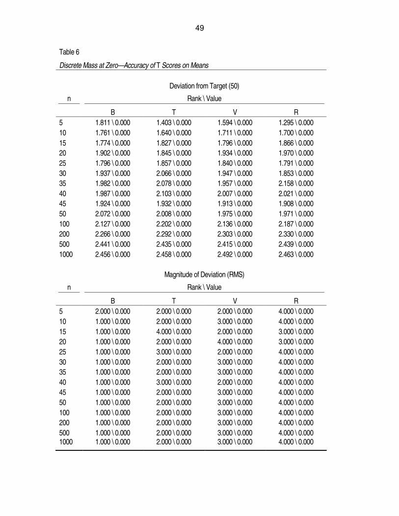
49

Table 6

Discrete Mass at Zero—Accuracy of T Scores on Means


n Rank \ Value

B T V R

5 1.811 \ 0.000 1.403 \ 0.000 1.594 \ 0.000 1.295 \ 0.000

10 1.761 \ 0.000 1.640 \ 0.000 1.711 \ 0.000 1.700 \ 0.000

15 1.774 \ 0.000 1.827 \ 0.000 1.796 \ 0.000 1.866 \ 0.000

20 1.902 \ 0.000 1.845 \ 0.000 1.934 \ 0.000 1.970 \ 0.000

25 1.796 \ 0.000 1.857 \ 0.000 1.840 \ 0.000 1.791 \ 0.000

30 1.937 \ 0.000 2.066 \ 0.000 1.947 \ 0.000 1.853 \ 0.000

35 1.982 \ 0.000 2.078 \ 0.000 1.957 \ 0.000 2.158 \ 0.000

40 1.987 \ 0.000 2.103 \ 0.000 2.007 \ 0.000 2.021 \ 0.000

45 1.924 \ 0.000 1.932 \ 0.000 1.913 \ 0.000 1.908 \ 0.000

50 2.072 \ 0.000 2.008 \ 0.000 1.975 \ 0.000 1.971 \ 0.000

100 2.127 \ 0.000 2.202 \ 0.000 2.136 \ 0.000 2.187 \ 0.000

200 2.266 \ 0.000 2.292 \ 0.000 2.303 \ 0.000 2.330 \ 0.000

500 2.441 \ 0.000 2.435 \ 0.000 2.415 \ 0.000 2.439 \ 0.000

1000 2.456 \ 0.000 2.458 \ 0.000 2.492 \ 0.000 2.463 \ 0.000


n Rank \ Value

B T V R

5 2.000 \ 0.000 2.000 \ 0.000 2.000 \ 0.000 4.000 \ 0.000

10 1.000 \ 0.000 2.000 \ 0.000 3.000 \ 0.000 4.000 \ 0.000

15 1.000 \ 0.000 4.000 \ 0.000 2.000 \ 0.000 3.000 \ 0.000

20 1.000 \ 0.000 2.000 \ 0.000 4.000 \ 0.000 3.000 \ 0.000

25 1.000 \ 0.000 3.000 \ 0.000 2.000 \ 0.000 4.000 \ 0.000

30 1.000 \ 0.000 2.000 \ 0.000 3.000 \ 0.000 4.000 \ 0.000

35 1.000 \ 0.000 2.000 \ 0.000 3.000 \ 0.000 4.000 \ 0.000

40 1.000 \ 0.000 3.000 \ 0.000 2.000 \ 0.000 4.000 \ 0.000

45 1.000 \ 0.000 2.000 \ 0.000 3.000 \ 0.000 4.000 \ 0.000

50 1.000 \ 0.000 2.000 \ 0.000 3.000 \ 0.000 4.000 \ 0.000

100 1.000 \ 0.000 2.000 \ 0.000 3.000 \ 0.000 4.000 \ 0.000

200 1.000 \ 0.000 2.000 \ 0.000 3.000 \ 0.000 4.000 \ 0.000

500 1.000 \ 0.000 2.000 \ 0.000 3.000 \ 0.000 4.000 \ 0.000 1000 1.000 \ 0.000 2.000 \ 0.000 3.000 \ 0.000 4.000 \ 0.000

50

Table 7

Discrete Mass at Zero—Accuracy of T Scores on Standard Deviations



B T V R

5 1.000 \ 2.049 3.000 \ 2.237 4.000 \ 3.421 2.000 \ 2.149 1.372

10 1.000 \ 1.182 3.000 \ 1.316 4.000 \ 2.202 2.000 \ 1.205 1.020

15 1.997 \ 0.853 3.000 \ 0.959 4.000 \ 1.675 1.003 \ 0.851 0.824

20 2.000 \ 0.675 3.000 \ 0.764 4.000 \ 1.370 1.000 \ 0.663 0.707

25 2.000 \ 0.571 3.000 \ 0.648 4.000 \ 1.176 1.000 \ 0.553 0.623

30 2.000 \ 0.496 3.000 \ 0.564 4.000 \ 1.035 1.000 \ 0.476 0.559

35 2.000 \ 0.440 3.000 \ 0.501 4.000 \ 0.927 1.000 \ 0.418 0.509

40 2.000 \ 0.396 3.000 \ 0.452 4.000 \ 0.842 1.000 \ 0.374 0.468

45 3.000 \ 0.368 3.000 \ 0.412 4.000 \ 0.773 1.000 \ 0.338 0.435

50 2.000 \ 0.333 3.000 \ 0.381 4.000 \ 0.716 1.000 \ 0.310 0.406

100 2.000 \ 0.195 3.000 \ 0.224 4.000 \ 0.429 1.000 \ 0.176 0.253

200 2.000 \ 0.120 3.000 \ 0.137 4.000 \ 0.258 1.000 \ 0.106 0.152

500 2.000 \ 0.007 3.000 \ 0.008 4.000 \ 0.137 1.000 \ 0.006 0.131

1000 2.000 \ 0.005 3.000 \ 0.006 4.000 \ 0.009 1.000 \ 0.005 0.004



B T V R

5 4.000 \ 0.117 3.000 \ 0.114 2.000 \ 0.113 1.000 \ 0.009 0.108

10 4.000 \ 0.008 3.000 \ 0.008 2.000 \ 0.008 1.000 \ 0.006 0.002

15 3.000 \ 0.005 4.000 \ 0.005 2.000 \ 0.005 1.000 \ 0.004 0.001

20 3.000 \ 0.004 4.000 \ 0.004 2.000 \ 0.004 1.000 \ 0.003 0.001

25 3.000 \ 0.003 4.000 \ 0.003 2.000 \ 0.003 1.000 \ 0.002 0.001

30 4.000 \ 0.004 3.000 \ 0.004 2.000 \ 0.004 1.000 \ 0.003 0.001

35 4.000 \ 0.002 3.000 \ 0.002 2.000 \ 0.002 1.000 \ 0.002 0.000

40 3.000 \ 0.002 4.000 \ 0.002 2.000 \ 0.002 1.000 \ 0.001 0.001

45 4.000 \ 0.002 3.000 \ 0.002 2.000 \ 0.002 1.000 \ 0.001 0.001

50 4.000 \ 0.001 3.000 \ 0.001 2.000 \ 0.001 1.000 \ 0.001 0.000

100 4.000 \ 0.001 3.000 \ 0.001 2.000 \ 0.001 1.000 \ 0.001 0.000

200 4.000 \ 0.000 3.000 \ 0.000 2.000 \ 0.000 1.000 \ 0.000 0.000

500 4.000 \ 0.000 3.000 \ 0.000 2.000 \ 0.000 1.000 \ 0.000 0.000 1000 4.000 \ 0.000 3.000 \ 0.000 2.000 \ 0.000 1.000 \ 0.000 0.000

51

Table 8

Discrete Mass at Zero—Accuracy of T Scores on Skewness



B T V R

5 3.740 \ 0.001 2.914 \ 0.001 1.264 \ 0.001 2.083 \ 0.001 0.000

10 1.005 \ 0.004 2.999 \ 0.005 3.996 \ 0.006 2.001 \ 0.005 0.002

15 2.880 \ 0.006 2.302 \ 0.006 2.238 \ 0.004 2.579 \ 0.006 0.002

20 3.983 \ 0.007 2.007 \ 0.006 1.023 \ 0.005 2.987 \ 0.007 0.002

25 2.274 \ 0.003 2.382 \ 0.004 3.197 \ 0.005 2.147 \ 0.003 0.002

30 2.005 \ 0.127 2.994 \ 0.128 3.985 \ 0.134 1.015 \ 0.127 0.007

35 2.017 \ 0.139 2.989 \ 0.140 3.968 \ 0.145 1.026 \ 0.139 0.006

40 2.000 \ 0.119 3.000 \ 0.120 3.999 \ 0.123 1.001 \ 0.119 0.004

45 2.003 \ 0.007 2.997 \ 0.007 3.992 \ 0.007 1.008 \ 0.007 0.000

50 2.007 \ 0.002 2.999 \ 0.002 3.972 \ 0.002 1.023 \ 0.002 0.000

100 2.881 \ 0.001 2.074 \ 0.001 1.339 \ 0.000 3.706 \ 0.001 0.001

200 3.001 \ 0.003 2.019 \ 0.003 1.069 \ 0.003 3.912 \ 0.003 0.000

500 2.965 \ 0.003 2.026 \ 0.003 1.033 \ 0.003 3.975 \ 0.003 0.000

1000 2.863 \ 0.001 2.127 \ 0.001 1.403 \ 0.001 3.607 \ 0.001 0.000



B T V R

5 4.000 \ 0.010 3.000 \ 0.010 1.000 \ 0.009 2.000 \ 0.010 0.001

10 4.000 \ 0.469 2.000 \ 0.467 1.000 \ 0.459 3.000 \ 0.467 0.010

15 1.000 \ 0.313 3.000 \ 0.313 4.000 \ 0.320 2.000 \ 0.313 0.007

20 1.000 \ 0.473 3.000 \ 0.473 4.000 \ 0.479 2.000 \ 0.473 0.006

25 4.000 \ 0.382 2.000 \ 0.382 1.000 \ 0.382 3.000 \ 0.382 0.000

30 4.000 \ 0.526 2.000 \ 0.525 1.000 \ 0.524 3.000 \ 0.526 0.002

35 3.000 \ 0.535 2.000 \ 0.535 1.000 \ 0.520 4.000 \ 0.535 0.015

40 3.000 \ 0.608 2.000 \ 0.607 1.000 \ 0.598 4.000 \ 0.609 0.011

45 3.000 \ 0.535 2.000 \ 0.559 1.000 \ 0.551 4.000 \ 0.560 0.025

50 3.000 \ 0.566 2.000 \ 0.565 1.000 \ 0.558 4.000 \ 0.567 0.009

100 3.000 \ 0.559 2.000 \ 0.559 1.000 \ 0.558 4.000 \ 0.558 0.001

200 3.000 \ 0.555 2.000 \ 0.555 4.000 \ 0.555 1.000 \ 0.555 0.000

500 4.000 \ 0.552 2.000 \ 0.552 1.000 \ 0.552 3.000 \ 0.552 0.000 1000 2.000 \ 0.542 1.000 \ 0.542 4.000 \ 0.542 3.000 \ 0.542 0.000

52

Table 9

Discrete Mass at Zero—Accuracy of T Scores on Kurtosis



B T V R

5 1.000 \ 1.164 2.000 \ 1.171 4.000 \ 1.208 3.000 \ 1.172 0.044

10 1.000 \ 1.109 2.100 \ 1.114 3.100 \ 1.139 2.000 \ 1.112 0.030

15 1.001 \ 1.070 3.000 \ 1.074 3.999 \ 1.098 2.000 \ 1.072 0.028

20 1.000 \ 1.016 3.000 \ 1.020 4.000 \ 1.047 2.000 \ 1.017 0.031

25 1.001 \ 1.078 3.000 \ 1.081 4.000 \ 1.095 1.999 \ 1.078 0.017

30 2.000 \ 1.075 3.000 \ 1.077 4.000 \ 1.091 1.000 \ 1.075 0.016

35 2.000 \ 1.044 3.000 \ 1.046 4.000 \ 1.060 1.000 \ 1.043 0.017

40 2.000 \ 0.996 3.000 \ 0.999 3.999 \ 1.012 1.000 \ 0.996 0.016

45 2.000 \ 0.953 3.000 \ 0.955 4.000 \ 0.968 1.000 \ 0.953 0.015

50 2.000 \ 0.945 3.000 \ 0.946 4.000 \ 0.959 1.000 \ 0.944 0.015

100 2.000 \ 1.081 3.000 \ 1.082 3.999 \ 1.088 1.001 \ 1.080 0.008

200 2.000 \ 0.949 3.000 \ 0.950 4.000 \ 0.961 1.000 \ 0.947 0.014

500 2.000 \ 0.942 3.000 \ 0.943 4.000 \ 0.949 1.000 \ 0.941 0.008

1000 2.000 \ 1.081 3.000 \ 1.081 3.999 \ 1.082 1.001 \ 1.081 0.001



B T V R

5 4.000 \ 0.010 3.000 \ 0.010 1.000 \ 0.009 2.000 \ 0.010 0.001

10 1.000 \ 0.304 3.000 \ 0.306 4.000 \ 0.320 2.000 \ 0.305 0.016

15 1.000 \ 0.339 3.000 \ 0.340 4.000 \ 0.348 2.000 \ 0.339 0.009

20 1.000 \ 0.326 3.000 \ 0.327 4.000 \ 0.332 2.000 \ 0.326 0.006

25 1.000 \ 0.397 3.000 \ 0.397 4.000 \ 0.398 2.000 \ 0.397 0.001

30 2.000 \ 0.502 3.000 \ 0.502 4.000 \ 0.505 1.000 \ 0.502 0.003

35 4.000 \ 0.354 2.000 \ 0.354 1.000 \ 0.354 3.000 \ 0.354 0.000

40 2.000 \ 0.468 3.000 \ 0.468 4.000 \ 0.469 1.000 \ 0.468 0.001

45 3.000 \ 0.503 2.000 \ 0.503 1.000 \ 0.500 4.000 \ 0.503 0.003

50 3.000 \ 0.465 2.000 \ 0.465 1.000 \ 0.464 4.000 \ 0.466 0.002

100 2.000 \ 0.494 3.000 \ 0.494 4.000 \ 0.495 1.000 \ 0.494 0.001

200 2.000 \ 0.480 3.000 \ 0.480 4.000 \ 0.480 1.000 \ 0.480 0.000

500 2.000 \ 0.477 3.000 \ 0.477 4.000 \ 0.477 1.000 \ 0.477 0.000 1000 2.000 \ 0.473 3.000 \ 0.473 4.000 \ 0.473 1.000 \ 0.473 0.000

53

Table 10

Extreme Asymmetric, Growth—Accuracy of T Scores on Means


n Rank \ Value

B T V R

5 1.738 \ 0.000 1.411 \ 0.000 1.579 \ 0.000 1.196 \ 0.000

10 1.796 \ 0.000 1.669 \ 0.000 1.837 \ 0.000 1.630 \ 0.000

15 1.827 \ 0.000 1.810 \ 0.000 1.846 \ 0.000 1.778 \ 0.000

20 2.039 \ 0.000 1.878 \ 0.000 1.936 \ 0.000 1.923 \ 0.000

25 1.822 \ 0.000 1.853 \ 0.000 1.825 \ 0.000 1.880 \ 0.000

30 1.977 \ 0.000 2.051 \ 0.000 2.004 \ 0.000 1.882 \ 0.000

35 2.076 \ 0.000 2.076 \ 0.000 2.049 \ 0.000 2.028 \ 0.000

40 2.091 \ 0.000 2.033 \ 0.000 2.041 \ 0.000 1.988 \ 0.000

45 1.943 \ 0.000 1.958 \ 0.000 1.881 \ 0.000 1.926 \ 0.000

50 2.043 \ 0.000 2.025 \ 0.000 1.967 \ 0.000 1.988 \ 0.000

100 2.143 \ 0.000 2.235 \ 0.000 2.192 \ 0.000 2.141 \ 0.000

200 2.276 \ 0.000 2.310 \ 0.000 2.314 \ 0.000 2.390 \ 0.000

500 2.411 \ 0.000 2.449 \ 0.000 2.474 \ 0.000 2.437 \ 0.000

1000 2.477 \ 0.000 2.474 \ 0.000 2.457 \ 0.000 2.477 \ 0.000


n Rank \ Value

B T V R

5 1.500 \ 0.000 1.500 \ 0.000 3.500 \ 0.000 3.500 \ 0.000

10 1.000 \ 0.000 2.000 \ 0.000 3.500 \ 0.000 3.500 \ 0.000

15 1.000 \ 0.000 4.000 \ 0.000 3.000 \ 0.000 2.000 \ 0.000

20 1.000 \ 0.000 4.000 \ 0.000 3.000 \ 0.000 2.000 \ 0.000

25 1.000 \ 0.000 2.000 \ 0.000 3.000 \ 0.000 4.000 \ 0.000

30 1.000 \ 0.000 2.000 \ 0.000 3.000 \ 0.000 4.000 \ 0.000

35 1.000 \ 0.000 2.000 \ 0.000 3.000 \ 0.000 4.000 \ 0.000

40 4.000 \ 0.000 1.000 \ 0.000 3.000 \ 0.000 2.000 \ 0.000

45 1.000 \ 0.000 2.000 \ 0.000 3.000 \ 0.000 4.000 \ 0.000

50 1.000 \ 0.000 2.000 \ 0.000 3.000 \ 0.000 4.000 \ 0.000

100 1.000 \ 0.000 2.000 \ 0.000 3.000 \ 0.000 4.000 \ 0.000

200 1.000 \ 0.000 2.000 \ 0.000 3.000 \ 0.000 4.000 \ 0.000

500 1.000 \ 0.000 2.000 \ 0.000 3.000 \ 0.000 4.000 \ 0.000 1000 1.000 \ 0.000 2.000 \ 0.000 3.000 \ 0.000 4.000 \ 0.000

54

Table 11

Extreme Asymmetric, Growth—Accuracy of T Scores on Standard Deviations



B T V R

5 1.000 \ 2.075 3.000 \ 2.263 4.000 \ 3.442 2.000 \ 2.176 1.367

10 1.000 \ 1.243 3.000 \ 1.375 4.000 \ 2.250 2.000 \ 1.265 1.007

15 1.984 \ 0.934 3.000 \ 1.038 4.000 \ 1.739 1.016 \ 0.932 0.807

20 2.000 \ 0.769 3.000 \ 0.855 4.000 \ 1.446 1.000 \ 0.756 0.690

25 2.000 \ 0.666 3.000 \ 0.740 4.000 \ 1.253 1.000 \ 0.649 0.604

30 2.000 \ 0.601 3.000 \ 0.666 4.000 \ 1.120 1.000 \ 0.581 0.539

35 2.000 \ 0.551 3.000 \ 0.609 4.000 \ 1.018 1.000 \ 0.530 0.488

40 2.000 \ 0.524 3.000 \ 0.577 4.000 \ 0.947 1.000 \ 0.502 0.445

45 2.000 \ 0.484 3.000 \ 0.532 4.000 \ 0.874 1.000 \ 0.462 0.412

50 2.000 \ 0.440 3.000 \ 0.485 4.000 \ 0.804 1.000 \ 0.418 0.386

100 2.000 \ 0.320 3.000 \ 0.347 4.000 \ 0.538 1.000 \ 0.302 0.236

200 2.000 \ 0.258 3.000 \ 0.273 4.000 \ 0.384 1.000 \ 0.245 0.139

500 2.000 \ 0.213 3.000 \ 0.220 4.000 \ 0.273 1.000 \ 0.205 0.068

1000 2.000 \ 0.197 3.000 \ 0.201 4.000 \ 0.230 1.000 \ 0.194 0.036



B T V R

5 4.000 \ 0.204 3.000 \ 0.200 2.000 \ 0.198 1.000 \ 0.163 0.041

10 4.000 \ 0.169 3.000 \ 0.168 2.000 \ 0.165 1.000 \ 0.144 0.025

15 3.000 \ 0.007 4.000 \ 0.007 2.000 \ 0.007 1.000 \ 0.006 0.001

20 3.000 \ 0.005 4.000 \ 0.005 2.000 \ 0.005 1.000 \ 0.004 0.001

25 4.000 \ 0.010 3.000 \ 0.010 2.000 \ 0.010 1.000 \ 0.008 0.002

30 4.000 \ 0.009 3.000 \ 0.009 2.000 \ 0.009 1.000 \ 0.008 0.001

35 4.000 \ 0.006 3.000 \ 0.006 2.000 \ 0.006 1.000 \ 0.005 0.001

40 4.000 \ 0.005 3.000 \ 0.005 2.000 \ 0.005 1.000 \ 0.005 0.000

45 4.000 \ 0.007 3.000 \ 0.007 2.000 \ 0.007 1.000 \ 0.006 0.001

50 4.000 \ 0.005 3.000 \ 0.005 2.000 \ 0.005 1.000 \ 0.005 0.000

100 4.000 \ 0.004 3.000 \ 0.004 2.000 \ 0.004 1.000 \ 0.004 0.000

200 4.000 \ 0.003 3.000 \ 0.003 2.000 \ 0.003 1.000 \ 0.003 0.000

500 4.000 \ 0.002 3.000 \ 0.002 2.000 \ 0.002 1.000 \ 0.002 0.000

1000 3.000 \ 0.001 4.000 \ 0.001 2.000 \ 0.001 1.000 \ 0.001 0.000

55

Table 12

Extreme Asymmetric, Growth—Accuracy of T Scores on Skewness



B T V R

5 4.000 \ 0.005 3.000 \ 0.005 1.000 \ 0.005 2.000 \ 0.005 0.000

10 1.076 \ 0.001 2.973 \ 0.001 3.928 \ 0.001 2.024 \ 0.001 0.000

15 3.424 \ 0.004 2.163 \ 0.004 1.624 \ 0.004 2.790 \ 0.004 0.000

20 1.582 \ 0.107 2.997 \ 0.107 3.988 \ 0.109 1.433 \ 0.107 0.002

25 1.998 \ 0.139 2.998 \ 0.139 3.994 \ 0.143 1.010 \ 0.139 0.004

30 2.000 \ 0.176 2.998 \ 0.177 3.994 \ 0.182 1.008 \ 0.176 0.006

35 2.004 \ 0.142 3.000 \ 0.142 3.992 \ 0.148 1.007 \ 0.141 0.007

40 2.000 \ 0.002 2.999 \ 0.002 3.998 \ 0.003 1.003 \ 0.002 0.001

45 2.149 \ 0.009 2.968 \ 0.009 3.798 \ 0.009 1.085 \ 0.009 0.000

50 3.000 \ 0.010 2.000 \ 0.010 1.000 \ 0.008 4.000 \ 0.010 0.002

100 2.006 \ 0.166 2.996 \ 0.167 3.990 \ 0.168 1.008 \ 0.166 0.002

200 2.591 \ 0.170 2.420 \ 0.169 2.316 \ 0.164 2.677 \ 0.171 0.007

500 2.615 \ 0.174 2.388 \ 0.174 2.193 \ 0.171 2.804 \ 0.175 0.004

1000 2.620 \ 0.176 2.379 \ 0.175 2.160 \ 0.174 2.841 \ 0.176 0.002



B T V R

5 4.000 \ 0.113 3.000 \ 0.111 1.000 \ 0.010 2.000 \ 0.110 0.103

10 3.000 \ 0.413 2.000 \ 0.412 1.000 \ 0.410 4.000 \ 0.413 0.003

15 4.000 \ 0.481 2.000 \ 0.478 1.000 \ 0.457 3.000 \ 0.480 0.024

20 4.000 \ 0.654 2.000 \ 0.652 1.000 \ 0.640 3.000 \ 0.654 0.014

25 3.000 \ 0.600 2.000 \ 0.597 1.000 \ 0.580 4.000 \ 0.600 0.020

30 4.000 \ 0.504 2.000 \ 0.503 1.000 \ 0.498 3.000 \ 0.504 0.006

35 3.000 \ 0.668 2.000 \ 0.668 1.000 \ 0.665 4.000 \ 0.669 0.004

40 3.000 \ 0.649 2.000 \ 0.648 1.000 \ 0.644 4.000 \ 0.649 0.005

45 3.000 \ 0.666 2.000 \ 0.665 1.000 \ 0.663 4.000 \ 0.666 0.003

50 2.000 \ 0.500 3.000 \ 0.500 4.000 \ 0.505 1.000 \ 0.500 0.005

100 3.000 \ 0.541 2.000 \ 0.540 1.000 \ 0.538 4.000 \ 0.541 0.003

200 3.000 \ 0.596 2.000 \ 0.596 1.000 \ 0.595 4.000 \ 0.596 0.001

500 3.000 \ 0.576 2.000 \ 0.576 1.000 \ 0.576 4.000 \ 0.576 0.000 1000 3.000 \ 0.590 2.000 \ 0.590 1.000 \ 0.590 4.000 \ 0.590 0.000

56

Table 13

Extreme Asymmetric, Growth—Accuracy of T Scores on Kurtosis



B T V R

5 1.000 \ 1.176 2.000 \ 1.182 4.000 \ 1.219 3.000 \ 1.183 0.043

10 1.000 \ 1.063 3.000 \ 1.064 4.000 \ 1.093 2.000 \ 1.066 0.030

15 1.000 \ 1.018 3.000 \ 1.022 4.000 \ 1.042 2.000 \ 1.019 0.024

20 1.000 \ 1.008 3.000 \ 1.010 4.000 \ 1.028 2.000 \ 1.008 0.020

25 2.000 \ 1.025 3.000 \ 1.027 4.000 \ 1.041 1.000 \ 1.025 0.016

30 2.000 \ 1.078 3.000 \ 1.079 4.000 \ 1.091 1.000 \ 1.077 0.014

35 2.000 \ 1.085 3.000 \ 1.087 4.000 \ 1.098 1.000 \ 1.085 0.013

40 2.000 \ 1.116 3.000 \ 1.117 4.000 \ 1.124 1.000 \ 1.115 0.009

45 2.000 \ 1.066 3.000 \ 1.067 4.000 \ 1.079 1.000 \ 1.065 0.014

50 2.000 \ 1.082 3.000 \ 1.083 4.000 \ 1.094 1.000 \ 1.081 0.013

100 2.001 \ 1.044 2.999 \ 1.045 3.998 \ 1.051 1.001 \ 1.043 0.008

200 2.001 \ 1.023 3.000 \ 1.024 3.999 \ 1.030 1.002 \ 1.022 0.008

500 2.001 \ 1.019 3.000 \ 1.020 3.999 \ 1.023 1.002 \ 1.019 0.004

1000 2.001 \ 1.018 3.000 \ 1.018 3.999 \ 1.020 1.002 \ 1.018 0.002



B T V R

5 4.000 \ 0.010 3.000 \ 0.009 1.000 \ 0.008 2.000 \ 0.009 0.002

10 1.000 \ 0.254 3.000 \ 0.256 4.000 \ 0.263 2.000 \ 0.255 0.009

15 4.000 \ 0.371 2.000 \ 0.369 1.000 \ 0.355 3.000 \ 0.371 0.016

20 2.000 \ 0.456 3.000 \ 0.456 4.000 \ 0.457 1.000 \ 0.456 0.001

25 3.000 \ 0.423 2.000 \ 0.423 1.000 \ 0.421 4.000 \ 0.423 0.002

30 4.000 \ 0.556 2.000 \ 0.556 1.000 \ 0.554 3.000 \ 0.556 0.002

35 2.000 \ 0.544 3.000 \ 0.545 4.000 \ 0.548 1.000 \ 0.544 0.004

40 4.000 \ 0.552 2.000 \ 0.552 1.000 \ 0.551 3.000 \ 0.552 0.001

45 1.000 \ 0.569 3.000 \ 0.569 4.000 \ 0.570 2.000 \ 0.569 0.001

50 1.000 \ 0.433 3.000 \ 0.433 4.000 \ 0.435 2.000 \ 0.433 0.002

100 3.000 \ 0.474 2.000 \ 0.474 4.000 \ 0.475 1.000 \ 0.474 0.001

200 3.000 \ 0.516 2.000 \ 0.516 1.000 \ 0.516 4.000 \ 0.516 0.000

500 3.000 \ 0.503 2.000 \ 0.503 1.000 \ 0.503 4.000 \ 0.503 0.000 1000 3.000 \ 0.511 2.000 \ 0.511 1.000 \ 0.511 1.000 \ 0.511 0.000

57

Table 14

Digit Preference—Accuracy of T Scores on Means


n Rank \ Value

B T V R

5 1.570 \ 0.000 1.371 \ 0.000 1.690 \ 0.000 1.184 \ 0.000

10 1.678 \ 0.000 1.644 \ 0.000 1.648 \ 0.000 1.771 \ 0.000

15 1.815 \ 0.000 1.816 \ 0.000 1.725 \ 0.000 1.838 \ 0.000

20 1.883 \ 0.000 1.825 \ 0.000 1.877 \ 0.000 1.986 \ 0.000

25 1.797 \ 0.000 1.870 \ 0.000 1.794 \ 0.000 1.799 \ 0.000

30 1.893 \ 0.000 2.072 \ 0.000 1.957 \ 0.000 1.775 \ 0.000

35 1.997 \ 0.000 2.048 \ 0.000 1.965 \ 0.000 2.075 \ 0.000

40 1.966 \ 0.000 2.048 \ 0.000 2.041 \ 0.000 2.025 \ 0.000

45 1.861 \ 0.000 1.954 \ 0.000 1.863 \ 0.000 1.922 \ 0.000

50 2.049 \ 0.000 2.026 \ 0.000 1.918 \ 0.000 1.922 \ 0.000

100 2.119 \ 0.000 2.185 \ 0.000 2.129 \ 0.000 2.094 \ 0.000

200 2.277 \ 0.000 2.272 \ 0.000 2.254 \ 0.000 2.292 \ 0.000

500 2.427 \ 0.000 2.418 \ 0.000 2.420 \ 0.000 2.429 \ 0.000

1000 2.459 \ 0.000 2.453 \ 0.000 2.456 \ 0.000 2.471 \ 0.000


n Rank \ Value

B T V R

5 1.000 \ 0.000 2.500 \ 0.000 2.500 \ 0.000 4.000 \ 0.000

10 1.000 \ 0.000 2.000 \ 0.000 3.000 \ 0.000 4.000 \ 0.000

15 1.000 \ 0.000 4.000 \ 0.000 3.000 \ 0.000 1.000 \ 0.000

20 2.000 \ 0.000 4.000 \ 0.000 3.000 \ 0.000 1.000 \ 0.000

25 1.000 \ 0.000 2.000 \ 0.000 3.000 \ 0.000 4.000 \ 0.000

30 1.000 \ 0.000 2.000 \ 0.000 3.000 \ 0.000 4.000 \ 0.000

35 1.000 \ 0.000 2.000 \ 0.000 4.000 \ 0.000 3.000 \ 0.000

40 1.000 \ 0.000 2.500 \ 0.000 2.500 \ 0.000 4.000 \ 0.000

45 1.000 \ 0.000 2.000 \ 0.000 3.000 \ 0.000 4.000 \ 0.000

50 1.000 \ 0.000 2.000 \ 0.000 3.000 \ 0.000 4.000 \ 0.000

100 1.000 \ 0.000 2.000 \ 0.000 4.000 \ 0.000 3.000 \ 0.000

200 1.000 \ 0.000 2.000 \ 0.000 3.000 \ 0.000 4.000 \ 0.000

500 1.000 \ 0.000 2.000 \ 0.000 3.000 \ 0.000 4.000 \ 0.000 1000 1.000 \ 0.000 2.000 \ 0.000 3.000 \ 0.000 4.000 \ 0.000

58

Table 15

Digit Preference—Accuracy of T Scores on Standard Deviations



B T V R

5 1.000 \ 1.975 3.000 \ 2.166 4.000 \ 3.361 2.000 \ 2.077 1.386

10 1.000 \ 1.130 3.000 \ 1.265 4.000 \ 2.159 2.000 \ 1.153 1.029

15 2.000 \ 0.819 3.000 \ 0.926 4.000 \ 1.645 1.000 \ 0.817 0.828

20 2.000 \ 0.652 3.000 \ 0.742 4.000 \ 1.350 1.000 \ 0.640 0.710

25 2.000 \ 0.543 3.000 \ 0.620 4.000 \ 1.152 1.000 \ 0.526 0.626

30 2.000 \ 0.468 3.000 \ 0.537 4.000 \ 1.010 1.000 \ 0.448 0.562

35 2.000 \ 0.413 3.000 \ 0.474 4.000 \ 0.903 1.000 \ 0.391 0.512

40 2.000 \ 0.372 3.000 \ 0.428 4.000 \ 0.820 1.000 \ 0.349 0.471

45 2.000 \ 0.336 3.000 \ 0.388 4.000 \ 0.750 1.000 \ 0.314 0.436

50 2.000 \ 0.309 3.000 \ 0.357 4.000 \ 0.695 1.000 \ 0.287 0.408

100 2.000 \ 0.176 3.000 \ 0.205 4.000 \ 0.411 1.000 \ 0.156 0.255

200 2.000 \ 0.102 3.000 \ 0.119 4.000 \ 0.241 1.000 \ 0.009 0.232

500 2.000 \ 0.005 3.000 \ 0.006 4.000 \ 0.119 1.000 \ 0.004 0.115

1000 2.000 \ 0.003 3.000 \ 0.004 4.000 \ 0.007 1.000 \ 0.003 0.004



B T V R

5 4.000 \ 0.118 3.000 \ 0.115 2.000 \ 0.114 1.000 \ 0.009 0.109

10 4.000 \ 0.002 3.000 \ 0.007 2.000 \ 0.007 1.000 \ 0.006 0.005

15 3.000 \ 0.002 4.000 \ 0.002 1.500 \ 0.002 1.500 \ 0.002 0.000

20 3.000 \ 0.002 4.000 \ 0.002 2.000 \ 0.002 1.000 \ 0.001 0.001

25 3.000 \ 0.002 4.000 \ 0.003 2.000 \ 0.002 1.000 \ 0.002 0.000

30 3.000 \ 0.002 4.000 \ 0.002 2.000 \ 0.002 1.000 \ 0.002 0.000

35 3.000 \ 0.002 4.000 \ 0.002 2.000 \ 0.002 1.000 \ 0.001 0.001

40 3.000 \ 0.001 4.000 \ 0.001 2.000 \ 0.001 1.000 \ 0.001 0.000

45 3.000 \ 0.001 4.000 \ 0.001 2.000 \ 0.001 1.000 \ 0.001 0.000

50 4.000 \ 0.001 3.000 \ 0.001 2.000 \ 0.001 1.000 \ 0.001 0.000

100 4.000 \ 0.001 3.000 \ 0.001 2.000 \ 0.001 1.000 \ 0.001 0.000

200 4.000 \ 0.000 3.000 \ 0.000 2.000 \ 0.000 1.000 \ 0.000 0.000

500 4.000 \ 0.000 3.000 \ 0.000 2.000 \ 0.000 1.000 \ 0.000 0.000 1000 3.000 \ 0.000 4.000 \ 0.000 2.000 \ 0.000 1.000 \ 0.000 0.000

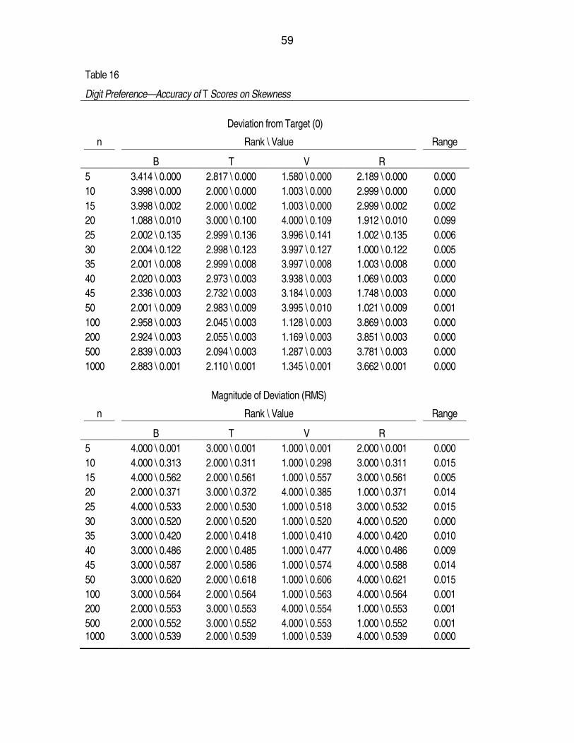
59

Table 16

Digit Preference—Accuracy of T Scores on Skewness



B T V R

5 3.414 \ 0.000 2.817 \ 0.000 1.580 \ 0.000 2.189 \ 0.000 0.000

10 3.998 \ 0.000 2.000 \ 0.000 1.003 \ 0.000 2.999 \ 0.000 0.000

15 3.998 \ 0.002 2.000 \ 0.002 1.003 \ 0.000 2.999 \ 0.002 0.002

20 1.088 \ 0.010 3.000 \ 0.100 4.000 \ 0.109 1.912 \ 0.010 0.099

25 2.002 \ 0.135 2.999 \ 0.136 3.996 \ 0.141 1.002 \ 0.135 0.006

30 2.004 \ 0.122 2.998 \ 0.123 3.997 \ 0.127 1.000 \ 0.122 0.005

35 2.001 \ 0.008 2.999 \ 0.008 3.997 \ 0.008 1.003 \ 0.008 0.000

40 2.020 \ 0.003 2.973 \ 0.003 3.938 \ 0.003 1.069 \ 0.003 0.000

45 2.336 \ 0.003 2.732 \ 0.003 3.184 \ 0.003 1.748 \ 0.003 0.000

50 2.001 \ 0.009 2.983 \ 0.009 3.995 \ 0.010 1.021 \ 0.009 0.001

100 2.958 \ 0.003 2.045 \ 0.003 1.128 \ 0.003 3.869 \ 0.003 0.000

200 2.924 \ 0.003 2.055 \ 0.003 1.169 \ 0.003 3.851 \ 0.003 0.000

500 2.839 \ 0.003 2.094 \ 0.003 1.287 \ 0.003 3.781 \ 0.003 0.000

1000 2.883 \ 0.001 2.110 \ 0.001 1.345 \ 0.001 3.662 \ 0.001 0.000



B T V R

5 4.000 \ 0.001 3.000 \ 0.001 1.000 \ 0.001 2.000 \ 0.001 0.000

10 4.000 \ 0.313 2.000 \ 0.311 1.000 \ 0.298 3.000 \ 0.311 0.015

15 4.000 \ 0.562 2.000 \ 0.561 1.000 \ 0.557 3.000 \ 0.561 0.005

20 2.000 \ 0.371 3.000 \ 0.372 4.000 \ 0.385 1.000 \ 0.371 0.014

25 4.000 \ 0.533 2.000 \ 0.530 1.000 \ 0.518 3.000 \ 0.532 0.015

30 3.000 \ 0.520 2.000 \ 0.520 1.000 \ 0.520 4.000 \ 0.520 0.000

35 3.000 \ 0.420 2.000 \ 0.418 1.000 \ 0.410 4.000 \ 0.420 0.010

40 3.000 \ 0.486 2.000 \ 0.485 1.000 \ 0.477 4.000 \ 0.486 0.009

45 3.000 \ 0.587 2.000 \ 0.586 1.000 \ 0.574 4.000 \ 0.588 0.014

50 3.000 \ 0.620 2.000 \ 0.618 1.000 \ 0.606 4.000 \ 0.621 0.015

100 3.000 \ 0.564 2.000 \ 0.564 1.000 \ 0.563 4.000 \ 0.564 0.001

200 2.000 \ 0.553 3.000 \ 0.553 4.000 \ 0.554 1.000 \ 0.553 0.001

500 2.000 \ 0.552 3.000 \ 0.552 4.000 \ 0.553 1.000 \ 0.552 0.001 1000 3.000 \ 0.539 2.000 \ 0.539 1.000 \ 0.539 4.000 \ 0.539 0.000

60

Table 17

Digit Preference—Accuracy of T Scores on Kurtosis



B T V R

5 1.000 \ 1.153 2.000 \ 1.160 4.000 \ 1.200 3.000 \ 1.162 0.047

10 1.000 \ 1.057 3.000 \ 1.062 4.000 \ 1.095 2.000 \ 0.061 1.034

15 1.000 \ 1.072 3.000 \ 1.076 4.000 \ 1.099 2.000 \ 1.074 0.027

20 1.000 \ 1.082 3.000 \ 1.085 4.000 \ 1.102 2.000 \ 1.083 0.020

25 1.949 \ 1.054 3.000 \ 1.056 4.000 \ 1.073 1.051 \ 1.054 0.019

30 2.000 \ 1.020 3.000 \ 1.023 4.000 \ 1.039 1.000 \ 1.020 0.019

35 2.000 \ 0.976 3.000 \ 0.978 4.000 \ 0.993 1.000 \ 0.975 0.018

40 2.000 \ 0.947 3.000 \ 0.949 4.000 \ 0.964 1.000 \ 0.947 0.017

45 2.000 \ 0.956 3.000 \ 0.958 4.000 \ 0.971 1.000 \ 0.955 0.016

50 2.000 \ 0.969 3.000 \ 0.971 4.000 \ 0.983 1.000 \ 0.968 0.015

100 2.000 \ 0.955 3.000 \ 0.958 4.000 \ 0.974 1.000 \ 0.954 0.020

200 2.000 \ 0.946 3.000 \ 0.940 4.000 \ 0.959 1.000 \ 0.945 0.019

500 2.000 \ 0.940 3.000 \ 0.941 4.000 \ 0.947 1.000 \ 0.939 0.008

1000 2.000 \ 1.083 3.000 \ 1.083 3.999 \ 1.084 1.001 \ 1.083 0.001



B T V R

5 4.000 \ 0.121 3.000 \ 0.121 1.000 \ 0.117 2.000 \ 0.121 0.004

10 1.000 \ 0.328 3.000 \ 0.329 4.000 \ 0.333 2.000 \ 0.329 0.005

15 1.000 \ 0.321 2.000 \ 0.321 4.000 \ 0.323 3.000 \ 0.321 0.002

20 1.000 \ 0.344 3.000 \ 0.345 4.000 \ 0.354 2.000 \ 0.344 0.010

25 4.000 \ 0.433 2.000 \ 0.431 1.000 \ 0.425 3.000 \ 0.432 0.008

30 2.000 \ 0.467 3.000 \ 0.467 4.000 \ 0.472 1.000 \ 0.466 0.006

35 4.000 \ 0.355 3.000 \ 0.355 1.000 \ 0.355 2.000 \ 0.355 0.000

40 3.000 \ 0.433 2.000 \ 0.433 1.000 \ 0.432 4.000 \ 0.434 0.001

45 4.000 \ 0.459 2.000 \ 0.459 1.000 \ 0.458 3.000 \ 0.459 0.001

50 3.000 \ 0.496 2.000 \ 0.496 1.000 \ 0.492 4.000 \ 0.497 0.005

100 2.000 \ 0.481 3.000 \ 0.481 4.000 \ 0.481 1.000 \ 0.481 0.000

200 2.000 \ 0.480 3.000 \ 0.480 4.000 \ 0.480 1.000 \ 0.480 0.000

500 2.000 \ 0.476 3.000 \ 0.476 4.000 \ 0.476 1.000 \ 0.476 0.000 1000 2.000 \ 0.472 3.000 \ 0.472 4.000 \ 0.472 1.000 \ 0.472 0.000

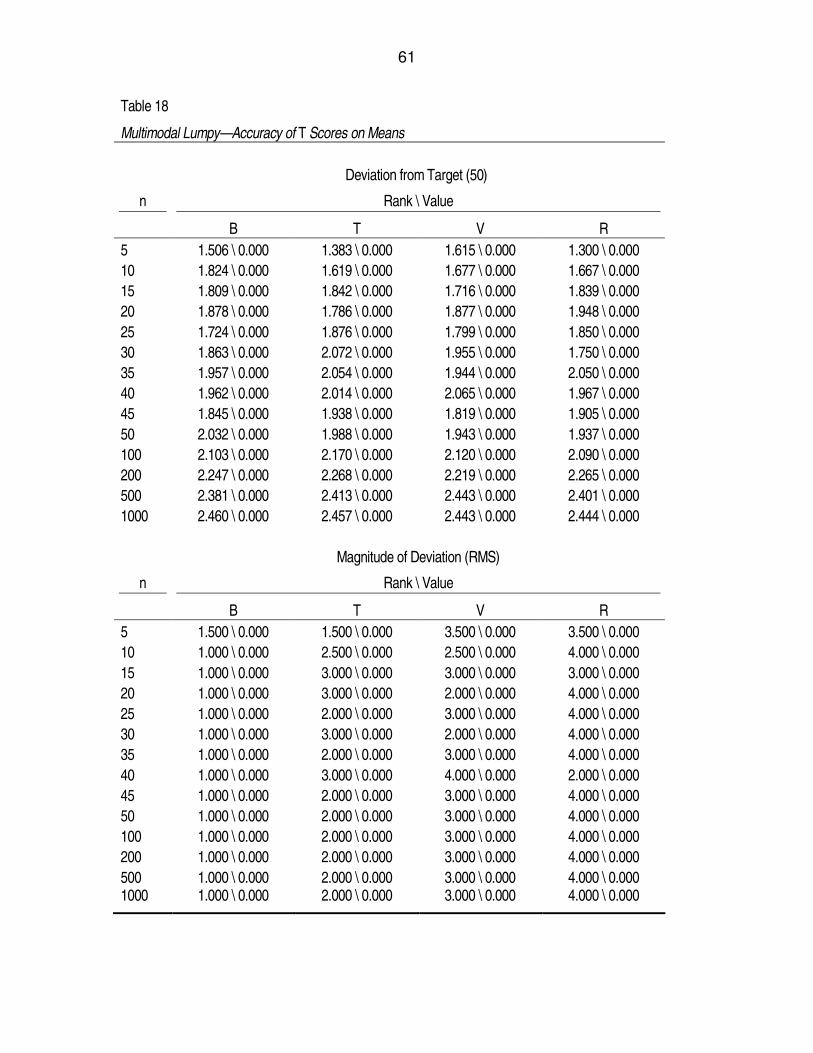
61

Table 18

Multimodal Lumpy—Accuracy of T Scores on Means


n Rank \ Value

B T V R

5 1.506 \ 0.000 1.383 \ 0.000 1.615 \ 0.000 1.300 \ 0.000

10 1.824 \ 0.000 1.619 \ 0.000 1.677 \ 0.000 1.667 \ 0.000

15 1.809 \ 0.000 1.842 \ 0.000 1.716 \ 0.000 1.839 \ 0.000

20 1.878 \ 0.000 1.786 \ 0.000 1.877 \ 0.000 1.948 \ 0.000

25 1.724 \ 0.000 1.876 \ 0.000 1.799 \ 0.000 1.850 \ 0.000

30 1.863 \ 0.000 2.072 \ 0.000 1.955 \ 0.000 1.750 \ 0.000

35 1.957 \ 0.000 2.054 \ 0.000 1.944 \ 0.000 2.050 \ 0.000

40 1.962 \ 0.000 2.014 \ 0.000 2.065 \ 0.000 1.967 \ 0.000

45 1.845 \ 0.000 1.938 \ 0.000 1.819 \ 0.000 1.905 \ 0.000

50 2.032 \ 0.000 1.988 \ 0.000 1.943 \ 0.000 1.937 \ 0.000

100 2.103 \ 0.000 2.170 \ 0.000 2.120 \ 0.000 2.090 \ 0.000

200 2.247 \ 0.000 2.268 \ 0.000 2.219 \ 0.000 2.265 \ 0.000

500 2.381 \ 0.000 2.413 \ 0.000 2.443 \ 0.000 2.401 \ 0.000

1000 2.460 \ 0.000 2.457 \ 0.000 2.443 \ 0.000 2.444 \ 0.000


n Rank \ Value

B T V R

5 1.500 \ 0.000 1.500 \ 0.000 3.500 \ 0.000 3.500 \ 0.000

10 1.000 \ 0.000 2.500 \ 0.000 2.500 \ 0.000 4.000 \ 0.000

15 1.000 \ 0.000 3.000 \ 0.000 3.000 \ 0.000 3.000 \ 0.000

20 1.000 \ 0.000 3.000 \ 0.000 2.000 \ 0.000 4.000 \ 0.000

25 1.000 \ 0.000 2.000 \ 0.000 3.000 \ 0.000 4.000 \ 0.000

30 1.000 \ 0.000 3.000 \ 0.000 2.000 \ 0.000 4.000 \ 0.000

35 1.000 \ 0.000 2.000 \ 0.000 3.000 \ 0.000 4.000 \ 0.000

40 1.000 \ 0.000 3.000 \ 0.000 4.000 \ 0.000 2.000 \ 0.000

45 1.000 \ 0.000 2.000 \ 0.000 3.000 \ 0.000 4.000 \ 0.000

50 1.000 \ 0.000 2.000 \ 0.000 3.000 \ 0.000 4.000 \ 0.000

100 1.000 \ 0.000 2.000 \ 0.000 3.000 \ 0.000 4.000 \ 0.000

200 1.000 \ 0.000 2.000 \ 0.000 3.000 \ 0.000 4.000 \ 0.000

500 1.000 \ 0.000 2.000 \ 0.000 3.000 \ 0.000 4.000 \ 0.000 1000 1.000 \ 0.000 2.000 \ 0.000 3.000 \ 0.000 4.000 \ 0.000

62

Table 19

Multimodal Lumpy—Accuracy of T Scores on Standard Deviations



B T V R

5 1.000 \ 1.963 3.000 \ 2.154 4.000 \ 3.351 2.000 \ 2.065 1.388

10 1.000 \ 1.123 3.000 \ 1.258 4.000 \ 2.151 2.000 \ 1.146 1.028

15 2.000 \ 0.810 3.000 \ 0.917 4.000 \ 1.636 1.000 \ 0.809 0.827

20 2.000 \ 0.643 3.000 \ 0.733 4.000 \ 1.341 1.000 \ 0.631 0.710

25 2.000 \ 0.537 3.000 \ 0.615 4.000 \ 1.145 1.000 \ 0.520 0.625

30 2.000 \ 0.464 3.000 \ 0.533 4.000 \ 1.005 1.000 \ 0.444 0.561

35 2.000 \ 0.410 3.000 \ 0.471 4.000 \ 0.898 1.000 \ 0.388 0.510

40 2.000 \ 0.368 3.000 \ 0.424 4.000 \ 0.815 1.000 \ 0.346 0.469

45 2.000 \ 0.334 3.000 \ 0.386 4.000 \ 0.747 1.000 \ 0.311 0.436

50 2.000 \ 0.307 3.000 \ 0.355 4.000 \ 0.691 1.000 \ 0.285 0.406

100 2.000 \ 0.178 3.000 \ 0.206 4.000 \ 0.411 1.000 \ 0.158 0.253

200 2.000 \ 0.105 3.000 \ 0.122 4.000 \ 0.242 1.000 \ 0.009 0.233

500 2.000 \ 0.006 3.000 \ 0.006 4.000 \ 0.123 1.000 \ 0.005 0.118

1000 2.000 \ 0.004 3.000 \ 0.004 4.000 \ 0.008 1.000 \ 0.004 0.004



B T V R

5 4.000 \ 0.118 3.000 \ 0.115 2.000 \ 0.114 1.000 \ 0.009 0.109

10 4.000 \ 0.003 3.000 \ 0.003 2.000 \ 0.003 1.000 \ 0.002 0.001

15 3.000 \ 0.002 4.000 \ 0.002 2.000 \ 0.002 1.000 \ 0.002 0.000

20 3.000 \ 0.002 4.000 \ 0.002 2.000 \ 0.002 1.000 \ 0.001 0.001

25 3.000 \ 0.002 4.000 \ 0.002 2.000 \ 0.002 1.000 \ 0.002 0.000

30 3.000 \ 0.002 4.000 \ 0.002 2.000 \ 0.002 1.000 \ 0.001 0.001

35 3.000 \ 0.001 4.000 \ 0.001 2.000 \ 0.001 1.000 \ 0.001 0.000

40 3.000 \ 0.001 4.000 \ 0.001 2.000 \ 0.001 1.000 \ 0.001 0.000

45 4.000 \ 0.002 3.000 \ 0.002 2.000 \ 0.002 1.000 \ 0.001 0.001

50 4.000 \ 0.001 3.000 \ 0.001 2.000 \ 0.001 1.000 \ 0.001 0.000

100 4.000 \ 0.001 3.000 \ 0.001 2.000 \ 0.001 1.000 \ 0.001 0.000

200 4.000 \ 0.000 3.000 \ 0.000 2.000 \ 0.000 1.000 \ 0.000 0.000

500 4.000 \ 0.000 3.000 \ 0.000 2.000 \ 0.000 1.000 \ 0.000 0.000 1000 4.000 \ 0.000 3.000 \ 0.000 2.000 \ 0.000 1.000 \ 0.000 0.000

63

Table 20

Multimodal Lumpy—Accuracy of T Scores on Skewness



B T V R

5 3.989 \ 0.000 2.996 \ 0.000 1.012 \ 0.000 2.003 \ 0.000 0.000

10 1.399 \ 0.003 2.912 \ 0.003 3.742 \ 0.003 1.948 \ 0.003 0.000

15 1.000 \ 0.009 3.000 \ 0.009 4.000 \ 0.009 2.000 \ 0.009 0.000

20 1.565 \ 0.128 2.999 \ 0.129 3.996 \ 0.134 1.439 \ 0.128 0.006

25 1.994 \ 0.121 2.999 \ 0.122 3.998 \ 0.128 1.009 \ 0.121 0.007

30 2.005 \ 0.006 2.998 \ 0.006 3.993 \ 0.007 1.004 \ 0.006 0.001

35 2.853 \ 0.118 2.104 \ 0.115 1.429 \ 0.009 3.614 \ 0.118 0.109

40 3.024 \ 0.120 2.001 \ 0.118 1.004 \ 0.100 3.972 \ 0.121 0.021

45 2.191 \ 0.005 2.735 \ 0.005 3.402 \ 0.006 1.673 \ 0.005 0.001

50 2.001 \ 0.144 2.999 \ 0.145 3.998 \ 0.149 1.002 \ 0.144 0.005

100 2.928 \ 0.003 2.054 \ 0.003 1.168 \ 0.003 3.851 \ 0.003 0.000

200 2.925 \ 0.003 2.062 \ 0.003 1.186 \ 0.003 3.827 \ 0.003 0.000

500 2.917 \ 0.003 2.079 \ 0.003 1.207 \ 0.003 3.797 \ 0.003 0.000

1000 2.884 \ 0.003 2.104 \ 0.003 1.286 \ 0.003 3.726 \ 0.003 0.000



B T V R

5 4.000 \ 0.010 3.000 \ 0.009 1.000 \ 0.009 2.000 \ 0.009 0.001

10 4.000 \ 0.572 2.000 \ 0.567 1.000 \ 0.534 3.000 \ 0.568 0.038

15 4.000 \ 0.490 2.000 \ 0.486 1.000 \ 0.461 3.000 \ 0.489 0.029

20 4.000 \ 0.684 2.000 \ 0.682 1.000 \ 0.672 3.000 \ 0.684 0.012

25 4.000 \ 0.566 2.000 \ 0.564 1.000 \ 0.553 3.000 \ 0.566 0.013

30 2.000 \ 0.399 3.000 \ 0.399 4.000 \ 0.401 1.000 \ 0.399 0.002

35 2.000 \ 0.477 3.000 \ 0.478 4.000 \ 0.482 1.000 \ 0.477 0.005

40 2.000 \ 0.588 3.000 \ 0.589 4.000 \ 0.596 1.000 \ 0.588 0.008

45 2.000 \ 0.448 3.000 \ 0.448 4.000 \ 0.449 1.000 \ 0.447 0.002

50 2.000 \ 0.484 3.000 \ 0.484 4.000 \ 0.485 1.000 \ 0.480 0.005

100 3.000 \ 0.559 2.000 \ 0.559 1.000 \ 0.559 4.000 \ 0.559 0.000

200 2.000 \ 0.556 3.000 \ 0.556 4.000 \ 0.557 1.000 \ 0.556 0.001

500 2.000 \ 0.550 3.000 \ 0.550 4.000 \ 0.550 1.000 \ 0.550 0.000 1000 2.000 \ 0.561 3.000 \ 0.561 4.000 \ 0.561 1.000 \ 0.561 0.000

64

Table 21

Multimodal Lumpy—Accuracy of T Scores on Kurtosis



B T V R

5 1.000 \ 1.150 2.000 \ 1.157 4.000 \ 1.197 3.000 \ 1.158 0.047

10 1.000 \ 1.043 3.000 \ 1.047 4.000 \ 1.077 2.000 \ 1.046 0.034

15 1.000 \ 1.022 3.000 \ 1.026 4.000 \ 1.050 2.000 \ 1.024 0.028

20 1.000 \ 1.042 3.000 \ 1.045 4.000 \ 1.064 2.000 \ 1.043 0.022

25 1.999 \ 1.083 3.000 \ 1.086 4.000 \ 1.101 1.001 \ 1.083 0.018

30 2.000 \ 1.108 3.000 \ 1.110 4.000 \ 1.123 1.000 \ 1.107 0.016

35 2.000 \ 1.049 3.000 \ 1.052 4.000 \ 1.070 1.000 \ 1.048 0.022

40 2.000 \ 1.021 3.000 \ 1.024 4.000 \ 1.044 1.000 \ 1.020 0.024

45 2.000 \ 1.105 3.000 \ 1.107 4.000 \ 1.117 1.000 \ 1.105 0.012

50 2.000 \ 1.072 3.000 \ 1.074 3.999 \ 1.084 1.001 \ 1.072 0.012

100 2.000 \ 0.960 3.000 \ 0.962 4.000 \ 0.978 1.000 \ 0.958 0.020

200 2.000 \ 0.950 3.000 \ 0.952 4.000 \ 0.962 1.000 \ 0.949 0.013

500 2.000 \ 0.943 3.000 \ 0.944 4.000 \ 0.950 1.000 \ 0.942 0.008

1000 2.000 \ 0.942 3.000 \ 0.942 4.000 \ 0.942 1.000 \ 0.941 0.001



B T V R

5 4.000 \ 0.121 3.000 \ 0.121 1.000 \ 0.117 2.000 \ 0.121 0.004

10 4.000 \ 0.410 2.000 \ 0.403 1.000 \ 0.390 3.000 \ 0.403 0.020

15 4.000 \ 0.426 2.000 \ 0.424 1.000 \ 0.415 3.000 \ 0.425 0.011

20 1.000 \ 0.480 3.000 \ 0.481 4.000 \ 0.485 2.000 \ 0.480 0.005

25 2.000 \ 0.416 3.000 \ 0.416 4.000 \ 0.420 1.000 \ 0.416 0.004

30 2.000 \ 0.348 3.000 \ 0.348 4.000 \ 0.355 1.000 \ 0.347 0.008

35 2.000 \ 0.435 3.000 \ 0.435 4.000 \ 0.439 1.000 \ 0.435 0.004

40 2.000 \ 0.463 3.000 \ 0.464 4.000 \ 0.473 1.000 \ 0.463 0.010

45 2.000 \ 0.399 3.000 \ 0.399 4.000 \ 0.400 1.000 \ 0.399 0.001

50 2.000 \ 0.432 3.000 \ 0.432 4.000 \ 0.434 1.000 \ 0.432 0.002

100 1.000 \ 0.472 3.000 \ 0.472 4.000 \ 0.472 2.000 \ 0.472 0.000

200 2.000 \ 0.475 3.000 \ 0.475 4.000 \ 0.475 1.000 \ 0.474 0.001

500 2.000 \ 0.471 3.000 \ 0.471 4.000 \ 0.471 1.000 \ 0.471 0.000 1000 2.000 \ 0.478 3.000 \ 0.478 4.000 \ 0.478 1.000 \ 0.478 0.000

65

Table 22

Mass at Zero with Gap—Accuracy of T Scores on Means


n Rank \ Value

B T V R

5 1.190 \ 0.000 1.342 \ 0.000 1.561 \ 0.000 1.001 \ 0.000

10 1.989 \ 0.000 1.520 \ 0.000 2.024 \ 0.000 2.105 \ 0.000

15 1.619 \ 0.000 2.125 \ 0.000 2.031 \ 0.000 1.882 \ 0.000

20 1.535 \ 0.000 1.665 \ 0.000 2.191 \ 0.000 2.268 \ 0.000

25 2.016 \ 0.000 1.550 \ 0.000 1.807 \ 0.000 2.747 \ 0.000

30 2.103 \ 0.000 2.111 \ 0.000 2.396 \ 0.000 2.036 \ 0.000

35 2.618 \ 0.000 1.833 \ 0.000 2.457 \ 0.000 1.926 \ 0.000

40 2.503 \ 0.000 1.926 \ 0.000 1.804 \ 0.000 2.093 \ 0.000

45 2.514 \ 0.000 2.011 \ 0.000 1.863 \ 0.000 2.242 \ 0.000

50 2.410 \ 0.000 2.026 \ 0.000 1.932 \ 0.000 2.659 \ 0.000

100 2.350 \ 0.000 2.218 \ 0.000 2.594 \ 0.000 2.267 \ 0.000

200 2.352 \ 0.000 2.365 \ 0.000 2.273 \ 0.000 2.695 \ 0.000

500 2.542 \ 0.000 2.393 \ 0.000 2.161 \ 0.000 2.814 \ 0.000

1000 2.538 \ 0.000 2.331 \ 0.000 2.547 \ 0.000 2.523 \ 0.000


n Rank \ Value

B T V R

5 2.000 \ 0.000 2.000 \ 0.000 2.000 \ 0.000 4.000 \ 0.000

10 1.000 \ 0.000 2.000 \ 0.000 3.000 \ 0.000 4.000 \ 0.000

15 2.500 \ 0.000 4.000 \ 0.000 2.500 \ 0.000 1.000 \ 0.000

20 3.000 \ 0.000 1.000 \ 0.000 2.000 \ 0.000 4.000 \ 0.000

25 1.000 \ 0.000 2.000 \ 0.000 4.000 \ 0.000 3.000 \ 0.000

30 3.000 \ 0.000 1.000 \ 0.000 2.000 \ 0.000 4.000 \ 0.000

35 3.000 \ 0.000 2.000 \ 0.000 4.000 \ 0.000 1.000 \ 0.000

40 2.000 \ 0.000 1.000 \ 0.000 3.000 \ 0.000 4.000 \ 0.000

45 1.000 \ 0.000 3.000 \ 0.000 4.000 \ 0.000 2.000 \ 0.000

50 1.000 \ 0.000 3.000 \ 0.000 2.000 \ 0.000 4.000 \ 0.000

100 1.000 \ 0.000 3.000 \ 0.000 2.000 \ 0.000 4.000 \ 0.000

200 1.000 \ 0.000 2.000 \ 0.000 3.000 \ 0.000 4.000 \ 0.000

500 2.000 \ 0.000 1.000 \ 0.000 3.000 \ 0.000 4.000 \ 0.000 1000 2.000 \ 0.000 4.000 \ 0.000 3.000 \ 0.000 1.000 \ 0.000

66

Table 23

Mass at Zero with Gap—Accuracy of T Scores on Standard Deviations



B T V R

5 1.000 \ 6.281 2.186 \ 6.372 2.779 \ 6.937 1.593 \ 6.331 0.656

10 1.000 \ 4.589 2.721 \ 4.678 3.581 \ 5.255 1.860 \ 4.608 0.666

15 1.382 \ 3.898 2.909 \ 3.976 3.864 \ 4.491 1.572 \ 3.900 0.593

20 1.957 \ 3.255 2.987 \ 3.323 3.981 \ 3.786 1.036 \ 3.246 0.540

25 2.000 \ 2.976 3.000 \ 3.035 4.000 \ 3.444 1.000 \ 2.962 0.482

30 2.000 \ 2.940 3.000 \ 2.993 4.000 \ 3.358 1.000 \ 2.925 0.433

35 1.999 \ 3.215 2.999 \ 3.262 3.998 \ 3.589 1.000 \ 3.199 0.390

40 2.000 \ 3.163 2.999 \ 3.206 3.999 \ 3.506 1.000 \ 3.146 0.360

45 2.000 \ 3.113 3.000 \ 3.153 4.000 \ 3.430 1.000 \ 3.096 0.334

50 2.000 \ 3.078 3.000 \ 3.114 4.000 \ 3.373 1.000 \ 3.060 0.313

100 2.000 \ 2.909 3.000 \ 2.931 4.000 \ 3.089 1.000 \ 2.893 0.196

200 2.000 \ 2.802 3.000 \ 2.815 4.000 \ 2.909 1.000 \ 2.790 0.119

500 2.000 \ 2.759 3.000 \ 2.765 4.000 \ 2.811 1.000 \ 2.752 0.059

1000 1.957 \ 2.746 2.810 \ 2.750 4.000 \ 2.776 1.233 \ 2.743 0.033



B T V R

5 4.000 \ 2.750 3.000 \ 2.717 2.000 \ 2.687 1.000 \ 2.283 0.467

10 4.000 \ 2.676 3.000 \ 2.668 2.000 \ 2.634 1.000 \ 2.362 0.314

15 3.000 \ 0.904 4.000 \ 0.906 2.000 \ 0.899 1.000 \ 0.867 0.037

20 4.000 \ 0.645 3.000 \ 0.644 2.000 \ 0.642 1.000 \ 0.626 0.019

25 4.000 \ 0.520 3.000 \ 0.519 2.000 \ 0.519 1.000 \ 0.511 0.009

30 4.000 \ 0.524 3.000 \ 0.523 2.000 \ 0.523 1.000 \ 0.517 0.007

35 4.000 \ 0.826 3.000 \ 0.824 2.000 \ 0.824 1.000 \ 0.814 0.012

40 4.000 \ 0.623 3.000 \ 0.623 2.000 \ 0.622 1.000 \ 0.617 0.006

45 4.000 \ 0.681 3.000 \ 0.680 2.000 \ 0.680 1.000 \ 0.677 0.004

50 4.000 \ 0.662 3.000 \ 0.661 2.000 \ 0.661 1.000 \ 0.658 0.004

100 1.000 \ 0.348 2.000 \ 0.348 4.000 \ 0.348 3.000 \ 0.348 0.000

200 1.000 \ 0.264 2.000 \ 0.265 3.000 \ 0.265 4.000 \ 0.265 0.001

500 1.000 \ 0.169 2.000 \ 0.169 3.000 \ 0.169 4.000 \ 0.170 0.001 1000 1.000 \ 0.119 2.000 \ 0.119 4.000 \ 0.119 3.000 \ 0.119 0.000

67

Table 24

Mass at Zero with Gap—Accuracy of T Scores on Skewness



B T V R

5 4.000 \ 0.719 3.000 \ 0.718 1.000 \ 0.715 2.000 \ 0.718 0.004

10 4.000 \ 0.688 2.000 \ 0.687 1.000 \ 0.684 3.000 \ 0.687 0.004

15 3.999 \ 0.675 2.000 \ 0.675 1.000 \ 0.672 3.000 \ 0.675 0.003

20 4.000 \ 0.761 2.000 \ 0.760 1.000 \ 0.753 3.000 \ 0.761 0.008

25 3.998 \ 0.774 2.000 \ 0.772 1.000 \ 0.764 3.002 \ 0.774 0.010

30 3.056 \ 0.808 2.000 \ 0.806 1.000 \ 0.794 3.944 \ 0.808 0.014

35 2.999 \ 0.692 2.000 \ 0.691 1.001 \ 0.689 4.000 \ 0.692 0.003

40 3.002 \ 0.676 2.000 \ 0.676 1.001 \ 0.674 3.997 \ 0.676 0.002

45 2.999 \ 0.676 1.999 \ 0.676 1.002 \ 0.674 3.999 \ 0.676 0.002

50 2.997 \ 0.694 2.003 \ 0.694 1.001 \ 0.692 3.997 \ 0.695 0.003

100 3.000 \ 0.701 2.000 \ 0.701 1.000 \ 0.699 4.000 \ 0.701 0.002

200 3.000 \ 0.747 2.000 \ 0.747 1.000 \ 0.743 4.000 \ 0.748 0.005

500 3.000 \ 0.749 2.000 \ 0.749 1.000 \ 0.746 4.000 \ 0.749 0.003

1000 2.999 \ 0.701 2.000 \ 0.700 1.001 \ 0.700 3.999 \ 0.701 0.001



B T V R

5 4.000 \ 0.491 3.000 \ 0.491 1.000 \ 0.491 2.000 \ 0.491 0.000

10 4.000 \ 0.575 2.000 \ 0.574 1.000 \ 0.573 3.000 \ 0.574 0.002

15 1.000 \ 0.676 3.000 \ 0.676 4.000 \ 0.677 2.000 \ 0.676 0.001

20 1.000 \ 0.692 3.000 \ 0.692 4.000 \ 0.693 2.000 \ 0.692 0.001

25 2.000 \ 0.626 3.000 \ 0.626 4.000 \ 0.632 1.000 \ 0.625 0.007

30 1.000 \ 0.751 3.000 \ 0.753 4.000 \ 0.764 2.000 \ 0.751 0.002

35 2.000 \ 0.684 3.000 \ 0.685 4.000 \ 0.686 1.000 \ 0.684 0.002

40 2.000 \ 0.658 3.000 \ 0.658 4.000 \ 0.659 1.000 \ 0.658 0.001

45 2.000 \ 0.686 3.000 \ 0.686 4.000 \ 0.687 1.000 \ 0.686 0.001

50 2.000 \ 0.693 3.000 \ 0.693 4.000 \ 0.694 1.000 \ 0.693 0.001

100 2.000 \ 0.714 3.000 \ 0.714 4.000 \ 0.714 1.000 \ 0.714 0.000

200 2.000 \ 0.681 3.000 \ 0.682 4.000 \ 0.685 1.000 \ 0.681 0.004

500 2.000 \ 0.691 3.000 \ 0.691 4.000 \ 0.693 1.000 \ 0.691 0.002 1000 2.000 \ 0.715 3.000 \ 0.715 4.000 \ 0.715 1.000 \ 0.715 0.000

68

Table 25

Mass at Zero with Gap—Accuracy of T Scores on Kurtosis



B T V R

5 1.000 \ 0.144 2.000 \ 0.145 4.000 \ 0.150 3.000 \ 0.145 0.006

10 1.000 \ 0.183 2.500 \ 0.184 4.000 \ 0.190 2.500 \ 0.184 0.007

15 1.001 \ 0.199 3.000 \ 0.200 3.999 \ 0.206 2.000 \ 0.200 0.007

20 1.001 \ 0.517 3.000 \ 0.518 3.999 \ 0.528 2.000 \ 0.517 0.011

25 1.000 \ 0.846 3.000 \ 0.848 4.000 \ 0.858 2.000 \ 0.846 0.012

30 1.742 \ 0.779 3.000 \ 0.782 4.000 \ 0.797 1.258 \ 0.780 0.018

35 2.000 \ 0.180 2.999 \ 0.181 4.000 \ 0.185 1.000 \ 0.180 0.005

40 1.997 \ 0.202 3.000 \ 0.203 3.999 \ 0.206 1.003 \ 0.202 0.004

45 2.000 \ 0.199 3.000 \ 0.200 3.997 \ 0.203 1.002 \ 0.199 0.004

50 2.001 \ 0.172 2.999 \ 0.172 3.998 \ 0.175 1.002 \ 0.171 0.004

100 2.000 \ 0.163 3.000 \ 0.164 3.998 \ 0.166 1.001 \ 0.163 0.003

200 2.000 \ 0.423 3.000 \ 0.424 4.000 \ 0.430 1.000 \ 0.423 0.007

500 2.000 \ 0.421 3.000 \ 0.422 4.000 \ 0.425 1.000 \ 0.421 0.004

1000 2.000 \ 0.164 2.999 \ 0.164 3.999 \ 0.164 1.002 \ 0.164 0.000



B T V R

5 1.000 \ 0.807 2.000 \ 0.809 4.000 \ 0.819 3.000 \ 0.809 0.012

10 1.000 \ 0.675 3.000 \ 0.679 4.000 \ 0.705 2.000 \ 0.678 0.030

15 1.000 \ 0.667 3.000 \ 0.670 4.000 \ 0.691 2.000 \ 0.669 0.024

20 1.000 \ 0.615 3.000 \ 0.617 4.000 \ 0.628 2.000 \ 0.615 0.013

25 2.000 \ 0.945 3.000 \ 0.945 4.000 \ 0.951 1.000 \ 0.945 0.006

30 1.000 \ 0.900 3.000 \ 0.902 4.000 \ 0.913 2.000 \ 0.900 0.013

35 2.000 \ 0.740 3.000 \ 0.740 4.000 \ 0.745 1.000 \ 0.740 0.005

40 2.000 \ 0.754 3.000 \ 0.755 4.000 \ 0.756 1.000 \ 0.754 0.002

45 2.000 \ 0.715 3.000 \ 0.716 4.000 \ 0.724 1.000 \ 0.715 0.009

50 2.000 \ 0.611 3.000 \ 0.613 4.000 \ 0.622 1.000 \ 0.611 0.011

100 2.000 \ 0.687 3.000 \ 0.688 4.000 \ 0.691 1.000 \ 0.687 0.004

200 2.000 \ 0.940 3.000 \ 0.940 4.000 \ 0.942 1.000 \ 0.940 0.002

500 2.000 \ 0.945 3.000 \ 0.945 4.000 \ 0.946 1.000 \ 0.945 0.001 1000 2.000 \ 0.657 3.000 \ 0.657 4.000 \ 0.657 1.000 \ 0.656 0.001

69

Table 26

Extreme Asymmetric, Decay—Accuracy of T Scores on Means


n Rank \ Value

B T V R

5 1.872 \ 0.000 1.520 \ 0.000 1.575 \ 0.000 1.032 \ 0.000

10 1.748 \ 0.000 1.604 \ 0.000 1.930 \ 0.000 2.158 \ 0.000

15 1.703 \ 0.000 1.945 \ 0.000 1.967 \ 0.000 1.854 \ 0.000

20 2.455 \ 0.000 1.720 \ 0.000 2.076 \ 0.000 1.546 \ 0.000

25 1.918 \ 0.000 1.684 \ 0.000 1.823 \ 0.000 2.114 \ 0.000

30 2.150 \ 0.000 1.895 \ 0.000 2.018 \ 0.000 1.992 \ 0.000

35 2.203 \ 0.000 2.284 \ 0.000 2.063 \ 0.000 2.092 \ 0.000

40 1.705 \ 0.000 2.564 \ 0.000 1.867 \ 0.000 2.313 \ 0.000

45 2.109 \ 0.000 2.300 \ 0.000 1.912 \ 0.000 1.831 \ 0.000

50 1.890 \ 0.000 2.431 \ 0.000 2.297 \ 0.000 1.955 \ 0.000

100 2.272 \ 0.000 2.329 \ 0.000 2.166 \ 0.000 2.466 \ 0.000

200 2.503 \ 0.000 2.275 \ 0.000 2.392 \ 0.000 2.389 \ 0.000

500 2.293 \ 0.000 2.640 \ 0.000 2.485 \ 0.000 2.444 \ 0.000

1000 2.528 \ 0.000 2.582 \ 0.000 2.447 \ 0.000 2.379 \ 0.000


n Rank \ Value

B T V R

5 2.000 \ 0.000 2.000 \ 0.000 2.000 \ 0.000 4.000 \ 0.000

10 1.000 \ 0.000 3.000 \ 0.000 4.000 \ 0.000 2.000 \ 0.000

15 3.000 \ 0.000 4.000 \ 0.000 1.000 \ 0.000 2.000 \ 0.000

20 3.000 \ 0.000 4.000 \ 0.000 1.500 \ 0.000 1.500 \ 0.000

25 1.000 \ 0.000 2.000 \ 0.000 3.000 \ 0.000 4.000 \ 0.000

30 1.000 \ 0.000 2.000 \ 0.000 3.000 \ 0.000 4.000 \ 0.000

35 1.000 \ 0.000 2.000 \ 0.000 3.000 \ 0.000 4.000 \ 0.000

40 3.000 \ 0.000 2.000 \ 0.000 1.000 \ 0.000 4.000 \ 0.000

45 1.000 \ 0.000 2.000 \ 0.000 3.000 \ 0.000 4.000 \ 0.000

50 1.000 \ 0.000 2.000 \ 0.000 3.000 \ 0.000 4.000 \ 0.000

100 1.000 \ 0.000 2.000 \ 0.000 3.000 \ 0.000 4.000 \ 0.000

200 1.000 \ 0.000 2.000 \ 0.000 3.000 \ 0.000 4.000 \ 0.000

500 1.000 \ 0.000 2.000 \ 0.000 3.000 \ 0.000 4.000 \ 0.000 1000 1.000 \ 0.000 2.000 \ 0.000 3.000 \ 0.000 4.000 \ 0.000

70

Table 27

Extreme Asymmetric, Decay—Accuracy of T Scores on Standard Deviations



B T V R

5 1.000 \ 3.410 2.873 \ 3.566 3.810 \ 4.547 1.937 \ 3.494 1.137

10 1.000 \ 2.171 2.995 \ 2.287 3.993 \ 3.059 1.998 \ 2.190 0.888

15 1.974 \ 1.801 3.000 \ 1.892 4.000 \ 2.511 1.026 \ 1.798 0.713

20 2.000 \ 1.611 3.000 \ 1.687 4.000 \ 2.207 1.000 \ 1.599 0.608

25 2.000 \ 1.495 3.000 \ 1.560 4.000 \ 2.011 1.000 \ 1.480 0.531

30 2.000 \ 1.319 3.000 \ 1.376 4.000 \ 1.779 1.000 \ 1.301 0.478

35 2.000 \ 1.260 3.000 \ 1.312 4.000 \ 1.674 1.000 \ 1.241 0.433

40 2.000 \ 1.228 3.000 \ 1.275 4.000 \ 1.604 1.000 \ 1.209 0.395

45 2.000 \ 1.203 3.000 \ 1.246 4.000 \ 1.548 1.000 \ 1.184 0.364

50 2.000 \ 1.184 3.000 \ 1.224 4.000 \ 1.504 1.000 \ 1.165 0.339

100 2.000 \ 1.129 3.000 \ 1.152 4.000 \ 1.317 1.000 \ 1.114 0.203

200 2.000 \ 1.055 3.000 \ 1.068 4.000 \ 1.162 1.000 \ 1.044 0.118

500 2.000 \ 1.017 3.000 \ 1.022 4.000 \ 1.066 1.000 \ 1.010 0.056

1000 2.022 \ 1.003 2.911 \ 1.006 4.000 \ 1.030 1.067 \ 1.001 0.029



B T V R

5 4.000 \ 0.307 3.000 \ 0.303 2.000 \ 0.300 1.000 \ 0.257 0.050

10 4.000 \ 0.460 3.000 \ 0.459 2.000 \ 0.454 1.000 \ 0.414 0.046

15 4.000 \ 0.365 3.000 \ 0.365 2.000 \ 0.362 1.000 \ 0.340 0.025

20 4.000 \ 0.451 3.000 \ 0.450 2.000 \ 0.447 1.000 \ 0.428 0.023

25 4.000 \ 0.301 3.000 \ 0.300 2.000 \ 0.299 1.000 \ 0.287 0.014

30 4.000 \ 0.283 3.000 \ 0.283 2.000 \ 0.282 1.000 \ 0.273 0.010

35 4.000 \ 0.251 3.000 \ 0.250 2.000 \ 0.249 1.000 \ 0.240 0.011

40 4.000 \ 0.251 3.000 \ 0.250 2.000 \ 0.249 1.000 \ 0.239 0.012

45 4.000 \ 0.215 3.000 \ 0.215 2.000 \ 0.214 1.000 \ 0.209 0.006

50 4.000 \ 0.215 3.000 \ 0.215 2.000 \ 0.214 1.000 \ 0.209 0.006

100 4.000 \ 0.176 3.000 \ 0.175 2.000 \ 0.175 1.000 \ 0.174 0.002

200 4.000 \ 0.121 3.000 \ 0.120 2.000 \ 0.120 1.000 \ 0.119 0.002

500 4.000 \ 0.008 3.000 \ 0.008 2.000 \ 0.008 1.000 \ 0.008 0.000 1000 2.000 \ 0.005 3.000 \ 0.005 4.000 \ 0.005 1.000 \ 0.005 0.000

71

Table 28

Extreme Asymmetric, Decay—Accuracy of T Scores on Skewness



B T V R

5 4.000 \ 0.668 3.000 \ 0.666 1.000 \ 0.653 2.000 \ 0.665 0.015

10 4.000 \ 0.647 2.000 \ 0.645 1.000 \ 0.635 3.000 \ 0.645 0.012

15 3.998 \ 0.635 2.000 \ 0.633 1.001 \ 0.625 3.001 \ 0.634 0.010

20 3.994 \ 0.605 2.000 \ 0.604 1.000 \ 0.597 3.006 \ 0.605 0.008

25 3.000 \ 0.578 2.000 \ 0.577 1.000 \ 0.571 3.999 \ 0.578 0.007

30 3.000 \ 0.323 2.000 \ 0.322 1.000 \ 0.315 4.000 \ 0.323 0.008

35 3.000 \ 0.235 2.000 \ 0.234 1.001 \ 0.226 3.999 \ 0.235 0.009

40 3.000 \ 0.156 2.000 \ 0.155 1.000 \ 0.146 4.000 \ 0.157 0.011

45 3.000 \ 0.101 2.001 \ 0.010 1.001 \ 0.010 4.000 \ 0.102 0.092

50 3.000 \ 0.009 2.000 \ 0.009 1.000 \ 0.008 3.999 \ 0.009 0.001

100 3.000 \ 0.591 2.000 \ 0.590 1.000 \ 0.588 4.000 \ 0.591 0.003

200 3.000 \ 0.501 2.000 \ 0.500 1.000 \ 0.493 4.000 \ 0.502 0.009

500 3.000 \ 0.505 2.000 \ 0.504 1.000 \ 0.501 4.000 \ 0.505 0.004

1000 3.000 \ 0.505 2.000 \ 0.505 1.000 \ 0.503 4.000 \ 0.506 0.003



B T V R

5 4.000 \ 0.208 3.000 \ 0.208 1.000 \ 0.207 2.000 \ 0.208 0.001

10 1.000 \ 0.587 3.000 \ 0.588 4.000 \ 0.599 2.000 \ 0.588 0.012

15 4.000 \ 0.612 3.000 \ 0.612 1.000 \ 0.611 2.000 \ 0.612 0.001

20 3.000 \ 0.611 2.000 \ 0.611 4.000 \ 0.611 1.000 \ 0.611 0.000

25 2.000 \ 0.594 3.000 \ 0.594 4.000 \ 0.596 1.000 \ 0.594 0.002

30 2.000 \ 0.551 3.000 \ 0.551 4.000 \ 0.551 1.000 \ 0.551 0.000

35 3.000 \ 0.654 2.000 \ 0.653 1.000 \ 0.649 4.000 \ 0.654 0.005

40 4.000 \ 0.695 2.000 \ 0.694 1.000 \ 0.693 3.000 \ 0.695 0.002

45 3.000 \ 0.717 2.000 \ 0.717 1.000 \ 0.713 4.000 \ 0.717 0.004

50 2.000 \ 0.682 3.000 \ 0.682 4.000 \ 0.682 1.000 \ 0.682 0.000

100 2.000 \ 0.652 3.000 \ 0.652 4.000 \ 0.654 1.000 \ 0.652 0.002

200 2.000 \ 0.562 3.000 \ 0.562 4.000 \ 0.566 1.000 \ 0.561 0.005

500 2.000 \ 0.573 3.000 \ 0.573 4.000 \ 0.576 1.000 \ 0.573 0.003 1000 2.000 \ 0.571 3.000 \ 0.571 4.000 \ 0.573 1.000 \ 0.571 0.002

72

Table 29

Extreme Asymmetric, Decay—Accuracy of T Scores on Kurtosis



B T V R

5 1.000 \ 0.857 2.000 \ 0.861 4.000 \ 0.886 3.000 \ 0.862 0.029

10 1.000 \ 0.848 3.000 \ 0.851 4.000 \ 0.865 2.000 \ 0.850 0.017

15 1.001 \ 0.851 3.000 \ 0.853 3.999 \ 0.864 2.000 \ 0.852 0.013

20 1.000 \ 0.877 3.000 \ 0.878 4.000 \ 0.887 2.000 \ 0.877 0.010

25 2.000 \ 0.903 3.000 \ 0.904 4.000 \ 0.912 1.005 \ 0.903 0.009

30 2.000 \ 1.047 3.000 \ 1.048 4.000 \ 1.055 1.000 \ 1.046 0.009

35 2.000 \ 1.119 3.000 \ 1.120 4.000 \ 1.127 1.000 \ 1.119 0.008

40 2.000 \ 1.171 3.000 \ 1.172 4.000 \ 1.180 1.000 \ 1.171 0.009

45 2.000 \ 1.190 3.000 \ 1.191 3.999 \ 1.198 1.001 \ 1.190 0.008

50 2.001 \ 1.178 3.000 \ 1.179 3.999 \ 1.184 1.000 \ 1.178 0.006

100 2.001 \ 0.879 2.999 \ 0.879 4.000 \ 0.882 1.000 \ 0.879 0.003

200 2.000 \ 0.936 3.000 \ 0.937 4.000 \ 0.942 1.000 \ 0.936 0.006

500 2.000 \ 0.933 3.000 \ 0.934 4.000 \ 0.936 1.000 \ 0.933 0.003

1000 2.000 \ 0.933 3.000 \ 0.933 4.000 \ 0.934 1.000 \ 0.932 0.002



B T V R

5 4.000 \ 0.006 3.000 \ 0.006 1.000 \ 0.005 2.000 \ 0.005 0.001

10 1.000 \ 0.726 3.000 \ 0.729 4.000 \ 0.749 2.000 \ 0.728 0.023

15 2.000 \ 0.815 3.000 \ 0.816 4.000 \ 0.818 1.000 \ 0.815 0.003

20 1.000 \ 0.716 3.000 \ 0.717 4.000 \ 0.723 2.000 \ 0.716 0.007

25 2.000 \ 0.786 3.000 \ 0.787 4.000 \ 0.790 1.000 \ 0.786 0.004

30 2.000 \ 0.783 3.000 \ 0.784 4.000 \ 0.787 1.000 \ 0.783 0.004

35 1.000 \ 0.581 2.000 \ 0.581 4.000 \ 0.582 3.000 \ 0.581 0.001

40 4.000 \ 0.662 2.000 \ 0.661 1.000 \ 0.660 3.000 \ 0.662 0.002

45 3.000 \ 0.649 2.000 \ 0.648 1.000 \ 0.647 4.000 \ 0.649 0.002

50 2.000 \ 0.633 3.000 \ 0.633 4.000 \ 0.634 1.000 \ 0.633 0.001

100 2.000 \ 0.831 3.000 \ 0.831 4.000 \ 0.831 1.000 \ 0.831 0.000

200 2.000 \ 0.541 3.000 \ 0.541 4.000 \ 0.543 1.000 \ 0.541 0.002

500 2.000 \ 0.556 3.000 \ 0.556 4.000 \ 0.557 1.000 \ 0.556 0.001 1000 2.000 \ 0.563 3.000 \ 0.563 4.000 \ 0.564 1.000 \ 0.563 0.001

73

Table 30

Extreme Bimodal—Accuracy of T Scores on Means


n Rank \ Value

B T V R

5 1.550 \ 0.000 1.590 \ 0.000 1.514 \ 0.000 1.075 \ 0.000

10 1.817 \ 0.000 1.602 \ 0.000 2.090 \ 0.000 1.741 \ 0.000

15 1.775 \ 0.000 2.050 \ 0.000 1.920 \ 0.000 1.693 \ 0.000

20 2.088 \ 0.000 1.717 \ 0.000 2.187 \ 0.000 1.928 \ 0.000

25 1.930 \ 0.000 1.722 \ 0.000 1.963 \ 0.000 2.033 \ 0.000

30 2.135 \ 0.000 1.913 \ 0.000 2.035 \ 0.000 2.069 \ 0.000

35 2.196 \ 0.000 2.195 \ 0.000 2.118 \ 0.000 2.131 \ 0.000

40 1.983 \ 0.000 2.133 \ 0.000 2.112 \ 0.000 2.226 \ 0.000

45 1.903 \ 0.000 2.309 \ 0.000 1.921 \ 0.000 1.936 \ 0.000

50 2.152 \ 0.000 2.085 \ 0.000 2.109 \ 0.000 2.057 \ 0.000

100 2.226 \ 0.000 2.390 \ 0.000 2.135 \ 0.000 2.351 \ 0.000

200 2.443 \ 0.000 2.348 \ 0.000 2.373 \ 0.000 2.346 \ 0.000

500 2.451 \ 0.000 2.501 \ 0.000 2.468 \ 0.000 2.450 \ 0.000

1000 2.476 \ 0.000 2.515 \ 0.000 2.511 \ 0.000 2.441 \ 0.000


n Rank \ Value

B T V R

5 2.000 \ 0.000 2.000 \ 0.000 2.000 \ 0.000 4.000 \ 0.000

10 1.000 \ 0.000 2.500 \ 0.000 2.500 \ 0.000 4.000 \ 0.000

15 1.000 \ 0.000 2.000 \ 0.000 3.500 \ 0.000 3.500 \ 0.000

20 1.000 \ 0.000 4.000 \ 0.000 3.000 \ 0.000 2.000 \ 0.000

25 1.000 \ 0.000 2.000 \ 0.000 3.000 \ 0.000 4.000 \ 0.000

30 1.000 \ 0.000 2.000 \ 0.000 3.000 \ 0.000 4.000 \ 0.000

35 1.000 \ 0.000 3.000 \ 0.000 2.000 \ 0.000 4.000 \ 0.000

40 2.000 \ 0.000 1.000 \ 0.000 3.000 \ 0.000 4.000 \ 0.000

45 1.000 \ 0.000 2.000 \ 0.000 3.000 \ 0.000 4.000 \ 0.000

50 1.000 \ 0.000 3.000 \ 0.000 4.000 \ 0.000 2.000 \ 0.000

100 1.000 \ 0.000 2.000 \ 0.000 3.000 \ 0.000 4.000 \ 0.000

200 1.000 \ 0.000 2.000 \ 0.000 3.000 \ 0.000 4.000 \ 0.000

500 1.000 \ 0.000 2.000 \ 0.000 3.000 \ 0.000 4.000 \ 0.000 1000 1.000 \ 0.000 2.000 \ 0.000 3.000 \ 0.000 4.000 \ 0.000

74

Table 31

Extreme Bimodal—Accuracy of T Scores on Standard Deviations



B T V R

5 1.000 \ 2.639 2.993 \ 2.811 3.989 \ 3.899 1.996 \ 2.730 1.260

10 1.000 \ 1.865 3.000 \ 1.982 4.000 \ 2.761 2.000 \ 1.882 0.896

15 1.998 \ 1.570 3.000 \ 1.659 4.000 \ 2.271 1.000 \ 1.565 0.701

20 2.000 \ 1.413 3.000 \ 1.486 4.000 \ 1.994 1.000 \ 1.400 0.594

25 2.000 \ 1.318 3.000 \ 1.381 4.000 \ 1.820 1.000 \ 1.302 0.518

30 2.000 \ 1.269 3.000 \ 1.324 4.000 \ 1.708 1.000 \ 1.252 0.456

35 2.000 \ 1.218 3.000 \ 1.266 4.000 \ 1.611 1.000 \ 1.200 0.411

40 2.000 \ 1.178 3.000 \ 1.222 4.000 \ 1.534 1.000 \ 1.160 0.374

45 2.000 \ 1.142 3.000 \ 1.182 4.000 \ 1.468 1.000 \ 1.123 0.345

50 2.000 \ 1.078 3.000 \ 1.115 4.000 \ 1.382 1.000 \ 1.060 0.322

100 2.000 \ 0.996 3.000 \ 1.018 4.000 \ 1.174 1.000 \ 0.981 0.193

200 2.000 \ 0.931 3.000 \ 0.943 4.000 \ 1.035 1.000 \ 0.921 0.114

500 2.000 \ 0.886 3.000 \ 0.892 4.000 \ 0.936 1.000 \ 0.879 0.057

1000 1.956 \ 0.869 2.986 \ 0.872 4.000 \ 0.897 1.058 \ 0.866 0.031



B T V R

5 4.000 \ 0.379 3.000 \ 0.371 2.000 \ 0.367 1.000 \ 0.298 0.081

10 4.000 \ 0.421 3.000 \ 0.421 2.000 \ 0.416 1.000 \ 0.379 0.042

15 3.000 \ 0.270 4.000 \ 0.270 2.000 \ 0.266 1.000 \ 0.240 0.030

20 4.000 \ 0.273 3.000 \ 0.273 2.000 \ 0.269 1.000 \ 0.246 0.027

25 4.000 \ 0.206 3.000 \ 0.205 2.000 \ 0.202 1.000 \ 0.184 0.022

30 4.000 \ 0.185 3.000 \ 0.184 2.000 \ 0.182 1.000 \ 0.167 0.018

35 4.000 \ 0.181 3.000 \ 0.180 2.000 \ 0.178 1.000 \ 0.162 0.019

40 4.000 \ 0.162 3.000 \ 0.161 2.000 \ 0.159 1.000 \ 0.145 0.017

45 4.000 \ 0.130 3.000 \ 0.129 2.000 \ 0.127 1.000 \ 0.115 0.015

50 4.000 \ 0.156 3.000 \ 0.155 2.000 \ 0.153 1.000 \ 0.140 0.016

100 4.000 \ 0.106 3.000 \ 0.105 2.000 \ 0.104 1.000 \ 0.010 0.096

200 4.000 \ 0.009 3.000 \ 0.009 2.000 \ 0.009 1.000 \ 0.008 0.001

500 4.000 \ 0.006 3.000 \ 0.005 2.000 \ 0.005 1.000 \ 0.005 0.001 1000 4.000 \ 0.004 3.000 \ 0.004 2.000 \ 0.004 1.000 \ 0.004 0.000

75

Table 32

Extreme Bimodal—Accuracy of T Scores on Skewness



B T V R

5 3.463 \ 0.003 2.813 \ 0.003 1.552 \ 0.003 2.172 \ 0.003 0.000

10 1.001 \ 0.162 3.000 \ 0.162 3.999 \ 0.166 2.000 \ 0.162 0.004

15 1.003 \ 0.155 3.000 \ 0.155 3.997 \ 0.159 2.000 \ 0.155 0.004

20 1.987 \ 0.149 2.999 \ 0.150 3.997 \ 0.154 1.018 \ 0.149 0.005

25 2.038 \ 0.136 2.768 \ 0.136 3.313 \ 0.138 1.882 \ 0.136 0.002

30 2.990 \ 0.307 2.002 \ 0.307 1.013 \ 0.306 3.995 \ 0.307 0.001

35 2.996 \ 0.304 2.002 \ 0.304 1.003 \ 0.303 3.999 \ 0.304 0.001

40 2.873 \ 0.309 2.018 \ 0.309 1.171 \ 0.309 3.939 \ 0.310 0.001

45 2.999 \ 0.293 2.002 \ 0.293 1.005 \ 0.292 3.995 \ 0.293 0.001

50 2.012 \ 0.170 2.984 \ 0.170 3.956 \ 0.171 1.047 \ 0.170 0.001

100 2.372 \ 0.006 2.645 \ 0.006 2.953 \ 0.006 2.031 \ 0.006 0.000

200 2.377 \ 0.006 2.627 \ 0.006 2.900 \ 0.006 2.099 \ 0.006 0.000

500 2.390 \ 0.005 2.608 \ 0.005 2.838 \ 0.006 2.164 \ 0.005 0.001

1000 2.032 \ 0.318 2.968 \ 0.318 3.905 \ 0.318 1.095 \ 0.318 0.000



B T V R

5 4.000 \ 0.365 3.000 \ 0.363 1.000 \ 0.352 2.000 \ 0.363 0.013

10 1.000 \ 0.571 3.000 \ 0.572 4.000 \ 0.575 2.000 \ 0.571 0.004

15 2.000 \ 0.664 3.000 \ 0.664 4.000 \ 0.666 1.000 \ 0.663 0.003

20 2.000 \ 0.595 3.000 \ 0.595 4.000 \ 0.597 1.000 \ 0.595 0.002

25 2.000 \ 0.723 3.000 \ 0.723 4.000 \ 0.724 1.000 \ 0.723 0.001

30 4.000 \ 0.562 2.000 \ 0.561 1.000 \ 0.559 3.000 \ 0.562 0.003

35 3.000 \ 0.577 2.000 \ 0.576 1.000 \ 0.576 4.000 \ 0.577 0.001

40 3.000 \ 0.624 2.000 \ 0.623 1.000 \ 0.622 4.000 \ 0.623 0.002

45 3.000 \ 0.584 2.000 \ 0.583 1.000 \ 0.582 4.000 \ 0.584 0.002

50 3.000 \ 0.567 2.000 \ 0.566 1.000 \ 0.563 4.000 \ 0.567 0.004

100 3.000 \ 0.661 2.000 \ 0.661 1.000 \ 0.660 4.000 \ 0.661 0.001

200 3.000 \ 0.654 2.000 \ 0.654 1.000 \ 0.654 4.000 \ 0.654 0.000

500 2.000 \ 0.665 3.000 \ 0.665 4.000 \ 0.665 1.000 \ 0.665 0.000 1000 3.000 \ 0.646 2.000 \ 0.646 1.000 \ 0.646 4.000 \ 0.646 0.000

76

Table 33

Extreme Bimodal—Accuracy of T Scores on Kurtosis



B T V R

5 1.000 \ 1.235 2.000 \ 1.238 4.000 \ 1.259 3.000 \ 1.239 0.024

10 1.004 \ 1.209 2.999 \ 1.211 3.996 \ 1.219 2.001 \ 1.210 0.010

15 1.002 \ 1.198 3.000 \ 1.199 3.996 \ 1.203 2.003 \ 1.199 0.005

20 1.010 \ 1.203 2.996 \ 1.203 3.988 \ 1.206 2.006 \ 1.203 0.003

25 1.333 \ 1.125 2.994 \ 1.126 3.982 \ 1.130 1.691 \ 1.125 0.005

30 2.000 \ 1.119 3.000 \ 1.120 4.000 \ 1.123 1.000 \ 1.119 0.004

35 2.000 \ 1.136 3.000 \ 1.136 4.000 \ 1.139 1.000 \ 1.136 0.003

40 2.000 \ 1.128 3.000 \ 1.128 4.000 \ 1.131 1.000 \ 1.128 0.003

45 2.000 \ 1.107 3.000 \ 1.107 4.000 \ 1.110 1.000 \ 1.107 0.003

50 2.000 \ 1.089 3.000 \ 1.089 4.000 \ 1.092 1.000 \ 1.089 0.003

100 1.936 \ 1.115 2.994 \ 1.115 3.971 \ 1.118 1.093 \ 1.115 0.003

200 1.953 \ 1.109 2.934 \ 1.109 3.817 \ 1.112 1.292 \ 1.109 0.003

500 2.039 \ 1.104 2.960 \ 1.105 3.867 \ 1.106 1.133 \ 1.104 0.002

1000 1.999 \ 1.085 2.998 \ 1.085 3.996 \ 1.085 1.007 \ 1.085 0.000



B T V R

5 4.000 \ 0.310 3.000 \ 0.307 1.000 \ 0.290 2.000 \ 0.306 0.020

10 4.000 \ 0.593 2.000 \ 0.592 1.000 \ 0.591 3.000 \ 0.592 0.002

15 2.000 \ 0.725 3.000 \ 0.725 4.000 \ 0.726 1.000 \ 0.725 0.001

20 1.000 \ 0.557 3.000 \ 0.557 4.000 \ 0.557 2.000 \ 0.557 0.000

25 2.000 \ 0.657 3.000 \ 0.657 4.000 \ 0.658 1.000 \ 0.657 0.001

30 2.000 \ 0.500 3.000 \ 0.500 4.000 \ 0.501 1.000 \ 0.500 0.001

35 4.000 \ 0.589 2.000 \ 0.589 1.000 \ 0.589 3.000 \ 0.589 0.000

40 3.000 \ 0.600 2.000 \ 0.600 1.000 \ 0.599 4.000 \ 0.600 0.001

45 3.000 \ 0.634 2.000 \ 0.634 1.000 \ 0.633 4.000 \ 0.634 0.001

50 3.000 \ 0.550 2.000 \ 0.550 1.000 \ 0.547 4.000 \ 0.551 0.004

100 3.000 \ 0.645 2.000 \ 0.645 1.000 \ 0.644 4.000 \ 0.645 0.001

200 1.000 \ 0.636 3.000 \ 0.636 4.000 \ 0.636 2.000 \ 0.636 0.000

500 2.000 \ 0.631 3.000 \ 0.631 4.000 \ 0.631 1.000 \ 0.631 0.000 1000 3.000 \ 0.667 2.000 \ 0.667 1.000 \ 0.667 4.000 \ 0.667 0.000

77

The 16 figures that follow plot the range of deviation values for each

distribution against a power curve. The power curve is a regression model that

follows the formula: 1b

otbY = . Curve fitting is only possible for the deviation range

on the second and fourth moments, standard deviation and kurtosis. The first and

third moments, mean and skewness, either contain zeros, which make

transformations impossible, or lack sufficient variability to make curve fitting

worthwhile.

Only the first 10 sample sizes, which increase in increments of five from n =

5 to n = 50, are used for this initial set of figures. Typically, more statistical

variability occurs among smaller samples. This Monte Carlo study was designed to

comprehensively document the ranking methods’ performance at small sample

sizes and to evaluate these trends at larger sample sizes. To serve this end,

several of the small-sample regression models are fitted a second time with the

addition of four sample sizes: n = 100, n = 200, n = 500, and n = 1,000.

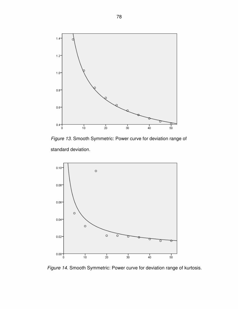
78

Figure 13. Smooth Symmetric: Power curve for deviation range of

standard deviation.

Figure 14. Smooth Symmetric: Power curve for deviation range of kurtosis.

79

Figure 15. Discrete Mass at Zero: Power curve for deviation range of

standard deviation.

Figure 16. Discrete Mass at Zero: Power curve for deviation range of

kurtosis.

80


standard deviation.


kurtosis.

81

Figure 19. Digit Preference: Power curve for deviation range of

standard deviation.

Figure 20. Digit Preference: Power curve for deviation range of kurtosis.

82

Figure 21. Multimodal Lumpy: Power curve for deviation range of

standard deviation.

Figure 22. Multimodal Lumpy: Power curve for deviation range of kurtosis.

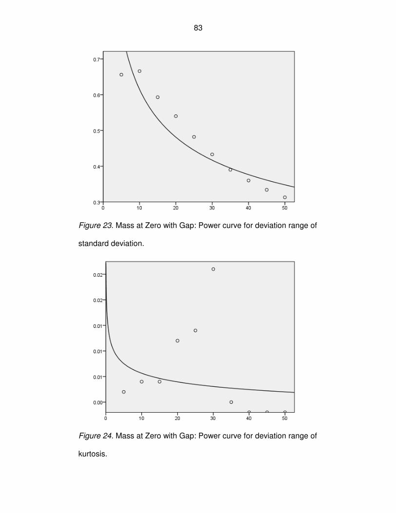
83

Figure 23. Mass at Zero with Gap: Power curve for deviation range of

standard deviation.


kurtosis.

84


standard deviation.


kurtosis.

85

Figure 27. Extreme Bimodal: Power curve for deviation range of standard

deviation.

Figure 28. Extreme Bimodal: Power curve for deviation range of kurtosis.

86

Power curves are variously selected for a second fitting with the addition of

the larger sample sizes. Figure 29 shows that inclusion of larger sample sizes

causes the Smooth Symmetric power curve to remain intact. This curve can be

compared with Figure 13. Figure 30 shows the rectifying of the Digit Preference

power curve fit when larger sample sizes are included. Compare this curve with

Figure 19. Figure 31 shows the Mass at Zero with Gap distribution, which achieves

an extremely poor fit when only small samples are included (see Figure 24), but

assumes the basic shape of the power curve with the addition of larger samples.

Together, these three large sample curves illustrate that to whatever extent

predictive patterns are established when n ≤ 50, those regression slopes either

improve in fit or continue to hold when sample sizes increase. Therefore, it does

not seem warranted to present a complete set of power curves with the larger

sample sizes.

87


deviation with inclusion of large sample sizes.

Figure 30. Digit Preference: Power curve for deviation range of standard

deviation with inclusion of large sample sizes.

88


kurtosis with inclusion of large sample sizes.

89

CHAPTER 5

CONCLUSION

The purpose of this study was to compare the accuracy of the Blom, Tukey,

Van der Waerden, and Rankit approximations in attaining the target moments of

the normal distribution. Means and standard deviations were scaled to the T to

facilitate interpretation in the context of standardized testing in education.

Accuracy was conceptualized in both relative and absolute terms, as expressed in

ranks and absolute values throughout the results tables. Deviation from target and

magnitude of deviation framed the comparison of accuracy measures.

A Monte Carlo simulation allowed the ranking methods’ performance to be

experimentally evaluated under a variety of real distributional conditions. Each

entry in the tables is the product of 10,000 iterations of a random selection

process. Replicating this experiment would produce slightly different numerical

values due to the random processes it involves. However, the design is sufficiently

powerful that the outcome of the comparisons would be identical.

The final two tables summarize the major findings according to moment,

sample size, and distribution. Table 34 presents the average deviation ranks and

values and Table 35 identifies the winning approximations by name. In Table 35,

hyphens ( - ) indicate that all values for the mean are zero. Forward slashes ( / )

indicate that three out of four values for skewness are tied.

90

Table 34

Deviation from Target, Summarized by Moment, Sample Size, and Distribution

Blom Tukey Van der

Waerden Rankit

Rank Value Rank Value Rank Value Rank Value Range

Moment

Mean 2.045 0.000 2.022 0.000 2.034 0.000 2.026 0.000 0.000

Standard Deviation 1.859 1.142 2.985 1.186 3.982 1.603 1.146 1.119 0.484

Skewness 2.668 0.192 2.477 0.192 2.269 0.191 2.586 0.192 0.001

Kurtosis 1.687 0.947 2.915 0.941 3.988 0.952 1.394 0.930 0.022

Sample Size

5 ≤ 50 1.976 0.609 2.585 0.628 3.103 0.769 1.720 0.603 0.166

100 ≤ 1000 2.231 0.435 2.599 0.423 2.962 0.447 1.883 0.416 0.031

Distribution

Smooth Symmetric 2.007 0.393 2.643 0.411 3.196 0.531 1.653 0.391 0.140

Discr Mass Zero 2.033 0.404 2.608 0.421 3.136 0.539 1.715 0.403 0.136

Asym – Growth 1.995 0.453 2.670 0.470 3.257 0.583 1.596 0.452 0.131

Digit Preference 2.039 0.390 2.622 0.408 3.131 0.527 1.692 0.370 0.158

Multimod Lumpy 1.987 0.412 2.624 0.396 3.126 0.510 1.737 0.376 0.134

Mass Zero w/Gap 2.239 1.129 2.465 1.126 2.747 1.204 2.103 1.113 0.092

Asym – Decay 2.238 0.726 2.528 0.739 2.765 0.835 2.046 0.725 0.109

Extreme Bimodal 1.980 0.655 2.649 0.669 3.190 0.765 1.753 0.654 0.112

91

Table 35

Winning Approximations, Summarized by Moment, Sample Size, and Distribution

1st Place 2nd Place 3rd Place 4th Place

Rank \ Value Rank \ Value Rank \ Value Rank \ Value

Moment

Mean T \ - V \ - R \ - B \ -

Standard Deviation R \ R B \ B T \ T V \ V

Skewness V \ V T \ B/T/R R \ B/T/R B \ B/T/R

Kurtosis R \ R B \ T T \ B V \ V

Sample Size

5 ≤ 50 R \ R B \ B T \ T V \ V

100 ≤ 1000 R \ R B \ T T \ B V \ V

Distribution

Achievement

Smooth Symmetric R \ R B \ B T \ T V \ V

Discrete Mass at Zero R \ R B \ B T \ T V \ V

Asymmetric – Growth R \ R B \ B T \ T V \ V

Digit Preference R \ R B \ B T \ T V \ V

Multimodal Lumpy R \ R B \ T T \ B V \ V

Psychometric

Mass at Zero with Gap R \ R B \ T T \ B V \ V

Asymmetric – Decay R \ R B \ B T \ T V \ V

Extreme Bimodal R \ R B \ B T \ T V \ V

92

Discussion

Moment 1—Mean

All four ranking methods attain the target value of 50 for the mean.

Differences appear in the numerical results only after the third decimal place, and

are therefore meaningless in terms of practical application. Most mean deviation

values are machine-constant zeros, meaning they are zero at least until the sixth

decimal place. Although these differences are reflected in the deviation and

magnitude ranks, they do not merit further summary statistics, such as deviation or

RMS range.

Moment 2—Standard Deviation

The absolute and relative accuracy of the four ranking methods in attaining

the target standard deviation differ substantially. Their average absolute deviation

from the target T score standard deviation is 1.263. This means that the

practitioner who uses any of the four ranking methods to normalize test scores

without reference to sample size or distribution can expect to obtain an estimated

standard deviation of 8.737 – 11.263. Adding the test instrument’s standard error

to this compounds the problem. An instrument with a standard error of three (± 3)

and a Z score of two would incur a final T score of 67.474 and 72.526, whose true

range would be between 64.474 and 75.526, for a total of 11.052. Even a standard

error half this size would lead to a true score range of 65.974 to 74.026, or 8.052.

Thus, a standard deviation that is off target by 1.263 would combine with a

standard error of ± 1.5 to nearly triple the size of the true score range, from a

theorized range of three to an actual range of more than eight. This is an increase

93

of 268%. As the standard error increases, the estimated difference between the

theorized and actual score range diminishes. At a standard error of three, this

increase is 184%. At a standard error of four, it becomes 163%.

The smallest observed deviation from the target standard deviation

occurred in the Multimodal Lumpy distribution, for which Rankit obtained an

average deviation value of 0.509. Van der Waerden’s method performed at its

worst in the Mass at Zero with Gap distribution, obtaining a 3.768 deviation value.

In applied terms, this means that a practitioner using Van der Waerden’s formula

for normalizing a standardized test score of Z = 2 could obtain a T score as low as

62.464 or as high as 77.536. Adding in a relatively modest standard error of two

and rounding to the nearest whole number, a test-taker’s strong performance could

result in an actual score as low as 60 or as high as 80. This range would indicate

that the test-taker’s true performance falls somewhere between the 74th

and the

99th

percentile. Such information would be useless for any real testing purpose. On

the other hand, the practitioner who uses Rankit with a Multimodal Lumpy

distribution (Z = 2) would obtain a T score between 68.982 and 71.018. Including a

standard error of two and rounding, the test-taker would see a final score of 67 to

73. A true score range of six is clearly preferable to a range of 20. However, even

the best ranking method produces an estimated half point deviation from the T

score’s target standard deviation. In one of the best applied scenarios, this means

that the true score range would still be 151% higher than the standardized test

instrument’s stated standard error.

94

When assessing the potential impact of selecting a ranking method on the

outcome of T scores, the average deviation score range (Table 34) may be

misleading. It indicates that the difference between the highest and the lowest

deviation values from the target standard deviation is less than a half point (0.484).

However, the gulf between the highest and lowest deviation values across all

distributions is vast: 3.259. By the same token, the average deviation range among

samples of 5 through 50 is 0.614, compared to 0.117 among samples of 100

through 1,000. Much more variability in the extent of ranking methods’ deviation

from target occurs among small samples than among large samples.

RMS values may provide additional insight here. As anticipated, the

magnitude of deviation from target as expressed in RMS values is highest for

samples of n = 5, with only one exception. The highest RMS for Extreme

Asymmetric – Decay is found at sample size 10. The highest RMS among all

sample sizes is 2.750, which is found at sample size 5 in the psychometric

distribution Mass at Zero with Gap. Four of the five achievement distributions attain

an RMS of zero at sample size 200. This lack of deviation magnitude holds for the

larger sample sizes as well. Among achievement distributions, only Extreme

Asymmetric – Growth does not attain a low RMS of zero. At sample size 200, it

reaches 0.003, which tapers off to 0.001 by n = 1,000. The average RMS range

among the five achievement distributions is 0.111 and among the three

psychometric distributions, 1.154. The average RMS range among all eight

distributions is 0.158, with most RMS variability found among the psychometric

distributions and the smaller samples. Curiously, all the worst RMS values belong

95

to Blom, yet Blom achieves second place in terms of relative and absolute

deviation from target (Table 35). This suggests that Blom’s approximation may

work by sacrificing some technical precision for reliability.

Moment 3—Skewness

The four ranking methods’ average deviation from the target skewness

value of the normal distribution is 0.192. The psychometric distribution Mass at

Zero with Gap contains the worst deviation value for skewness and the

achievement distribution Digit Preference contains the best. Blom and Tukey tie at

0.719 for the worst skewness performance in a given distribution, and Blom and

Rankit tie at 0.022 for the best. Ranking methods should not be selected on the

basis of their deviation from target skewness values because the deviation

quantities are small and the differences between them are negligible. Table 25

shows a three-way tie for second place between Blom, Tukey, and Rankit. Van der

Waerden scores its only first-place finish in this case, with a mere 0.001 margin of

win. Furthermore, it is not clear how deviations from normal skewness may affect

test scoring or interpretation.

Moment 4—Kurtosis

Kurtosis values show greater deviation from target than skewness values

but less than standard deviations. The average deviation value for kurtosis across

all sample sizes and distributions is 0.943. The average deviation is higher by

0.222 for the smaller samples (n ≤ 50) than for the larger sample sizes. Although

the difference between the highest deviation value on any distribution and the

lowest (1.145 on Extreme Bimodal and 0.328 on Mass at Zero with Gap,

96

respectively) appears substantial at 0.817, the overall difference between the best-

performing and worst-performing ranking methods is only 0.022 on kurtosis. RMS

values support the conclusion that differences on kurtosis are likely to have little

practical meaning. The psychometric distributions have higher RMS values than

the achievement distributions by an average of 0.176. The highest RMS value,

0.946, occurs at sample size 500 in the Mass at Zero with Gap distribution. The

third-highest RMS value, 0.726, occurs at sample size 15 in the Extreme Bimodal

distribution. The highest RMS value among achievement distributions, 0.556,

occurs at sample size 30 in the Extreme Asymmetric – Growth distribution.

However, all the lowest RMS scores on distributions occur at the smallest sample

size, n = 5. Aside from the question of how kurtosis considerations may actually

affect test scoring or interpretation, RMS values display irregularity and

nonconformity with the patterns established by the second and third moments.

Recommendations

The Blom, Tukey, Van der Waerden, and Rankit approximations display

considerable variability on the even moments, standard deviation and kurtosis.

Only standard deviation, however, has known practical implications for test scoring

and interpretation. Results for the odd moments, mean and skewness, may

contribute to the analytical pursuit of area estimation under the normal distribution.

The great variability between and within ranking methods on the standard

deviation suggests that practitioners should consider both sample size and

distribution when selecting a normalizing procedure.

97

Small samples and skewed distributions aggravate the inaccuracy of all

ranking methods. However, substantial differences between methods and

deviations from target are found among large samples and relatively symmetric

distributions as well. Therefore, scores from large samples should be plotted to

observe population variance, in addition to propensity scores, tail weight, modality,

and symmetry. Practitioners including analysts, educators, and administrators

should also be advised that most test scores are less accurate than they appear.

Caution should be exercised when making decisions based on standardized test

performance.

Table 35 simplifies this selection. Rankit is the most accurate method on the

standard deviation and on kurtosis when sample size and distribution are not taken

into account; it is the most accurate method among both small and large samples;

and it is the most accurate method among both achievement and psychometric

distributions. Van der Waerden’s approximation consistently performs the worst

across sample sizes and distributions. In most cases, Blom’s method comes in

second place and Tukey’s, third. The exceptions are trivial for applied purposes.

It would be useful to perform a more exhaustive empirical study of these

ranking methods to better describe their patterns. It would also be of theoretical

value to analyze the mathematical properties of their differences. More research

can be done in both theoretical and applied domains. However, for the purpose of

normalizing test scores in the social and behavioral sciences, these results suffice.

98

REFERENCES

Aiken, L. R. (1987). Formulas for equating ratings on different scales. Educational

and Psychological Measurement, 47(1): 51-54.

Aiken, L. R. (1994). Psychological Testing and Assessment, 8th

Ed. Boston: Allyn

and Bacon.

Allport, F. M. (1934). The J-curve hypothesis of conforming behavior. Journal of

Social Psychology, 5: 141-183.

American Educational Research Association (AERA), American Psychological

Association (APA), & National Council on Measurement in Education

(NCME) (1999). Standards for Educational and Psychological Testing.

Washington, D.C.: AERA.

Andrews, D. F., Bickel, P. J., Hampel, F. R., Huber, P. J., Rogers, W. H., & Tukey,

J. W. (1972). Robust estimates of location survey and advances. Princeton:

Princeton University Press.

Angoff, W. H. (1971). Scales, norms, and equivalent scores. In Thorndike, R. L.,

Ed. Educational Measurement, 2nd

Ed. Washington, D.C.: American Council

on Education.

—(1984). Scales, Norms, and Equivalent Scores. Princeton: Educational Testing

Service.

Bartlett, M. S. (1947). The use of transformations. Biometrics, 3(1): 39-52.

Retrieved August 6, 2007 from JSTOR database.

99

Blair, R. C. & Higgins, J. J. (1980). A comparison of the power of the Wilcoxon’s

rank-sum statistic to that of the Student’s t statistic under various non-

normal distributions. Journal of Educational Statistics, 5: 309-35.

Blair, R. C. & Higgins, J. J. (1985). Comparison of the power of the paired samples

t test to that of Wilcoxon’s signed-ranks test under various population

shapes. Psychological Bulletin, 97: 119-28.

Bliss, C. I., Greenwood, M. L., & White, E. S. (1956). A rankit analysis of paired

comparisons for measuring the effect of sprays on flavor. Biometrics, 12(4):

381-403. Retrieved March 26, 2007 from JSTOR database.

Blom, G. (1954). Transformation of the binomial, negative binomial, Poisson and

χ2 distributions. Biometrika, 41(3/4): 302-316.

Blom, G. (1958). Statistical Estimates and Transformed Beta-Variables. New York:

John Wiley & Sons.

Box, G. E. P. & Cox, D. R. (1964). An analysis of transformations. Journal of the

Royal Statistical Society, 26: 211-252.

Bradley, R. A. & Terry, M. E. (1952). Rank analysis of incomplete block designs I.

The method of paired comparisons. Biometrika, 39: 324-345.

Bradley, J. V. (1977). A common situation conducive to bizarre distribution shapes.

The American Statistician, 31: 147-150.

Bradley, J. V. (1978). Robustness? British Journal of Mathematical and Statistical

Psychology, 31: 144-152.

100

Brown, B. M. & Hettmansperger, T. P. (1996). Normal scores, normal plots, and

tests for normality. Journal of the American Statistical Association,

91(436):1668-1675. Retrieved August 6, 2007 from JSTOR database.

Cadwell, J. H. (1953). The distribution of quasi-ranges in samples from a normal

population. Annals of Mathematical Statistics, 24: 603-13.

Chang, S. W. (2006). Methods in scaling the basic competence test. Educational

and Psychological Measurement, 66: 907-929

Conover, W. J. (1980). Practical Nonparametric Statistics. New York: John Wiley &

Sons.

Cronbach, L. J. (1976). Essentials of Psychological Testing, 3rd

Ed. New York:

Harper & Row.

Davison, A. C. & Gigli, A. (1989). Deviance residuals and normal scores plots.

Biometrika, 76(2): 211-221. Retrieved August 3, 2007 from JSTOR

database.

Donaldson, T. S. (1968). Robustness of the F-Test to errors of both kinds and the

correlation between the numerator and the denominator of the F-ratio.

Journal of the American Statistical Association, 63: 660-676.

Dunn-Rankin, P. (1983). Scaling Methods. Hillsdale: Lawrence Erlbaum

Associates.

Federer, W. T. (1951). Evaluation of Variance Components from a Group of

Experiments with Multiple Classifications. Iowa Agricultural Experiment

Station Research Bulletin, 380.

101

Fisher, R. A. & Yates, F. (1938). Statistical Tables for Biological, Agricultural and

Medical Research. Edinburgh: Oliver and Boyd.

Fisher, R. A. & Yates, F. (1953). Statistical Tables for Biological, Agricultural and

Medical Research, 4th

Ed. London: Oliver and Boyd.

Friedman, M. (1937). The use of ranks to avoid the assumption of normality

implicit in the analysis of variance. Journal of the American Statistical

Association, 32(200): 675-701.

Galton, F. (1902). The most suitable proportion between the value of first and

second prizes. Biometrika, 1(4): 385-90.

Games, P. A. (1983). Curvilinear transformations of the dependent variable.

Psychological Bulletin, 93(2): 382-387.

Games, P. A. (1984). Data transformations, power, and skew: A rebuttal to Levine

and Dunlap. Psychological Bulletin, 95(2): 345-347.

Games, P. A. & Lucas, P. A. (1966). Power of the analysis of variance of

independent groups on non-normal and normally transformed data.

Educational and Psychological Measurement, 26: 311-327.

Glass, G. V., Peckham, P. D., Sanders, J. R. (1972). Consequences of failure to

meet the assumptions underlying the fixed effect analysis of variance and

covariance. Review of Educational Research, 42: 237-288.

Godwin, H. J. (1949). On the estimation of dispersion by linear systematic

statistics. Biometrika, 36: 92-100.

Gosset, W. S. (“Student”) (1908). The probable error of a mean. Biometrika, 6(1):

1-25.

102

Harter, H. L. (1959). The use of sample quasi-ranges in estimating population

standard deviation. Annals of Mathematical Statistics., 30: 980-99.

Harter, H. L. (1961). Expected values of normal order statistics. Biometrika,

48(1/2): 151-165. Retrieved August 3, 2007 from JSTOR database.

Hastings, C., Mosteller, F., Tukey, J. W., & Winsor, C. P. (1947). Low moments for

small samples: A comparative study of order statistics. Annals of

Mathematical Statistics, 18: 413-26.

Hinkle, D. E., Wiersma, W., & Jurs, S. G. (2003). Applied Statistics for the

Behavioral Sciences, 5th

Ed. Boston: Houghton Mifflin.

Hoaglin, D. C. (2003). John W. Tukey and data analysis. Statistical Science, 18(3):

311-318. Retrieved August 3, 2007 from JSTOR database.

Horst, P. (1931). Obtaining comparable scores from distributions of dissimilar

shape. Journal of the American Statistical Association, 26(176): 455-460.

Retrieved August 23, 2007 from JSTOR database.

Ipsen, J. & Jerne, N. (1944). Graphical evaluation of the distribution of small

experimental series. Acta Pathologica, Microbiologica et Immunologica

Scandinavica, 21: 343-361.

Irwin, J. O. (1925). The further theory of Francis Galton’s individual difference

problem. Biometrika, 17: 100-28.

Kendall, M. G. (1955). Further contributions to the theory of paired comparisons.

Biometrics, 11: 43-62.

Kendall, M. G. & Stuart, A. (1979). The Advanced Theory of Statistics, 4th

Ed., Vol.

2. New York: MacMillan.

103

Kline, P. (2000). Handbook of Psychological Testing, 2nd

Ed. London: Routledge.

Kolen, M. J. & Brennan, R. L. (2004). Test Equating, Scaling, and Linking:

Methods and practices, 2nd

Ed. New York: Springer Science+Business

Media.

Lehmann, E. L. (1975). Nonparametrics: Statistical Methods Based on Ranks. San

Francisco: Holden-Day.

Lester, P. E. & Bishop, L. K. (2000). Handbook of Tests and Measurement in

Education and the Social Sciences, 2nd

Ed. Lanham, MD: Scarecrow Press.

Levine, D. W. & Dunlap, W. P. (1982). Power of the F Test with skewed data:

Should one transform or not? Psychological Bulletin, 92(1): 272-280.

Levine, D. W. & Dunlap, W. P. (1983). Data transformation, power, and skew: A

rejoinder to Games. Psychological Bulletin,93(3): 596-599.

Levine, A., Liukkonen, J., & Levine, D. W. (1992). Predicting power changes under

transformations in ANOVA tests. Communications in Statistics, 21: 679-92.

McCall, W. A. (1939). Measurement. New York: MacMillan.

Mehrens, W. A. & Lehmann, I. J. (1980). Standardized Tests in Education, 3rd

Ed.

New York: Holt, Rinehart and Winston.

Mehrens, W. A. & Lehmann, I. J. (1987). Using Standardized Tests in Education,

4th

Ed. New York: Longman.

Micceri, T. (1989). The unicorn, the normal curve, and other improbable creatures.


Micceri, T. (1990). Proportions, pitfalls and pendulums. Educational and

Psychological Measurement, 50(4): 769-74.

104

Mosteller, F. (1951). Remarks on the method of paired comparisons: I. The least

squares solution assuming equal standard deviations and equal

correlations. Psychometrika, 16: 3-9.

Netemeyer, R. G., Bearden, W. O. & Sharma, S. (2003). Scaling Procedures:

Issues and Applications. Thousand Oaks: Sage Publications.

Nanna, M. J. & Sawilowsky, S. S. (1998). Analysis of Likert scale data in disability

and medical rehabilitation research. Psychological Methods, 3(1): 55-67.

Nunnally, J. C. (1978). Psychometric Theory. New York: McGraw-Hill.

Osborne, J. W. (2002). Normalizing data transformations. ERIC Digest,

ED470204. Available online: www.eric.ed.gov

Pearson, K. (1895). Contributions to the mathematical theory of evolution: II. Skew

variation in homogeneous material. Philosophical Transactions of the Royal

Society, Series A, 186: 343-414.

Pearson, K. (1902). Note on Francis Galton’s problem. Biometrika, 1(4): 390-9.

Pearson, K. & Hartley, H. O. (1954). Biometrika Tables for Statisticians, I.

Cambridge University Press for the Biometrika Trustees.

Pearson, K. & Pearson, M. (1931). On the mean character and variance of a

ranked individual, and on the mean and variance of the intervals between

ranked individuals. Biometrika, 23: 364-87.

Pearson, E. S. & Please, N. W. (1975). Relation between the shape of a

population distribution and the robustness of four simple test statistics.

Biometrika, 62: 223-241.

105

Pearson, E. S. & Tukey, J. W. (1965). Approximate means and standard

deviations based on distances between percentage points of frequency

curves. Biometrika, 52(3/4): 533-546. Retrieved August 6, 2007 from

JSTOR database.

Petersen, N. S., Kolen, M. J., & Hoover, H. D. (1989). Scaling, norming, and

equating. In R. L. Linn (Ed.), Educational Measurement, 3rd

Ed. New York:

American Council on Education; and Macmillan.

The Psychological Corporation (1955). Methods of expressing test scores. Test

Service Bulletin, 48: 7-10.

Sawilowsky, S., Blair, R. C., & Micceri, T. (1990). A PC FORTRAN subroutine

library of psychology and education data sets. Psychometrika, 55: 729.

Sawilowsky, S. & Blair, R. C. (1992). A more realistic look at the robustness and

Type II error properties of the t test to departures from population normality.


Sawilowsky, S. & Fahoome, G. (2003). Statistics Through Monte Carlo Simulation

with Fortran. Oak Park: JMASM.

Scheffé, H. (1952). An analysis of variance for paired comparisons. Journal of the

American Statistical Association, 47: 381-400.

Simon, H. A. (1955). On a class of skew distribution functions. Biometrika, 42: 425-

440.

Srivastava, A. B. L. (1959). Effect of non-normality on the power of the analysis of

variance test. Biometrika, 46: 114-122.

106

SPSS (2006). Statistical Package for the Social Sciences (SPSS) 15.0 for

Windows. Author.

Stigler, S. M. (1977). Do robust estimators work with real data? The Annals of

Statistics, 5(6): 1055-1098.

Student—See Gosset, W. S.

Tan, W. Y. (1982). Sampling distributions and robustness of t, F and variance-ratio

in two samples and ANOVA models with respect to departures from

normality. Communications in Statistics, A11: 2485-2511.

Tapia, R. A. & Thompson, J. R. (1978). Nonparametric Probability Density

Estimation. Baltimore: Johns Hopkins University Press.

Tarter, M.E. (2000). Statistical Curves and Parameters: Choosing an appropriate

approach. Natick: A K Peters.

Thissen, D. & Wainer, H. (2001). Test Scoring. Mahwah: Lawrence Erlbaum

Associates.

Thorndike, R. L. (1982). Applied Psychometrics. Boston: Houghton Mifflin.

Thurstone, L. L. (1928). Attitudes can be measured. The American Journal of

Sociology, 22(4): 529-554.

Tindal, G. (1987). The effect of different metrics on interpretations of change in

program evaluation. Remedial and Special Education, 8(5): 19-28.

Tippett, L. H. C. (1925). On the extreme individuals and the range of samples

taken from a normal population. Biometrika, 17: 364-87.

107

Tukey, J. W. (1957). On the comparative anatomy of transformations. The Annals

of Mathematical Statistics, 28(3): 602-632. Retrieved March 26, 2007 from

JSTOR database.

Tukey, J. W. (1962). The future of data analysis. The Annals of Mathematical

Statistics, 33(1): 1-67. Retrieved August 3, 2007 from JSTOR database.

Tukey, J. W. & McLaughlin, D. H. (1963). Less vulnerable confidence and

significance procedures for location based on a single sample:

Trimming/Winsorization. Indian Journal of Statistics, 25: 331-351.

Van der Waerden, B. L. (1952/1953a). Order tests for the two-sample problem and

their power. Proceedings Koninklijke Nederlandse Akademie van

Wetenschappen (A), 55 (Indagationes Mathematical 14): 453-458, & 56

(Indagationes Mathematicae 15): 303-316.

Van der Waerden, B. L. (1953b). Testing a distribution function. Proceedings

Koninklijke Nederlandse Akademie van Wetenschappen (A),56

(Indagationes Mathematicae 15): 201-207.

Visual Numerics (1994). IMSL Stat/Library: FORTRAN subroutines for statistical

applications, Vol. 1. Houston: Author.

Walker, H. M. & Lev, J. (1969). Elementary Statistical Methods, 3rd

Ed. New York:

Holt, Rinehart and Winston.

Wilks, S. S. (1948). Order statistics. Bulletin of the American Mathematical Society,

54: 6-50.

108

Wilson, E. B. & Hilferty, M. M. (1929). Note on C. S. Peirce’s experimental

discussion of the law of errors. Proceedings of the National Academy of

Science, 15: 120-125.

Wimberley, R. C. (1975). A program for the T-score normal standardizing

transformation. Educational and Psychological Measurement, 35: 693-695.

Wright, E. N. (1973). Examinations, marks, grades and scales: A working paper.

Ontario: Toronto Board of Education.

Zimmerman, D. W. & Zumbo, B. D. (2005). Can percentiles replace raw scores in

the statistical analysis of test data? Educational and Psychological

Measurement, 65: 613-638. Retrieved March 7, 2007 from

http://epm.sagepub.com

109

ABSTRACT

A COMPARISON OF RANKING METHODS FOR NORMALIZING SCORES

by

SHIRA R. SOLOMON

May 2008

Advisor: Shlomo S. Sawilowsky

Major: Evaluation and Research

Degree: Doctor of Philosophy

Normalizing transformations define the frame of reference for standardized

test score distributions, allowing for meaningful comparisons between tests.

Normalization equalizes the intervals between data points by approximating where

ordinal scores fall along a normal distribution and how much of the corresponding

area under the curve the ranked, cumulative proportions occupy. The most

prominent among such ranking methods are the Blom, Tukey, Van der Waerden,

and Rankit approximations. The purpose of this study was to provide an empirical

comparison of these ranking methods as they apply to standardized test scoring

and interpretation.

A series of Monte Carlo simulations was performed to compare their

accuracy in terms of achieving the T score’s specified mean and standard

deviation and unit normal skewness and kurtosis. Eight nonnormal distributions of

real achievement and psychometric data were used at 10 small and four large

sample sizes. All four ranking methods were found to be accurate on the odd

moments but displayed considerable deviation from target values on the even

110

moments. Standard deviation showed the most variability on both accuracy

measures: deviation from target and magnitude of deviation.

The substantial variability between and within ranking methods on the

standard deviation suggests that practitioners should consider both sample size

and distribution when selecting a normalizing procedure. However, Rankit is the

most accurate method among small and large samples, achievement and

psychometric distributions, and overall. Van der Waerden’s approximation

consistently performs the worst across sample sizes and distributions. These

results indicate that Rankit should be the default selection for score normalization

in the social and behavioral sciences.

111

AUTOBIOGRAPHICAL STATEMENT

SHIRA R. SOLOMON

Prior to her doctoral work in Educational Evaluation and Research at

Wayne State University, Shira Solomon received a Bachelor of Arts in

Comparative Literature from Columbia University (1994), a Bachelor of Arts in

Talmud and Rabbinic Literature from the Jewish Theological Seminary of America

(1994), and a Master of Science in Teaching from the New School for Social

Research (1997).

She has taught English Language Arts in New York City public schools,

English as a Foreign Language at National Taiwan University, English as a Second

Language at Wayne State University’s English Language Institute, and research

methods for allied health and human services at Madonna University and

University of Detroit – Mercy. She has also worked as a technical writer, a

communications writer, and an entertainment writer. She trained in social and

behavioral health research at the Institute of Gerontology and the School of

Medicine at Wayne State University.

Ms. Solomon’s research interests include assessment methodology and

the epidemiological investigation of literacy.

A COMPARISON OF RANKING METHODS FOR NORMALIZING SCORES ...

Documents

Transcript of A COMPARISON OF RANKING METHODS FOR NORMALIZING SCORES ...