A Comparison of Quantitative and Qualitative Hedge … Comparison of Quantitative and Qualitative...

A Comparison of Quantitative and Qualitative Hedge Funds

Ludwig Chincarini∗

May 26, 2010.

Preliminary Draft

Comments Welcome

Abstract

In the last 20 years, the amount of assets managed by quantitative and qualitative hedgefunds have grown dramatically. We examine the difference between quantitative and qualitativehedge funds in a variety of ways, including management differences and performance differences.We find that both quantitative and qualitative hedge funds have positive risk-adjusted returns.We also find that overall, quantitative hedge funds as a group have higher αs than qualitativehedge funds. The outperformance might be as high as 72 bps per year when considering all riskfactors. We also suggest that this additional performance may be due to better timing ability.

JEL Classification: G0, G10, G11, and G23

Key Words: quantitative portfolio management, alpha, hedge funds, returns

∗The author would like to thank Alex Nakao for dedicated research assistance, Jason Price, Mary Martin, andthe Claremont libraries for aid in acquiring the hedge fund data, Scott Esser for help with the data, Stephen Brown,David Hsieh, Bill Fung, and Neer Asherie for helpful comments, and Kristin McDonald for technical help. Contact:Ludwig Chincarini, CFA, Ph.D., is an assistant professor at the Department of Economics, Pomona College, 425N. College Avenue #211, Claremont, CA 91711. Email: [email protected]. Phone: 909-621-8881. Fax:909-621-8576.

I INTRODUCTION 1

I Introduction

In the last few years, quantitative portfolio management and quantitative equity portfolio manage-

ment in particular have been on the rise (see Figure 1). The growth in this method of investing can

be attributed to many factors, but perhaps four of them stand out. First, there has been an ad-

vancement in the education and tools for assessing financial markets quantitatively. Second, there

has been a dramatic improvement in the technology required to efficiently examine the markets

quantitatively. Third, there has been an increasing demand from pension funds and other large

institutional investors for an investment process. Quantitative investing lends itself more easily to

a more structured investment process. Fourth, some have argued that a quantitative disciplined

investment process might lead to superior returns than a qualitative investment process. In par-

ticular, Chincarini and Kim (2006) have discussed the potential advantages and disadvantages of

quantitative funds (Table 1) arguing that the advantages most likely outweigh the disadvantages.

[INSERT FIGURE 1 ABOUT HERE]

[INSERT TABLE 1 ABOUT HERE]

This paper is focused on addressing the last of these potential reasons for the growth in quan-

titative portfolio management. In particular, we attempt to study the performance characteristics

of quantitative and qualitative hedge funds. The advantages for quantitative funds include the

breadth of selections, the elimination of behavioral errors (which might be particularly important

during the financial crisis of 2008 - 2009), and the potential lower administration costs (after hedge

fund fees). The disadvantages for quantitative hedge funds include the reduced use of qualita-

tive types of data, the reliance on historical data, the ability to quickly react to new economic

paradigms. These three might have been especially crippling during the financial crisis of 2007 and

2009. Finally, there is the potential of data mining, which will lead to strategies that aren’t as

II DATA 2

effective once implemented. In this paper, we will only focus on the return differences rather than

attempting to detail which of the advantages or disadvantages in central in the return differences.

The paper is organized as follows: section II describes the hedge fund database used in this

study; section III discusses the differences between quantitative and qualitative hedge funds in

terms of fund characteristics, including fees, average age, investability, liquidity, transparency, and

legal structure; section IV discusses the performance models used to test for differences in ability

between quantitative and qualitative managers and presents those results; and section V concludes

the paper.

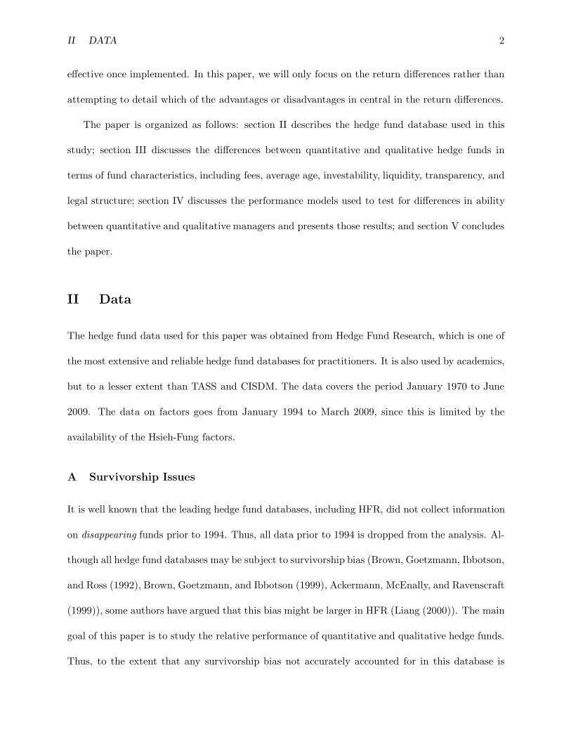
II Data

The hedge fund data used for this paper was obtained from Hedge Fund Research, which is one of

the most extensive and reliable hedge fund databases for practitioners. It is also used by academics,

but to a lesser extent than TASS and CISDM. The data covers the period January 1970 to June

2009. The data on factors goes from January 1994 to March 2009, since this is limited by the

availability of the Hsieh-Fung factors.

A Survivorship Issues

It is well known that the leading hedge fund databases, including HFR, did not collect information

on disappearing funds prior to 1994. Thus, all data prior to 1994 is dropped from the analysis. Al-

though all hedge fund databases may be subject to survivorship bias (Brown, Goetzmann, Ibbotson,

and Ross (1992), Brown, Goetzmann, and Ibbotson (1999), Ackermann, McEnally, and Ravenscraft

(1999)), some authors have argued that this bias might be larger in HFR (Liang (2000)). The main

goal of this paper is to study the relative performance of quantitative and qualitative hedge funds.

Thus, to the extent that any survivorship bias not accurately accounted for in this database is

II DATA 3

symmetric between funds, it should not alter the main purpose of this paper.

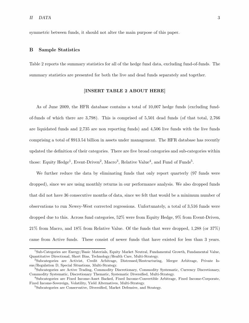
B Sample Statistics

Table 2 reports the summary statistics for all of the hedge fund data, excluding fund-of-funds. The

summary statistics are presented for both the live and dead funds separately and together.


As of June 2009, the HFR database contains a total of 10,007 hedge funds (excluding fund-

of-funds of which there are 3,798). This is comprised of 5,501 dead funds (of that total, 2,766

are liquidated funds and 2,735 are non reporting funds) and 4,506 live funds with the live funds

comprising a total of $913.54 billion in assets under management. The HFR database has recently

updated the definition of their categories. There are five broad categories and sub-categories within

those: Equity Hedge1, Event-Driven2, Macro3, Relative Value4, and Fund of Funds5.

We further reduce the data by eliminating funds that only report quarterly (97 funds were

dropped), since we are using monthly returns in our performance analysis. We also dropped funds

that did not have 36 consecutive months of data, since we felt that would be a minimum number of

observations to run Newey-West corrected regressions. Unfortunately, a total of 3,516 funds were

dropped due to this. Across fund categories, 52% were from Equity Hedge, 9% from Event-Driven,

21% from Macro, and 18% from Relative Value. Of the funds that were dropped, 1,288 (or 37%)

came from Active funds. These consist of newer funds that have existed for less than 3 years.

1Sub-Categories are Energy/Basic Materials, Equity Market Neutral, Fundamental Growth, Fundamental Value,Quantitative Directional, Short Bias, Technology/Health Care, Multi-Strategy.

2Subcategories are Activist, Credit Arbitrage, Distressed/Restructuring, Merger Arbitrage, Private Is-sue/Regulation D, Special Situations, Multi-Strategy.

3Subcategories are Active Trading, Commodity Discretionary, Commodity Systematic, Currency Discretionary,Commodity Systematic, Discretionary Thematic, Systematic Diversified, Multi-Strategy.

4Subcategories are Fixed Income-Asset Backed, Fixed Income-Convertible Arbitrage, Fixed Income-Corporate,Fixed Income-Sovereign, Volatility, Yield Alternatives, Multi-Strategy.

5Subcategories are Conservative, Diversified, Market Defensive, and Strategy.

II DATA 4

Another 1,190 (34%) came from liquidated funds and 1,038 (29%) came from non-reporting, but

existing funds. Finally, we drop funds for which the performance numbers are missing or they do

not have consecutive monthly return data (44 funds).6 This leaves a data set with a group of 6,353

hedge funds with about 53% from Equity Hedge, 10% from Event-Driven, 20% from Macro, and

17% from Relative Value. Finally, we drop all observations prior to 1994 given the aforementioned

issues with survivorship bias. The final data set consists of a total of 6,352 hedge funds.

C Classification of Quantitative and Qualitative Hedge Funds

We realize that most hedge are neither strictly quantitative (quant) or strictly qualitative (qual).

However, the goal of this paper is to make an attempt at sorting the two types of funds. Thus, if

the quantitative group of funds generally uses more quantitative investment techniques than the

qualitative group, we may learn about the relative importance of quantitative techniques.

In the hedge fund database, funds are classified according to their main strategy and their sub-

strategy. For each individual hedge fund, the database has a fund description. We use both of these

data sources to construct two classifications of quantitative and qualitative hedge funds.

C.1 Classification 1

For this classification method, we read all the hedge fund category descriptions and divided the

hedge funds according to Table 3.


Of all the hedge fund sub-categories we classified 10 as quantitative or qualitative and did not

categorize 18 of them as well as not including the fund-of-fund categories. Of the ones categorized,

6This can be for a variety of reasons. One of the most common reasons is that a fund begins reporting quarterly,but at a later date reports monthly. Thus, in the database, the fund is classified as a monthly reporter, even thoughfor a portion of its existence it was a quarterly reporter.

II DATA 5

we used either the strategy name and/or description to determine whether the funds were quantita-

tive or qualitative hedge funds7 Our main method used to classify each fund group was to look for

the term quantitative or a description of a similar nature to place a fund in the quantative category.

We also looked for words like discretionary to classify qualitative funds and systematic to classify

quantitative funds. Of the four main hedge fund categories, we only found two of them reliable

enough to classify. Thus, in the Equity Hedge category, we classified Equity Market Neutral and

Quantitative Directional as quantitative hedge funds and Fundamental Growth and Fundamental

Value as qualitative categories. In the Macro category, we classified Commodity Systematic, Cur-

rency Systematic, and Systematic Diversified as quantitative funds and Commodity Discretionary,

Currency Discretionary, and Diversified Thematic as qualitative funds. We did not classify any of

the Event Driven funds since these funds vary too substantially within the category and it was not

clear from the category descriptions how to separate quantitative and qualitative funds. We also

did not classify any of the Relative Value funds, even though many of these funds use quantitative

techniques, because the broader category descriptions left us no clear cut way to divide them. We

also left out a couple of Macro funds that could not be easily divided on category description alone.

C.2 Classification 2

In order to check our results against other methods of separating quantitative and qualitative hedge

funds, we considered all hedge funds again, but performed a word search on the strategy description

of each individual hedge fund in the database. We classified a fund as quantitative if the following

words appeared in the fund description: quantitative, mathematical, model, algorithm, econometric,

statistic, or automate. Also, the fund description could not contain the word qualitative. We

classified a fund as qualitative if it contained the word qualitative in its description or had none of

7The strategy descriptions are available directly from HFR (www.hedgefundresearch.com/) or from the authorsupon request.

III MANAGEMENT DIFFERENCES 6

the words mentioned for the quantitative category.

The bulk of the analysis in this paper is conducted with classification 1, however in the regression

analysis (the most important part of performance analysis in this paper), we present the results for

both classification method 1 and classification method 2.

III Management Differences

Table 4 produces some broad management characteristics about the quantitative and qualitative

hedge funds using classification 1. This information is from the most recent available information

in the database as of June 2009. First, there are many more non-quantitative hedge funds in our

study. This is both true as of June 2009 as well as on average across time (see the Avg. Number

column). Second, the average assets under management (AUM) over the entire time period is about

the same for quant and qual funds. We also created a measure of the growth in new assets over

the entire period for each hedge fund. We computed the average growth rate of new assets into

the average hedge fund using the formula for monthly growth in flows as: gt = New FlowstAUMt−1

, where

New Flowst = AUMt − AUMt−1 · (1 + rit), where rit is the net returns of fund i from t − 1 to t.

Using our measure, we find that on average across time and across funds, the average qualitative

fund has had an average growth in assets of 17% per month compared to quantitative funds of 11%.

Third, the average management fee does not differ too much, but is almost 25 bps higher for the

average quantitative fund. The average incentive fees 43 bps higher for qual funds. Fourth, of all

the quantitative funds, 82% have high water marks, while 92% of the qualitative funds have high

water marks.8 Quantitative funds have a slightly higher percentage of funds with hurdle rates.9

In the same table, we breakdown the statistics by hedge fund sub-strategy. The items of note are

8High water marks are defined by a “yes” or “no” in the database.9The database contains all sorts of hurdle rates, such as 6-month LIBOR or the 3-month Treasury bill rate, thus

we count the funds by looking at those that have no hurdle rate.

III MANAGEMENT DIFFERENCES 7

that Equity Market Neutral funds have had by far the largest AUM growth amongst quantitative

funds, while Fundamental Value and Currency Discretionary have had the highest AUM growth

for the qualitative category.


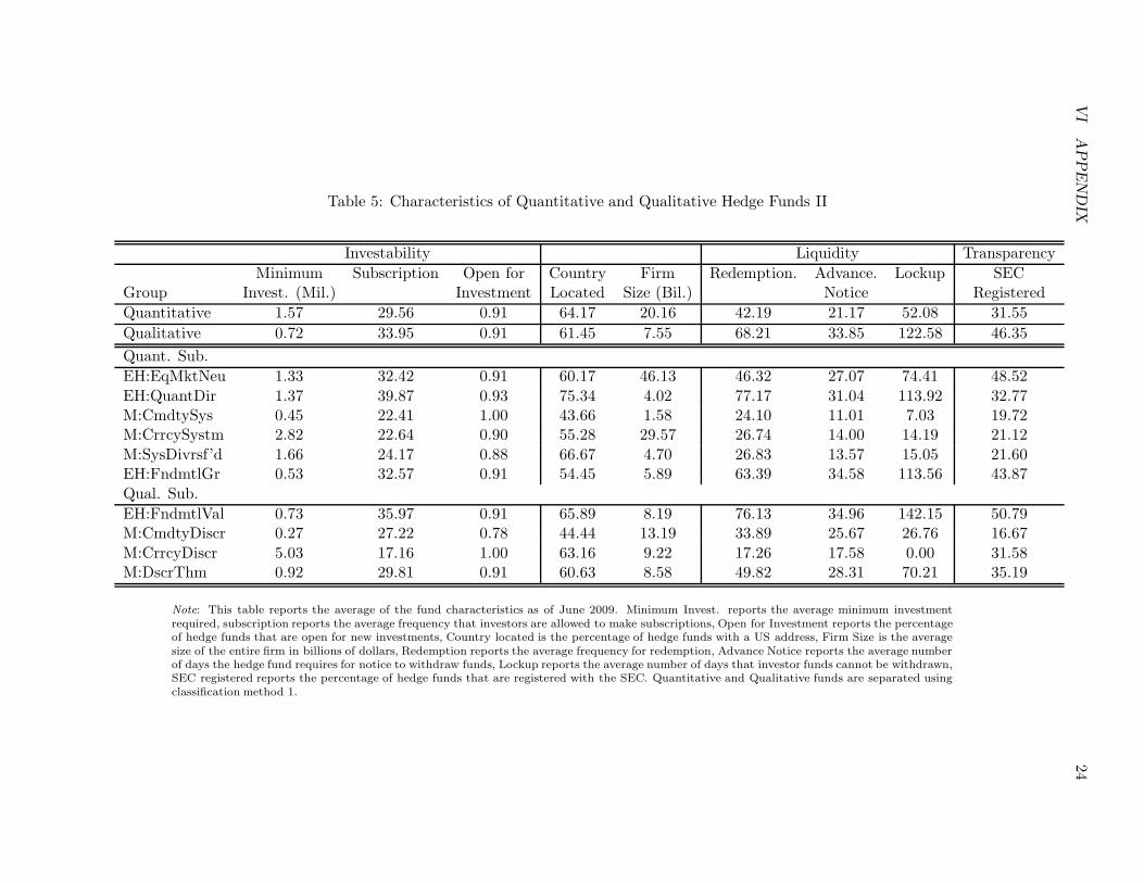
Table 5 contains other characteristics of these hedge fund categories. The average minimum

investment for quantitative funds is much higher than for qualitative funds ($1.57M versus $0.72M).

Both types of funds are generally open to new investments (91% of the funds), while they both

allow investors to make subscriptions roughly every four months (0.30% per year). About 64% and

61% of quantitative and qualitative funds have US addresses. The average firm size of quantitative

funds is substantially larger ($20B versus $8B). This might reflect the economies of scale inherent in

launching other quantitative hedge funds within the same firm with a similar quantitative process.

On the whole, qual funds look more illiquid, in the sense that the average redemption period is

longer, the amount of advanced notice a hedge funds needs for withdrawals is longer, and they have

on average almost double the lockup period (123 days versus 52 days).10 Quantitative hedge funds

seem to be less transparent on average than qual funds. In our sample, 32% are SEC registered

compared to 46% of the qual funds. This might be due to the sensitive nature of proprietary

models.


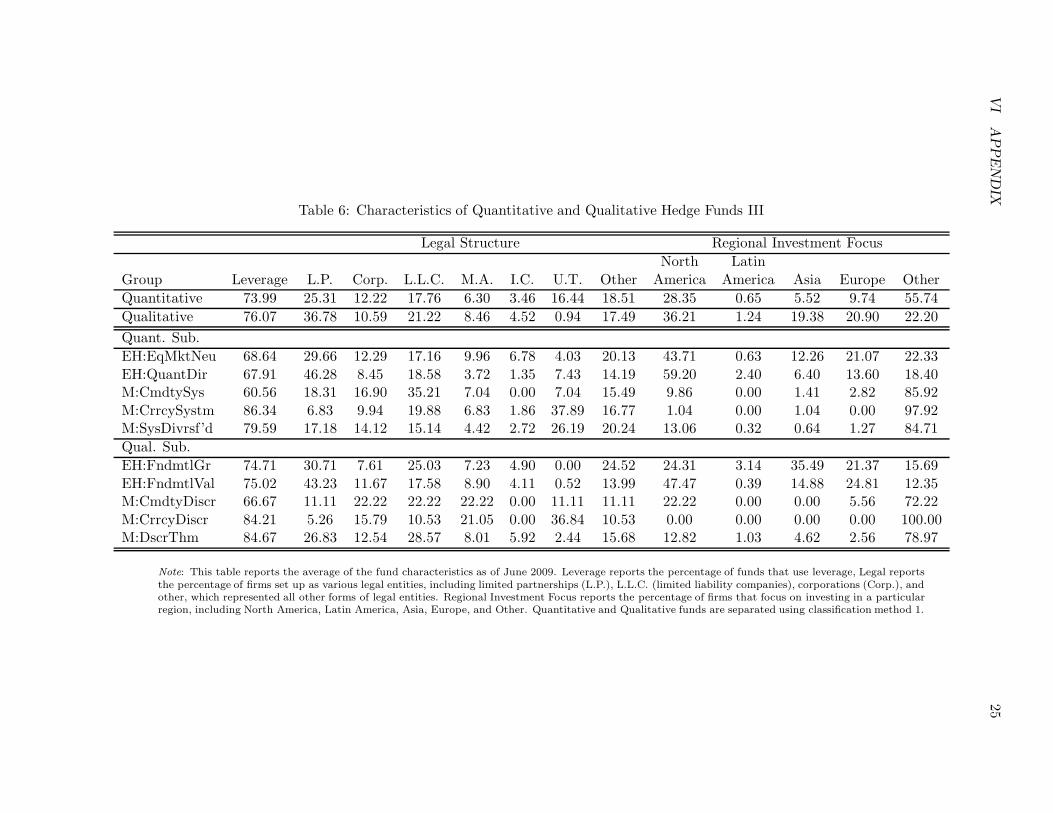
Table 6 is the final table that we present on the management differences between quant and

qual funds. The percentage of funds that use leverage is roughly equivalent at 74% and 76%.11

10The database contains various entries for subscription, including “Anytime”, ”Semi-Annual”, thus we convertedeach of these into a number of days. The same is true for redemptions, which are given values such as “1 year”,“Annually”, “18 Month”, etc. Thus we converted these into number of day equivalents as well. Lockup was alsogiven in text format, such as “1 Quarter”, “1 Day”, etc. and we converted these to a number of days format.

11There were various text responses to leverage in the database, including the specification of the amount ofleverage. We simply counted the ones that had an entry of no leverage.

IV PERFORMANCE DIFFERENCES 8

The types of legal structure are very similar, with limited partnerships (LP) and limited liability

companies (LLP) being the most common. On the whole, quant funds tend to invest less in North

America than qual funds. Macro Currency funds have almost zero investments in North America

both for qual and quant funds.12

Overall, despite some minor differences, the management characteristics of quant and qual funds

do not seem to be altogether different.


IV Performance Differences

In order to examine the performance differences of quantitative and qualitative hedge funds, we

must use performance metrics. In this paper, in addition to standard return and risk measures as

well as risk-adjusted measures, we also examine excess performance measures after acccounting for

some type of asset-pricing model.

The first set of models used are a standard CAPM and the Fama-French three-factor model.

Fung and Hsieh (2001, 2004) and Agarwal and Naik (2004) argue that the standard linear-factor

models, like the Fama-French model, may not be suitable for measuring the performance behavior

of hedge funds. This will be especially true for non-equity hedge funds. Thus, in addition to the

popular Fama-French model, we use a similar model to the one in Fung and Hsieh (2004). This

extended model contains the Fama-French market, size, value, and momentum factors. It also

contains the lookback straddles for bonds, foreign exchange, and commodities.13 The model also

12Not all funds reported for this category. Thus, amongst the funds that had a response we computed the percent-ages invested in various regions. Europe contained several categories, including Northern Europe, Pan-European,Russia/Eastern Europe, Western Europe/UK. Asia contained several categories including Asia ex-Japan, Asia w/Japan, and Japan. The Other category included Pan-American, Africa, Global, Middle East, and Multiple EmergingMarkets.

13The lookback straddle data was obtained from http://faculty.fuqua.duke.edu/ dah7/DataLibrary/TF-FAC.xls.


contains two bond related factors. The first is the Lehman US 10-year bellwether total return

index. The second is the total return difference between the Lehman US aggregate intermediate

BAA corporate index and the 10-year bellwether index. Finally, we include an emerging market

equity index.

Thus, the models estimated are the following:

r̃it = αiT + β1iTRMRF + εit t = 1, 2, ...T (1)

r̃it = αiT + β1iTRMRF + β2iTSMB + β3iTHML + εit t = 1, 2, ...T (2)

r̃it = αiT + β1iTRMRF + β2iTSMB + β3iTHML + β4iTMOM (3)

+ β5iT10yr + β6iTCS + β7iTBdOpt + β8iTFXOpt

+ β9iTComOpt + β10iTEE + εit t = 1, 2, ...T

where r̃it(= rit−rft) is the net-of-fee return on a hedge fund portfolio in excess of the risk-free rate,

RMRF is the excess return on a value-weighted aggregate market proxy, SMB, HML, and MOM

are the returns on a value-weighted, zero-investment, factor-mimicking portfolios for size, book-

to-market equity, and one-year momentum in stock returns as computed by Fama and French,14

10yr is the Lehman US 10-year bellwether total return, CS is the Lehman aggregate intermediate

BAA corporate bond index return minus the Lehman 10-year bond return, BdOpt is the lookback

straddle for bonds, FXOpt is the lookback straddle for foreign exchange, ComOpt is the lookback

straddle for commodities, and EE is the total return from an emerging market equity index. These

models are typically employed to extract the stock picking skill of the portfolio manager or has

Henrikson and Merton like to call security analysis or the microforecasting ability of the portfolio

manager.

For the tests of market timing, the above models have been modified to include a term that

The lookback straddle is a derivative security that pays the holder the difference of the maximum and minimumprices of the underlying asset over a given time period. For more information on the calculation of these straddles,please see Fund and Hsieh (2004).

14Source: http://mba.tuck.dartmouth.edu/pages/faculty/ken.french/data library.html.


captures the market timing ability (or macroforecasting skills) of the portfolio manager.

r̃it = αiT + β1iTRMRF + γiTTIMING + εit t = 1, 2, ...T (4)

r̃it = αiT + β1iTRMRF + β2iTSMB + β3iTHML + γiT TIMING + εit t = 1, 2, ...T (5)

r̃it = αiT + β1iTRMRF + β2iTSMB + β3iTHML + β4iTMOM (6)

+ β5iT10yr + β6iTCS + β7iTBdOpt + β8iTFXOpt

+ β9iTComOpt + β10iTEE + γiTTIMING + εit t = 1, 2, ...T

where TIMING is the standard measure of market timing, max(0,−[rM,t−rf,t]) (Henrikson-Merton

(1981). Focusing on the first equation, which is a standard CAPM test with a TIMING variable,

a perfect market timer should have a β = 1 and a γ = 1. This would imply an equity portfolio

manager that is 100% invested in equities, however in any month where the return of the market

is less than the risk-free rate, the manager will sell the entire portfolio and put the securities in

cash.15 In reality, it will be rare for hedge fund managers to engage in such an extreme market

timing procedure, however Merton (1981) shows that as long as the timer has greater than random

accuracy in predicting up and down markets and that he alters beta accordingly in up and down

markets, then γ will be positive and significant. Thus, a test for a positive and significant γ is

sufficient to find market timing ability. All of our measurement periods of performance are from

January 1994 - March 2009 unless otherwise indicated.

A Raw Performance

Table 7 shows performance summary statistics for the quantitative and qualitative funds using

classification method 1. Generally, quantitative funds have a higher average return and a lower

average standard deviation than qual funds. Amongst the quant funds, the highest average return

comes from the Quantitative Directional strategy. The correlations of the fund categories with the

15In theory, the portfolio manager does not need to liquidate the entire portfolio, they could simply engage in aposition that effectively changes the β from 1 to 0.


S&P 500 are quite low at 0.17 and 0.38 for quant and qual respectively. The risk-adjusted return

measures provide mixed evidence, but overall seems in favor of quant funds. The average Sharpe

and Omega ratio are higher for the qual category, while the Sortino, Calmar, and Sterling ratios

are higher for the quant category.

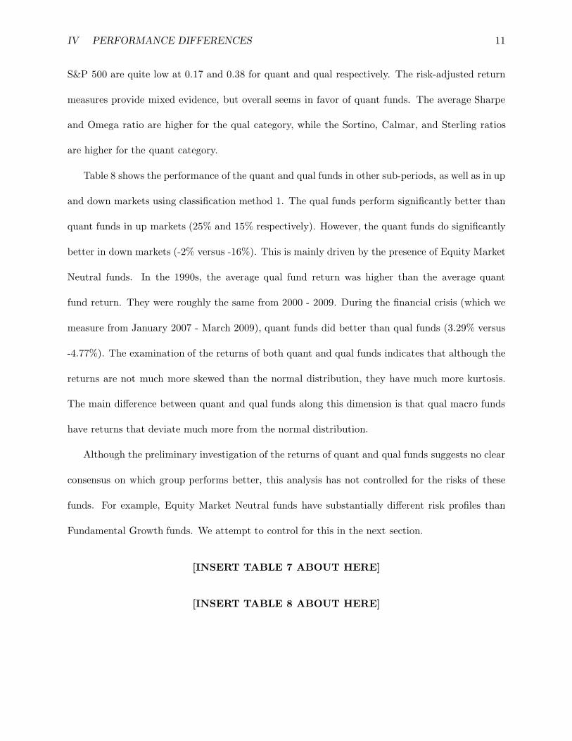
Table 8 shows the performance of the quant and qual funds in other sub-periods, as well as in up

and down markets using classification method 1. The qual funds perform significantly better than

quant funds in up markets (25% and 15% respectively). However, the quant funds do significantly

better in down markets (-2% versus -16%). This is mainly driven by the presence of Equity Market

Neutral funds. In the 1990s, the average qual fund return was higher than the average quant

fund return. They were roughly the same from 2000 - 2009. During the financial crisis (which we

measure from January 2007 - March 2009), quant funds did better than qual funds (3.29% versus

-4.77%). The examination of the returns of both quant and qual funds indicates that although the

returns are not much more skewed than the normal distribution, they have much more kurtosis.

The main difference between quant and qual funds along this dimension is that qual macro funds

have returns that deviate much more from the normal distribution.

Although the preliminary investigation of the returns of quant and qual funds suggests no clear

consensus on which group performs better, this analysis has not controlled for the risks of these

funds. For example, Equity Market Neutral funds have substantially different risk profiles than

Fundamental Growth funds. We attempt to control for this in the next section.




B Risk-Adjusted Performance

In this section, we analyze the performance of quantitative and qualitative funds using both clas-

sification methods 1 and 2. Table 9 contains the risk-adjusted return measures from the models

discussed earlier in Section IV. Columns (1) - (10) contain the results using classification method 1

to separate quantitative and qualitative hedge funds. Columns (1) - (4) represent panel regressions

on quant funds using a CAPM model, a three-factor Fama-French model, and a 10-factor Fama-

French model with Hsieg-Fund factors and emerging equities (henceforth denoted as the 10-factor

model), and the 10-factor model controlling for fixed sub-strategy effects and yearly time effects.

Columns (5) - (8) do the same but for a panel of qualitative funds. Columns (9) - (12) run panel

regressions including both quant and qual funds with a 10-factor model with (Column (10)) and

without (Column (9)) interaction dummies on the parameters.

Columns (11) - (16) contain results for classification method 2 (fund description classifications)

of quant and qual funds. Since the categorization in classification 2 was done by fund description,

this allows us to consider quantitative and qualitative funds within a particular fund category. We

do it for the four main hedge fund categories, Equity Hedge, Macro, Event Driven, and Relative

Value. Columns (11) and (12) presents the 10-factor model with and without interaction dummies.

Column (13) presents the 10-factor model results for quant and qual divided within the Equity

Hedge category. Column (14) presents the 10-factor model results for quant and qual divided

within the Macro category. Column (15) presents the 10-factor model results for quant and qual

divided within the Event Driven category. Column (16) presents the 10-factor model results for

quant and qual divided within the Relative Value category. In all cases, a dummy for quant funds

is included in the regressions with coefficient δ.



Columns (1) - (3) indicate that quant funds have large and significant αs even when using a

10-factor model. Column (3) reports an α of 0.32 which is equivalent to 0.32% per month or 3.84%

per year. The qual funds also have positive and significant αs, although generally smaller than the

quant funds.

Columns (9) - (12) report the pooled regressions. The important coefficient is the coefficient

on δ which reports the amount to add or subtract from α to get the true α of quant funds versus

qual funds. In Column (9), the δ̂ is negative, however, we did not control for the fact that quant

and qual funds most likely have very different factor exposures. In Column (10), we control for

this factor exposure difference and find that the δ̂ is indeed positive and significant. In fact, in this

specification, we find that the α is 0.26%, with δ = 0.06. Thus, quant funds have an α that is 6 bps

higher per month than qual funds after accounting for fees. This result is similar when the quant

and qual funds are divided according to words in their fund description (see Column (12)).

The results hold within main hedge fund categories where quant and qual are separated within

each category by their fund descriptions. For all categories, the δ̂ is positive and it is statistically

significant for the Macro and Relative Value categories.

As a further look into the issue, we performed the same analysis on equal-weighted composites

of each category. That is, every month, we took all the hedge funds that were quant funds and

took the equal-weighted average of their returns and created a monthly index for quant fund

performance. We did a similar thing for qual funds and sub-strategies. We then took these indices

and investigated the same performance issues. These results are produced in Table 10.


The results are qualitatively very similar. The quant index has a positive and significant α̂

that is higher than the α̂ of the qual funds. The α̂ in the 10-factor pooled regressions is 0.35% per


month and the δ̂ is 0.10% per month. Thus, for the index composites the quant funds have higher

risk-adjusted performance, but it is not as strong as the individual hedge fund regression results.

In order to examine this issue from yet another perspective, rather than using pooled regressions,

we run regressions on each individual hedge fund in each category and then average the coefficient

estimates, as well as compute the average of the t-statistics, and the percentage of funds in each

category that recorded a positive and significant value for that coefficient.16 For each category,

the number of funds used to compute the average coefficients is presented as N . The results are

produced in Table 11.


The results are presented for two of the performance models; the CAPM model and the 10-

factor model. Focusing on the quant category, we find that the average α̂s are all positive and

significant. For the 10-factor model, 18% of the quant funds have a positive and significant α̂. The

average α̂ for the quant funds is greater than the average α for the qual funds.

The evidence presented for our hedge fund sample over the period 1994-2009 suggests that

quant funds as a group outperformed qual funds on a risk-adjusted basis.

C Market Timing

In this section, we investigate the difference in market timing ability between quant and qual funds.

We implement the same regressions as before with a Henrikkson-Merton timing variable included

16The reader should note that the average t-statistics does not tell us anything about the average coefficient’ssignificance. In fact, a more appropriate measure for the average coefficient’s significance is to construct the statistics“average” t-statistic assuming that the coefficients of each fund are uncorrelated. If we are interested in the statistic,¯̂x = 1

N

PNi=1 x̂, then assuming normality from the central limit theorem and independence across parameter estimates,

we can use s¯̂x = 1N

q

PNi=1 s2

ix̂, where N is the number of hedge funds used in the average. The “average” t-statistic

or the t-statistic of the average of the parameter across the hedge funds is given by t-stat =¯̂x

s ¯̂x. While the assumption

of independence may not necessarily be true, it isn’t any worse than computing the average t-statistic, which is notreally interpretable. Although not reported, these t-statistics are very high. These statistics are available from theauthors upon request.


as discussed earlier in Section IV. The results are presented in Table 12. Columns (1) - (4) show

a positive and significant timing coefficient (γ̂ > 0) for the quant hedge funds. The α̂ of the 10-

factor model is negative for both quant and qual hedge funds. The qual funds also have positive

and significant timing coefficients for the 10-factor model, but not for the CAPM or three-factor

Fama-French model (see Columns (5) - (8)). Columns (9) - (12) present the pooled regression

results of quant and qual hedge funds with a timing variable included. The interaction dummy on

the timing variable shows decisively that the pooled timing coefficient for hedge funds is positive

(β̂T iming > 0) and that quant funds are better at timing (β̂Quant×T iming > 0) in both cases. For

the main quant-qual definitions (Column (10)), it is 0.08 per month and for the text division of

quant-qual (Column (12)) it is 0.09 per month.17


Another very interesting result is that when the timing variable is included in the pooled

regressions, the coefficient of δ̂ becomes negative and significant (ranging from -0.09% to -0.12%).

This evidence seems to suggest that on average quant funds’ excess performance over qual funds

comes from the quant hedge funds’ ability to engage in market timing of some sort. It should be

noted that significance of the market timing variable may be due to the timing of other factors in

their quantitative models but is being picked up by the market timing proxy.

D The Financial Crisis of 2007-2009

In this section we compare the performance of quant and qual funds during the financial crisis of

2008. Although the exact dates of the financial crisis may vary by one’s perspective, we chose a

period that gave us sufficient observations and encapsulated the crisis. Some observers noted that

17To get the actual impact on performance, one would have to multiply this estimate times the average value ofthe quant timing variable.


the worst month of the financial crisis for quant funds was August 2007. Clearly, other times in

2008 were more devastating to the overall markets, including the near failure of Bear Stearns in

March 2008 and the collapse of Lehman Brothers in September 2008. In order to capture enough

data and all of these events, we used the period January 2007 - March 2009 as our measurement

period. Table 13 contains the results of the analysis over this period. Generally, quant funds have

positive αs over the crisis period. The α̂s are also statistically significant except for the 10-factor

specification. Qual funds do worse than quant funds, having a significantly negative α̂ except for

the CAPM specification.

Columns (9) - (12) show that the δ̂s are all positive and signficant indicating that the quant

hedge funds had a significantly higher α during the crisis. The δ̂ estimates range from as little as

22 bps per month to as much as 45 bps per month. The evidence for the quant versus qual within

categories suggests the same. The δ̂s are all positive and significant for the Macro category.


E The Composition of Deciles

In this section, we examine the performance of quant and qual hedge funds by their decile rankings

using classification method 1. We look at their relative performance in three ways. First, we

examine the raw returns of both quantitative and qualitative hedge funds. Second, we investigate

the risk-adjusted returns using the three-factor α, and third, we use the risk-adjusted returns using

the 10-factor α. For various time periods, we sort the performance of these hedge funds from

highest to lowest and then compute the percentage of quantitative hedge funds in each decile for

the period. Only hedge funds that exist at the beginning and ending of any period are used in the

analysis. For each period, hedge fund returns are ranked from highest to lowest. They are divided

into deciles. n1 is the number of quantitative funds used in the analysis for the particular period,

V CONCLUSION 17

n2 is the number of qualitative funds used in the analysis for the particular period. Decile 1 contain

the funds with the lowest returns or α, while Decile 10 contain the funds with the highest returns or

α. For each performance period, the percentage of quantitative funds in each decile as a percentage

of the total number of quantitative funds is computed. Similarly, the percentage of qualitative

funds in each decile as a percentage of total qualitative funds is computed. The table reports the

difference between the quantitative and qualitative percentage in each decile. The sum of this over

all deciles should equal 0. We report those percentages in Table 14. The table also contains the

sum of the values of deciles 9 and 10 minus the value of deciles 1 and 2. A positive value of this

metric indicates that on average more quant funds are in the higher performance deciles relative to

qual funds.

The raw returns contain mixed evidence. For example, from 1994-2000, this value is 17.63,

while from 2000-2009 it is -19.09. The three-factor Fama-French αs are more consistent with quant

funds outperforming qual funds. The values are higher and positive except for the main part of the

period. The 10-factor Fama-French αs is the most consistent with quant funds outperforming qual

funds.


V Conclusion

The growth of hedge funds over the last 20 years has been enormous. There has been a literature to

determine whether hedge funds can perform well on a risk-adjusted basis, since they tend to attract

talented people, have less investing restrictions, and have higher incentives. Within the hedge fund

world, two camps of management have also grown; the traditional qualitative or fundamental camp

and the quantitative camp. This paper takes a first look at the different types of hedge fund

V CONCLUSION 18

managing styles. Quantitative and qualitative hedge funds are examined in a variety of ways,

including their management differences and their performance differences. The paper finds that

management differences among quantitative and qualitative hedge funds are few. First, there are

many more qualitative funds with less average assets under management. Second, the average

quant hedge fund has a larger firm size. Third, the average quant hedge fund has more liquidity

for investors. Fourth, the average percent of quantitative hedge funds registered with the SEC is

less than the average number of qualitative funds.

Performance differences, although not large, seem to exist. We use two classification methods

to separate quantitative and qualitative hedge funds and find the results are similar using both

methods. Generally, quant funds perform better than qualitative funds using a variety of risk-

adjusted performance metrics. Quantitative funds also seem to be better market timers than qual

funds. In fact, it may be precisely the market timing that allows them to outperform the qual

funds.

Hedge funds use quantitative techniques to varying degrees. Our separation of hedge funds into

quantitative and qualitative is an initial attempt to capture any differences in performance due

to quantitative investment techniques. Future research should investigate the sensitivity of these

results to other definitions.

VI APPENDIX 19

VI Appendix

VI APPENDIX 20

A Tables

Table 1: The Advantages and Disadvantages of Quantitative versus Qualitative Management

Advantages

Criteria QEPM Qualitative

Objectivity High Low

Breadth High LowBehavioral Errors Low High

Replicability High LowCosts Low High

Controlled Risk High Low

Disadvantages

Criteria QEPM Qualitative

Qualitative Inputs Low HighHistorical Data Reliance High Low

Data Mining High LowReactivity Low High

Note: Source: Chincarini and Kim (2006).

VI APPENDIX 21

Table 2: Hedge Fund Database Summary Statistics

Total Avg. Avg. Avg. Avg. Avg. Avg. High Water Hurdle RateGroup Number Number AUM Growth M. Fee I. Fee Age (%) (%)

Equity Hedge 3348 1413.73 102.62 0.15 1.34 18.91 6.92 89.67 13.71EH:Engy/Bmat 134 47.56 88.27 0.04 1.45 20.13 5.80 91.79 10.45EH:EqMktNeu 472 188.17 111.59 0.20 1.35 19.46 6.50 87.50 22.67EH:FndmtlGr 775 337.97 90.95 0.05 1.39 18.44 7.11 87.35 16.65EH:FndmtlVal 1337 581.72 112.64 0.26 1.32 19.47 6.99 94.02 9.80EH:QuantDir 296 117.63 142.36 0.05 1.28 16.16 7.35 76.01 15.54EH:Short Bias 43 21.07 25.24 0.05 1.23 18.40 8.98 81.40 4.65EH:Tech/Hlth 235 94.72 59.75 0.03 1.33 19.56 6.43 93.19 10.21EH:MultStrat 56 24.90 33.43 0.05 1.14 19.29 7.08 94.64 10.71

Event-Driven 622 285.19 163.46 0.05 1.46 19.67 7.54 95.02 7.72ED:Activist 23 9.66 194.02 0.04 1.72 20.00 6.62 100.00 8.70ED:CreditArb 23 7.50 132.51 0.04 1.56 20.00 5.15 100.00 4.35ED:Dstrd/Rstrc 180 84.97 171.71 0.03 1.46 19.03 7.75 95.00 6.67ED:MergerArb 91 48.74 109.54 0.02 1.26 19.40 8.68 92.31 9.89ED:PvIss/RegD 38 14.89 70.12 0.04 1.70 20.58 5.59 97.37 2.63ED:SpecialSit 257 113.92 164.85 0.08 1.47 19.92 7.36 95.33 8.17ED:Mult-Strat 10 6.66 582.65 0.02 1.83 24.43 12.73 80.00 20.00Macro 1263 542.34 129.75 0.12 1.88 19.15 7.33 84.88 9.58

M:ActiveTrd 29 12.16 154.47 0.07 3.00 20.00 6.91 100.00 3.45M:CmdtyDiscr 18 7.71 45.71 0.06 1.75 20.00 6.38 66.67 5.56M:CmdtySys 71 30.78 61.65 0.04 1.37 12.21 7.09 74.65 19.72M:CrrcyDiscr 19 9.32 104.35 0.25 2.00 20.00 7.93 89.47 10.53M:CrrcySystm 161 68.58 221.59 0.06 1.80 20.19 7.41 82.61 8.70M:DscrThm 287 115.50 154.63 0.11 1.66 18.95 6.66 95.47 11.50M:SysDivrsf’d 588 261.02 103.49 0.10 2.06 19.30 7.80 80.10 5.95M:Mult-Strat 90 37.69 190.72 0.35 1.57 20.00 6.68 92.22 23.33Relative Val 1119 459.21 155.51 0.06 1.37 18.60 6.67 84.18 17.43

RV:FI-AsstBkd 135 58.47 146.28 0.08 1.23 18.78 6.84 85.19 22.96RV:FI-CnvArb 210 100.96 116.08 0.03 1.33 18.24 7.94 82.86 14.76RV:FI-Corp 213 80.65 203.97 0.04 1.32 17.98 6.32 81.69 16.43RV:FI-Sovergn 37 14.54 137.84 0.05 1.29 20.00 6.27 81.08 37.84RV:Volatility 81 27.51 45.47 0.05 1.59 20.00 5.35 93.83 2.47RV:YieldAlt 53 17.52 44.17 0.07 1.27 18.33 5.26 77.36 22.64RV:Mult-Strat 390 159.56 191.50 0.08 1.45 18.92 6.63 85.13 17.95

Live Funds 3198 1476.05 146.17 0.14 1.52 19.24 7.43 91.59 12.66Dead Funds 3154 1224.43 87.91 0.09 1.45 18.94 6.60 84.91 13.25All 6352 2700.48 123.86 0.12 1.46 18.97 7.02 88.27 12.96

Note: This table reports the time-series averages of annual cross-sectional averages from January 1994 - March 2009.Avg. Number is the average number of hedge funds across monthly observations, Avg. AUM represents the averageassets under management across months, Avg. Growth computes the average growth rate of new assets into the

average hedge fund using the formula for monthly growth in flows as: gt = New Flowst

AUMt−1

, where New Flowst =

AUMt − AUMt−1 · (1 + rit), where rit is the net returns of fund i from t − 1 to t, Avg. M. Fee is the averagemanagement fee across hedge funds, Avg. I. Fee is the average incentive fee across hedge funds, Avg. Age is theaverage number of years of existence of a fund in a particular category, High Water (%) is the percentage of hedgefunds in the database with a high water mark across funds and time, and Hurdle Rate (%) is the percentage of fundswith a hurdle rate across funds and time.

VI APPENDIX 22

Table 3: Classification 1 of Quantitative and Qualitative Funds

Categorized

Quantitative Qualitative

Number Main Sub Sub

1. Equity Hedge

EH: Equity Market Neutral EH: Fundamental GrowthEH: Quantitative Directional EH: Fundamental Value

2. Macro

M: Commodity Systematic M: Commodity DiscretionaryM: Currency Systematic M: Currency Discretionary

M: Systematic Diversified M: Discretionary Thematic

Uncategorized

1. Equity HedgeEH: Energy/Basic Materials EH: Short-Biased

EH: Technology/Healthcare EH: Multi-Strategy

2. Event-DrivenED: Activist ED: Credit Arbitrage

ED: Distressed/Restructuring ED: Merger ArbitrageED: Private Issue/Regulation D ED: Special Situations

3. Macro

M: Active Trading M: Multi-Strategy

4. Relative ValueRV: Fixed Income-Asset Backed RV: Fixed-Income-Convertible Arbitrage

RV: Fixed Income-Corporate RV: Fixed Income-SovereignRV: Volatility RV: Yield Alternative

RV: Multi-Strategies

5. Fund of FundsFOF: Conservative FOF: Diversified

FOF: Diversified FOF: Market DefensiveFOF: Strategic

Note: Source: HFR strategy descriptions and authors’ judgement. For a full description of each fund main categoryand sub-category, see the appendix.

VI APPENDIX 23

Table 4: Characteristics of Quantitative and Qualitative Hedge Funds I

Total Avg. Avg. Avg. Avg. Avg. Avg. High Water Hurdle RateGroup Number Number AUM Growth M. Fee I. Fee Age (%) (%)

Quantitative 1588 666.18 119.85 0.11 1.64 18.65 7.26 81.55 13.60

Qualitative 2436 1051.79 110.46 0.17 1.39 19.08 6.99 91.83 12.15

Quant. Sub.

EH:EqMktNeu 472 188.17 111.59 0.20 1.35 19.46 6.50 87.50 22.67EH:QuantDir 296 117.63 142.36 0.05 1.28 16.16 7.35 76.01 15.54M:CmdtySys 71 30.78 61.65 0.04 1.37 12.21 7.09 74.65 19.72M:CrrcySystm 161 68.58 221.59 0.06 1.80 20.19 7.41 82.61 8.70M:SysDivrsf’d 588 261.02 103.49 0.10 2.06 19.30 7.80 80.10 5.95

Qual. Sub.

EH:FndmtlGr 775 337.97 90.95 0.05 1.39 18.44 7.11 87.35 16.65EH:FndmtlVal 1337 581.72 112.64 0.26 1.32 19.47 6.99 94.02 9.80M:CmdtyDiscr 18 7.71 45.71 0.06 1.75 20.00 6.38 66.67 5.56M:CrrcyDiscr 19 9.32 104.35 0.25 2.00 20.00 7.93 89.47 10.53M:DscrThm 287 115.50 154.63 0.11 1.66 18.95 6.66 95.47 11.50

Note: This table reports the time-series averages of annual cross-sectional averages from January 1994 - March2009. Avg. Number is the average number of hedge funds across monthly observations, Avg. AUM represents theaverage assets under management across months in millions, Avg. Growth computes the average growth rate of

new assets into the average hedge fund using the formula for monthly growth in flows as: gt = New Flowst

AUMt−1

, where

New Flowst = AUMt − AUMt−1 · (1 + rit), where r̃it is the net-of-fee returns of fund i from t − 1 to t minus therisk-free rate, Avg. M. Fee is the average management fee across hedge funds, Avg. I. Fee is the average incentivefee across hedge funds, Avg. Age is the average number of years of existence of a fund in a particular category, HighWater (%) is the percentage of hedge funds in the database with a high water mark across funds and time, and HurdleRate (%) is the percentage of funds with a hurdle rate across funds and time. Quantitative and Qualitative funds areseparated using classification method 1.

VI

AP

PE

ND

IX24

Table 5: Characteristics of Quantitative and Qualitative Hedge Funds II

Investability Liquidity Transparency

Minimum Subscription Open for Country Firm Redemption. Advance. Lockup SECGroup Invest. (Mil.) Investment Located Size (Bil.) Notice Registered

Quantitative 1.57 29.56 0.91 64.17 20.16 42.19 21.17 52.08 31.55

Qualitative 0.72 33.95 0.91 61.45 7.55 68.21 33.85 122.58 46.35

Quant. Sub.

EH:EqMktNeu 1.33 32.42 0.91 60.17 46.13 46.32 27.07 74.41 48.52

EH:QuantDir 1.37 39.87 0.93 75.34 4.02 77.17 31.04 113.92 32.77M:CmdtySys 0.45 22.41 1.00 43.66 1.58 24.10 11.01 7.03 19.72M:CrrcySystm 2.82 22.64 0.90 55.28 29.57 26.74 14.00 14.19 21.12

M:SysDivrsf’d 1.66 24.17 0.88 66.67 4.70 26.83 13.57 15.05 21.60EH:FndmtlGr 0.53 32.57 0.91 54.45 5.89 63.39 34.58 113.56 43.87

Qual. Sub.

EH:FndmtlVal 0.73 35.97 0.91 65.89 8.19 76.13 34.96 142.15 50.79M:CmdtyDiscr 0.27 27.22 0.78 44.44 13.19 33.89 25.67 26.76 16.67

M:CrrcyDiscr 5.03 17.16 1.00 63.16 9.22 17.26 17.58 0.00 31.58M:DscrThm 0.92 29.81 0.91 60.63 8.58 49.82 28.31 70.21 35.19

Note: This table reports the average of the fund characteristics as of June 2009. Minimum Invest. reports the average minimum investmentrequired, subscription reports the average frequency that investors are allowed to make subscriptions, Open for Investment reports the percentageof hedge funds that are open for new investments, Country located is the percentage of hedge funds with a US address, Firm Size is the averagesize of the entire firm in billions of dollars, Redemption reports the average frequency for redemption, Advance Notice reports the average numberof days the hedge fund requires for notice to withdraw funds, Lockup reports the average number of days that investor funds cannot be withdrawn,SEC registered reports the percentage of hedge funds that are registered with the SEC. Quantitative and Qualitative funds are separated usingclassification method 1.

VI

AP

PE

ND

IX25

Table 6: Characteristics of Quantitative and Qualitative Hedge Funds III

Legal Structure Regional Investment Focus

North Latin

Group Leverage L.P. Corp. L.L.C. M.A. I.C. U.T. Other America America Asia Europe Other

Quantitative 73.99 25.31 12.22 17.76 6.30 3.46 16.44 18.51 28.35 0.65 5.52 9.74 55.74

Qualitative 76.07 36.78 10.59 21.22 8.46 4.52 0.94 17.49 36.21 1.24 19.38 20.90 22.20

Quant. Sub.

EH:EqMktNeu 68.64 29.66 12.29 17.16 9.96 6.78 4.03 20.13 43.71 0.63 12.26 21.07 22.33

EH:QuantDir 67.91 46.28 8.45 18.58 3.72 1.35 7.43 14.19 59.20 2.40 6.40 13.60 18.40M:CmdtySys 60.56 18.31 16.90 35.21 7.04 0.00 7.04 15.49 9.86 0.00 1.41 2.82 85.92

M:CrrcySystm 86.34 6.83 9.94 19.88 6.83 1.86 37.89 16.77 1.04 0.00 1.04 0.00 97.92M:SysDivrsf’d 79.59 17.18 14.12 15.14 4.42 2.72 26.19 20.24 13.06 0.32 0.64 1.27 84.71

Qual. Sub.

EH:FndmtlGr 74.71 30.71 7.61 25.03 7.23 4.90 0.00 24.52 24.31 3.14 35.49 21.37 15.69

EH:FndmtlVal 75.02 43.23 11.67 17.58 8.90 4.11 0.52 13.99 47.47 0.39 14.88 24.81 12.35M:CmdtyDiscr 66.67 11.11 22.22 22.22 22.22 0.00 11.11 11.11 22.22 0.00 0.00 5.56 72.22

M:CrrcyDiscr 84.21 5.26 15.79 10.53 21.05 0.00 36.84 10.53 0.00 0.00 0.00 0.00 100.00M:DscrThm 84.67 26.83 12.54 28.57 8.01 5.92 2.44 15.68 12.82 1.03 4.62 2.56 78.97

Note: This table reports the average of the fund characteristics as of June 2009. Leverage reports the percentage of funds that use leverage, Legal reportsthe percentage of firms set up as various legal entities, including limited partnerships (L.P.), L.L.C. (limited liability companies), corporations (Corp.), andother, which represented all other forms of legal entities. Regional Investment Focus reports the percentage of firms that focus on investing in a particularregion, including North America, Latin America, Asia, Europe, and Other. Quantitative and Qualitative funds are separated using classification method 1.

VI APPENDIX 26

Table 7: Quantitative and Qualitative Hedge Fund Performance Summary Statistics I

Risk-Adjusted Return Measures

Group Mean S.D. Max. Min. ρ Sharpe Sortino Omega Calmar Sterling

Quantitative 9.80 15.71 241.32 -90.78 0.17 0.42 0.19 1.33 5.84 8.01

Qualitative 8.90 16.71 172.20 -86.60 0.38 0.43 0.19 1.34 4.08 5.77

Quant. Sub.

EH:EqMktNeu 6.04 8.11 36.16 -30.45 0.11 0.39 0.17 1.31 5.14 8.60EH:QuantDir 11.91 21.45 241.32 -90.78 0.46 0.42 0.18 1.33 6.36 7.74M:CmdtySys 9.47 18.77 94.99 -38.56 0.09 0.37 0.16 1.29 4.36 5.34

M:CrrcySystm 8.96 13.23 114.00 -32.59 0.04 0.28 0.14 1.21 4.91 6.29M:SysDivrsf’d 10.95 17.33 81.00 -54.50 0.02 0.43 0.19 1.33 6.04 7.90

Qual. Sub.

EH:FndmtlGr 9.45 21.15 172.20 -77.50 0.43 0.38 0.17 1.31 2.51 3.08EH:FndmtlVal 8.50 14.56 97.61 -60.80 0.39 0.45 0.20 1.36 4.84 7.29

M:CmdtyDiscr 11.83 13.48 67.27 -33.59 0.00 0.69 0.32 1.57 6.72 8.43M:CrrcyDiscr 9.83 10.08 63.23 -26.77 0.07 0.58 0.28 1.49 3.78 4.43M:DscrThm 9.03 15.36 106.51 -86.60 0.21 0.42 0.18 1.34 4.32 5.30

Quant: Live 8.74 14.04 94.99 -90.78 0.14 0.41 0.18 1.32 5.23 6.41Qual: Live 7.57 16.28 172.20 -86.60 0.40 0.38 0.16 1.30 2.84 3.36Quant: Dead 10.59 16.94 241.32 -84.31 0.18 0.43 0.19 1.34 6.44 9.59

Qual: Dead 10.42 17.19 97.61 -77.50 0.35 0.49 0.22 1.39 5.75 9.01

S&P 500 Index 6.61 15.44 9.78 -16.79 1.00 0.19 0.07 1.14 0.24 0.24Bond Index 7.03 7.40 9.02 -6.71 -0.06 0.45 0.19 1.34 3.37 3.60

Note: This table reports the averages across all hedge funds for various statistics from January 1994 - March 2009.Mean is the average return of all the individual hedge funds’ average monthly returns annualized by multiplying by12. S.D. is the average standard deviation of the individual hedge funds’ standard deviations of returns over theperiod annualized by multiplying by

√12. Max. and Min. are the maximum (minimum) monthly return of any hedge

fund over the period. ρ represents the correlation of the averaged series over time with the S&P 500 returns. The

Risk-Adjusted measures are the standard Sharpe ratio, Sharpe =r̄it−r̄ft

σi, the Sortino ratio is given by Sortino =

r̄it−r̄ft√LPM2i(r̄it)

, the Omega is given by Omega =r̄it−r̄ft

LPM1i(r̄it)+ 1, where LPMni(τ ) = 1

T

PTi=1[max (τ − rit, 0)]n. The

latter two are similar to the Sharpe ratio but use downside-risk measures rather than variance. The Calmar ratio is

given by Calmar =r̄it−r̄ft

−MDi1, and the Sterling ratio is given by Sterling =

r̄it−r̄ftP

Nj=1

−MDij, where MDi1 is the maximum

drawdown of the fund from peak to trough during the existence of the fund in percentage terms, MDi2 is the nextlargest drawdown of the fund in percentage terms, and so on. In the case of the Sterling measure, we take N = 4to represent the four largest drawdowns for the fund during the period of concern. The drawdowns are computed bycreating an index series of the fund based upon net returns. S&P 500 total return data and the 10-year Treasurybond total return data were obtained from Global Financial Data. Quantitative and Qualitative funds are separatedusing classification method 1.

VI APPENDIX 27

Table 8: Quantitative and Qualitative Hedge Fund Performance Summary Statistics II

Mean Returns Non-Normality

Up Down 90-00 00-09 07-09 Skewness Kurtosis Jacque-Bera

Quantitative 15.26 -1.72 15.93 5.90 3.29 0.04 4.86 62.69

Qualitative 24.51 -16.25 26.63 5.90 -4.77 -0.19 5.53 118.83

Quant. Sub.

EH:EqMktNeu 8.41 2.08 12.70 4.93 1.12 -0.24 5.19 76.01

EH:QuantDir 32.72 -28.82 21.52 1.23 -5.32 -0.11 4.99 83.82M:CmdtySys 14.14 2.17 9.52 9.37 2.28 0.05 4.51 38.82

M:CrrcySystm 9.75 7.08 11.51 7.15 1.77 0.42 5.27 77.23M:SysDivrsf’d 13.63 5.99 15.67 8.08 9.58 0.24 4.46 40.22

Qual. Sub.

EH:FndmtlGr 31.11 -25.66 26.98 5.04 -7.26 -0.24 5.55 160.38

EH:FndmtlVal 22.61 -13.79 28.61 6.00 -5.27 -0.21 5.40 75.87M:CmdtyDiscr 11.19 12.57 13.34 11.97 10.22 0.71 8.63 1018.14

M:CrrcyDiscr 10.46 8.64 25.11 8.28 4.84 0.19 8.69 548.24M:DscrThm 17.29 -5.75 17.23 7.17 2.04 -0.05 5.72 121.78

Quant: Live 13.96 0.63 17.20 8.19 4.07 -0.07 4.92 53.16

Qual: Live 24.09 -17.34 31.24 6.64 -5.76 -0.29 5.44 108.02Quant: Dead 16.26 -3.51 15.55 3.56 0.92 0.13 4.82 69.94

Qual: Dead 24.99 -15.01 24.31 4.95 -1.82 -0.08 5.64 131.20

S&P 500 Index 38.89 -47.99 22.25 -3.54 -21.18 -0.69 3.95 21.08Bond Index 6.32 8.23 5.68 7.91 11.28 0.17 4.23 12.27

Note: This table reports the average returns of individual fund returns over the entire sample period from January1994 - March 2009. Mean is the average return of all the individual hedge funds’ average monthly returns annualizedby multiplying by 12. Skewness is a measure of skewness of the sample distribution of fund returns, Kurtosis is ameasure of kurtosis of the sample distribution, and Jarque-Bera reports the average Jarque-Bera test statistic for thenormality of the fund returns across hedge funds. Quantitative and Qualitative funds are separated using classificationmethod 1.

VI

AP

PE

ND

IX28

Table 9: Differences in Alpha Performance of Quantitative and Qualitative Individual Hedge Funds

Indep. Variables Quantitative Qualitative Both Main Strategy(1) (2) (3) (4) (5) (6) (7) (8) (9) (10) (11) (12) (13) (14) (15) (16)

α 0.50 0.50 0.32 0.25 0.52 0.51 0.26 0.14 0.29 0.26 0.27 0.26 0.29 0.32 0.31 0.0930.79 29.68 16.36 2.87 37.11 34.85 15.85 1.46 18.71 15.85 25.25 23.42 17.95 11.42 13.53 4.48

βRMRF 0.13 0.13 0.09 0.05 0.49 0.48 0.24 0.23 0.18 0.24 0.16 0.18 0.29 -0.03 0.15 0.0423.08 21.81 13.43 6.89 102.68 96.67 42.35 35.67 42.40 42.35 48.00 47.61 50.29 -3.56 19.61 6.87

βSMB . 0.04 0.02 0.03 . 0.09 0.04 0.05 0.03 0.04 0.03 0.03 0.04 0.01 0.07 0.01. 7.22 3.98 4.35 . 18.23 7.04 8.49 7.96 7.04 9.16 9.40 7.13 1.39 11.51 2.30

βHML . 0.01 0.02 -0.01 . 0.02 0.02 -0.01 0.02 0.02 0.02 0.02 -0.01 0.04 0.08 0.05. 1.59 2.22 -1.58 . 3.86 2.95 -0.97 4.98 2.95 5.19 4.19 -2.44 5.00 11.03 7.32

βMOM . . 0.09 0.09 . . 0.11 0.10 0.10 0.11 0.09 0.09 0.12 0.08 0.03 0.04. . 19.10 17.79 . . 27.11 24.84 32.52 27.10 35.37 31.52 26.44 14.78 6.86 11.01

β10yr . . 0.17 0.13 . . 0.10 0.07 0.14 0.10 0.19 0.21 0.11 0.31 0.23 0.39. . 10.48 8.00 . . 7.96 5.48 12.94 7.96 22.99 22.06 8.39 12.19 12.06 17.75

βCS . . 0.13 0.07 . . 0.27 0.17 0.24 0.27 0.36 0.40 0.28 0.29 0.52 0.74. . 5.22 2.92 . . 13.52 8.18 14.84 13.52 28.47 27.70 14.46 7.47 17.42 21.31

βBdOpt . . 0.02 0.02 . . 0.00 -0.00 0.01 0.00 0.01 0.00 0.00 0.03 -0.01 -0.00. . 14.61 12.56 . . 1.44 -1.82 10.52 1.44 7.82 5.58 1.63 13.66 -7.00 -1.73

βF XOpt . . 0.02 0.02 . . 0.01 0.01 0.01 0.01 0.01 0.01 0.00 0.03 0.01 -0.00. . 23.16 22.91 . . 8.86 8.26 21.95 8.86 22.31 17.92 7.39 22.30 6.11 -2.32

βComOpt . . 0.02 0.02 . . -0.00 0.00 0.01 -0.00 0.00 0.00 -0.00 0.03 -0.01 -0.01. . 12.72 15.39 . . -2.06 1.74 6.82 -2.06 2.95 1.29 -4.31 17.23 -4.33 -5.43

βEE . . 0.08 0.11 . . 0.20 0.21 0.15 0.20 0.12 0.13 0.17 0.13 0.07 0.05. . 21.51 25.93 . . 55.73 56.95 57.11 55.73 60.72 57.46 49.56 24.30 14.02 13.04

βQuant×RMRF . . . . . . . . . -0.16 . -0.10 -0.09 -0.04 0.09 -0.03. . . . . . . . . -18.04 . -12.32 -6.99 -2.86 2.14 -1.81

βQuant×SMB . . . . . . . . . -0.01 . -0.03 -0.03 -0.01 0.02 -0.01. . . . . . . . . -1.67 . -3.37 -2.13 -0.93 0.71 -1.20

βQuant×HML . . . . . . . . . -0.00 . 0.03 0.05 0.01 -0.04 -0.02. . . . . . . . . -0.18 . 3.06 3.81 0.35 -0.87 -1.43

βQuant×MOM . . . . . . . . . -0.02 . -0.00 -0.01 -0.00 0.04 -0.01. . . . . . . . . -2.79 . -0.43 -0.81 -0.01 1.07 -1.39

βQuant×10yr . . . . . . . . . 0.06 . -0.06 -0.07 -0.14 0.01 -0.01. . . . . . . . . 3.11 . -2.86 -2.70 -3.48 0.09 -0.15

βQuant×CS . . . . . . . . . -0.14 . -0.15 -0.14 -0.17 0.00 -0.00. . . . . . . . . -4.59 . -5.04 -3.59 -2.97 0.02 -0.04

βQuant×BdOpt . . . . . . . . . 0.02 . 0.01 0.00 0.00 0.01 0.00. . . . . . . . . 10.26 . 4.87 0.26 0.37 1.51 0.65

βQuant×F XOpt . . . . . . . . . 0.02 . 0.01 0.00 0.00 0.01 0.00. . . . . . . . . 13.95 . 5.64 0.02 0.37 1.22 0.91

βQuant×ComOpt . . . . . . . . . 0.02 . 0.00 0.00 -0.01 -0.00 0.00. . . . . . . . . 11.58 . 3.55 0.80 -1.91 -0.32 1.06

βQuant×EE . . . . . . . . . -0.12 . -0.05 -0.09 -0.02 0.03 -0.01. . . . . . . . . -22.53 . -9.42 -12.32 -2.31 1.39 -1.37

δ . . . . . . . . -0.04 0.06 0.01 0.06 0.00 0.10 0.01 0.14. . . . . . . . -1.93 2.18 0.44 2.52 0.03 2.18 0.07 2.85

N 121911 121911 121911 121911 192478 192478 192478 192478 314389 314389 489594 489594 257023 91434 51905 82460

R̄2 0.01 0.01 0.04 0.05 0.15 0.15 0.19 0.19 0.11 0.14 0.10 0.10 0.16 0.06 0.15 0.11Newey w/ 3 Lags Yes Yes Yes Yes Yes Yes Yes Yes Yes Yes Yes Yes Yes Yes Yes YesStrategy Control? No No No Yes No No No Yes No No No No No No No NoYear Controls? No No No Yes No No No Yes No No No No No No No NoMain HF EH M ED RVF-stats and p-values testing exclusion of groups of variablesTime Effects = 0 . . . 26.83 . . . 66.96 . 312.58 . 93.73 65.61 6.65 1.66 1.79

. . . 0.00 . . . 0.00 . 0.00 . 0.00 0.00 0.00 0.08 0.05Fixed Effects = 0 . . . 35.24 . . . 5.49 . 322.70 . 96.17 66.23 7.26 1.82 1.73

. . . 0.00 . . . 0.00 . 0.00 . 0.00 0.00 0.00 0.05 0.07

Note: This table reports the pooled regressions of the hedge fund returns from January 1994 - March 2009. Columns (1) - (10) contain the resultsusing classification 1 to separate quantitative and qualitative hedge funds, while columns (11) - (16) contain the results using classification 2. Theresults are from the following ordinary least squares (OLS) regressions with standard errors corrected by the Newey-West (1997) procedure with

three lags: r̃it = α +PK

j=1 βjrjt + λt + θs + δZi + εt, where r̃it is the net-of-fee return from t − 1 to t of fund i minus the risk-free rate, K=1,3,or 10 depending on which model is used, the CAPM, the Fama-French three-factor, or the 10-factor model, λt is a series of dummies to controlfor time effects, θs is a set of dummies to control for fixed effects between hedge fund sub-categories, Zi is a dummy variable which takes a valueof 1 if the hedge fund is a quantitative hedge fund and 0 otherwise, and εit is the residual. Both θs and Zi are not used in the same regression soas to avoid perfect multicollinearity. Thus regression with strategy effects do not naturally have the quant dummy. Time Effects present F-testsand p-values for whether yearly time effects are 0, and Fixed Effects present F-tests and p-values for whether sub-category fixed effects are 0 ornot. For Columns (9) - (16), the Time Effects and Fixed Effects entries actually present F-tests and p-values for whether the constant and otherinteraction terms are significantly different from 0 or whether just the interaction terms are significantly different from 0 respectively. α and δ

estimates are multiplied by 100.

VI

AP

PE

ND

IX29

Table 10: Differences in Alpha Performance of Quantitative and Qualitative Hedge Fund Equal-Weight Composites


α 0.53 0.54 0.36 0.54 0.52 0.52 0.35 0.58 0.39 0.35 0.36 0.33 0.37 0.38 0.34 0.155.34 5.37 4.01 3.49 3.54 3.58 3.38 2.99 2.46 3.38 3.62 4.57 3.71 3.29 4.26 1.95

βRMRF 0.13 0.13 0.09 0.08 0.50 0.49 0.27 0.25 0.18 0.27 0.14 0.18 0.31 -0.04 0.17 0.044.24 3.92 2.63 2.02 14.20 12.10 7.35 6.22 5.58 7.35 7.16 7.47 8.60 -1.06 8.30 2.34

βSMB 0.03 0.02 0.03 0.11 0.06 0.06 0.04 0.06 0.02 0.04 0.05 0.00 0.08 0.020.86 0.72 0.83 1.65 0.92 0.94 1.15 0.92 0.83 0.88 0.82 0.02 2.29 0.78

βHML 0.00 0.01 0.02 0.04 0.03 0.04 0.02 0.03 0.03 0.02 -0.00 0.04 0.09 0.050.11 0.38 0.55 0.66 0.82 1.01 0.59 0.82 1.56 0.95 -0.02 0.91 3.58 2.19

βMOM 0.09 0.08 0.12 0.11 0.10 0.12 0.08 0.09 0.12 0.07 0.03 0.034.25 4.15 3.42 3.24 3.73 3.42 4.58 3.63 3.40 3.06 1.92 2.91

β10yr 0.18 0.18 0.09 0.09 0.13 0.09 0.18 0.19 0.08 0.30 0.22 0.382.53 2.57 1.33 1.33 1.27 1.33 3.17 4.31 1.28 3.41 4.67 5.79

βCS 0.13 0.12 0.25 0.24 0.19 0.25 0.32 0.38 0.25 0.24 0.52 0.731.36 1.18 2.83 2.53 1.09 2.83 3.55 7.53 3.32 2.42 9.95 6.21

βBdOpt 0.02 0.02 -0.00 -0.00 0.01 -0.00 0.01 0.01 0.00 0.03 -0.01 -0.003.45 3.07 -0.19 -0.46 1.08 -0.19 1.97 1.29 0.06 3.46 -2.08 -0.69

βF XOpt 0.02 0.02 0.01 0.01 0.01 0.01 0.01 0.01 0.01 0.03 0.01 -0.003.73 3.95 1.70 1.92 3.16 1.70 4.26 3.15 1.40 4.31 1.79 -0.32

βComOpt 0.02 0.02 -0.00 -0.00 0.01 -0.00 0.01 0.00 -0.00 0.03 -0.00 -0.001.94 1.91 -0.19 -0.26 1.26 -0.19 1.34 0.57 -0.68 2.69 -1.26 -0.86

βEE 0.08 0.09 0.20 0.21 0.14 0.20 0.09 0.12 0.15 0.12 0.06 0.043.65 3.78 8.99 10.27 6.16 8.99 6.53 7.62 7.13 4.12 3.93 4.16

βQuant×RMRF -0.18 -0.08 -0.06 -0.01 0.06 -0.02-3.55 -2.22 -1.18 -0.23 1.42 -0.72

βQuant×SMB -0.03 -0.03 -0.02 -0.02 0.02 -0.02-0.49 -0.66 -0.30 -0.25 0.32 -0.72

βQuant×HML -0.02 0.02 0.04 0.01 -0.04 -0.03-0.35 0.57 0.90 0.21 -0.72 -0.89

βQuant×MOM -0.03 -0.01 -0.01 -0.01 0.03 -0.01-0.72 -0.41 -0.30 -0.30 0.65 -0.59

βQuant×10yr 0.09 -0.02 -0.05 -0.06 -0.02 0.020.92 -0.25 -0.67 -0.47 -0.25 0.19

βQuant×CS -0.12 -0.11 -0.14 -0.08 0.01 -0.00-0.94 -1.33 -1.34 -0.52 0.08 -0.01

βQuant×BdOpt 0.02 0.01 0.00 -0.00 0.01 0.002.42 1.27 0.22 -0.00 1.39 0.92

βQuant×F XOpt 0.02 0.01 -0.00 0.00 0.01 0.002.11 1.26 -0.07 0.21 1.02 0.58

βQuant×ComOpt 0.02 0.01 -0.00 -0.00 -0.00 0.001.72 0.70 -0.12 -0.07 -0.08 0.59

βQuant×EE -0.12 -0.05 -0.10 -0.03 0.04 -0.00-3.86 -2.18 -3.62 -0.62 1.31 -0.24

δ -0.08 0.00 0.05 0.10 0.07 0.13 0.06 0.14-0.41 0.04 0.43 0.94 0.51 0.72 0.37 1.29

N 183 183 183 183 183 183 183 183 366 366 366 366 366 366 366 366

R̄2 0.14 0.13 0.45 0.45 0.68 0.70 0.84 0.85 0.55 0.74 0.63 0.71 0.81 0.33 0.69 0.70Newey w/ 3 Lags Yes Yes Yes Yes Yes Yes Yes Yes Yes Yes Yes Yes Yes Yes Yes YesStrategy Control? No No No Yes No No No Yes No No No No No No No NoYear Controls? No No No Yes No No No Yes No No No No No No No NoMain HF EH M ED RVF-stats and p-values testing exclusion of groups of variablesTime Effects = 0 2.37 2.54 22.35 7.47 9.39 0.35 1.98 0.40

0.13 0.11 0.00 0.00 0.00 0.97 0.03 0.95Fixed Effects = 0 24.49 8.20 10.23 0.38 2.07 0.42

0.00 0.00 0.00 0.95 0.03 0.94

Note: This table reports the pooled regressions of the hedge fund returns from January 1994 - March 2009. Columns (1) - (10) containthe results using classification 1 to separate quantitative and qualitative hedge funds, while columns (11) - (16) contain the resultsusing classification 2. The results are from the following ordinary least squares (OLS) regressions with standard errors corrected by the

Newey-West (1997) procedure with three lags: r̃it = α +PK

j=1 βjrjt + λt + θs + δZi + εt, where r̃it is the net-of-fee return from t − 1 tot of fund i minus the risk-free rate, K=1,3, or 10 depending on which model is used, the CAPM, the Fama-French three-factor, or the10-factor model, λt is a series of dummies to control for time effects, θs is a set of dummies to control for fixed effects between hedge fundsub-categories, Zi is a dummy variable which takes a value of 1 if the hedge fund is a qualitative hedge fund and 0 otherwise, and εit isthe residual. Both θs and Zi are not used in the same regression so as to avoid perfect multicollinearity. Thus regression with strategyeffects do not naturally have the quant dummy. Time Effects present F-tests and p-values for whether decade time effects are 0, andFixed Effects present F-tests and p-values for whether sub-category fixed effects are 0 or not. For Columns (9) - (16), the Time Effectsand Fixed Effects entries actually present F-tests and p-values for whether the constant and other interaction terms are significantlydifferent from 0 or whether just the interaction terms are significantly different from 0 respectively. α and δ estimates are multiplied by100.

VI

AP

PE

ND

IX30

Table 11: Quantitative and Qualitative Individual Hedge Fund Regressions

Strategy CAPM Fama-French w/ Hsieh-Fung Factors

N α β R̄2 α βRMRF βSMB βHML βMOM β10yr βCS βBdOpt βF XOpt βComOpt βEE R̄2

Quantitative 1588 0.39 0.17 0.12 0.26 0.09 0.07 0.02 0.05 0.11 0.10 0.02 0.02 0.02 0.09 0.260.91 1.58 . 0.48 0.73 0.38 0.33 0.65 0.25 0.12 0.42 0.65 0.33 0.75 .0.26 0.34 . 0.18 0.21 0.14 0.16 0.25 0.13 0.13 0.16 0.20 0.15 0.23 .

Qualitative 2436 0.45 0.49 0.24 0.16 0.20 0.08 0.04 0.07 0.09 0.28 0.00 0.00 0.00 0.20 0.381.11 4.08 . 0.45 1.28 0.56 0.35 0.70 0.29 0.61 0.06 0.14 0.07 1.71 .0.33 0.75 . 0.18 0.33 0.20 0.18 0.28 0.16 0.21 0.09 0.07 0.06 0.43 .

Quant. Sub.EH:EqMktNeu 472 0.23 0.06 0.07 0.08 0.02 0.03 0.05 0.07 -0.01 0.04 -0.00 0.00 -0.00 0.05 0.22

0.99 1.01 . 0.44 0.33 0.23 0.34 0.95 0.02 0.09 -0.03 0.21 -0.24 0.66 .0.26 0.29 . 0.18 0.13 0.14 0.19 0.34 0.08 0.13 0.05 0.07 0.04 0.22 .

EH:QuantDir 296 0.21 0.74 0.34 0.12 0.57 0.28 -0.00 0.04 0.25 0.64 0.01 -0.00 0.01 0.08 0.460.53 6.18 . 0.22 3.48 1.34 0.64 0.65 0.15 0.33 0.11 -0.01 0.13 0.71 .0.19 0.83 . 0.14 0.62 0.31 0.27 0.25 0.12 0.13 0.06 0.06 0.07 0.24 .

M:CmdtySys 71 0.59 0.17 0.07 0.14 -0.11 -0.06 0.29 0.19 0.46 0.57 0.02 0.00 0.07 0.19 0.261.02 0.44 . 0.21 -0.54 -0.13 1.02 1.18 1.02 1.04 0.40 0.15 1.64 1.32 .0.24 0.23 . 0.11 0.03 0.03 0.31 0.38 0.39 0.42 0.14 0.14 0.37 0.38 .

M:CrrcySystm 161 0.43 0.03 0.02 0.28 -0.04 -0.02 0.05 0.00 0.14 0.46 -0.01 0.04 -0.01 0.03 0.150.61 0.27 . 0.29 0.01 0.01 0.38 0.00 0.29 0.35 -0.00 1.64 -0.28 0.22 .0.24 0.17 . 0.22 0.04 0.08 0.13 0.03 0.14 0.14 0.07 0.41 0.06 0.11 .

M:SysDivrsf’d 588 0.59 0.00 0.07 0.50 -0.04 0.03 -0.03 0.04 0.09 -0.28 0.04 0.03 0.04 0.12 0.231.11 0.21 . 0.73 0.01 0.19 0.07 0.51 0.37 -0.13 1.06 1.11 0.89 0.92 .0.29 0.20 . 0.20 0.13 0.07 0.07 0.21 0.15 0.09 0.32 0.32 0.27 0.25 .

Qual. Sub.EH:FndmtlGr 775 0.47 0.68 0.27 0.11 0.20 0.06 0.00 0.11 0.09 0.37 0.00 0.00 -0.00 0.35 0.43

1.01 4.75 . 0.34 1.14 0.42 0.04 0.92 0.19 0.59 0.09 0.10 -0.04 2.57 .0.29 0.86 . 0.15 0.29 0.16 0.13 0.30 0.13 0.21 0.09 0.07 0.05 0.56 .

EH:FndmtlVal 1337 0.44 0.44 0.25 0.20 0.24 0.11 0.06 0.06 0.09 0.27 0.00 0.00 0.00 0.12 0.381.19 4.19 . 0.55 1.62 0.74 0.55 0.66 0.34 0.67 0.05 0.06 0.05 1.25 .0.36 0.75 . 0.21 0.39 0.24 0.22 0.28 0.17 0.23 0.08 0.05 0.06 0.37 .

M:CmdtyDiscr 18 0.75 0.04 0.00 0.13 -0.28 -0.04 0.13 0.12 0.48 0.54 -0.02 0.00 0.05 0.20 0.191.66 0.26 . 0.36 -0.98 -0.29 0.42 1.03 1.34 1.44 -0.54 0.06 1.34 1.43 .0.39 0.06 . 0.22 0.00 0.00 0.06 0.17 0.39 0.33 0.00 0.06 0.44 0.56 .

M:CrrcyDiscr 19 0.55 0.04 0.09 0.26 -0.11 0.10 0.09 0.02 0.27 0.28 -0.00 0.03 -0.00 0.06 0.191.53 0.32 . 0.67 -0.80 0.14 0.63 -0.06 0.87 0.84 0.18 1.19 0.19 1.16 .0.63 0.21 . 0.26 0.00 0.05 0.26 0.05 0.21 0.16 0.11 0.32 0.16 0.37 .

M:DscrThm 287 0.42 0.28 0.14 0.12 0.06 0.02 0.09 0.03 0.06 0.06 0.00 0.01 0.01 0.18 0.270.94 2.27 . 0.28 0.30 0.17 0.24 0.36 0.28 0.26 0.08 0.56 0.36 1.59 .0.26 0.51 . 0.15 0.20 0.09 0.11 0.20 0.15 0.16 0.11 0.14 0.10 0.37 .

Note: This table shows the abnormal returns of individual hedge funds from January 1994 to June 2009. Columns (1) - (10) containthe results using classification 1 to separate quantitative and qualitative hedge funds, while columns (11) - (16) contain the results usingclassification 2.The results are from the following ordinary least squares (OLS) regressions with standard errors corrected by the Newey-West

(1997) procedure with roundh

4`

n100

´2/9i

lags: r̃it = α+PK

j=1 βjrjt + εt, where r̃it is the net-of-fee return from t−1 to t of fund i minus the

risk-free rate, K=1 or 10 depending on which model is used, the CAPM or the 10-factor model, and εit is the residual. Funds are excludedfrom the regression if they have less than 36 months of return data. After each fund’s regression has been estimated, the parameters forcategory are averaged and reported in the table along with the average t-statistics, and the percentage of funds with a positive and significantt-statistic.

VI

AP

PE

ND

IX31

Table 12: Differences in Timing Ability Between Quantitative and Qualitative Hedge Funds


α 0.13 0.09 -0.12 -0.13 0.58 0.54 -0.03 -0.01 -0.04 -0.03 0.04 0.06 0.04 -0.19 0.37 0.164.75 3.40 -4.22 -1.37 26.33 24.89 -1.29 -0.14 -2.17 -1.29 2.77 4.04 1.94 -4.71 12.88 6.38

βRMRF 0.26 0.27 0.21 0.20 0.47 0.47 0.33 0.28 0.28 0.33 0.23 0.24 0.36 0.12 0.13 0.0227.83 28.78 20.96 17.62 59.33 59.54 37.79 30.61 42.04 37.79 44.31 40.94 41.54 8.43 11.22 2.25

βSMB . 0.05 0.03 0.03 . 0.09 0.04 0.05 0.04 0.04 0.03 0.03 0.04 0.02 0.07 0.01. 8.73 4.82 5.06 . 18.22 7.67 8.82 8.94 7.67 10.02 10.05 7.64 2.14 11.40 2.14

βHML . 0.03 0.03 0.00 . 0.02 0.03 0.00 0.03 0.03 0.03 0.02 -0.01 0.06 0.08 0.04. 4.24 4.35 0.36 . 3.65 4.78 0.03 7.62 4.78 7.59 5.98 -0.97 7.02 10.67 7.13

βMOM . . 0.10 0.09 . . 0.11 0.10 0.11 0.11 0.09 0.09 0.12 0.08 0.03 0.04. . 19.48 18.23 . . 27.46 25.03 33.02 27.46 35.81 31.82 26.64 15.31 6.77 10.98

β10yr . . 0.21 0.20 . . 0.13 0.10 0.17 0.13 0.21 0.22 0.13 0.35 0.22 0.39. . 13.16 12.29 . . 10.42 7.80 16.37 10.42 26.45 24.79 10.50 14.33 12.22 18.34

βCS . . 0.20 0.20 . . 0.32 0.22 0.29 0.32 0.40 0.43 0.32 0.37 0.51 0.73. . 8.33 8.20 . . 16.30 10.86 18.73 16.30 32.45 30.90 16.90 9.99 17.87 22.09

βBdOpt . . 0.02 0.02 . . 0.00 -0.00 0.01 0.00 0.00 0.00 0.00 0.03 -0.01 -0.00. . 13.00 12.03 . . 0.09 -1.82 8.64 0.09 6.06 4.16 0.32 12.37 -6.84 -1.41

βF XOpt . . 0.02 0.02 . . 0.01 0.01 0.01 0.01 0.01 0.01 0.00 0.03 0.01 -0.00. . 22.27 21.98 . . 8.07 7.72 20.82 8.07 21.27 17.13 6.72 21.60 6.24 -2.15

βComOpt . . 0.02 0.02 . . -0.00 0.00 0.01 -0.00 0.00 0.00 -0.00 0.03 -0.01 -0.01. . 13.30 14.79 . . -1.57 1.16 7.54 -1.57 3.57 1.78 -3.89 17.66 -4.42 -5.48

βEE . . 0.09 0.11 . . 0.20 0.21 0.16 0.20 0.13 0.13 0.18 0.14 0.07 0.05. . 23.17 27.19 . . 57.14 57.53 59.27 57.14 62.82 59.16 50.85 25.72 13.96 12.95

βT iming 0.21 0.22 0.23 0.29 -0.03 -0.02 0.15 0.11 0.18 0.15 0.12 0.11 0.13 0.27 -0.04 -0.0412.92 13.92 15.68 16.06 -2.36 -1.45 12.54 7.73 18.38 12.54 16.78 12.87 10.89 12.96 -2.37 -2.60

βQuant×RMRF . . . . . . . . . -0.12 . -0.05 -0.07 -0.00 0.09 0.03. . . . . . . . . -8.73 . -3.83 -3.73 -0.16 1.29 1.48

βQuant×SMB . . . . . . . . . -0.01 . -0.02 -0.03 -0.01 0.02 -0.01. . . . . . . . . -1.45 . -3.08 -2.09 -0.77 0.69 -1.02

βQuant×HML . . . . . . . . . 0.00 . 0.03 0.05 0.01 -0.04 -0.01. . . . . . . . . 0.31 . 4.05 4.06 0.90 -0.94 -0.97

βQuant×MOM . . . . . . . . . -0.02 . -0.00 -0.01 0.00 0.04 -0.01. . . . . . . . . -2.72 . -0.12 -0.70 0.20 1.06 -1.24

βQuant×10yr . . . . . . . . . 0.07 . -0.04 -0.06 -0.12 0.01 0.01. . . . . . . . . 3.71 . -1.93 -2.47 -3.10 0.08 0.23

βQuant×CS . . . . . . . . . -0.12 . -0.12 -0.13 -0.15 0.00 0.03. . . . . . . . . -3.97 . -4.23 -3.45 -2.76 0.01 0.37

βQuant×BdOpt . . . . . . . . . 0.02 . 0.01 0.00 0.00 0.01 0.00. . . . . . . . . 9.87 . 4.60 0.33 0.36 1.53 0.36

βQuant×F XOpt . . . . . . . . . 0.02 . 0.01 -0.00 0.00 0.01 0.00. . . . . . . . . 13.69 . 5.28 -0.09 0.24 1.23 0.67

βQuant×ComOpt . . . . . . . . . 0.02 . 0.01 0.00 -0.01 -0.00 0.00. . . . . . . . . 11.78 . 3.72 0.81 -1.84 -0.32 1.14

βQuant×EE . . . . . . . . . -0.12 . -0.04 -0.09 -0.02 0.03 -0.01. . . . . . . . . -22.38 . -9.01 -12.34 -2.14 1.40 -1.04

βQuant×T iming . . . . . . . . . 0.08 . 0.09 0.03 0.06 -0.00 0.10. . . . . . . . . 4.07 . 5.40 1.17 1.85 -0.02 3.01

δ . . . . . . . . -0.04 -0.09 0.01 -0.12 -0.05 -0.03 0.02 -0.04. . . . . . . . -1.98 -2.56 0.54 -3.68 -1.17 -0.39 0.10 -0.74

N 121911 121911 121911 121911 192478 192478 192478 192478 314389 314389 489594 489594 257023 91434 51905 82460


. . . 0.00 . . . 0.00 . 0.00 . 0.00 0.00 0.00 0.11 0.03Fixed Effects = 0 . . . 35.31 . . . 5.50 . 310.92 . 89.37 63.97 6.21 1.65 1.84

. . . 0.00 . . . 0.00 . 0.00 . 0.00 0.00 0.00 0.08 0.04

Note: This table reports the pooled regressions of the hedge fund returns from January 1994 - March 2009. Columns (1) - (10) containthe results using classification 1 to separate quantitative and qualitative hedge funds, while columns (11) - (16) contain the resultsusing classification 2. The results are from the following ordinary least squares (OLS) regressions with standard errors corrected by the


j=1 βjrjt + λt + θs + γlWi + δZi + εt , where r̃it is the net-of-fee return fromt − 1 to t of fund i minus the risk-free rate, K=1,3, or 10 depending on which model is used, the CAPM, the Fama-French three-factor,or the 10-factor model, λt is a series of dummies to control for time effects, θs is a set of dummies to control for fixed effects betweenhedge fund sub-categories, Zi is a dummy variable which takes a value of 1 if the hedge fund is a qualitative hedge fund and 0 otherwise,γl represents the timing factor, where l = HM equals max(0,−[rM,t − rf,t ]) for the Henrikson-Merton model, and εit is the residual.Both θs and Zi are not used in the same regression so as to avoid perfect multicollinearity. Thus regression with strategy effects do notnaturally have the quant dummy. Time Effects present F-tests and p-values for whether decade time effects are 0, and Fixed Effectspresent F-tests and p-values for whether sub-category fixed effects are 0 or not. For Columns (9) - (16), the Time Effects and FixedEffects entries actually present F-tests and p-values for whether the constant and other interaction terms are significantly different from0 or whether just the interaction terms are significantly different from 0 respectively. α and δ estimates are multiplied by 100.

VI

AP

PE

ND

IX32

Table 13: Differences in Alpha Performance of Quantitative and Qualitative Hedge Funds During Financial Crisis from January 2007-March 2009


α 0.21 0.17 0.03 -0.47 0.10 -0.09 -0.24 -0.27 -0.41 -0.24 -0.25 -0.20 -0.24 0.04 -0.20 -0.326.81 5.16 0.96 -8.38 3.55 -3.19 -7.91 -3.97 -13.07 -7.91 -11.45 -9.51 -8.13 0.76 -5.04 -5.93

βRMRF 0.08 0.12 -0.02 -0.01 0.47 0.53 0.14 0.13 0.09 0.14 0.09 0.10 0.16 -0.16 0.12 0.087.41 9.81 -1.36 -0.35 49.19 54.37 12.12 10.28 9.09 12.12 11.10 10.67 14.35 -6.24 6.10 3.28

βSMB . -0.18 -0.11 -0.16 . -0.08 -0.01 0.03 -0.04 -0.01 -0.00 -0.00 0.02 -0.23 0.09 0.07. -10.72 -5.76 -7.99 . -5.08 -0.51 1.62 -3.32 -0.51 -0.27 -0.17 1.09 -7.46 3.90 2.37

βHML . -0.10 0.04 0.01 . -0.36 -0.07 -0.06 -0.03 -0.07 -0.03 -0.02 -0.08 0.15 -0.00 -0.00. -6.10 1.60 0.42 . -25.92 -3.40 -2.69 -1.99 -3.40 -2.40 -1.73 -4.46 3.44 -0.06 -0.06

βMOM . . 0.12 0.12 . . 0.06 0.06 0.08 0.06 0.08 0.08 0.09 0.11 0.07 0.07. . 13.64 10.07 . . 7.82 5.78 13.36 7.82 17.45 15.29 11.36 6.87 6.63 5.13

β10yr . . -0.13 -0.14 . . -0.01 -0.01 -0.05 -0.01 0.08 0.13 0.02 -0.01 0.23 0.50. . -3.73 -3.86 . . -0.40 -0.46 -2.39 -0.40 4.68 6.24 0.71 -0.18 5.48 9.29

βCS . . -0.02 -0.02 . . 0.18 0.18 0.11 0.18 0.27 0.33 0.21 0.14 0.48 0.77. . -0.36 -0.42 . . 4.87 4.82 3.67 4.87 11.65 12.36 5.89 1.80 8.46 11.88

βBdOpt . . 0.03 0.02 . . -0.00 0.00 0.01 -0.00 -0.00 -0.00 -0.00 0.02 -0.02 -0.02. . 8.22 6.60 . . -0.13 0.67 4.36 -0.13 -0.97 -1.93 -0.77 3.90 -6.25 -2.79

βF XOpt . . -0.01 -0.01 . . 0.00 0.00 -0.00 0.00 0.00 0.00 0.00 -0.00 0.01 0.01. . -2.46 -2.31 . . 0.88 0.85 -0.65 0.88 1.29 2.31 1.19 -0.51 2.69 2.33

βComOpt . . 0.03 0.02 . . -0.00 -0.00 0.01 -0.00 0.00 -0.00 -0.01 0.04 -0.01 -0.01. . 7.74 7.58 . . -1.14 -1.34 3.41 -1.14 0.46 -1.54 -3.15 7.14 -3.45 -3.11

βEE . . 0.13 0.13 . . 0.23 0.22 0.19 0.23 0.16 0.17 0.21 0.20 0.08 0.06. . 14.50 15.26 . . 32.32 31.71 34.61 32.32 34.34 31.90 31.94 13.62 6.55 4.30

βQuant×RMRF . . . . . . . . . -0.17 . -0.04 -0.02 0.07 0.07 -0.07. . . . . . . . . -8.26 . -2.42 -0.63 1.57 0.76 -1.80

βQuant×SMB . . . . . . . . . -0.10 . -0.00 0.06 0.06 -0.19 0.01. . . . . . . . . -3.98 . -0.04 1.69 1.29 -1.51 0.24

βQuant×HML . . . . . . . . . 0.11 . -0.02 -0.03 -0.13 0.16 -0.01. . . . . . . . . 3.36 . -0.83 -0.75 -2.04 0.97 -0.11

βQuant×MOM . . . . . . . . . 0.06 . -0.00 0.00 -0.02 0.07 -0.02. . . . . . . . . 5.14 . -0.09 0.18 -1.06 1.08 -0.84

βQuant×10yr . . . . . . . . . -0.12 . -0.21 -0.13 -0.31 0.18 -0.09. . . . . . . . . -2.69 . -5.32 -2.44 -3.77 0.72 -0.87

βQuant×CS . . . . . . . . . -0.19 . -0.28 -0.20 -0.34 0.16 -0.12. . . . . . . . . -3.35 . -5.35 -3.01 -3.17 0.51 -0.85

βQuant×BdOpt . . . . . . . . . 0.03 . 0.01 -0.00 0.02 0.05 -0.00. . . . . . . . . 6.54 . 2.85 -0.52 1.91 2.52 -0.39

βQuant×F XOpt . . . . . . . . . -0.01 . -0.01 -0.00 -0.02 -0.00 -0.00. . . . . . . . . -2.44 . -2.92 -0.19 -2.91 -0.14 -0.61

βQuant×ComOpt . . . . . . . . . 0.03 . 0.02 0.01 0.02 -0.00 0.00. . . . . . . . . 6.80 . 4.73 1.42 2.03 -0.18 0.44

βQuant×EE . . . . . . . . . -0.10 . -0.05 -0.09 -0.07 -0.01 0.01. . . . . . . . . -8.86 . -5.30 -6.82 -2.88 -0.12 0.59

δ . . . . . . . . 0.78 0.28 0.45 0.22 0.08 0.36 -0.03 0.16. . . . . . . . 15.05 5.89 9.57 5.07 1.36 4.00 -0.14 1.54

N 21210 21210 21210 21210 40953 40953 40953 40953 62163 62163 100199 100199 53019 16794 10494 17798


. . . 0.00 . . . 0.00 . 0.00 . 0.00 0.00 0.00 0.41 0.13Fixed Effects = 0 . . . 38.44 . . . 22.18 . 120.08 . 26.14 17.27 3.91 1.14 1.32

. . . 0.00 . . . 0.00 . 0.00 . 0.00 0.00 0.00 0.33 0.21

Note: This table reports the pooled regressions of the hedge fund returns from January 2007 - June 2009. Columns (1) - (10) containthe results using classification 1 to separate quantitative and qualitative hedge funds, while columns (11) - (16) contain the resultsusing classification 2. The results are from the following ordinary least squares (OLS) regressions with standard errors corrected by the


j=1 βjrjt + λt + θs + δZi + εt, where r̃it is the net-of-fee return from t − 1 tot of fund i minus the risk-free rate, K=1,3, or 10 depending on which model is used, the CAPM, the Fama-French three-factor, or the10-factor model, λt is a series of dummies to control for time effects, θs is a set of dummies to control for fixed effects between hedge fundsub-categories, Zi is a dummy variable which takes a value of 1 if the hedge fund is a quantitative hedge fund and 0 otherwise, and εit isthe residual. Both θs and Zi are not used in the same regression so as to avoid perfect multicollinearity. Thus regression with strategyeffects do not naturally have the quant dummy. Time Effects present F-tests and p-values for whether yearly time effects are 0, and FixedEffects present F-tests and p-values for whether sub-category fixed effects are 0 or not. For Columns (9) - (16), the Time Effects andFixed Effects entries actually present F-tests and p-values for whether the constant and other interaction terms are significantly differentfrom 0 or whether just the interaction terms are significantly different from 0 respectively. α and δ estimates are multiplied by 100.

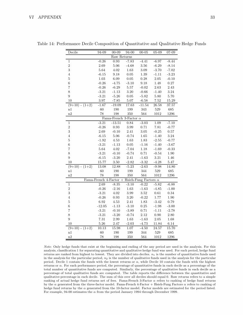
VI APPENDIX 33

Table 14: Performance Decile Composition of Quantitative and Qualitative Hedge Funds

Decile 94-09 00-09 94-00 00-05 05-09 07-09

Raw Returns

1 -0.26 0.93 -7.83 -4.41 -6.97 -8.442 2.69 5.06 -4.68 3.56 -6.29 -8.143 5.64 4.02 1.63 3.09 -3.70 -7.024 -6.15 9.18 0.05 1.39 -1.11 -3.235 1.03 6.09 0.05 0.28 2.05 -0.106 -0.26 -4.75 -3.10 9.18 1.48 0.277 -0.26 -6.29 5.57 -0.02 2.63 2.438 -3.21 -1.13 3.20 -0.66 -1.40 3.249 -3.21 -5.26 0.05 -5.82 5.80 5.7010 3.97 -7.85 5.07 -6.58 7.52 15.29

(9+10) - (1+2) -1.67 -19.09 17.63 -11.54 26.58 37.57n1 60 190 199 343 529 685n2 78 198 350 564 1012 1296

Fama-French 3-Factor α

1 -3.21 -13.51 0.84 -3.03 1.09 -7.102 -0.26 0.93 3.99 0.71 7.81 -0.773 2.69 -0.10 2.41 3.05 -0.25 0.574 -6.15 5.06 -0.74 1.65 -1.40 3.245 -1.92 4.53 1.63 1.83 -2.55 -0.776 -3.21 -1.13 0.05 -1.16 -1.40 -3.677 5.64 4.02 -7.04 1.18 -1.69 -0.338 -3.21 -0.10 -0.74 0.71 -0.54 1.909 -6.15 -3.20 2.41 -1.63 3.21 1.4610 15.77 3.50 -2.82 -3.32 -4.28 5.47

(9+10) - (1+2) 13.08 12.88 -5.23 -2.63 -9.98 14.80n1 60 190 199 344 529 685n2 78 198 350 564 1012 1296

Fama-French 4-Factor + Hsieh-Fung Factors α

1 2.69 -8.35 -3.10 -0.22 -5.82 -6.882 -0.26 -2.16 1.63 -1.63 -4.85 -1.003 -3.21 4.02 3.99 3.52 0.61 0.344 -0.26 0.93 3.20 -0.22 1.77 1.905 6.92 4.53 2.41 1.83 -3.42 0.796 -12.05 -1.13 -3.10 0.25 -1.98 -3.007 -3.21 -0.10 -3.89 0.71 -1.11 -2.788 -3.21 -3.20 -0.74 2.12 0.90 2.809 7.31 2.99 1.63 -1.63 2.05 1.6810 5.26 2.47 -2.03 -4.73 11.84 6.14

(9+10) - (1+2) 10.13 15.98 1.07 -4.50 24.57 15.70n1 60 190 199 344 529 685n2 78 198 350 564 1012 1296

Note: Only hedge funds that exist at the beginning and ending of the any period are used in the analysis. For thisanalysis, classification 1 for separating quantitative and qualitative hedge fund was used. For each period, hedge fundreturns are ranked from highest to lowest. They are divided into deciles. n1 is the number of quantitative funds usedin the analysis for the particular period, n2 is the number of qualitative funds used in the analysis for the particularperiod. Decile 1 contain the funds with the lowest returns or α, while Decile 10 contain the funds with the highestreturns or α. For each performance period, the percentage of quantitative funds in each decile as a percentage of thetotal number of quantitative funds are computed. Similarly, the percentage of qualitative funds in each decile as apercentage of total qualitative funds are computed. The table reports the difference between the quantitative andqualitative percentage in each decile. The sum of this over all deciles should equal 0. Raw returns refers to a simpleranking of actual hedge fund returns net of fees. Fama-French 3-Factor α refers to ranking of hedge fund returnsby the α generated from the three-factor model. Fama-French 4-Factor + Hsieh-Fung Factors α refers to ranking ofhedge fund returns by the α generated from the 10-factor model. Factor models are estimated for the period listed.For example, 94-00 estimates the α from the period January 1994 through December 1999.

VII FIGURES 34

VII Figures

05

00

00

10

00

00

15

00

00

20

00

00

AU

M (

in M

illio

ns o

f U

SD

)

1995 2000 2005 2010Year

Quantitative Qualitative

Figure 1: Growth of Quantitative and Qualitative Funds in AUM (Millions of Dollars). Note: Qual

funds normalized to value in database of Quant funds in January 1994 at $9.98B (Qual fund totalon this date was $18.61B)

REFERENCES 35

References

[1] Ackermann, C., McEnally, R. and D. Ravenscraft. “The Performance of Hedge Funds:

Risk, Return, and Incentives”. Journal of Finance, 54:833–874, June 1999.

[2] Agarwal, Vinik and Narayan Naik. “Risks and Portfolio Decisions Involving HedgeFunds”. The Review of Financial Studies, pages 63–98, Spring 2004.

[3] Ahmed, Parvez and Sudhir Nanda. “Performance of Enhanced Index and Quantitative

Equity Funds”. The Financial Review, 40:459–479, 2005.

[4] Breusch, T.S. “Testing for Autocorrelation in Dynamic Linear Models”. Australian Eco-

nomic Papers, 31:334–355, September 1978.

[5] Breusch, T.S. and A.R. Pagan. “A Simple Test for Heteroskedasticity and Random Co-

efficient Variation”. Econometrica, 47:1287–1294, 1979.

[6] Brown, S.J., Goetzmann, W.N., and R.G. Ibbotson. “Offshore Hedge Funds: Survivaland Performance 1989-1995”. Journal of Business, 72:91–117, January 1999.

[7] Brown, S.J., Goetzmann, W.N., Ibbotson, R.G., and S.A. Ross. “Survivorship Bias

in Performance Studies”. Review of Financial Studies, 5:553–580, Winter 1992.

[8] Chincarini, Ludwig B. and Daehwan Kim. Quantitative Equity Portfolio Management.McGraw-Hill, 2006.

[9] Fung, William and David A. Hsieh. “The Risk in Hedge Fund Strategies: Theory and

Evidence from Trend Followers”. The Review of Financial Studies, pages 313–341, Summer2001.

[10] Fung, William and David A. Hsieh. “Hedge Fund Benchmarks: A Risk Based Approach”.

Financial Analysts Journal, pages 65–80, September/October 2004.

[11] Godfrey, L.G. “Testing Against General Autoregressive and Moving Average Error Modelswhen the Regressors Include Lagged Dependent Variables”. Econometrica, 46:1293–1302, 1978.

[12] Goetzmann, William N., Ingersoll Jr., Jonathan and Zoran Ivkovic. “Monthly

Measurement of Daily Timers”. Journal of Financial and Quantitative Analysis, pages 257–291, September 2000.

[13] Henriksson, Roy D. and Robert C. Merton. “On Market Timing and Investment

Performance: II: Statistical Procedures for Evaluating Forecasting Skills”. Journal of Business,pages 513–533, 1981.

[14] Liang, Bing. “Hedge Funds: The Living and the Dead”. Journal of Financial and Quanti-

tative Analysis, 35:309–326, 2000.

[15] Merton, Robert C. “On Market Timing and Investment Performance. I. An EquilibriumTheory of Value for Market Forecasts”. Journal of Business, pages 363–406, July 1981.

[16] Newey, W. and K. West. “A Simple, Positive Semi-Definite, Heteroskedascity and Auto-

correlation Consistent Matrix”. Econometrica, pages 703–708, 1987.

[17] Stock, James H. and Mark W. Watson. Introduction to Econometrics. Pearson, AddisonWesley, 2007.

[18] Wooldridge, Jeffrey M. Introductory Econometrics: A Modern Approach. South-Western,

2009.

A Comparison of Quantitative and Qualitative Hedge … Comparison of Quantitative and Qualitative...

Documents

Transcript of A Comparison of Quantitative and Qualitative Hedge … Comparison of Quantitative and Qualitative...